Analysis of a finite element method for the Stokes–Poisson–Boltzmann equations

Abstract

We define a finite element method for the coupling of Stokes and nonlinear Poisson–Boltzmann equations. Using Banach contracting principle, the Babuška–Brezzi theory, and the Minty–Browder theorem, we show that the governing equations have a unique weak solution. We also show that the discrete problem is well-posed, establish Céa estimates, and derive convergence rates. We exemplify the properties of the proposed scheme via some numerical experiments showcasing convergence and applicability in the study of electro-osmotic flows in micro-channels.

2020 MSC codes: 65N30 (primary); 35J60, 76D07 (secondary).

Keywords: Stokes–Poisson–Boltzmann equations; Fixed-point analysis; Finite element discretisation; Error estimates.

1 Introduction

Scope.

Electrically charged flows are of utmost importance in chemistry applications that concern for example, the design of nanopores for biomedical devices and the modelling of water purification systems. One of the simplest processes to transport fluid without mechanical stimulation is electro-osmosis. The mobility of the fluid due to thin double layers that attract and repel ions in an electrolyte, can be described by the Stokes equations with a forcing term that depends on the charge of the electrolyte and an externally applied electric field. In a simplified scenario, the flow itself or its pressure gradients are not dominant enough to influence the distribution of the double layer electrostatic potential, and so the electric charge density can be simply related to the potential using (even simplified versions of) the Poisson–Boltzmann equation.

Regarding unique solvability and finite element (FE) discretisation for the Poisson–Boltzmann equation we refer to the work [6] (see also, e.g., [9, 10, 11]) that use, for example, a splitting between regular and singular contribution expansion and apply convex minimisation arguments, and show an $L^{\infty}$ bound for the solution using a cutoff-function approach. Here we take the regularised counterpart of this equation, which maintains the same type of nonlinearity (a hyperbolic sine) but does not include the distributional Dirac forcing terms. In addition, here we also include an advection term in the regularised potential equation, and following [9] we restrict the functional space of the double layer potential to a bounded set (in turn, permitting us to have a bounded nonlinear operator).

Outline.

The remainder of this section presents the strong form of the coupled system. Section 2 is devoted to the weak formulation and well-posedness using Banach fixed-point theory. In Section 3 we show the existence and uniqueness of discrete solution, and outline the a priori error analysis. Finally, in Section 4 we provide numerical examples of convergence and fully developed electro-osmotic flows in eccentric micro-tubes.

The Stokes–Poisson–Boltzmann equations.

Let us consider a Lipschitz bounded domain in $\mathbb{R}^{n}$, $n=2,3$ with boundary $\partial\Omega=\Gamma_{D}\cup\Gamma_{N}$ split into two parts where different types of boundary conditions will be considered, and denote by $\boldsymbol{n}$ the outward unit normal vector on the boundary. The domain is filled with an incompressible fluid subjected to pressure gradients and electric charges in an electrolyte. The set of equations that govern the stationary regime are written in term of fluid velocity $\boldsymbol{u}$, pressure $p$, and electrostatic double layer potential $\psi$, and read as follows

$$-\mu\boldsymbol{\Delta}\boldsymbol{u}+\nabla p =\boldsymbol{f}-\varepsilon\Delta\psi\mathbf{E} \text{in }\Omega,$$ (1.1a)

$$\operatorname{div}\boldsymbol{u} =0 \text{in }\Omega,$$ (1.1b)

$$\kappa(\psi)+\boldsymbol{u}\cdot\nabla\psi-\varepsilon\Delta\psi =g \text{in }\Omega,$$ (1.1c)

$$\boldsymbol{u}=\boldsymbol{0}\quad\text{and}\quad\psi =0 \text{on }\Gamma_{D},$$ (1.1d)

$$(\mu\boldsymbol{\nabla}\boldsymbol{u}-p\mathbf{I})\boldsymbol{n}=\boldsymbol{0}\quad\text{and}\quad\varepsilon\nabla\psi\cdot\boldsymbol{n} =0 \text{on }\Gamma_{N}.$$ (1.1e)

Here $\mathbf{I}$ is the identity tensor in $\mathbb{R}^{n\times n}$, $\mu$ is the fluid viscosity, $\boldsymbol{f}\in\mathbf{L}^{2}(\Omega)$ is a vector of external body forces, $\mathbf{E}\in\mathbf{L}^{\infty}(\Omega)$ is an externally applied electric field (typically along the longitudinal direction, and assumed uniformly bounded by $\bar{E}>0$), $\varepsilon$ is the electric permittivity of the electrolyte, $g\in L^{2}(\Omega)$ is an external source/sink of potential, and $\kappa(\psi)=k_{0}\sinh(k_{1}\psi)$ is the charge of the electrolyte as a nonlinear function of potential, where $k_{0}>0$ depends on the valence, the electron charge, and the bulk ion concentration, and $k_{1}>0$ depends additionally on the Boltzmann constant and the reference absolute temperature. Following [9, Lem. 2.1] we can assume that

• the potential is uniformly bounded between the values $\alpha\leq 0\leq\beta\in\mathbb{R}$.

In addition, we assume $\kappa(0)=0$, and that there exists $\bar{K},\underline{K}>0$ such that

• $|\kappa(s_{1})-\kappa(s_{2})|\leq\bar{K}|s_{1}-s_{2}|$ for all $s_{1},s_{2}\in[\alpha,\beta]$,

• $|\kappa(s_{1})-\kappa(s_{2})|\geq\underline{K}|s_{1}-s_{2}|$ for all $s_{1},s_{2}\in[\alpha,\beta]$.

Homogeneity of (1.1d)-(1.1e) is only assumed to simplify the exposition, however the results remain valid for more general assumptions.

2 Existence and uniqueness of weak solution

Weak formulation.

Consider the following test and trial functional spaces for velocity, double layer potential, and pressure, respectively

$$\mathbf{V}:=\{\boldsymbol{v}\in\mathbf{H}^{1}(\Omega):\boldsymbol{v}=\boldsymbol{0}\ \text{on}\ \Gamma_{D}\},\qquad\Phi_{0}:=\{\varphi\in H^{1}(\Omega):\varphi=0\ \text{on}\ \Gamma_{D}\},$$

$$\Phi:=\{\varphi\in H^{1}(\Omega):\varphi=0\ \text{on}\ \Gamma_{D}\ \text{and}\ \alpha\leq\varphi\leq\beta\},\qquad\mathrm{Q}:=L^{2}(\Omega).$$

Then, multiplying (1.1a)-(1.1c) by suitable test functions, integrating by parts, and employing the boundary conditions, we are left with the following weak formulation: find $(\boldsymbol{u},p,\psi)\in\mathbf{V}\times\mathrm{Q}\times\Phi$ such that

$$a(\boldsymbol{u},\boldsymbol{v})+A^{\psi}(\boldsymbol{u},\boldsymbol{v})+b(\boldsymbol{v},p) =F^{\psi}(\boldsymbol{v}) \forall\boldsymbol{v}\in\mathbf{V},$$ (2.1a)

$$b(\boldsymbol{u},q) =0 \forall q\in\mathrm{Q},$$ (2.1b)

$$(\kappa(\psi),\varphi)+c(\boldsymbol{u};\psi,\varphi)+d(\psi,\varphi) =G(\varphi) \forall\varphi\in\Phi_{0},$$ (2.1c)

where the following bilinear and trilinear forms are used

$$a(\boldsymbol{u},\boldsymbol{v}):=\mu\int_{\Omega}\boldsymbol{\nabla}\boldsymbol{u}:\boldsymbol{\nabla}\boldsymbol{v},\quad b(\boldsymbol{v},q):=-\int_{\Omega}\operatorname{div}\boldsymbol{v}\,q,$$

$$c(\boldsymbol{v};\psi,\varphi):=\int_{\Omega}(\boldsymbol{v}\cdot\nabla\psi)\varphi,\quad d(\psi,\varphi):=\varepsilon\int_{\Omega}\nabla\psi\cdot\nabla\varphi,$$

as well as (for a fixed $\hat{\psi}$) the following linear functionals and bilinear form

$$F^{\hat{\psi}}(\boldsymbol{v}):=\!\int_{\Omega}\{\boldsymbol{f}+[g-\kappa(\hat{\psi})]\mathbf{E}\}\cdot\boldsymbol{v},\ G(\varphi):=\!\int_{\Omega}g\,\varphi,\ A^{\hat{\psi}}(\boldsymbol{u},\boldsymbol{v}):=\!\int_{\Omega}[\boldsymbol{u}\cdot\nabla\hat{\psi}](\mathbf{E}\cdot\boldsymbol{v}).$$

The specific forms of $F^{\psi}(\bullet)$ and $A^{\psi}(\bullet,\bullet)$ are a consequence of rewriting the last source term in the right-hand side of (1.1a) using the potential equation (1.1c). The bilinear and trilinear forms above are uniformly bounded:

$$|a(\boldsymbol{u},\boldsymbol{v})|\leq\mu\,\|\boldsymbol{u}\|_{1,\Omega}\|\boldsymbol{v}\|_{1,\Omega},\quad|b(\boldsymbol{v},q)|\leq\|\boldsymbol{v}\|_{1,\Omega}\|q\|_{0,\Omega},$$

$$|d(\psi,\varphi)|\leq\varepsilon\|\psi\|_{1,\Omega}\|\varphi\|_{1,\Omega},\quad|{c}(\boldsymbol{v};\psi,\varphi)|\leq C_{\mathrm{Sob}}^{2}\|\boldsymbol{v}\|_{1,\Omega}\,\|\psi\|_{1,\Omega}\,\|\varphi\|_{1,\Omega},$$

$$|A^{\hat{\psi}}(\boldsymbol{u},\boldsymbol{v})|\leq C_{\mathrm{Sob}}^{2}\bar{E}\|\hat{\psi}\|_{1,\Omega}\|\boldsymbol{u}\|_{1,\Omega}\|\boldsymbol{v}\|_{1,\Omega},$$

where it suffices to apply Hölder’s inequality and the estimate $\|\phi\|_{L^{4}(\Omega)}\leq C_{\mathrm{Sob}}\|\phi\|_{1,\Omega}$, valid for all $\phi\in H^{1}(\Omega)$ (cf. [12, Th. 1.3.3]). So are the linear functionals in $\mathbf{V}^{\prime}$ (under the assumption that $\hat{\psi}$ is in a bounded set), and $\Phi^{\prime}$

$$|F^{\hat{\psi}}(\boldsymbol{v})|\leq\bigl{[}\|\boldsymbol{f}\|_{0,\Omega}+\bar{E}\|g\|_{0,\Omega}+\bar{K}\bar{E}\|\hat{\psi}\|_{1,\Omega}\bigr{]}\|\boldsymbol{v}\|_{1,\Omega},\quad|G(\varphi)|\leq\|g\|_{0,\Omega}\|\varphi\|_{1,\Omega}.$$

Using the Poincaré inequality $\|\phi\|_{1,\Omega}\leq C_{\mathrm{p}}|\phi|_{1,\Omega}$, with $C_{\mathrm{p}}>0$ and valid for all $\phi\in\{\varphi\in H^{1}(\Omega):\varphi=0\ \text{on}\ \Gamma_{D}\}$, it is not difficult to see that the bilinear forms $a(\bullet,\bullet)$ and $d(\bullet,\bullet)$ are coercive in $\mathbf{V}$ and $\Phi$, respectively,

$$|a(\boldsymbol{v},\boldsymbol{v})|\geq{\mu}[C_{\mathrm{p}}^{2}]^{-1}\|\boldsymbol{v}\|_{1,\Omega}^{2}\quad\forall\boldsymbol{v}\in\mathbf{V}\,,\quad|d(\varphi,\varphi)|\geq\varepsilon[{C_{\mathrm{p}}^{2}}]^{-1}\|\varphi\|_{1,\Omega}^{2}\quad\forall\varphi\in\Phi_{0}.$$

Furthermore, $b(\bullet,\bullet)$ satisfies the following inf-sup condition (see, e.g., [8])

$$\sup_{\boldsymbol{v}\in\mathbf{V}\setminus\{\boldsymbol{0}\}}\frac{b(\boldsymbol{v},q)}{\|\boldsymbol{v}\|_{1,\Omega}}\geq\beta\,\|q\|_{0,\Omega}\quad\forall q\in\mathrm{Q}.$$

Well-posedness analysis.

We will employ a fixed-point argument in combination with the Babuška–Brezzi theory [4] and the Minty–Browder theorem [7]. The analysis closely follows the approach in, e.g., [2, 5] for Boussinesq-type of problems where one separates the incompressible flow equations from the nonlinear transport equation and then connects them back using Banach’s fixed-point theorem. First, consider the following set

$$\mathrm{Z}:=\bigl{\{}\hat{\psi}\in\Phi:\quad\|\hat{\psi}\|_{1,\Omega}\leq{\mu}[{2C_{\mathrm{p}}^{2}C_{\mathrm{Sob}}^{2}\bar{E}}]^{-1}\bigr{\}},$$ (2.2)

and, for a fixed $\hat{\psi}\in\mathrm{Z}$, the problem of finding $(\boldsymbol{u},p)\in\mathbf{V}\times\mathrm{Q}$ such that

$$\begin{array}[]{clc}a(\boldsymbol{u},\boldsymbol{v})+A^{\hat{\psi}}(\boldsymbol{u},\boldsymbol{v})+b(\boldsymbol{v},p)&=F^{\hat{\psi}}(\boldsymbol{v})&\forall\boldsymbol{v}\in\mathbf{V},\\ b(\boldsymbol{u},q)&=0&\forall q\in\mathrm{Q}.\end{array}$$ (2.3)

Owing to the unique solvability of the Stokes equations with mixed boundary conditions [8] (in turn derived from the following properties of $[a+A^{\hat{\psi}}](\bullet,\bullet)$

$$|a(\boldsymbol{u},\boldsymbol{v})+A^{\hat{\psi}}(\boldsymbol{u},\boldsymbol{v})| \leq\bigl{(}\mu+{\mu}[{2C_{\mathrm{p}}^{2}}]^{-1}\bigr{)}\,\|\boldsymbol{u}\|_{1,\Omega}\|\boldsymbol{v}\|_{1,\Omega},$$

$$|a(\boldsymbol{v},\boldsymbol{v})+A^{\hat{\psi}}(\boldsymbol{v},\boldsymbol{v})| \geq{\mu}[{2C_{\mathrm{p}}^{2}}]^{-1}\,\|\boldsymbol{v}\|_{1,\Omega}^{2},$$ (2.4)

which arise from the properties of $a(\bullet,\bullet)$ and $A^{\hat{\psi}}(\bullet,\bullet)$, the definition of $\mathrm{Z}$, and the continuity and stability of $b(\bullet,\bullet)$), we conclude that the operator

$$\mathcal{S}^{\mathrm{flow}}:\Phi\to\mathbf{V}\times\mathrm{Q},\quad\hat{\psi}\mapsto\mathcal{S}^{\mathrm{flow}}(\hat{\psi})=(\mathcal{S}^{\mathrm{flow}}_{1}(\hat{\psi}),\mathcal{S}^{\mathrm{flow}}_{2}(\hat{\psi})):=(\boldsymbol{u},p),$$

is well-defined. Moreover, the continuous dependence on data provided by the Babuška–Brezzi theory gives, in particular, that

$$\|\boldsymbol{u}\|_{1,\Omega}\leq 2C_{\mathrm{p}}^{2}\mu^{-1}\bigl{(}\|\boldsymbol{f}\|_{0,\Omega}+\bar{E}\|g\|_{0,\Omega}+\bar{K}\bar{E}\|\hat{\psi}\|_{1,\Omega}\bigr{)}.$$ (2.5)

On the other hand, associated with the velocity, we define the following set

$$\mathbf{W}:=\bigl{\{}\hat{\boldsymbol{u}}\in\mathbf{V}:\quad\|\hat{\boldsymbol{u}}\|_{1,\Omega}\leq{\varepsilon}[{2C_{\mathrm{p}}^{2}C_{\mathrm{Sob}}^{2}}]^{-1}\bigr{\}},$$ (2.6)

and consider, for a fixed $\hat{\boldsymbol{u}}\in\mathbf{W}$, the problem of finding $\psi\in\Phi$ such that

$$(\kappa(\psi),\varphi)+c(\hat{\boldsymbol{u}};\psi,\varphi)+d(\psi,\varphi)=G(\varphi)\qquad\forall\varphi\in\Phi_{0}.$$ (2.7)

Using Hölder and Cauchy–Schwarz inequalities we proceed to verify that the operator associated with this problem is bounded

$$|(\kappa(\psi),\varphi)+c(\hat{\boldsymbol{u}};\psi,\varphi)+d(\psi,\varphi)|\leq(\bar{K}+\varepsilon+C_{\mathrm{Sob}}^{2}\|\hat{\boldsymbol{u}}\|_{1,\Omega})\,\|\psi\|_{1,\Omega}\|\varphi\|_{1,\Omega}.$$

Next we can use the coercivity of $d(\bullet,\bullet)$, the definition of $\mathbf{W}$, and the monotonicity of $\kappa(\bullet)$, to obtain the strong monotonicity of the solution operator

$$(\kappa(\psi_{1})-\kappa(\psi_{2}),\psi_{1}-\psi_{2})+c(\hat{\boldsymbol{u}};\psi_{1}-\psi_{2},\psi_{1}-\psi_{2})+d(\psi_{1}-\psi_{2},\psi_{1}-\psi_{2})$$

$$\qquad\geq{\varepsilon}[{2C_{\mathrm{p}}^{2}}]^{-1}\|\psi_{1}-\psi_{2}\|^{2}_{1,\Omega}\qquad\forall\,\psi_{1},\psi_{2}\in\Phi.$$ (2.8)

Then the Minty–Browder theorem gives that $\exists!\,\psi\in\Phi$ so the map

$$\mathcal{S}^{\mathrm{elec}}:\mathbf{V}\to\Phi,\quad\hat{\boldsymbol{u}}\mapsto\mathcal{S}^{\mathrm{elec}}(\hat{\boldsymbol{u}})=\psi,$$

is well-defined. In addition, using (2), we have that the solution satisfies

$$\|\psi\|_{1,\Omega}\leq{2C_{\mathrm{p}}^{2}}{\varepsilon}^{-1}\|g\|_{0,\Omega}.$$ (2.9)

Then we introduce an operator equivalent to the solution map of (2.1):

$$\mathbf{T}:\mathbf{W}\to\mathbf{W},\qquad\psi\mapsto\mathbf{T}(\psi):=\mathcal{S}^{\mathrm{flow}}_{1}(\mathcal{S}^{\mathrm{elec}}(\hat{\boldsymbol{u}})).$$ (2.10)

Lemma 2.1.

Assume that $\boldsymbol{f}\in\mathbf{L}^{2}(\Omega)$ and $g\in L^{2}(\Omega)$ satisfies

$$4C_{\mathrm{p}}^{4}C_{\mathrm{Sob}}^{2}[\mu\varepsilon]^{-1}\bigl{(}1+\bar{E}+2\bar{K}\bar{E}C_{\mathrm{p}}^{2}{\varepsilon}^{-1}\bigr{)}(\|\boldsymbol{f}\|_{0,\Omega}+\|g\|_{0,\Omega})\leq 1.$$ (2.11)

Then, the operator $\mathbf{T}$ is well-defined and $\mathbf{T}(\mathbf{W})\subseteq\mathbf{W}$.

Proof.

Given $\hat{\boldsymbol{u}}\in\mathbf{W}$, (2.11) implies $\frac{4C_{\mathrm{p}}^{4}C_{\mathrm{Sob}}^{2}\bar{E}}{\mu\varepsilon}\|g\|_{0,\Omega}\leq 1$. Combining this with (2.9) gives $\mathcal{S}^{\mathrm{elec}}(\hat{\boldsymbol{u}})\in\mathrm{Z}$. Using that $\mathcal{S}^{\mathrm{elec}}$ and $\mathcal{S}^{\mathrm{flow}}$ are well-defined, it follows that $\mathbf{T}$ is well-defined. Moreover, from (2.5) and (2.9), we obtain

$$\|\mathcal{S}^{\mathrm{flow}}_{1}(\mathcal{S}^{\mathrm{elec}}(\hat{\boldsymbol{u}}))\|_{1,\Omega} \leq 2C_{\mathrm{p}}^{2}\mu^{-1}\bigl{(}\|\boldsymbol{f}\|_{0,\Omega}+\bar{E}\|g\|_{0,\Omega}+\bar{K}\bar{E}{2C_{\mathrm{p}}^{2}}{\varepsilon}^{-1}\|g\|_{0,\Omega}\bigr{)}.$$

Combining this with the small data assumption (2.11) and the second equation in (2.3), we conclude that $\mathbf{T}(\hat{\boldsymbol{u}})\in\mathbf{W}$, thereby completing the proof. ∎

Theorem 1.

Assume that (2.11) holds, and assume that

$$4C_{\mathrm{p}}^{4}C_{\mathrm{Sob}}^{2}\bar{E}[\mu\varepsilon^{2}]^{-1}\,(\varepsilon+2C_{\mathrm{p}}^{2}\bar{K})\,\|g\|_{0,\Omega}<1.$$ (2.12)

Then, $\mathbf{T}$ has a unique fixed-point $\boldsymbol{u}\in\mathbf{W}$. Equivalently, problem (2.1) has a unique solution $(\boldsymbol{u},p,\psi)\in\mathbf{V}\times\mathrm{Q}\times\Phi$ with $\boldsymbol{u}\in\mathbf{W}$. Moreover,

$$\|\psi\|_{1,\Omega}\lesssim\|g\|_{0,\Omega}{\quad\hbox{and}\quad}\|\boldsymbol{u}\|_{1,\Omega}+\|p\|_{0,\Omega}\lesssim\|\boldsymbol{f}\|_{0,\Omega}+\|g\|_{0,\Omega}.$$ (2.13)

Proof.

Given $\hat{\boldsymbol{u}}_{1},\hat{\boldsymbol{u}}_{2}\in\mathbf{W}$, we let $\psi_{1},\psi_{2}\in\Phi_{0}$ such that $\mathcal{S}^{\mathrm{elec}}(\hat{\boldsymbol{u}}_{1})=\psi_{1}$ and $\mathcal{S}^{\mathrm{elec}}(\hat{\boldsymbol{u}}_{2})=\psi_{2}$. Using (2.7), adding $\pm c(\hat{\boldsymbol{u}}_{1},\psi_{2},\varphi)$, taking $\varphi=\psi_{1}-\psi_{2}$, and applying (2) along with the boundedness of $c(\bullet;\bullet,\bullet)$, we obtain

$$\|\mathcal{S}^{\mathrm{elec}}(\hat{\boldsymbol{u}}_{1})-\mathcal{S}^{\mathrm{elec}}(\hat{\boldsymbol{u}}_{2})\|_{1,\Omega}\leq 2C_{\mathrm{Sob}}^{2}C_{\mathrm{p}}^{2}\varepsilon^{-1}\|\psi_{2}\|_{1,\Omega}\|\hat{\boldsymbol{u}}_{1}-\hat{\boldsymbol{u}}_{2}\|_{1,\Omega}.$$ (2.14)

Similarly, let $\hat{\psi}_{1},\hat{\psi}_{2}\in\Phi$ and $(\boldsymbol{u}_{1},p_{1}),(\boldsymbol{u}_{2},p_{2})\in\mathbf{V}\times\mathrm{Q}$, such that $\mathcal{S}^{\mathrm{flow}}(\hat{\psi}_{1})=(\boldsymbol{u}_{1},p_{1})$ and $\mathcal{S}^{\mathrm{flow}}(\hat{\psi}_{2})=(\boldsymbol{u}_{2},p_{2})$. Using (2.3), adding $\pm A^{\hat{\psi}_{1}}(\boldsymbol{u}_{2},\boldsymbol{v})$, taking $\varphi=\psi_{1}-\psi_{2}$, and applying the coercivity of $a+A^{\hat{\psi}}(\bullet,\bullet)$ (c.f. (2)), along with the continuity of $A^{\hat{\psi}}(\bullet,\bullet)$ and the assumptions for $\kappa(\bullet)$, we have

$$\|\mathcal{S}^{\mathrm{flow}}_{1}(\hat{\psi}_{1})-\mathcal{S}^{\mathrm{flow}}_{1}(\hat{\psi}_{2})\|_{1,\Omega}\leq 2C_{\mathrm{p}}^{2}\bar{E}\mu^{-1}(C_{\mathrm{Sob}}^{2}\|\boldsymbol{u}_{2}\|_{1,\Omega}+\bar{K})\|\hat{\psi}_{1}-\hat{\psi}_{2}\|_{1,\Omega}.$$ (2.15)

Thus, combining (2.14) with (2.15), we have

$$\|\mathbf{T}(\hat{\boldsymbol{u}}_{1})-\mathbf{T}(\hat{\boldsymbol{u}}_{2})\|_{1,\Omega}\leq\|\mathcal{S}^{\mathrm{flow}}_{1}(\mathcal{S}^{\mathrm{elec}}(\hat{\boldsymbol{u}}_{1}))-\mathcal{S}^{\mathrm{flow}}_{1}(\mathcal{S}^{\mathrm{elec}}(\hat{\boldsymbol{u}}_{2}))\|_{1,\Omega}$$

$$\quad\leq 2C_{\mathrm{p}}^{2}\bar{E}\mu^{-1}(C_{\mathrm{Sob}}^{2}\|\boldsymbol{u}_{2}\|_{1,\Omega}+\bar{K})2C_{\mathrm{Sob}}^{2}C_{\mathrm{p}}^{2}\varepsilon^{-1}\|\mathcal{S}^{\mathrm{elec}}(\hat{\boldsymbol{u}}_{2})\|_{1,\Omega}\|\hat{\boldsymbol{u}}_{1}-\hat{\boldsymbol{u}}_{2}\|_{1,\Omega},$$

then, using the fact that $\mathcal{S}^{\mathrm{elec}}(\hat{\boldsymbol{u}}_{2})$ satisfies (2.9) and $\hat{\boldsymbol{u}}_{2}\in\mathbf{W}$, we obtain

$$\|\mathbf{T}(\hat{\boldsymbol{u}}_{1})-\mathbf{T}(\hat{\boldsymbol{u}}_{2})\|_{1,\Omega}\leq{8C_{\mathrm{p}}^{6}C_{\mathrm{Sob}}^{2}\bar{E}}[{\mu\varepsilon^{2}}]^{-1}\bigl{(}{\varepsilon}[{2C_{\mathrm{p}}^{2}}]^{-1}+\bar{K}\bigr{)}\,\|g\|_{0,\Omega}\|\hat{\boldsymbol{u}}_{1}-\hat{\boldsymbol{u}}_{2}\|_{1,\Omega},$$

which together with (2.12) and the Banach fixed-point theorem implies that $\mathbf{T}$ has a unique fixed point in $\mathbf{W}$. Finally, the first estimate in (2.13) is derived similarly to (2.9), while the second follows directly from [8, Th. 2.34]. ∎

3 Finite element discretisation

Let us denote $\mathcal{T}_{h}$ a shape-regular simplicial mesh of $\Omega$ with mesh-size $h:=\max\{h_{K}:K\in\mathcal{T}_{h}\}$. Given $k\geq 1$, the generalised Taylor–Hood FE spaces for the approximation of velocity, pressure, and potential, are

$$\mathbf{V}_{h} :=\{\boldsymbol{v}_{h}\in\mathbf{C}^{0}(\Omega):\boldsymbol{v}_{h}|_{K}\in[\mathbb{P}_{k+1}(K)]^{n},\ \forall K\in\mathcal{T}_{h},\ \boldsymbol{v}_{h}=\boldsymbol{0}\ \text{on}\ \Gamma_{D}\},$$

$$\mathrm{Q}_{h} :=\{q_{h}\in C^{0}(\Omega):q_{h}|_{K}\in\mathbb{P}_{k}(K),\,K\in\mathcal{T}_{h}\},$$

$$\Phi_{h} :=\{\varphi_{h}\in C^{0}(\Omega):\varphi_{h}|_{K}\in\mathbb{P}_{k+1}(K),\ \forall K\in\mathcal{T}_{h},\ \varphi_{h}=0\ \text{on}\ \Gamma_{D}\}.$$

The FE scheme then reads: find $(\boldsymbol{u}_{h},p_{h},\psi_{h})\in\mathbf{V}_{h}\times\mathrm{Q}_{h}\times\Phi_{h}$ such that

$$a(\boldsymbol{u}_{h},\boldsymbol{v}_{h})+A^{\psi_{h}}(\boldsymbol{u}_{h},\boldsymbol{v}_{h})+b(\boldsymbol{v}_{h},p_{h}) =F^{\psi_{h}}(\boldsymbol{v}_{h}) \forall\boldsymbol{v}_{h}\in\mathbf{V}_{h},$$ (3.1a)

$$b(\boldsymbol{u}_{h},q_{h}) =0 \forall q_{h}\in\mathrm{Q}_{h},$$ (3.1b)

$$(\kappa(\psi_{h}),\varphi_{h})+c(\boldsymbol{u}_{h};\psi_{h},\varphi_{h})+d(\psi_{h},\varphi_{h}) =G(\varphi_{h}) \forall\varphi_{h}\in\Phi_{h}.$$ (3.1c)

The unique solvability of the discrete problem can be shown using similar techniques as for the continuous counterpart.

Theorem 2.

Assume that the hiphotesis of Theorem 1 hold. Then, (3.1) has a unique solution $(\boldsymbol{u}_{h},p_{h},\psi_{h})\in\mathbf{V}_{h}\times\mathrm{Q}_{h}\times\Phi_{h}$. Moreover,

$$\|\psi\|_{1,\Omega}\lesssim\|g\|_{0,\Omega}{\quad\hbox{and}\quad}\|\boldsymbol{u}\|_{1,\Omega}+\|p\|_{0,\Omega}\lesssim\|\boldsymbol{f}\|_{0,\Omega}+\|g\|_{0,\Omega}.$$ (3.2)

Theorem 3.

Let $(\boldsymbol{u},p,\psi),(\boldsymbol{u}_{h},p_{h},\psi_{h})$ be the continuous and discrete solutions. Then, assuming that the data satisfies

$$\bigl{(}1+4\varepsilon^{-1}\bar{K}\bar{E}C_{\mathrm{p}}^{2}\bigr{)}4\varepsilon^{-1}C_{\mathrm{Sob}}^{2}C_{\mathrm{p}}^{2}\|g\|_{0,\Omega}\leq 1,$$ (3.3)

we have the following bound, with hidden constant independent of $h$,

$$\|\boldsymbol{u}-\boldsymbol{u}_{h}\|_{1,\Omega}+\|p-p_{h}\|_{0,\Omega}+\|\psi-\psi_{h}\|_{1,\Omega}\lesssim\mathrm{dist}(\boldsymbol{u},\mathbf{V}_{h})+\mathrm{dist}(p,\mathrm{Q}_{h})+\mathrm{dist}(\psi,\Phi_{h}).$$

Proof.

For a given $(\hat{\boldsymbol{v}}_{h},\hat{q}_{h},\hat{\varphi}_{h})\in\mathbf{V}_{h}\times Q_{h}\times\Phi_{h}$, let us decompose errors using $\mbox{\boldmath{$\xi$}}_{\boldsymbol{u}}:=\boldsymbol{u}-\hat{\boldsymbol{v}}_{h}$, $\mbox{\boldmath{$\chi$}}_{\boldsymbol{u}}:=\hat{\boldsymbol{v}}_{h}-\boldsymbol{u}_{h}$, $\xi_{p}:=p-\hat{q}_{h}$, $\chi_{p}:=\hat{q}_{h}-p_{h}$, $\xi_{\psi}:=\psi-\hat{\varphi}_{h}$ and $\chi_{\psi}:=\hat{\varphi}_{h}-\psi_{h}$. Proceeding as in Theorem 1, we can obtain

$$\|\mbox{\boldmath{$\chi$}}_{\boldsymbol{u}}\|+\|\chi_{p}\|+\|\chi_{\psi}\| \leq\frac{4}{\varepsilon}\bar{K}\bar{E}C_{\mathrm{Sob}}^{2}C_{\mathrm{p}}^{2}\|\psi_{h}\|_{1,\Omega}\|\boldsymbol{u}-\boldsymbol{u}_{h}\|_{1,\Omega}+\varepsilon\|\xi_{\psi}\|_{1,\Omega}$$

$$\ +C_{\mathrm{Sob}}^{2}\|\psi\|_{1,\Omega}\|\boldsymbol{u}-\boldsymbol{u}_{h}\|_{1,\Omega}+(1+\mu)\|\mbox{\boldmath{$\xi$}}_{\boldsymbol{u}}\|_{1,\Omega}+\|\xi_{p}\|_{0,\Omega}$$

$$\ +C_{\mathrm{Sob}}^{2}\|\boldsymbol{u}_{h}\|_{1,\Omega}\|\xi_{\psi}\|_{1,\Omega}+C_{\mathrm{Sob}}^{2}\bar{E}\|\psi_{h}\|_{1,\Omega}\|\xi_{\boldsymbol{u}}\|_{1,\Omega}.$$

Then, from (2.13) and (3.2), assumption (3.3), and the fact that $(\hat{\boldsymbol{v}}_{h},\hat{q}_{h},\hat{\varphi}_{h})\in\mathbf{V}_{h}\times Q_{h}\times\Phi_{h}$ is arbitrary, the desired result is obtained. ∎

And the following result is a direct consequence of Theorem 3 and standard interpolation properties for Taylor–Hood FEs [8].

Theorem 4.

Let $(\boldsymbol{u},p,\psi),(\boldsymbol{u}_{h},p_{h},\psi_{h})$ be the continuous and discrete solutions assuming $\boldsymbol{u}\in\mathbf{V}\cap\mathbf{H}^{s+1}(\Omega)$, $p\in H^{s}(\Omega)$, and $\psi\in\Phi\cap H^{s+1}(\Omega)$, for some $s\in(1/2,k+1]$. Then, there exists $C>0$, independent of $h$, such that

$$\|\boldsymbol{u}-\boldsymbol{u}_{h}\|_{1,\Omega}+\|p-p_{h}\|_{0,\Omega}+\|\psi-\psi_{h}\|_{1,\Omega}\leq C\,h^{s}\{\|\boldsymbol{u}\|_{1+s,\Omega}+|p|_{s,\Omega}+\|\psi\|_{1+s,\Omega}\}.$$

4 Numerical results

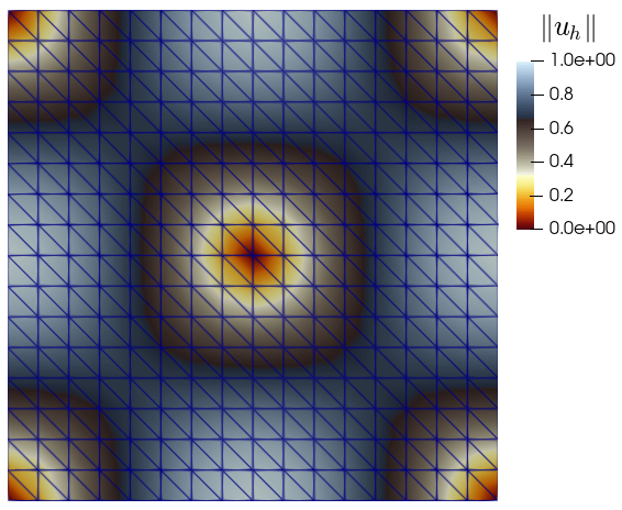
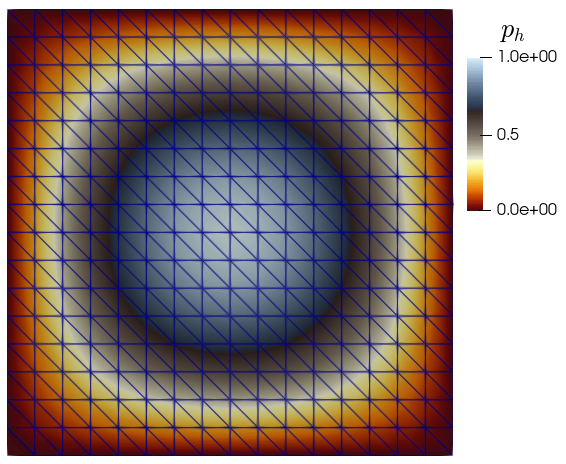
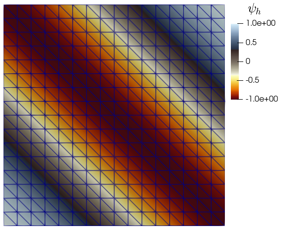
Figure 4.1: Approximate solutions for the convergence test on the unit square domain, using the lowest-order Taylor–Hood elements.

We now provide two simple computational tests confirming the convergence of the method and simulating electrically charged fluid in a container. They have been carried out with the library Gridap [3]. We use a Newton–Raphson method with a residual tolerance of $10^{-7}$. In the first test, the convergence rates from Theorem 4 are studied using the unit square domain $\Omega=(0,1)^{2}$ and the following manufactured solutions to (1.1)

$$\boldsymbol{u}:=\begin{pmatrix}\cos(\pi x)\sin(\pi y)\\ -\sin(\pi x)\cos(\pi y)\end{pmatrix},\quad p:=\sin(\pi x)\sin(\pi y),\quad\psi:=\cos(\pi(x+y))$$

The Dirichlet boundary corresponds to the bottom and right segments and the Neumann boundary is the remainder. The constants assume unity values $k_{0}=k_{1}=\mu=\varepsilon=1$, $\mathbf{E}=(0,-1)^{\tt t}$, and the forcing term and non-homogeneous boundary data are computed from the manufactured solutions. The error decay is reported in Table 4.1, where we also tabulate rates of convergence $\texttt{r}(\cdot)=\log(\texttt{e}_{(\cdot)}/\tilde{\texttt{e}}_{(\cdot)})[\log(h/\tilde{h})]^{-1}$, where $\texttt{e},\tilde{\texttt{e}}$ denote errors generated on two consecutive meshes of sizes $h$ and $\tilde{h}$, respectively. Optimal convergence is verified in all fields, and the approximate solutions plotted in Figure 4.1 show well-resolved profiles even for coarse meshes.

DoF	$h$	$\texttt{e}(\boldsymbol{u})$	$\texttt{r}(\boldsymbol{u})$	$\texttt{e}(p)$	$\texttt{r}(p)$	$\texttt{e}(\psi)$	$\texttt{r}(\psi)$	it
$k=1$
57	0.7071	6.50e-01	$\star$	2.21e-01	$\star$	2.65e-01	$\star$	4
217	0.3536	1.79e-01	1.860	3.49e-02	2.658	6.96e-02	1.927	4
849	0.1768	4.66e-02	1.943	6.97e-03	2.325	1.78e-02	1.969	4
3361	0.0884	1.18e-02	1.979	1.64e-03	2.089	4.48e-03	1.987	4
13377	0.0442	2.97e-03	1.992	4.04e-04	2.022	1.12e-03	1.995	4
53377	0.0221	7.45e-04	1.997	1.01e-04	2.006	2.82e-04	1.998	4
213249	0.0110	1.86e-04	1.998	2.51e-05	2.001	7.05e-05	1.999	4
$k=2$
133	0.7071	1.38e-01	$\star$	3.01e-02	$\star$	3.39e-02	$\star$	4
513	0.3536	1.86e-02	2.899	4.12e-03	2.871	4.37e-03	2.955	4
2017	0.1768	2.35e-03	2.980	5.41e-04	2.926	5.51e-04	2.988	4
8001	0.0884	2.95e-04	2.995	6.87e-05	2.979	6.92e-05	2.995	4
31873	0.0442	3.69e-05	2.999	8.62e-06	2.995	8.66e-06	2.998	4
127233	0.0221	4.61e-06	2.999	1.08e-06	2.997	1.09e-06	2.994	4
508417	0.0110	5.80e-07	2.992	1.51e-07	2.939	1.63e-07	2.939	4

Table 4.1: Convergence history. Errors, experimental rates, and Newton iteration count for FE families using polynomial degrees $k=1,2$.

Next we study the electro-osmotic and pressure-driven mixing of a fluid in a micro-annulus following the configuration of [1], but instead of bipolar coordinates we employ a full 3D Cartesian system. The model parameters are set to $\mu=10^{-2}$, $r_{1}=1$, $r_{2}=2$, $H=0.75$, and $k_{0}=\frac{(H-r_{1}-r_{2})(H-r_{1}+r_{2})(H+r_{1}-r_{2})(H+r_{1}+r_{2})}{2H}$, $k_{1}=1$, $\mathbf{E}=(0,0,1)^{\tt t}$. On the outer annulus we impose $\psi=2$, on the inner one we set $\psi=1$ and leave zero-flux boundary conditions elsewhere. We set $\boldsymbol{u}=(0,0,1)^{\tt t}$ on the bottom face, no slip velocity on the inner and outer annulus $\boldsymbol{u}=\boldsymbol{0}$, and outflow conditions on the top face. For this test we discard advection (so that only the charge and inlet velocity determine the flow patterns). The results in Figure 4.2 show a higher electro-osmotic fluid mobility near the narrow part of the channel, and a distribution of the double layer potential comparable to the profiles obtained in [1].

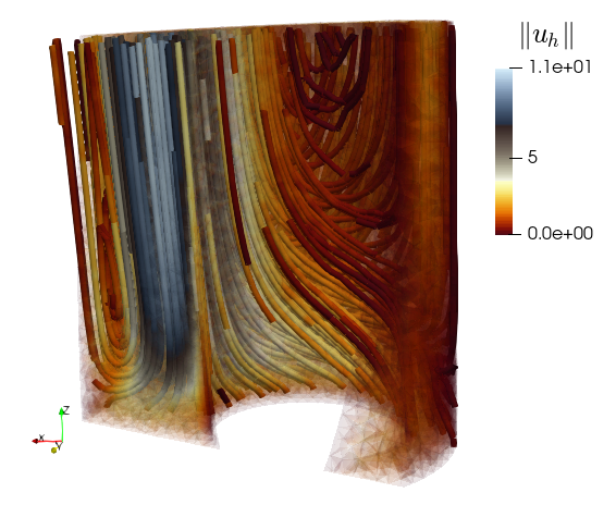
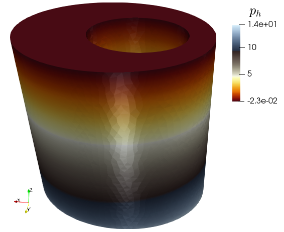
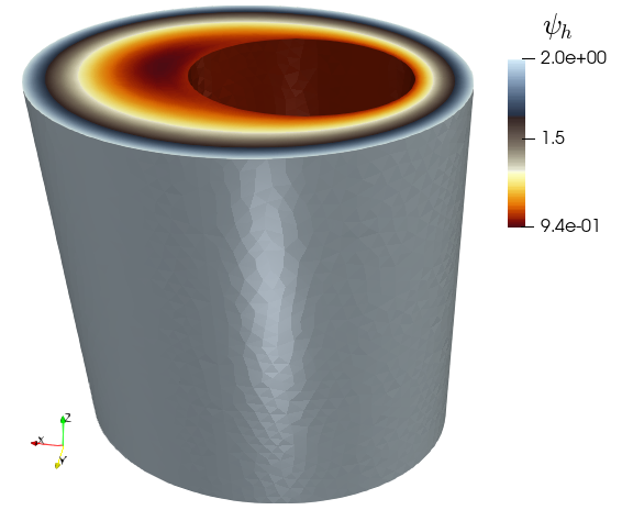
Figure 4.2: Approximate velocity magnitude and streamlines, pressure profile, and potential for the flow-potential test using Taylor–Hood elements.

Acknowledgements.

This research has been supported by the Australian Research Council through the Future Fellowship FT220100496 and Discovery Project DP22010316; and by the National Research and Development Agency (ANID) of Chile through the postdoctoral grant Becas Chile 74220026.

References

• Akyildiz et al. [2019] F. T. Akyildiz, A. F. AlSohaim, and N. Kaplan. Electro-osmotic and pressure-driven flow in an eccentric microannulus. Zeitschr. Nat. A, 74(6):513–521, 2019.
• Alvarez et al. [2021] M. Alvarez, G. N. Gatica, and R. Ruiz-Baier. A mixed-primal finite element method for the coupling of Brinkman–Darcy flow and nonlinear transport. IMA J. Numer. Anal., 41(1):381–411, 2021.
• Badia et al. [2022] S. Badia, A. F. Martín, and F. Verdugo. GridapDistributed: a massively parallel finite element toolbox in Julia. J. Open Source Softw., 7(74):4157, 2022.
• Boffi et al. [2013] D. Boffi, F. Brezzi, and M. Fortin. Mixed Finite Element Methods and Applications, volume 44. Springer-Verlag, Berlin, 2013.
• Caucao et al. [2020] S. Caucao, R. Oyarzúa, and S. Villa-Fuentes. A new mixed-FEM for steady-state natural convection models allowing conservation of momentum and thermal energy. Calcolo, 57(4):36, 2020.
• Chen et al. [2007] L. Chen, M. Holst, and J. Xu. The finite element approximation of the nonlinear Poisson-Boltzmann equation. SIAM J. Numer. Anal., 45(6):2298–2320, 2007.
• Ciarlet [2013] P. G. Ciarlet. Linear and Nonlinear Functional Analysis with Applications. SIAM, Society for Industrial and Applied Mathematics, 2013.
• Ern and Guermond [2004] A. Ern and J.-L. Guermond. Theory and Practice of Finite Elements. Applied Mathematical Sciences, 159. Springer-Verlag, New York, 2004.
• Holst et al. [2012] M. Holst, J. McCammon, Z. Yu, Y. Zhou, and Y. Zhu. Adaptive finite element modeling techniques for the Poisson-Boltzmann equation. Comm. Comput. Phys., 11(1):179–214, Jan. 2012.
• Iglesias and Nakov [2022] J. A. Iglesias and S. Nakov. Weak formulations of the nonlinear Poisson-Boltzmann equation in biomolecular electrostatics. J. Math. Anal. Appl., 511(1):126065, 2022.
• Kraus et al. [2020] J. Kraus, S. Nakov, and S. I. Repin. Reliable numerical solution of a class of nonlinear elliptic problems generated by the Poisson–Boltzmann equation. Comput. Methods Appl. Math., 20(2):293–319, 2020.
• Quarteroni and Valli [1994] A. Quarteroni and A. Valli. Numerical Approximation of Partial Differential Equations, volume 23 of Springer Series in Computational Mathematics. Springer-Verlag, Berlin, 1994.