Looking To The Horizon: Probing Evolution in the Black Hole Spectrum With GW Catalogs

Abstract

The population of black holes observed via gravitational waves currently covers the local universe up to a redshift $z\lesssim 1$, for the most massive merging binaries, or $z\lesssim 0.25$ for low-mass BH binaries (BBH). Evolution of the BBH mass spectrum over cosmic time will be a significant probe of formation channels and environments. We demonstrate a reconstruction of the BBH merger rate, allowing for general dependence on binary masses and luminosity distance or redshift and accounting for selection effects, via iterative kernel density estimation (KDE) with optimized multidimensional bandwidths. Performing such reconstructions under a range of detailed assumptions, we see no significant evidence for the evolution of BBH masses with redshift, over the range where detected events are available; at most, a possible trend towards increasing merger rate with redshift for primary masses $m_{1}\gtrsim 50\,M_{\odot}$ is supported. We compare these findings with previous investigations and caution against over-interpreting the current, sparse, data. Significantly upgraded detectors and/or facilities, and longer observing times, are required to harness any correlations of the BBH mass distribution with redshift.

I Introduction

The detection of gravitational waves (GWs) Abbott et al. (2016, 2019a, 2021a, 2024, 2023a) from merging binary black holes (BBHs) by advanced LIGO and Virgo and KAGRA Aasi et al. (2015); Acernese et al. (2015); Akutsu et al. (2021) has opened a new avenue for studying the astrophysical population of black holes Abbott et al. (2019b, 2021b, 2023b). The analysis of BBH populations using GW observations provides critical insights into their formation channels, mass distribution, spin properties, and their evolution across cosmic time. Gravitational wave observations have revealed that merger rates likely increase with redshift, aligning with the history of cosmic star formation Madau and Dickinson (2014); Fishbach et al. (2018); Callister et al. (2020); Abbott et al. (2023b); Schiebelbein-Zwack and Fishbach (2024). Evidence has also emerged for characteristic features in the (primary) mass distribution, such as peaks near $10\,M_{\odot}$, and $35\,M_{\odot}$ Tiwari and Fairhurst (2021); Sadiq et al. (2022); Farah et al. (2023), and that the majority of binaries display nearly equal mass ratios Talbot and Thrane (2018); Tiwari (2022); Farah et al. (2024); Sadiq et al. (2024a). Potential astrophysical correlations between source parameters have been analyzed to investigate binary formation channels; here we will focus on both the mass spectrum and evolution over cosmic time or equivalently over redshift Fishbach et al. (2018); Mapelli et al. (2019); Abbott et al. (2023b); van Son et al. (2022); Callister and Farr (2024); Edelman et al. (2023); Karathanasis et al. (2023); Rinaldi et al. (2024); Heinzel et al. (2024a); Lalleman et al. (2025).

Despite these advances, the physical origins of these sources remain unclear. Numerous investigations have explored potential formation pathways Ivanova et al. (2013); van den Heuvel et al. (2017); Gallegos-Garcia et al. (2021); Mandel and de Mink (2016); de Mink and Mandel (2016); Marchant et al. (2016); Downing et al. (2010); Rodriguez et al. (2015, 2019); Mapelli et al. (2022); Miller and Lauburg (2009); Antonini and Rasio (2016); Mckernan et al. (2018); Stone et al. (2017); Silsbee and Tremaine (2017), each predicting distinct gravitational wave signatures Bavera et al. (2021, 2022); Zevin et al. (2021); Zevin and Bavera (2022); Broekgaarden et al. (2022); Fuller and Ma (2019); Bavera et al. (2020); Fuller and Lu (2022); Barkat et al. (1967); Woosley (2017); Tanikawa et al. (2022); Afroz and Mukherjee (2024). Interpreting gravitational wave data within the context of these predictions should eventually yield astrophysical insights.

One essential aspect of population analysis is understanding how the masses of BBHs correlate with redshift, which sheds light on their formation environments and underlying astrophysical processes. Recent studies have employed advanced statistical techniques to explore a possible correlation between BBH mass and redshift. In Rinaldi et al. (2024), a hierarchical Gaussian mixture is applied to changing properties of BBH over cosmic history, finding evidence of two distinct groups of black holes with different masses and redshifts, a lack of symmetric binary mergers, and a potential connection between black hole mass and the environment in which they formed. On the other hand Heinzel et al. (2024a) investigates the similar correlation using gravitational wave data with a method that avoids strong assumptions Heinzel et al. (2024b), finding limited evidence for evolution in black hole masses over cosmic time, but possible connections between spin, mass ratio, and distance may exist. Non-parametric population reconstruction has also been proposed to investigate more general questions in GW cosmology and astrophysics in Ng et al. (2024); Fabbri et al. (2025).

Most recently, in Lalleman et al. (2025) the authors focus on the power-law distribution and peak features in the primary mass, carrying out a parameterized change-point analysis to investigate possible changes in such features over redshift: they finding no significant evidence of evolution, although various types of variation in the mass spectrum cannot be excluded.

This study investigates how the mass distribution of BBHs may evolve with redshift using publicly available gravitational wave observations. We employ an improved version of a non-parametric method based on iterative kernel density estimation (KDE), building on previous studies Sadiq et al. (2022, 2024a, 2024b), in combination with an accurate fit of LVK search sensitivity Lorenzo-Medina and Dent (2025). Any evidence for such evolution would provide valuable insights into the astrophysical processes and formation channels that govern BBH systems.

A critical point, given the current small statistics regime of the GW population, is how far statistical inferences and scientific conclusions depend on model assumptions, and conversely, how sensitive they are to fluctuations in the observed GW event set, considered as a random sample. Clearly, little information can be obtained for the population in regions of parameter space where no events are detected. The most obvious statistical limitation is the selection function restricting the visibility of BBH mergers at finite distance, due to detector and search sensitivity: the selection function is also strongly dependent on binary component masses (see e.g. discussion of search sensitivities in Abbott et al. (2023a), and Lorenzo-Medina and Dent (2025)). Thus, the BBH mass spectrum from $\sim\!10\,M_{\odot}$ upward can only be investigated out to fairly small redshift ($z\lesssim 0.25$) with current data.

However even at higher masses, for which the current horizon of detectability extends farther, our knowledge of the BBH population is limited simply by the scarcity of mergers. We already detect a high fraction of high-mass BBH at low redshift, but this is still a very small number of events: thus, only significantly longer observing times will eventually enable an accurate local measurement.

The remainder of this paper is structured as follows: in section II we describe our method and in section III its application to the GWTC-3 data in this study. In section IV we present results from this data, and discuss the implications for astrophysics and future GW observations in section V.

II Methods and data analysis

II.1 Iterative reweighted KDE

In Sadiq et al. (2022), we proposed adaptive Kernel Density Estimation (KDE) as a non-parametric method to study the distribution of BH primary masses using GW observations. In Sadiq et al. (2024a), we improved this reconstruction method by using an iterative reweighting technique to account for parameter measurement uncertainties and the selection function, and also extended its application to the two-dimensional parameter space of BBH component masses. Here, we will briefly recap the main features of adaptive KDE and describe the improvement applied in this work, specifically the use of optimized non-isotropic kernels, as opposed to the isotropic (spherical) kernels used in previous studies.

The estimated probability density $\hat{f}(\vec{x})$ at point $\vec{x}$ from a multidimensional Gaussian KDE is

$$\hat{f}(\vec{x})=\frac{1}{N\sqrt{(2\pi)^{D}|\Sigma|}}\sum_{i=1}^{N}\frac{1}{\lambda_{i}}\cdot\\ \exp\left(-\frac{1}{2}(\vec{x}-\vec{X}_{i})^{T}\lambda_{i}^{-2}\Sigma^{-1}(\vec{x}-\vec{X_{i}})\right)$$ (1)

where $i=1\ldots N$ labels the observations $\vec{X}_{i}$, $D$ is the dimensionality of the data, $\Sigma$ is a global kernel covariance matrix corresponding to the KDE bandwidth, and the local adaptive parameter $\lambda_{i}$ is given by

$$\lambda_{i}=\left(\frac{\hat{f}_{0}(\vec{X}_{i})}{g}\right)^{-\alpha},\,\,\log g=N^{-1}\sum_{i=1}^{N}\log\hat{f}_{0}(\vec{X}_{i})\,.$$ (2)

Here $\hat{f}_{0}$ is an initial pilot density estimate obtained by setting $\lambda_{i}=1$ and $\alpha$ is the bandwidth sensitivity parameter (lying between $0$ and $1$), $g$ being a normalization factor. The optimized choices of the kernel covariance (i.e. bandwidth) and $\alpha$ are determined by maximizing a likelihood figure of merit, evaluated via cross-validation Sadiq et al. (2022). As we use detected events to optimize and evaluate the KDE, reconstruction of the actual astrophysical event density also requires an estimate of the selection function, as discussed below in Sec. III.2.

This method is a computationally efficient approach to obtain reasonable density and rate estimates, along with uncertainties derived by bootstrap resampling. However, the method as previously applied is limited by the use of spherical (isotropic) kernels, implying $\Sigma=h^{2}\mathbb{I}$ in standardized coordinates, where $\mathbb{I}$ represents the identity matrix. This restriction can introduce bias in the estimates when the data follow distinct distributions, or have significantly different measurement uncertainties, over different dimensions.

In this work, we address this limitation by allowing for kernels with different relative bandwidths along each dimension, while the overall kernel scale varies between data points as already described for adaptive KDE. For a data point $\vec{X}_{i}$, the kernel contribution is proportional to

$$\exp\left[-\frac{1}{2}(\vec{x}-\vec{X}_{i})^{T}\lambda_{i}^{-2}\mathrm{diag}(h_{1}^{-2},h_{2}^{-2},\ldots)(\vec{x}-\vec{X}_{i})\right],$$

where $h_{1},\ldots h_{D}$ are the global $D$-dimensional bandwidths and $\lambda_{i}$ is the per-point adaptive factor as before. We implement this general multi-dimensional KDE using KDEpy Odland (2018) via rescaling the data. For coordinates $\vec{x}$ where the data is standardized to unit variance in each dimension, the rescaling is defined as $\vec{y}=\left(h_{1}^{-1}x_{1},h_{2}^{-1}x_{2},\ldots\right)^{T},$ and the kernel in rescaled coordinates becomes

$$\exp\left[-\frac{1}{2}(\vec{y}-\vec{Y}_{i})^{T}\lambda_{i}^{-2}\mathbb{I}(\vec{y}-\vec{Y}_{i})\right].$$

This is not the most general linear data transformation, as we could take $\vec{y}=H^{-1}\vec{x}$ where $H^{-1}$ is any invertible real matrix, corresponding to an off-diagonal kernel bandwidth matrix. We choose not to pursue this more complicated option: such kernels might increase apparent correlations between parameters, thus we expect our conclusions on correlation or evolution to be conservative.

The $D$-dimensional bandwidths $h_{1},\ldots h_{D}$ (acting as rescaling factors) need to be optimized, along with the adaptive parameter $\alpha$. Given the multiple dimensions of this hyper-parameter space, instead of the grid search used in previous works, we switch to a generalized optimization algorithm, in this case chosen as Nelder-Mead. Our cross-validated likelihood figure of merit is not invariant under rescaling coordinates: to ensure stable optimization we evaluate it over the $\vec{x}$ coordinates, i.e. without rescaling .

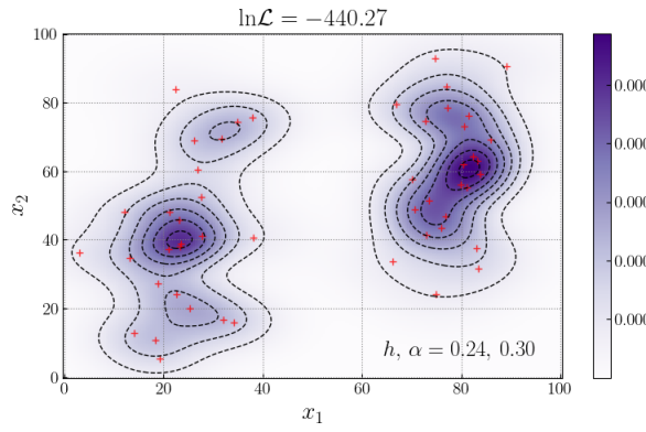
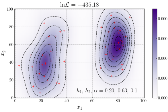
Figure 1: Verification of the multidimensional bandwidth optimization using mock data consisting of a mixture of two Gaussian components, represented by red $+$ symbols: contours and blue shading show the KDE in each case. Left: Adaptive KDE with an isotropic kernel (in standardized coordinates): the single bandwidth parameter $h$ and adaptive parameter $\alpha$ optimize the cross-validated likelihood. Right: Adaptive KDE with different optimized bandwidths $h_{1,2}$ for each coordinate.

To validate the multi-dimensional kernel optimization the new adaptive KDE method, we tested it using synthetic data comprising a bimodal Gaussian mixture. This dataset is useful for testing because the isotropic (spherical) kernel lacks the flexibility to capture its multimodality by using different bandwidths per parameter, even after standardizing the data to have the same variance in all dimensions.

We first apply adaptive KDE with an isotropic kernel in standardized coordinates, optimizing a single bandwidth parameter $h$ and adaptive parameter $\alpha$ to maximize the likelihood via leave-one-out cross-validation. However the resulting estimate, shown on the left of Fig. 1, is under-smoothed along one of the two dimensions, introducing excess variance and failing to represent the true distribution. Our improved KDE method allowing independently optimized bandwidths $h_{1}$ and $h_{2}$ for each coordinate better accommodates the anisotropic nature of the data, successfully recovering the bimodal Gaussian mixture, as shown in Fig. 1 (right), as well as significantly increasing the likelihood.

III Application to GWTC-3 data

We apply the reweighted adaptive KDE with multi-dimensional bandwidth optimization to the parameter estimation results LVK (2021a) of gravitational-wave observations cataloged in GWTC-3 Abbott et al. (2023a, c).

III.1 Event selection, parameter estimation and data cleaning

Following the approach in our earlier studies Sadiq et al. (2022, 2024a), we selected 69 BBH candidate events from GWTC-3, which have a false alarm rate below 1 per year. We excluded GW190814, an outlier event with an unusually low secondary mass ($m_{2}\simeq 2.6,M_{\odot}$, $q\simeq 0.11$), as its nature remains uncertain. This system could represent either a very massive neutron star or a light black hole, which is inconsistent with the primary BBH population we aim to analyze Abbott et al. (2020).

In LIGO-Virgo-KAGRA (LVK) catalog parameter estimation analyses, the prior over masses and $d_{L}$ is uniform over redshifted masses $m_{\{1,2\}z}=m_{\{1,2\}}(1+z)$ and over Euclidean volume Abbott et al. (2021a), thus is proportional to $(1+z)^{2}$ $d_{L}^{2}\mathrm{d}m_{1}\mathrm{d}m_{2}\mathrm{d}d_{L}$ (e.g. Callister (2021)). Samples reweighted to correspond to a “cosmological” prior uniform over comoving volume and source-frame time, though still uniform over $m_{z}$, are also available and are the basis of quoted event parameters Abbott et al. (2023a). We use the original samples and apply a factor proportional to the inverse prior $(1+z)^{-2}d_{L}^{-2}$ to our estimate of $p(m_{1}[,m_{2}],d_{L})$ in the reweighting step of our algorithm.

For two events with relatively low SNR, GW190719_215514 and GW190805_211137, we find a small number of PE samples at high distance which appear to represent the prior distribution, which is formally divergent towards large distance, rather than estimating the parameters of the detected merger. The expected (optimal) SNRs for these samples are unusually small. We compare the distances of PE samples with those of simulated signals (injections) which are subject to an expected network SNR cut of 6, as lower SNRs are considered “hopelessly” undetectable LVK (2023, 2021b). We thus exclude samples at higher distance than any injection with comparable masses (similar data cleaning was performed in Sadiq et al. (2024b)).

III.2 Selection effects

For the search sensitivity estimate or selection function, we employ an analytic approximant Lorenzo-Medina and Dent (2025) which accurately fits the probability of detection $p_{\mathrm{det}}$ at the 1 per year FAR threshold for injection (simulated signal) results released with the catalog LVK (2021b). The $p_{\mathrm{det}}$ approximant is a function of masses, effective inspiral spin $\chi_{\rm eff}$ Ajith et al. (2011) and luminosity distance, marginalizing over the sky direction, source orientation and spin orientations at given $\chi_{\rm eff}$. For our main results, we approximate $\chi_{\mathrm{eff}}$ to zero when evaluating the selection function for simplicity, motivated by findings in Abbott et al. (2023b) which support small effective spins for the observed BBH population.

We perform two separate analyses over masses and distance. In the first analysis, we reconstruct the population over primary mass and distance while assuming a power-law distribution of mass ratio $q=m_{2}/m_{1}$: here we compute $p_{\mathrm{det}}$ as a function of $m_{1}$ and $d_{L}$, while marginalizing over the secondary mass assuming a power-law distribution $\sim q^{\beta}$, see Fig. 2 (top), using the median estimate $\beta=1.26$ from the Truncated analysis of Abbott et al. (2021b), as a simple initial assumption.

In the second analysis, we reconstruct the 3d population over both component masses and distance: hence we evaluate $p_{\mathrm{det}}$ as a function of $m_{1}$, $m_{2}$, and $d_{L}$, see Fig. 2 (bottom).

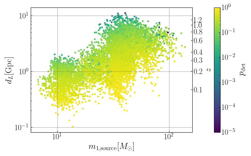
Figure 2: Detection probability $p_{\mathrm{det}}$ as a function of the primary mass $m_{1}$ and luminosity distance $d_{L}$ for parameter estimation samples from 69 BBH events in GWTC-3. The top panel assumes a power-law distribution for the mass ratio, $p(q)\propto q^{1.26}$, while the bottom panel uses posterior sample values of secondary mass $m_{2}$.

We conduct an additional check on the approximation of $\chi_{\rm eff}$ to zero by computing $p_{\mathrm{det}}$ based on the $\chi_{\mathrm{eff}}$ value of PE samples; see Fig. 10 for a direct comparison. Corresponding results are provided in Appendix A.

The fitted detection probability is a function of the redshifted masses $(1+z)m_{1,2}$ which describe the GW signal at the detectors. To relate the redshift to $d_{L}$ we assume a standard flat $\Lambda$CDM cosmology with $H_{0}=67.9\,$km/s/Mpc and $\Omega_{M}=0.3065$ Ade et al. (2016), as also used for LVK parameter estimation; changes in the assumed cosmology, particularly in $H_{0}$, would have minor effects on the reconstructed source mass spectrum.

In some regions of the parameter space, principally at high distance, $p_{\mathrm{det}}$ can become extremely small. Our KDE of detected events will also take low values in regions with small numbers of samples. In principle, our estimate of the astrophysical merger density is proportional to the ratio of the KDE to $p_{\mathrm{det}}$; however, in the limit of very small $p_{\mathrm{det}}$ this estimate will become numerically unstable. To mitigate or regularize this issue, we limit the range of $p_{\mathrm{det}}$ used in the analysis by replacing (capping) values below a predefined threshold $p_{\mathrm{det}}=0.1$ by the threshold value, as demonstrated in the context of LISA mock data in Sadiq et al. (2024b). As shown in Fig. 2, most samples have $p_{\mathrm{det}}$ values above or around $0.1$, but a small fraction have significantly lower values, particularly at larger distances or for higher primary masses. As a result of this capping or regularization we expect the rate estimate to be biased downwards, and eventually to approach zero, in regions with very small $p_{\mathrm{det}}$.

III.3 Limits on bandwidths

As described in Section II, we optimize the KDE hyperparameters using $k$-fold cross-validation with a likelihood figure of merit. We employ the Nelder-Mead optimizer to determine the optimal bandwidths $h_{k}$ for each dimension and the adaptive parameter $\alpha$: by default the allowed bandwidths for each dimension range between 0.01 and 1 (when considering standardized data).

In the two-dimensional analysis where a power-law assumption is applied to mass ratio, the distribution of optimized bandwidths over our bootstrap iterations is approximately Gaussian for both $m_{1}$ and $d_{L}$, and no iterations produce bandwidths smaller than 0.1.

However, in the three-dimensional analysis the optimized bandwidths for the $d_{L}$ dimension drop to $\lesssim\!0.1$ for a fraction of iterations. This behavior likely arises due to random clustering of samples at nearby $d_{L}$ values (see Appendix B). Density estimates for such small $d_{L}$ bandwidth values show several separate local maxima over distance or redshift; however, as this implies a large non-monotonic variation of the merger rate, we consider such behaviour astrophysically implausible. In addition, such wide rate variation contributes to excess variance in the iterative estimate.

To address this, in the 3d analysis we restrict the minimum bandwidth in the $d_{L}$ dimension (taking standardized data) to $0.3$, such that multimodal distributions over $d_{L}$ are largely eliminated. This has the potential drawback that the analysis would be unable to reconstruct rapid changes in the rate over distance or redshift. Thus, for completeness, we will provide results of the three-dimensional analysis without restrictions on the $d_{L}$ bandwidth in Appendix B.

IV Results

IV.1 2d primary mass vs. distance

We first apply our adaptive KDE with optimized non-isotropic kernels to reconstruct the BBH merger rate dependence on the primary mass and luminosity distance, assuming a power-law distribution over mass ratio when computing selection effects. Our KDE is implemented over $\log m_{1}$ and $d_{L}$: i.e., the Gaussian kernel takes a constant form specified by bandwidths $h_{m_{1}}$, $h_{d_{L}}$ in these coordinates. The resulting KDE is transformed to obtain a normalized density over $m_{1}$ and $d_{L}$. We then infer the rate density of arrival of GW events over this space by dividing by the estimated detection probability as in III.2 and multiplying by the number of detected events per observation time. We finally convert this KDE rate density to a cosmological merger rate density in units of comoving volume and source-frame time, as detailed in Appendix C.

The analysis uses 1100 iterative reweighting steps, where the first 100 iterations form a “burn-in” period and are discarded.

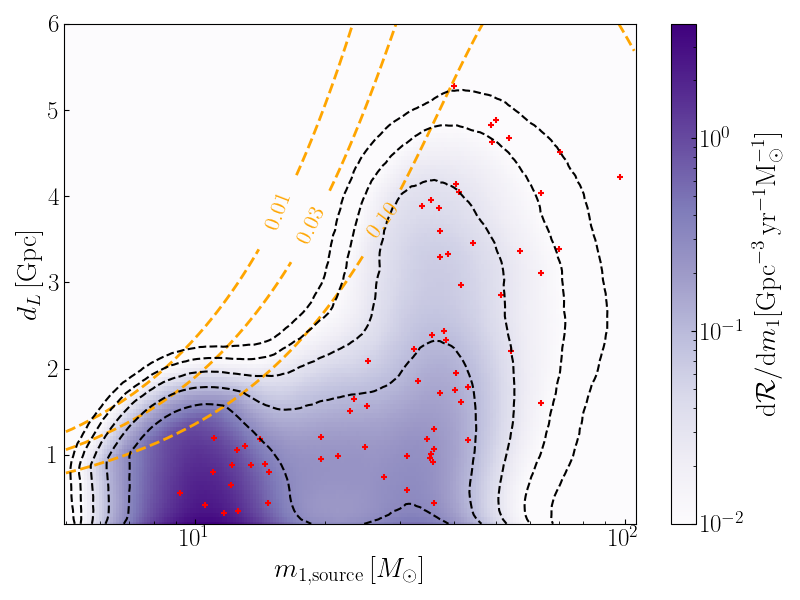
Figure 3: Rate density as a function of primary mass $m_{1}$ and luminosity distance $d_{L}$, assuming a power-law distribution for $m_{2}$. Red dots represent the medians of parameter estimation (PE) samples for BBH events, while the orange contours correspond to $p_{\mathrm{det}}$ levels. (One event, GW190805_211137, has a median $d_{L}\sim 7500$ Mpc outside the range of the plot.)

We plot the median rate density of the remaining 1000 iterations in Fig. 3. The median PE samples for all events lie within the $p_{\mathrm{det}}>0.1$ contour except one, GW190805_211137, with a median distance $\sim\!7500$ Mpc outside the plotted range. Thus, we may only expect an accurate or informative rate estimate within the $p_{\mathrm{det}}>0.1$ contour. For some ranges of primary mass the rate estimate may not even be valid up to this point, simply due to a low count of detected events: for instance for $m_{1}\lesssim 9\,M_{\odot}$ there is only a single detection, hence our rate estimate is effectively an extrapolation from higher mass events.

We observe a clear maximum around $m_{1}\simeq 10\,M_{\odot}$ which persists with approximately constant rate density up to the limit of validity of our reconstruction, $d_{L}\simeq 1.2\,$Gpc for this mass range. An underdensity just below $\sim\!20\,M_{\odot}$ again persists to the limit $p_{\mathrm{det}}\lesssim 0.1$. A second overdensity at roughly $m_{1}\simeq 35\,M_{\odot}$ again persists to the limit of detected events around $\sim\!4\,$Gpc, although with minor apparent variation in rate. Finally, the rate falls off at high mass $m_{2}\gtrsim 50\,M_{\odot}$: this falloff appears to be more rapid at low distance / redshift, with more support at distance $\sim\!3\,$Gpc, hinting at possible evolution of the high-mass end of the population.

To clearly display any evolution over redshift, we extract the rate density over $m_{1}$ at a sequence of $d_{L}$ or redshift values.

Figure 4: Merger rate density (median estimate) as a function of the primary mass $m_{1}$, with different curves representing redshift values indicated by color, assuming a power law distribution of mass ratio. Estimates at low mass are increasingly affected by selection bias towards high redshift.

We show median rate values in Fig. 4, and corresponding 90% uncertainty bands (applying cuts on large uncertainties) in Fig. 5.

Figure 5: Merger rate density as a function of primary mass with symmetric 90% confidence intervals, corresponding to the results shown in Fig. 4. Each curve shows a constant distance or redshift, shown by the color scale, with constant offsets applied for clarity. We only plot values where both (1) the 5th percentile is $>10^{-3}\times$ median, and (2) the 95th percentile is $\leq 200\times$ the median.

We observe two main apparent trends in Fig. 4: first, the height of the $10\,M_{\odot}$ peak, and the distribution below $30\,M_{\odot}$ as a whole, decreases rapidly at higher redshift; however this can be entirely attributed to “censorship” in this region due to the selection function. Second, the falloff at high mass ($>\!50\,M_{\odot}$) becomes shallower at higher redshift. Although this region is fully accessible to the detector network, Fig. 5 indicates that rate uncertainties are extremely large, which is not surprising given the very low statistics of detected high-mass events. Hence overall, this analysis is consistent with no evolution of the primary mass distribution.

IV.2 3d component masses vs. distance

We extend the analysis to three dimensions, imposing a constraint on the bandwidth in the $d_{L}$ dimension to be $\geq 0.3$ as discussed in III.3. The 3D analysis, as compared to the 2D case, removes the assumption of a power-law distribution for the mass ratio $m_{2}/m_{1}$ in selection effects, and allows us to investigate variations in the component mass distribution as a whole, including correlations. Analogously to previous cases we take a Gaussian kernel over $(\log m_{1},\log m_{2},d_{L})$.

Figure 6: BBH rate density as a function of component mass $m_{1}$ and luminosity distance $d_{L}$, for fixed $m_{2}$. Note that, for this plot only, we do not impose $m_{1}>m_{2}$ in displaying the KDE. The orange contours represent $p_{\mathrm{det}}$ at the given $m_{2}$ values. Red plus markers indicate the median of PE samples from GWTC-3.

From the 3D results, we compute rates for fixed values of $m_{2}$, as shown in Fig. 6 for $m_{2}=(10,35)\,M_{\odot}$, overplotting contours of $p_{\mathrm{det}}$. (Here, unlike for the rest of our results, we do not impose $m_{2}<m_{1}$: thus, these plots show a slice through the full 2-d component mass plane.) For $m_{2}=10\,M_{\odot}$, the overdensity around $m_{1}\simeq 10\,M_{\odot}$ persists up to the limit of detected events around $1\,$Gpc ($z\simeq 0.2$). For $m_{2}=35\,M_{\odot}$, the clear peak at $m_{1}\simeq 35\,M_{\odot}$ persists out to a distance $\sim 4\,$Gpc ($z\simeq 0.6$), however detected events fall somewhat short of the $p_{\mathrm{det}}=0.1$ contour, indicating that caution should be used when interpreting the reconstruction at such large distances. These features are roughly as expected from the 2D results shown in Fig. 3. Our comoving rate estimates also show an apparent increase at very low distance $d_{L}\lesssim 0.3\,$Gpc: this is an artefact of our choice to construct a KDE over $d_{L}$, as the kernels have nonzero support at zero distance. Hence, we do not expect the estimate to be valid at distances below the closest detected events ($\sim\!0.3\,$Gpc).

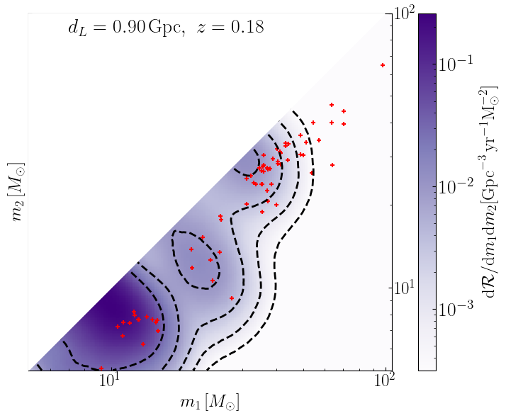
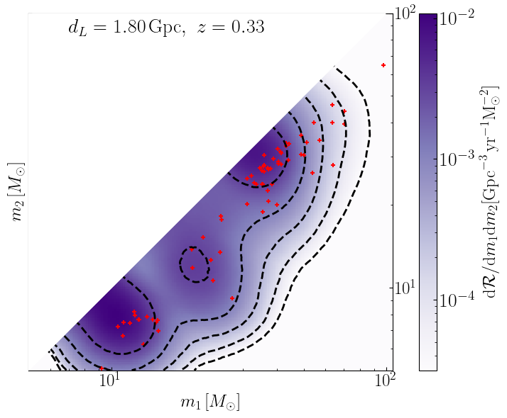
Figure 7: Rate density as a function of component masses at fixed luminosity distance or redshift values. The red dots represent the medians of parameter estimation (PE) samples.

We also select different $d_{L}$ values to plot the median rate over component masses, as in Fig. 7. The distribution at $0.9\,$Gpc shown in the upper plot is essentially unchanging for distances out to the detection horizon for $10\,M_{\odot}$ components; the lower plot suggests a shift towards apparent higher support for high BH masses at larger distances, however at $1.8\,$Gpc the principal change is again a suppression of the low-mass component due to selection effects (censorship).

Figure 8: Merger rate density (median estimate) as a function of the primary mass $m_{1}$, integrated over secondary mass, with different curves representing rates at redshift values indicated by color.

We further investigate potential evolution by taking several fixed $d_{L}$ (or $z$) values and integrating the joint rate over $m_{2}$ to obtain rate vs. primary mass $m_{1}$. Median rates are shown in Fig. 8 and rates with uncertainties in Fig. 9, showing similar trends to the 2D case where a power-law assumption was applied to $m_{2}$. Fig. 8 suggests a more visible trend towards shallower fall-off of the high mass distribution with increasing redshift; however, uncertainties remain extremely large for $m_{1}>50\,M_{\odot}$. Hence, again we do not see positive evidence for evolution.

Figure 9: Merger rate density as a function of the primary mass $m_{1}$, corresponding to the results shown in Fig. 8. Curves are defined as in Fig. 5.

Our alternative analysis using sample $\chi_{\mathrm{eff}}$ values to calculate $p_{\mathrm{det}}$ for the reweighting steps produces results, shown in Appendix A, extremely similar to our main analysis. The analysis with unrestricted $d_{L}$ bandwidth choice described in Appendix B, which might in principle be sensitive to rapid changes in rate over redshift, does not show features beyond those already noted, while having substantially larger uncertainties attributable to random sample fluctuations.

One further common feature of our rate estimates is that they slightly decrease with redshift, even well within the “horizon” of detected events where $p_{\mathrm{det}}\gtrsim 0.1$, except for the visible increase at high masses. This is in apparent contrast to some models of redshift evolution, for instance taking the comoving rate to vary proportional to $\mathcal{R}_{0}(1+z)^{\kappa}$ a generally positive, though small value of $\kappa$ is inferred Abbott et al. (2023b). However, non-parametric approaches to measuring evolution of the total BBH merger rate do not confirm a clear increase up to small redshifts $\lesssim 0.5$, some even showing a slight decrease Edelman et al. (2023); Callister and Farr (2024); Ray et al. (2023). Only for $z\gtrsim 0.6$ is an increasing trend visible: but as seen e.g. in Fig. 3, high-redshift estimates are driven almost entirely by high-mass events.

Such apparent discrepancies may require further investigation, as finite, though hopefully small, biases can arise, either in our method or in (semi-)parameterized models. On the KDE side the choice of a constant kernel (up to local adaptive scaling) in the logarithm of masses and in luminosity distance may cause some bias given the current low number of detections; we expect such biases to be reduced with higher event counts, as optimal bandwidths will become smaller and the exact choice of kernel becomes less important. Conversely parameterized evolution models, or even those allowing for more general $z$-dependence, typically assume specific functional forms for many parameters such as mass ratio and spins. Even when dependence on every parameter is described non-parametrically Edelman et al. (2023), any assumption that different parameters are uncorrelated is a significant restriction. Such assumptions may lead to biases in estimating the selection function or in individual event parameters, which may partially mimic an evolving rate, since rate estimates at different redshifts are informed by events with different intrinsic properties.

V Discussion

The detection of mass evolution with redshift using gravitational waves would have significant astrophysical implications, offering insights into the formation and evolution of compact binary systems over cosmic time and potentially helping to untangle different formation channels and environments. Recent studies using non-parametric or parametrized change-point methods with the same input data come to different conclusions. We use our non-parametric, data driven method, accounting for selection effects, to investigate this question and found no clear evidence, within the current limitations of observation selection effects and finite (low number) statistics.

The immediate implications from this study in are methodological rather than astrophysical. Given the low statistics of detections at masses above $\sim\!35\,M_{\odot}$ and non-detectability of low-mass BBH at redshifts above $z\sim 0.2$ in GWTC-3, our ability to infer anything about evolution of the BH mass spectrum is extremely limited. Apparent disagreements in previous inferences are probably due to different implicit assumptions about the behaviour of the population, inherent in the different methods employed. On the non-parametric side, methods may be prone to over-fit random fluctuations in observed event parameters, or underestimate uncertainties in regions with few (or zero!) detections. On the (semi-)parametric side, possible biases due to inaccurate model assumptions, for example on mass ratio and spins, are difficult to quantify directly. With increasing detector sensitivities and detection counts, different methods should converge, however meaningful probes of evolution may still be some way in the future. In particular, probing the high-mass end of the population will simply require significantly longer observing times: existing detectors are already sensitive out to moderately large redshift but statistics remain low due to the sheer rarity of mergers.

Overall, detecting mass evolution with redshift would provide a powerful tool to bridge gravitational-wave observations with broader astrophysical and cosmological phenomena. In future we will apply this method to the significantly larger set of observations expected from O4 and future runs, and further explore correlations with other parameters, such as spins.

Appendix A Spin dependence of selection function in reweighting

In our reweighting procedure, we incorporate selection effects into the parameter estimation samples. However, in our main study, these selection effects are estimated with $\chi_{\mathrm{eff}}=0$.

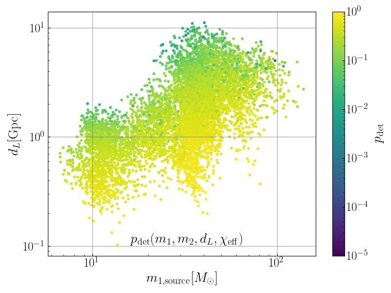
Figure 10: Detection probability $p_{\mathrm{det}}$ as a function of the primary mass $m_{1}$ and luminosity distance $d_{L}$ for GWTC-3 parameter estimation samples. Top: setting $\chi_{\mathrm{eff}}=0$ in evaluation of $p_{\mathrm{det}}$ (as in our main analysis). Bottom: using sample $\chi_{\mathrm{eff}}$ values in evaluation of $p_{\mathrm{det}}$.

Here, we investigate possible spin effects by using the PE sample $\chi_{\mathrm{eff}}$ values in evaluating $p_{\mathrm{det}}$ during the iterative reweighting procedure. We see generally small differences, as shown by the comparison in Fig. 10. In this analysis, we follow the same procedure as Sec. III.2 capping the maximum value of $p_{\mathrm{det}}$ at $0.1$ in order to regularize behaviour in regions with very small $p_{\mathrm{det}}$, and enforce a minimum bandwidth of $0.3$ over $d_{L}$. The resulting median rate estimates at fixed distance/redshift values shown in Fig. 11 are extremely similar to the main results which set $\chi_{\mathrm{eff}}=0$ in reweighting.

Figure 11: Alternative analysis using sample $\chi_{\mathrm{eff}}$ values to evaluate $p_{\mathrm{det}}$. Curves defined as in Fig. 13.

Appendix B Results with unrestricted bandwidth over distance

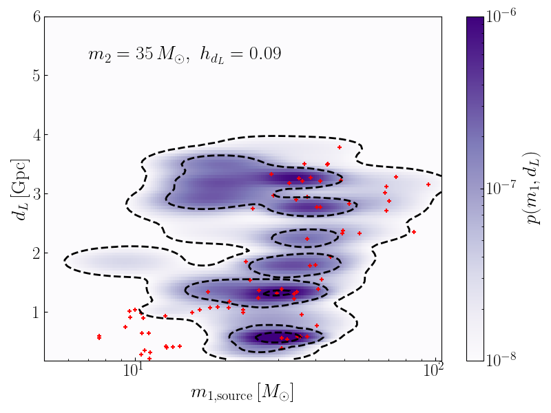
Figure 12: Density estimate for a single iteration with small optimal $d_{L}$ bandwidth, at a fixed $m_{2}$ slice, showing rapid variation in rate over distance/redshift. Red crosses indicate the samples selected in this iteration during the reweighting process.

We perform the same 3D analysis as described in the main text, but without imposing any lower limit on the optimized bandwidth in the $d_{L}$ dimension. Out of 1000 iterations, a few have an optimal bandwidth smaller than 0.1: Fig. 12 illustrates the effect of a small $d_{L}$ bandwidth on the KDE, showing a physically unrealistic strong multimodal variation over redshift. Overall, the results over all iterations remain largely unchanged, though with higher uncertainties, as illustrated in Figs. 13 and 14.

Figure 13: Merger rate density (median estimate) as a function of the primary mass $m_{1}$, integrated over secondary mass, with different curves representing rates at redshift values indicated by color. This analysis uses unrestricted bandwidth over $d_{L}$, in contrast to our main result.

Figure 14: Merger rate density as a function of the primary mass $m_{1}$ with uncertainties, corresponding to the results shown in Fig. 13. Curves are defined as in Fig. 5.

Appendix C Conversion to Cosmological Rate Density

As described in IV, we derive a KDE rate density, i.e. number density per observation time, over intrinsic parameters $\theta$ (here component mass) and luminosity distance, from the normalized KDE $p(\theta,d_{L})$ as

$$\frac{\mathrm{d}N}{\mathrm{d}\theta\mathrm{d}d_{L}\mathrm{d}t_{\mathrm{det}}}=\frac{p(\theta,d_{L})N_{\mathrm{obs}}}{p_{\mathrm{det}}(\theta,d_{L})T_{\mathrm{obs}}}.$$ (3)

We convert this to astrophysical rate density per comoving volume per source-frame time, $\mathrm{d}\mathcal{R}/\mathrm{d}\theta\equiv\mathrm{d}N/(\mathrm{d}\theta\mathrm{d}V_{c}\mathrm{d}t_{\mathrm{s}})$ via

$$\mathrm{d}\mathcal{R}=\frac{\mathrm{d}N}{\mathrm{d}d_{L}\mathrm{d}t_{\mathrm{det}}}\frac{\mathrm{d}t_{\mathrm{det}}}{\mathrm{d}t_{\mathrm{s}}}\frac{\mathrm{d}d_{L}}{\mathrm{d}z}\left(\frac{\mathrm{d}V_{c}}{\mathrm{d}z}\right)^{-1}.\vskip 1.42271pt$$ (4)

We have $\mathrm{d}t_{\mathrm{det}}/\mathrm{d}t_{\mathrm{s}}=1+z$ due to time dilation. Further, for flat $\Lambda$CDM cosmology we have (e.g. Hogg (1999))

$$\frac{\mathrm{d}V_{c}}{\mathrm{d}z}=4\pi d_{c}^{2}\frac{\mathrm{d}d_{c}}{\mathrm{d}z}=\frac{c}{H_{0}}\frac{4\pi d_{c}^{2}}{E(z)}\,,$$ (5)

where $d_{c}$ is the comoving line-of-sight distance

$$d_{c}=\frac{c}{H_{0}}\int_{0}^{z}\frac{dz^{\prime}}{E(z^{\prime})},\quad E(z)=\sqrt{\Omega_{m}(1+z)^{3}+\Omega_{\Lambda}}\,,$$ (6)

thus for the luminosity distance we have

$$d_{L}=(1+z)d_{c}\implies\frac{\mathrm{d}d_{L}}{\mathrm{d}z}=d_{c}+\frac{c}{H_{0}}\frac{(1+z)}{E(z)}.$$ (7)

References

- Abbott et al. (2016) B. P. Abbott et al. (LIGO Scientific, Virgo), Phys. Rev. Lett. 116, 061102 (2016), arXiv:1602.03837 [gr-qc] .
- Abbott et al. (2019a) B. P. Abbott et al. (LIGO Scientific, Virgo), Phys. Rev. X 9, 031040 (2019a), arXiv:1811.12907 [astro-ph.HE] .
- Abbott et al. (2021a) R. Abbott et al. (LIGO Scientific, Virgo), Phys. Rev. X 11, 021053 (2021a), arXiv:2010.14527 [gr-qc] .
- Abbott et al. (2024) R. Abbott et al. (LIGO Scientific, VIRGO), Phys. Rev. D 109, 022001 (2024), arXiv:2108.01045 [gr-qc] .
- Abbott et al. (2023a) R. Abbott et al. (KAGRA, VIRGO, LIGO Scientific), Phys. Rev. X 13, 041039 (2023a), arXiv:2111.03606 [gr-qc] .
- Aasi et al. (2015) J. Aasi et al. (LIGO Scientific), Class. Quant. Grav. 32, 074001 (2015), arXiv:1411.4547 [gr-qc] .
- Acernese et al. (2015) F. Acernese et al. (VIRGO), Class. Quant. Grav. 32, 024001 (2015), arXiv:1408.3978 [gr-qc] .
- Akutsu et al. (2021) T. Akutsu et al. (KAGRA), PTEP 2021, 05A101 (2021), arXiv:2005.05574 [physics.ins-det] .
- Abbott et al. (2019b) B. P. Abbott et al. (LIGO Scientific, Virgo), Astrophys. J. Lett. 882, L24 (2019b), arXiv:1811.12940 [astro-ph.HE] .
- Abbott et al. (2021b) R. Abbott et al. (LIGO Scientific, Virgo), Astrophys. J. Lett. 913, L7 (2021b), arXiv:2010.14533 [astro-ph.HE] .
- Abbott et al. (2023b) R. Abbott et al. (KAGRA, VIRGO, LIGO Scientific), Phys. Rev. X 13, 011048 (2023b), arXiv:2111.03634 [astro-ph.HE] .
- Madau and Dickinson (2014) P. Madau and M. Dickinson, Ann. Rev. Astron. Astrophys. 52, 415 (2014), arXiv:1403.0007 [astro-ph.CO] .
- Fishbach et al. (2018) M. Fishbach, D. E. Holz, and W. M. Farr, Astrophys. J. Lett. 863, L41 (2018), arXiv:1805.10270 [astro-ph.HE] .
- Callister et al. (2020) T. Callister, M. Fishbach, D. Holz, and W. Farr, Astrophys. J. Lett. 896, L32 (2020), arXiv:2003.12152 [astro-ph.HE] .
- Schiebelbein-Zwack and Fishbach (2024) A. Schiebelbein-Zwack and M. Fishbach, Astrophys. J. 970, 128 (2024), arXiv:2403.17156 [astro-ph.HE] .
- Tiwari and Fairhurst (2021) V. Tiwari and S. Fairhurst, Astrophys. J. Lett. 913, L19 (2021), arXiv:2011.04502 [astro-ph.HE] .
- Sadiq et al. (2022) J. Sadiq, T. Dent, and D. Wysocki, Phys. Rev. D 105, 123014 (2022), arXiv:2112.12659 [gr-qc] .
- Farah et al. (2023) A. M. Farah, B. Edelman, M. Zevin, M. Fishbach, J. M. Ezquiaga, B. Farr, and D. E. Holz, Astrophys. J. 955, 107 (2023), arXiv:2301.00834 [astro-ph.HE] .
- Talbot and Thrane (2018) C. Talbot and E. Thrane, Astrophys. J. 856, 173 (2018), arXiv:1801.02699 [astro-ph.HE] .
- Tiwari (2022) V. Tiwari, Astrophys. J. 928, 155 (2022), arXiv:2111.13991 [astro-ph.HE] .
- Farah et al. (2024) A. M. Farah, M. Fishbach, and D. E. Holz, Astrophys. J. 962, 69 (2024), arXiv:2308.05102 [astro-ph.HE] .
- Sadiq et al. (2024a) J. Sadiq, T. Dent, and M. Gieles, Astrophys. J. 960, 65 (2024a), arXiv:2307.12092 [astro-ph.HE] .
- Mapelli et al. (2019) M. Mapelli, N. Giacobbo, F. Santoliquido, and M. C. Artale, Mon. Not. Roy. Astron. Soc. 487, 2 (2019), arXiv:1902.01419 [astro-ph.HE] .
- van Son et al. (2022) L. A. C. van Son, S. E. de Mink, T. Callister, S. Justham, M. Renzo, T. Wagg, F. S. Broekgaarden, F. Kummer, R. Pakmor, and I. Mandel, Astrophys. J. 931, 17 (2022), arXiv:2110.01634 [astro-ph.HE] .
- Callister and Farr (2024) T. A. Callister and W. M. Farr, Phys. Rev. X 14, 021005 (2024), arXiv:2302.07289 [astro-ph.HE] .
- Edelman et al. (2023) B. Edelman, B. Farr, and Z. Doctor, Astrophys. J. 946, 16 (2023), arXiv:2210.12834 [astro-ph.HE] .
- Karathanasis et al. (2023) C. Karathanasis, S. Mukherjee, and S. Mastrogiovanni, Mon. Not. Roy. Astron. Soc. 523, 4539 (2023), arXiv:2204.13495 [astro-ph.CO] .
- Rinaldi et al. (2024) S. Rinaldi, W. Del Pozzo, M. Mapelli, A. Lorenzo-Medina, and T. Dent, Astron. Astrophys. 684, A204 (2024), arXiv:2310.03074 [astro-ph.HE] .
- Heinzel et al. (2024a) J. Heinzel, M. Mould, and S. Vitale, (2024a), arXiv:2406.16844 [astro-ph.HE] .
- Lalleman et al. (2025) M. Lalleman, K. Turbang, T. Callister, and N. van Remortel, (2025), arXiv:2501.10295 [astro-ph.HE] .
- Ivanova et al. (2013) N. Ivanova et al., Astron. Astrophys. Rev. 21, 59 (2013), arXiv:1209.4302 [astro-ph.HE] .
- van den Heuvel et al. (2017) E. P. J. van den Heuvel, S. F. Portegies Zwart, and S. E. de Mink, Mon. Not. Roy. Astron. Soc. 471, 4256 (2017), arXiv:1701.02355 [astro-ph.SR] .
- Gallegos-Garcia et al. (2021) M. Gallegos-Garcia, C. P. L. Berry, P. Marchant, and V. Kalogera, Astrophys. J. 922, 110 (2021), arXiv:2107.05702 [astro-ph.HE] .
- Mandel and de Mink (2016) I. Mandel and S. E. de Mink, Mon. Not. Roy. Astron. Soc. 458, 2634 (2016), arXiv:1601.00007 [astro-ph.HE] .
- de Mink and Mandel (2016) S. E. de Mink and I. Mandel, Mon. Not. Roy. Astron. Soc. 460, 3545 (2016), arXiv:1603.02291 [astro-ph.HE] .
- Marchant et al. (2016) P. Marchant, N. Langer, P. Podsiadlowski, T. M. Tauris, and T. J. Moriya, Astron. Astrophys. 588, A50 (2016), arXiv:1601.03718 [astro-ph.SR] .
- Downing et al. (2010) J. M. B. Downing, M. J. Benacquista, M. Giersz, and R. Spurzem, Mon. Not. Roy. Astron. Soc. 407, 1946 (2010), arXiv:0910.0546 [astro-ph.SR] .
- Rodriguez et al. (2015) C. L. Rodriguez, M. Morscher, B. Pattabiraman, S. Chatterjee, C.-J. Haster, and F. A. Rasio, Phys. Rev. Lett. 115, 051101 (2015), [Erratum: Phys.Rev.Lett. 116, 029901 (2016)], arXiv:1505.00792 [astro-ph.HE] .
- Rodriguez et al. (2019) C. L. Rodriguez, M. Zevin, P. Amaro-Seoane, S. Chatterjee, K. Kremer, F. A. Rasio, and C. S. Ye, Phys. Rev. D 100, 043027 (2019), arXiv:1906.10260 [astro-ph.HE] .
- Mapelli et al. (2022) M. Mapelli, Y. Bouffanais, F. Santoliquido, M. A. Sedda, and M. C. Artale, Mon. Not. Roy. Astron. Soc. 511, 5797 (2022), arXiv:2109.06222 [astro-ph.HE] .
- Miller and Lauburg (2009) M. C. Miller and V. M. Lauburg, Astrophys. J. 692, 917 (2009), arXiv:0804.2783 [astro-ph] .
- Antonini and Rasio (2016) F. Antonini and F. A. Rasio, Astrophys. J. 831, 187 (2016), arXiv:1606.04889 [astro-ph.HE] .
- Mckernan et al. (2018) B. Mckernan et al., Astrophys. J. 866, 66 (2018), arXiv:1702.07818 [astro-ph.HE] .
- Stone et al. (2017) N. C. Stone, B. D. Metzger, and Z. Haiman, Mon. Not. Roy. Astron. Soc. 464, 946 (2017), arXiv:1602.04226 [astro-ph.GA] .
- Silsbee and Tremaine (2017) K. Silsbee and S. Tremaine, Astrophys. J. 836, 39 (2017), arXiv:1608.07642 [astro-ph.HE] .
- Bavera et al. (2021) S. S. Bavera et al., Astron. Astrophys. 647, A153 (2021), arXiv:2010.16333 [astro-ph.HE] .
- Bavera et al. (2022) S. S. Bavera, M. Fishbach, M. Zevin, E. Zapartas, and T. Fragos, Astron. Astrophys. 665, A59 (2022), arXiv:2204.02619 [astro-ph.HE] .
- Zevin et al. (2021) M. Zevin, S. S. Bavera, C. P. L. Berry, V. Kalogera, T. Fragos, P. Marchant, C. L. Rodriguez, F. Antonini, D. E. Holz, and C. Pankow, Astrophys. J. 910, 152 (2021), arXiv:2011.10057 [astro-ph.HE] .
- Zevin and Bavera (2022) M. Zevin and S. S. Bavera, Astrophys. J. 933, 86 (2022), arXiv:2203.02515 [astro-ph.HE] .
- Broekgaarden et al. (2022) F. S. Broekgaarden, S. Stevenson, and E. Thrane, Astrophys. J. 938, 45 (2022), arXiv:2205.01693 [astro-ph.HE] .
- Fuller and Ma (2019) J. Fuller and L. Ma, Astrophys. J. Lett. 881, L1 (2019), arXiv:1907.03714 [astro-ph.SR] .
- Bavera et al. (2020) S. S. Bavera, T. Fragos, Y. Qin, E. Zapartas, C. J. Neijssel, I. Mandel, A. Batta, S. M. Gaebel, C. Kimball, and S. Stevenson, Astron. Astrophys. 635, A97 (2020), arXiv:1906.12257 [astro-ph.HE] .
- Fuller and Lu (2022) J. Fuller and W. Lu, Mon. Not. Roy. Astron. Soc. 511, 3951 (2022), arXiv:2201.08407 [astro-ph.HE] .
- Barkat et al. (1967) Z. Barkat, G. Rakavy, and N. Sack, Phys. Rev. Lett. 18, 379 (1967).
- Woosley (2017) S. E. Woosley, Astrophys. J. 836, 244 (2017), arXiv:1608.08939 [astro-ph.HE] .
- Tanikawa et al. (2022) A. Tanikawa, M. Giersz, and M. A. Sedda, Mon. Not. Roy. Astron. Soc. 515, 4038 (2022), arXiv:2103.14185 [astro-ph.HE] .
- Afroz and Mukherjee (2024) S. Afroz and S. Mukherjee, (2024), arXiv:2411.07304 [astro-ph.HE] .
- Heinzel et al. (2024b) J. Heinzel, M. Mould, S. Álvarez-López, and S. Vitale, (2024b), arXiv:2406.16813 [astro-ph.HE] .
- Ng et al. (2024) T. C. K. Ng, S. Rinaldi, and O. A. Hannuksela, (2024), arXiv:2410.23541 [gr-qc] .
- Fabbri et al. (2025) C. M. Fabbri, D. Gerosa, A. Santini, M. Mould, A. Toubiana, and J. Gair, (2025), arXiv:2501.17233 [astro-ph.HE] .
- Sadiq et al. (2024b) J. Sadiq, K. Dey, T. Dent, and E. Barausse, (2024b), arXiv:2410.17056 [gr-qc] .
- Lorenzo-Medina and Dent (2025) A. Lorenzo-Medina and T. Dent, Class. Quant. Grav. 42, 045008 (2025), arXiv:2408.13383 [gr-qc] .
- Odland (2018) T. Odland, “tommyod/kdepy: Kernel density estimation in python,” (2018), https://doi.org/10.5281/zenodo.2392268.
- Note (1) Standardization also changes the likelihood figure of merit, but only by a constant for a given data set.
- LVK (2021a) LVK, “GWTC-3: Parameter estimation data release,” (2021a), https://doi.org/10.5281/zenodo.5546663.
- Abbott et al. (2023c) R. Abbott et al. (KAGRA, VIRGO, LIGO Scientific), Astrophys. J. Suppl. 267, 29 (2023c), arXiv:2302.03676 [gr-qc] .
- Abbott et al. (2020) R. Abbott et al. (LIGO Scientific, Virgo), Astrophys. J. Lett. 896, L44 (2020), arXiv:2006.12611 [astro-ph.HE] .
- Callister (2021) T. Callister, (2021), arXiv:2104.09508 [gr-qc] .
- LVK (2023) LVK, “Gwtc-3: Compact binary coalescences observed by ligo and virgo during the second part of the third observing run — O3 search sensitivity estimates,” (2023), https://doi.org/10.5281/zenodo.7890437.
- LVK (2021b) LVK, “GWTC-3: O1+O2+O3 Search Sensitivity Estimates,” (2021b), https://doi.org/10.5281/zenodo.5636816.
- Ajith et al. (2011) P. Ajith et al., Phys. Rev. Lett. 106, 241101 (2011), arXiv:0909.2867 [gr-qc] .
- Ade et al. (2016) P. A. R. Ade et al. (Planck), Astron. Astrophys. 594, A13 (2016), arXiv:1502.01589 [astro-ph.CO] .
- Ray et al. (2023) A. Ray, I. Magaña Hernandez, S. Mohite, J. Creighton, and S. Kapadia, Astrophys. J. 957, 37 (2023), arXiv:2304.08046 [gr-qc] .
- Hogg (1999) D. W. Hogg, (1999), arXiv:astro-ph/9905116 .