On the distance to the black hole X-ray binary Swift J1727.8$-$1613

Abstract

We review the existing distance estimates to the black hole X-ray binary Swift J1727.8$-$1613 (catalog ) with a discussion of the accuracies and caveats of the associated methodologies. As part of this, we present new line-of-sight H i absorption spectra captured using the MeerKAT radio telescope. We estimate a maximum radial velocity with respect to the local standard of rest of $24.8\pm 2.8$ km s^-1, which is significantly lower than that found towards an extragalactic reference source. Given the location of Swift J1727.8$-$1613 at Galactic longitude and latitude $(l,b)\approx(8.6^{\circ},10.3^{\circ})$, we explore the feasibility of the H i absorption method. From this we derive a near kinematic distance of $d_{\rm{near}}=3.6\pm 0.3\,({stat})\pm 2.3\,({sys})$ kpc as lower bound for the distance to Swift J1727.8$-$1613. We compare our results with those derived from different distance determination methods including the use of colour excess or reddening along the line of sight, which we constrain to $E(B\!-\!V)=0.37\pm 0.01\,({stat})\pm 0.025\,({sys})$ using near-UV spectra. By combining this with donor star magnitudes reported by Mata Sánchez et al. (2025), we suggest an increased distance of $5.5^{+1.4}_{-1.1}$ kpc, which would imply a natal kick velocity of $190\pm 30$ km s^-1.

revtex4-1.clsrevtex4-2.cls

1 Introduction

Distance measurement is important for all objects. In studying Galactic low-mass X-ray binaries (XRBs), accurate distances allow for better estimation of parameters such as the peak Eddington luminosity ($L_{\rm{Edd}}$) fraction (ELF) and jet parameters including physical size scales, inclination angles, and speeds.

Reliably measuring the distance to newly discovered XRBs can be challenging. For instance, as the accretion processes of low-mass XRBs evolve, the system’s luminosity can fluctuate, often in and out of detectable levels. This inconsistent detectability can preclude the measurements required for accurate distance determination.

1.1 Distance methods

Distance determination techniques for XRBs can be broadly summarised as methods that use either astrometry or kinematics, observations of the donor star or X-ray source, or propagation effects.

1.1.1 Astrometry and kinematics

High-significance XRB parallax measurements with Gaia (Gandhi et al., 2019; Atri et al., 2019; Arnason et al., 2021) or very long baseline interferometry (VLBI) at radio wavelengths (e.g.; Miller-Jones et al., 2009; Reid et al., 2011; Atri et al., 2020; Miller-Jones et al., 2021; Reid & Miller-Jones, 2023) are the gold standard for measuring distances. However, radio parallaxes can be impeded by line-of-sight scatter broadening for XRBs located in the Galactic Plane (GP). Given the typical kpc distances of XRBs, sub-milliarcsecond precision is required (Tetarenko et al., 2016).

Alternatively, kinematic distance methodologies use measured proper motions and velocities predicted using the Galactic rotation model to infer the most likely distance. In some circumstances, these have been shown to have similar if not better accuracy than parallax (Reid, 2022) and useful for XRBs (e.g.; Dhawan et al., 2007; Reid & Miller-Jones, 2023).

1.1.2 Stellar and X-ray observations

One can use optical spectroscopy of the XRB donor star to estimate the distance (e.g.; Dubus et al., 2001; Jonker & Nelemans, 2004; Charles et al., 2019). With measured values for the donor star’s absolute and apparent magnitudes and the line-of-sight extinction along the line of sight, one can then use the distance modulus (e.g.; Mata Sánchez et al., 2024, 2025)

$$d=10^{(m-M-A+5)/5}$$ (1)

where $d$ is the distance, $m$ is the apparent magnitude, $M$ is the absolute magnitude, and $A$ is the extinction.

Obscuration of optical light is pronounced for targets residing in the GP due to increased interstellar dust, making donor stars difficult to identify, and introducing additional uncertainty to the distance modulus equation. However, for targets outside the GP, extinction can be harder to estimate accurately. We use and discuss this method in Section 4.2.

X-ray luminosities of XRB outbursts during soft-to-hard and hard-to-intermediate state transitions have been observed to occur at somewhat consistent ELFs, albeit with factor of $\sim\!3$ scatter in these measurements (Kalemci et al., 2013; Tetarenko et al., 2016; Vahdat Motlagh et al., 2019). X-ray studies during these transitions allow the comparison of measured and expected intrinsic luminosities, enabling the estimation of distance (e.g.; Abdulghani et al., 2024).

1.1.3 Propagation

By analysing the time delays and intensities of X-rays that had been produced by flares and subsequently scattered off intervening interstellar dust clouds, one can reconstruct the XRB outburst light curve and determine the distance to the source (e.g.; Heinz et al., 2015; Beardmore et al., 2016; Lamer et al., 2021).

X-ray absorption features in observed spectra can be used to measure the hydrogen column density, $N_{\rm{H}}$. When coupled with hydrogen distribution models one can infer the distance to the source. We discuss this further in Section 4.2.

The relation between the colour excess or reddening, $E(B\!-\!V)$, and extinction can also be used to inform distance modulus calculations (e.g.; Schlafly & Finkbeiner, 2011). The inverse relation between $E(B\!-\!V)$ and the distance therefore allows constraints on one to constrain the other. $E(B\!-\!V)$ can be estimated using various relations between it and interstellar absorption lines (e.g.; Munari & Zwitter, 1997; Wallerstein et al., 2007), or from near-UV observations, as used in Sections 2.2 and 3.2. $E(B\!-\!V)$ has also been determined from 2-dimensional (2D; e.g.; Schlegel et al., 1998; Chiang, 2023) and 3-dimensional (3D; e.g.; Green et al., 2019; Edenhofer et al., 2024) Galactic dust maps.

Lastly, line-of-sight H i absorption has long been used as an XRB distance estimator (e.g.; Dickey, 1983; Lockman et al., 2007; Chauhan et al., 2019, 2021). We have also applied this method in Sections 2.1 and 3.1.

MJD	Observation	Observation	Exposure	Centre	Total	Channel	J1727
	start date	start time	time	frequency	bandwidth	width	peak flux density
	(dd-mm-yyyy)	(hh:mm:ss)	(mm:ss)	(MHz)	(MHz)	(kHz)	(mJy)
60183	27-08-2023	15:27:59.6	14:55.6	1283.9869	856	26.123	$49.7\pm 0.2$
60193	06-09-2023	15:06:32.1	14:56.9	1419.9984	107	3.265	$97.5\pm 0.4$
60231	14-10-2023	12:40:20.2	14:55.6	1283.9869	856	26.123	$836.6\pm 2.3$
60233	16-10-2023	15:50:13.8	14:56.9	1419.9984	107	3.265	$104.3\pm 0.4$

Table 1: A summary of MeerKAT observation parameters. All times are in Coordinated Universal Time (UTC). The uncertainties on the peak flux densities are the root-mean-square (RMS) noise in the continuum image of the J1727 field.

1.1.4 H I absorption

H i absorption occurs when clouds of neutral hydrogen along the line of sight absorb the broadband continuum emission produced by the target at the H i frequency in their rest frame. These clouds move with different velocities relative to us along the line of sight, due to the rotation of the Milky Way, as well as other effects such as non-circular streaming motions that we assume to be minimal. The more clouds that are intersected by the line of sight, the more H i absorption features that are imprinted at different frequencies on the observed radio spectrum. One benefit of H i absorption over parallax is that the required data can be gathered within a much shorter timeframe; a single observation can suffice should the observed source be particularly bright.

Using the Milky Way rotation curve, the Doppler-shifted frequencies can be converted into local standard of rest (LSR) velocities. The maximum velocity occurs at the tangent point, where the rotational velocity is entirely along the line of sight. Identical velocities are seen either side of this maximum, giving rise to an ambiguity in mapping observed absorption velocities to distances within the solar circle. A maximum observed velocity that is less than the tangent point velocity could correspond to a near kinematic distance before the tangent point, or a far kinematic distance beyond the tangent point (e.g.; Wenger et al., 2018, Figure 4).

To resolve this kinematic distance ambiguity, one must observe the target but also at least one extragalactic reference source close enough to the target in the sky such that any differences in the anticipated H i distributions along the lines of sight are minimised. The emission from the reference source will have passed through all Galactic H i clouds along the line of sight, with clouds outside the solar circle imprinting absorption velocities of the opposite sign. Any absorption present in the reference spectrum but absent in the target spectrum then allows us to place an upper limit on the distance. Further to this, observations of two-sided relativistic jets can be used to give a maximum distance to a source.

1.2 Swift J1727.8$-$1613

Swift J1727.8$-$1613 (J1727), located at $(l,b)=(8.641502^{\circ},10.254899^{\circ})$, was first detected as an X-ray transient on 24 August 2023 (Negoro et al., 2023), after which bright radio emission was observed within a couple of days (Miller-Jones et al., 2023b), which continued to brighten through early September (Bright et al., 2023). Analysis of observations in late August and early September revealed a bright core and a large two-sided, asymmetrical jet (Wood et al., 2024). Radio monitoring in early October suggested radio quenching and subsequent flaring (Miller-Jones et al., 2023a).

This event was deemed a low-mass XRB outburst (Castro-Tirado et al., 2023), and its high radio brightness made J1727 a suitable target for H i absorption measurements. Since then, the compact object has been dynamically confirmed to be a black hole (BH) (Mata Sánchez et al., 2025, MS24b hereafter).

Abdulghani et al. (2024) provided an initial distance estimate of $1.52^{+0.85}_{-0.61}$ kpc from the ELF method mentioned in Section 1.1.2. The authors concede that this particular distance estimate may be underestimated by up to $\sim\!70\%$. Mata Sánchez et al. (2024, MS24a hereafter) suggested a distance of $2.7\pm 0.3$ kpc. MS24b classified the donor star type as K3/4V and updated the distance to $3.4\pm 0.3$ kpc.

The Gaia optical counterpart for Swift J1727.8$-$1613 currently has proper motion but no parallax. A VLBI radio parallax will not be possible, as the XRB has already returned to the quiescent state.

In Section 2 we detail the methods used and data obtained. In Section 3 we present our H i absorption and near-UV spectra. In Section 4 we discuss the interpretation of the H i absorption results, their use in estimating the kinematic distance, and the associated caveats. We extend this discussion to compare our result with others published to date, augment this using our near-UV results, and explore the implications of the resulting distance estimate. In Section 5 we present our best estimate of the distance to J1727.

2 Observations and Data Reduction

2.1 MeerKAT radio data

We observed J1727 as part of the The hunt for dynamic and explosive radio transients with MeerKAT (ThunderKAT; Fender et al., 2016) large survey project and its successor, X-KAT (PI Fender).

We conducted 1–2 GHz (L-band) radio observations of the J1727 field using the South African Square Kilometre Array precursor radio telescope, MeerKAT (Camilo, 2018), between 27 August and 16 October 2023. Our measured flux densities for J1727 were in the range 50–837 mJy due to radio flaring of the source. Further details of these observations are provided in Table 1.

All observations were performed with the L-band receiver; two using MeerKAT’s standard “32k” mode, and two using the “32k zoom” mode, hereafter referred to as “32k-S” and “32k-Z” respectively. While each mode contains 32,768 channels, the 32k-Z mode has channel bandwidths that are eight times smaller and thus provides an eight-fold increase in frequency resolution. We alternated our observation scans between J1727 and the phase calibrator, PKS J1733$-$1304 (J1733 hereafter), with a single scan of the bandpass and flux calibrator J1939$-$6342 in each observation.

Having obtained MeerKAT observations of J1727 during which it was sufficiently bright at 1.4 GHz (i.e., $\gtrsim\!50$ mJy), we compute H i absorption spectra by processing the radio data to create a radio spectrum that includes the frequency of the H i spectral line, $f_{\textsc{Hi}}=1420.30575177$. We convert frequency to line-of-sight LSR velocity by combining the Doppler shift with the Milky Way rotation curve. We then use the maximum positive or negative velocity observed in the resulting spectra to generate estimates of the kinematic distance via the source code for the Kinematic Distance Calculation Tool^, (KDCT; Wenger, 2018).

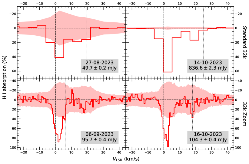
Figure 1: Our H i absorption spectra along of the line of sight towards J1727. The top two plots are the 32k-S spectra, and the bottom two plots are the 32k-Z spectra, with LSR velocity bin widths that are 5.6 and 0.7 km s^-1 wide respectively. The dashed lines indicate the origins of the x- and y-axis. The y-axis represents the residuals after subtracting the continuum emission from the data, with $3\sigma$ uncertainties indicated by the shaded areas, both of which are presented as a percentage of the continuum flux density of the source. The vertical dotted lines indicate the maximum velocity taken as the mid-point of the bin at which significant ($>\!3\sigma$) absorption is observed. In chronological order, these maximum velocities are $19.2\pm 2.8$, $6.1\pm 0.4$, $24.8\pm 2.8$, and $18.0\pm 0.4$ km s^-1. The significantly greater SNR of the 14-10-2023 spectrum meant we were able to observe significant ($>\!3\sigma$) H i absorption to greater velocities than observed in the 32k-Z spectra.

2.1.1 Reference source selection

Due to the lack of bright ($\gtrsim\!50$ mJy) extragalactic background sources in the field i.e., within $1^{\circ}$ of J1727, we used the sufficiently bright ($S_{0}\approx 6$ Jy) phase calibrator J1733 to derive our reference H i absorption spectra. With J1733 located at $(l,b)\approx(12.03^{\circ},10.81^{\circ})$, the two fields are only $3.4^{\circ}$ apart, primarily in Galactic longitude. As J1733 is extragalactic, observations allow us to probe the full set of H i clouds along a nearby line of sight (see also Section 4.1.2 regarding H i scale height).

2.1.2 Data reduction

We undertook all data reduction on the Ilifu research cloud infrastructure managed by the Inter-University Institute for Data Intensive Astronomy (IDIA). To streamline the processing of our H i data, we used the ThunderKAT H i Pipeline. Simultaneously, we used CARTA (Cube Analysis and Rendering Tool for Astronomy; Comrie et al., 2021) to interrogate the data.

There are three stages of the pipeline, each with its own bash script that employs several Python scripts.

At a high level, the first stage of the pipeline uses CASA (Common Astronomy Software Applications; CASA Team et al., 2022) to retrieve the data for specified fields from the full observation measurement set and create separate files for each source. The pipeline then undoes previously applied flags to to ensure H i spectral lines are not erroneously flagged as radio-frequency interference. The measurement set for each field is then converted into the fits format required for the Miriad software (Sault et al., 1995) used in the next stage.

The second and most computationally intensive stage begins with data pre-processing, and a region is defined to search for the position of the peak continuum emission. The target and calibrators’ fields are defined, the reference antenna is set, and basic flagging is done. The H i spectral line frequency is added to the header information to convert frequency to velocity. Bandpass and gain calibrations are applied to the target field, and spectral cubes are made and cleaned for the target and defined reference source(s). A second-order polynomial is then fitted to the broadband radio continuum emission of each source and subtracted in frequency space to remove the continuum emission. The resulting residuals are used to create image cubes for each source, from which the spectra are extracted and written to ASCII files, ready for the final stage.

The third stage plots the target and reference spectra. The noise in each channel is used to give an estimation of absorption uncertainties in the velocity bins. In the event that there are multiple target or reference spectra to be combined, these are “stacked” to create weighted mean spectra and increase the signal-to-noise ratio (SNR). The absorption in each velocity bin is calculated from each spectrum weighted according to the inverse square of the noise.

2.2 Hubble Space Telescope near-UV spectroscopy

We obtained high resolution near-UV spectroscopy with the Space Telescope Imaging Spectrograph (STIS; Woodgate et al., 1998) aboard the Hubble Space Telescope (HST) in early October 2023 ($\rm MJD\sim 60219$) during the outburst (program ID 16489; Castro Segura et al., 2020). We used E230M gratings with 200 s followed by 220 s exposures at the central wavelengths 1978 Å and 2707 Å respectively to cover the region $\lambda\lambda\simeq 1800$–$3200$ Å with a resolving power of $R=30,\!000$. The data were reduced using the HST pipeline calstis.

These observations provide an alternative and generally more accurate method to estimate $E(B\!-\!V)$ and subsequently the distance to J1727 as detailed in Sections 3.2 and 4.3 respectively.

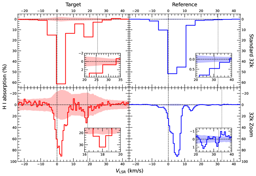
Figure 2: A consolidated view of the H i spectra for both the target, J1727 (red, left), and our reference source, J1733 (blue, right). We observed no significant ($>\!3\sigma$) absorption outside the velocities chosen as the x-axis range. The y-axis represents the H i absorption percentage. The dashed lines indicate the x- and y-axes origins. The vertical dotted lines indicate the maximum velocity at which significant absorption is observed. For J1727, these are $24.8\pm 2.8$ and $18.7\pm 0.4$ km s^-1. For J1733, these are $30.4\pm 2.8$ and $32.7\pm 0.4$ km s^-1. The top-left plot is the 32k-S spectrum for J1727 from 14-10-2023, while the bottom-left plot is the mean weighted J1727 spectrum achieved by combining both 32k-Z spectra from Figure 1. We generated the 32k-Z (32k-S) spectra for J1733 from observations on 06-09-2023 (14-10-2023) with the peak J1733 flux density measured to be $6.1\pm 0.1$ Jy ($6.0\pm 0.1$ Jy), providing the significantly greater SNR compared to that of the J1727 observations.

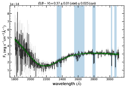
Figure 3: The near-UV spectrum of J1727 as seen by HST/STIS (black), with a reddened power-law fit to the data (green) (Castro Segura et al. in prep.) The uncertainty around the fit is indicated as a shaded region. The vertical shaded regions were masked during the fit to avoid Fe and Mg lines that may influence the fit.

3 Results

3.1 Radio

3.1.1 High resolution 32k zoom mode

Both H i spectra from our two 32k-Z observations are displayed in the bottom two plots of Figure 1. Significant ($>\!3\sigma$) H i absorption towards J1727 is observed out to an estimated maximum LSR velocity $v_{\rm{LSR}}=18.7\pm 0.4$ km s^-1 as shown in the inset for the the mean weighted 32k-Z spectrum at the bottom-left of Figure 2, using half the bin width as the velocity uncertainty. The maximum absorption is observed to be $\approx 90\%$.

3.1.2 Standard 32k mode

The effect of J1727’s variable luminosities over the period of observations is seen in the differing SNR between our H i spectra from 27-08-2023 and 14-10-2023 shown in Figure 1. For 14-10-2023 we measured a J1727 peak flux density that was more than eight times greater than either of our 32k-Z observations due to radio flaring, as observed by Miller-Jones et al. (2023a). The 14-10-2023 spectrum shows H i absorption at greater velocities than the 32k-Z spectra, albeit with greater bin widths. We therefore update our estimate of the maximum velocity of significant H i absorption towards J1727 to $v_{\rm{LSR}}=24.8\pm 2.8$ km s^-1 as seen in the top-left inset in Figure 2. The maximum absorption is observed to be $\approx 61\%$ for the 32k-S spectra, which is smaller than that of the 32k-Z spectra as the absorption is averaged over the wider velocity bin width.

3.1.3 Reference source

Figure 2 compares H i absorption spectra towards J1727 and J1733. The latter is consistently much brighter, with flux densities exceeding 6 Jy. It also exhibits H i absorption to greater velocities (i.e., $32.7\pm 0.4$ km s^-1 in the 32k-Z spectrum), which is in line with J1733 being extragalactic. With an extragalactic point of comparison that is nearby in terms of sky location and with H i absorption to greater velocities, we infer that J1727 is closer than the tangent point, and use the near kinematic distance as a lower limit.

3.2 Near-UV

We determined the line of sight extinction to J1727 using the Cardelli et al. (1989) reddening law to fit a reddened power-law representing the outer accretion disk to the near-UV spectrum as displayed in Figure 3. To estimate the errors we performed a Monte Carlo simulation yielding $E(B\!-\!V)=0.37\pm 0.01\,({stat})\pm 0.025\,({sys})$, corresponding to $A_{V}=R_{V}\,E(B\!-\!V)\simeq 1.00$ for $R_{V}=3.1$.

4 Discussion

4.1 Kinematic distance constraint

Absorption features in the final H i spectra informed our use of the KDCT to generate kinematic distance estimates. We clearly observe greater velocities towards J1733 than J1727, as shown in Figure 2.

We used our maximum H i absorption velocity and its uncertainty as inputs to the KDCT (Wenger et al., 2018), using their Method C and applying the revised solar motion parameters from Reid et al. (2014) and the rotation curve from Reid et al. (2019). The total revised LSR velocity uncertainty includes measurement and systematic uncertainties such as non-circular streaming motions.

We amended the KDCT source code to resample the input and Galactic rotation curve parameters $10^{7}$ times to minimise Monte Carlo error. Results include Monte Carlo samples of $d_{\rm{near}}$, $d_{\rm{tan}}$ (tangent point kinematic distance), and $v_{\rm{LSR,tan}}$ (tangent point LSR velocity). We estimate and report the median values as best estimates and the boundaries of the highest density 68% interval as the uncertainties on these quantities. We repeated this process using inputs from 32k-Z and 32k-S H i absorption spectra.

The quantities of $d_{\rm{tan}}$ and $v_{\rm{LSR,tan}}$ depend only on the source location. Therefore, we used $(l,b)=(8.641502^{\circ},10.254899^{\circ})$ for J1727 to estimate $d_{\rm{tan}}=8.20\pm 0.03$ kpc and $v_{\rm{LSR,tan}}=93.9\pm 3.3$ km s^-1. As $d_{\rm{near}}$ depends on the input velocity, we use our higher-SNR result of $24.8\pm 2.8$ km s^-1 from our 32k-S spectra to estimate $d_{\rm{near}}=3.6\pm 0.3$ kpc.

4.1.1 Caveats

J1727 has a longitude close to the Galactic Centre (GC) and a relatively high Galactic latitude, leading to larger systematic uncertainties on the kinematic distance.

Regions within 15 degrees in Galactic longitude from the GC feature increased H i emission from the GC (Kalberla & Kerp, 2009), which leads to higher sky temperatures around the H i line and hence increased uncertainty in each spectral channel. At these longitudes, the motion of objects intersected by the line of sight is mostly perpendicular to the line of sight. Distances are thus inferred from a smaller spread in circular rotation velocities and subject to larger uncertainties, and so this region was excised from the study of Wenger et al. (2018).

More recently, Hunter et al. (2024) conducted numerical 2D hydrodynamical simulations to account for potential causes of Milky Way deviations from axisymmetry and gas cloud deviations from the circular rotation curve. The authors categorise these deviations into: (i) random fluctuations around the average streaming motions that do not change the average velocity; and (ii) systematic changes in streaming velocity due to non-axisymmetry, such as spiral arms and the Galactic bar. The authors then define regions of their simulated Milky Way Galaxy where the discrepancy between the kinematic and true distance is significant ($>\!27\%$). Within $2\!<\!d\!<\!5$ kpc, the longitude for J1727 appears to correspond to a median absolute relative kinematic distance error of $|d_{\rm{k}}-d_{\rm{true}}|/d_{\rm{true}}\approx 63\%$. For $5\!<\!d\!<\!10$ kpc, this error reduces to approximately $12\pm 8\%$. We use the greater 63% error above to expand the $1\sigma$ uncertainty on our measured kinematic distance, which becomes $3.6\pm 0.3\,({stat})\pm 2.3\,({sys})$ kpc. Having used 2D simulations, Hunter et al. (2024) assume that the gas is integrated along the $z$-axis (vertically), and that the acceleration of the gas due to the Galactic potential is computed as if the gas lies in the GP with Galactic elevation, $z$, equal to zero. Therefore, with a Galactic latitude of $b\approx 10.25^{\circ}$, the total error due to the Galactic longitude of J1727 may not amount to the full 63%. Nevertheless, we observe that minor changes in Galactic longitudes close to the GC have major impacts on the values of $d_{\rm{near}}$ calculated using the KDCT. Specifically, J1733 has a maximum H i absorption velocity that is more than 30% greater than that of J1727, however its larger Galactic longitude of $l\approx 12^{\circ}$ results in a similar predicted value of $d_{\rm{near}}$.

Secondly, the kinematic distance method works best for sources located in the GP where $b\!\approx\!0$. Wenger et al. (2018) assumed a latitude of $b\!=\!0$ and only use latitude to correct the LSR velocity with updated solar motion parameters. High Galactic latitudes correspond to greater Galactic elevations where less gas and other matter reside. Observed absorption features are primarily due to the gas clouds that are closer to us, as evidenced by the absence of detectable H i absorption out to the tangent point towards J1733. The impact of the Galactic latitude for J1727 will therefore lead to, if anything, an underestimation of the distance.

More conservatively estimating the lower limit of $3.6\pm 0.3\,({stat})\pm 2.3\,({sys})$ kpc by accounting for longitudinal effects may therefore be reasonable, given the high Galactic latitude of J1727 and thus diminishing H i density along the lines of sight towards J1727 and J1733.

4.1.2 Scale height of Galactic H I

H i absorption is not observed to the tangent point velocity of $93.9\pm 3.3$ km s^-1 in any of our spectra, only up to a maximum velocity $32.7\pm 0.4$ km s^-1 in the direction of J1733. This suggests that the line of sight has not intersected H i clouds at greater distances due to $z$ increasing and H i density decreasing with distance. The distance lower bound of $d_{\rm{near}}=3.6\pm 0.3\,({stat})\pm 2.3\,({sys})$ kpc corresponds to a GP elevation of $z\approx 650\pm 410$ pc.

Kalberla & Kerp (2009) suggest that the scale height of Milky Way’s H i disk is approximately 150 pc at $R=0$. The flaring and warping of the H i disk discussed by the authors would not be significant at the location of J1727 given it resides within the solar circle. More recently, Rybarczyk et al. (2024) showed the Gaussian-distributed thickness of the cold neutral medium in the solar neighbourhood, $\sigma_{z}$, to be no more than $\sim 150$ pc. It can therefore be expected that the majority of H i clouds along the lines of sight towards our sources will be contained within a few multiples of this $\sigma_{z}$. Rybarczyk et al. (2024) also found that H i features at $|b|>5^{\circ}$ trace primarily local structures, within 2 kpc. From their Figure 7, we see that the maximum H i absorption that we observed toward J1727 and J1733 falls into a region of outliers in Galactic position-velocity space, lending credence to our decision to impose additional uncertainty on our kinematic distance lower limit.

4.1.3 Feasibility of H I absorption XRB distances

Given the constraints made possible from a small number of XRB observations with MeerKAT, kinematic distances via H i absorption studies have the potential to form the basis of a rapid, routine, and reasonably accurate method for placing informative limits on the distances to Galactic transients, especially those situated within the GP and/or further from the GC than J1727. This method will become increasingly powerful when used in conjunction with Square Kilometre Array observations of sufficiently bright XRBs in outburst, albeit with the caveats discussed above.

4.2 Comparison with independent distance estimates

Optical techniques like those introduced in Sections 1.1.2 and 1.1.3 have long been used to estimate distances to XRBs by using the distance modulus. MS24a used donor star magnitudes in conjunction with various relations in the literature to derive values for the parameters in Equation 1, and calculated the weighted mean of the resulting distances to be $d=2.7\pm 0.3$ kpc. These distance estimates, and therefore the consolidated weighted mean value, were improved upon by MS24b using direct measurement of the orbital period, $P_{\rm{orb}}$. MS24b also report the best fitting spectral type template of K3/4V for a donor star that is partially veiled by the accretion disk. This veiling factor of $X_{\rm{veil}}=74\%$ is defined as the ratio of fluxes of non-stellar origin to the total emitted light (in the $r$-band). The authors combined this with their measured mean $r$-band magnitude of $r=19.55\pm 0.14$ to derive the donor star apparent $r$-band magnitude $m_{r}=m_{\rm{star}}=21.13\pm 0.05$. The K4V template also allows the authors to revise the absolute $r$-band magnitude to $M_{r}=6.6\pm 0.5$. These efforts resulted in an updated distance of $d=3.4\pm 0.3$ kpc.

Most existing distance estimates (MS24a,b) relied on inference of $E(B\!-\!V)$. One can then derive the $r$-band extinction using $A_{r}=2.271\,E(B\!-\!V)$ (for Pan-STARRS1; Schlafly & Finkbeiner, 2011) for insertion into Equation 1.

The distance estimation methods employed by MS24a and MS24b include the relations between:

1. The interstellar Ca ii doublet (H and K) and the distance to early-type stars per Megier et al. (2009). As reported by MS24a and MS24b, this yields $d_{1}=3.2\pm 0.6$ kpc. The relation only applies to objects within a few hundred pc from the GP, which is unlikely for J1727 given our discussion of GP elevation in Section 4.1.2.

2. The equivalent width of the interstellar line K i 7699 Å and $E(B\!-\!V)$ per Munari & Zwitter (1997). MS24a’s Monte Carlo analysis ($10^{5}$ samples) gave $E(B\!-\!V)=0.9\pm 0.3$, which MS24b reused to estimate $d_{2}=3.2\pm 1.3$ kpc.

3. The equivalent width of the diffuse interstellar band at 8621 Å  and $E(B\!-\!V)$ per Wallerstein et al. (2007). Using a similar method to (2), MS24a calculated $E(B\!-\!V)=0.8\pm 0.3$, leading MS24b to calculate $d_{3}=3.5\pm 1.5$ kpc.

4. The hydrogen column density $N_{\rm{H}}$ and $V$-band extinction $A_{V}$ per Güver & Özel (2009): $N_{\rm{H}}(\rm{cm}^{-2})=(2.21\pm 0.09)\times 10^{21}\mathit{A_{V}}$. X-ray studies provided $N_{\rm{H}}=(3.2\pm 0.9)\times 10^{21}\rm{cm}^{-2}$ (O’Connor et al., 2023; Draghis et al., 2023). With $A_{V}=3.1\,E(B\!-\!V)$ (Savage & Mathis, 1979; Fitzpatrick, 2004), MS24a estimated $E(B\!-\!V)=0.47\pm 0.13$, which for MS24b yielded $d_{4}=4.8\pm 1.4$ kpc.

To investigate the impact of the significant systematic uncertainties inherent in these relations on the final distance estimates, we employed Monte Carlo techniques to resample each of the parameters involved in these calculations within their uncertainties $10^{5}$ times, assuming normal distributions for all quantities. We find positively skewed probability density functions for the distances resulting from these methods and that MS24b likely give mean distance values.

4.3 Updated $E(B\!-\!V)$ constraints and resulting distance

To further constrain the value of $E(B\!-\!V)$, we first use Galactic dust maps to compute the change in $E(B\!-\!V)$ along the line of sight to J1727. We present these results in Figure 4, alongside our constraint of $E(B\!-\!V)=0.37\pm 0.01\,({stat})\pm 0.025\,({sys})$ derived from near-UV observations (Section 3.2). Our results imply that $E(B\!-\!V)$ cannot be much greater than 0.4, as we run out of dust along the line of sight.

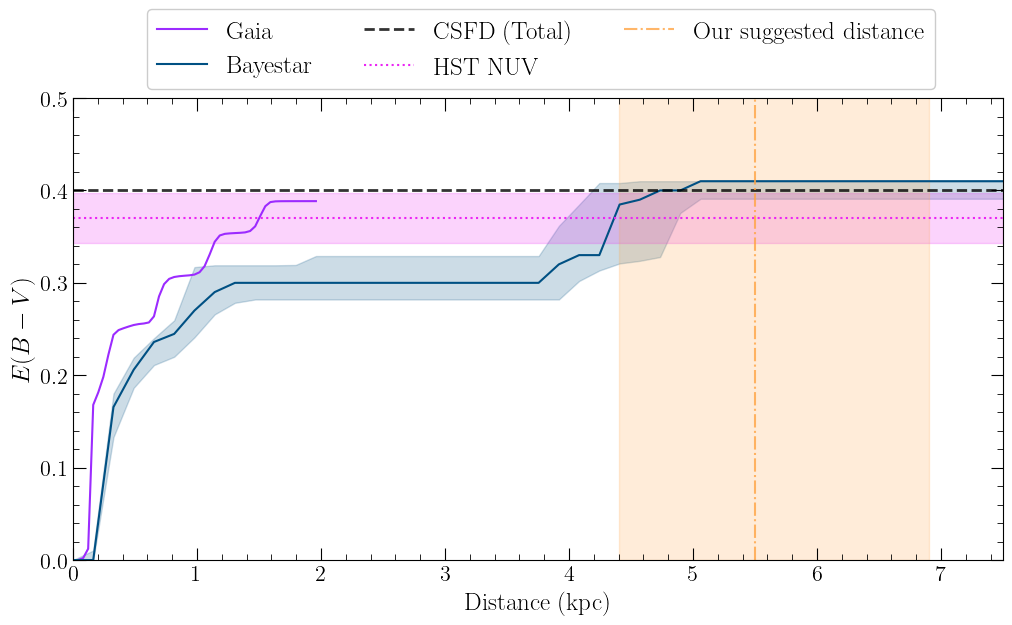
Figure 4: Estimates of $E(B\!-\!V)$ for distances between $0$–$7.5$ kpc along the line of sight to J1727. The 3D Galactic dust maps include Bayestar (blue line; Green et al., 2019) and Gaia (purple line; Edenhofer et al., 2024). We also use an update of the 2D “SFD” dust map (Schlegel et al., 1998) to remove extragalactic contamination that is referred to as the “corrected SFD” (CSFD; grey dashed line; Chiang, 2023). While Green et al. (2019) and Edenhofer et al. (2024) have significant caveats, a comparison between the two clearly shows a more rapid climb in $E(B\!-\!V)$ at closer distances for the Gaia-based map. To investigate the $E(B\!-\!V)$ values that can be reached at $\sim 5$ kpc, we use CSFD, which only reports the total value for $E(B\!-\!V)$ along the line of sight, and therefore serves as a good estimate of the maximum $E(B\!-\!V)$ in the direction of J1727 at high distances. From this we derive a maximum $E(B\!-\!V)\approx 0.4$. Despite disagreement between Bayestar and Gaia in how gas is distributed along the line of sight, both appear to accumulate to roughly this maximum value. Lastly, our estimate of $E(B\!-\!V)$ (pink dotted line) is derived from our near-UV observations. We use this estimate to conclude that values of $E(B\!-\!V)\gg 0.4$ may not be reliable, and suggest a distance to J1727 of $5.5^{+1.4}_{-1.1}$ kpc, which is included for reference (orange dot-dash line).

We note that MS24b calculate a best estimate of the distance to J1727 by assuming equal weights for all methods. Given the unlikely applicability of method 1, and the implausibility of the $E(B\!-\!V)$ values obtained with methods 2 and 3, we suggest using an updated version of method 4.

The reported value for $N_{\rm{H}}$ (Draghis et al., 2023) has been estimated using the tbabs X-ray absorption model and Wilms et al. (2000) abundances of elements. Therefore, the correlation reported by Zhu et al. (2017) becomes a more appropriate choice for estimating extinction than Güver & Özel (2009). Assuming $R_{V}=3.1$ and using equation 11 from Zhu et al. (2017), we estimate $E(B\!-\!V)=0.36\pm 0.11$ along the line of sight to J1727. This is in remarkable agreement with our findings based on near-UV data.

Resampling parameters $10^{5}$ times using Monte Carlo techniques, and using Equation 1 with the MS24b values for $M_{r}$ and $m_{r}$, our estimate of $E(B\!-\!V)$ from $N_{\rm{H}}$ gives a median distance of $5.5^{+1.6}_{-1.3}$ kpc, as compared to a value of $5.5^{+1.4}_{-1.1}$ kpc from our more precise near-UV-derived value. These distance estimates correspond to a GP elevation of $z\approx 1.0^{+0.3}_{-0.2}$ kpc, and a high likelihood that the H i density near J1727 will be well below the level required for H i absorption to be detectable. We collate these distances alongside other estimates in Table 2.

Reference	Method	Reported Distance (kpc)
Abdulghani et al. (2024)	Eddington luminosity fraction	$1.52^{+0.85}_{-0.61}$
Mata Sánchez et al. (2024)	Interstellar Ca ii doublet equivalent width ratio	$3.2\pm 0.6$
Mata Sánchez et al. (2025)	$E(B\!-\!V)$ from interstellar K i 7699 Å  equivalent width	$3.2\pm 1.3$
Mata Sánchez et al. (2025)	$E(B\!-\!V)$ from diffuse interstellar band 8621 Å  equivalent width	$3.5\pm 1.4$
Mata Sánchez et al. (2025)	$E(B\!-\!V)$ from $N_{\rm{H}}$ per Güver & Özel (2009)	$4.8\pm 1.4$
This work	H i absorption kinematic distance	$3.6\pm 0.3\,({stat})\pm 2.3\,({sys})$
This work	$E(B\!-\!V)$ from $N_{\rm{H}}$ per Zhu et al. (2017)	$5.5^{+1.6}_{-1.3}$
This work	$\boldsymbol{E(B\!-\!V)}$ from HST/STIS near-UV observations	$\mathbf{5.5^{+1.4}_{-1.1}}$

Table 2: A comparison of J1727 distance estimates arising from different methods. The ELF-derived distance is likely underestimated (Abdulghani et al., 2024). Where MS24a estimates have been updated since, we use the MS24b values. These both report mean values and are further discussed in Sec. 4.2. The Ca ii method is unlikely to meet the condition that the J1727 is less than a few kpc away from the GP as shown in Sections 4.1.2 and 4.3. The equivalent widths at 7699 Å  and 8621 Å  are both derived using relations from scattered data and infer values of $E(B\!-\!V)$ that are high enough to be unlikely. MS24a acquires an estimate of $N_{\rm{H}}$ from X-ray studies of J1727 and uses $\langle N_{\rm{H}}/A_{V}\rangle$ from Güver & Özel (2009) to calculate $E(B\!-\!V)$, which is reused by MS24b to calculate the distance. The H i absorption kinematic distance derived in this work is a lower bound on the distance as there could be additional distance between the furthest observed H i cloud and J1727. This estimate accounts for the impact of Galactic longitude on kinematic distance methodologies in the form of additional systematic uncertainty. We use the more recent results of Zhu et al. (2017) to implement a larger value of $\langle N_{\rm{H}}/A_{V}\rangle$ and recalculate the distance implied by $N_{\rm{H}}$. Lastly, we use near-UV observations to constrain $E(B\!-\!V)$ and subsequently the distance shown in bold as our preferred estimate. The distance estimates from this work are median values with $1\sigma$ uncertainties.

4.4 Distance implications

Wood et al. (2024) resolved a jet of size $\sim\!110(d/2.7\,\rm{kpc})/\rm{sin}\,\mathit{i}$ AU at 8.4 GHz, where $d$ is the distance and $i$ is the jet axis inclination angle. Our suggested distance of $5.5^{+1.4}_{-1.1}$ kpc suggests a jet size $>200$ AU regardless of the inclination angle used.

Liu et al. (2024) found that in the hard state at the beginning of the J1727 outburst, the broadband X-ray flux was $\sim 3\times 10^{-7}\ \rm{erg\ cm^{-2}\ s^{-1}}$. At a distance of $5.5^{+1.4}_{-1.1}$ kpc, this would correspond to a luminosity of $\sim 1.1\times 10^{39}\ \rm{erg\ s^{-1}}$, which is equivalent to $L_{\rm{Edd}}$ for an $8.6\,\rm{M}_{\odot}$ BH accreting hydrogen. While these luminosities are unusually high for the pure hard state, it is not impossible (Tetarenko et al., 2016).

The inferred natal kick velocity of J1727 is also impacted by an increase in the estimated distance. MS24b used their estimated distance of $3.4\pm 0.3$ kpc, along with the proper motion of J1727, to derive a median and 68% confidence level in the potential natal kick velocity of $v_{\rm{kick}}=210^{+40}_{-50}$ km s^-1. Our new distance revises this to $v_{\rm{kick}}=190\pm 30$ km s^-1(Atri et al., 2019).

5 Conclusions

Using H i absorption data from MeerKAT observations of the outburst of Swift J1727.8$-$1613, we determine a maximum absorption velocity of $24.8\pm 2.8$ km s^-1. The higher-velocity absorption seen towards the extragalactic reference source PKS J1733$-$1304 allows us to use the near kinematic distance as a lower bound of $3.6\pm 0.3\,({stat})\pm 2.3\,({sys})$ kpc, accounting for the systematic uncertainty due to the low Galactic longitude of the source. Its high Galactic latitude likely implies that we run out of H i clouds along the line of sight, suggesting that the true distance could be significantly greater.

We therefore make use of a near-UV spectrum of Swift J1727.8$-$1613 as observed by the Space Telescope Imaging Spectrograph aboard the Hubble Space Telescope. This allows us to estimate the colour excess or reddening as $E(B\!-\!V)=0.37\pm 0.01\,({stat})\pm 0.025\,({sys})$. This is significantly lower than previous constraints on $E(B\!-\!V)$ from Mata Sánchez et al. (2024, 2025), but is in good agreement the maximum value derived from Galactic dust maps along this line of sight, and suggests that previous works underestimated the distance.

Using $E(B\!-\!V)$ to determine the $r$-band extinction and combining this with donor star $r$-band magnitudes measured by Mata Sánchez et al. (2025), we present $5.5^{+1.4}_{-1.1}$ kpc as the resulting and likely distance to Swift J1727.8$-$1613. This places the system much farther away than previously thought and implies a natal kick velocity of $v_{\rm{kick}}=190\pm 30$ km s^-1.

References

- Abdulghani et al. (2024) Abdulghani, Y., Lohfink, A. M., & Chauhan, J. 2024, MNRAS, 530, 424, doi: 10.1093/mnras/stae767
- Abril-Pla et al. (2023) Abril-Pla, O., Andreani, V., Carroll, C., et al. 2023, PeerJ Computer Science, 9, e1516, doi: 10.7717/peerj-cs.1516
- Arnason et al. (2021) Arnason, R. M., Papei, H., Barmby, P., Bahramian, A., & Gorski, M. D. 2021, MNRAS, 502, 5455, doi: 10.1093/mnras/stab345
- Astropy Collaboration et al. (2022) Astropy Collaboration, Price-Whelan, A. M., Lim, P. L., et al. 2022, ApJ, 935, 167, doi: 10.3847/1538-4357/ac7c74
- Atri et al. (2019) Atri, P., Miller-Jones, J. C. A., Bahramian, A., et al. 2019, MNRAS, 489, 3116, doi: 10.1093/mnras/stz2335
- Atri et al. (2020) —. 2020, MNRAS, 493, L81, doi: 10.1093/mnrasl/slaa010
- Beardmore et al. (2016) Beardmore, A. P., Willingale, R., Kuulkers, E., et al. 2016, MNRAS, 462, 1847, doi: 10.1093/mnras/stw1753
- Bright et al. (2023) Bright, J., Farah, W., Fender, R., et al. 2023, The Astronomer’s Telegram, 16228, 1. https://www.astronomerstelegram.org/?read=16228
- Camilo (2018) Camilo, F. 2018, Nature Astronomy, 2, 594, doi: 10.1038/s41550-018-0516-y
- Cardelli et al. (1989) Cardelli, J. A., Clayton, G. C., & Mathis, J. S. 1989, ApJ, 345, 245, doi: 10.1086/167900
- CASA Team et al. (2022) CASA Team, Bean, B., Bhatnagar, S., et al. 2022, PASP, 134, 114501, doi: 10.1088/1538-3873/ac9642
- Castro Segura et al. (2020) Castro Segura, N., Altamirano, D., Buisson, D., et al. 2020, Outflow Legacy Accretion Survey: unveiling the wind driving mechanism in BHXRBs, HST Proposal. Cycle 28, ID. #16489
- Castro-Tirado et al. (2023) Castro-Tirado, A. J., Sanchez-Ramirez, R., Caballero-Garcia, M. D., et al. 2023, The Astronomer’s Telegram, 16208, 1. https://www.astronomerstelegram.org/?read=16208
- Charles et al. (2019) Charles, P., Matthews, J. H., Buckley, D. A. H., et al. 2019, MNRAS, 489, L47, doi: 10.1093/mnrasl/slz120
- Chauhan et al. (2019) Chauhan, J., Miller-Jones, J. C. A., Anderson, G. E., et al. 2019, MNRAS, 488, L129, doi: 10.1093/mnrasl/slz113
- Chauhan et al. (2021) Chauhan, J., Miller-Jones, J. C. A., Raja, W., et al. 2021, MNRAS, 501, L60, doi: 10.1093/mnrasl/slaa195
- Chiang (2023) Chiang, Y.-K. 2023, ApJ, 958, 118, doi: 10.3847/1538-4357/acf4a1
- Comrie et al. (2021) Comrie, A., Wang, K.-S., Hsu, S.-C., et al. 2021, CARTA: The Cube Analysis and Rendering Tool for Astronomy, 2.0.0, Zenodo, doi: 10.5281/zenodo.3377984
- Dhawan et al. (2007) Dhawan, V., Mirabel, I. F., Ribó, M., & Rodrigues, I. 2007, ApJ, 668, 430, doi: 10.1086/520111
- Dickey (1983) Dickey, J. M. 1983, ApJ, 273, L71, doi: 10.1086/184132
- Draghis et al. (2023) Draghis, P. A., Miller, J. M., Homan, J., et al. 2023, The Astronomer’s Telegram, 16219, 1
- Dubus et al. (2001) Dubus, G., Kim, R. S. J., Menou, K., Szkody, P., & Bowen, D. V. 2001, ApJ, 553, 307, doi: 10.1086/320648
- Edenhofer et al. (2024) Edenhofer, G., Zucker, C., Frank, P., et al. 2024, A&A, 685, A82, doi: 10.1051/0004-6361/202347628
- Fender et al. (2016) Fender, R., Woudt, P. A., Corbel, S., et al. 2016, in MeerKAT Science: On the Pathway to the SKA, 13, doi: 10.22323/1.277.0013
- Fitzpatrick (2004) Fitzpatrick, E. L. 2004, in Astronomical Society of the Pacific Conference Series, Vol. 309, Astrophysics of Dust, ed. A. N. Witt, G. C. Clayton, & B. T. Draine, 33, doi: 10.48550/arXiv.astro-ph/0401344
- Gandhi et al. (2019) Gandhi, P., Rao, A., Johnson, M. A. C., Paice, J. A., & Maccarone, T. J. 2019, MNRAS, 485, 2642, doi: 10.1093/mnras/stz438
- Green (2018) Green, G. 2018, The Journal of Open Source Software, 3, 695, doi: 10.21105/joss.00695
- Green et al. (2019) Green, G. M., Schlafly, E., Zucker, C., Speagle, J. S., & Finkbeiner, D. 2019, ApJ, 887, 93, doi: 10.3847/1538-4357/ab5362
- Güver & Özel (2009) Güver, T., & Özel, F. 2009, MNRAS, 400, 2050, doi: 10.1111/j.1365-2966.2009.15598.x
- Hack et al. (2018) Hack, W., Dencheva, N., Sontag, C., Sosey, M., & Droettboom, M. 2018, STIS Python User Tools. https://stistools.readthedocs.io/en/latest/index.html
- Harris et al. (2020) Harris, C. R., Millman, K. J., van der Walt, S. J., et al. 2020, Nature, 585, 357, doi: 10.1038/s41586-020-2649-2
- Heinz et al. (2015) Heinz, S., Burton, M., Braiding, C., et al. 2015, ApJ, 806, 265, doi: 10.1088/0004-637X/806/2/265
- Hunter et al. (2024) Hunter, G. H., Sormani, M. C., Beckmann, J. P., et al. 2024, A&A, 692, A216, doi: 10.1051/0004-6361/202450000
- Hunter (2007) Hunter, J. D. 2007, Computing in Science & Engineering, 9, 90, doi: 10.1109/MCSE.2007.55
- Jonker & Nelemans (2004) Jonker, P. G., & Nelemans, G. 2004, MNRAS, 354, 355, doi: 10.1111/j.1365-2966.2004.08193.x
- Kalberla & Kerp (2009) Kalberla, P. M. W., & Kerp, J. 2009, ARA&A, 47, 27, doi: 10.1146/annurev-astro-082708-101823
- Kalemci et al. (2013) Kalemci, E., Dinçer, T., Tomsick, J. A., et al. 2013, ApJ, 779, 95, doi: 10.1088/0004-637X/779/2/95
- Kluyver et al. (2016) Kluyver, T., Ragan-Kelley, B., Pérez, F., et al. 2016, in IOS Press, 87–90, doi: 10.3233/978-1-61499-649-1-87
- Lamer et al. (2021) Lamer, G., Schwope, A. D., Predehl, P., et al. 2021, A&A, 647, A7, doi: 10.1051/0004-6361/202039757
- Liu et al. (2024) Liu, H.-X., Xu, Y.-J., Zhang, S.-N., et al. 2024, arXiv e-prints, arXiv:2406.03834, doi: 10.48550/arXiv.2406.03834
- Lockman et al. (2007) Lockman, F. J., Blundell, K. M., & Goss, W. M. 2007, MNRAS, 381, 881, doi: 10.1111/j.1365-2966.2007.12170.x
- Mata Sánchez et al. (2024) Mata Sánchez, D., Muñoz-Darias, T., Armas Padilla, M., Casares, J., & Torres, M. A. P. 2024, A&A, 682, L1, doi: 10.1051/0004-6361/202348754
- Mata Sánchez et al. (2025) Mata Sánchez, D., Torres, M. A. P., Casares, J., et al. 2025, A&A, 693, A129, doi: 10.1051/0004-6361/202451960
- Megier et al. (2009) Megier, A., Strobel, A., Galazutdinov, G. A., & Krełowski, J. 2009, A&A, 507, 833, doi: 10.1051/0004-6361/20079144
- Miller-Jones et al. (2023a) Miller-Jones, J. C. A., Bahramian, A., Altamirano, D., et al. 2023a, The Astronomer’s Telegram, 16271, 1. https://www.astronomerstelegram.org/?read=16271
- Miller-Jones et al. (2009) Miller-Jones, J. C. A., Jonker, P. G., Dhawan, V., et al. 2009, ApJ, 706, L230, doi: 10.1088/0004-637X/706/2/L230
- Miller-Jones et al. (2023b) Miller-Jones, J. C. A., Sivakoff, G. R., Bahramian, A., & Russell, T. D. 2023b, The Astronomer’s Telegram, 16211, 1. https://www.astronomerstelegram.org/?read=16211
- Miller-Jones et al. (2021) Miller-Jones, J. C. A., Bahramian, A., Orosz, J. A., et al. 2021, Science, 371, 1046, doi: 10.1126/science.abb3363
- Munari & Zwitter (1997) Munari, U., & Zwitter, T. 1997, A&A, 318, 269
- Negoro et al. (2023) Negoro, H., Serino, M., Nakajima, M., et al. 2023, The Astronomer’s Telegram, 16205, 1. https://www.astronomerstelegram.org/?read=16205
- O’Connor et al. (2023) O’Connor, B., Hare, J., Younes, G., et al. 2023, The Astronomer’s Telegram, 16207, 1
- Reid (2022) Reid, M. J. 2022, AJ, 164, 133, doi: 10.3847/1538-3881/ac80bb
- Reid et al. (2011) Reid, M. J., McClintock, J. E., Narayan, R., et al. 2011, ApJ, 742, 83, doi: 10.1088/0004-637X/742/2/83
- Reid & Miller-Jones (2023) Reid, M. J., & Miller-Jones, J. C. A. 2023, ApJ, 959, 85, doi: 10.3847/1538-4357/acfe0c
- Reid et al. (2014) Reid, M. J., Menten, K. M., Brunthaler, A., et al. 2014, ApJ, 783, 130, doi: 10.1088/0004-637X/783/2/130
- Reid et al. (2019) —. 2019, ApJ, 885, 131, doi: 10.3847/1538-4357/ab4a11
- Rybarczyk et al. (2024) Rybarczyk, D. R., Wenger, T. V., & Stanimirović, S. 2024, ApJ, 975, 167, doi: 10.3847/1538-4357/ad79f7
- Sault et al. (1995) Sault, R. J., Teuben, P. J., & Wright, M. C. H. 1995, in Astronomical Society of the Pacific Conference Series, Vol. 77, Astronomical Data Analysis Software and Systems IV, ed. R. A. Shaw, H. E. Payne, & J. J. E. Hayes, 433, doi: 10.48550/arXiv.astro-ph/0612759
- Savage & Mathis (1979) Savage, B. D., & Mathis, J. S. 1979, ARA&A, 17, 73, doi: 10.1146/annurev.aa.17.090179.000445
- Schlafly & Finkbeiner (2011) Schlafly, E. F., & Finkbeiner, D. P. 2011, ApJ, 737, 103, doi: 10.1088/0004-637X/737/2/103
- Schlegel et al. (1998) Schlegel, D. J., Finkbeiner, D. P., & Davis, M. 1998, ApJ, 500, 525, doi: 10.1086/305772
- Tetarenko et al. (2016) Tetarenko, B. E., Sivakoff, G. R., Heinke, C. O., & Gladstone, J. C. 2016, ApJS, 222, 15, doi: 10.3847/0067-0049/222/2/15
- Vahdat Motlagh et al. (2019) Vahdat Motlagh, A., Kalemci, E., & Maccarone, T. J. 2019, MNRAS, 485, 2744, doi: 10.1093/mnras/stz569
- Virtanen et al. (2020) Virtanen, P., Gommers, R., Oliphant, T. E., et al. 2020, Nature Methods, 17, 261, doi: 10.1038/s41592-019-0686-2
- Wallerstein et al. (2007) Wallerstein, G., Sandstrom, K., & Gredel, R. 2007, PASP, 119, 1268, doi: 10.1086/521835
- Wenger (2018) Wenger, T. V. 2018, tvwenger/kd v1.0, v1.0, Zenodo, doi: 10.5281/zenodo.1166001
- Wenger et al. (2018) Wenger, T. V., Balser, D. S., Anderson, L. D., & Bania, T. M. 2018, ApJ, 856, 52, doi: 10.3847/1538-4357/aaaec8
- Wilms et al. (2000) Wilms, J., Allen, A., & McCray, R. 2000, ApJ, 542, 914, doi: 10.1086/317016
- Wood et al. (2024) Wood, C. M., Miller-Jones, J. C. A., Bahramian, A., et al. 2024, ApJ, 971, L9, doi: 10.3847/2041-8213/ad6572
- Woodgate et al. (1998) Woodgate, B. E., Kimble, R. A., Bowers, C. W., et al. 1998, PASP, 110, 1183, doi: 10.1086/316243
- Zhu et al. (2017) Zhu, H., Tian, W., Li, A., & Zhang, M. 2017, MNRAS, 471, 3494, doi: 10.1093/mnras/stx1580