FEMBA: Efficient and Scalable EEG Analysis with a
Bidirectional Mamba Foundation Model

Abstract

Accurate and efficient electroencephalography (EEG) analysis is essential for detecting seizures and artifacts in long-term monitoring, with applications spanning hospital diagnostics to wearable health devices. Robust EEG analytics have the potential to greatly improve patient care. However, traditional deep learning models, especially Transformer-based architectures, are hindered by their quadratic time and memory complexity, making them less suitable for resource-constrained environments. To address these challenges, we present FEMBA (Foundational EEG Mamba + Bidirectional Architecture), a novel self-supervised framework that establishes new efficiency benchmarks for EEG analysis through bidirectional state-space modeling. Unlike Transformer-based models, which incur quadratic time and memory complexity, FEMBA scales linearly with sequence length, enabling more scalable and efficient processing of extended EEG recordings. Trained on over 21,000 hours of unlabeled EEG and fine-tuned on three downstream tasks, FEMBA achieves competitive performance in comparison with transformer models, with significantly lower computational cost. Specifically, it reaches 81.82% balanced accuracy (0.8921 AUROC) on TUAB and 0.949 AUROC on TUAR, while a tiny 7.8M-parameter variant demonstrates viability for resource-constrained devices. These results pave the way for scalable, general-purpose EEG analytics in both clinical and highlight FEMBA as a promising candidate for wearable applications.
Clinical relevance— By reducing model size and computational overhead, FEMBA enables continuous on-device EEG monitoring for tasks like seizure detection and artifact reduction, promising improved patient care through timely and cost-effective neuro-monitoring solutions.

I Introduction

The emergence of foundation models has profoundly impacted artificial intelligence, bringing forward a shift toward generalizable, large-scale pre-training. These models, trained via self-supervised learning (SSL) on heterogeneous datasets, derive their effectiveness from hierarchical feature extraction that can span diverse tasks [1]. While their success in language (e.g., BERT [2]) and vision (e.g., CLIP [3]) is well-documented, their potential in biomedical signal processing—particularly for Electroencephalography (EEG) —remains relatively underexplored.

EEG is a challenging modality due to its pseudo-random, non-stationary waveforms, susceptibility to artifacts [4], and substantial intra- and inter-subject variability. These factors demand models that balance robustness with interpretability. Wearable EEG devices play a crucial role in enabling continuous brain monitoring in real-world settings, offering new opportunities for brain-computer interfaces [5], healthcare and cognitive research [6]. Although recent efforts have used convolutional architectures [7] and attention-based mechanisms [8] for EEG, real-world constraints complicate their deployment. Wearable devices and continuous monitoring systems impose strict limits on memory and latency [9], making even moderately sized Transformers impractical. As a result, there is a strong, important, unmet need for architectures that can combine expressive power with computational efficiency. Given these constraints, we propose harnessing State Space Models (SSMs). Specifically, we build upon the Mamba linear SSM, a scalable approach tailored for large-scale EEG, to mitigate the memory and latency bottlenecks associated with Transformer models while maintaining high performance and interpretability.

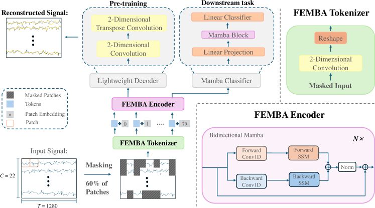
Figure 1: Overview of the proposed FEMBA (Foundational EEG Mamba + Bidirectional Architecture) pipeline. The input EEG signal (with channels $C$ and length $T$) is first tokenized via a 2D convolution and flattening layer. Random masking is then applied to a subset of the patches for self-supervised learning. The masked tokens pass through the FEMBA encoder, which stacks multiple Bidirectional Mamba blocks to capture forward and backward dependencies. Finally, a lightweight decoder (for reconstruction) or a classification head (for downstream tasks) reconstructs or classifies the signals, respectively.

From Transformers to Mamba

Transformer-based models have demonstrated strong performance in capturing long-range dependencies in EEG [8, 10]. Current EEG foundation models (e.g., BENDR, EEGFormer, LaBraM, Neuro-GPT) predominantly rely on attention mechanisms and may not provide the efficiency demanded by edge-computing environments. However, their $\mathcal{O}(N^{2})$ complexity in computation and memory as a function of sequence length N can become a bottleneck for continuous or extended EEG recordings, especially on resource-constrained devices. In contrast, Mamba [11], which is based on a state-space framework, helps address these challenges by reformulating sequence modeling as a latent differential system. This approach offers linear scaling (as a function of sequence length) without substantially compromising temporal resolution. Bidirectional extensions [12] further enable retrospective analysis, which may be essential for detecting ephemeral biomarkers (e.g., interictal spikes).

To investigate computationally efficient architectures such alternatives, we introduce FEMBA (Foundational EEG Mamba + Bidirectional Architecture), which leverages state-space principles for large-scale EEG modeling. FEMBA is designed to address three key limitations of prior work: (1) quadratic scaling in attention-based models, (2) limited pre-training scope for capturing neurophysiological diversity, and (3) difficulties in adapting to low-resource settings. By pre-training on 21,000 hours of unlabeled EEG from 5,000 subjects, FEMBA aims to learn representations that generalize across a range of pathologies, while retaining the potential for deployment on wearable hardware, as demonstrated by the promising performance of our Tiny FEMBA model.

Our contributions are the following:

• A Novel Architectural Paradigm: We integrate a bidirectional state-space approach with SSL to demonstrate that linear-time architectures can match—or in some cases surpass—Transformer-based models on established EEG benchmarks (TUAB, TUAR, TUSL). This result suggests that attention-based solutions may not always be indispensable for effective EEG modeling.

• Large-Scale Pre-training on EEG: We conduct pre-training on a terabyte-scale unlabeled EEG dataset (over 21,000 hours of data from more than 5,000 participants) that spans multiple studies. Using random masking for self-supervised reconstruction, FEMBA acquires robust, general representations suitable for diverse downstream tasks without extensive labeled data.

• Efficient state-of-the-art (SOTA) performance We have developed FEMBA in four sizes of model parameters: Tiny (7.8M), Base (47.7M), Large (77.8M), and Huge (389M). The Huge model achieves a mere 0.7% decrease in accuracy compared to the SOTA on TUAB while being $3.5\times$ more computationally efficient and $1.5\times$ more memory efficient. On TUAR, FEMBA sets a new SOTA benchmark, with the Tiny model beating previous SOTA with over $27\times$ computational decrease and over $2\times$ better memory efficiency compared to the previous SOTA. These results highlight FEMBA’s versatility for high-performance applications and resource-restrictive scenarios.

By emphasizing both effectiveness and efficiency, FEMBA provides a step toward accessible, low-cost analytics in healthcare contexts. The remainder of this paper details the methodology and experiments, highlighting how state-space-based approaches can offer a compelling alternative to attention-driven architectures in EEG analysis.

II Background

This section provides an overview of the Temple University Hospital EEG (TUEG) Corpus and its labeled subsets, then reviews recent advances in EEG foundation models. We focus on the computational challenges faced by Transformer-based approaches, discuss the motivation for SSMs, and examine Mamba-based solutions. Finally, we introduce how our proposed FEMBA architecture builds upon these insights.

II-A Temple University Hospital EEG (TUEG)

The TUEG Corpus [13], is one of the largest publicly available clinical EEG repositories. It contains over $26{,}000$ EEG recordings drawn from more than $14{,}000$ patients, spanning pediatric to geriatric populations and encompassing a variety of neurological conditions. In total, TUEG covers approximately $21{,}000$ hours of EEG data. Such diversity in demographics and pathologies provides a robust environment for learning general EEG representations.

II-B Key Labeled Subsets: TUAB, TUAR, and TUSL

The TUEG dataset offers subsets of labeled datasets, such as the Temple University Hospital Abnormal EEG (TUAB), Artifact (TUAR) and Slowing (TUSL) Corpus [13]. TUAB offers annotated recordings labeled as normal or abnormal. TUAB has $2,329$ subjects and relatively balanced classes and TUAB serves as a strong benchmark for clinical diagnostics. The TUAR dataset contains annotations for various artifacts (e.g., eye blinks, muscle artifacts) in single-channel or multi-channel settings and has $213$ subjects. While in TUSL, the focus shifts to detecting and classifying slowing events, seizures, complex background, and normal EEG. This 4-class classification task (slowing, seizure, complex, normal) consists of $1000$ subjects. Table I summarizes these three labeled subsets used in our experiments.

TABLE I: Summary of Datasets Used

Dataset	# Subjects	Task
TUEG	$14{,}987$	Pre-training
TUAB	$2{,}329$	Abnormal vs. Normal
TUAR	213	Artifact Detection
TUSL	$1{,}000$	Slowing Events

II-C Related works

Foundation Models in EEG

Foundation models have gained significant traction in NLP (e.g., DeepSeek [14]) and computer vision (e.g., Molmo [15]), motivating interest in their application to EEG. However, these models are typically tailored for structured data such as text or images, raising challenges when dealing with the temporal complexity and biological variability of EEG signals [16]. Early EEG-focused foundation models like BENDR [17] employed contrastive learning yet faced scalability issues. Neuro-GPT [18] introduced autoregressive masking and reported gains in motor imagery classification, while LaBraM [10] and EEGFormer [8] refined masked modeling methods across multiple datasets, achieving balanced accuracies above 80% on abnormal EEG detection. Despite these advancements, most prior approaches rely on Transformer architectures with $\mathcal{O}(N^{2})$ complexity as a function of the sequence length, limiting their viability for continuous or large-scale EEG monitoring.

From Traditional Methods to State Space Models

Conventional EEG analysis often used machine learning algorithms such as Support Vector Machines (SVMs) and Linear Discriminant Analysis (LDA), complemented by smaller deep networks like EEGNet [19] and DeepConvNet [20]. While these approaches offered interpretability and efficiency for relatively constrained tasks, they required extensive feature engineering and did not always generalize well to diverse patient populations. Transformer-based methods [10, 8, 18, 17] later tackled the challenge of capturing long-range dependencies, though their substantial computational and memory demands may hinder real-world deployment.

SSMs have gained interest for time-series analysis as they evolve a hidden state over time according to a simple linear dynamical system. In continuous form

$$\mathbf{h}^{\prime}(t)=A\,\mathbf{h}(t)+B\,\mathbf{x}(t),\quad\mathbf{y}(t)=C\,\mathbf{h}(t),$$

where $\mathbf{h}(t)$ is the hidden state, $\mathbf{x}(t)$ is the input, $\mathbf{y}(t)$ is the output, and $\{A,B,C\}$ are system matrices governing state evolution and output generation. Although these equations describe a continuous process, many implementations rely on discrete versions for efficient training in deep learning frameworks.

Wearable and Edge Constraints

Limited battery life, on-board memory, and compute resources characterize many real-world EEG applications, especially wearable devices [21]. Applications like continuous epilepsy detection add real-time considerations and demand low false-alarm rates [4]. The quadratic scaling of transformer-based methods often proves impractical under these constraints. In contrast, architectures based on state-space principles—owing to linear time and memory complexity—can better meet edge-computing requirements.

Mamba-Based Approaches for EEG

A notable example of such SSM is Mamba [11], which applies a Zero-Order Hold (ZOH) scheme [22] to discretize the SSM. Under a sampling interval $\Delta$, the continuous matrices $A,B$ map to discrete counterparts $A_{d}$ and $B_{d}$. Mamba further integrates a selective gating mechanism to modulate the hidden state update in a data-dependent manner. As a result, it achieves linear complexity in sequence length, contrasting with the $\mathcal{O}(N^{2})$ complexity of transformers. Bi-Mamba+ [12] extends Mamba by processing the input sequence in forward and backward directions, subsequently merging the two representations (e.g., via summation or gating). Recent work has begun to explore Mamba’s potential in EEG analysis. Mentality [23] employed Mamba with a masked reconstruction scheme on TUSZ v2.0.1, improving seizure detection area under the ROC curve (AUROC) from 0.64 to 0.72. EEGMamba [24] adopted a multi-task strategy by integrating Spatio-Temporal-Adaptive modules and Mixture-of-Experts heads, achieving above 98% accuracy on the Siena dataset and around 97% on CHB-MIT. Despite these early successes, challenges for Mamba-based models remain—especially regarding robust spatial-channel modeling for varying electrode montages and the need for domain-generalizable representations.

In this work, our FEMBA builds upon Mamba’s efficient state-space design by integrating large-scale self-supervised pre-training with bidirectional state updates, FEMBA aims to deliver strong accuracy on various EEG downstream tasks while maintaining linear scaling (with regards to sequence length) suitable for resource-limited devices.

III Methodology

In this section, we describe the proposed Foundational EEG Mamba + Bidirectional Architecture (FEMBA) and its training procedures. Next, we outline our self-supervised pre-training scheme and finally, we explain our fine-tuning strategy, including two alternative classifier architectures and multiple downstream tasks (abnormal EEG detection, artifact recognition, and slowing event classification).

III-A Foundational EEG Mamba + Bidirectional Architecture (FEMBA)

Our proposed FEMBA architecture is designed in four model sizes: Tiny, Base, Large, and Huge, with parameter sizes ranging from 7.8 million (Tiny) to 386 million (Huge), aligning with model sizes commonly explored in the literature [10, 8]. The primary distinction across these variants lies in the number of Bi-Mamba blocks and the embedding dimension, which is controlled by the 2D Convolution in the Tokenizer, as illustrated in Fig 1. Specifically, the embedding dimensions for these configurations are as follows: the Tiny model uses two blocks and an embedding size of 35 ($(2,35)$); the Base model employs a configuration of $(12,35)$; the Large model adopts $(4,79)$; and the Huge model features $(20,79)$. Notably, the hidden state size across all configurations remains fixed at 80.

Furthermore, a residual connection is incorporated within the Bi-Mamba block to facilitate the smooth propagation of gradients during training. A detailed representation of the entire FEMBA architecture can be found in Fig 1.

During training, we utilize a layer-wise learning rate decay [25] with a fixed decay factor of $0.75$, progressively reducing the learning rate from the deeper blocks to the earlier ones

III-B Self-Supervised Pre-training

We pre-train FEMBA on the TUEG dataset, as detailed in Section II-A. To prevent data leakage between pre-training and downstream tasks, we use a version of TUEG where subjects present in TUSL, TUAR, or TUAB have been filtered out. During pre-training, we adopt a self-supervised masked training strategy designed to enable FEMBA to learn robust, general-purpose representations of EEG signals. This involves randomly masking a subset (60%) of the input patches and training the model to reconstruct the missing patches, thereby compelling the encoder to capture meaningful spatiotemporal structures within the EEG data.

Signal Normalization and Patch Embedding.

We begin by representing each raw EEG recording as a tensor $x\in\mathbb{R}^{C\times T}$, where $C$ is the number of channels and $T$ is the temporal length (in samples). To reduce the influence of outliers, we apply quartile-based normalization [26], scaling each channel by its interquartile range (IQR):

$$x_{\text{norm}}=\frac{x-q_{\text{lower}}}{(q_{\text{upper}}-q_{\text{lower}})+1\times 10^{-8}}.$$

We then segment $x_{\text{norm}}$ into bi-dimensional patches of size $p\times q$ (e.g., $4$ channels $\times$ $32$ samples). A 2D convolution projects these patches into an embedding space $\mathbf{X}_{\text{embed}}\in\mathbb{R}^{d\times C^{\prime}\times T^{\prime}}$, followed by learnable positional embeddings to maintain ordering across patch tokens.

Random Masking and Encoder.

Next, we apply random masking to $60\%$ of the embedded patches, setting their representations to zero. This relatively high masking ratio ensures that the model must rely on contextual cues from unmasked segments to infer the missing patches. The masked embeddings, $\mathbf{X}_{\text{masked}}$, are then fed into the FEMBA encoder.

Decoder and Smooth L1 Reconstruction Loss.

A lightweight decoder of two convolutional layers and a final linear projection attempts to reconstruct the original patches from the encoder outputs. We compute a Smooth L1 loss [27] only over the masked patches:

$$\text{SmoothL1}(\hat{x},x)=\begin{cases}0.5\,(x-\hat{x})^{2},&\text{if }|x-\hat{x}|<\beta,\\ |x-\hat{x}|-0.5,&\text{otherwise},\end{cases}$$

$$\text{masked\_loss}=\frac{1}{|\mathcal{M}|}\sum_{i\in\mathcal{M}}\text{SmoothL1}(\hat{x}_{i},x_{i}),$$

where $\mathcal{M}$ is the set of masked patch indices.

III-C Fine-Tuning

III-C1 Classifier Architectures.

Following pre-training, the decoder is discarded and the Bi-Mamba encoder is repurposed as a feature extractor for downstream tasks. Two classification heads are explored:

1. Linear Classifier: A small stack of fully connected layers (with GELU activations) outputs class probabilities. This design has a low parameter footprint ($\sim 0.5$ M).

2. Mamba-Enhanced Classifier: We add one more Mamba block before the final linear layer, enabling additional temporal modeling. This often improves accuracy in tasks with complex temporal dependencies but adds a slight increase in parameters (up to $0.7$ M).

III-C2 Downstream tasks

We assess FEMBA on three downstream tasks using the datasets described in Section II-B. For the TUAB dataset this consists of a binary classification (normal vs. abnormal), using the pre-defined train-test split. In TUSL, the task is a four-class classification task (slowing, seizure, complex, normal), Since the TUSL dataset lacks a predefined test split, we adopt an 80/10/10 randomized training/validation/test split. For TUAR we experiment with four versions of a downstream task based on the labeling scheme in in [28], they are described as the following:

• Binary Classification (BC): Label a window as artifact if any of the 13 artifact types is present on any channel; otherwise normal.

• Multilabel Classification (MC): Perform channel-wise artifact detection as a set of independent binary classifications, allowing multiple artifact types per window/channel.

• Multiclass–Multioutput Classification (MMC): Discriminate between 13 artifact types for each channel, thus providing a more granular classification per channel.

• Multiclass Classification (MCC): Restrict to 5 artifact types in a single-label setting, ignoring windows with combinations of artifacts (less than 5% of data). This setting aligns closely with the protocol described by EEGFormer [8].

As the TUAR dataset also lacks a predefined test split, we similarly use an 80/10/10 randomized training/validation/test split.

IV Results

This section demonstrates that FEMBA consistently achieves state-of-the-art (SoA) or near-SoA performance on diverse EEG benchmarks (TUAB, TUAR, and TUSL), while using significantly fewer FLOPs and less memory compared to recent SoA self-supervised Transformer-based methods. We provide quantitative accuracy metrics and efficiency analyses, which underscores FEMBA’s suitability for large-scale clinical or wearable EEG systems. For specific training details we fine-tune all layers (encoder + classifier) end-to-end using the Adam optimizer (initial learning rate of $1\times 10^{-4}$) with cosine decay scheduling. Early stopping is employed based on validation loss to mitigate overfitting.

TABLE II: Performance Comparison on TUAB

Model	Model Size	Bal. Acc. (%)	AUPR	AUROC
Supervised Models
SPaRCNet	0.8M	78.96 $\pm$ 0.18	0.8414 $\pm$ 0.0018	0.8676 $\pm$ 0.0012
ContraWR	1.6M	77.46 $\pm$ 0.41	0.8421 $\pm$ 0.0140	0.8456 $\pm$ 0.0074
CNN-Transformer	3.2M	77.77 $\pm$ 0.22	0.8433 $\pm$ 0.0039	0.8461 $\pm$ 0.0013
FFCL	2.4M	78.48 $\pm$ 0.38	0.8448 $\pm$ 0.0065	0.8569 $\pm$ 0.0051
ST-Transformer	3.2M	79.66 $\pm$ 0.23	0.8521 $\pm$ 0.0026	0.8707 $\pm$ 0.0019
Self-superv. Models
BENDR	0.39M	76.96 $\pm$ 3.98		0.8397 $\pm$ 0.0344
BrainBERT	43.2M	-	0.8460 $\pm$ 0.0030	0.8530 $\pm$ 0.0020
EEGFormer-Small	1.9M	-	0.8620 $\pm$ 0.0050	0.8620 $\pm$ 0.0070
EEGFormer-Base	2.3M	-	0.8670 $\pm$ 0.0020	0.8670 $\pm$ 0.0030
EEGFormer-Large	3.2M	-	0.8720 $\pm$ 0.0010	0.8760 $\pm$ 0.0030
BIOT	3.2M	79.59 $\pm$ 0.57	0.8692 $\pm$ 0.0023	0.8815 $\pm$ 0.0043
EEG2Rep	-	80.52 $\pm$ 2.22		0.8843 $\pm$ 0.0309
LaBraM-Base	5.8M	81.40 $\pm$ 0.19	0.8965 $\pm$ 0.0016	0.9022 $\pm$ 0.0009
LaBraM-Large	46M	82.26 $\pm$ 0.15	0.9130 $\pm$ 0.0005	0.9127 $\pm$ 0.0005
LaBraM-Huge	369M	82.58 $\pm$ 0.11	0.9204 $\pm$ 0.0011	0.9162 $\pm$ 0.0016
FEMBA-Base	47.7M	81.05 $\pm$ 0.14	0.8894 $\pm$0.0050	0.8829 $\pm$ 0.0021
FEMBA-Large	77.8M	81.47 $\pm$ 0.11	0.8992 $\pm$ 0.0007	0.8856 $\pm$ 0.0004
FEMBA-Huge	386M	81.82 $\pm$ 0.16	0.9005 $\pm$ 0.0017	0.8921 $\pm$ 0.0042

TABLE III: Model Comparison of FLOPs, Parameters, and Peak Memory Usage

Model	FLOPs	Parameters	Memory (MB)
EEGFormer-Small	21.06B	1.9M	44.63
EEGFormer-Base	26.20B	2.3M	71.32
EEGFormer-Large	36.46B	3.2M	108.02
LaBraM-Base	4.42B	5.8M	757.38
LaBraM-Large	27.79B	46M	1371.92
LaBraM-Huge	202.17B	369M	2758.42
FEMBA-Tiny	1.31B	7.8M	53.36
FEMBA-Base	7.52B	47.7M	240.50
FEMBA-Large	12.48B	77.8M	548.71
FEMBA-Huge	58.74B	386M	1886.17

TABLE IV: Detailed Results on TUAR Across Four Classification Protocols

Model	Model Size	BC		MC		MMC
		AUROC	AUPR	AUROC	AUPR	AUROC	AUPR
FEMBA-Tiny	7.8M	0.937 $\pm$ 0.008	0.912 $\pm$ 0.010	0.887 $\pm$ 0.029	0.645 $\pm$ 0.024	0.893 $\pm$ 0.005	0.504 $\pm$ 0.013
FEMBA-Base	47.7M	0.949 $\pm$ 0.002	0.932 $\pm$ 0.001	0.909 $\pm$ 0.004	0.634 $\pm$ 0.016	0.888 $\pm$ 0.004	0.518 $\pm$ 0.002
FEMBA-Large	77.8M	0.944 $\pm$ 0.003	0.913 $\pm$ 0.016	0.899 $\pm$ 0.006	0.608 $\pm$ 0.011	0.878 $\pm$ 0.020	0.516 $\pm$ 0.008

TABLE V: Performance Comparison across TUAR, TUSL

Model	Method Size	TUAR		TUSL
		AUROC	AUPR	AUROC	AUPR
EEGNet	-	0.752 $\pm$ 0.006	0.433 $\pm$ 0.025	0.635 $\pm$ 0.015	0.351 $\pm$ 0.006
TCN	-	0.687 $\pm$ 0.011	0.408 $\pm$ 0.009	0.545 $\pm$ 0.009	0.344 $\pm$ 0.001
EEG-GNN	-	0.837 $\pm$ 0.022	0.488 $\pm$ 0.015	0.721 $\pm$ 0.009	0.381 $\pm$ 0.004
GraphS4mer	-	0.833 $\pm$ 0.006	0.461 $\pm$ 0.024	0.632 $\pm$ 0.017	0.359 $\pm$ 0.001
BrainBERT	43.2M	0.753 $\pm$ 0.012	0.350 $\pm$ 0.014	0.588 $\pm$ 0.013	0.352 $\pm$ 0.003
EEGFormer-Small	1.9M	0.847 $\pm$ 0.013	0.488 $\pm$ 0.012	0.683 $\pm$ 0.018	0.397 $\pm$ 0.011
EEGFormer-Base	2.3M	0.847 $\pm$ 0.014	0.483 $\pm$ 0.026	0.713 $\pm$ 0.010	0.393 $\pm$ 0.003
EEGFormer-Large	3.2M	0.852 $\pm$ 0.004	0.483 $\pm$ 0.014	0.679 $\pm$ 0.013	0.389 $\pm$ 0.003
FEMBA-Tiny	7.8M	0.918 $\pm$ 0.003	0.518 $\pm$ 0.002	0.708 $\pm$ 0.005	0.277 $\pm$ 0.007
FEMBA-Base	47.7M	0.900 $\pm$ 0.010	0.559 $\pm$ 0.002	0.731 $\pm$ 0.012	0.289 $\pm$ 0.009
FEMBA-Large	77.8M	0.915 $\pm$ 0.003	0.521 $\pm$ 0.001	0.714 $\pm$ 0.007	0.282 $\pm$ 0.010

IV-A Pre-training results

Our FEMBA model variants are initially pretrained to reconstruct both masked and unmasked sections of the signal, as detailed in Section III-B. All variants demonstrated strong reconstruction capabilities for both masked and unmasked portions of the signal. This is illustrated in Fig 2, where the FEMBA-Base model successfully reconstructs a masked signal. The training and validation loss during pretraining were closely aligned for all variants, with example loss values for FEMBA base of $0.122$ (Train) and $0.217$ (Validation).

Figure 2: Example of signal reconstruction during pre-training, with masked segments indicated in gray.

IV-B TUAB: Abnormal EEG Detection

Table II summarizes TUAB results, where the task is to classify recordings as normal or abnormal. All FEMBA variants outperform the supervised models, with FEMBA-Huge attaining a balanced accuracy of 81.82% , approaching LaBraM-Large/Huge [10] (82.26%–82.58%) but with around $\mathbf{70\%}$ fewer FLOPs than LaBraM-Huge (see Table III). Moreover, FEMBA outperforms EEGFormer-Large [8] in AUROC (0.8921 vs. 0.8760). This underscores that our near-linear Mamba-based encoder can rival top Transformer architectures without incurring the quadratic attention cost.

IV-C TUAR: Artifact Detection

We next evaluate FEMBA on the Temple University Hospital Artifact (TUAR) dataset using four classification protocols of increasing label complexity: BC (binary), MC (multilabel), MMC (multiclass–multioutput), and MCC (multiclass single-label). Table IV details the performance of three FEMBA variants:

Binary Classification (BC).

Even our smallest FEMBA-Tiny (7.8M parameters) achieves an AUROC of 0.937 and AUPR of 0.912, signaling robust artifact vs. normal discrimination. Scaling to FEMBA-Base boosts AUROC to 0.949 and AUPR to 0.932—about a 1.2% gain in AUROC at a modest increase in parameters.

Multilabel (MC) & Multiclass–Multioutput (MMC).

Channel-wise artifact detection (MC) sees AUROCs of up to 0.909, while the more fine-grained MMC reaches 0.893. Notably, FEMBA-Tiny slightly outperforms the Base and Large variants in MMC (0.893 vs. 0.888/0.878), showcasing that a lean state-space model can excel even in complex multi-artifact labeling.

Multiclass Classification (MCC).

Restricting windows to a single artifact type yields the highest AUROC (up to 0.918 for FEMBA-Tiny). Meanwhile, FEMBA-Large achieves 0.915 AUROC and the highest AUPR (0.521). As reported in Table V, FEMBA also surpasses EEGFormer-l [8] (0.852 AUROC) under a comparable MCC protocol, demonstrating a SoA result at a fraction of the Transformer’s computational cost.

IV-D TUSL (Slowing Event Classification).

Table V indicates that FEMBA-Base achieves 0.731 AUROC, surpassing EEGFormer-Small/Large by 4.8%–5.2% absolute (0.683/0.679), and slightly outperforming EEGFormer-Base (0.713). However, FEMBA’s AUPR (0.289) trails the best EEGFormer-Large AUPR (0.389) by about 10 percentage points, likely due to class imbalance. Despite this, FEMBA demonstrates these results at a significantly lower computational cost, as detailed in Section IV-E.

IV-E Efficiency Analysis: FLOPs, Parameters, and Memory

Practical considerations—such as floating-point operations (FLOPs), parameter counts, and peak memory usage—are critical in determining the feasibility of real-world or continuous EEG monitoring. Table III provides a comparison of major Transformer baselines (EEGFormer, LaBraM) and our FEMBA models across these metrics.

For LaBraM, FLOPs and memory usage are calculated using its publicly available code repository. For EEGFormer, these metrics are approximated based on the limited details available in the literature, as no official code has been released. To measure peak memory usage, we process a batch size of 8 through each model and record the maximum memory consumption. Despite these approximations, a clear trend is evident:

FEMBA-Huge (386M parameters) requires 58.74B FLOPs, nearly $\mathbf{3.5\times}$ fewer FLOPs than LaBraM-Huge (202.17B) and 30% less memory usage, yet achieves comparable TUAB accuracy (81.82% vs. 82.58%). FEMBA-Tiny (7.8M) uses only 1.31B FLOPs—up to $\mathbf{27\times}$ fewer than EEGFormer-Large—while still delivering SoA AUROC (e.g., 0.918 on TUAR MCC). Similarly FEMBA-Base runs at 7.52B FLOPs, roughly $\mathbf{4\times}$ lower than EEGFormer-Large (36.46B FLOPs). A detailed visual comparison of these models is provided in Figure 3.

Figure 3: Comparison of LaBraM [10], FEMBA, and EEGFormer [8] in terms of computational inference (left) and memory usage (in megabytes, MB) (right)

IV-F Discussion

Overall, FEMBA consistently achieves SoA or near-SoA accuracy with substantially reduced computational cost. On TUAB, FEMBA-Huge falls within 0.8–1.0% absolute of LaBraM-Large/Huge in balanced accuracy but uses roughly $\mathbf{70\%}$ fewer FLOPs than LaBraM-Huge. On TUAR, FEMBA-Tiny (7.8M) outperforms EEGFormer-l by 6.6% in AUROC under comparable MCC protocols. For TUSL, FEMBA-Base surpasses all EEGFormer variants by up to 4.8% in AUROC.

These findings validate that a state-space modeling approach can match or exceed Transformer baselines without the prohibitive $\mathcal{O}(N^{2})$ scaling. Future work could explore enhancements to further boost FEMBA’s accuracy, such as refining its architecture or incorporating advanced regularization techniques. Additionally, neonatal-focused pre-training could address domain shifts, while multi-modal integration may extend FEMBA’s applicability to a wider range of clinical scenarios. We conclude that FEMBA’s efficient design and robust performance establish it as a compelling alternative to Transformer-based EEG models for both large-scale and on-device applications.

V Conclusion

We introduced FEMBA, a novel self-supervised EEG framework grounded in bidirectional state-space modeling and pre-trained on over 21,000 hours of unlabelled clinical EEG. Our experiments across multiple downstream tasks (abnormal EEG detection, artifact recognition, slowing event classification, and neonatal seizure detection) demonstrate that FEMBA achieves near-Transformer performance while maintaining significantly lower computational complexity and memory requirements.

Notably, a tiny 7.8M-parameter variant (FEMBA-Tiny) retains competitive accuracy on tasks such as artifact detection, showcasing the potential for real-time edge deployments. Nonetheless, certain domain shifts—such as neonatal vs. adult EEG—underscore the need for additional domain adaptation. Future work will explore these techniques and integrate multi-modal physiological signals for more robust clinical event detection. We believe FEMBA marks a key step toward delivering efficient, universal EEG foundation models that operate seamlessly from large hospital databases to low-power wearable devices.

References

- [1] R. Bommasani et al., “On the opportunities and risks of foundation models,” arXiv preprint arXiv:2108.07258, 2021.
- [2] J. D. M.-W. C. Kenton et al., “Bert: Pre-training of deep bidirectional transformers for language understanding,” in Proceedings of naacL-HLT, vol. 1, no. 2. Minneapolis, Minnesota, 2019.
- [3] A. Radford et al., “Learning transferable visual models from natural language supervision,” in International conference on machine learning. PMLR, 2021, pp. 8748–8763.
- [4] T. M. Ingolfsson et al., “Minimizing artifact-induced false-alarms for seizure detection in wearable EEG devices with gradient-boosted tree classifiers,” Sci Rep, vol. 14, no. 1, p. 2980, Feb. 2024, publisher: Nature Publishing Group.
- [5] J. Zhang et al., “Recent progress in wearable brain–computer interface (bci) devices based on electroencephalogram (eeg) for medical applications: a review,” Health Data Science, vol. 3, p. 0096, 2023.
- [6] M. Emish et al., “Remote wearable neuroimaging devices for health monitoring and neurophenotyping: A scoping review,” Biomimetics, vol. 9, no. 4, p. 237, 2024.
- [7] Y. Roy et al., “Deep learning-based electroencephalography analysis: a systematic review,” Journal of neural engineering, vol. 16, no. 5, p. 051001, 2019.
- [8] Y. Chen et al., “Eegformer: Towards transferable and interpretable large-scale eeg foundation model,” in AAAI 2024 Spring Symposium on Clinical Foundation Models, 2024.
- [9] A. J. Casson et al., “Wearable electroencephalography,” IEEE engineering in medicine and biology magazine, vol. 29, no. 3, pp. 44–56, 2010.
- [10] W. Jiang et al., “Large brain model for learning generic representations with tremendous eeg data in bci,” in The Twelfth International Conference on Learning Representations, 2024.
- [11] A. Gu et al., “Mamba: Linear-time sequence modeling with selective state spaces,” arXiv preprint arXiv:2312.00752, 2023.
- [12] A. Liang et al., “Bi-Mamba+: Bidirectional Mamba for Time Series Forecasting,” Jun. 2024, arXiv:2404.15772 [cs].
- [13] I. Obeid et al., “The Temple University Hospital EEG Data Corpus,” Frontiers in Neuroscience, vol. 10, May 2016, publisher: Frontiers.
- [14] DeepSeek-AI et al., “Deepseek-v3 technical report,” 2024.
- [15] M. Deitke et al., “Molmo and pixmo: Open weights and open data for state-of-the-art multimodal models,” CoRR, 2024.
- [16] S. Cui et al., “Toward brain-inspired foundation model for eeg signal processing: our opinion,” Frontiers in Neuroscience, vol. 18, 2024.
- [17] D. Kostas et al., “BENDR: Using Transformers and a Contrastive Self-Supervised Learning Task to Learn From Massive Amounts of EEG Data,” Front. Hum. Neurosci., vol. 15, Jun. 2021, publisher: Frontiers.
- [18] W. Cui et al., “Neuro-GPT: Towards A Foundation Model For EEG,” in 2024 IEEE International Symposium on Biomedical Imaging (ISBI), May 2024, pp. 1–5, iSSN: 1945-8452.
- [19] V. J. Lawhern et al., “Eegnet: a compact convolutional neural network for eeg-based brain–computer interfaces,” Journal of neural engineering, vol. 15, no. 5, p. 056013, 2018.
- [20] R. T. Schirrmeister et al., “Deep learning with convolutional neural networks for eeg decoding and visualization,” Human brain mapping, vol. 38, no. 11, pp. 5391–5420, 2017.
- [21] T. M. Ingolfsson et al., “BrainFuseNet: Enhancing Wearable Seizure Detection Through EEG-PPG-Accelerometer Sensor Fusion and Efficient Edge Deployment,” IEEE Transactions on Biomedical Circuits and Systems, vol. 18, no. 4, pp. 720–733, Aug. 2024, conference Name: IEEE Transactions on Biomedical Circuits and Systems.
- [22] G. Pechlivanidou et al., “Zero-order hold discretization of general state space systems with input delay,” IMA Journal of Mathematical Control and Information, vol. 39, no. 2, pp. 708–730, 2022.
- [23] S. Panchavati et al., “Mentality,” in ICLR 2024 Workshop on Learning from Time Series For Health, 2024.
- [24] Y. Gui et al., “EEGMamba: Bidirectional State Space Model with Mixture of Experts for EEG Multi-task Classification,” Oct. 2024, arXiv:2407.20254 [eess].
- [25] M. Ishii et al., “Layer-wise weight decay for deep neural networks,” in Pacific-Rim Symposium on Image and Video Technology. Springer, 2017, pp. 276–289.
- [26] M. Bedeeuzzaman et al., “Automatic seizure detection using inter quartile range,” International Journal of Computer Applications, vol. 44, no. 11, pp. 1–5, 2012.
- [27] R. Girshick, “Fast r-cnn iccv,” in 15Proceedings of the 2015 IEEE International Conference on Computer Vision (ICCV), 2015, pp. 1440–1448.
- [28] T. M. Ingolfsson et al., “Energy-efficient tree-based eeg artifact detection,” in 2022 44th Annual International Conference of the IEEE Engineering in Medicine & Biology Society (EMBC). IEEE, 2022, pp. 3723–3728.