A short proof of generalized Conway–Gordon–Sachs theorem

Abstract.

The famous Conway–Gordon–Sachs theorem for the complete graph on six vertices was extended to the general complete graph on $n$ vertices by Kazakov–Korablev as a congruence modulo $2$, and its integral lift was given by Morishita–Nikkuni. However, the proof is complicated and long. In this paper, we provide a shorter proof of the generalized Conway–Gordon–Sachs theorem over integers.

1. Introduction

An embedding $f$ of a finite graph $G$ into the $3$-sphere is called a spatial embedding of $G$, and $f(G)$ is called a spatial graph of $G$. We call a subgraph of $G$ homeomorphic to the circle a cycle of $G$, and a cycle containing exactly $p$ vertices a $p$-cycle. We denote the set of all $p$-cycles of $G$ by $\Gamma_{p}(G)$. Additionally, we also denote the set of all disjoint pairs of cycles of $G$ consisting of a $p$-cycle and a $q$-cycle by $\Gamma_{p,q}(G)$. In general, for a closed $1$-manifold $\lambda$ in $G$, the image $f(\lambda)$ is no other than a knot or a link contained in $f(G)$. In particular, if $\lambda$ belongs to $\Gamma_{p,q}(G)$, then we call $f(\lambda)$ a $(p,q)$-link of $f(G)$. Moreover, if $\lambda$ contains all vertices of $G$, then we also call $f(\lambda)$ a Hamiltonian link of $f(G)$.

Let $K_{n}$ be the complete graph on $n$ vertices, that is the graph consisting of $n$ vertices such that each pair of two distinct vertices is connected by exactly one edge. The fact that for every spatial graph of $K_{6}$, the sum of the linking numbers over all of the $(3,3)$-links is odd is well known as the Conway-Gordon–Sachs Theorem [1], [7]. If $n$ is 7 or more, Kazakov–Korablev showed that for every spatial graph of $K_{n}$, the sum of the linking numbers over all of the Hamiltonian links is even [2]. On the other hand, Morishita and the author significantly generalized this modulo $2$ congruence formula over integers as follows.

Theorem 1-1.

(Morishita–Nikkuni [4]) Let $n\geq 6$ be an integer and $p,q\geq 3$ two integers satisfying $n=p+q$. For every spatial graph $f(K_{n})$ of $K_{n}$, the following holds:

(1.1) $$\sum_{\lambda\in\Gamma_{p,q}(K_{n})}{\rm lk}(f(\lambda))^{2}=(2-\delta_{pq})\cdot(n-6)!\sum_{\lambda\in\Gamma_{3,3}(K_{n})}{\rm lk}(f(\lambda))^{2}.$$

Here, lk denotes the linking number and $\delta_{pq}$ denotes the Kronecker’s delta.

It also holds from (1.1) that

(1.2) $$\sum_{p+q=n}\sum_{\lambda\in\Gamma_{p,q}(K_{n})}{\rm lk}(f(\lambda))^{2}=(n-5)!\sum_{\lambda\in\Gamma_{3,3}(K_{n})}{\rm lk}(f(\lambda))^{2}.$$

Kazakov–Korablev’s result above can be obtained immediately by taking modulo $2$ reduction on both sides of (1.2). Furthermore, since the right side of (1.2) is not zero, it is also clear that for any $p$ and $q$ satisfying $p+q=n$, there always exists a nonsplitable Hamiltonian $(p,q)$-link of $f(K_{n})$. This is also a generalization of Vesnin–Litvintseva’s result [8] that $f(K_{n})$ always contain a nonsplittable Hamiltonian link. For additional formulas on evaluating the sum of linking numbers over Hamiltonian links derived from (1.1), see [4]. The proof of Theorem 1-1 given in [4] was done using tricky induction procedures and was lengthy and tedious. Our purpose in this paper is to simplify and shorten the proof of Theorem 1-1, thereby making it more accessible to a wider reader. The key to this simplification is Lemma 2-2, which reveals a particular homological property concerning the linking of a knot with a spatial complete graph. The proof of Theorem 1-1 presented here is a reorganized version of the one originally introduced by the author in the Japanese textbook [6] several years ago.

Remark 1-2.

Conway–Gordon also showed that for every spatial graph of $K_{7}$, the sum of the Arf invariants over all of the Hamiltonian knots is odd [1]. For further details on refining this fact or extending it to general $K_{n}$, see [5], [3].

2. New proof of Theorem 1-1

In the following, let $K_{n}$ consist of $n$ vertices $1,2,\ldots,n$. We denote the edge of $K_{n}$ connecting two distinct vertices $i$ and $j$ by $\overline{ij}$, and denote a path of length 2 of $K_{n}$ consisting of two edges $\overline{ij}$ and $\overline{jk}$ by $\overline{ijk}$.

Lemma 2-1.

Let $G$ be the graph which is a disjoint union of a loop $e$ and $K_{4}$. For every spatial graph $f(G)$ of $G$, the following holds:

(2.1) $$\sum_{\delta\in\Gamma_{4}(K_{4})}{\rm lk}(f(e),f(\delta))^{2}=\sum_{\gamma\in\Gamma_{3}(K_{4})}{\rm lk}(f(e),f(\gamma))^{2}.$$

Proof.

We give the orientation to the loop $e$ and each of the edges of $K_{4}$ as shown in Fig. 2.1, and identify each of the cycles of $K_{4}$ with an element of the first integral homology group $H_{1}(K_{4};{\mathbb{Z}})$ as follows:

$$\gamma_{1}=\langle 12\rangle+\langle 24\rangle-\langle 14\rangle,\ \gamma_{2}=\langle 23\rangle+\langle 34\rangle-\langle 24\rangle,\ \gamma_{3}=\langle 31\rangle+\langle 14\rangle-\langle 34\rangle,$$

$$\gamma_{4}=\langle 12\rangle+\langle 23\rangle+\langle 31\rangle,\ \delta_{1}=\langle 23\rangle+\langle 31\rangle+\langle 14\rangle-\langle 24\rangle,$$

$$\delta_{2}=\langle 31\rangle+\langle 12\rangle+\langle 24\rangle-\langle 34\rangle,\ \delta_{3}=\langle 12\rangle+\langle 23\rangle+\langle 34\rangle-\langle 14\rangle.$$

Note that $\gamma_{i}\in\Gamma_{3}(K_{4})\ (i=1,2,3,4)$ and $\delta_{j}\in\Gamma_{4}(K_{4})\ (j=1,2,3)$. Since $\delta_{j}=\gamma_{j+1}+\gamma_{j+2}$ in $H_{1}(K_{4};{\mathbb{Z}})$, we have

$${\rm lk}(f(e),f(\delta_{j})) = {\rm lk}(f(e),f(\gamma_{j+1}))+{\rm lk}(f(e),f(\gamma_{j+2})),$$

where we regard $\gamma_{j+3}=\gamma_{j}$. Then we have

$$\sum_{j=1}^{3}{\rm lk}(f(e),f(\delta_{j}))^{2} = 2\sum_{i=1}^{3}{\rm lk}(f(e),f(\gamma_{i}))^{2}$$

$$+2\sum_{1\leq i<j\leq 3}{\rm lk}(f(e),f(\gamma_{i})){\rm lk}(f(e),f(\gamma_{j})).$$

On the other hand, since $\gamma_{4}=\gamma_{1}+\gamma_{2}+\gamma_{3}$ in $H_{1}(K_{4};{\mathbb{Z}})$, we have

(2.3) $${\rm lk}(f(e),f(\gamma_{4}))=\sum_{i=1}^{3}{\rm lk}(f(e),f(\gamma_{i})).$$

By (2) and (2.3), we have

$$\sum_{i=1}^{4}{\rm lk}(f(e),f(\gamma_{i}))^{2} = \sum_{i=1}^{3}{\rm lk}(f(e),f(\gamma_{i}))^{2}+{\rm lk}(f(e),f(\gamma_{4}))^{2}$$

$$= 2\sum_{i=1}^{3}{\rm lk}(f(e),f(\gamma_{i}))^{2}$$

$$+2\sum_{1\leq i<j\leq 3}{\rm lk}(f(e),f(\gamma_{i})){\rm lk}(f(e),f(\gamma_{j}))$$

$$= \sum_{j=1}^{3}{\rm lk}(f(e),f(\delta_{j}))^{2}.$$

This completes the proof. ∎

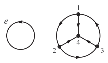
Figure 2.1. Oriented loop $e$ and oriented $K_{4}$

Lemma 2-2.

Let $n\geq 4$ be an integer and $G$ the graph which is a disjoint union of a loop $e$ and $K_{n}$. For every spatial graph $f(G)$ of $G$, the following holds:

(2.4) $$\sum_{\gamma\in\Gamma_{n}(K_{n})}{\rm lk}(f(e),f(\gamma))^{2}=\sum_{\gamma\in\Gamma_{n-1}(K_{n})}{\rm lk}(f(e),f(\gamma))^{2}.$$

Proof.

Let us prove (2.4) by induction on $n$. The case where $n=4$ is nothing other than Lemma 2-1. So we assume that $n>4$. Let $f(G)$ be a spatial graph of $G$. For a vertex $m$ of $K_{n}$ $(m=1,2,\ldots,n)$, we denote the subgraph obtained by removing $m$ and all edges incident to $m$ from $K_{n}$ by $K_{n-1}^{(m)}$. This subgraph is isomorphic to $K_{n-1}$, see the left figure in Fig. 2.2. Furthermore, for vertices $i,j$ and $m$ of $K_{n}$ such that $1\leq i<j\leq n$ and $i,j\neq m$, let $F_{ij}^{(m)}$ denote the subgraph obtained by removing the edge $\overline{ij}$ and $n-3$ edges $\overline{mk}$ $(1\leq k\leq n,\ k\neq i,j)$. This subgraph is not isomorphic to $K_{n-1}$ but is homeomorphic to it. Actually, $F_{ij}^{(m)}$ is obtained by replacing the edge $\overline{ij}$ in $K_{n-1}^{(m)}$ with the path $\overline{imj}$ of length $2$, see the right figure in Fig. 2.2. Then for the spatial subgraph $f(e\cup F_{ij}^{(m)})$, by the assumption we have

$$\sum_{\gamma\in\Gamma_{n}(F_{ij}^{(m)})}{\rm lk}(f(e),f(\gamma))^{2}+\sum_{\begin{subarray}{c}\gamma\in\Gamma_{n-1}(K_{n-1}^{(m)})\\ \overline{ij}\not\subset\gamma\end{subarray}}{\rm lk}(f(e),f(\gamma))^{2}$$

$$= \sum_{\begin{subarray}{c}\gamma\in\Gamma_{n-1}(F_{ij}^{(m)})\\ \overline{imj}\subset\gamma\end{subarray}}{\rm lk}(f(e),f(\gamma))^{2}+\sum_{\begin{subarray}{c}\gamma\in\Gamma_{n-2}(K_{n-1}^{(m)})\\ \overline{ij}\not\subset\gamma\end{subarray}}{\rm lk}(f(e),f(\gamma))^{2}.$$

Let us fix the vertex $m$ and add both sides of (2) for all $i,j$ such that $1\leq i<j\leq n$ and $i,j\neq m$. First, consider an $n$-cycle $\gamma$ of $K_{n}$ where the vertices $i$ and $j$ are adjacent to the vertex $m$ on $\gamma$. In this case, $\gamma$ is an $n$-cycle of $F_{ij}^{(m)}$ and we have

(2.6) $$\sum_{\begin{subarray}{c}1\leq i<j\leq n\\ i,j\neq m\end{subarray}}\bigg{(}\sum_{\gamma\in\Gamma_{n}(F_{ij}^{(m)})}{\rm lk}(f(e),f(\gamma))^{2}\bigg{)}=\sum_{\gamma\in\Gamma_{n}(K_{n})}{\rm lk}(f(e),f(\gamma))^{2}.$$

Next, consider an $(n-1)$-cycle $\gamma$ of $K_{n-1}^{(m)}$. Let $\overline{ij}$ be an edge of $K_{n-1}^{(m)}$ that is not contained in $\gamma$. Then there are $\binom{n-1}{2}-(n-1)=(n^{2}-5n+4)/2$ ways to choose such $i$ and $j$, and thus we have

$$\sum_{\begin{subarray}{c}1\leq i<j\leq n\\ i,j\neq m\end{subarray}}\bigg{(}\sum_{\begin{subarray}{c}\gamma\in\Gamma_{n-1}(K_{n-1}^{(m)})\\ \overline{ij}\not\subset\gamma\end{subarray}}{\rm lk}(f(e),f(\gamma))^{2}\bigg{)}$$

$$= \frac{n^{2}-5n+4}{2}\sum_{\gamma\in\Gamma_{n-1}(K_{n-1}^{(m)})}{\rm lk}(f(e),f(\gamma))^{2}.$$

Next, consider an $(n-1)$-cycle $\gamma$ of $K_{n}$ containing the vertex $m$, where the vertices $i$ and $j$ are adjacent to $m$ on $\gamma$. Then $\gamma$ is an $(n-1)$-cycle of $F_{ij}^{(m)}$ containing the path $\overline{imj}$ and we have

(2.8) $$\sum_{\begin{subarray}{c}1\leq i<j\leq n\\ i,j\neq m\end{subarray}}\bigg{(}\sum_{\begin{subarray}{c}\gamma\in\Gamma_{n-1}(F_{ij}^{(m)})\\ \overline{imj}\subset\gamma\end{subarray}}\!\!\!\!{\rm lk}(f(e),f(\gamma))^{2}\bigg{)} = \sum_{\begin{subarray}{c}\gamma\in\Gamma_{n-1}(K_{n})\\ m\subset\gamma\end{subarray}}\!\!\!\!{\rm lk}(f(e),f(\gamma))^{2}.$$

Finally, consider an $(n-2)$-cycle $\gamma$ of $K_{n-1}^{(m)}$. Let $\overline{ij}$ be an edge of $K_{n-1}^{(m)}$ that is not contained in $\gamma$. Then there are $\binom{n-1}{2}-(n-2)=(n^{2}-5n+6)/2$ ways to choose such $i$ and $j$, and thus we have

$$\sum_{\begin{subarray}{c}1\leq i<j\leq n\\ i,j\neq m\end{subarray}}\bigg{(}\sum_{\begin{subarray}{c}\gamma\in\Gamma_{n-2}(K_{n-1}^{(m)})\\ \overline{ij}\not\subset\gamma\end{subarray}}{\rm lk}(f(e),f(\gamma))^{2}\bigg{)}$$

$$= \frac{n^{2}-5n+6}{2}\sum_{\gamma\in\Gamma_{n-2}(K_{n-1}^{(m)})}{\rm lk}(f(e),f(\gamma))^{2}.$$

Furthermore, for each $f(K_{n-1}^{(m)})$, the following holds by the assumption:

(2.10) $$\sum_{\gamma\in\Gamma_{n-1}(K_{n-1}^{(m)})}{\rm lk}(f(e),f(\gamma))^{2}=\sum_{\gamma\in\Gamma_{n-2}(K_{n-1}^{(m)})}{\rm lk}(f(e),f(\gamma))^{2}.$$

Theorefore, from (2) and (2.6), (2), (2.8), (2), (2.10), we have

$$\sum_{\gamma\in\Gamma_{n}(K_{n})}{\rm lk}(f(e),f(\gamma))^{2}$$

$$= \sum_{\begin{subarray}{c}\gamma\in\Gamma_{n-1}(K_{n})\\ m\subset\gamma\end{subarray}}{\rm lk}(f(e),f(\gamma))^{2}+\sum_{\gamma\in\Gamma_{n-1}(K_{n-1}^{(m)})}{\rm lk}(f(e),f(\gamma))^{2}.$$

Then, let us add both sides of (2) for all $m=1,2,\ldots,n$. First, in the $(n-1)$-cycle $\gamma$ of $K_{n}$, there are $(n-1)$ ways to choose the vertex $m$ that is contained in $\gamma$. Thus we have

(2.12) $$\sum_{m=1}^{n}\bigg{(}\sum_{\begin{subarray}{c}\gamma\in\Gamma_{n-1}(K_{n})\\ m\subset\gamma\end{subarray}}\!\!\!\!{\rm lk}(f(e),f(\gamma))^{2}\bigg{)}=(n-1)\sum_{\gamma\in\Gamma_{n-1}(K_{n})}\!\!\!\!{\rm lk}(f(e),f(\gamma))^{2}.$$

Second, in the $(n-1)$-cycle $\gamma$ of $K_{n}$, for the vertex $m$ that is not contained in $\gamma$, the cycle $\gamma$ is an $(n-1)$-cycle of $K_{n-1}^{(m)}$. Since there is only one way to choose such an $m$, we have

(2.13) $$\sum_{m=1}^{n}\bigg{(}\sum_{\gamma\in\Gamma_{n-1}(K_{n-1}^{(m)})}{\rm lk}(f(e),f(\gamma))^{2}\bigg{)}=\sum_{\gamma\in\Gamma_{n-1}(K_{n})}{\rm lk}(f(e),f(\gamma))^{2}.$$

Then by substituting (2.12) and (2.13) into (2), we have

$$n\sum_{\gamma\in\Gamma_{n}(K_{n})}{\rm lk}(f(e),f(\gamma))^{2}=n\sum_{\gamma\in\Gamma_{n-1}(K_{n})}{\rm lk}(f(e),f(\gamma))^{2}.$$

This completes the proof. ∎

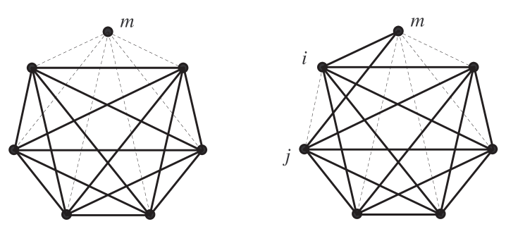
Figure 2.2. $K_{n-1}^{(m)}$ (left) and $F_{ij}^{(m)}$ (right) $(n=7)$

Corollary 2-3.

Let $n\geq 4$ be an integer and $G$ the graph which is a disjoint union of a loop $e$ and $K_{n}$. For every spatial graph $f(G)$ of $G$, the following holds:

(2.14) $$\sum_{\gamma\in\Gamma_{n}(K_{n})}{\rm lk}(f(e),f(\gamma))^{2}=(n-3)!\sum_{\gamma\in\Gamma_{3}(K_{n})}{\rm lk}(f(e),f(\gamma))^{2}.$$

Proof.

We denote the subgraph of $K_{n}$ obtained by removing exactly $k$ vertices $m_{1},m_{2},\ldots,m_{k}\ (1\leq k\leq n-1)$ and all edges incident to them from $K_{n}$ by $K_{n-k}^{(m_{1}m_{2}\cdots m_{k})}$. Note that this subgraph is isomorphic to $K_{n-k}$. Then by repeatedly using Lemma 2-2, we have

$$\sum_{\gamma\in\Gamma_{n}(K_{n})}{\rm lk}(f(e),f(\gamma))^{2}=\sum_{\gamma\in\Gamma_{n-1}(K_{n})}{\rm lk}(f(e),f(\gamma))^{2}$$

$$= \sum_{m_{1}=1}^{n}\bigg{(}\sum_{\gamma\in\Gamma_{n-1}(K_{n-1}^{(m_{1})})}{\rm lk}(f(e),f(\gamma))^{2}\bigg{)}$$

$$= \sum_{m_{1}=1}^{n}\bigg{(}\sum_{\gamma\in\Gamma_{n-2}(K_{n-1}^{(m_{1})})}{\rm lk}(f(e),f(\gamma))^{2}\bigg{)}=2\sum_{\gamma\in\Gamma_{n-2}(K_{n})}{\rm lk}(f(e),f(\gamma))^{2}$$

$$= 2\sum_{1\leq m_{1}<m_{2}\leq n}\bigg{(}\sum_{\gamma\in\Gamma_{n-2}(K_{n-2}^{(m_{1}m_{2})})}{\rm lk}(f(e),f(\gamma))^{2}\bigg{)}$$

$$= 2\sum_{1\leq m_{1}<m_{2}\leq n}\bigg{(}\sum_{\gamma\in\Gamma_{n-3}(K_{n-2}^{(m_{1}m_{2})})}{\rm lk}(f(e),f(\gamma))^{2}\bigg{)}$$

$$= 2\cdot 3\sum_{\gamma\in\Gamma_{n-3}(K_{n})}{\rm lk}(f(e),f(\gamma))^{2}=\cdots=k!\sum_{\gamma\in\Gamma_{n-k}(K_{n})}{\rm lk}(f(e),f(\gamma))^{2}.$$

So if we set $k=n-3$, we have the desired conclusion. ∎

Proof of Theorem 1-1.

For a $k$-cycle $\gamma$ of $K_{n}$, we denote the subgraph of $K_{n}$ obtained by removing all $k$ vertices of $\gamma$ and all edges incident to them from $K_{n}$ by $G_{\gamma}$. Note that this subgraph is isomorphic to $K_{n-k}$. Then we have

$$(1+\delta_{pq})\sum_{\lambda\in\Gamma_{p,q}(K_{n})}{\rm lk}(f(\lambda))^{2}$$

$$= \sum_{\gamma\in\Gamma_{p}(K_{n})}\bigg{(}\sum_{\gamma^{\prime}\in\Gamma_{q}(G_{\gamma})}{\rm lk}(f(\gamma),f(\gamma^{\prime}))^{2}\bigg{)}.$$

Then by Corollary 2-3, the right side of (2) can be expressed as follows:

$$\sum_{\gamma\in\Gamma_{p}(K_{n})}\bigg{(}\sum_{\gamma^{\prime}\in\Gamma_{q}(G_{\gamma})}{\rm lk}(f(\gamma),f(\gamma^{\prime}))^{2}\bigg{)}$$

$$= \sum_{\gamma\in\Gamma_{p}(K_{n})}\bigg{(}(q-3)!\sum_{\gamma^{\prime}\in\Gamma_{3}(G_{\gamma})}{\rm lk}(f(\gamma),f(\gamma^{\prime}))^{2}\bigg{)}$$

$$= (q-3)!\sum_{\gamma^{\prime}\in\Gamma_{3}(K_{n})}\bigg{(}\sum_{\gamma\in\Gamma_{p}(G_{\gamma^{\prime}})}{\rm lk}(f(\gamma),f(\gamma^{\prime}))^{2}\bigg{)}.$$

Let $H_{\gamma^{\prime}}^{i}\ (i=1,2,\ldots,l,\ l=\binom{n-3}{p})$ be the collection of all subgraphs of $G_{\gamma^{\prime}}$ that are isomorphic to $K_{p}$. Then the sets of $p$-cycles $\Gamma_{p}(H_{\gamma^{\prime}}^{i})$ are mutually disjoint, and their direct sum equals $\Gamma_{p}(G_{\gamma^{\prime}})$. Then by Corollary 2-3, we have

$$\sum_{\gamma^{\prime}\in\Gamma_{3}(K_{n})}\bigg{(}\sum_{\gamma\in\Gamma_{p}(G_{\gamma^{\prime}})}{\rm lk}(f(\gamma),f(\gamma^{\prime}))^{2}\bigg{)}$$

$$= \sum_{\gamma^{\prime}\in\Gamma_{3}(K_{n})}\bigg{(}\sum_{i=1}^{l}\bigg{(}\sum_{\gamma\in\Gamma_{p}(H_{\gamma^{\prime}}^{i})}{\rm lk}(f(\gamma),f(\gamma^{\prime}))^{2}\bigg{)}\bigg{)}$$

$$= \sum_{\gamma^{\prime}\in\Gamma_{3}(K_{n})}\bigg{(}\sum_{i=1}^{l}\bigg{(}(p-3)!\sum_{\gamma\in\Gamma_{3}(H_{\gamma^{\prime}}^{i})}{\rm lk}(f(\gamma),f(\gamma^{\prime}))^{2}\bigg{)}\bigg{)}$$

$$= (p-3)!\sum_{\gamma^{\prime}\in\Gamma_{3}(K_{n})}\bigg{(}\sum_{i=1}^{l}\bigg{(}\sum_{\gamma\in\Gamma_{3}(H_{\gamma^{\prime}}^{i})}{\rm lk}(f(\gamma),f(\gamma^{\prime}))^{2}\bigg{)}\bigg{)}.$$

Note that each $3$-cycle $\gamma$ of $G_{\gamma^{\prime}}$ is shared by exactly $\binom{n-6}{p-3}$ subgraphs $H_{\gamma^{\prime}}^{i}$’s. This implies that

(2.18) $$\sum_{i=1}^{l}\bigg{(}\sum_{\gamma\in\Gamma_{3}(H_{\gamma^{\prime}}^{i})}\!\!\!\!{\rm lk}(f(\gamma),f(\gamma^{\prime}))^{2}\bigg{)}=\binom{n-6}{p-3}\sum_{\gamma\in\Gamma_{3}(G_{\gamma^{\prime}})}\!\!\!\!{\rm lk}(f(\gamma),f(\gamma^{\prime}))^{2}.$$

Then it holds from (2), (2) and (2.18) that

$$\sum_{\gamma\in\Gamma_{p}(K_{n})}\bigg{(}\sum_{\gamma^{\prime}\in\Gamma_{q}(G_{\gamma})}{\rm lk}(f(\gamma),f(\gamma^{\prime}))^{2}\bigg{)}$$

$$= (p-3)!(q-3)!\binom{n-6}{p-3}\sum_{\gamma^{\prime}\in\Gamma_{3}(K_{n})}\bigg{(}\sum_{\gamma\in\Gamma_{3}(G_{\gamma^{\prime}})}{\rm lk}(f(\gamma),f(\gamma^{\prime}))^{2}\bigg{)}$$

$$= 2(n-6)!\sum_{\lambda\in\Gamma_{3,3}(K_{n})}{\rm lk}(f(\lambda))^{2}.$$

By (2), (2) and $2/(1+\delta_{pq})=2-\delta_{pq}$, we have the result. ∎

References

- [1] J. H. Conway and C. McA. Gordon, Knots and links in spatial graphs, J. Graph Theory 7 (1983), 445–453.
- [2] A. A. Kazakov and Ph. G. Korablev, Triviality of the Conway–Gordon function for spatial complete graphs, J. Math. Sci. (N.Y.) 203 (2014), 490–498.
- [3] H. Morishita and R. Nikkuni, Generalizations of the Conway–Gordon theorems and intrinsic knotting on complete graphs, J. Math. Soc. Japan 71 (2019), 1223–1241.
- [4] H. Morishita and R. Nikkuni, Generalization of the Conway–Gordon theorem and intrinsic linking on complete graphs, Ann. Comb. 25 (2021), 439–470.
- [5] R. Nikkuni, A refinement of the Conway–Gordon theorems, Topology Appl. 156 (2009), 2782–2794.
- [6] R. Nikkuni, Topology of Spatial Graphs (regarding the Conway–Gordon theorems), SGC Library 178, SAIENSU-SHA Co.,Ltd., 2022. (in Japanese)
- [7] H. Sachs, On spatial representations of finite graphs, Finite and infinite sets, Vol. I, II (Eger, 1981), 649–662, Colloq. Math. Soc. Janos Bolyai, 37, North-Holland, Amsterdam, 1984.
- [8] A. Yu. Vesnin and A. V. Litvintseva, On linking of hamiltonian pairs of cycles in spatial graphs (in Russian), Sib. Èlektron. Mat. Izv. 7 (2010), 383–393