LpBound: Pessimistic Cardinality Estimation using $\ell_{p}$-Norms of Degree Sequences

Abstract

Cardinality estimation is the problem of estimating the size of the output of a query, without actually evaluating the query. The cardinality estimator is a critical piece of a query optimizer, and is often the main culprit when the optimizer chooses a poor plan.

This paper introduces LpBound, a “pessimistic” cardinality estimator for multijoin queries (acyclic or cyclic) with selection predicates and group-by clauses. LpBound computes a guaranteed upper bound on the size of the query output using simple statistics on the input relations, consisting of $\ell_{p}$-norms of degree sequences. The bound is the optimal solution of a linear program whose constraints encode data statistics and Shannon inequalities. We introduce two optimizations that exploit the structure of the query in order to speed up the estimation time and make LpBound practical.

We experimentally evaluate LpBound against a range of traditional, pessimistic, and machine learning-based estimators on the JOB, STATS, and subgraph matching benchmarks. Our main finding is that LpBound can be orders of magnitude more accurate than traditional estimators used in mainstream open-source and commercial database systems. Yet it has comparable low estimation time and space requirements. When injected the estimates of LpBound, Postgres derives query plans at least as good as those derived using the true cardinalities.

Keywords

Cardinality Estimation, Degree Sequence, Lp-norms

1 Introduction

The Cardinality Estimation problem, or CE for short, is to estimate the output size of a query using only simple, precomputed statistics on the database. CE is one of the oldest and most important problems in databases and data management. It is used as the primary metric guiding cost-based query optimization, for making decisions about every aspect of query execution, ranging from broad logical optimizations like the join order, to deciding the number of servers to distribute the data over, and to detailed physical optimizations, like the use of bitmap filters and memory allocation for hash tables.

Unfortunately, CE is notoriously difficult, and this affects significantly the performance of data management systems. Current systems use density-based estimators, which were pioneered by System R [28]. They make drastic simplifying assumptions (uniformity, independence, containment of values, and preservation of values), and when the query has many joins and many predicates, then they tend to have large errors, leading to poor decisions by the downstream system; for example, the independence assumption often leads to major underestimation [25]. Density-based CE also has limited support for queries with group-by: most existing systems yield poor estimates for the number of distinct groups [12]. Yet the main problem with traditional CE is that it does not come with any theoretical guarantees about its estimate: it may under-, or over-estimate, by a little or by a lot, without any warning. Several studies have shown repeatedly that errors in the cardinality estimator can significantly degrade the performance of most advanced database systems [25, 23]. To escape the simplifying assumptions of density-based CE, several estimators were put forward that learn a model of the underlying distribution in the database, e.g., [18, 33, 34, 37]. This is a promising line of work, yet as previously reported (and shown in our experiments), their deployability is poor [32] as they lack explainability, have very slow training time, large model size, and are difficult to transfer with comparable accuracy from one workload to new workloads. One reason for this is that they need to de-normalize the joined relations and add up to exponentially many extra columns to represent new features. Cardinality estimation thus remains one of the major open challenges in data management.

In this paper, we introduce LpBound, a cardinality estimator that offers a one-sided guarantee: the true cardinality is guaranteed to be below that returned by LpBound. That is, LpBound returns a guaranteed upper bound on the size of the query output. Moreover, LpBound can explain the computed upper bound in terms of a simple inequality, called a q-inequality. This one-sided guarantee can be of use in many applications, for example it can guarantee that a query does not run out of memory, or it can put an upper bound on the number of servers required to distribute the output data. The challenge with this approach is to not overestimate too much. In other words, we want to reduce this upper bound as much as possible, while still maintaining the theoretical one-sided guarantee. To achieve that, we introduce novel statistics on the database, and demonstrate that they lead to strictly improved upper bounds. As an extra bonus, LpBound applies equally well to group-by queries.

There have been a small number of implementations that compute upper bounds on the cardinality, commonly called pessimistic cardinality estimation, or PCE for short [6, 7, 27]. However, these systems were limited because they used only two types of statistics on the input data: relation cardinalities, $|R|$, and maximum degree (a.k.a. maximum frequency) of an attribute $R.X$: if the values of $R.X$ are $x_{1},\ldots,x_{N}$, then the maximum degree is $\max_{i}|\sigma_{X=x_{i}}(R)|$. By using only limited input statistics, these first-generation PCE systems led to significant overestimates, and had worse accuracy than traditional, density-based CE systems.

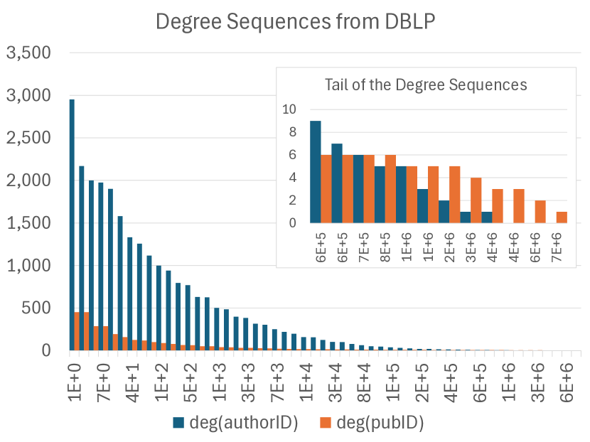
Figure 1: The Authors-Publication relationship in DBLP (in 2023) with $24\cdot 10^{6}$ records pairing $3.6\cdot 10^{6}$ authors and $7.1\cdot 10^{6}$ publications. The figure shows the degree sequences $\texttt{deg}(\texttt{authorID})$ and $\texttt{deg}(\texttt{pubID})$: The latter starts with a lower maximum degree, but has a longer tail (see inset). The author with rank 1 is H. Vincent Poor ($2951$ publications) and the publication with rank 1 is [29] (with $450$ authors).

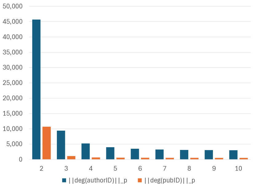
Figure 2: Instead of storing the two degree sequences, LpBound stores only some of their $\ell_{p}$-norms, for example for $p\in\{1,\ldots,10,\infty\}$ shown here. We do not show $\ell_{1}$ (it is equal to the cardinality $24\cdot 10^{6}$) and $\ell_{\infty}$ (it is the maximum degree, $2951$ or $450$ respectively). When $p$ ranges from $1$ to $\infty$, the $\ell_{p}$-norm ranges from the relation’s cardinality to the maximum degree of any value.

To achieve better upper bounds, we use significantly richer statistics on the input database. Concretely, we use the $\ell_{p}$-norms of degree sequences as inputs to LpBound. The degree sequence of an attribute $R.X$ is the sequence $\texttt{deg}_{R}(X)=(d_{1},d_{2},\ldots,d_{N})$, sorted in decreasing order, where $d_{i}$ is the frequency of the value $x_{i}$. The $\ell_{p}$-norm is $\left(\sum_{i}d_{i}^{p}\right)^{1/p}$. The $\ell_{p}$-norms of degree sequences are related to frequency moments [4]: The $p$’th frequency moment is $\sum_{i}d_{i}^{p}$. These are commonly used in statistics and machine learning, since they capture important information about the data distribution. This information can be very useful for cardinality estimation too. It is also practical as it can be computed and maintained efficiently [4]. Yet, to the best of our knowledge, the $\ell_{p}$-norms (or frequency moments) have not been used before for cardinality estimation. LpBound is, to the best of our knowledge, the first to use them for cardinality estimation. Fig. 2 shows the degree sequences of the Author-Publication relationship in the DBLP database, and Fig. 2 shows some of their $\ell_{p}$-norms.

LpBound takes as input a query with equality joins, equality and range predicates, and group-by clause, and computes an upper bound on the query output size, by using precomputed $\ell_{p}$-norms on the input database. LpBound offers a strong, theoretical guarantee: for any database that satisfies the given statistics, the query output size is guaranteed to be below the bound returned by LpBound. The bound is tight, in the sense that, if all we know about the input database are the given statistics, then there exists a worst-case input database with these statistics on which the query output is as large as the bound returned by LpBound. Finally, LpBound is able to explain the upper bound, in terms of a simple q-inequality relating the output size to the input statistics.

Contributions

In this paper we make four main contributions.

1. We introduce LpBound, a PCE that uses $\ell_{p}$-norms of input relations (Sec. 3). LpBound is a principled framework to compute the upper bound, based on information theory, building upon, and expanding a long line of theoretical results [5, 14, 2, 3, 1]. We show how to extend previous results to accommodate group-by queries. LpBound works for both cyclic and acyclic queries, and therefore can be used as an estimator both for traditional SQL workloads, which tend to be acyclic, and for graph pattern matching or SparQL queries, which tend to be cyclic.

2. We describe how to use most common values and histograms to extend LpBound to conjunctions and disjunctions of equality and range predicates (Sec. 5). To support predicates, LpBound uses data structures that are very similar to those used by SQL engines, and therefore LpBound could be easily incorporated in those systems.

3. We introduce two optimization techniques for computing the upper bound, which run in polynomial time in the size of the query and the number of available statistics (Sec. 4). One works for acyclic queries only, while the other works for arbitrary conjunctive queries albeit on one-column degree sequences. These techniques are essential for the practicality of LpBound, as cardinality estimation is often invoked thousands of times during query optimization, and it must run in times measured in milliseconds.

4. We conduct an extensive experimental evaluation of LpBound on real and synthetic workloads (Sec. 6). LpBound can be orders of magnitude more accurate than traditional estimators used in mainstream open-source and commercial database systems. Yet it has low estimation time and space requirements to remain practical. When injected the estimates of LpBound, Postgres derives query plans at least as good as those derived using the true cardinalities.

Related Work

Our paper builds on a long line of theoretical results that proved upper bounds on the size of the query output. The first such result appeared in a landmark paper by Atserias, Grohe, and Marx [5], which proved an upper bound in terms of the cardinalities of the input relations, known today as the AGM Bound. The AGM bound is not practical for real SQL workloads, which consist almost exclusively of acyclic queries, where the AGM bound is too large. For example, the AGM bound of a 2-way join is $|R\Join S|\leq|R|\cdot|S|$. The AGM bound was extended to account for functional dependencies [14, 2], and further extended to use the maximum degrees of attributes [3]: we refer to the latter as the max-degree bound. This line of work relies on information theory. A simplified version of the max-degree bound was incorporated into two pessimistic cardinality estimators [6, 16]. However, cardinalities and maximum degrees alone are still too limited to infer useful upper bounds for acyclic queries. For example, the max-degree bound of a 2-way join is $|R\Join_{X=Y}S|\leq\min(a\cdot|S|,|R|\cdot b)$, where $a$ is the maximum degree of $R.X$ and $b$ is the maximum degree of $S.Y$. Real data is often skewed and the maximum degree is large (the maximum degrees are $2951$ and $450$ in Fig. 2), and this led to large overestimates for more complex queries.

The first system to use degree sequences for pessimistic cardinality estimation was SafeBound [10, 9]. Since the degree sequences are often too large, SafeBound uses a lossy compression of them. It relies solely on combinatorics, it is limited to Berge-acyclic queries (see Sec. 2), and it does not support group-by. LpBound can be seen as a significant extension of SafeBound. By using information theory instead of combinatorics, LpBound computes the bound using $\ell_{p}$-norms, without requiring the degree sequences, and also works for cyclic queries and queries with group-by.

2 Background

Relations

We write $\texttt{Attrs}(R)$ for the set of attributes of a relation $R$. The domain of attributes $U\subseteq\texttt{Attrs}(R)$ is $\textsf{Dom}(R.U)\stackrel{{\scriptstyle\text{def}}}{{=}}\Pi_{U}(R)$.

Queries

LpBound supports single-block SQL queries:

SELECT [groupby-attrs]

$$\texttt{FROM }R_{1},R_{2},\ldots,R_{m}$$

WHERE [join-and-selection-predicates]

GROUP BY [groupby-attrs]

We ignore aggregates in SELECT because they do not affect the output cardinality. We do not support sub-queries. The predicates can be equality, range, and their conjunction and disjunction; IN and LIKE predicates can be supported with trivial effort (see Sec. 5). Queries with bag semantics are also supported, by replacing them with a full query. For example, the output of $\texttt{SELECT A FROM }\ldots$ (without GROUP BY) is a bag that has the same size as the output of $\texttt{SELECT * FROM }\ldots$, which is a set. Throughout the paper we will assume that queries have set semantics. We will use the conjunctive query notation instead of SQL:

$$Q(V_{0})= R_{1}(V_{1})\wedge R_{2}(V_{2})\wedge\cdots\wedge R_{m}(V_{m})\wedge\text{[predicates]}$$ (1)

where each $V_{j}\stackrel{{\scriptstyle\text{def}}}{{=}}\texttt{Attrs}(R_{j})$ is a set of variables, and $V_{0}\subseteq V_{1}\cup\cdots\cup V_{m}$ represents the group-by variables. We denote by $\texttt{Vars}(Q)\stackrel{{\scriptstyle\text{def}}}{{=}}V_{1}\cup\cdots\cup V_{m}=\{X_{1},\ldots,X_{n}\}$ the set of all variables in the query. When $V_{0}=\{X_{1},\ldots,X_{n}\}$, then we say that $Q$ is a full conjunctive query. $Q$ is acyclic if its relations $R_{1},\ldots,R_{m}$ can be placed on the nodes of a tree, such that, for every individual variable $X_{i}$, the set of tree nodes that contain $X_{i}$ forms a connected component. $Q$ is called Berge-acyclic if it is acyclic and any two relations share at most one variable. For example, the 3-way join query $J_{3}$ is Berge-acyclic, while the 3-clique query $C_{3}$ is cyclic:

$$J_{3}(X,Y,Z,U)= R(X,Y)\wedge S(Y,Z)\wedge T(Z,U)$$ (2)

$$C_{3}(X,Y,Z)= R(X,Y)\wedge S(Y,Z)\wedge T(Z,X)$$ (3)

Degree Sequences

Fix a relation instance $R$, and two sets of variables $X,Y\subseteq\texttt{Attrs}(R)$. The degree sequence from $X$ to $Y$ in $R$ is the sequence $\texttt{deg}_{R}(Y|X)\stackrel{{\scriptstyle\text{def}}}{{=}}(d_{1},d_{2},\ldots,d_{N})$ obtained as follows. Compute the domain of $X$, $\textsf{Dom}(R.X)=\{x_{1},\ldots,x_{N}\}$, denote by $d_{i}=|\sigma_{X=x_{i}}(\Pi_{XY}(R))|$ the degree (or frequency) of $x_{i}$, and sort the values in the domain $\textsf{Dom}(R.X)$ such that their degrees are decreasing $d_{1}\geq d_{2}\geq\cdots\geq d_{N}$. We call $i$ the rank of the element $x_{i}$. Notice that $\texttt{deg}_{R}(Y|X)$ and $\texttt{deg}_{R}(XY|X)$ are the same, where $XY$ denotes the union $X\cup Y$. When $X=\emptyset$, then the degree sequence has length 1, $\texttt{deg}_{R}(Y|\emptyset)=(|\textsf{Dom}(R.Y)|)$. When the functional dependency $X\rightarrow Y$ holds (for example, if $X$ is a key), then $\texttt{deg}_{R}(Y|X)=(1,1,\ldots,1)$. When $|X|\leq 1$, then we say that the degree sequence is simple, and when $XY=\texttt{Attrs}(R)$, then we say that the degree sequence is full and denote it by $\texttt{deg}_{R}(*|X)$, or just $\texttt{deg}_{R}(X)$ (we used this notation in Fig. 2). In this paper we will consider only simple degree sequences. The degree sequence also applies to the case when $R$ is a bag, not necessarily a set. The $\ell_{p}$-norm of a sequence $\bm{d}=(d_{1},d_{2},\ldots)$ is $||\bm{d}||_{p}\stackrel{{\scriptstyle\text{def}}}{{=}}\left(\sum_{i}d_{i}^{p}\right)^{1/p}$, where $p\in(0,\infty]$. When $p$ increases towards $\infty$, $||\bm{d}||_{p}$ decreases and converges to $||\bm{d}||_{\infty}\stackrel{{\scriptstyle\text{def}}}{{=}}\max_{i}d_{i}$, see Fig. 2.

Fig. 3 illustrates some simple examples of degree sequences: $\texttt{deg}_{R}(YZ|X)$ is both simple and full, and we can write it as $\texttt{deg}_{R}(*|X)$ or just $\texttt{deg}_{R}(X)$. The degree sequence $\texttt{deg}_{R}(Z|XY)$ is not simple.

$$R= \begin{array}[c]{|c|c|c|}\hline\cr X&Y&Z\\ \hline\cr 1&a&\ldots\\ 1&b&\ldots\\ 1&b&\ldots\\ 2&a&\ldots\\ 2&b&\ldots\\ 3&b&\ldots\\ 3&c&\ldots\\ 4&d&\ldots\\ \hline\cr\end{array} \begin{array}[c]{ll}\texttt{deg}_{R}(YZ|X)&=(3,2,2,1)\\ \texttt{deg}_{R}(Y|X)&=(2,2,2,1)\\ \texttt{deg}_{R}(Z|XY)&=(2,1,1,1,1,1,1)\\ \texttt{deg}_{R}(XYZ|\emptyset)&=(8)=(|R|)\end{array}$$

Figure 3: Examples of Degree Sequences.

Density-based CE

The traditional, density-based cardinality estimator [13] is limited to selections and joins. It makes the assumptions mentioned in the introduction and computes the estimate bottom-up on the query plan, for example:

$$\textsc{Est}(\sigma_{X=\text{value}}(R))= \frac{|R|}{|\textsf{Dom}(R.X)|}$$

$$\textsc{Est}(R\Join_{X=Y}S)= \frac{|R|\cdot|S|}{\max(|\textsf{Dom}(R.X)|,|\textsf{Dom}(S.Y)|)}$$

The ratio $\frac{|R|}{|\textsf{Dom}(R.X)|}$ is the average degree, $\texttt{Avg}(\texttt{deg}_{R}(*|X))$.

Queries with group-by are treated differently by different systems. We describe briefly how they are handled by two open-source systems, illustrating on the following group-by query:

$$JG_{3}(X,U)= R(X,Y)\wedge S(Y,Z)\wedge T(Z,U)$$ (4)

DuckDB ignores the group-by clause, and estimates the size of $JG_{3}$ to be the same as that of the full join $J_{3}$ (Eq. (2)). Postgres estimates it as the minimum between the full join, and the product of the domains of the group-by variables, $|\textsf{Dom}(R.X)|\cdot|\textsf{Dom}(T.U)|$.

Theoretical Upper Bounds

An upper bound for a conjunctive query $Q$ is a numerical value, which is computed in terms of statistics on the input database, such as the output size of the query is is guaranteed to be below that bound. The upper bound is tight if there exists a database instance, satisfying the statistics, such that the query’s output is as large as the bound. The AGM bound [5] is a tight upper that uses only the cardinalities $|R_{1}|,\ldots,|R_{m}|$; in other words, it uses only the $\ell_{1}$-norms of full degree sequences. A non-negative sequence $w_{1},\ldots,w_{m}$ is called a fractional edge cover of the query $Q$ in Eq. (1) if every variable $X_{i}$ is “covered”, meaning that $\sum_{j\in[m]:X_{i}\in V_{j}}w_{j}\geq 1$. The AGM bound states that $|Q|\leq|R_{1}|^{w_{1}}\cdot|R_{2}|^{w_{2}}\cdots|R_{m}|^{w_{m}}$ for any fractional edge cover. It is useful for cyclic queries like $C_{3}$ above (see Sec. 3.1), but for acyclic queries it degenerates to a product of cardinalities, because the optimal edge cover is integral. For example, the AGM bound of the 3-way join in Eq. (2) is $|J_{3}|\leq|R|\cdot|T|$, because the optimal fractional edge cover is $w_{R}=1,w_{S}=0,w_{T}=1$.

The max-degree bound introduced in [3] generalizes the AGM bound by using both cardinalities and maximum degrees; in other words, it uses both $\ell_{1}$ and $\ell_{\infty}$ norms of degree sequences. When restricted to acyclic queries, the max-degree bound represents an improvement over the AGM, but it is still less accurate than a density-based estimate. For example, the bound for $J_{3}$ is the minimum of the following four quantities (see also [7]):

$$|J_{3}|\leq |R|\cdot|T|$$

$$|J_{3}|\leq |R|\cdot||\texttt{deg}_{S}(Z|Y)||_{\infty}\cdot||\texttt{deg}_{T}(U|Z)||_{\infty}$$ (5)

$$|J_{3}|\leq |S|\cdot||\texttt{deg}_{R}(X|Y)||_{\infty}\cdot||\texttt{deg}_{T}(U|Z)||_{\infty}$$

$$|J_{3}|\leq |T|\cdot||\texttt{deg}_{S}(Y|Z)||_{\infty}\cdot||\texttt{deg}_{R}(X|Y)||_{\infty}$$

For comparison, the traditional, density-based estimator for $J_{3}$ is:

$$\textsc{Est}(J_{3})= \frac{|R|\cdot|S|\cdot|T|}{\max(|\textsf{Dom}(R.Y)|,|\textsf{Dom}(S.Y)|)\cdot\max(|\textsf{Dom}(S.Z)|,|\textsf{Dom}(T.Z)|)}$$

When $|\textsf{Dom}(R.Y)|\leq|\textsf{Dom}(S.Y)|$ and $|\textsf{Dom}(S.Z)|\leq|\textsf{Dom}(T.Z)|$ then the estimator becomes $|R|\cdot\texttt{Avg}(\texttt{deg}_{S}(Z|Y))\cdot\texttt{Avg}(\texttt{deg}_{T}(U|Z))$, which is the same as the max-degree bound in Eq. (5) with the maximum degree replaced by the average degree.

SafeBound [9, 10] uses simple, full degree sequences and computes a tight upper bound of a Berge-acyclic, full conjunctive query. For example, if $\texttt{deg}_{R}(*|X)=(a_{1}\geq a_{2}\geq\cdots)$ and $\texttt{deg}_{S}(*|Y)=(b_{1}\geq b_{2}\geq\cdots)$, then SafeBound will infer the following bound on a 2-way join: $|R\Join_{X=Y}S|\leq\sum_{i}a_{i}b_{i}$. When applied to the 3-way join $J_{3}$ SafeBound returns a much better bound than the degree bound (5), but that bound is not described by a closed-form formula; it is only given by an algorithm. The limitations of SafeBound are its lack of explainability, its restriction to Berge-acyclic queries, and its reliance on compression heuristics for the degree sequences.

Information Theory

Let $X$ be a finite random variable, with outcomes $x_{1},\ldots,x_{N}$, and probability function $\mathop{\textnormal{Pr}}$. Its entropy is:

$$h(X)\stackrel{{\scriptstyle\text{def}}}{{=}} -\sum_{i=1,N}\mathop{\textnormal{Pr}}(x_{i})\log\mathop{\textnormal{Pr}}(x_{i})$$

where $\log$ is in base 2. It holds that $0\leq h(X)\leq\log N$, and $h(X)=\log N$ iff $\mathop{\textnormal{Pr}}$ is uniform, i.e., $\mathop{\textnormal{Pr}}(x_{1})=\cdots=\mathop{\textnormal{Pr}}(x_{N})=1/N$.

Let $X_{1},\ldots,X_{n}$ be $n$ finite, jointly distributed random variables. They can be described by a finite relation $R(X_{1},\ldots,X_{n})$, representing their support, and a probability function s.t. for each tuple $t\in R$, $\mathop{\textnormal{Pr}}(t)\geq 0$ and $\sum_{t\in R}\mathop{\textnormal{Pr}}(t)=1$. For every subset $U$ of variables, $h(U)$ denotes the entropy of the marginal distribution of the random variables in $U$. For example, we have $h(X_{1}X_{3})$, $h(X_{2}X_{4}X_{5})$, etc. This defines a vector $h$ with $2^{n}$ dimensions, which is called an entropic vector. The conditional entropy is defined as

$$h(V|U)\stackrel{{\scriptstyle\text{def}}}{{=}} h(UV)-h(U)$$ (6)

The following hold for all subsets of variables $U,V\subseteq\texttt{Attrs}(R)$:

$$h(V)\leq \log|\textsf{Dom}(R.V)| h(V|U)\leq \log||\texttt{deg}_{R}(V|U)||_{\infty}$$ (7)

Every entropic vector $\bm{h}$ satisfies the basic Shannon inequalities:

$$h(\emptyset)= \ 0$$

Monotonicity: $$h(U\cup V)\geq \ h(U)$$ (8)

Submodularity: $$h(U)+h(V)\geq \ h(U\cup V)+h(U\cap V)$$ (9)

Every vector $\bm{h}$ that satisfies the basic Shannon inequalities is called a polymatroid. Every entropic vector is a polymatroid, but the converse is not true [36, 35].

3 The LpBound Cardinality Estimator

Our system, LpBound, is a significant extension of previous upper bound estimators, in that it computes a tight upper bound of the query $Q$ by using $\ell_{p}$-norms of simple degree sequences. LpBound can explain its upper bound in terms of a simple inequality, called a q-inequality. We introduce LpBound gradually, by first describing the q-inequalities, and showing later how to compute the optimal bound. Throughout this section, we assume that the query has no predicates: we discuss predicates in Sec. 5.

3.1 Q-Inequalities for Full Queries

For upper bounds on a full conjunctive query in terms of $\ell_{p}$-norms, we use inequalities described in [1]. As a simple warmup, consider the 2-way join, which we write as:

$$J_{2}(X,Y,Z)= R(X,Y)\wedge S(Y,Z)$$ (10)

LpBound uses the following q-inequalities:

$$|J_{2}|\leq |R|\cdot|S|$$ (11)

$$|J_{2}|\leq |R|\cdot||\texttt{deg}_{S}(*|Y)||_{\infty}$$ (12)

$$|J_{2}|\leq ||\texttt{deg}_{R}(*|Y)||_{\infty}\cdot|S|$$ (13)

$$|J_{2}|\leq ||\texttt{deg}_{R}(*|Y)||_{2}\cdot||\texttt{deg}_{S}(*|Y)||_{2}$$ (14)

The first bound is the AGM bound; the next two are the max-degree bound, and are always lower (i.e. better) than the AGM bound. The last bound is new, and follows from the Cauchy-Schwartz inequality. LpBound always returns the smallest value of all q-inequalities. It does not need to enumerate all of them; instead it computes the bound differently (explained below in Sec. 3.4), then returns as explanation the single q-inequality that produces that bound.

For the 3-way join $J_{3}$ from Eq. (2), LpBound uses many more q-inequalities. It includes all those considered by the max-degree bound (Eq. (5)) and many more. We show here only two q-inequalities:

$$|J_{3}|\leq ||\texttt{deg}_{R}(X|Y)||_{2}\cdot|S|^{1/2}\cdot||\texttt{deg}_{T}(U|Z)||_{2}$$

$$|J_{3}|\leq |R|^{1/3}\cdot||\texttt{deg}_{R}(X|Y)||_{2}^{2/3}\cdot||\texttt{deg}_{S}(Z|Y)||_{2}^{2/3}\cdot||\texttt{deg}_{T}(U|Z)||_{3}$$ (15)

To the best of our knowledge, such inequalities have not been used previously in cardinality estimation. We prove (15) in Sec. 3.3. LpBound also improves significantly the bounds of cyclic queries, for example it considers these q-inequalities for the 3-clique $C_{3}$:

$$|C_{3}|\leq \left(|R|\cdot|S|\cdot|T|\right)^{1/2}$$

$$|C_{3}|\leq \left(||\texttt{deg}_{R}(Y|X)||_{2}^{2}\cdot||\texttt{deg}_{S}(Z|Y)||_{2}^{2}\cdot||\texttt{deg}_{T}(X|Z)||_{2}^{2}\right)^{1/3}$$

$$|C_{3}|\leq \left(||\texttt{deg}_{R}(Y|X)||_{3}^{3}\cdot||\texttt{deg}_{S}(Y|Z)||_{3}^{3}\cdot|T|^{5}\right)^{1/6}$$ (16)

The first is the AGM bound corresponding to the fractional edge cover $w_{R}=w_{S}=w_{T}=\frac{1}{2}$. The other two are novel and surprising.

3.2 LpBound for group-by Queries

Similar q-inequalities hold for queries with group-by. We illustrate here for the query $JG_{3}$ in Eq. (4).

Every q-inequality that holds for the full conjunctive query also holds for the group-by query, in other words $|JG_{3}|\leq|J_{3}|$, and all upper bounds for $J_{3}$ also apply to $JG_{3}$; this is used by DuckDB.

Further q-inequalities can be obtained by dropping variables that do not occur in group-by, as done in Postgres. For example, we can drop the variables $Y,Z$ from $JG_{3}$ and obtain the query:

$$JG_{3}^{\prime}(X,U)= R^{\prime}(X)\wedge T^{\prime}(U)$$

for which we can infer:

$$|JG_{3}|\leq |JG_{3}^{\prime}|\leq|R^{\prime}|\cdot|T^{\prime}|=|\textsf{Dom}(R.X)|\cdot|\textsf{Dom}(T.U)|$$

However, LpBound uses many more q-inequalities, which are not necessarily derived using the two heuristics above. For example, consider the following star-join with group-by:

$$\text{StarG}(X_{1},X_{2})= R_{1}(X_{1},Z)\wedge R_{2}(X_{2},Z)\wedge S(Y,Z)$$

LpBound infers (among others) the following inequality:

$$|\text{StarG}|\leq |S|^{1/3}\cdot||\texttt{deg}_{R_{1}}(X_{1}|Z)||_{3}\cdot||\texttt{deg}_{R_{2}}(X_{2}|Z)||_{3}$$ (17)

This q-inequality does not hold for the full conjunctive query and it involves all query variables. We prove (17) below.

3.3 Proofs of Q-Inequalities

Consider $n$ finite random variables $X_{1},\ldots,X_{n}$, and let their set of outcomes be the relation $R(X_{1},\ldots,X_{n})$ (see Sec. 2). Then, for any subsets of variables $U,V\subseteq\texttt{Attrs}(R)$ and any $p\in(0,\infty]$, the following holds [1]:

$$\frac{1}{p}h(U)+h(V|U)\leq \log||\texttt{deg}_{R}(V|U)||_{p}$$ (18)

Inequalities (7) are special cases of (18), where $p=1$ or $p=\infty$.

Inequality (18) is very important. It connects an information-theoretic term in the LHS with a statistics on the input database in the RHS. All q-inequalities inferred by LpBound follow from (18) and the basic Shannon inequalities. We illustrate with two examples.

First, we prove the q-inequality (15) for $J_{3}$. Assume three input relations $R(X,Y)$, $S(Y,Z)$, $T(Z,U)$, and denote by $N\stackrel{{\scriptstyle\text{def}}}{{=}}|J_{3}|$ the size of the query’s output. Consider the uniform probability distribution with outcomes $J_{3}$: every tuple $t=(x,y,z,u)\in J_{3}$ has the same probability, $\mathop{\textnormal{Pr}}(t)=1/N$. Therefore, their entropy is $h(XYZU)=\log|J_{3}|$ (by uniformity), and (15) follows from:

$$\log |R|+2\log||\texttt{deg}_{R}(X|Y)||_{2}+2\log||\texttt{deg}_{S}(Z|Y)||_{2}+3\log||\texttt{deg}_{T}(U|Z)||_{3}\geq$$

$$\geq h(XY)+2\left(\frac{1}{2}h(Y)+h(X|Y)\right)+2\left(\frac{1}{2}h(Y)+h(Z|Y)\right)+3\left(\frac{1}{3}h(Z)+h(U|Z)\right)\text{\hskip 5.69054ptby~\eqref{eq:h:p}}$$

$$= h(XY)+\left(h(XY)+h(X|Y)\right)+\left(h(YZ)+h(Z|Y)\right)+\left(h(UZ)+2h(U|Z)\right)\text{\hskip 17.07164ptby~\eqref{eq:chain}}$$

$$= \left(h(XY)+h(Z|Y)+h(U|Z)\right)+\left(h(XY)+h(UZ)\right)+\left(h(X|Y)+h(YZ)+h(U|Z)\right)$$

$$\geq \left(h(XY)+h(Z|XY)+h(U|XYZ)\right)+h(XYZU)+\left(h(X|YZ)+h(YZ)+h(U|XYZ)\right)$$

                 by submodularity

$$= 3h(XYZU)=3\log|J|$$

The first inequality is an application of (18). The second inequality uses submodularity, for example $h(Z|Y)\geq h(Z|XY)$ follows from $h(YZ)-h(Y)\geq h(XYZ)-h(XY)$, or $h(XY)+h(YZ)\geq h(XYZ)+h(Y)$.

Second, we prove the q-inequality (17). The setup is similar: assume some input relation instances
$R_{1}(X_{1},Z),R_{2}(X_{2},Z),S(Y,Z)$, let $\text{StarG}(X_{1},X_{2})$ be the output of the query, and denote by $N\stackrel{{\scriptstyle\text{def}}}{{=}}|\text{StarG}|$. Define $\text{Star}(X_{1},X_{2},Y,Z)$ to be the result of the full join. We need a probability distribution on Star whose marginal on $X_{1},X_{2}$ is uniform. There are many ways to define such a distribution, we consider the following. Order the tuples in Star arbitrarily; then, for each tuple $t=(x_{1},x_{2},y,z)$, if there exists some earlier tuple with the same values $x_{1},x_{2}$ then set $\mathop{\textnormal{Pr}}(t)=0$, otherwise set $\mathop{\textnormal{Pr}}(t)=1/N$. At this point, we continue similarly to the previous example:

$$\frac{1}{3}\log |S|+\log||\texttt{deg}_{R_{1}}(X_{1}|Z)||_{3}+\log||\texttt{deg}_{R_{2}}(X_{2}|Z)||_{3}\geq$$

$$\geq \frac{1}{3}h(YZ)+\frac{1}{3}h(Z)+h(X_{1}|Z)+\frac{1}{3}h(Z)+h(X_{2}|Z)$$

$$\geq \frac{1}{3}h(Z)+\frac{1}{3}h(Z)+h(X_{1}|Z)+\frac{1}{3}h(Z)+h(X_{2}|Z)$$

$$= h(Z)+h(X_{1}|Z)+h(X_{2}|Z)=h(X_{1}Z)+h(X_{2}|Z)$$

$$\geq h(X_{1}Z)+h(X_{2}|X_{1}Z)=h(X_{1}X_{2}Z)\geq h(X_{1}X_{2})=\log|\text{StarG}|$$

3.4 $\texttt{LP}_{\text{base}}$: The Basic Algorithm of LpBound

LpBound takes as input a query $Q$ (Eq. (1)) and a set of statistics on the input database consisting of $\ell_{p}$-norms on degree sequences, and returns: (1) a numerical upper bound $B$ such that $|Q|\leq B$ whenever the input database satisfies these statistics; (2) an explanation consisting of a q-inequality on $|Q|$, which, for the particular numerical values of the $\ell_{p}$-norms implies $|Q|\leq B$; and (3) a proof of the Shannon inequality needed to prove the q-inequality. For that, LpBound solves a Linear Program (LP) called $\texttt{LP}_{\text{base}}$ defined as follows:

The Real-valued Variables are all unknowns $h(U)\geq 0$, $\forall U\subseteq\texttt{Vars}(Q)$ ($2^{n}$ real-valued variables).

The Objective is to maximize $h(V_{0})$, where $V_{0}$ is the set of the group-by variables of the query in Eq. (1), under the following two types of constraints.

The Statistics Constraints are linear constraints of the form in Eq. (18), one for each $\ell_{p}$-norm of a degree sequence that has been computed on the input database.

The Shannon Constraints are all basic Shannon inequalities, as linear constraints (Eq. (8) and (9)).

LpBound uses the off-the-shelf solver HiGHS 1.7.2 [19] to solve both $\texttt{LP}_{\text{base}}$ and its dual linear program. The optimal solution of $\texttt{LP}_{\text{base}}$ consists of $2^{n}$ values $h^{*}(U)$, one for each set of query variables $U$. The optimal solution of the dual consists of non-negative weights $w^{*}\geq 0$, one for every statistics constraint, and non-negative weights $s^{*}\geq 0$, one for each basic Shannon inequality. LpBound returns the following: (1) The bound $B\stackrel{{\scriptstyle\text{def}}}{{=}}2^{h^{*}(V_{0})}$, (2) the q-inequality $|Q|\leq\prod\left(||\texttt{deg}_{R}(V|U)||_{p}\right)^{w^{*}}$ where the product ranges over all statistics constraints: this uses only the weights associated to the Statistics Constraints, and (3) all basic Shannon inequalities together with their weight $s^{*}$: these form the required proof of the q-inequality. We prove in the full paper:

Theorem 3.1.

For any input query $Q$, LpBound is correct:

1. The quantity $B$ returned by LpBound is a tight upper bound on $|Q|$, meaning that $|Q|$ never exceeds $B$ if the input database satisfies the given statistics, and there exists an input database satisfying the given statistics on which $|Q|$ is as large as $B$ (up to a small query-dependent constant).

2. The q-inequality returned by LpBound holds in general. For the particular values of the statistics
   $||\texttt{deg}_{R}(V|U)||_{p}$, the inequality implies $|Q|\leq B$.

3. The basic Shannon inequalities multiplied with their associated weights $s^{*}$ form the proof of the q-inequality.

Recall that the statistics only use simple degree sequences; without this assumption the tightness statement no longer holds.

Example 3.2.

Consider the 3-way join $J_{3}$, shown in (2), and assume that, for each relation $R,S,T$ and each attribute, LpBound has access to five precomputed $\ell_{p}$ norms: $\ell_{1},\ell_{2},\ell_{3},\ell_{4},\ell_{\infty}$. (Notice that $\ell_{1}$ is the same as the cardinality: $||\texttt{deg}_{R}(*|Y)||_{1}=|R|$.) Then the optimal bound to $J_{3}$ is given by the following $\texttt{LP}_{\text{base}}$ linear program, with $2^{4}=16$ variables $h(\emptyset),h(X),h(Y),\ldots,h(XYZU)$:

max $$\texttt{imize }h(XYZU)\texttt{ subject to}$$

$$h(XY)\leq\log|R|$$

$$\frac{1}{2}h(Y)+h(X|Y)\leq\log||\texttt{deg}_{R}(X|Y)||_{2}$$

$$\hskip 28.45274pt\ldots\text{same for all other $\ell_{p}$ norms}$$

$$h(X)+h(Y)\geq h(XY)+h(\emptyset)$$

$$h(XY)+h(YZ)\geq h(XYZ)+h(Y)$$

$$\hskip 28.45274pt\ldots\text{continue with all basic Shannon inequalities}$$

A standard LP package returns both the optimal of this LP, $h^{*}(U)$, and the optimal of its dual, $w^{*},s^{*}$. The query’s upper bound is $2^{h^{*}(XYZU)}$. The q-inequality is $|Q|\leq|R|^{w_{1}^{*}}\cdot||\texttt{deg}_{R}(X|Y)||_{2}^{w_{2}^{*}}\cdots$ where $w_{1}^{*},w_{2}^{*},\ldots$ are the dual variables associated with the statistical constraints. Finally, the dual variables $s^{*}$ associated to the basic Shannon inequalities provide the proof of the information-theoretic inequality needed to prove the q-inequality.

4 Improving the Estimation Time

LpBound needs to compute the upper bound in milliseconds in order to be of use for query optimization. To achieve this, we start by applying two simple optimizations to the Basic Algorithm $\texttt{LP}_{\text{base}}$ in Sec. 3.4, which, recall, uses $2^{n}$ numerical variables. (1) for each atom $R_{j}(V_{j})$ of the query, we consolidate all variables $X_{i}$ that do not occur anywhere else into a single variable, and (2) we retain only the Elemental Basic Shannon Inequalities [35] in the list of constraints, which are known to be complete. Even with these optimizations, $\texttt{LP}_{\text{base}}$ takes 100 ms already for queries with $n\approx 10$ logical variables $X_{1},\ldots,X_{n}$ (Fig. 14). We describe below two improvements.

4.1 $\texttt{LP}_{\text{Berge}}$: Berge-Acyclic Queries

Our first algorithm works under two restrictions: the query needs to be Berge-acyclic (Sec. 2), and all degree constraints must be full and simple. These restrictions are actually quite generous: the JOBjoin, JOBlight, JOBrange, and STATS benchmarks used in Sec. 6 satisfy them. Recall that $V=\{X_{1},\ldots,X_{n}\}$ are the variables of the query $Q$, and $R_{1}(V_{1}),\ldots,R_{m}(V_{m})$ are the atoms of $Q$. For each variable $X_{i}$, let $a_{i}$ denote the number of atoms that contain it. We denote by $E_{Q}$ the following entropic expression:

$$E_{Q}= \sum^{m}_{j=1}h(V_{j})-\sum^{n}_{i=1}(a_{i}-1)h(X_{i})$$ (19)

The linear program called $\texttt{LP}_{\text{Berge}}$ is the following:

The Real-valued Variables are $h(X_{1}),\ldots,h(X_{n})$ and $h(V_{1}),\ldots,$ $h(V_{m})$. Thus, instead of $2^{n}$ real-valued variables $h(U)$, we only have one for each query variable $X_{j}$, and one for each set $V_{j}$ corresponding to an atom $R_{j}(V_{j})$, for a total of $m+n$.

The Objective is to maximize $E_{Q}$, under the following constraints.

Statistics Constraints: all constraints in Eq. (18) are included. This is possible because the degree sequence is full and simple, and LHS can be written as $\frac{1}{p}h(U)+h(V|U)=h(UV)-\frac{p-1}{p}h(U)$, where $U$ is a single variable, and $UV$ is the set of variables of some relation.

Additivity Constraints: instead of all Shannon inequalities, we have $1+|V_{j}|$ constraints for each atom $R_{j}(V_{j})$ (for a total of $m+\sum_{j}|V_{j}|$ constraints):

$$h(V_{j})\leq \sum_{i:X_{i}\in V_{j}}h(X_{i}) \text{and}\ \ \ \ \ h(X_{i})\leq h(V_{j}),\forall X_{i}\in V_{j}$$

Theorem 4.1.

The optimal values of $\texttt{LP}_{\text{base}}$ and $\texttt{LP}_{\text{Berge}}$ are equal.

The proof uses techniques from information theory and is included in the supplementary material.

Example 4.2.

We illustrate $\texttt{LP}_{\text{Berge}}$ on the 3-way join query $J_{3}$ in Eq. (2), and assume for simplicity that the only available statistics are the cardinalities (i.e., the $\ell_{1}$-norm of any full degree sequence): $|R|=|S|=|T|=M$, therefore, the AGM bound applies: $|J_{3}|\leq|R|\cdot|T|=M^{2}$. The $\texttt{LP}_{\text{Berge}}$ is the following (where $m\stackrel{{\scriptstyle\text{def}}}{{=}}\log M$):

$$\texttt{maximize }E_{J_{3}}\stackrel{{\scriptstyle\text{def}}}{{=}}h(XY)+h(YZ)+h(ZU)-h(Y)-h(Z)$$

subject to

$$\ h(XY)\leq m,\ h(YZ)\leq m,\ h(ZU)\leq m$$

$$\ h(X)\leq h(XY),\ h(Y)\leq h(XY),\ h(XY)\leq h(X)+h(Y)\ //\text{for }R(XY)$$

similarly for $$S(YZ) T(ZU)$$ and

Notice that we only use 7 real-valued variables: we do not have real-valued variables for $h(XYZ)$ or $h(YU)$ etc. One optimal solution is $h^{*}(X)=\cdots=h^{*}(U)=m/2$, $h^{*}(XY)=h^{*}(YZ)=h^{*}(ZU)=m$, and $E_{J_{3}}^{*}=2m$, implying $|J_{3}|\leq M^{2}$. Notice that the additivity constraints are important in order to obtain a tight bound: if we dropped them, then the linear program admits the feasible solution $h^{**}(X)=\cdots=h^{**}(U)=0$, $h^{**}(XY)=h^{**}(YZ)=h^{**}(ZU)=m$, and $E_{Q}^{**}=3m$, leading to a weaker bound $|J_{3}|\leq M^{3}$. Thus, the additivity constraints are unavoidable. Statistics beyond cardinalities can easily be added, for example, an $\ell_{4}$ constraint on $\texttt{deg}_{S}(Z|Y)$ becomes $\frac{1}{4}h(Y)+h(Z|Y)=h(YZ)-\frac{3}{4}h(Y)\leq\log||\texttt{deg}_{S}(Z|Y)||_{4}$.

$\texttt{LP}_{\text{Berge}}$ can be adapted to Berge-acyclic queries with group-by as follows. Given a Berge-acyclic query $Q$ with group-by variables $V_{0}$, we can derive an equivalent Berge-acyclic query $Q^{\prime}$ by removing from $Q$ the variables that are not in $V_{0}$ and are not join variables. The full Berge-acyclic query $Q^{\prime\prime}$, which is obtained from $Q^{\prime}$ by promoting all variables in $Q^{\prime}$ to group-by variables, has output size at least that of $Q^{\prime}$. The quantity returned by $\texttt{LP}_{\text{Berge}}$ for $Q^{\prime\prime}$ is thus a valid upper bound on the size of $Q$.

Example 4.3.

Consider again the Berge-acyclic group-by query StarG in Sec. 3.2. We rewrite it into

$$\text{StarG}^{\prime\prime}(X_{1},X_{2},Z)=R_{1}(X_{1},Z)\wedge R_{2}(X_{2},Z)\wedge S^{\prime}(Z)$$

$\texttt{LP}_{\text{Berge}}$ maximizes the quantity $E_{|\text{StarG}^{\prime\prime}|}=h(X_{1}Z)+h(X_{2}Z)+h(Z)-2h(Z)$, under statistics and additivity constraints. This yields a better bound than (17), because the statistics constraints imply:

$$\frac{1}{3}\log|\textsf{Dom}(S.Z)| +\log||\texttt{deg}_{R_{1}}(X_{1}|Z)||_{3}+\log||\texttt{deg}_{R_{2}}(X_{2}|Z)||_{3}$$

$$\geq \frac{1}{3}h(Z)+\left(\frac{1}{3}h(Z)+h(X_{1}|Z)\right)+\left(\frac{1}{3}h(Z)+h(X_{2}|Z)\right)=E_{|\text{StarG}^{\prime\prime}|}$$

which leads to the following q-inequality, improving over (17):

$$|\text{StarG}|\leq|\text{StarG}^{\prime\prime}|\leq|\textsf{Dom}(S.Z)|^{1/3}\cdot||\texttt{deg}_{R_{1}}(X_{1}|Z)||_{3}\cdot||\texttt{deg}_{R_{2}}(X_{2}|Z)||_{3}$$

4.2 $\texttt{LP}_{\text{flow}}$: Using Network Flow

Figure 4: Example for $\texttt{LP}_{\text{flow}}$.

Our second algorithm works for any conjunctive query (not necessarily acyclic), and any constraints (they need to be on simple: recall that we only consider simple degree sequences in this paper). Our algorithm consists of a new linear program, $\texttt{LP}_{\text{flow}}$, that uses a number of real-valued variables that is quadratic in the query size: this is much better than the exponential number in $\texttt{LP}_{\text{base}}$, and slightly worse than the linear number in $\texttt{LP}_{\text{Berge}}$. $\texttt{LP}_{\text{flow}}$ reduces the problem to a collection of network flow problems. It generalizes the flow-based linear program introduced in [20] for the max-degree bound to the general statistics considered by LpBound.

$\texttt{LP}_{\text{flow}}$ is different from both $\texttt{LP}_{\text{base}}$ and $\texttt{LP}_{\text{Berge}}$. We describe it only on an example, which illustrates both the original algorithm from [20], and our generalization to $\ell_{p}$-norms. An in-depth account is given in the supplementary material.

Example 4.4.

Consider the 2-way join $J_{2}$ in Eq. (10), along with statistics $|\textsf{Dom}(R.X)|$, $||\texttt{deg}_{R}(Y|X)||_{\infty}$, and $||\texttt{deg}_{S}(Z|Y)||_{\infty}$. Our target is to find coefficients $w_{1},w_{2},w_{3}$ that make the following q-inequality valid and minimize the bound:

$$|J_{2}|\leq|\textsf{Dom}(R.X)|^{w_{1}}\cdot||\texttt{deg}_{R}(Y|X)||_{\infty}^{w_{2}}\cdot||\texttt{deg}_{S}(Z|Y)||_{\infty}^{w_{3}}$$ (20)

For that, the following needs to be a valid information inequality:

$$h(XYZ)\leq w_{1}h(X)+w_{2}h(Y|X)+w_{3}h(Z|Y)$$ (21)

The key insight from [20] is that checking the validity of such inequality (where all degree constraints are simple) is equivalent to constructing a flow network $G=(\text{Nodes},\text{Edges})$, and checking whether each variable $X,Y,Z$ is independently receiving a maximum flow of at least 1. In our example, the flow network $G$ is shown in Fig. 4 (ignore the red part referring to ${\color[rgb]{1,0,0}w_{4}}$ for now), where the nodes are the source $\emptyset$, individual variables $\{X\}$, $\{Y\}$, $\{Z\}$, and sets $\{X,Y\},\{Y,Z\}$ corresponding to available degree sequences $\texttt{deg}_{R}(Y|X),\texttt{deg}_{S}(Z|Y)$. The edges are of two types:

• Forward edges like $X\to XY$ with capacity $w_{2}$. This represents the term $w_{2}h(Y|X)$.

• Backward edges like $XY\to X$ with capacity $\infty$. This represents the monotonicity $h(X)\leq h(XY)$.

For inequality (21) to be valid,

• $X$ needs to receive a flow of at least $1$. Intuitively, this means $w_{1}\geq 1$.

• Independently, $Y$ needs to receive a flow of at least $1$. Intuitively, there is only one path from the source $\emptyset$ to $Y$, which is $\emptyset\to X\to XY\to Y$, and this implies that $\min(w_{1},w_{2},\infty)\geq 1$. Formally, however, we need to setup a standard network flow LP: there is one flow variable $f_{a,b}$ for each edge $(a,b)$, with a capacity constraint $f_{a,b}\leq w_{a,b}$, and there is one flow-preservation constraint for each node (other than source and target); e.g., the constraint at node $X$ is $f_{\emptyset,X}+f_{XY,X}-f_{X,XY}=0$.

• Independently, $Z$ needs to receive a flow of at least $1$. Similar to above, this implies that $\min(w_{1},w_{2},\infty,w_{3},\infty)\geq 1$, but formally we need a separate network flow LP.

To capture all network flows using a single LP, we simply create three separate real-valued flow variables for each edge $(a,b)$, namely $f_{a,b;X},f_{a,b;Y},f_{a,b;Z}$. The $\texttt{LP}_{\text{flow}}$ is shown below (ignore the red text referring to $w_{4}$ for now):

$$\min\quad w_{1}\log|\textsf{Dom}(R.X)|+w_{2}\log||\texttt{deg}_{R}(Y|X)||_{\infty}$$ (22)

$$\quad+w_{3}\log||\texttt{deg}_{S}(Z|Y)||_{\infty}{\color[rgb]{1,0,0}+w_{4}\log||\texttt{deg}_{S}(Z|Y)||_{2}}$$

s.t. $$w_{1},w_{2},w_{3},{\color[rgb]{1,0,0}{w_{4}}}\geq 0$$

$$(f_{a,b;X})_{(a,b)\in\text{Edges}}\text{ form a flow $\emptyset\rightarrow X$ of capacity $\geq 1$}$$

$$(f_{a,b;Y})_{(a,b)\in\text{Edges}}\text{ form a flow $\emptyset\rightarrow Y$ of capacity $\geq 1$}$$

$$(f_{a,b;Z})_{(a,b)\in\text{Edges}}\text{ form a flow $\emptyset\rightarrow Z$ of capacity $\geq 1$}$$

$$f_{\emptyset,X;*}\leq w_{1},\quad f_{X,XY;*}\leq w_{2},\quad f_{Y,YZ;*}\leq w_{3}{\color[rgb]{1,0,0}+w_{4}},$$

$${\color[rgb]{1,0,0}f_{\emptyset,Y;*}\leq w_{4}/2}$$

There are $3n\sum_{j}|V_{j}|$ total variables, because the network has $2\sum_{j}|V_{j}|$ edges, and for each edge $(a,b)$ we need to create one capacity variable $w_{a,b}$, and $n$ real-valued variables: $f_{a,b;X_{i}}$, $i=1,n$.

We next outline how to generalize the above algorithm to handle bounds on arbitrary $\ell_{p}$-norms of degree sequences. Continuing with the above example, suppose that we are additionally given $||\texttt{deg}_{S}(Z|Y)||_{2}$. The RHS of the q-inequality (20) now has an additional factor of $||\texttt{deg}_{S}(Z|Y)||_{2}^{w_{4}}$ where $w_{4}$ is a new coefficient. Similarly, the RHS of inequality (21) now has two additional terms $+\frac{w_{4}}{2}h(Y)+w_{4}h(Z|Y)$. Accordingly, the flow network from Fig. 4 is extended with extra edges, depicted in red. In particular, we have an extra edge from $\emptyset$ to $Y$ with capacity $w_{4}/2$, and an extra edge from $Y$ to $YZ$ adding a capacity of $w_{4}$, on top of the existing capacity of $w_{3}$. These extra edges lead to new paths that can be used to send flow to $Y$ and $Z$. As a result, the objective function of the above linear program is extended with the red term. The capacity constraints on the red edges also change: They become $f_{\emptyset,Y;X}\leq w_{4}/2$, $f_{\emptyset,Y;Y}\leq w_{4}/2$, $f_{\emptyset,Y;Z}\leq w_{4}/2$, and similarly $f_{Y,YZ;X}\leq w_{3}+w_{4}$ etc.

The above bound can be straightforwardly generalized to handle group-by by only considering flows $f_{a,b;X_{i}}$ where $X_{i}$ is a group-by.

We prove the following theorem in the supplementary material.

Theorem 4.5.

The optimal values of $\texttt{LP}_{\text{base}}$ and $\texttt{LP}_{\text{flow}}$ are equal.

4.3 Putting them Together

Given a query $Q$, LpBound checks if $Q$ is Berge-acyclic and if all statistics are full (they are always simple), and, in that case it uses $\texttt{LP}_{\text{Berge}}$ to compute the bound, since its size is only linear in the size of $Q$ and the statistics. Otherwise, it uses $\texttt{LP}_{\text{flow}}$, whose size is quadratic in the size of the query.

5 Support for Selection Predicates

LpBound can support arbitrary selection predicates on a relation. As long as we can provide $\ell_{p}$-norms on the degree sequences of the join columns for those tuples that satisfy the selection predicate, LpBound can use these norms in the statistics constraints. In the following, we discuss the case of equality and range predicates, and their conjunction and disjunction; IN and LIKE predicates can be accommodated using data structures like for SafeBound [10].

As data structures to support predicates, LpBound uses simple and effective adaptations of existing data structures in databases: Most Common Values (MCVs) and histograms. Yet instead of a count for each MCV or histogram bucket, LpBound keeps a set of $\ell_{p}$-norms on the degree sequences of the tuples for that MCV or histogram bucket. The simplicity and ubiquity of these data structures make LpBound easy to incorporate in database systems.

In the following, let a relation $R({\bf X},{\bf Y},A)$ with join attributes ${\bf X}=\{X_{1},\ldots,X_{n}\}$, a predicate attribute $A$, and other attributes ${\bf Y}$.

Equality Predicate.

For each MCV $a$ of $A$, we compute $\ell_{p}$-norms for the full and simple degree sequences $\deg_{R}(*|X_{i},A=a)$ for $i=1,n$. The number of MCVs can significantly affect the accuracy of LpBound (Fig. 13), as it does for SafeBound and Postgres.

We also construct one degree sequence ${\bf d}_{i}$ for all non-MCVs of $A$ and each $i=1,n$. Let $r_{i}$ be the maximum number of $X_{i}$-values per non-MCV of $A$ and ${\bf d}_{i}$ be the degree sequence of the $r_{i}$ largest degrees of $X_{i}$-values. We compute a set of $\ell_{p}$-norms of each degree sequence ${\bf d}_{i}$. An alternative, more expensive approach is to compute $\ell_{p}$-norms for each non-MCV and take their max for each $p$.

To estimate for the equality predicate $A=v$, we use the $\ell_{p}$-norms for the degree sequences $\deg_{R}(*|X_{i},$ $A=v)$ if $v$ is an MCV. Otherwise, we use the $\ell_{p}$-norms for the degree sequences ${\bf d}_{i}$.

Range Predicate.

Range predicates are supported in LpBound using a hierarchy of histograms: Each layer is a histogram whose number of buckets is half the number of buckets of the histogram at the layer below. We ensure that the histogram at each layer covers the entire domain range of the attribute $A$. For each histogram bucket with boundaries $[s_{i},e_{i}]$, we create $\ell_{p}$-norms on the full and simple degree sequences $\deg_{R}(*|X_{i},$ $A\in[s_{i},e_{i}])$.

To estimate for the range predicate $A\in[s,e]$, we find the smallest histogram bucket that contains the range $[s,e]$ from the predicate and then use the $\ell_{p}$-norms from that bucket.

Multiple Predicates.

In case of a conjunction of predicates, we take as $\ell_{p}$-norm the minimum of the $\ell_{p}$-norms for the predicates, for each $p$. This is correct as the records must satisfy all predicates and in particular the most selective one. In case of a disjunction, we take as the $\ell_{p}$-norm the sum of the $\ell_{p}$-norms for the predicates, for each $p$. This computed quantity upper bounds the desired $\ell_{p}$-norm of the degree sequence for those tuples that satisfy the disjunction of the predicates, yet we cannot compute the latter norm unless we evaluate the predicates. To see this, observe that the desired $\ell_{p}$-norm is less than or equal to the $\ell_{p}$-norm of the degree sequence, which is obtained by the entry-wise sum of the degree sequences for the predicates. By Minkowski inequality, the latter norm is less than or equal to the computed norm.

Optimizations.

A challenge for LpBound is to estimate the cardinality of a join, where one operand is orders of magnitude larger than the other operands and has many dangling key values. This happens when a join operand has a selective predicate. By using norms that incorporate degrees of dangling key values, LpBound returns a large overestimate. To address this challenge, it combines two orthogonal optimizations: predicate propagation and prefix degree sequences. Predicate propagation is used in case of a predicate on a primary-key (PK) relation that is joined with a foreign-key (FK) relation. We propagate the predicate and its attribute through the join to the FK relation without increasing its size. The new predicate on the FK relation is then supported using MCVs and histograms to yield smaller and more accurate $\ell_{p}$-norms. For instance, assume we have a table $R(K,A)$ with primary key $K$ and attribute $A$ on which we have a predicate $\phi(A)$. We also have a table $S(K,B)$ with foreign key $K$ and some attribute $B$. By propagating $\phi(A)$ from $R$ to $S$, we mean that we join the two relations to obtain a new relation $S^{\prime}(K,B,A)$. This relation $S^{\prime}$ has the same cardinality as $S$, yet every $K$-value in $S^{\prime}$ is now accompanied by the $A$-value from $R$. We can now construct MCVs and histograms on the data column $A$ in $S^{\prime}$. A variant of this optimization is also used by SafeBound [10].

In case of a large degree sequence, LpBound also keeps its length ($\ell_{0}$-norm) and the $\ell_{p}$-norms on its prefixes with the $2^{i}$ largest degrees, for $i\geq 0$. Then, for a join, LpBound first fetches the $\ell_{0}$-norm of each of the operands. The minimum $m$ of these $\ell_{0}$-norms tells us the maximum number of key values that join at each operand. LpBound uses $m$ to pick the $\ell_{p}$-norms for the $i$-th prefix of the degree sequences of each of the join operands, for $2^{i-1}\leq m\leq 2^{i}$.

6 Experimental Evaluation

In this section, we experimentally answer the following questions: How accurate are LpBound’s cardinality estimates? Are LpBound’s estimation time and space requirements sufficiently low for it to be practical? Can LpBound’s estimates help avoid inefficient query plans, in case faster query plans exist? Our findings are as follows.

1. LpBound can be orders of magnitude more accurate than traditional estimators used in mainstream open-source and commercial database systems. Yet LpBound has low estimation time (within a couple of ms) and space requirements (a few MBs), which are comparable with those of traditional estimators.

2. Learned estimators can be more accurate than LpBound, according to the errors reported in a prior extensive benchmarking effort [15]. This is by design as their models are trained to overfit the specific dataset and possibly the query pattern. Downsides are reported in the literature, including: poor generalization to new datasets and query patterns; non-trivially large training times (including hyper-parameter tuning) and extra space, even an order of magnitude larger than the dataset itself [15].

3. By configuring Postgres to use the estimates of LpBound for the 20 longest-running queries in our benchmarks, we obtained faster query plans than those originally picked by Postgres.

6.1 Experimental Setup

Competitors.

We use the traditional estimators from open-source systems Postgres 13.14 and DuckDB 0.10.1 and a commercial system DbX. We use two pessimistic cardinality estimators: SafeBound [10] and our approach LpBound. We use two classes of learned cardinality estimators: (1) The PGM-based cardinality estimators BayesCard [33], DeepDB [18], and FactorJoin [32]; and (2) the ML-based estimators Flat [37] and NeuroCard [34]. For the latter, we refer to their performance as reported in [15]. We checked with the authors of SafeBound, BayesCard, and FactorJoin that we used the best configurations for their systems and for DeepDB.

Benchmarks.

Table 1 shows the characteristics of the queries used in the experiments. They are based on the benchmarks: JOB [26] over the IMDB dataset (3.7GB); STATS over the Stats Stack Exchange network dataset (38MB); and SM (subgraph matching) over the DBLP dataset (26.8MB edge relation and 3.5MB vertex relation) [31]. The SM queries are cyclic, all other queries are acyclic. For IMDB, we use JOBlight and JOBrange queries from previous work [22, 34], which have both equality and range predicates. We further created JOBjoin queries without predicates. We also created JOBlight-gby, JOBrange-gby and STATS-gby queries, which are JOBlight, JOBrange and STATS queries with group-by clauses consisting of at most one attribute per relation: We classify them into three groups of roughly equal size: small domain (domain sizes of the group-by attributes are $\leq 150$); large domain (domain sizes $>$ 150); and a mixture of both. The SM queries use 11-28 copies of the edge relation and 2 vertex relation copies per edge relation copy, with one equality predicate per vertex relation copy.

Benchmark	#queries	#rels	#preds	query type
JOBjoin	31	5-14	0	snowflake & full
JOBlight	70	2-5	1-4	star & full
JOBrange	1000	2-5	1-4	star & full
JOBlight-gby	170	2-5	1-4	star & group-by
JOBrange-gby	877	2-5	1-4	star & group-by
STATS	146	2-8	2-16	acyclic & full
STATS-gby	370	2-8	2-16	acyclic & group-by
SM	400	33-84	22-56	cyclic & full

Table 1: Benchmarks used in the experiments.

Metrics.

We report the estimation error, which is the estimated cardinality divided by the true cardinality of the query output. The estimation error is greater (less) than one in case of over (under)-estimation. We report the (wall-clock) estimation time of the estimators. We also report the end-to-end query execution time of the 20 longest-running queries using Postgres when injected the estimates of some of the estimators. We also report the extra space needed for the data statistics and ML models used for estimation.

System configuration.

We used an Intel Xeon Silver 4214 (48 cores) with 193GB memory, running Debian GNU/Linux 10 (buster). For Postgres, we used the recommended configuration [26]: 4GB shared memory, 2GB work memory, 32GB implicit OS cache, and 6 max parallel workers. We enabled indices on primary/foreign keys. We used the default configuration for data statistics for each estimator. LpBound uses HiGHS 1.7.2 [19] for solving LPs.

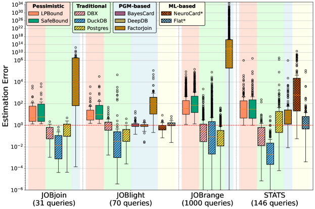
Figure 5: Estimation errors for JOBJoin, JOBLight, JOBRange, and STATS. For the starred ML-based estimators, we use the errors for JOBLight and STATS reported in the literature [15].

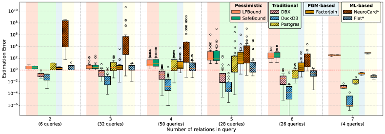
Figure 6: Estimation errors for STATS. For the starred ML-based estimators, we use errors reported in the literature [15].

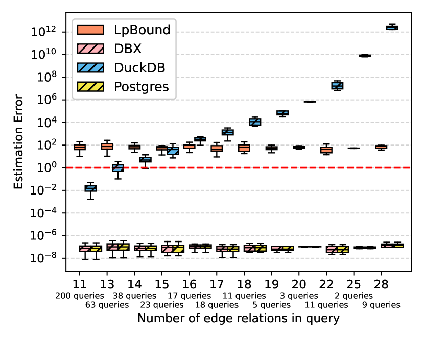
Figure 7: Estimation errors for the SM cyclic queries.

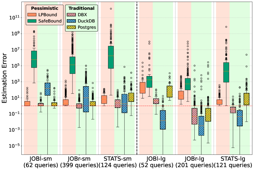
Figure 8: Estimation errors for group-by queries.

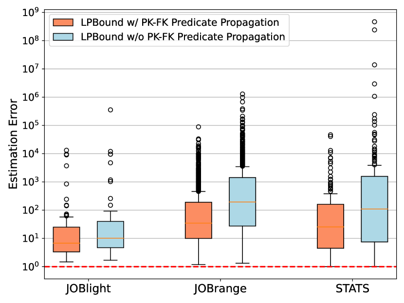
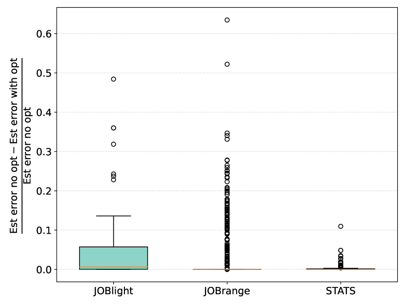
Figure 9: Improvements on estimation errors when using the two optimizations discussed in Sec. 5. Left: PK-FK predicate propagation optimization. Right: Prefix degree sequences optimization.

6.2 Estimation Errors

Acyclic queries.

LpBound has a smaller error range than the traditional estimators and SafeBound for acyclic queries. Fig. 5 plots the estimation errors for the acyclic queries. All systems except LpBound and SafeBound both underestimate and overestimate. The traditional estimators broadly use as estimation the multiplication of the relation sizes and of the selectivities of the query predicates. The selectivity of a join predicate is the inverse of the minimum of the domain sizes of the two join attributes (so average degree, as opposed to maximum degree, is used). For equality and range predicates, Most Common Values (for Postgres) and histograms (for Postgres and DbX) are used. DuckDB has a fixed selectivity of 0.2 for a range predicate. For ML-based estimators, we use the estimates reported in [15], as the models are not available. These models were designed to overfit JOBlight and subsequently fine-tuned to STATS, albeit with a poorer accuracy.

We also report on the estimation errors of the PGM-based estimators. BayesCard and DeepDB do very well on JOBlight; this is the only workload on which their implementation works. FactorJoin builds high-dimensional probability distributions over the attributes of each relation to capture their correlation. This building task uses random sampling for JOB and the more accurate BayesCard for STATS. FactorJoin faces a trade-off between good accuracy and fast estimation time. To keep the latter practical, it approximates the learned high-dimensional distributions by the product of one-dimensional distributions for JOB and of two-dimensional distributions for STATS. These choices influence the estimation error: It is far more accurate for STATS than for JOBjoin due to the choice of BayesCard over sampling and 2-dimensional over 1-dimensional factorization. The errors for JOBrange are larger possibly due to the larger number (up to 3) of predicates per relation.

Fig. 6 shows that the accuracy of the estimators decreases with the number of relations per query (shown for STATS, a similar trend also holds for JOBlight and JOBrange): The traditional estimators underestimate more, whereas the pessimistic estimators overestimate more. NeuroCard starts with a large overestimation for a join of two relations and decreases its estimation as we increase the number of relations; the other ML-based estimators follow this trend but at a smaller scale.

Cyclic queries.

LpBound is the most accurate estimator for the SM cyclic queries. Fig. 8 shows the errors of LpBound and the traditional estimators, grouped by the number of edge relations in the query. The learned estimators do not work for cyclic queries.

As we increase linearly the number $n$ of edge relations from 11 to 28, the number of join conditions between the edge relations increases quadratically in $n$. This poses difficulties to the traditional estimators, which exhibit two distinct behaviors.

The estimate of Postgres and DbX is 1 for all SM queries and their error is the inverse of the query output size. This is an underestimation by 7-8 orders of magnitude. The estimation is obtained by multiplying: the size of the edge relation $n$ times; the selectivity of each of the $n^{2}$ join conditions; the size of the vertex relation $2n$ times; the selectivity of the $2n$ join conditions between the edge and vertex relations; and the selectivity of the $2n$ equality predicates in the $2n$ vertex relations. The product of the relation sizes is much smaller than the inverse of the product of these selectivities, so the estimation is a number below 1, which is then rounded to 1.

The estimate of DuckDB increases exponentially in the number of edge relations, eventually leading to an overestimation by over 12 orders of magnitude. Its estimation ignores most of the join conditions, but accounts for each of the $n$ copies of the edge relation, as explained next. To estimate, DuckDB first constructs a graph, where each node is a relation in the query and there are two edges between any two nodes representing relations that are joined in the query: one edge per attribute participating in the join. Each edge is weighted by the inverse of the domain size of the attribute. DuckDB then takes a minimum-weight spanning tree of this graph. A significant factor in the estimation is then the multiplication of the ($n$ edge and $2n$ vertex) relation sizes at the nodes and of the weights of the edges in the spanning tree ($3n-1$ domain sizes of one or the other column in the edge or vertex relations). For each of the relations in the query, the estimate has thus a factor proportional to the fraction of the relation size over an attribute’s domain size.

Group-by queries.

The range of the estimation errors for group-by queries is the smallest for LpBound. Except for LpBound, Postgres, and DbX, the systems ignore the group-by clause and estimate the cardinality for the full query. Fig. 8 shows the errors for the small and large domain classes of JOBlight, JOBrange, and STATS group-by queries (the mixed domain class behaves very similarly to the large domain class). For small domain sizes (first half of figure), LpBound and Postgres use the product of the domain sizes, which is close to the true cardinalities. For large domain sizes (second half), the true cardinalities remain smaller than for the full queries, yet Postgres estimates are for the full queries. This explains why the error boxes are shifted up relative to those in Fig. 5. SafeBound and DuckDB estimate the full query and have large errors.

Optimization Improvements.

Fig. 9 shows the improvements to the estimation accuracy brought by each of the two optimizations discussed in Sec. 5, when taken in isolation.

The left figure shows that, when propagating predicates from the primary-key relation to the foreign-key relations, the estimation error can improve by over an order of magnitude in the worst case (corresponding to the upper dots in the plot) and by roughly 5x in the median case (corresponding to the red line in the boxplots).

The right figure shows that, when using prefix degree sequences for the degree sequences of relations without predicates, the estimation error can improve by up to 50% for JOBlight queries, up to 65% for JOBrange queries and up to 10% for STATS queries. The improvement is measured as the division of (i) the difference between the estimation error without this optimization and the estimation error with this optimization and (2) the the estimation error without this optimization.

Estimator	JOBjoin		JOBlight		STATS
	Time	Space	Time	Space	Time	Space
LpBound	0.48 / 10.5	0.04	0.36 / 1.5	1.25	0.49 / 1.6	3.62
SafeBound	0.85 / 147.9	0.07	1.28 / 13.0	1.75	1.89 / 5.6	5.94
DbX ${}^{\!+}$	- / 371.7	-	- / 35.3	-	- / 13.3	-
DuckDB ${}^{\!+}$	- / 99.4	-	- / 535.2	-	- / 30.3	-
Postgres ${}^{\!+}$	- / 19.8	$<$0.001	- / 3.4	0.001	- / 18.7	0.011
FactorJoin	0.66 / 202	31.6	16.7 / 166.5	22.8	35.3 / 626	8.2
BayesCard	- / -	-	3.0 / 21.7	1.6	- / -	-
DeepDB	- / -	-	4.3 / 28.6	34.0	- / -	-
NeuroCard ${}^{\!*}$	- / -	-	18.0 / -	6.9	23.0 / -	337.0
Flat ${}^{\!*}$	- / -	-	8.6 / -	3.4	175.0 / -	310.0

Table 2: Time (ms): average wall-clock times to compute estimates for (i) a sub-query of a query, averaged over all sub-queries of queries / (ii) a query and all its connected sub-queries, averaged over all queries. Space (MB): extra space for data statistics and models. The times (⁺) are for the entire query optimization task. The numbers (^∗) are from prior work [15] and only available for JOBlight and STATS. (-) means unavailable data or unsupported workload.

6.3 Estimation Times

LpBound has a very low estimation time (a few ms) thanks to its LP optimizations. At the other extreme, ML-based estimators can be 1-2 orders of magnitude slower even when taking their average estimation time per subquery instead of the estimation time for all subqueries.

To produce a plan for a query with $n$ relations, a query optimizer uses the cardinality estimates for some of the $k$-relation sub-queries for $2\leq k\leq n$. Following prior work [15, 32], we use the sub-queries produced by Postgres’s planner for a given query. The range (min-max) of the number of sub-queries is: 8-2018 for JOBjoin; 1-26 for JOBlight; and 1-75 for STATS. The times for JOBrange are not reported, but we expect them to be close to those for JOBlight. SM is not supported by the ML-based estimators and SafeBound.

We report two estimation times per benchmark: (i) the time to compute the estimate for a single sub-query, averaged over all sub-queries of all queries, and (ii) the time to compute the estimates for a query and all its sub-queries, averaged over all queries.

Table 2 reports the estimation times of the estimators. It was not possible to get the estimation times for the traditional estimators, so we report instead their times for the entire query optimization task to give a context for the other reported times; thy should have the lowest estimation times. The type (i) times for the starred ML-based estimators are from [15]. We expect their type (ii) times to be at least an order of magnitude larger than their type (i) times, given the average number of sub-queries per query.

FactorJoin computes the estimates for all sub-queries of a query in a bottom-up traversal of a left-deep query plan. This computation does not parallelize well, however. Its type (i) time is therefore much lower than the type (ii) time.

LpBound can effectively parallelize the LP solving for the sub-queries of a query. Even though one can extend an already constructed LP to accommodate new relations and statistics, we found that it is faster to avoid estimation dependencies between the related sub-queries and estimate for them independently in parallel.

6.4 Space Requirements

The extra space used by LpBound for statistics is 1.6x less than of SafeBound and 1.2-93x less than of the ML-based estimators.

Table 2 shows the amount of extra space needed to store the data statistics or machine learning models used by the estimators.

The traditional estimators use modest extra space. Postgres uses 100 MCVs per predicate column: Increasing the number of MCVs leads to very large estimation time, as it computes the join output size at estimation time for the MCVs. It also uses 100 buckets per histogram and sampling-based estimates of domain sizes for columns. DuckDB only uses (very accurate and computed using hyperloglog [11, 17]) domain size estimates, no MCVs, and no histograms. DbX uses histograms with 200 buckets and no MCVs.

SafeBound uses a compressed representation of the degree sequences and 2056 MCVs on the predicate columns.

LpBound uses up to 5000 MCVs on the predicate columns in JOB, albeit for less space than SafeBound. Both SafeBound and LpBound use hierarchical histograms on data columns with 128 buckets. LpBound stores $\ell_{p}$-norms within each histogram bucket, while SafeBound stores $\ell_{1}$-norms (counts) only. Although not reported in the table, LpBound needs 1.12MB for SM and 8MB for JOBrange. JOBrange has queries with more predicates, which need support, and more columns with large domains.

The models used by NeuroCard and Flat are a feature-rich representation of the datasets. They take more space than the statistics used by the other estimators. For STATS, these models take 10x more space than the dataset itself [15].

Estimator	JOBjoin	JOBlight	JOBrange	STATS	SM
LpBound-${\ell_{1}}$	4.07	12.35	42.42	24.67	0.65
LpBound	14.95	19.06	54.79	27.91	1.59
SafeBound	88.56	162.09	209.23	32.04	-
FactorJoin	10068.8	4990.9	5042.7	360.92	-
BayesCard	-	493.36	-	-	-
DeepDB	-	1191.17	-	-	-
NeuroCard ∗	-	3600	-	-	-
Flat ∗	-	3060	-	-	-

Table 3: Time (sec) to compute the required statistics for the pessimistic and PGM-based estimators. LpBound-${\ell_{1}}$ is LpBound with $\ell_{1}$-norms only. (-) means the system cannot estimate for the respective workload. (*) means the times are from prior work [15], as the code is not available.

6.5 Time to Compute the Statistics

Table 3 gives the times to compute the statistics or models required by the estimators. Overall, the compute time for LpBound is at least one order of magnitude smaller than for the PGM-based estimators. The computation of the statistics used by LpBound is fully expressed in SQL and executed using DuckDB. Such statistics are: the MCVs, the histograms, the $\ell_{p}$-norms ($p\in\{1,\ldots,10,\infty\}$) for each MCV, histogram bucket, and full relation, and the two optimizations (FKPK and prefix) from Sec. 5. About 80% of LpBound’s time is spent on the two optimizations. To better understand the effect of the number of norms, we also report the times for LpBound when restricted to the $\ell_{1}$-norm only. This shows that increasing from 1 to 11 norms only increases the compute time 1.5–3.7 times. DeepDB and BayesCard take 86% and respectively 67% of their compute time for training, the remaining time is for constructing an auxiliary data structure to support efficient sampling. FactorJoin spends most of its time (98%) to construct statistics to speed up the estimation, while relatively very short time (2%) is spent on training the model. The times for NeuroCard and Flat are as reported in prior work [15] for training without hyper-parameter tuning.

6.6 From Cardinality Estimates to Query Plans

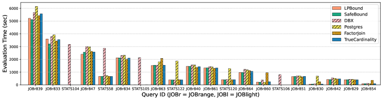
Figure 10: Postgres (wall-clock) evaluation time for the 20 most expensive queries in JOBlight, JOBrange, and STATS, when injected the estimates of LpBound, SafeBound, DbX, and Postgres or the trues cardinalities for all subqueries of the query. The runtimes for STATS 104, 105, 106 are very small when using the estimates of all systems but DbX and therefore not visible.

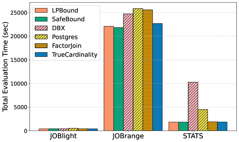
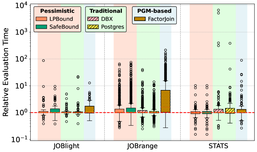
Figure 11: Left: Overall evaluation time of all queries in a benchmark for Postgres when using estimates for all subqueries from LpBound, SafeBound, DbX, Postgres and true cardinalities. Right: Relative evaluation times compared to the baseline evaluation time obtained when using true cardinalities.

When injected the estimates of LpBound, Postgres derives query plans at least as good as those derived using the true cardinalities.

This result was expected and aligns with observations from prior work [6, 10]. We verified this for the 20 queries in JOBlight, JOBranges, and STATS (Fig. 10), which took longest to execute using Postgres when the query plan was generated based on the estimations of LpBound, SafeBound, DbX, Postgres, or FactorJoin. We used Postgres for query execution as it easily allows to inject external estimates into its query optimizer. Remarkably, the estimates of LpBound can lead to better Postgres query plans than using true cardinalities, e.g., for the 9 most expensive JOBrange queries in the figure. Prior work [26] also reported this surprising behavior that using true cardinalities, Postgres does not necessarily pick better query plans. SafeBound leads to better plans than LpBound for the top-2 most expensive queries. The estimates of DbX and Postgres lead in many cases to much slower query plans: for STATS104 (STATS122), DbX (Postgres) estimates lead to a plan that is more than 3000x (4x) slower than for the other estimators. For three STATS queries (104, 105, 106), the DbX estimates yield a very slow plan; the runtimes of the plans using the estimates of the other systems are not visible in the plot.

Fig. 11 (left) shows the aggregated Postgres evaluation time of all queries in JOBlight, JOBrange, and STATS when using estimates for all sub-queries from LpBound, SafeBound, DbX, Postgres, and true cardinalities (left). Fig. 11 (right) shows the relative evaluation times compared to the baseline evaluation time obtained when using true cardinalities. We have two observations. First, overestimation can be beneficial for performance of expensive queries, which has been discussed in Section 6. Second, overestimation can be detrimental for performance of less expensive queries in some cases.

The first observation is reflected in the overall evaluation times, which are dominated by the most expensive queries in the benchmark (some of which are listed in Fig. 10). Traditional approaches lead to higher evaluation times for the expensive queries, and therefore to higher overall evaluation times, while the pessimistic approaches lead to lower evaluation times for those expensive queries. Overall, the evaluation times for the pessimistic approaches are about the same (JOBlight and STATS) or lower (JOBrange) than the baseline evaluation times. The second observation is reflected in the relative evaluation times for the JOB benchmarks. The boxplots for the traditional approaches are lower than those for the pessimistic approaches, indicating that the traditional approaches perform better for the less expensive queries in the benchmarks.

FactorJoin has both high overall evaluation time and high relative evaluation time. It estimates very accurately for the queries in STATS, thus has similar evaluation time to the baseline evaluation time. For the queries in JOBlight and JOBrange, it mostly overestimates, which leads to lower evaluation times for the expensive queries. However, the overestimations are significant, which makes it perform worse than the pessimistic approaches for the less expensive queries, as shown in the right plot of Fig. 11. This leads to the high overall evaluation time of FactorJoin.

6.7 Performance Considerations for LpBound

How Many $\ell_{p}$-Norms to keep?

Using the norms for $p\in[1,10]\cup\{\infty\}$ gives the best trade-off between the space requirements, the estimation error, and the estimation time for the JOBlight queries (Fig. 13). This was verified to hold also for the other benchmarks. Further norms can still lower the estimation error, but only marginally, and at the expense of more space and estimation time.

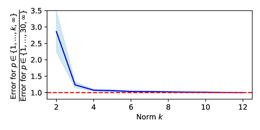
Figure 12: The amount of useful norms follows the law of diminishing returns: Plotting the division of estimation errors for the norms $\{1,\ldots,k,\infty\}$ and $\{1,\ldots,30,\infty\}$, averaged over the 70 JOBlight queries.

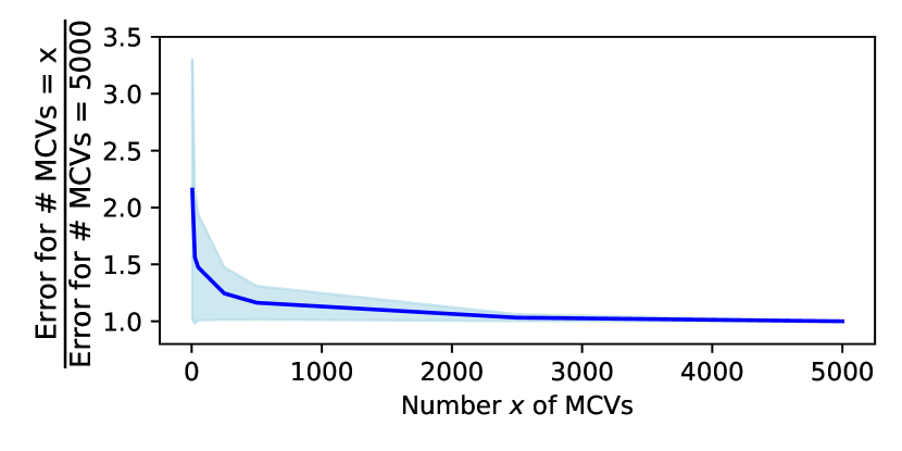
Figure 13: Effect of the number of MCVs on estimation error for LpBound on JOBlight.

How many Most Common Values (MCVs)?

Using sufficiently many MCVs to support the estimation for selection predicates can effectively reduce the overall estimation error. For each of the top-$k$ MCVs of a predicate attribute, LpBound stores one set of $\ell_{p}$-norms. It also stores one further set of norms for all remaining attribute values (Sec. 5). For small-domain attributes, e.g., COMPANY_TYPE, it is often feasible to have MCVs for each domain value. This significantly improves the estimation accuracy. For large-domain attributes, e.g., COMPANY_ID, it not not practical to do so. To decide on the number $k$ of MCVs, one can plot the estimation error as a function of $k$ and pick $k$ so that the improvement in estimation error for larger $k$ is below a threshold, e.g., $1\%$. Fig. 13 shows that $k\leq 2500$ can yield on average to clear accuracy improvements for JOBlight; this is similar for JOBrange (not shown).

Optimizations for LpBound’s LPs.

The optimizations introduced for solving LpBound’s LPs are essential for the practicality of LpBound. Fig. 14 shows the estimation time of LpBound using $\texttt{LP}_{\text{base}}$, $\texttt{LP}_{\text{flow}}$, and $\texttt{LP}_{\text{Berge}}$. We used JOBjoin, as its queries are Berge-acyclic and have the largest number of relations and variables among the considered benchmarks, and therefore can stress test and compare the efficiency of the three approaches. As expected, $\texttt{LP}_{\text{base}}$ takes too long (over 1000 seconds) to build and solve an LP with $2^{15}$ entropic terms and times out beyond this. $\texttt{LP}_{\text{flow}}$ uses a network flow of size at most $15^{2}$ and finishes in under 70 ms for each JOBjoin query. Most of its time is spent constructing the network. $\texttt{LP}_{\text{Berge}}$ consistently takes under 2ms for all queries.

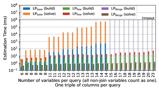
Figure 14: Estimation times for LpBound on full queries of JOBjoin using $\texttt{LP}_{\text{base}}$ and its optimizations $\texttt{LP}_{\text{flow}}$ and $\texttt{LP}_{\text{Berge}}$.

7 Conclusion and Future Work

In this paper we introduced LpBound, a pessimistic cardinality estimator that uses $\ell_{p}$-norms of degree sequences of the join columns and information inequalities. The advantages of LpBound over the learned estimators such as FactorJoin, BayesCard, and DeepDB, NeuroCard, and Flat are that it provides: strong, one-sided theoretical guarantees; low estimation time and error when applied to workloads not seen before; fast construction of the necessary statistics; and a rich query language support with (cyclic and acyclic) equality joins, equality and range predicates, and group-by variables. This language support goes significantly beyond the star or even acyclic queries supported by the competing estimators benchmarked in Section 6.

While LpBound’s estimation time is slightly larger than that of traditional estimators, it can nevertheless have lower estimation errors and lead to significantly improved query performance: Fig. 10 shows that the runtime improvement can be up to 3000 seconds for some queries, while its estimation time is only a few milliseconds.

There are two major limitations of LpBound, as introduced in this paper. First, it can non-trivially overestimate the cardinality of joins of highly miscalibrated relations. We introduced two optimizations in Sec. 5 to mitigate this problem. Second, it does not yet support range (and theta) joins, complex and negated predicates, and nested queries. LpBound’s flexible framework can in principle accommodate such query constructs, yet this is not immediate and deserves an in-depth treatment in future work. For example, an arbitrary predicate could be accommodated using appropriate data structures that can identify the ranges of tuples that satisfy the predicate and that can be adjusted to store norms on the degree sequences within such ranges. A LIKE predicate can be accommodated, for instance, using a 3-gram index to select ranges of tuples that satisfy the predicate, similar to SafeBound [10]. To guarantee that LpBound returns an upper bound on the true cardinality of the query, the returned ranges must include all matching tuples.

To support nested queries, LpBound needs to become compositional, i.e., to take $\ell_{p}$-norms on input relations and return upper bounds on $\ell_{p}$-norms on the query output. Given a nested query $Q$, LpBound needs to first compute upper bounds on $\ell_{p}$-norms on the relations representing the sub-queries of $Q$ and then use these bounds to estimate the cardinality of $Q$.

Future work also needs to address the efficient maintenance of LpBound’s estimation under data updates. The following three observations outline a practical approach to achieve this. First, the q-inequality $|Q|\leq\prod\left(||\texttt{deg}_{R}(V|U)||_{p}\right)^{w^{*}}$, where the product ranges over all available statistics constraints, holds with the same weights $w^{*}$ even when the norms $||\texttt{deg}_{R}(V|U)||_{p}$ change. This means that we do not need to solve the LP after every data update to obtain a valid upper bound on the cardinality of a query $Q$. Second, the $\ell_{p}$-norms used by LpBound can be expressed in SQL (as for Experiment 6.5) and maintained efficiently under data updates using the view maintenance mechanism of the underlying database system, e.g., delta queries. Third, we envision the use of $\ell_{p}$-sketches [8] for an efficient, albeit approximate, maintenance of the $\ell_{p}$-norms.

Appendix A Supplementary Material

This is extra material for the submission titled "LpBound: Pessimistic Cardinality Estimation Using $\ell_{p}$-Norms of Degree Sequences." This material is organized as follows. Section A.1 gives the proof for Theorem 4.1. Section A.2 describes a third optimized algorithm for estimating arbitrary conjunctive queries, which uses hypertree decompositions of the queries. This is not yet implemented in LpBound. Section A.3 gives more details on the $\texttt{LP}_{\text{flow}}$ optimization and the proof for Theorem 4.5.

A.1 Proof of Theorem 4.1

For simplicity of presentation, we assume here that the query $Q$ is connected. Denote by $b_{\text{base}}$ and $b_{\text{Berge}}$ the values of $\texttt{LP}_{\text{base}}$ and $\texttt{LP}_{\text{Berge}}$. The inequality $b_{\text{base}}\leq b_{\text{Berge}}$ follows from two observations:

• For any acyclic query $Q$ and any polymatroid $h$, the inequality $E_{Q}\geq h(X_{1}\cdots X_{n})$ is a Shannon inequality. This is a well known inequality [24, 21] (which we review in Lemma A.6 below).

• Any feasible solution to $\texttt{LP}_{\text{base}}$ can be converted to a feasible solution of $\texttt{LP}_{\text{Berge}}$ by simply “forgetting” the terms $h(U)$ that do not occur in $\texttt{LP}_{\text{Berge}}$.

For the converse, $b_{\text{Berge}}\leq b_{\text{base}}$, we will prove that every feasible solution $h$ to $\texttt{LP}_{\text{Berge}}$ can be extended to a feasible solution to $\texttt{LP}_{\text{base}}$ (by defining $h(U)$ for all terms $h(U)$ that did not appear in $\texttt{LP}_{\text{Berge}}$), such that $E_{Q}=h(X_{1}\cdots X_{n})$. We will actually prove something stronger: that $h$ can be extended to a normal polymatroid.

Definition A.1.

A set function $h:2^{\{X_{1},\ldots,X_{n}\}}\rightarrow\mathbb{R}$ is a normal polymatroid if $h(\emptyset)=0$ and it satisfies:

$$\forall U\subseteq\{X_{1},\ldots,X_{n}\}:\sum_{W\subseteq U}(-1)^{|W|+1}h(W)\geq 0$$ (24)

It is known that every normal polymatroid is an entropic vector, and every entropic vector is a polymatroid, but none of the converse holds.

The inequality $b_{\text{Berge}}\leq b_{\text{base}}$ follows from two lemmas:

Lemma A.2.

Let $V=\{X_{1},\ldots,X_{n}\}$, let $a_{1},\ldots,a_{n},A$ be $n+1$ non-negative numbers such that:

$$a_{1}+\cdots+a_{n}\geq A\ \ \ \ \text{and}\ \ \ \ \ a_{i}\leq A,\forall i=1,n$$ (25)

Then there exists a normal polymatroid $h:2^{V}\rightarrow\mathbb{R}$ such that $h(X_{i})=a_{i}$ for all $i=1,n$ and $h(V)=A$.

Lemma A.3 (Stitching Lemma).

Let $V_{1},V_{2}$ be two sets of variables, $Z\stackrel{{\scriptstyle\text{def}}}{{=}}V_{1}\cap V_{2}$. Let $h_{1}:2^{V_{1}}\rightarrow\mathbb{R}$, $h_{2}:2^{V_{2}}\rightarrow\mathbb{R}$ be two normal polymatroids that agree on their common variables $Z$: in other words there exists $h:2^{Z}\rightarrow\mathbb{R}$ such that $\forall U\subseteq Z$, $h_{1}(U)=h(U)=h_{2}(U)$. Define the following function $h^{\prime}:2^{V_{1}\cup V_{2}}\rightarrow\mathbb{R}$:

$$h^{\prime}(U)\stackrel{{\scriptstyle\text{def}}}{{=}} h_{1}(U\cap V_{1}|U\cap Z)+h_{2}(U\cap V_{2}|U\cap Z)+h(U\cap Z)$$ (26)

Then $h^{\prime}$ is a normal polymatroid that agrees with $h_{1}$ on $V_{1}$ and with $h_{2}$ on $V_{2}$, and, furthermore, satisfies:

$$h^{\prime}(V_{1}\cup V_{2})= h^{\prime}(V_{1})+h^{\prime}(V_{2})-h^{\prime}(V_{1}\cap V_{2})$$ (27)

In essence, this says that $V_{1},V_{2}$ are independent conditioned on $V_{1}\cap V_{2}$.

Notice that $h^{\prime}$ can be written equivalently as $h^{\prime}(U)=h_{1}(U\cap V_{1})+h_{2}(U\cap V_{2})-h(U\cap Z)$. While each term is a normal polymatroid, it is not obvious that $h^{\prime}$ is too, because of the difference operation. In fact, if $h_{1},h_{2},h$ are polymatroids, then $h^{\prime}$ is not a polymatroid in general.

The two lemmas prove Theorem 4.1, by showing that $b_{\text{Berge}}\leq b_{\text{base}}$, as follows. Consider any feasible solution $h$ to $\texttt{LP}_{\text{Berge}}$. Consider first a single atom $R_{j}(V_{j})$ of $Q$: $h$ is only defined on all its variables and on the entire set $V_{j}$. By Lemma A.2, we can extend $h$ to a normal polymatroid $h:2^{V_{j}}\rightarrow{\mathbb{R}}_{\tiny+}$. We do this separately for each $j=1,m$. Next, we stitch these polymatroids together in order to construct a polymatroid on all variables, $h:2^{\{X_{1},\ldots,X_{n}\}}\rightarrow{\mathbb{R}}_{\tiny+}$, and for this purpose we use the Stitching Lemma A.3. Notice that the Lemma is stronger than what we need, since in our case the intersection $V_{1}\cap V_{2}$ always has size 1 (since $Q$ is Berge-acyclic): we need the stronger version for our third algorithm described in Sec. A.2. By using the conditional independence equality (27), we can prove that $E_{Q}=h(X_{1}\cdots X_{n})$, which completes the proof of Theorem 4.1.

It remains to prove the two lemmas.

Proof of Lemma A.2.

We briefly review an alternative definition of normal polymatroids from [30]. For any $U\subseteq V$, the step function at $U$ is $h^{U}$ defined as:

$$\forall X\subseteq V: h^{U}(X)\stackrel{{\scriptstyle\text{def}}}{{=}} \begin{cases}1&\mbox{if $U\cap X\neq\emptyset$}\\ 0&\mbox{otherwise}\end{cases}$$ (28)

When $U=\emptyset$, then $h^{U}\equiv 0$, so we will assume w.l.o.g. that $U\neq\emptyset$. A function $h:2^{V}\rightarrow\mathbb{R}$ is a normal polymatroid iff it is a non-negative linear combination of step functions:

$$h= \sum_{U\subseteq V,U\neq\emptyset}c_{U}h^{U}$$ (29)

where $c_{U}\geq 0$ for all $U$.

We prove the lemma by induction on $n$, the number of variables in $V$. If $n=1$ then the lemma holds trivially because we define $h(X_{1})\stackrel{{\scriptstyle\text{def}}}{{=}}a_{1}$, so assume $n\geq 2$. Rename variables such that $a_{1}\geq a_{2}\geq\cdots\geq a_{n}$, and let $k\leq n$ be the smallest number such that $a_{1}+\cdots+a_{k}\geq A$: such $k$ must exist by assumption of the lemma. We prove the lemma in two cases.

Case 1: $k=n$. Let $\delta\stackrel{{\scriptstyle\text{def}}}{{=}}\sum_{i=1,n}a_{i}-A$ be the excess of the inequality (25): notice that $a_{1}\geq\delta$ and $a_{n}\geq\delta$. We define $h$ as follows:

$$h= (a_{1}-\delta)h^{X_{1}}+\delta h^{X_{1},X_{n}}+\sum_{i=2,n-1}a_{i}h^{X_{i}}+(a_{n}-\delta)h^{X_{n}}$$

By construction, $h$ is a normal polymatroid, and one can check by direct calculation that $h(X_{i})=a_{i}$ for all $i$ and $h(V)=A$.

Case 2: $k<n$. We prove by induction on $m=k,k+1,\ldots,n$ that there exists a normal polymatroid $h:2^{\{X_{1},\ldots,X_{m}\}}\rightarrow\mathbb{R}$ s.t. $h(X_{i})=a_{i}$ for $i=1,m$ and $h(X_{1}\ldots X_{m})=A$. The claim holds for $m=k$ by Case 1. Assuming it holds for $m-1$, let $h^{\prime}:2^{\{X_{1},\ldots,X_{m-1}\}}\rightarrow\mathbb{R}$ be such that $h^{\prime}(X_{i})=a_{i}$ for $i=1,m-1$ and $h^{\prime}(X_{1}\cdots X_{m-1})=A$. We show that we can extend it to $X_{m}$. For that we first represent $h^{\prime}$ over the basis of step functions:

$$h^{\prime}= \sum_{U\subseteq\{X_{1},\ldots,X_{m-1}\},U\neq\emptyset}c_{U}h^{U}$$

for some coefficients $c_{U}\geq 0$, and note that $\sum_{U}c_{U}=h^{\prime}(X_{1}\ldots X_{m-1})=A$. Define $h$ as follows:

$$h= \sum_{U\subseteq\{X_{1},\ldots,X_{m-1}\},U\neq\emptyset}c_{U}\left(1-\frac{a_{m}}{A}\right)h^{U}+\sum_{U\subseteq\{X_{1},\ldots,X_{m-1}\},U\neq\emptyset}c_{U}\frac{a_{m}}{A}h^{U\cup\{X_{m}\}}$$

By assumption of the lemma $a_{m}\leq A$, which implies that all coefficients above are $\geq 0$, hence $h$ is a normal polymatroid. Furthermore, by direct calculations we check that, for $i<m$, $h(X_{i})=h^{\prime}(X_{i})=a_{i}$ (because $h^{U\cup\{X_{m}\}}(X_{i})=h^{U}(X_{i})$), and, for $i<m$, $h(X_{m})=a_{m}$, because $h^{U}(X_{m})=0$ and $h^{U\cup\{X_{m}\}}(X_{m})=1$, and the claim follows from $\sum_{U}c_{U}=h^{\prime}(X_{1}\cdots X_{m-1})=A$. Finally, we also have $h(X_{1}\ldots X_{m})=\sum_{U}c_{U}=A$, as required. ∎

Finally, we prove the Stitching Lemma A.3. For that we need two propositions.

Proposition A.4.

Let $h:2^{V}\rightarrow\mathbb{R}$ be a normal polymatroid, and $V_{0}\supseteq V$ a superset of variables. Define $h^{\prime}:2^{V_{0}}\rightarrow\mathbb{R}$ by $h^{\prime}(U)\stackrel{{\scriptstyle\text{def}}}{{=}}h(U\cap V)$ for all $U\subseteq V_{0}$. Then $h^{\prime}$ is a normal polymatroid. In other words, $h^{\prime}$ extends $h$ to $V_{0}$ by simply ignoring the additional variables.

Proof.

We verify condition (24) directly. When $U\subseteq V$, then $h^{\prime}(W)=h(W)$ for all $W\subseteq U$ and the condition holds because $h$ is a normal polymatroid. When $U\not\subseteq V$, then we claim that $\sum_{W\subseteq U}(-1)^{|W|+1}h(W\cap V)=0$. Indeed, fix a variable $X_{i}\in U$, $X_{i}\not\in V$, and pair every subset $W\subseteq U$ that does not contain $X_{i}$ with $W^{\prime}\stackrel{{\scriptstyle\text{def}}}{{=}}W\cup\{X_{i}\}$. Then $h(W\cap V)=h(W^{\prime}\cap V)$ and the two terms corresponding to $W$ and $W^{\prime}$ in (24) cancel out, proving that the expression (24) is $=0$. ∎

Proposition A.5.

Let $h:2^{V}\rightarrow\mathbb{R}$ be a normal polymatroid, and $Z\subseteq V$ a subset of variables. Define the following set functions $h^{\prime},h^{\prime\prime}:2^{V}\rightarrow\mathbb{R}$:

$$\forall U\subseteq V: h^{\prime}(U)\stackrel{{\scriptstyle\text{def}}}{{=}} h(U\cap Z) h^{\prime\prime}(U)\stackrel{{\scriptstyle\text{def}}}{{=}} h(U|U\cap Z)$$ (30)

(Recall that $h(B|A)=h(AB)-h(A)$.) Then both $h^{\prime},h^{\prime\prime}$ are normal polymatroids.

Proof.

We consider two cases as above. When $U\subseteq Z$, then for all $W\subseteq U$ we have $h^{\prime}(W)=h(W)$, and $h^{\prime\prime}(W)=0$: condition (24) holds for $h^{\prime}$ because it holds for $h$, and it holds for $h^{\prime\prime}$ trivially since it is $=0$. No consider $U\not\subseteq Z$. Then we claim that the expression (24) for $h^{\prime}$ is $0$:

$$\sum_{W\subseteq U}(-1)^{|W|+1}h^{\prime}(W)= \sum_{W\subseteq U}(-1)^{|W|+1}h(W\cap Z)=0$$

We use the same argument as in the previous lemma: pick a variable $X_{i}$ s.t. $X_{i}\in U$ and $X_{i}\not\in Z$ and pair each set $W\subseteq U$ that does not contain $X_{i}$ with the set $W^{\prime}\stackrel{{\scriptstyle\text{def}}}{{=}}W\cup\{X_{i}\}$. Then $h(W\cap Z)=h(W^{\prime}\cap Z)$ and two terms for $W$ and $W^{\prime}$ cancel out. Finally, condition (24) for $h^{\prime\prime}$ follows similarly:

$$\sum_{W\subseteq U}(-1)^{|W|+1}h^{\prime\prime}(W)= \sum_{W\subseteq U}(-1)^{|W|+1}h(W|W\cap Z)=\underbrace{\sum_{W\subseteq U}(-1)^{|W|+1}h(W)}_{\geq 0}-\underbrace{\sum_{W\subseteq U}(-1)^{|W|+1}h(W\cap Z)}_{=0}$$ (31)

The first term is $\geq 0$ because $h$ is a normal polymatroid, and the second term is $=0$, as we have seen. ∎

Finally, we prove the Stitching Lemma A.3.

Proof of Lemma A.3.

We first use the two propositions to show that $h^{\prime}$ from Eq. (26) is a normal polymatroid. Define two helper functions $h^{\prime}_{1}:2^{V_{1}}\rightarrow\mathbb{R}$ and $h^{\prime}_{2}:2^{V_{2}}\rightarrow\mathbb{R}$:

$$\forall U\subseteq V_{1}:\ h^{\prime}_{1}(U)\stackrel{{\scriptstyle\text{def}}}{{=}} h_{1}(U|U\cap Z) \forall U\subseteq V_{2}:\ h^{\prime}_{2}(U)\stackrel{{\scriptstyle\text{def}}}{{=}} h_{2}(U|U\cap Z)$$

By Lemma A.5, both $h^{\prime}_{1},h^{\prime}_{2}$ are normal polymatroids. Next, we extend $h^{\prime}_{1},h^{\prime}_{2},h$ to the entire set $V_{1}\cup V_{2}$ by defining:

$$\forall U\subseteq V_{1}\cup V_{2}: h^{\prime\prime}_{1}(U)\stackrel{{\scriptstyle\text{def}}}{{=}} h^{\prime}_{1}(U\cap V_{1}) h^{\prime\prime}_{2}(U)\stackrel{{\scriptstyle\text{def}}}{{=}} h^{\prime}_{2}(U\cap V_{2}) h^{\prime\prime}(U)\stackrel{{\scriptstyle\text{def}}}{{=}} h(U\cap Z)$$

By Lemma A.4 each of them is a normal polymatroid. Since $h^{\prime}$ in the corollary is their sum, it is also a normal polymatroid.

We check that it agrees with $h_{1}$ on $V_{1}$. For any $U\subseteq V_{1}$, we have $h_{2}(U\cap V_{2}|U\cap Z)=0$ therefore:

$$h^{\prime}(U)= h_{1}(U\cap V_{1}|U\cap Z)+h(U\cap Z)=h_{1}(U|U\cap Z)+h_{1}(U\cap Z)=h_{1}(U)$$

Similarly, $h^{\prime}$ agrees with $h_{2}$ on $V_{2}$. Finally, condition (27) follows by setting $U:=V_{1}\cup V_{2}$ in (26) and applying the definition of conditional: $h(B|A)=h(B)-h(A)$ when $A\subseteq B$. ∎

A.2 $\texttt{LP}_{\text{TD}}$: Using Hypertree Decomposition

The $\texttt{LP}_{\text{Berge}}$ algorithm is strictly limited by two requirements: $Q$ needs to be Berge-acyclic, and all statistics need to be full. We describe here a generalization of $\texttt{LP}_{\text{Berge}}$, called $\texttt{LP}_{\text{TD}}$, which drops these two limitations. When the restrictions of $\texttt{LP}_{\text{Berge}}$ are met, then $\texttt{LP}_{\text{TD}}$ is slightly less efficient, however, its advantage is that it can work on any query and constraints, without any restrictions.

A Hypertree Decomposition of a full conjunctive query $Q$ is a pair $(T,\chi)$, where $T$ is a tree and $\chi:\text{Nodes}(T)\rightarrow 2^{V}$ satisfying the following:

• For every variable $X_{i}$, the set $\{{t\in\text{Nodes}(T)}\mid{X_{i}\in\chi(t)}\}$ is connected. This is called the running intersection property.

• For every atom $R_{j}(V_{j})$ of $Q$, $\exists t\in\text{Nodes}(T)$ s.t. $V_{j}\subseteq\chi(t)$.

Each set $\chi(t)\subseteq V$ is called a bag. The width of the tree $T$ is defined as $w(T)\stackrel{{\scriptstyle\text{def}}}{{=}}\max_{t\in\text{Nodes}(T)}|\chi(t)|$. We review a lemma by Lee [24]:

Lemma A.6.

[24] Let $(T,\chi:\text{Nodes}(T)\rightarrow 2^{V})$ have the running intersection property and let $h:2^{V}\rightarrow\mathbb{R}$ be a set function. Define:

$$E_{T,h}\stackrel{{\scriptstyle\text{def}}}{{=}} \sum_{t\in\text{Nodes}(T)}h(\chi(t))-\sum_{(t_{1},t_{2})\in\text{Edges}(T)}h(\chi(t_{1})\cap\chi(t_{2}))$$ (32)

(1) If $h$ is a polymatroid (i.e. it satisfies the basic Shannon inequalities), then $E_{T,h}\geq h(V)$. (2) Suppose $h$ is the entropic vector defined by a uniform probability distribution on a relation $R(X_{1},\ldots,X_{n})$. Then, $E_{T,h}=h(V)$ if for every $(t_{1},t_{2})\in\text{Edges}(T)$, the join dependency $R=\Pi_{V_{1}}(R)\Join\Pi_{V_{2}}(R)$ holds, where $V_{1},V_{2}\subseteq V$ are the variables occurring on the two connected components of $T$ obtained by removing the edge $(t_{1},t_{2})$.

For a simple illustration, consider the 3-way join $J_{3}$ (Eq. (2)). Its tree decomposition $T$ has 3 bags $XY,YZ,ZU$, and $E_{T,h}=h(XY)+h(YZ)+h(ZU)-h(Y)-h(Z)$; one can check that $E_{T,h}\geq h(XYZU)$ using two applications of submodularity.

Our new linear program, called $\texttt{LP}_{\text{TD}}$, is constructed from a hypertree decomposition $(T,\chi)$ of the query as follows:

The Real-valued Variables are all expressions of the form $h(U)$ for $U\subseteq\chi(t)$, $t\in\text{Nodes}(T)$. The total number of real-valued variable is $\sum_{t\in\text{Nodes}(T)}2^{|\chi(t)|}$, i.e. it is exponential in the tree-width of the query.

The Objective is to maximize $E_{T,h}$ (Eq. (32)), subject to the following constraints.

Statistics Constraints: All statistics constraints Eq. (18) of $\texttt{LP}_{\text{base}}$. Since we don’t have numerical variable $h(U)$ for all $U$, we must check that (18) uses only available numerical variables. This holds, because each statistics refers to some atom $R_{j}(V_{j})$, and there exists of some bag such that $V_{j}\subseteq\chi(t)$, therefore we have numerical variables $h(U)$ for all $U\subseteq V_{j}$.

Normality Constraints: For each bag $\chi(t)$, $\texttt{LP}_{\text{TD}}$ contains all constraints of the form (24). In other words, the restriction of $h$ to $\chi(t)$ is normal.

We prove:

Theorem A.7.

$\texttt{LP}_{\text{base}}$ and $\texttt{LP}_{\text{TD}}$ compute the same value.

The theorem holds only when all degree constraints used in the statistics are simple, as we assumed throughout this paper. For a simple illustration, the $\texttt{LP}_{\text{TD}}$ for $J_{3}$ consists of 7 numerical variables
$h(X),h(Y),h(Z),h(U),h(XY),h(YZ),h(ZU)$ (we omit $h(\emptyset)=0$) and the following Normality Constraints:

$$h(X)+h(Y)-h(XY)\geq 0 h(Y)+h(Z)-h(YZ)\geq 0$$

$$h(Z)+h(U)-h(ZU)\geq 0$$

To compare $\texttt{LP}_{\text{TD}}$ and $\texttt{LP}_{\text{Berge}}$, assume that the query $Q$ is Berge-acyclic and all statistics are on simple and full degree constraints. The difference is that, for each atom $R_{j}(V_{j})$, $\texttt{LP}_{\text{Berge}}$ has only $1+|V_{j}|$ real-valued variables and only $1+|V_{j}|$ additivity constraints, while $\texttt{LP}_{\text{Berge}}$ has $2^{|V_{j}|}$ variables and normality constraints.

In the remainder of this section we prove Theorem A.7.

Denote by $b_{\text{base}}$ and $b_{\text{td}}$ the optimal solutions of $\texttt{LP}_{\text{base}}$ and $\texttt{LP}_{\text{TD}}$ respectively. We will prove that $b_{\text{base}}=b_{\text{td}}$.

First, we claim that $b_{\text{base}}\leq b_{\text{td}}$. It is known from [1] that $\texttt{LP}_{\text{base}}$ has an optimal solution $h^{*}$ that is a normal polymatroid; thus $b_{\text{base}}=h^{*}(V)$ (recall that $V$ is the set of all variables), where $h^{*}$ is normal. Then $h^{*}$ is also a feasible solution to $\texttt{LP}_{\text{TD}}$, therefore its optimal value is at least as large as the value given by $h^{*}$, in other words $b_{\text{td}}\geq E_{T,h^{*}}$. By Lemma A.6, we have $E_{T,h^{*}}\geq h^{*}(V)=b_{\text{base}}$, which proves the claim.

Second, we prove that $b_{\text{td}}\leq b_{\text{base}}$ by using the Stitching Lemma A.3. Let $h^{*}$ be an optimal solution to $\texttt{LP}_{\text{TD}}$, thus $b_{\text{td}}=E_{T,h^{*}}$. The function $h^{*}$ is defined only on subsets of the bags $\chi(t)$, $t\in\text{Nodes}(T)$, and on each such subset, it is a normal polymatroid. We extend it to a normal polymatroid defined on all variables $V=\bigcup_{t\in\text{Nodes}(T)}\chi(t)$ by repeatedly applying the Stitching Lemma A.3. Condition (27) of the corollary implies that this extension satisfies $h^{*}(V)=E_{T,h^{*}}$. Thus, $h^{*}$ is a normal polymatroid, and, hence, a feasible solution to $\texttt{LP}_{\text{base}}$. It follows that the optimal value of $\texttt{LP}_{\text{base}}$ is at least as large as that given by $h^{*}$, in other words $b_{\text{base}}\geq h^{*}(V)$. This completes the proof of the claim.

A.3 $\texttt{LP}_{\text{flow}}$: Missing Details from Section 4.2

Section 4.2 gives the high-level idea of the $\texttt{LP}_{\text{flow}}$ algorithm using an example. We give here a more formal description of the algorithm and prove Theorem 4.5. The input to $\texttt{LP}_{\text{flow}}$ is an arbitrary conjunctive query $Q$ of the form Eq. (1) (not necessarily a full query) and a set of statistics on the input database consisting of $\ell_{p}$-norms of simple degree sequences, i.e. statistics of the form $||\texttt{deg}_{R_{j}}(V|U)||_{p}$ where $|U|\leq 1$. For the purpose of describing $\texttt{LP}_{\text{flow}}$, we construct a flow network $G=(\text{Nodes},\text{Edges})$ that is defined as follows: (Recall that $\texttt{Vars}(Q)=\{X_{1},\ldots,X_{n}\}$ is the set of variables of the query.)

• The set of nodes $\text{Nodes}\subseteq 2^{\texttt{Vars}(Q)}$ consists of the following nodes:

  • The node $\emptyset$, which is the source node of the flow network.

  • A node $\{X_{i}\}$ for every variable $X_{i}\in\texttt{Vars}(Q)$.

  • A node $UV$ for every statistics $||\texttt{deg}_{R_{j}}(V|U)||_{p}$.

• The set of edges Edges consists of two types of edges:

  • Forward edges: These are edges of the form $(a,b)$ where $a,b\in\text{Nodes}$ and $a\subset b$. Each such edge $(a,b)$ has a finite capacity $c_{a,b}$. In particular, for every statistics $||\texttt{deg}_{R_{j}}(V|U)||_{p}$, we have two forward edges: One edge $(\emptyset,U)$ and another $(U,UV)$. (Recall that $|U|\leq 1$.)

  • Backward edges: These are edges of the form $(a,b)$ where $a,b\in\text{Nodes}$ and $b\subset a$. Each such edge $(a,b)$ has an infinite capacity $\infty$. In particular, for every statistics $||\texttt{deg}_{R_{j}}(V|U)||_{p}$ and every variable $X_{i}\in UV$, we have a backward edge $(UV,\{X_{i}\})$.

We are now ready to describe the linear program for $\texttt{LP}_{\text{flow}}$. Recall that $V_{0}$ is the set of group-by variables in the query $Q$ from Eq. (1).

The Real-valued Variables are of two types:

• Every statistics $||\texttt{deg}_{R_{j}}(V|U)||_{p}$ has an associated non-negative variable $w_{U,V,p}$.

• For every group-by variable $X_{i}\in V_{0}$, we have a flow variable $f_{a,b;X_{i}}$ for every edge $(a,b)\in\text{Edges}$.

The Objective is to minimize the following sum over all available statistics $||\texttt{deg}_{R_{j}}(V|U)||_{p}$:

$$\sum w_{U,V,p}\cdot\log||\texttt{deg}_{R_{j}}(V|U)||_{p}$$ (33)

The Constraints are of two types:

• Flow conservation constraints: For every group-by variable $X_{i}\in V_{0}$, the variables $f_{a,b;X_{i}}$ must define a valid flow from the source node $\emptyset$ to the sink node $\{X_{i}\}$ that has a capacity $\geq 1$. This means that for every node $c\in\text{Nodes}-\{\emptyset\}$, we must have:

  $$\sum_{a}f_{a,c;X_{i}}-\sum_{b}f_{c,b;X_{i}}\geq 1, c=\{X_{i}\}$$ if (34)

  $$\sum_{a}f_{a,c;X_{i}}-\sum_{b}f_{c,b;X_{i}}\geq 0,$$ otherwise (35)

• Flow capacity constraints: For every group-by variable $X_{i}\in V_{0}$ and every forward edge $(a,b)$, the flow variable $f_{a,b;X_{i}}$ must satisfy:

  $$f_{a,b;X_{i}}\leq c_{a,b}$$ (36)

  where $c_{a,b}$ is the capacity of the forward edge $(a,b)$. (Recall that backward edges have infinite capacity.) The capacity variables $c_{a,b}$ are determined by the statistics constraints. In particular, every statistics $||\texttt{deg}_{R_{j}}(V|U)||_{p}$ contributes a capacity of $w_{U,V,p}$ to $c_{U,UV}$ and a capacity of $\frac{w_{U,V,p}}{p}$ to $c_{\emptyset,U}$. Formally,

  $$c_{\emptyset,U} \stackrel{{\scriptstyle\text{def}}}{{=}}\sum_{p}w_{\emptyset,U,p}+\sum_{V,p}\frac{w_{U,V,p}}{p}$$ (37)

  $$c_{U,UV} \stackrel{{\scriptstyle\text{def}}}{{=}}\sum_{p}w_{U,V,p} U\neq\emptyset$$ if

We are now ready to prove Theorem 4.5, which says that the linear programs for $\texttt{LP}_{\text{base}}$ and $\texttt{LP}_{\text{flow}}$ have the same optimal value. To that end, we first write the dual LP for $\texttt{LP}_{\text{base}}$. For every statistics constraint of the form Eq. (18), we introduce a dual variable $w_{U,V,p}$. The dual of $\texttt{LP}_{\text{base}}$ is equivalent to:

$$\min\quad \sum w_{U,V,p}\cdot\log||\texttt{deg}_{R}(V|U)||_{p}$$ (38)

s.t. The following is a valid Shannon inequality:

$$h(V_{0})\leq\sum w_{U,V,p}\left(\frac{1}{p}h(U)+h(V|U)\right)$$ (39)

$$w_{U,V,p}\geq 0$$

Inequality (39) satisfies the property that for every $h(V|U)$ on the RHS, we have $|U|\leq 1$. In order to check that such an inequality is a valid Shannon inequality, we rely on a key result from [20]. In particular, [20] is concerned with Shannon inequalities of the following form. Let $\mathcal{X}=\{X_{1},\ldots,X_{n}\}$ be a set of variables, and $\mathcal{C}$ be a set of distinct pairs $(U,V)$ where $U,V\subseteq\mathcal{X}$, $U\cap V=\emptyset$ and $|U|\leq 1$. For every pair $(U,V)\in\mathcal{C}$, let $c_{U,UV}$ be a non-negative constant. Moreover, let $V_{0}$ be a subset of $\mathcal{X}$. Consider the following inequality:

$$h(V_{0})\leq\sum_{(U,V)\in\mathcal{C}}c_{U,UV}h(V|U)$$ (40)

[20] describes a reduction from the problem of checking whether Eq. (40) is a valid Shannon inequality to a collection of $|V_{0}|$ network flow problems. These flow problems are over the same network $G=(\text{Nodes},\text{Edges})$, which is similar to the flow network described above for $\texttt{LP}_{\text{flow}}$. In particular,

• The nodes are $\emptyset$, $\{X_{i}\}$ for each variable $X_{i}\in\mathcal{X}$, and $UV$ for each $(U,V)\in\mathcal{C}$.

• The edges have two types:

  • Forward edges: For each $(U,V)\in\mathcal{C}$, we have a forward edge $(U,UV)$ with capacity $c_{U,UV}$.

  • Backward edges: For each $(U,V)\in\mathcal{C}$ and each variable $X_{i}\in UV$, we have a backward edge $(UV,\{X_{i}\})$ with infinite capacity.

Lemma A.8 ([20]).

Inequality (40) is a valid Shannon inequality if and only if for each variable $X_{i}\in V_{0}$, there exists a flow $\left(f_{a,b;X_{i}}\right)_{(a,b)\in\text{Edges}}$ from the source node $\emptyset$ to the sink node $\{X_{i}\}$ with capacity at least $1$. In particular, the flow variables $\left(f_{a,b;X_{i}}\right)_{(a,b)\in\text{Edges}}$ must satisfy the flow conservation constraints (34) and (35) and the flow capacity constraints (36).

Using the above lemma, we can prove Theorem 4.5 as follows. Take inequality (39) and group together identical conditionals on the RHS in order to convert it into the form of Eq. (40). The coefficients $c_{U,UV}$ of the resulting Eq. (40) will be identical to those defined by Eq. (37). Then, we can apply the lemma to check the validity of Eq. (39). But now, the dual LP (38) for $\texttt{LP}_{\text{base}}$ is equivalent to the linear program for $\texttt{LP}_{\text{flow}}$.

References

- [1] Mahmoud Abo Khamis, Vasileios Nakos, Dan Olteanu, and Dan Suciu. Join size bounds using l-norms on degree sequences. Proc. ACM Manag. Data, 2(2):96, 2024.
- [2] Mahmoud Abo Khamis, Hung Q. Ngo, and Dan Suciu. Computing join queries with functional dependencies. In PODS, pages 327–342, 2016.
- [3] Mahmoud Abo Khamis, Hung Q. Ngo, and Dan Suciu. What do shannon-type inequalities, submodular width, and disjunctive datalog have to do with one another? In PODS, pages 429–444, 2017. Extended version available at http://arxiv.org/abs/1612.02503.
- [4] Noga Alon, Yossi Matias, and Mario Szegedy. The space complexity of approximating the frequency moments. In STOC, pages 20–29, 1996.
- [5] Albert Atserias, Martin Grohe, and Dániel Marx. Size bounds and query plans for relational joins. SIAM J. Comput., 42(4):1737–1767, 2013.
- [6] Walter Cai, Magdalena Balazinska, and Dan Suciu. Pessimistic cardinality estimation: Tighter upper bounds for intermediate join cardinalities. In SIGMOD, pages 18–35, 2019.
- [7] Jeremy Chen, Yuqing Huang, Mushi Wang, Semih Salihoglu, and Kenneth Salem. Accurate summary-based cardinality estimation through the lens of cardinality estimation graphs. Proc. VLDB Endow., 15(8):1533–1545, 2022.
- [8] G. Cormode and K. Yi. Small Summaries for Big Data. Cambridge University Press, 2020.
- [9] Kyle Deeds, Dan Suciu, Magda Balazinska, and Walter Cai. Degree sequence bound for join cardinality estimation. In ICDT, pages 8:1–8:18, 2023.
- [10] Kyle B. Deeds, Dan Suciu, and Magdalena Balazinska. Safebound: A practical system for generating cardinality bounds. Proc. ACM Manag. Data, 1(1):53:1–53:26, 2023.
- [11] Philippe Flajolet, Éric Fusy, Olivier Gandouet, and Frédéric Meunier. Hyperloglog: the analysis of a near-optimal cardinality estimation algorithm. In Analysis of Algorithms (AOFA), page 127–146, 2007.
- [12] Michael J. Freitag and Thomas Neumann. Every row counts: Combining sketches and sampling for accurate group-by result estimates. In CIDR, 2019.
- [13] Hector Garcia-Molina, Jeffrey D. Ullman, and Jennifer Widom. Database systems - the complete book (2. ed.). Pearson Education, 2009.
- [14] Georg Gottlob, Stephanie Tien Lee, Gregory Valiant, and Paul Valiant. Size and treewidth bounds for conjunctive queries. J. ACM, 59(3):16:1–16:35, 2012.
- [15] Yuxing Han, Ziniu Wu, Peizhi Wu, Rong Zhu, Jingyi Yang, Liang Wei Tan, Kai Zeng, Gao Cong, Yanzhao Qin, Andreas Pfadler, Zhengping Qian, Jingren Zhou, Jiangneng Li, and Bin Cui. Cardinality estimation in DBMS: A comprehensive benchmark evaluation. Proc. VLDB Endow., 15(4):752–765, 2021.
- [16] Axel Hertzschuch, Claudio Hartmann, Dirk Habich, and Wolfgang Lehner. Simplicity done right for join ordering. In CIDR, 2021.
- [17] Stefan Heule, Marc Nunkesser, and Alexander Hall. Hyperloglog in practice: algorithmic engineering of a state of the art cardinality estimation algorithm. In EDBT, pages 683–692, 2013.
- [18] Benjamin Hilprecht, Andreas Schmidt, Moritz Kulessa, Alejandro Molina, Kristian Kersting, and Carsten Binnig. Deepdb: learn from data, not from queries! Proc. VLDB Endow., 13(7):992–1005, 2020.
- [19] Qi Huangfu and J. A. J. Hall. Parallelizing the dual revised simplex method. Math. Program. Comput., 10(1):119–142, 2018.
- [20] Sungjin Im, Benjamin Moseley, Hung Q. Ngo, Kirk Pruhs, and Alireza Samadian. Optimizing polymatroid functions. CoRR, abs/2211.08381, 2022.
- [21] Batya Kenig, Pranay Mundra, Guna Prasaad, Babak Salimi, and Dan Suciu. Mining approximate acyclic schemes from relations. In SIGMOD, pages 297–312, 2020.
- [22] Andreas Kipf, Thomas Kipf, Bernhard Radke, Viktor Leis, Peter A. Boncz, and Alfons Kemper. Learned cardinalities: Estimating correlated joins with deep learning. In CIDR, 2019.
- [23] Kukjin Lee, Anshuman Dutt, Vivek R. Narasayya, and Surajit Chaudhuri. Analyzing the impact of cardinality estimation on execution plans in microsoft SQL server. Proc. VLDB Endow., 16(11):2871–2883, 2023.
- [24] Tony T. Lee. An information-theoretic analysis of relational databases - part I: data dependencies and information metric. IEEE Trans. Software Eng., 13(10):1049–1061, 1987.
- [25] Viktor Leis, Andrey Gubichev, Atanas Mirchev, Peter A. Boncz, Alfons Kemper, and Thomas Neumann. How good are query optimizers, really? Proc. VLDB Endow., 9(3):204–215, 2015.
- [26] Viktor Leis, Bernhard Radke, Andrey Gubichev, Atanas Mirchev, Peter A. Boncz, Alfons Kemper, and Thomas Neumann. Query optimization through the looking glass, and what we found running the join order benchmark. VLDB J., 27(5):643–668, 2018.
- [27] Amine Mhedhbi, Chathura Kankanamge, and Semih Salihoglu. Optimizing one-time and continuous subgraph queries using worst-case optimal joins. ACM Trans. Datab. Syst., 46(2):6:1–6:45, 2021.
- [28] Patricia G. Selinger, Morton M. Astrahan, Donald D. Chamberlin, Raymond A. Lorie, and Thomas G. Price. Access path selection in a relational database management system. In SIGMOD, pages 23–34, 1979.
- [29] Aarohi Srivastava, Abhinav Rastogi, Abhishek Rao, Abu Awal Md Shoeb, Abubakar Abid, Adam Fisch, Adam R. Brown, Adam Santoro, Aditya Gupta, Adrià Garriga-Alonso, Agnieszka Kluska, Aitor Lewkowycz, Akshat Agarwal, Alethea Power, Alex Ray, Alex Warstadt, Alexander W. Kocurek, Ali Safaya, Ali Tazarv, Alice Xiang, Alicia Parrish, Allen Nie, Aman Hussain, Amanda Askell, Amanda Dsouza, Ambrose Slone, Ameet Rahane, Anantharaman S. Iyer, Anders Andreassen, Andrea Madotto, Andrea Santilli, Andreas Stuhlmüller, Andrew M. Dai, Andrew La, Andrew K. Lampinen, Andy Zou, Angela Jiang, Angelica Chen, Anh Vuong, Animesh Gupta, Anna Gottardi, Antonio Norelli, Anu Venkatesh, Arash Gholamidavoodi, Arfa Tabassum, Arul Menezes, Arun Kirubarajan, Asher Mullokandov, Ashish Sabharwal, Austin Herrick, Avia Efrat, Aykut Erdem, Ayla Karakas, B. Ryan Roberts, Bao Sheng Loe, Barret Zoph, Bartlomiej Bojanowski, Batuhan Özyurt, Behnam Hedayatnia, Behnam Neyshabur, Benjamin Inden, Benno Stein, Berk Ekmekci, Bill Yuchen Lin, Blake Howald, Bryan Orinion, Cameron Diao, Cameron Dour, Catherine Stinson, Cedrick Argueta, Cèsar Ferri Ramírez, Chandan Singh, Charles Rathkopf, Chenlin Meng, Chitta Baral, Chiyu Wu, Chris Callison-Burch, Chris Waites, Christian Voigt, Christopher D. Manning, Christopher Potts, Cindy Ramirez, Clara E. Rivera, Clemencia Siro, Colin Raffel, Courtney Ashcraft, Cristina Garbacea, Damien Sileo, Dan Garrette, Dan Hendrycks, Dan Kilman, Dan Roth, Daniel Freeman, Daniel Khashabi, Daniel Levy, Daniel Moseguí González, Danielle Perszyk, Danny Hernandez, Danqi Chen, Daphne Ippolito, Dar Gilboa, David Dohan, David Drakard, David Jurgens, Debajyoti Datta, Deep Ganguli, Denis Emelin, Denis Kleyko, Deniz Yuret, Derek Chen, Derek Tam, Dieuwke Hupkes, Diganta Misra, Dilyar Buzan, Dimitri Coelho Mollo, Diyi Yang, Dong-Ho Lee, Dylan Schrader, Ekaterina Shutova, Ekin Dogus Cubuk, Elad Segal, Eleanor Hagerman, Elizabeth Barnes, Elizabeth Donoway, Ellie Pavlick, Emanuele Rodolà, Emma Lam, Eric Chu, Eric Tang, Erkut Erdem, Ernie Chang, Ethan A. Chi, Ethan Dyer, Ethan J. Jerzak, Ethan Kim, Eunice Engefu Manyasi, Evgenii Zheltonozhskii, Fanyue Xia, Fatemeh Siar, Fernando Martínez-Plumed, Francesca Happé, François Chollet, Frieda Rong, Gaurav Mishra, Genta Indra Winata, Gerard de Melo, Germán Kruszewski, Giambattista Parascandolo, Giorgio Mariani, Gloria Wang, Gonzalo Jaimovitch-López, Gregor Betz, Guy Gur-Ari, Hana Galijasevic, Hannah Kim, Hannah Rashkin, Hannaneh Hajishirzi, Harsh Mehta, Hayden Bogar, Henry Shevlin, Hinrich Schütze, Hiromu Yakura, Hongming Zhang, Hugh Mee Wong, Ian Ng, Isaac Noble, Jaap Jumelet, Jack Geissinger, Jackson Kernion, Jacob Hilton, Jaehoon Lee, Jaime Fernández Fisac, James B. Simon, James Koppel, James Zheng, James Zou, Jan Kocon, Jana Thompson, Janelle Wingfield, Jared Kaplan, Jarema Radom, Jascha Sohl-Dickstein, Jason Phang, Jason Wei, Jason Yosinski, Jekaterina Novikova, Jelle Bosscher, Jennifer Marsh, Jeremy Kim, Jeroen Taal, Jesse H. Engel, Jesujoba Alabi, Jiacheng Xu, Jiaming Song, Jillian Tang, Joan Waweru, John Burden, John Miller, John U. Balis, Jonathan Batchelder, Jonathan Berant, Jörg Frohberg, Jos Rozen, José Hernández-Orallo, Joseph Boudeman, Joseph Guerr, Joseph Jones, Joshua B. Tenenbaum, Joshua S. Rule, Joyce Chua, Kamil Kanclerz, Karen Livescu, Karl Krauth, Karthik Gopalakrishnan, Katerina Ignatyeva, Katja Markert, Kaustubh D. Dhole, Kevin Gimpel, Kevin Omondi, Kory Mathewson, Kristen Chiafullo, Ksenia Shkaruta, Kumar Shridhar, Kyle McDonell, Kyle Richardson, Laria Reynolds, Leo Gao, Li Zhang, Liam Dugan, Lianhui Qin, Lidia Contreras Ochando, Louis-Philippe Morency, Luca Moschella, Lucas Lam, Lucy Noble, Ludwig Schmidt, Luheng He, Luis Oliveros Colón, Luke Metz, Lütfi Kerem Senel, Maarten Bosma, Maarten Sap, Maartje ter Hoeve, Maheen Farooqi, Manaal Faruqui, Mantas Mazeika, Marco Baturan, Marco Marelli, Marco Maru, María José Ramírez-Quintana, Marie Tolkiehn, Mario Giulianelli, Martha Lewis, Martin Potthast, Matthew L. Leavitt, Matthias Hagen, Mátyás Schubert, Medina Baitemirova, Melody Arnaud, Melvin McElrath, Michael A. Yee, Michael Cohen, Michael Gu, Michael I. Ivanitskiy, Michael Starritt, Michael Strube, Michal Swedrowski, Michele Bevilacqua, Michihiro Yasunaga, Mihir Kale, Mike Cain, Mimee Xu, Mirac Suzgun, Mitch Walker, Mo Tiwari, Mohit Bansal, Moin Aminnaseri, Mor Geva, Mozhdeh Gheini, Mukund Varma T., Nanyun Peng, Nathan A. Chi, Nayeon Lee, Neta Gur-Ari Krakover, Nicholas Cameron, Nicholas Roberts, Nick Doiron, Nicole Martinez, Nikita Nangia, Niklas Deckers, Niklas Muennighoff, Nitish Shirish Keskar, Niveditha Iyer, Noah Constant, Noah Fiedel, Nuan Wen, Oliver Zhang, Omar Agha, Omar Elbaghdadi, Omer Levy, Owain Evans, Pablo Antonio Moreno Casares, Parth Doshi, Pascale Fung, Paul Pu Liang, Paul Vicol, Pegah Alipoormolabashi, Peiyuan Liao, Percy Liang, Peter Chang, Peter Eckersley, Phu Mon Htut, Pinyu Hwang, Piotr Milkowski, Piyush Patil, Pouya Pezeshkpour, Priti Oli, Qiaozhu Mei, Qing Lyu, Qinlang Chen, Rabin Banjade, Rachel Etta Rudolph, Raefer Gabriel, Rahel Habacker, Ramon Risco, Raphaël Millière, Rhythm Garg, Richard Barnes, Rif A. Saurous, Riku Arakawa, Robbe Raymaekers, Robert Frank, Rohan Sikand, Roman Novak, Roman Sitelew, Ronan LeBras, Rosanne Liu, Rowan Jacobs, Rui Zhang, Ruslan Salakhutdinov, Ryan Chi, Ryan Lee, Ryan Stovall, Ryan Teehan, Rylan Yang, Sahib Singh, Saif M. Mohammad, Sajant Anand, Sam Dillavou, Sam Shleifer, Sam Wiseman, Samuel Gruetter, Samuel R. Bowman, Samuel S. Schoenholz, Sanghyun Han, Sanjeev Kwatra, Sarah A. Rous, Sarik Ghazarian, Sayan Ghosh, Sean Casey, Sebastian Bischoff, Sebastian Gehrmann, Sebastian Schuster, Sepideh Sadeghi, Shadi Hamdan, Sharon Zhou, Shashank Srivastava, Sherry Shi, Shikhar Singh, Shima Asaadi, Shixiang Shane Gu, Shubh Pachchigar, Shubham Toshniwal, Shyam Upadhyay, Shyamolima (Shammie) Debnath, Siamak Shakeri, Simon Thormeyer, Simone Melzi, Siva Reddy, Sneha Priscilla Makini, Soo-Hwan Lee, Spencer Torene, Sriharsha Hatwar, Stanislas Dehaene, Stefan Divic, Stefano Ermon, Stella Biderman, Stephanie Lin, Stephen Prasad, Steven T. Piantadosi, Stuart M. Shieber, Summer Misherghi, Svetlana Kiritchenko, Swaroop Mishra, Tal Linzen, Tal Schuster, Tao Li, Tao Yu, Tariq Ali, Tatsu Hashimoto, Te-Lin Wu, Théo Desbordes, Theodore Rothschild, Thomas Phan, Tianle Wang, Tiberius Nkinyili, Timo Schick, Timofei Kornev, Titus Tunduny, Tobias Gerstenberg, Trenton Chang, Trishala Neeraj, Tushar Khot, Tyler Shultz, Uri Shaham, Vedant Misra, Vera Demberg, Victoria Nyamai, Vikas Raunak, Vinay V. Ramasesh, Vinay Uday Prabhu, Vishakh Padmakumar, Vivek Srikumar, William Fedus, William Saunders, William Zhang, Wout Vossen, Xiang Ren, Xiaoyu Tong, Xinran Zhao, Xinyi Wu, Xudong Shen, Yadollah Yaghoobzadeh, Yair Lakretz, Yangqiu Song, Yasaman Bahri, Yejin Choi, Yichi Yang, Yiding Hao, Yifu Chen, Yonatan Belinkov, Yu Hou, Yufang Hou, Yuntao Bai, Zachary Seid, Zhuoye Zhao, Zijian Wang, Zijie J. Wang, Zirui Wang, and Ziyi Wu. Beyond the imitation game: Quantifying and extrapolating the capabilities of language models. Trans. Mach. Learn. Res., 2023, 2023.
- [30] Dan Suciu. Applications of information inequalities to database theory problems. In LICS, pages 1–30, 2023.
- [31] Shixuan Sun and Qiong Luo. In-memory subgraph matching: An in-depth study. In SIGMOD, pages 1083–1098, 2020.
- [32] Ziniu Wu, Parimarjan Negi, Mohammad Alizadeh, Tim Kraska, and Samuel Madden. Factorjoin: A new cardinality estimation framework for join queries. Proc. ACM Manag. Data, 1(1):41:1–41:27, 2023.
- [33] Ziniu Wu and Amir Shaikhha. Bayescard: A unified bayesian framework for cardinality estimation. CoRR, abs/2012.14743, 2020.
- [34] Zongheng Yang, Amog Kamsetty, Sifei Luan, Eric Liang, Yan Duan, Xi Chen, and Ion Stoica. Neurocard: one cardinality estimator for all tables. Proc. VLDB Endow., 14(1):61–73, September 2020.
- [35] Raymond W. Yeung. Information Theory and Network Coding. Springer Publishing Company, 1 edition, 2008.
- [36] Zhen Zhang and Raymond W Yeung. On characterization of entropy function via information inequalities. IEEE Trans. Inf. Theory, 44(4):1440–1452, 1998.
- [37] Rong Zhu, Ziniu Wu, Yuxing Han, Kai Zeng, Andreas Pfadler, Zhengping Qian, Jingren Zhou, and Bin Cui. Flat: fast, lightweight and accurate method for cardinality estimation. Proc. VLDB Endow., 14(9):1489–1502, 2021.