The memory of $\omega$-regular and $\mathrm{BC}(\Sigma_{2}^{0})$ objectives

Abstract

In the context of 2-player zero-sum infinite duration games played on (potentially infinite) graphs, we ask the following question: Given an objective $W$ in $\mathrm{BC}(\mathbf{\Sigma}_{2}^{0})$, i.e. recognised by a potentially infinite deterministic parity automaton, what is its memory, meaning the smallest integer $k$ such that in any game won by Eve, she has a strategy with $\leq k$ states of memory. We provide a class of deterministic parity automata that exactly recognise objectives with memory $\leq k$. This leads to the following results:

• for $\omega$-regular objectives, the memory can be computed in NP;

• given two objectives $W_{1}$ and $W_{2}$ in $\mathrm{BC}(\mathbf{\Sigma}_{2}^{0})$ and assuming $W_{1}$ is prefix-independent, the memory of $W_{1}\cup W_{2}$ is at most the product of the memories of $W_{1}$ and $W_{2}$.

Our results also apply to chromatic memory, the variant where strategies can update their memory state only depending on which colour is seen.

1 Introduction

Context: Strategy complexity in infinite duration games

We study infinite duration games on graphs in which two players, called Eve and Adam, interact by moving a token along the edges of a (potentially infinite) edge-coloured directed graph. Each vertex belongs to one player, who chooses where to move next during a play. This interaction goes on for an infinite duration, producing an infinite path in the graph. The winner is determined according to a language of infinite sequences of colours $W$, called the objective of the game; Eve aims to produce a path coloured by a sequence in $W$, while Adam tries to prevent this. This model is widespread for its use in verification and synthesis [12].

In order to achieve their goal, players use strategies, which are representations of the course of all possible plays together with instructions on how to act in each scenario. In this work, we are interested in optimal strategies for Eve, that is, strategies that guarantee a victory whenever this is possible. More precisely, we are interested in the complexity of such strategies, or in other words, in the succinctness of the representation of the space of plays.

Positionality.

The simplest strategies are those that assign in advance an outgoing edge to each vertex owned by Eve, and always play along this edge, disregarding all the other features of the play. All the information required to implement such a strategy appears in the game graph itself. Objectives for which such strategies are sufficient to play optimally are called positional (or memoryless). Understanding positionality has been the object of a long line of research. The landmark results of Gimbert and Zielonka [18] and Colcombet and Niwinski [14] gave a good understanding of which objectives are bi-positional, i.e. positional for both players.

More recently, Ohlmann proposed to use universal graphs as a tool for studying positionality (taking Eve’s point of view) [23]. This led to many advances in the study of positionality [2, 24], and most notably, a characterisation of positional $\omega$-regular objectives by Casares and Ohlmann [8], together with a polynomial time decision procedure (and some other important corollaries, more discussion below).

Strategies with memory.

However, in many scenarios, playing optimally requires distinguishing different plays that end in the same vertex. A seminal result of Büchi and Landweber [6] states that in finite games where the objective is an $\omega$-regular language, the winner has a winning strategy that can be implemented by a finite automaton processing the edges of the game; this result was later extended to infinite game graphs by Gurevich and Harrington [19]. Here, the states of the automaton are interpreted as memory states of the strategy, and a natural measure of the complexity of a strategy is the number of such states. More precisely, the memory of an objective $W$ is the minimal $k$ such that whenever Eve wins a game with objective $W$, she has a winning strategy with $k$ states of memory. For $\omega$-regular objectives, this is always finite [6, 19], while the case of positionality discussed above corresponds to memory $k=1$.

Chromatic versus general memory.

In the special case where these automata are only allowed to read the colours on the edges of the game graph, we speak of chromatic memory. In his PhD thesis, Kopczyński showed that, for prefix-independent $\omega$-regular objectives and over finite game graphs, the chromatic memory can be computed in exponential time [20, Theorem 8.14]. Recently, it was shown that computing the chromatic memory of some restricted subclasses of $\omega$-regular objectives is in fact NP-complete: for Muller objectives [7] and for topologically open or closed objectives [3].

For the more natural model of not-necessarily chromatic memory (which we will simply call memory), results are sparser. Notable ones include the characterisation for memory of Muller objectives by Dziembowski, Jurdziński, and Walukiewicz [15], or the memory of closed objectives [13]. However, these are all rather restricted classes of $\omega$-regular objectives. Prior to this work, even computing the memory of open $\omega$-regular objectives (sometimes called regular reachability objectives) was not known to be decidable.

Unions of objectives.

The driving question in Kopczyński’s PhD thesis [20] is whether prefix-independent positional objectives are closed under union, which has become known as Kopczyński’s conjecture. Recently, Kozachinskiy [21] disproved this conjecture, but only for positionality over finite game graphs, and using non-$\omega$-regular objectives. In fact, the conjecture is now known to hold for $\omega$-regular objectives [8] and $\mathbf{\Sigma}^{0}_{2}$ objectives [24]. Casares and Ohlmann proposed a generalisation of this conjecture from positional objectives to objectives requiring memory [10, Conjecture 7.1] (see also [20, Proposition 8.11]):

Conjecture 1.1 (Generalised Kopczyński’s conjecture).

Let $W_{1},W_{2}\subseteq\SS^{\omega}$ be two prefix-independent objectives with memory $k_{1}$ and $k_{2}$, respectively. Then $W_{1}\cup W_{2}$ has memory at most $k_{1}\cdot k_{2}$.

Using the characterisation of [15], it is not hard to verify that the conjecture holds for Muller objectives.

$\mathrm{BC}(\mathbf{\Sigma}^{0}_{2})$ languages.

The results in this work apply not only to $\omega$-regular languages, but to the broader class of $\mathrm{BC}(\mathbf{\Sigma}^{0}_{2})$ languages. These are boolean combinations of languages in $\mathbf{\Sigma}^{0}_{2}$ (countable unions of closed languages), or equivalently, recognised by deterministic parity automata with infinitely many states. This class includes typical non-$\omega$-regular examples such as energy or mean-payoff objectives, but also broader classes such as unambiguous $\omega$-petri nets [16] and deterministic $\omega$-Turing machines (Turing machines with a Muller condition).

Contributions

Our main contribution is a characterisation of $\mathrm{BC}(\mathbf{\Sigma}^{0}_{2})$ objectives with memory $\leq k$, stated in Theorem 3.1. It captures both the memory and the chromatic memory of objectives over infinite game graphs. The characterisation is based on the notion of $k$-wise $\varepsilon$-completable automata, which are parity automata with states partitioned in $k$ chains, where each chain is endowed with a tight hierarchical structure encoded in the $\varepsilon$-transitions of the automaton.

From this characterisation, we derive the following corollaries:

1. Decidability in NP. Given a deterministic parity automaton $\mathcal{A}$, the memory (resp. chromatic memory) of $L(\mathcal{A})$ can be computed in NP.

2. Generalised Kopczyński’s conjecture. We establish (and strengthen) Conjecture 1.1 in the case of $\mathrm{BC}(\mathbf{\Sigma}^{0}_{2})$ objectives: if $W_{1}$ and $W_{2}$ are $\mathrm{BC}(\mathbf{\Sigma}^{0}_{2})$ objectives with memory $k_{1}$ and $k_{2}$, and one of them is prefix-increasing, then the memory of $W_{1}\cup W_{2}$ is $\leq k_{1}\cdot k_{2}$.

Main technical tools: Universal graphs and $\varepsilon$-completable automata.

As mentioned above, Ohlmann proposed a characterisation of positionality by means of universal graphs [23]. In 2023, Casares and Ohlmann extended this characterisation to objectives with memory $\leq k$ by considering partially ordered universal graphs [10]. Until now, universal graphs have been mainly used to show that certain objectives have memory $\leq k$ (usually for $k=1$); this is done by constructing a universal graph for the objective. One technical novelty of this work is to exploit both directions of the characterisation, as we also rely on the existence of universal graphs to obtain decidability results.

Our characterisation is based on the notion of $k$-wise $\varepsilon$-completable automata, which extends the key notion of [8] from positionality to finite memory.

Comparison with [8].

In 2024, Casares and Ohlmann characterised positional $\omega$-regular objectives [8], establishing decidability of positionality in polynomial time, and settling Kopczyński’s conjecture for $\omega$-regular objectives. Although the current paper generalises the notions and some of the results from [8] to the case of memory, as well as potentially infinite automata, the proof techniques are significantly different: while [8] is based on intricate successive transformations of parity automata, ours is based on an extraction method in the infinite and manipulates ordinal numbers. Though somewhat less elementary, our proof is notably shorter, and probably easier to read.

When instantiated to the case of memory $1$, we thus extend Kopczyński’s conjecture from $\omega$-regular objectives to positional $\mathrm{BC}(\mathbf{\Sigma}^{0}_{2})$ objectives. This also gives an easier proof of decidability of positionality in polynomial time for $\omega$-regular objectives. However, some of the results of [8] are not recovered with our methods: the finite-to-infinite and 1-to-2-player lifts, as well as closure of positionality under addition of neutral letters.

2 Preliminaries

We let $\Sigma$ be a countable alphabet and $\varepsilon\notin\Sigma$ be a fresh symbol that should be interpreted as a neutral letter. Given a word $w\in(\Sigma\cup\{\varepsilon\})^{\omega}$ we write $\pi_{\Sigma}(w)$ for the (finite or infinite) word obtained by removing all $\varepsilon$’s from $w$; we call it its projection on $\Sigma$. An objective is a set $W\subseteq\Sigma^{\omega}$. Given an objective $W\subseteq\Sigma^{\omega}$, we let $W^{\varepsilon}$ denote $\pi_{\Sigma}^{-1}(W)\subseteq(\Sigma\cup\{\varepsilon\})^{\omega}$.

2.1 Graphs, games and memory

We introduce notions pertaining to games and strategy complexity, as they will be central in the statement of our results. Nevertheless, we note that all our technical proofs will use these definitions through Theorem 2.4 below, and will not explicitly use games.

Graphs.

A $\SS$-graph $G$ is given by a set of vertices $V(G)$ and a set of coloured, directed edges $E(G)\subseteq V(G)\times\SS\times V(G)$. We write $v\xrightarrow{c}v^{\prime}$ for edges $(v,c,v^{\prime})$. A path is a sequence of edges with matching endpoints $(v_{0}\xrightarrow{c_{0}}v_{1})(v_{1}\xrightarrow{c_{0}}v_{2})\dots$ which we write as $v_{0}\xrightarrow{c_{0}}v_{1}\xrightarrow{c_{1}}\dots$. Paths can be empty, finite, or infinite, and have a label $c_{0}c_{1}\dots$. Throughout the paper, graphs are implicitly assumed to be without dead-end: every vertex has an outgoing edge.

We say that a vertex $v$ in a $\Sigma$-graph (resp. a $(\Sigma\cup\{\varepsilon\})$-graph) satisfies an objective $W\subseteq\Sigma^{\omega}$ if the label of any infinite path from $v$ belongs to $W$ (resp. to $W^{\varepsilon}$). A pointed graph is a graph with an identified initial vertex. A pointed graph satisfies an objective $W\subseteq\Sigma^{\omega}$ if the initial vertex satisfies $W$; a non-pointed graph satisfies an objective if all its vertices do. An infinite tree is a sinkless pointed graph whose initial vertex is called the root, and with the property that every vertex admits a unique path from the root.

A morphism from a $\Sigma$-graph $G$ to a $\Sigma$-graph $H$ is a map $\phi:V(G)\to V(H)$ such that for any edge $v\xrightarrow{c}v^{\prime}$ in $G$, it holds that $\phi(v)\xrightarrow{c}\phi(v^{\prime})$ is an edge in $H$. Morphisms between pointed graphs should moreover send the initial vertex of $G$ to the initial vertex of $H$. Morphisms need not be injective. We write $G\xrightarrow{}H$ when there exists a morphism $\phi\colon G\to H$.

Games and strategies.

A game is given by a pointed $(\Sigma\cup\{\varepsilon\})$-graph $G$ together with an objective $W\subseteq\Sigma^{\omega}$, and a partition of the vertex set $V(G)=V_{\text{Eve}}\sqcup V_{\text{Adam}}$ into the vertices controlled by Eve and those controlled by Adam. A strategy (for Eve) is a pointed graph together with a morphism $\pi$ towards $G$, satisfying that for every edge $v\xrightarrow{c}v^{\prime}$ in the game, where $v\in V_{\text{Adam}}$, and for all $u\in\pi^{-1}(v)$, there is an edge $u\xrightarrow{c}u^{\prime}$ such that $u^{\prime}\in\pi^{-1}(v)$. A strategy is winning if it satisfies the objective $W$ of the game. We say that Eve wins if there exists a winning strategy.

Memory.

A finite-memory strategy is a strategy with vertices $V(G)\times\{1,\dots,k\}$ and projection $\pi(v,m)=v$, with the additional requirement that for every edge $(v,m)\xrightarrow{\varepsilon}(v^{\prime},m^{\prime})$, it holds that $m=m^{\prime}$. We say that $k$ is the memory of the strategy, and numbers $1,\dots,k$ are called memory states. Informally, the requirement above says that when reading an $\varepsilon$-transition in the game, we are not allowed to change the memory state; this is called $\varepsilon$-memory in [10] (to which we refer for more discussion), but since it is the main kind of memory in this paper, we will simply call it the memory.

A finite-memory strategy is called chromatic if there is a map $\chi:\{1,\dots,k\}\times(\Sigma\cup\{\varepsilon\})\to\{1,\dots,k\}$ such that for every edge $(v,m)\xrightarrow{c}(v^{\prime},m^{\prime})$ in the strategy, it holds that $m^{\prime}=\chi(m,c)$. We say that $\chi$ is the chromatic update. Note that necessarily, we have $\chi(m,\varepsilon)=m$ for every memory state $m$.

The (chromatic) memory of an objective $W$ is the minimal $k$ such that for every game with objective $W$, if Eve has a winning strategy, she has a winning (chromatic) strategy with memory $\leq k$.

2.2 Automata

We write $[d]$ for the set $\{0,\dots,d\}$. A parity automaton $\mathcal{A}$ (or just automaton in the following) with index $d$ – an even number – and alphabet $\Sigma$, is a pointed $((\Sigma\ {\cup}\left\{\varepsilon\right\})\times[d])$-graph. Vertices are called states, edges are called transitions and written $q\xrightarrow{c:y}q^{\prime}$, where $c\in\Sigma\ {\cup}\left\{\varepsilon\right\}$ and $y\in[d]$. Elements in $[d]$ are called priorities. Generally, we use the convention that even priorities are denoted with letter $x$, whereas $y$ can be used to denote any priority. Transitions of the form $q\xrightarrow{\varepsilon:y}q^{\prime}$ are called $\varepsilon$-transitions; note that they also carry priorities.

Infinite paths from the initial state $q_{0}$ are called runs. A run is accepting if the projection of its label on the second coordinate belongs to

$$\mathrm{Parity}_{d}=\{y_{0}y_{1}\dots\in[d]^{\omega}\mid\liminf(y)\text{ is even}\}.\quad\text{ (Note the use of \emph{min}-parity.)}$$

The language $L(\mathcal{A})$ of $\mathcal{A}$ is $\pi_{\Sigma}(L^{\prime})$, where $L^{\prime}\subseteq(\Sigma\ {\cup}\left\{\varepsilon\right\})^{\omega}$ is the set of projections on the first coordinate of runs which are accepting. We require that all these projections are infinite words; stated differently, there is no accepting run from $q_{0}$ labelled by a word in $(\Sigma\ {\cup}\left\{\varepsilon\right\})^{*}\varepsilon^{\omega}$. An automaton is deterministic if there are no $\varepsilon$-transitions and for any state $q\in V(\mathcal{A})$ and any letter $a\in\Sigma$ there is at most one transition $q\xrightarrow{a:\_}\_$. We say that an automaton is determinisable by pruning if one can make it deterministic by removing some transitions, without modifying its language. A language belongs to $\text{BC}(\mathbf{\Sigma}^{0}_{2})$ if it is the language of a deterministic automaton, and it is $\omega$-regular if the automaton is moreover finite.

We will often identify pointed graphs with automata of index $0$, by labelling all transitions with priority $0$. Note that in this case, all runs are accepting. This requires making sure that there is no accepting run labelled by a word from $\Sigma^{*}\varepsilon^{\omega}$, which, up to assuming that all vertices are accessible from the initial one, amounts to saying that there is no infinite path of $\xrightarrow{\varepsilon}$. We say that such a graph is well-founded.

Blowups and $k$-automata.

A $k$-blowup $\mathcal{B}$ of an automaton $\mathcal{A}$ is any automaton with $V(\mathcal{B})\subseteq V(\mathcal{A})\times\{1,\dots,k\}$, with initial state in $\{q_{0}\}\times\{1,\dots,k\}$ and such that for each transition $q\xrightarrow{a:y}q^{\prime}$ in $\mathcal{A}$ and each $m\in\{1,\dots,k\}$, there is a transition $(q,m)\xrightarrow{a:y}(q^{\prime},\_)$. We also allow for extra transitions in $\mathcal{B}$. Note that in this case $L(\mathcal{A})\subseteq L(\mathcal{B})$.

A $k$-automaton is just an automaton whose states are a subset of $Q\times\{1,\dots,k\}$, for some set $Q$; for instance, $k$-blowups are $k$-automata. Equivalently, these are automata with a partition of their states in $k$ subsets. For a state $(q,m)$ in a $k$-automaton, $m$ is called its memory state. A $k$-automaton is called chromatic if there is a map $\chi:\{1,\dots,k\}\times(\Sigma\cup\{\varepsilon\})\to\{1,\dots,k\}$ such that for all transition $(q,m)\xrightarrow{a:y}(q^{\prime},m^{\prime})$ it holds that $m^{\prime}=\chi(q,m)$.

Cascade products.

Let $\mathcal{A}$ be an automaton with alphabet $\Sigma$ and index $d$, and let $S$ be a $[d]$-graph. We define their cascade product $\mathcal{A}\ltimes S$ to be the $(\Sigma\ {\cup}\left\{\varepsilon\right\})$-graph with vertices $V(\mathcal{A})\times V(S)$ and edges

$$(q,s)\xrightarrow{c}(q^{\prime},s^{\prime})\quad\iff\quad\exists y,[q\xrightarrow{c:y}q^{\prime}\text{ and }s\xrightarrow{y}s^{\prime}].$$

If $S$ is a pointed graph with intial vertex $s_{0}$, then $\mathcal{A}\ltimes S$ is pointed with initial vertex $(q_{0},s_{0})$. It is easy to check that we then have the following lemma.

Lemma 2.1.

Let $\mathcal{A}$ be an automaton with index $[d]$ and $S$ be a $[d]$-graph satisfying $\mathrm{Parity}_{d}$. Then $\mathcal{A}\ltimes S$ is well-founded and satisfies $L(\mathcal{A})$.

2.3 $\varepsilon$-completability and universal graphs

We now introduce and discuss the key notion used in our main characterisation, which adapts the notion from [8] from positionality to finite memory.

$k$-wise $\varepsilon$-completability.

A $k$-automaton $\mathcal{A}$ with index $d$ is called $k$-wise $\varepsilon$-complete if for each even $x\in[d]$, for each memory state $m$ and each ordered pair of states $(q,m),(q^{\prime},m)$:

$$\text{either}\quad(q,m)\xrightarrow{\varepsilon:x}(q^{\prime},m)\quad\text{ or }\quad(q^{\prime},m)\xrightarrow{\varepsilon:x+1}(q,m).$$

Intuitively, having an edge $(q,m)\xrightarrow{\varepsilon:x}(q^{\prime},m)$ means that “$(q,m)$ is much better than $(q^{\prime},m)$”, as one may freely go from $(q,m)$ to $(q^{\prime},m)$ and even see a good priority on the way. Similarly, $(q^{\prime},m)\xrightarrow{\varepsilon:x+1}(q,m)$ means that “$(q^{\prime},m)$ is not much worse than $(q,m)$”.

It is also useful for the intuition to apply the definition to both ordered pairs $((q,m),(q^{\prime},m))$ and $((q^{\prime},m),(q,m))$. Since automata exclude accepting runs which are ultimately comprised of $\varepsilon$-transitions, we cannot have $(q,m)\xleftrightarrow{\varepsilon:x}(q^{\prime},m)$, and therefore $\varepsilon$-completability rewrites as: for each $x$, each memory state $m$ and each unordered pair $(q,m),(q^{\prime},m)$ of states,

$$\text{either}\quad(q,m)\xrightarrow[\varepsilon:x+1]{\varepsilon:x}(q^{\prime},m)\quad\text{ or }\quad(q,m)\xleftrightarrow{\varepsilon:x+1}(q^{\prime},m).$$

Hence an alternative, maybe more useful view (this is the point of view adopted in [8]) is that, up to applying some adequate closure properties, a $k$-wise $\varepsilon$-complete automaton is endowed with the following structure: for each even priority $x$ and each memory state $m$, the states with memory state $m$ are totally preordered by the relation $\xrightarrow{x+1}$, and the relation $\xrightarrow{x}$ is the strict version of this preorder. Moreover, for $x^{\prime}>x$, the $x^{\prime}$-preorder is a refinement of the $x$-preorder.

A $k$-automaton $\mathcal{A}$ is called $k$-wise $\varepsilon$-completable if one may add $\varepsilon$-transitions to it so as to turn it into a $k$-wise $\varepsilon$-complete automaton $\mathcal{A}^{\varepsilon}$ satisfying $L(\mathcal{A}^{\varepsilon})=L(\mathcal{A})$. We simply say “$\varepsilon$-complete” (resp. “$\varepsilon$-completable”) as a shorthand for “1-wise $\varepsilon$-complete” (resp. “1-wise” $\varepsilon$-completable).

Example 2.2.

Let $\Sigma=\{a,b,c\}$ and

$$W=\mathtt{No}(b)\vee\mathtt{Fin}(aa)\vee{\mathtt{Inf}}(cc).$$

We show a $2$-wise $\varepsilon$-complete automaton recognising $W$ in Figure 1. By Theorem 3.1, the memory of $W$ is $\leq 2$ (and it is easy to see that this bound is tight).

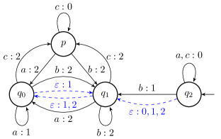
Figure 1: A 2-automaton recognising $W=\mathtt{No}(b)\vee\mathtt{Fin}(aa)\vee{\mathtt{Inf}}(cc)$, where $p$ is assumed to have a different memory state than $q_{0},q_{1}$ and $q_{2}$. It is $2$-wise $\varepsilon$-completable by adding the indicated $\varepsilon$-transitions. A completion also contains the transitions $q_{2}\xrightarrow{\varepsilon:0,1,2}q_{0}$, omitted for ease of reading. However, it is not chromatic since reading $c$ may or may not switch the memory state.

The following theorem, a key result in [10] where it is called the structuration lemma, will also be crucial to this work. Recall that we see well-founded pointed graphs as automata with only $0$-transitions, and we apply the terms $k$-blowup and $\varepsilon$-completable to them accordingly.

Theorem 2.3 (Adapted from Lemma 3.4 in [10]).

Let $G$ be a well-founded pointed graph satisfying an objective $W$ which is assumed to have (chromatic) memory $\leq k$ over games of size $\leq 2^{|G|}$. There is a (chromatic) $k$-blowup $G^{\prime}$ of $G$ which is well-founded, $k$-wise $\varepsilon$-complete, and satisfies $W$.

For completeness, we give a proof of Theorem 2.3 in Appendix A.

Universal graphs.

Given an objective $W$ and a cardinal $\kappa$, we say that a graph $U$ is $(\kappa,W)$-universal if for any infinite tree $T$ of cardinality $|V(T)|<\kappa$ satisfying $W$, there is a morphism $\phi:T\to U$ such that $\phi(t_{0})$ satifies $W$ in $U$, where $t_{0}$ is the root of $T$. We may now rephrase the main theorem of [10] in terms of $\varepsilon$-complete universal graphs.

Theorem 2.4 (Theorem 3.1 in [10]).

Let $W$ be an objective. Then $W$ has (chromatic) memory $\leq k$ if and only if for every cardinal $\kappa$ there exists a $(\kappa,W)$-universal graph which is (chromatic and) $k$-wise $\varepsilon$-complete.

We now give an explicit definition of a $(\kappa,\mathrm{Parity}_{d})$-universal graph $S^{\kappa}_{d}$ which is $\varepsilon$-complete. These ideas date back to the works of Streett and Emerson, who coined the name signatures [26], and were made more explicit by Walukiewicz [28]. Vertices are tuples of ordinals $<\kappa$, indexed by odd priorities in $d$ and ordered lexicographically (with the smaller indices being the most significant). For a tuple $s$ and index $y$, we let $s_{<y}$ be the tuple obtained from $s$ by restricting to coordinates with index $<y$. Edges are given by

$$s\xrightarrow{y}s\quad\iff\quad\begin{cases}s_{<y}\geq s^{\prime}_{<y}\text{ and $y$ is even; or}\\ s_{\leq y}>s^{\prime}_{\leq y}\text{ and $y$ is odd,}\end{cases}$$

and $\varepsilon$-edges are given by $s\xrightarrow{\varepsilon}s^{\prime}$ if and only if $s\geq s^{\prime}$.

Lemma 2.5 ([9, Lemma 2.7]).

The graph $S^{\kappa}_{d}$ is $(\kappa,\mathrm{Parity}_{d})$-universal.

We will work extensively with such tuples, as well as their prefixes and suffixes. For readability, we also use subscripts to indicate which (odd) coordinates are concerned, for instance $s_{<x}$ will be our notation for tuples of ordinals $<\kappa$ indexed with odd priorities $<x$, and similarly for $s_{>x}$. Concatenation of tuples is written like for words, therefore $s_{<x}s_{>x}$ denotes a tuple indexed by all odd priorities (i.e. an vertex of $S_{\kappa}^{d}$). We treat $s_{<x}$ and $s_{>x}$ as different variables, which we may quantify independently.

3 Characterisation of objectives in $\text{BC}(\mathbf{\Sigma}^{0}_{2})$ with memory $\leq k$

We state our main characterisation theorem and its decidability consequences for $\omega$-regular languages. We assume that the alphabet $\Sigma$ is countable, therefore automata can also be taken with countable sets of states.

Theorem 3.1 (Main characterisation).

Let $W$ be a $\mathrm{BC}(\mathbf{\Sigma}^{0}_{2})$ objective and let $k\in\mathbb{N}$. The following are equivalent:

1. $W$ has memory $\leq k$ (resp. chromatic memory $\leq k$) on games of size $\leq 2^{2^{\aleph_{0}}}$.

2. For any automaton $\mathcal{A}$ recognising $W$, there is a (chromatic) $k$-blowup $\mathcal{B}$ of $\mathcal{A}$ which is $k$-wise $\varepsilon$-complete and recognises $W$.

3. There is a deterministic (chromatic) $k$-automaton $\mathcal{A}$ which is $k$-wise $\varepsilon$-completable and recognises $W$. If $W$ is recognised by a deterministic automaton of size $n$, then $\mathcal{A}$ can be taken of size $kn$.

4. For every cardinal $\kappa$, there is a (chromatic) $(\kappa,W)$-universal graph which is well-founded and $k$-wise $\varepsilon$-complete.

5. $W$ has (chromatic) memory $\leq k$ on arbitrary games.

For $\omega$-regular $W$ given by a deterministic automaton $\mathcal{B}$ of size $n$, this allows to compute the (chromatic) memory in NP: guess a deterministic automaton $\mathcal{A}$ of size $\leq kn$ and a (chromatic) $k$-wise $\varepsilon$-completion $\mathcal{A}^{\varepsilon}$, and check if $L(\mathcal{B})\subseteq L(\mathcal{A})$ and if $L(\mathcal{A}^{\varepsilon})\subseteq L(\mathcal{B})$, which can be done in polynomial time, since $\mathcal{A}$ and $\mathcal{B}$ are deterministic [11]. Prior to our work, neither computing the memory nor the chromatic memory was known to be decidable (although the chromatic memory over finite graphs can be computed in exponential time [20]).

Corollary 3.2 (Decidability in NP).

Given an integer $k$ and a deterministic automaton $\mathcal{A}$, the problem of deciding if $L(\mathcal{A})$ has (chromatic) memory $\leq k$ belongs to NP.

Our main contribution is the implication from (i) to (ii), which is the object of Section 3.1. We proceed in Section 3.2 to show that (ii) implies (iii) which is straightforward. The implication (iii) $\implies$ (iv) is adapted from [8] and presented in Section 3.3. Finally, the implication (iv) $\implies$ (v) is the result of [10] (Theorem 2.4), and the remaining one is trivial.

3.1 Existence of $k$-wise $\varepsilon$-complete automata: Proof overview

We start with the more challenging and innovative implication: how to obtain a $k$-wise $\varepsilon$-complete automaton given an objective in $\text{BC}(\mathbf{\Sigma}^{0}_{2})$ with memory $k$ (that is, (i) $\implies$ (ii)). In this Section, we give a detail overview of the proof. Full details are given in Appendix B.

Proposition 3.3.

Let $W$ be an objective recognised by an automaton $\mathcal{A}$, and assume that $W$ has (chromatic) memory $\leq k$ on games of size $\leq 2^{2^{\aleph_{0}}}$. Then there is a (chromatic) $k$-blowup $\mathcal{B}$ of $\mathcal{A}$ recognising $W$ which is $k$-wise $\varepsilon$-complete.

We assume that $W$ has memory $\leq k$ on games of size $\leq\kappa$; we discuss the chromatic case at the end of the section. Let $\mathcal{A}$ be an automaton recognising $W$; we aim to construct a $k$-blowup $\mathcal{B}$ of $\mathcal{A}$ which is $\varepsilon$-complete. We let $S$ denote $S^{\kappa}_{d}$, the $(\kappa,\mathrm{Parity}_{d})$-universal graph defined above.

We consider the cascade product $\mathcal{A}\ltimes S$; this is a $(\Sigma\cup\{\varepsilon\})$-graph which intuitively encodes all possible accepting behaviours in $\mathcal{A}$. Then we apply the structuration result (Theorem 2.3) to $\mathcal{A}\ltimes S$ which yields a $k$-blowup $G$ of $\mathcal{A}\ltimes S$ which is well-founded and $k$-wise $\varepsilon$-complete (as a graph). Stated differently, up to blowing the graph $\mathcal{A}\ltimes S$ into $k$ copies, we have been able to endow it with many $\varepsilon$-transitions, so that over each copy, $\xrightarrow{\varepsilon}$ defines a well-order. Note that the states of $G$ are of the form $(q,m,s)$, with $q\in V(\mathcal{A})$, $m\in\{1,\dots,k\}$ and $s\in V(S)$.

The states of $\mathcal{B}$ will be $V(\mathcal{B})=V(\mathcal{A})\times\{1,\dots,k\}$. The challenge lies in defining the transitions in $\mathcal{B}$, based on those of $G$.

Given a state $(q,m)\in V(\mathcal{B})$ and a transition $q\xrightarrow{c:y}q^{\prime}$ in $\mathcal{A}$, where $c\in\Sigma\cup\{\varepsilon\}$, by applying the definitions we get transitions of the form $(q,m,s)\xrightarrow{c}(q^{\prime},m^{\prime},s^{\prime})$ in $G$, for different values of $m^{\prime}$, whenever $s\xrightarrow{y}s^{\prime}$ in $S$. We will therefore define transition $(q,m)\xrightarrow{c:y}(q^{\prime},m^{\prime})$ in $\mathcal{B}^{\varepsilon}$ if $m^{\prime}$ matches suitably many transitions as above; for now, we postpone the precise definition.

We should then verify that the obtained automaton $\mathcal{B}$:

• is a $k$-blowup of $\mathcal{A}$,

• is $\varepsilon$-complete, and

• recognises $W$.

The first two items above state that $\mathcal{B}$ should have many transitions: at least those inherited from $\mathcal{A}$, and in addition a number of $\varepsilon$-transitions. This creates a tension with the third item, which states that even with all these added transitions, the automaton $\mathcal{B}$ should not accept too many words.

Let us focus on the third item for now, which will lead to a correct definition for $\mathcal{B}$. Take an accepting run

$$(q_{0},m_{0})\xrightarrow{c_{0}:y_{0}}(q_{1},m_{1})\xrightarrow{c_{1},y_{1}}\dots$$

in $\mathcal{B}$, where $x=\liminf_{i}y_{i}$ is even; for the sake of simplicity, assume that all $y_{i}$’s are $\geq x$. We should show that its labelling $w=c_{0}c_{1}\dots$ belongs to $W$. To this end, we will decorate the run with labels $s_{0},s_{1},\dots\in S$ so that

$$(q_{0},m_{0},s_{0})\xrightarrow{c_{0}}(q_{1},m_{1},s_{1})\xrightarrow{c_{1}}\dots$$

defines a path in $G$, which concludes since $G$ satisfies $W$.

Recall that the elements of $S$ are tuples of ordinals $<\kappa$ indexed by $d/2$ odd priorities. We use $s_{<x}$ (resp. $s_{>}x$)to refer to a tuple indexed by priorities up to $x-1$ (resp. from $x+1$).

To construct the $s_{i}$’s, we fix a well chosen prefix $s_{<x}\in\kappa^{x_{\mathrm{odd}}}$ which will be constant, and proceed as follows.

1. If $y_{i}=x$, then we set $s_{i}=s_{<x}s_{>x}$, for some $s_{>x}$ which depends only on $c_{i}$.

2. If $y_{i}<x$, then we set $s_{i}=s_{<x}s_{>x}$, for some $s_{>x}$ which depends on $c_{i}$ as well as $s_{i+1}$.

At this stage the reader may be worried that the backward induction underlying the above definition is not well-founded; however, since the first case occurs infinitely often, the backward induction from the second item is only performed over finite blocks (see also Figure 2 in Appendix B).

This leads to the following definition for $\mathcal{B}$, where $x$ is an even priority:

$$\begin{array}[]{rcl}(q,m)\xrightarrow{c:x}(q^{\prime},m^{\prime})\text{ in }\mathcal{B}&\iff&\exists s_{<x}\exists s_{>x}\forall s^{\prime}_{>x},(q,m,s_{<x}s_{>x})\xrightarrow{c}(q^{\prime},m^{\prime},s_{<x}s^{\prime}_{>x})\text{ in }G,\\ (q,m)\xrightarrow{c:x+1}(q^{\prime},m^{\prime})\text{ in }\mathcal{B}&\iff&\exists s_{<x}\forall s^{\prime}_{>x}\exists s_{>x},(q,m,s_{<x}s_{>x})\xrightarrow{c}(q^{\prime},m^{\prime},s_{<x}s^{\prime}_{>x})\text{ in }G.\end{array}$$

The first line corresponds to point (a.) above, where $s_{>x}$ can be chosen independently of $s^{\prime}_{>x}$, whereas the second line corresponds to point (b.), since the choice of $s_{>x}$ is conditioned on the value of $s^{\prime}_{>x}$. (For priorities $>x+1$, we may apply either the first or second line, depending on the parity, to get the required conclusion.)

The remaining issue is that the choice of the fixed common prefix $s_{<x}$ should be made uniformly, regardless of the transition. This is achieved thanks to an adequate extraction lemma (which extends the pigeonhole principle to the case at hands), which finds a large enough subset $T$ of $\kappa^{[d]_{\mathrm{odd}}}$, so that transitions $(q,m,s)\xrightarrow{}(q^{\prime},m^{\prime},s^{\prime})$ are similar for different choices of $s,s^{\prime}\in T$. This ensures that $s_{<x}$ can be chosen uniformly.

There remains to verify that $\mathcal{B}$ is indeed a $k$-blowup of $\mathcal{A}$ and that it is $\varepsilon$-complete, which will follow easily from the definitions and $\varepsilon$-completeness of $G$ (this is because, after removing “$\exists s_{<x}$” from the definition above, the second line resemble the negation of the first).

For the chromatic case, the proof is exactly the same, we should simply check that if $G$ is chromatic (which is guaranteed by Theorem 2.3), then the so is the obtained automaton $\mathcal{B}$.

3.2 Existence of deterministic $\varepsilon$-completable automata

We now prove the implication from (ii) to (iii) in Theorem 3.1. Take $\mathcal{A}$ to be a deterministic automaton recognising $W$, and let $\mathcal{B}^{\varepsilon}$ be the obtained $k$-blowup of $\mathcal{A}$ which is (chromatically) $k$-wise $\varepsilon$-complete and recognises $W$. Then let $\mathcal{B}$ be obtained from $\mathcal{B}^{\varepsilon}$ by only keeping, for each state $(q,m)\in V(\mathcal{B})$ and each transition $q\xrightarrow{a:y}q^{\prime}$ in $\mathcal{A}$, a single transition of the form $(q,m)\xrightarrow{a:y}(q^{\prime},m^{\prime})$ chosen arbitrarily. Note that $\mathcal{B}$ is a $k$-blowup of $\mathcal{A}$, so we have: $L(\mathcal{A})\subseteq L(\mathcal{B})\subseteq L(\mathcal{B}^{\varepsilon})$. We conclude that $\mathcal{B}$ is a deterministic (chromatically) $k$-wise $\varepsilon$-completable automaton recognising $W$, as required.

3.3 From deterministic $\varepsilon$-completable automata to universal graphs

We now prove the implication from (iii) to (iv) in Theorem 3.1. This result was already proved in [9, Prop. 5.30] for the case of $k=1$; extending to greater values for $k$ presents no difficulty.

Let $\mathcal{B}$ be a deterministic (chromatic) $k$-wise $\varepsilon$-completable automaton recognising $W$ and $\mathcal{B}^{\varepsilon}$ be an $\varepsilon$-completion. Fix a cardinal $\kappa$ and let $S$ denote $S_{d}^{\kappa}$. Consider the cascade product $U=\mathcal{B}^{\varepsilon}\ltimes S$. We claim that $U$ is (chromatic) $k$-wise $\varepsilon$-complete and $(\kappa,W)$-universal. Universality follows from the facts that $\mathcal{B}$ is deterministic and $S$ is $(\kappa,\mathrm{Parity}_{d})$-universal.

Claim 1.

The graph $U=\mathcal{B}^{\varepsilon}\ltimes S$ is $(\kappa,W)$-universal.

Take a tree $T$ of size $<\kappa$ which satisfies $W$. We should show that $T\to U$. Since $\mathcal{B}$ is deterministic, we can define a labelling $\rho\colon V(T)\to V(\mathcal{B})$ by mapping $t_{0}$ to $q_{0}$ and $t\mapsto q$ if the run of $\mathcal{B}$ on the finite word labelling the path $t_{0}\xrightarrow{}t$ ends in $q$. Then, any infinite path from $t_{0}$ in $T$ is mapped to a run in $\mathcal{B}$ that is accepting (since $T$ satisfies $W$). Therefore the tree $T^{\prime}$ obtained by taking $T$ and replacing edge-labels by the priorities appearing in their $\rho$-images satisfies $\mathrm{Parity}_{d}$ and has size $<\kappa$, so there is a morphism $\mu:T\to S$. It is a direct check that $(\rho,\mu)\colon V(T)\to V(\mathcal{B})\times V(S)=V(U)$ indeed defines a morphism.

Showing that $U$ is $k$-wise $\varepsilon$-complete is slightly trickier.

Claim 2.

The graph $U=\mathcal{B}^{\varepsilon}\ltimes S$ is well-founded and (chromatic) $k$-wise $\varepsilon$-complete.

Well-foundedness of $U$ follows directly from Lemma 2.1. Let us write $B_{1},\dots,B_{k}$ for the $k$ parts of $\mathcal{B}^{\varepsilon}$; the $k$ parts of $U$ will be $B_{1}\times V(S),\dots,B_{k}\times V(S)$. If applicable, chromaticity is a direct check. Let $(b,s),(b^{\prime},s^{\prime})\in V(U)$ be in the same part, i.e. $b,b^{\prime}\in B_{i}$ for some $i$. Let $x_{0}$ be the minimal even priority such that $b\xrightarrow{\varepsilon:x_{0}}b^{\prime}$ in $\mathcal{B}^{\varepsilon}$ (if such an $x$ does not exist then $x_{0}=d+2$). Then let $y_{0}$ be the minimal odd priority such that $s^{\prime}_{\leq y_{0}}>s_{\leq y_{0}}$ (as previously, if $s=s^{\prime}$ then we let $y_{0}=d+1$). We distinguish two cases.

1. If $x_{0}<y_{0}$. Then we have $b\xrightarrow{\varepsilon:x_{0}}b^{\prime}$ in $\mathcal{B}^{\varepsilon}$ and $s_{<x_{0}}=s^{\prime}_{<x_{0}}$ which gives $s\xrightarrow{x_{0}}s^{\prime}$ in $S$. Thus we get $(b,s)\xrightarrow{\varepsilon}(b^{\prime},s^{\prime})$ in $U$.

2. If $y_{0}<x_{0}$. Then $s^{\prime}_{\leq y_{0}}>s_{\leq y_{0}}$, which gives $s^{\prime}\xrightarrow{y_{0}}s$ in $S$. Since $\mathcal{B}^{\varepsilon}$ is $k$-wise $\varepsilon$-completable and by definition of $x_{0}$, we also have $b^{\prime}\xrightarrow{\varepsilon:y_{0}}b$ in $\mathcal{B}^{\varepsilon}$, therefore $(b^{\prime},s^{\prime})\xrightarrow{\varepsilon}(b,s)$ in $U$.

We conclude that either $(b,s)\xrightarrow{\varepsilon}(b^{\prime},s^{\prime})$ or $(b^{\prime},s^{\prime})\xrightarrow{\varepsilon}(b,s)$, as required.

4 Union of objectives

In this section, we establish a strong form of the generalised Kopczyński conjecture for $\mathrm{BC}(\mathbf{\Sigma}^{0}_{2})$ objectives. An objective $W\subseteq\Sigma^{\omega}$ is prefix-increasing if for all $a\in\Sigma$ and $w\in\Sigma^{\omega}$, it holds that if $w\in W$ then $aw\in W$. In words, one remains in $W$ when adding a finite prefix to a word of $w$. Examples of prefix-increasing objectives include prefix-independent and closed objectives. inline,size=,backgroundcolor=yellow]Other interesting clases? - Antonio

Theorem 4.1.

Let $W_{1},W_{2}\subseteq\SS^{\omega}$ be two $\text{BC}(\mathbf{\Sigma}^{0}_{2})$ objectives over the same alphabet, such that $W_{2}$ is prefix-increasing. Assume that $W_{1}$ has memory $\leq k_{1}$ and $W_{2}$ has memory $\leq k_{2}$. Then $W_{1}\cup W_{2}$ has memory $\leq k_{1}k_{2}$.

Remark 4.2.

The assumption that one of the two objectives is prefix-increasing is indeed required: for instance if $W_{1}=aa(a+b)^{\omega}$ and $W_{2}=bb(a+b)^{\omega}$, which are positional but not prefix-increasing, the union $(aa+bb)(a+b)^{\omega}$ is not positional (it has memory $2$).

Remark 4.3.

The bound $k_{1}k_{2}$ in Theorem 4.1 is tight: For every $k_{1},k_{2}$, there are objectives $W_{1}$, $W_{2}$ with memories $k_{1},k_{2}$ respectively, such that $W_{1}\cup W_{2}$ has memory exactly $k_{1}k_{2}$. One such example is as follows: let $\SS=\{a_{1},\dots,a_{k_{1}},b_{1},\dots,b_{k_{2}}\}$ and $W_{1}=\{w\mid w\text{ contains at }\text{least }\text{two }\text{different }a_{i}\text{ infinitely often}\}$ and $W_{2}=\{w\mid w$ contains at least two $b_{i}$ infinitely often$\}$. We can see that $W_{1}$, $W_{2}$ and $W_{1}\cup W_{2}$ have memory, respectively, $k_{1},k_{2}$, and $k_{1}\cdot k_{2}$ by building the Zielonka tree of these objectives and applying [15, Thms. 6, 14].

The rest of the section is devoted to the proof of Theorem 4.1. We explicit a construction for the union of two parity automata, inspired from the Zielonka tree of the union of two parity conditions, and show that it is $(k_{1}k_{2})$-wise $\varepsilon$-completable.

Union of parity languages.

We give an explicit construction of a deterministic parity automaton $\mathcal{T}$ recognising the union of two parity languages, which may be of independent interest. This corresponds to the automaton given by the Zielonka tree of the union (a reduced and structured version of the LAR).

We let $[d_{1}]=\{0,1,\dots,d_{1}\}$ and $[d_{2}]^{*}=\{1^{*},\dots,d_{2}^{*}\}$. Let $[d_{1}]_{\mathrm{odd}}$ and $[d_{2}]^{*}_{\mathrm{odd}}$ denote the restrictions of $[d_{1}]$ and $[d_{2}]^{*}$ to odd elements. By a slight abuse of notation, we sometimes treat elements in $[d_{2}]^{*}$ as natural numbers (e.g. when comparing them).

Alphabet. The input alphabet is $[d_{1}]\times[d_{2}]^{*}$, and we write letters as $(y,z)$. The index of $\mathcal{T}$ is $d_{1}+d_{2}$, we use the letter $t$ for its output priorities.

States. States are given by interleavings of two strictly increasing sequences of $[d_{1}]_{\mathrm{odd}}$ and $[d_{2}]^{*}_{\mathrm{odd}}$. Any state can be taken as initial. For instance, for $d_{1}=d_{2}=6$, an example of a state is:

$$\hskip 42.67912pt\tau=\langle\leavevmode\hbox to0pt{\vbox to0pt{\text{[drawing]}}}1,\leavevmode\hbox to0pt{\vbox to0pt{\text{[drawing]}}}3,\leavevmode\hbox to0pt{\vbox to0pt{\text{[drawing]}}}1^{*},\leavevmode\hbox to0pt{\vbox to0pt{\text{[drawing]}}}5,\leavevmode\hbox to0pt{\vbox to0pt{\text{[drawing]}}}3^{*},\leavevmode\hbox to0pt{\vbox to0pt{\text{[drawing]}}}5^{*}\rangle.$$

We use $\tau$ to denote such a sequence, which we index from $1$ to $(d_{1}+d_{2})/2$, and write $\tau[i]$ for its $i$-th element. For $x\in[d_{1}]$, $x$ odd, we let $\mathsf{ind}_{\tau}(x)=i$ for the index such that $\tau[i]=x$. For $x\geq 2$ even, we let $\mathsf{ind}_{\tau}(x)$ be the index $i$ such that $\tau[i]=x-1$. We let $\mathsf{ind}_{\tau}(0)=0$. We use the same notation for $y\in[d_{2}]^{*}$, $y\geq 1$. For example, in the state above, $\mathsf{ind}_{\tau}(2^{*})=3$.

The intuition is that a state stores a local order of importance between input priorities.

Transitions. Let $\tau$ be a state and $(y,z)$ an input letter. We define the transition $\tau\xrightarrow{(y,z):t}\tau^{\prime}$ as follows:

Let $i=\min\{\mathsf{ind}_{\tau}(y),\mathsf{ind}_{\tau}(z)\}$. In the following, we assume $i=\mathsf{ind}_{\tau}(y)$ (the definition for $i=\mathsf{ind}_{\tau}(z)$ is symmetric). We let $t=2i$, if $y$ even, and $t=2i-1$ if $y$ is odd. If $y$ is even, we let $\tau^{\prime}=\tau$. If $y$ is odd, let $i^{\prime}$ be the smallest index $i<i^{\prime}$ such that $\tau[i^{\prime}]\in[d_{2}]^{*}$, and let $\tau^{\prime}$ be the sequence obtained by inserting $\tau[i^{\prime}]$ on the left of $\tau[i]$ (or $\tau^{\prime}=\tau$ if no such index $i^{\prime}$ exists). Formally,

$$\tau^{\prime}[j]=\tau[j]\text{ for }j<i\text{ and }i^{\prime}<j,\quad\tau^{\prime}[i]=\tau[i^{\prime}]\quad\text{ and }\quad\tau^{\prime}[j]=\tau[j-1]\text{ for }i<j\leq i^{\prime}.$$

For example, for the state above, we have: $\langle 1,3,1^{*},5,3^{*},5^{*}\rangle\xrightarrow{(3,2^{*}):3}\langle 1,1^{*},3,5,3^{*},5^{*}\rangle.$

Lemma 4.4.

The automaton $\mathcal{T}$ recognises the language

$$L=\{w\in([d_{1}]\times[d_{2}]^{*})^{\omega}\mid\pi_{1}(w)\in\mathrm{Parity}_{d_{1}}\ \mathrm{or}\ \pi_{2}(w)\in\mathrm{Parity}_{d_{2}}\}.$$

Proof 4.5.

We show that $L\subseteq L(\mathcal{T})$, the other inclusion is similar (and implied by Lemma 4.9 below). Let $(y_{1},z_{1})(y_{2},z_{2})\dots\in W$, and assume w.l.o.g. that $y_{1}y_{2}\dots\in\mathrm{Parity}_{d_{1}}$. Let $y_{\mathrm{min}}=\liminf y_{i}$, which is even, and let $n_{0}$ be so that for all $n\geq n_{0}$ we have $y_{\mathrm{min}}\leq y_{n}$. Let

$$\tau_{0}\xrightarrow{(y_{1},z_{1}):t_{1}}\tau_{1}\xrightarrow{(y_{2},z_{2}):t_{2}}\dots$$

denote the corresponding run in $\mathcal{T}$. Let $i_{n}=\mathsf{ind}_{\tau_{n}}(y_{\mathrm{min}})$ be the index where $y_{\mathrm{min}}-1$ appears in $\tau_{n}$. Note that the sequence $(i_{n})_{n\geq n_{0}}$ is decreasing. Let $n_{1}$ be the moment where this sequence stabilises, i.e., $i_{n}=i_{n_{1}}$ for $n\geq n_{1}$. By definition of the transitions of $\mathcal{T}$, for $n\geq n_{1}$ all output priorities are $\geq 2i_{n_{1}}$, and priority $2i_{n_{1}}$ is produced every time that a letter $(y_{\mathrm{min}},z_{n})$ is read. We conclude that $\mathcal{T}$ accepts $w$.

$0$-freeness of automata for prefix-increasing objectives.

The fact that $W_{2}$ is prefix-increasing will be used via the following lemma. It recasts the fact that we can add $\xrightarrow{\varepsilon:1}$ transitions everywhere to automata recognising prefix-increasing objectives.

Lemma 4.6.

Let $W$ a be prefix-increasing objective with memory $\leq k$. There exists a deterministic $k$-wise $\varepsilon$-completable automaton $\mathcal{A}$ recognising $W$ and an $\varepsilon$-completion $\mathcal{A}^{\varepsilon}$ of $\mathcal{A}$ such that $\mathcal{A}^{\varepsilon}$ does not have any transition with priority $0$.

Proof 4.7.

First, take any automaton $\mathcal{A}_{0}$ recognising $W$. Then let $\mathcal{A}_{1}$ be obtained by shifting every priority from $\mathcal{A}_{0}$ by $2$. Clearly $\mathcal{A}_{1}$ also recognises $W$ and does not have any transition with priority $0$. Then apply Proposition 3.3 to get a $k$-blowup $\mathcal{A}$ of $\mathcal{A}_{1}$ which is $k$-wise $\varepsilon$-completable, and let $\mathcal{A}^{\varepsilon}$ denote the corresponding $\varepsilon$-completion. Since $\mathcal{A}$ has no transition with priority $0$, the only possible such transitions in $\mathcal{A}^{\varepsilon}$ are $\varepsilon$-transition. Then remove all $\varepsilon$-transitions with priority $0$ in $\mathcal{A}^{\varepsilon}$, and add $\xrightarrow{\varepsilon:1}$ transitions between all pairs of states in $\mathcal{A}^{\varepsilon}$ (in both directions).

Clearly, the obtained automaton $\tilde{\mathcal{A}}^{\varepsilon}$ is $\varepsilon$-complete and has no transition with priority $0$. There remains to prove that it recognises $W$. Take an accepting run in $\tilde{\mathcal{A}}^{\varepsilon}$ and observe that the priority $1$ is only seen finitely often. Hence from some moment on, the run coincides with a run in $\mathcal{A}^{\varepsilon}$. We conclude since $W$ is prefix-increasing.

Main proof: $\varepsilon$-completion of the product.

We now proceed with the proof of Theorem 4.1. Using Theorem 3.1, for $l=1,2$, we take deterministic $k_{l}$-wise $\varepsilon$-completable automata $\mathcal{A}_{l}$ of index $d_{l}$ recognising $W_{l}$, and its $\varepsilon$-completion $\mathcal{A}_{l}^{\varepsilon}$. For $l=2$, we assume thanks to Lemma 4.6 that $\mathcal{A}_{2}^{\varepsilon}$ does not have any transition with priority $0$.

We consider the product $\mathcal{A}=(\mathcal{A}_{1}\times\mathcal{A}_{2})\ltimes\mathcal{T}$, with states $V(\mathcal{A}_{1})\times V(\mathcal{A}_{2})\times V(\mathcal{T})$ and transitions $(q_{1},q_{2},\tau)\xrightarrow{a:t}(q^{\prime}_{1},q^{\prime}_{2},\tau^{\prime})$ if $q_{1}\xrightarrow{a:y}q_{1}^{\prime}$ in $\mathcal{A}_{1}$, $q_{2}\xrightarrow{a:z}q_{2}^{\prime}$ in $\mathcal{A}_{2}$, and $\tau\xrightarrow{(y,z):t}\tau^{\prime}$ in $\mathcal{T}$. The correctness of such a construction is folklore.

Claim 3.

The automaton $\mathcal{A}$ is deterministic and recognises $W=W_{1}\cup W_{2}$.

Therefore, there only remains to show the following lemma.

Lemma 4.8.

The automaton $\mathcal{A}=(\mathcal{A}_{1}\times\mathcal{A}_{2})\ltimes\mathcal{T}$ is $(k_{1}k_{2})$-wise $\varepsilon$-completable.

The $\varepsilon$-completion of $\mathcal{A}$ will be a variant of a product of the form $\mathcal{A}_{1}^{\varepsilon}\times\mathcal{A}_{2}^{\varepsilon}\ltimes\overline{\mathcal{T}}$, where $\overline{\mathcal{T}}$ is a non-deterministic extension of $\mathcal{T}$ with more transitions, but which still recognises the same language.

The automaton $\overline{\mathcal{T}}$. Intuitively, we obtain $\overline{\mathcal{T}}$ by allowing to reconfigure the elements of index $>i$ in a state $\tau$ by paying an odd priority $2i-1$, as well as allowing to move elements of $[d_{1}]$ to the left. We precise this idea next.

We order the states of $\mathcal{T}$ lexicographically, where we assume that $x<y$ for $x\in[d_{1}]$ and $y\in[d_{2}]^{*}$. Formally, we let $\tau<\tau^{\prime}$ if for the first position $j$ where $\tau$ and $\tau^{\prime}$ differ, $\tau[j]\in[d_{1}]$ (and therefore necessarily $\tau^{\prime}[j]\in[d_{2}]^{*}$). We let $\tau[..i]$ be the prefix of $\tau$ up to (and including) $\tau[i]$. We write $\tau<_{i}\tau^{\prime}$ if $\tau[..i]<\tau^{\prime}[..i]$.

Let $\tau\xrightarrow{(y,z):t}$ be a transition in $\mathcal{T}$ as above, and $i_{0}=\min\{\mathsf{ind}_{\tau}(y),\mathsf{ind}_{\tau}(z)\}$ be the index determining $t$ (i.e. $t\in\{2i_{0}-1,2i\}$). The automaton $\overline{\mathcal{T}}$ contains a transition $\tau\xrightarrow{(y,z):t^{\prime}}\tau^{\prime}$ if:

1. $t^{\prime}=t$ is odd, and $\tau^{\prime}\leq_{i_{0}-1}\tau$; or

2. $t^{\prime}=t$ is even, and $\tau^{\prime}\leq_{i_{0}}\tau$; or

3. $t^{\prime}\in\{2i^{\prime}-1,2i^{\prime}\}$ for some $i^{\prime}\leq i_{0}$ and $\tau^{\prime}<_{i^{\prime}}\tau$. (Note that, if $t$ is odd, this includes all (possibly even) $t^{\prime}\leq t+1$.)

In words, we are allowed to output a small (i.e. important) priority when following a strict decrease on sufficiently small components in $\tau$. Note that transitions in $\mathcal{T}$ also belong to $\overline{\mathcal{T}}$ thanks to the rules (1) and (2).

Lemma 4.9.

The automaton $\overline{\mathcal{T}}$ recognises the same language as $\mathcal{T}$.

Proof 4.10.

It is clear that $L(\mathcal{T})\subseteq L(\overline{\mathcal{T}})$. We show the other inclusion.

Consider

$$\tau_{0}\xrightarrow{(y_{1},z_{1}):t_{1}}\tau_{1}\xrightarrow{(y_{2},z_{2}):t_{2}}\dots,\quad\text{ an accepting run in }\overline{\mathcal{T}}.$$

Let $t_{\mathrm{min}}=\liminf t_{1}t_{2}\dots$, which is even. Let $i_{\mathrm{min}}=t_{\mathrm{min}}/2$ be the index responsible for producing priority $t_{\mathrm{min}}$. Let $n_{0}$ be such that $t_{n}\geq t_{\mathrm{min}}$ for all $n\geq n_{0}$. Observe that for all $n\geq n_{0}$, we have $\tau_{n}\geq_{(i_{\mathrm{min}}-1)}\tau_{n+1}$, and therefore there is $n_{1}\geq n_{0}$ such that the prefix $\tau_{n}[..i_{\mathrm{min}}-1]$ is the same for all $n\geq n_{1}$. In fact, the prefix $\tau_{n}[..i_{\mathrm{min}}]$ must be constant too, as we can only modify $\tau_{n}[i_{\mathrm{min}}]$ using rule (1.) and that would output priority $t_{\mathrm{min}}-1$. Assume w.l.o.g. that $\tau_{n}[i_{\mathrm{min}}]=y\in[d_{1}]_{\mathrm{odd}}$. Now, for each $n\geq n_{1}$ it must be that $y_{i}\geq y+1$ and it must be that $y_{i}=y+1$ each time that priority $t_{\mathrm{min}}$ is produced. Therefore, $\liminf y_{1}y_{2}\dots=y+1$ is even.

The $\varepsilon$-completion. We define $\mathcal{A}^{\varepsilon}$ as a version of the cascade product of $\mathcal{A}_{1}^{\varepsilon}\times\mathcal{A}_{2}^{\varepsilon}$ with $\mathcal{T}$, in which $\varepsilon$-transitions are also allowed to use the transitions of $\overline{\mathcal{T}}$. We let $\preccurlyeq$ denote the preference ordering over priorities, given by $1\preccurlyeq 3\preccurlyeq\dots\preccurlyeq d-1\preccurlyeq d\preccurlyeq\dots 2\preccurlyeq 0\text{ ($d$ even)}$. The transitions in $\mathcal{A}^{\varepsilon}$ are defined as follows:

• For $a\in\SS$: $(q_{1},q_{2},\tau)\xrightarrow{a:t}(q^{\prime}_{1},q^{\prime}_{2},\tau^{\prime})$ if this transition appears in $(\mathcal{A}_{1}\times\mathcal{A}_{2})\ltimes\mathcal{T}$.

• $(q_{1},q_{2},\tau)\xrightarrow{\varepsilon:t}(q^{\prime}_{1},q^{\prime}_{2},\tau^{\prime})$ if $q_{1}\xrightarrow{\varepsilon:y}q_{1}^{\prime}$ in $\mathcal{A}_{1}^{\varepsilon}$, $q_{2}\xrightarrow{\varepsilon:z}q_{2}^{\prime}$ in $\mathcal{A}_{2}^{\varepsilon}$, and $\tau\xrightarrow{(y,z):t^{\prime}}\tau^{\prime}$ in $\overline{\mathcal{T}}$ with $t^{\prime}\preccurlyeq t$.

Note that the condition $t^{\prime}\preccurlyeq t$ simply allows to output a less favorable priority, so it does not create extra accepting runs. By definition, $\mathcal{A}^{\varepsilon}$ has been obtained by adding $\varepsilon$-transitions to $\mathcal{A}$. It is a folklore result that composition of non-deterministic automata also preserves the language recognised, so this construction is correct.

Claim 4.

The automaton $\mathcal{A}^{\varepsilon}$ recognises $W$.

Therefore, we there only remains to prove the following lemma.

Lemma 4.11.

The automaton $\mathcal{A}^{\varepsilon}$ is $(k_{1}k_{2})$-wise $\varepsilon$-complete.

The formal proof of this statement is presented in Appendix C. The $k_{1}$ parts of $\mathcal{A}_{1}^{\varepsilon}$ and the $k_{2}$ parts of $\mathcal{A}_{2}^{\varepsilon}$ naturally induce a partition of the states of $\mathcal{A}^{\varepsilon}$ into $k_{1}k_{2}$ parts. Then, given two states $r=(q_{1},q_{2},\tau)$ and $r^{\prime}=(q_{1}^{\prime},q_{2}^{\prime},\tau^{\prime})$ in the same part of $\mathcal{A}^{\varepsilon}$, we consider the longest common prefix of $\tau$ and $\tau^{\prime}$. We perform a case analysis: Depending on the priorities of $[d_{1}]$ or $[d_{2}]^{*}$ appearing in this prefix, and the transitions $q_{l}\xrightarrow{\varepsilon:x}q_{l}^{\prime}$ of the automata $\mathcal{A}_{1}^{\varepsilon}$, $\mathcal{A}_{2}^{\varepsilon}$, we will find transitions $r\xrightarrow{\varepsilon:x}r^{\prime}$ or $r^{\prime}\xrightarrow{\varepsilon:x+1}r$ for all even $x$.

5 Conclusions and open questions

We characterised objectives in $\mathrm{BC}(\mathbf{\Sigma}^{0}_{2})$ with memory (or chromatic memory) $\leq k$ as those recognised by a well-identified class of automata. In particular, this gives the first known characterisation of (chromatic) memory for $\omega$-regular objectives, and proves that it is decidable (in fact even in NP). We also settled (a strengthening of) Kopczyński’s conjecture for $\mathrm{BC}(\mathbf{\Sigma}^{0}_{2})$ objectives. We now discuss some directions for future work.

Memory in finite games.

This paper focuses on games over potentially infinite game graphs. A wide body of literature studies the memory over finite game graphs [20, 5]; we believe that, for $\omega$-regular objectives, both notions should coincide, and our results should characterise the memory of $\omega$-regular objectives over finite games too. More precisely, we believe that in item (i) in Theorem 3.1, it suffices to assume that $W$ has memory $\leq k$ over games of size $f(n)$, for some finite bound $f(n)$, where $n$ is the size of a deterministic automaton representing $W$.

Question 5.1 (Version of [27, Conjecture 9.1.2]).

Show that if an $\omega$-regular objective has memory $\leq k$ over finite game graphs, then it has memory $\leq k$ over all game graphs.

The hypothesis on $\omega$-regularity is necessary, as this statement already fails in the case of positionality and closed objectives [13]. We believe that one should be able to adapt the proof of Proposition 3.3 to obtain this result, but some new ideas seem to be required. As a follow-up question one could investigate the bound $f(n)$: can it be assumed polynomial?

Exact complexity of computation of memory.

We established that computing the (chromatic) memory of an $\omega$-regular objective is in NP. In fact, computing the chromatic memory is NP-hard already for simple classes of objectives, such as Muller [7] or safety ones [3]. However, no such hardness results are known for non-chromatic memory.

Question 5.2.

Given a deterministic parity automaton $\mathcal{A}$ and a number $k$, can we decide whether the memory of $L(\mathcal{A})$ is $\leq k$ in polynomial time?

This question is open already for the simpler case of regular open objectives (that is, those recognised by reachability automata).

Assymetric 1-to-2-player lifts.

A celebrated result of Gimbert and Zielonka [18] states that if for an objective $W$ both players can play optimally using positional strategies in finite games where all vertices belong to one player, then $W$ is bipositonal over finite games. This result has been extended in two orthogonal directions: to objectives where both players require finite chromatic memory [5, 4] (symmetric lift for memory), and to $\omega$-regular objectives where Eve can play positionally in $1$-player games [8] (asymmetric lift for positionality). In this work, we have not provided an asymmetric lift for memory, as in most cases no such result can hold. For $\mathrm{BC}(\mathbf{\Sigma}^{0}_{2})$ objectives, it is known to fail already for positional objectives [17, Section 7]. For non-chromatic memory, it cannot hold for $\omega$-regular objectives neither, because of the example described below.

Proposition 5.3.

Let $\Sigma_{n}=\{1,\dots,n\}$. For every $n$, the objective

$$W_{n}=\{w\in\SS_{n}^{\omega}\mid w\text{ contains two different letters infinitely often}\}$$

has memory $2$ over games where Eve controls all vertices and memory $n$ over arbitrary games.

Proof 5.4.

The fact that $W_{n}$ has memory $n$ follows from [15]. We include the proof that it has memory $2$ over games controlled by Eve in Appendix D.

In his PhD thesis, Vandenhove conjectures that an assymetric lift for chromatic memory holds for $\omega$-regular objectives [27, Conjecture 9.1.2]. This question remains open.

Question 5.5.

Is there an $\omega$-regular objective with chromatic memory $k$ over games where Eve controls all vertices and chromatic memory $k^{\prime}>k$ over arbitrary games?

Further decidability results for memory.

As mentioned in the introduction, many extensions of $\omega$-automata (including deterministic $\omega$-Turing machines and unambiguous $\omega$-petri nets [16]) compute languages that are in $\mathrm{BC}(\mathbf{\Sigma}^{0}_{2})$. We believe that our characterisation may lead to decidability results regarding the memory of objectives represented by these models.

Objectives in $\Delta_{0}^{3}$.

Some of the questions answered in this work in the case of $\mathrm{BC}(\mathbf{\Sigma}^{0}_{2})$ objectives are open in full generality, for instance, the generalised Kopczyński’s conjecture. A reasonable next step would be to consider the class $\mathbf{\Delta}^{0}_{3}=\mathbf{\Sigma}^{0}_{3}\cap\mathbf{\Pi}^{0}_{3}$. Objectives in $\mathbf{\Delta}^{0}_{3}$ are those recognised by max-parity automata using infinitely many priorities [25]. Our methods seem appropriate to tackle this class, however, we have been unable to extend the extraction lemma (Lemma B.1) used in the proof of Section 3.1.

Appendix A Proof of Theorem 2.3 (Structuration result)

We now give a proof of Theorem 2.3.

See 2.3

The idea is to use choice arenas, which were introduced in Ohlmann’s PhD thesis [22, Section 3.2 in Chapter 3] for positionality, and then adapted to memory in [8].

Proof A.1.

Let $H$ be the game defined as follows. The set of vertices is $V(G)\sqcup\mathcal{P}_{\neq\varnothing}(V(G))$, where $\mathcal{P}_{\neq\varnothing}(V(G))$ is the set of non-empty subsets $X$ of $V(G)$, partitioned into $V_{\text{Adam}}=V(G)$ and $V_{\text{Eve}}=\mathcal{P}_{\neq\varnothing}(V(G))$. The initial vertex is $v_{0}$, the one of $G$. Then the edges are given by taking those of $G$, and then adding $v\xleftrightarrow{\varepsilon}X$ whenever $v\in X$. The objective is $W$.

In words, when playing in $H$, Adam follows a path of his choice in $G$, except that at any point, he may choose a set $X$ containing the current vertex $v$, and allow Eve to continue the game from any vertex of her choice in $X$. In some sense, Adam can hide the current vertex; this is especially true if Eve is required to play with finite memory.

Since $G$ satisfies $W$, Eve wins, simply by going back to the previous vertex $v$ every time Adam picks an edge $v\xrightarrow{\varepsilon}X$. (Formally, the corresponding winning strategy has vertices $V(G)\sqcup\{(v,X)\mid v\in X\}$, projection $\pi(v)=v$ and $\pi(v,X)=X$, edges $E(G)\cup\{v\xleftrightarrow{\varepsilon}(v,X)\mid v\in X\}$, and initial vertex $v_{0}$.) Therefore by our assumption on $W$, there is a (chromatic) winning strategy $S$ with memory $k$, i.e. $V(S)=V(H)\times\{1,\dots,k\}$.

Now we define $G^{\prime}$ by $V(G^{\prime})=V(G)\times\{1,\dots,k\}$, initial vertex $(v_{0},m_{0})$, the initial vertex of $S$, and with the edges from $E(S)\cap(V(G^{\prime})\times(\Sigma\cup\{\varepsilon\})\times V(G^{\prime}))$, together with edges $(v,m)\xrightarrow{\varepsilon}(v^{\prime},m)$ whenever there is $X\ni v,v^{\prime}$ such that $(X,m)\xrightarrow{\varepsilon}(v^{\prime},m)\text{ in }S$.

We prove that $G^{\prime}$ satisfies the conclusion of the theorem, except for well-foundedness which is dealt with below.

$G^{\prime}$ is a $k$-blowup of $G$.

This is because $S$ is a strategy, and vertices in $V(G)$ belong to Adam in $H$. Therefore, for each $(v,m)\in V(G^{\prime})$, and each edge $v\xrightarrow{c}v^{\prime}$ in $G$, $v\xrightarrow{c}v^{\prime}$ is also an edge in $H$, thus there is $m^{\prime}$ such that $(v,m)\xrightarrow{c}(v^{\prime},m^{\prime})$ is an edge in $G^{\prime}$.

In the chromatic case, $G^{\prime}$ is chromatic.

This is because $S$ is chromatic, therefore by definition of $G^{\prime}$, it is chromatic with the same chromatic update function.

$G^{\prime}$ is $k$-wise $\varepsilon$-complete.

Since it is a graph, we should prove that for each $v,v^{\prime}$ and each $m$, either $(v,m)\xrightarrow{\varepsilon}(v^{\prime},m)$ or $(v^{\prime},m)\xrightarrow{\varepsilon}(v,m)$ in $G$. This follows from applying the definition of $G^{\prime}$ to $X=\{v,v^{\prime}\}$, since either $(X,m)\xrightarrow{\varepsilon}v$ or $(X,m)\xrightarrow{\varepsilon}v^{\prime}$ is an edge in $S$ (because $S$ is without dead-ends).

$G^{\prime}$ satisfies $W$.

This is because $S$ is a winning strategy, and every path in $G^{\prime}$ corresponds to a path in $S$, by replacing each edge $(v,m)\xrightarrow{\varepsilon}(v^{\prime},m)$ by $(v,m)\xrightarrow{\varepsilon}X\xrightarrow{\varepsilon}(v^{\prime},m)$.

There remains a slight technical difficulty, which is that $G^{\prime}$ may have $\xrightarrow{\varepsilon}$-cycles (in fact, it even has all $\varepsilon$-self-loops, by applying the definition to $X$ being a singleton). However for each memory state $m$, the relation $\xrightarrow{\varepsilon}$ has the property that for every subset of states $X$, there is $v\in X$ (which should be seen as a minimal element) such that every $v^{\prime}\in X$ satisfies $(v^{\prime},m)\xrightarrow{\varepsilon}(v,m)$ in $G^{\prime}$.

Therefore for each $m$, and each $X\subseteq V(G)$ such that $X\times\{m\}$ is a strongly connected component for $\xrightarrow{\varepsilon}$ in $G^{\prime}$, we pick an arbitrary strict well-order $\xrightarrow{}$ over $X$ which extends the $\varepsilon$-edges already present in $G$ over $X$. This is possible because $G$ is assumed $G$ to be well-founded (and it is necessary so that the obtained graph remains a $k$-blowup of $G$). Finally, we rewire $\varepsilon$-edges over $X\times\{m\}$ so that they correspond to $\xrightarrow{}$; it is not hard to see that the above points are not broken by this construction.

Appendix B Full proof of (i) $\implies$ (ii) in Theorem 3.1 (Existence of $k$-wise $\varepsilon$-complete automata)

We prove the following proposition.

See 3.3

We let $\kappa=2^{\aleph_{0}}$ and let $S$ denote $S_{d}^{\kappa}$. Our goal is to define a (chromatic) $k$-blowup $\mathcal{B}$ of $\mathcal{A}$ which is $k$-wise $\varepsilon$-complete and recognises $W$. For now, we discuss general memory, and explain below how the proof is (very easily) adapted to the chromatic case.

We start with the extraction lemma mentioned in the overview, then we will present the definition of $\mathcal{B}$ and then prove its correctness.

B.1 A combinatorial lemma: Extracting homogeneous subtrees

As an important part of our proof, we will take the graph $S$, whose set of vertices is $\kappa^{[d]_{\mathrm{odd}}}$, where $[d]_{\mathrm{odd}}=\{1,3,\dots,d-1\}$, and extract from it a large enough subgraph which is homogeneous. This requires a combinatorial lemma which we now describe.

By a slight abuse of terminology (since this is not consistent with the definition of trees from the preliminaries), we use the terminology “signature trees” to refer to subsets of $\kappa^{[d]_{\mathrm{odd}}}$. Elements of the subsets should be thought of as leaves of the tree, while their (non-proper) prefixes correspond to nodes. More precisely, a node of level $x$, where $x$ is an even priority from $[d]$, in a signature tree $T$ is a tuple $s_{<x}\in\kappa^{x_{\mathrm{odd}}}$ such that there exists $s_{>x}$ satisfying $s_{<x}s_{>x}\in T$.

The subtree rooted at a node $s_{<x}$ of level $x$ is defined to be the tree $\{s_{>x}\mid s_{<x}s_{>x}\in T\}$. We say that a tree $T$ is everywhere cofinal if for each node $s_{<x}$, the subtree rooted at $x$ is cofinal in $\kappa^{(d-x)_{\mathrm{odd}}}$. An inner labelling of a tree $T$ by $L$ is a map $\lambda$ assigning a label in $L$ to every node in $T$. We are now ready to state the extraction lemma We let $\kappa=2^{\aleph_{0}}$.

Lemma B.1.

Let $\lambda$ be an inner labelling of $\kappa^{d_{\mathrm{odd}}}$ by $L$, where $L$ is countable. There is an everywhere cofinal tree $T$ such that at every level $x$, $\lambda$ is constant over nodes of level $x$.

We say that a labelling as in the conclusion of the lemma is constant per level.

Proof B.2.

We prove the lemma by induction on $d$. For $d=0$ there is nothing to prove since $d_{\mathrm{odd}}$ is empty; let $d\geq 1$ and assume the result known for $d-2$. For each node $s$ at level $2$, apply the induction hypothesis on the subtree of $\kappa^{d_{\mathrm{odd}}}$ rooted at $s_{<2}$, which gives an everywhere cofinal tree $T^{\prime}$ and a labelling $\lambda^{\prime}$ which is constant per level over $T^{\prime}$. Let $\ell^{\prime}_{0},\ell^{\prime}_{2},\dots,\ell^{\prime}_{d-2}$ denote the constant values of $\lambda^{\prime}$ on the corresponding levels of $T^{\prime}$, and define the new labelling of $s$ to be the tuple $(\lambda(s),\ell^{\prime}_{0},\dots,\ell^{\prime}_{d-2})$.

Now since there are at most countably-many new labellings, and there are $\kappa=2^{\aleph_{0}}$ nodes at level $2$, there is a new labelling $\ell$ such that cofinaly-many nodes have this new labelling. We conclude by taking $T$ to be the union of $\{s\}\times T^{\prime}_{s}$, where $s$ ranges over nodes at level $2$ with the new labelling $\ell$, and $T^{\prime}_{s}$ are the corresponding everywhere cofinal trees.

B.2 Definition of $\mathcal{B}$

Consider the cascade product $\mathcal{A}\ltimes S$. By Lemma 2.1, it satisfies $W$ and is well-founded. Moreover it has size $\leq\kappa$, so by our assumption on $W$, we may apply Theorem 2.3. This yields a $k$-blowup $G$ of ${\mathcal{A}\ltimes S}$ which is $k$-wise $\varepsilon$-complete. Let us write $V(G)=V(\mathcal{A})\times\{1,\dots,k\}\times V(S)$. We close $G$ by transitivity, meaning that we add transitions $(q,m,s)\xrightarrow{c}(q^{\prime},m^{\prime},s^{\prime})$, for $c\in\Sigma\ {\cup}\left\{\varepsilon\right\}$, whenever $(q,m,s)\xrightarrow{\varepsilon^{*}c\varepsilon^{*}}(q^{\prime},m,s^{\prime})$; the obtained graph $\overline{G}$ still satisfies $W$.

Here comes the important definition: say that $(q,m)$ strongly $c$-dominates $(q^{\prime},m^{\prime})$ at node $s_{<x}$ if

$$\exists s_{>x}\forall s^{\prime}_{>x}\qquad(q,m,s_{<x}s_{>x})\xrightarrow{c}(q^{\prime},m^{\prime},s_{<x}s^{\prime}_{>x})\text{ in }\overline{G},$$

and that $(q,m)$ weakly $c$-dominates $(q^{\prime},m^{\prime})$ at $s_{<x}$ if

$$\forall s^{\prime}_{>x}\exists s_{>x}\qquad(q,m,s_{<x}s_{>x})\xrightarrow{c}(q^{\prime},m^{\prime},s_{<x}s^{\prime}_{>x})\text{ in }\overline{G},$$

where $c\in\Sigma\ {\cup}\left\{\varepsilon\right\}$. Note that strong domination implies weak domination. The type of a node $s_{<x}$ is the information, for each $q,q^{\prime},m,m^{\prime}$ and $c$, of whether $(q,m)$ strongly or weakly (or not at all) $c$-dominates $(q^{\prime},m^{\prime})$. This gives finitely-many possibilities for fixed $q,q^{\prime},m,m^{\prime}$ and $c$, and therefore there are in total a countable number of possible types. Thus Lemma B.1 yields a tree $T\subseteq\kappa^{\alpha}$ which is everywhere cofinal and such that for all $x$, nodes at level $x$ in $T$ all have the same type $t_{x}$.

We are now ready to define $\mathcal{B}$. We put $V(\mathcal{B})=V(\mathcal{A})\times\{1,\dots,k\}$, and for each even $x\in[d]$ and $c\in\Sigma\ {\cup}\left\{\varepsilon\right\}$, we define transitions by

$$\begin{array}[]{lcrl}(q,m)&\xrightarrow{c:x}&(q^{\prime},m^{\prime})&\text{ if }(q,m)\text{ strongly $c$-dominates }(q^{\prime},m^{\prime})\text{ in }t_{x}\\ (q,m)&\xrightarrow{c:x+1}&(q^{\prime},m^{\prime})&\text{ if }(q,m)\text{ weakly $c$-dominates }(q^{\prime},m^{\prime})\text{ in }t_{x}.\end{array}$$

Here is the main lemma, which proves the direct implication in Theorem 3.1.

Lemma B.3.

Automaton $\mathcal{B}$ is a $k$-blowup of $\mathcal{A}$, it is $k$-wise $\varepsilon$-complete and it recognises $W$.

The remainder of the section is devoted to proving Lemma B.3.

B.3 Correctness of $\mathcal{B}$: Proof of Lemma B.3

There are a few things to show. The interesting argument is the one that shows that $\mathcal{B}$ recognises $W$ (Lemma B.8 below). We should also prove there is no accepting run over words in $\Sigma^{*}\varepsilon^{\omega}$, which will be done below as part of Lemma B.8.

$\mathcal{B}$ is a $k$-blowup of $\mathcal{A}$.

We should prove the following.

Claim 5.

For all transitions $q\xrightarrow{a:y}q^{\prime}$ in $\mathcal{A}$, and any $m\in\{1,\dots,k\}$ there is some $m^{\prime}\in\{1,\dots,k\}$ such that $(q,m)\xrightarrow{a:y}(q^{\prime},m^{\prime})$ in $\mathcal{B}$.

Let $q\xrightarrow{a:y}q^{\prime}$ be a transition in $\mathcal{A}$ and let $m\in\{1,\dots,k\}$. Since $G$ is a $k$-blowup of $\mathcal{A}\times S$, for all edges $s\xrightarrow{y}s^{\prime}$ in $S$ there is $m^{\prime}\in\{1,\dots,k\}$ such that $(q,m,s)\xrightarrow{a}(q^{\prime},m^{\prime},s^{\prime})\text{ in }G$. Although both proofs are similar, we distinguish two cases.

• If $y=x$ is even. We prove that for all nodes $s_{<x}$ at level $x$, $(q,m)$ strongly $c$-dominates $(q^{\prime},m^{\prime})$ for some $m^{\prime}$. Therefore the same is true in $t_{x}$ which implies the wanted result. We let $s_{>x}=0_{>x}$, the zero sequence in $\kappa^{(d-x)_{\mathrm{odd}}}$. Now for all $s^{\prime}_{>x}\in\kappa^{(d-x)_{\mathrm{odd}}}$, it holds that $s_{<x}s_{>x}=s_{<x}0_{>x}\xrightarrow{x}s_{<x}s^{\prime}_{>x}$ in $S$, so there is $m^{\prime}$ such that $(q,m,s_{<x}s_{>x})\xrightarrow{a}(q,m^{\prime},s_{<x}s^{\prime}_{>x})$ in $G$ and thus also in $\overline{G}$; in this case say that $m^{\prime}$ is good for $s^{\prime}_{>x}$.

  Now we claim that if $m^{\prime}$ is good for $\tilde{s}^{\prime}_{>x}\geq s^{\prime}_{>x}$, then it is also good for $s^{\prime}_{>x}$. Indeed, we have $(q^{\prime},s_{<x}\tilde{s}^{\prime}_{>x})\xrightarrow{\varepsilon}(q^{\prime},s_{<x}s^{\prime}_{>x})$ in $\mathcal{A}\times S$ therefore since $\varepsilon$-transitions preserve the memory state in $G$ (Theorem 2.3) we have $(q^{\prime},m^{\prime},s_{<x}\tilde{s}^{\prime}_{>x})\xrightarrow{\varepsilon}(q^{\prime},m^{\prime},s_{<x}s^{\prime}_{>x})$ in $G$ thus $(q,m,s_{<x}s_{>x})\xrightarrow{a}(q^{\prime},m^{\prime},s_{<x}s^{\prime}_{>x})$ in $\overline{G}$.

  Therefore the sets $M^{\prime}_{s^{\prime}_{>x}}$ of $m^{\prime}$ which are good for $s^{\prime}_{>x}$ form a decreasing chain of non-empty subsets of $\{1,\dots,k\}$ and thus their intersection is non-empty: there is some $m^{\prime}$ which is good for all $s^{\prime}_{>x}$, as required.

• If $y=x+1$ is odd. We now prove that for all nodes $s_{<x}$ at level $x$, $(q,m)$ weakly $c$-dominates $(q^{\prime},m^{\prime})$ for some $m^{\prime}$. Let $s^{\prime}_{>x}\in\kappa^{(d-x)_{\mathrm{odd}}}$. Then for any $s_{>x}$ such that $s_{x}>s^{\prime}_{x}$, it holds that $s_{<x}s_{>x}\xrightarrow{x+1}s^{\prime}_{<x}s_{>x}$ in $S$, so there is some $m^{\prime}$ such that $(q,m,s_{<x}s_{>x})\xrightarrow{a}(q,m^{\prime},s_{<x}s^{\prime}_{>x})$ in $G$. Hence there is some $m^{\prime}$ such that, for cofinitely many $s_{>x}$, $(q,m,s_{<x}s_{>x})\xrightarrow{a}(q,m^{\prime},s_{<x}s^{\prime}_{>x})$ is an edge in $G$ and thus also in $\overline{G}$; say that such an $m^{\prime}$ is good for $s^{\prime}_{>x}$.

  Now, we claim that if $m^{\prime}$ is good for $\tilde{s}^{\prime}_{>x}\geq s^{\prime}_{>x}$, then it is also good for $s^{\prime}_{>x}$. Indeed, as in the first case, we have $(q^{\prime},m^{\prime},\tilde{s}_{<x}s^{\prime}_{>x})\xrightarrow{\varepsilon}(q^{\prime},m^{\prime},s_{<x}s^{\prime}_{>x})$ in $G$ thus for cofinitely many $s_{>x}$ we have $(q,m,s_{<x}s_{>x})\xrightarrow{a}(q^{\prime},m^{\prime},s_{<x}s^{\prime}_{>x})$ in $\overline{G}$.

  We conclude just as above.

$\mathcal{B}$ is $k$-wise $\varepsilon$-complete.

We should prove the following claim.

Claim 6.

For every even $x$, memory state $m$ and states $q,q^{\prime}$, either $(q,m)\xrightarrow{\varepsilon:x}(q^{\prime},m)$ or $(q^{\prime},m)\xrightarrow{\varepsilon:x+1}(q,m)$.

Assume that $(q,m)\xrightarrow{\varepsilon:x+1}(q^{\prime},m)$ is not a transition in $\mathcal{B}$. Consider a node $s_{<x}$ at level $x$ in $T$: it has type $t_{x}$ and thus $(q,m)$ does not weakly $\varepsilon$-dominate $(q^{\prime},m)$ at $s_{<x}$. This rewrites as

$$\exists s^{\prime}_{>x}\forall s_{>x}\qquad(q,m,s_{<x}s_{>x})\xrightarrow{\varepsilon}(q^{\prime},m,s_{<x}s^{\prime}_{>x})\text{ is not an edge in }\overline{G}.$$

Now since $\overline{G}$ is $\varepsilon$-complete, we get

$$\exists s^{\prime}_{>x}\forall s_{>x}\qquad(q^{\prime},m,s_{<x}s^{\prime}_{>x})\xrightarrow{\varepsilon}(q,m,s_{<x}s_{>x})\text{ in }\overline{G},$$

therefore $(q^{\prime},m)$ strongly $\varepsilon$-dominates $(q,m)$ at $s_{<x}$, which concludes.

$\mathcal{B}$ recognises $W$.

We now turn to the more involved part. We start by proving the following two technical lemmas.

Lemma B.4.

Assume that $(q,m)\xrightarrow{c:y}(q^{\prime},m^{\prime})\text{ in }\mathcal{B}$ for some $y$. There is a map $f:T\to T$ such that for all $s\in T$,

• there is an edge $(q,m,f(s))\xrightarrow{c}(q^{\prime},m^{\prime},s)$ in $\overline{G}$; and

• it holds that $f(s)_{<y}=s_{<y}$.

Proof B.5.

Let $x+1$ be the smallest odd priority $\geq y$. Since strong domination implies weak domination, and $(q,m)\xrightarrow{c:y}(q^{\prime},m^{\prime})$, we have in any case that $(q,m)$ weakly $c$-dominates $(q^{\prime},m^{\prime})$ in $t_{x}$. This means that for any $s^{\prime}=s^{\prime}_{<x}s^{\prime}_{>x}\in T$, there exists $s_{>x}$ such that $(q,m,s^{\prime}_{<x}s_{>x})\xrightarrow{c}(q^{\prime},m^{\prime},s^{\prime}_{<x}s^{\prime}_{>x})\text{ in }\overline{G}$. Now since $T$ is everywhere cofinal, there exists $\tilde{s}_{>x}\geq s_{>x}$ such that $s^{\prime}_{<x}\tilde{s}_{>x}\in T$, and we let $f(s^{\prime})=s^{\prime}_{<x}\tilde{s}_{>x}$. Clearly $f(s^{\prime})_{<y}=s^{\prime}_{<x}=s^{\prime}_{<y}$, and also, we have $(q,m,s^{\prime}_{<x}\tilde{s}_{>x})\xrightarrow{\varepsilon}(q,m,s^{\prime}_{<x}s_{>x})\text{ in }G$ so the result follows from $\varepsilon$-transitivity.

Lemma B.6.

Assume that $(q,m)\xrightarrow{c:x}(q^{\prime},m^{\prime})\text{ in }\mathcal{B}$ for some even $x$, and let $s_{<x}$ be a node at level $x$ in $T$. There is $s_{>x}\in\kappa^{(d-x)_{\mathrm{odd}}}$ such that $s_{<x}s_{>x}\in T$ and for any $s^{\prime}_{>x}\in\kappa^{(d-x)_{\mathrm{odd}}}$, $(q,m,s_{<x}s_{>x})\xrightarrow{c}(q^{\prime},m^{\prime},s_{<x}s^{\prime}_{>x})$ in $\overline{G}$.

Proof B.7.

From the definition of strong domination, there is $\tilde{s}_{>x}$ such that for all $s^{\prime}_{>}x$, it holds that $(q,m,s_{<x}\tilde{s}_{>x})\xrightarrow{c}(q^{\prime},m^{\prime},s_{<x}s^{\prime}_{>x})$ in $\overline{G}$. By everywhere confinality of $T$, there is $s_{>x}\geq\tilde{s}_{>x}$ such that $s_{<x}s_{>x}\in T$. We conclude (as previously) using $\varepsilon$-transitivity.

We are now ready for the main argument.

Lemma B.8.

The language of $\mathcal{B}$ is contained in $W$. Moreover, there is no accepting run labelled by words in $\Sigma^{*}\varepsilon^{\omega}$.

Proof B.9.

Take an accepting run

$$(q_{0},m_{0})\xrightarrow{c_{0}:y_{0}}(q_{1},m_{1})\xrightarrow{c_{1}:y_{1}}\dots$$

in $\mathcal{B}$. Let $x=\liminf_{i}y_{i}$ (it is even since the run is accepting), and let $i_{0}$ be such that $y_{i}\geq x$ for $i\geq i_{0}$.

As explained in the general overview, our goal will be to endow each $(q_{i},m_{i})$ with some $s_{i}\in T$ such that for all $i$, $(q_{i},m_{i},s_{i})\xrightarrow{c_{i}}(q_{i+1},m_{i+1},s_{i+1})\text{ in }\overline{G}$. This implies the result since $\overline{G}$ satisfies $W$, and since it does not have paths labelled by words in $\Sigma^{*}\varepsilon^{\omega}$ by well-foundedness. We pick an arbitrary node $s_{<x}$ at level $x$ in $T$ and proceed as follows:

• for each $i\geq i_{0}$ such that $y_{i}=x$, we let $s_{>x}$ be obtained from Lemma B.6 and set $s_{i}=s_{<x}s_{>x}$;

• for any other $i$, we proceed by backwards induction (see Figure 2) and let $s_{i}=f(s_{i+1})$, where $f$ is obtained by applying Lemma B.4 to transition $(q_{i},m_{i})\xrightarrow{c_{i}:y_{i}}(q_{i+1},m_{i+1})$.

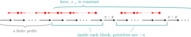
Figure 2: The run in $\mathcal{B}$ (in black), and the order in which the $s_{i}$’s are computed (in red).

For $i$’s as in the second item, it follows from Lemma B.4 that $(q_{i},m_{i},s_{i})\xrightarrow{c_{i}}(q_{i+1},m_{i+1},s_{i+1})$, and moreover, assuming $i\geq i_{0}$, that $(s_{i})_{<x}=(s_{i+1})_{<x}$. Thus for all $i\geq i_{0}$ we have $(s_{i})_{<x}=s_{<x}$ hence we also have, by Lemma B.6, that $(q_{i},m_{i},s_{i})\xrightarrow{c_{i}}(q_{i+1},m_{i+1},s_{i+1})\text{ in }\overline{G}$ for $i$’s as in the first item.

inline,size=,backgroundcolor=pink]todo: figure - Pierre

Appendix C Proof of Theorem 4.1 (Generalised Kopczyński’s conjecture)

We let $\mathcal{A}^{\varepsilon}$ be the automaton defined in Section 4 (i.e. a version of the cascade product of $\mathcal{A}_{1}^{\varepsilon}\times\mathcal{A}_{2}^{\varepsilon}$ with $\mathcal{T}$). In this appendix we prove: See 4.11

First, we need a few remarks on the structure of $\varepsilon$-complete automata. We write $q\xleftrightarrow{\varepsilon:x+1}q^{\prime}$ to denote the conjunction of $q\xrightarrow{\varepsilon:x+1}q^{\prime}$ and $q^{\prime}\xrightarrow{\varepsilon:x+1}q$. Given two states $q,q^{\prime}$ in the same part of a $k$-wise $\varepsilon$-complete automaton, we call breakpoint priority of $q$ and $q^{\prime}$ the least even $x^{(0)}$ such that $q\xleftrightarrow{\varepsilon:x^{(0)}+1}q^{\prime}$ does not hold. Note that this is a property of the unordered pair $\{q,q^{\prime}\}$. Observe also that by the definition of $\varepsilon$-completeness, we have either $q\xrightarrow{\varepsilon:x^{(0)}}q^{\prime}$ or $q^{\prime}\xrightarrow{\varepsilon:x^{(0)}}q$. Moreover, assuming that $q\xrightarrow{\varepsilon:x^{(0)}}q^{\prime}$, we also get that there can be no $q^{\prime}\xrightarrow{\varepsilon:x}q$, for even $x$, otherwise we would accept some run labelled by $\Sigma^{*}\varepsilon^{\omega}$; therefore for even $x\geq x^{(0)}$ we also have $q\xrightarrow{\varepsilon:x}q^{\prime}$. To sum up, if $x^{(0)}$ is the breakpoint priority of $\{q,q^{\prime}\}$ and $q\xrightarrow{\varepsilon:x^{(0)}}q^{\prime}$, then:

• $q\xleftrightarrow{\varepsilon:y}q^{\prime}$ for all odd $y<x^{(0)}$;

• $q\xrightarrow{\varepsilon:x}q^{\prime}$ for all $x\geq x^{(0)}$; and

• there is no transition $q^{\prime}\xrightarrow{\varepsilon:x}q$ for even $x$.

Finally, observe that in $\mathcal{A}_{2}^{\varepsilon}$, since there are no transitions with priority $0$ (and therefore $\xrightarrow{\varepsilon:1}$ connects every ordered pair of states), breakpoint priorities are always $\geq 2$.

We are now ready to prove Lemma 4.11

Proof C.1 (Proof of Lemma 4.11).

First observe that the $k_{1}$ parts of $\mathcal{A}_{1}^{\varepsilon}$ and the $k_{2}$ parts of $\mathcal{A}_{2}^{\varepsilon}$ naturally induce a partition of the states of $\mathcal{A}^{\varepsilon}$ into $k_{1}k_{2}$ parts. Let $r=(q_{1},q_{2},\tau)$ and $r^{\prime}=(q^{\prime}_{1},q^{\prime}_{2},\tau^{\prime})$ be two states in the same part of $\mathcal{A}^{\varepsilon}$, that is, $q_{l}$ and $q^{\prime}_{l}$ are in the same part in $\mathcal{A}_{l}^{\varepsilon}$, for $l=1,2$. We will show that for some even output priority $x^{(0)}$, it holds that:

1. $r\xleftrightarrow{\varepsilon:x^{(0)}-1}r^{\prime}$; and

2. either $r\xrightarrow{\varepsilon:x^{(0)}}r^{\prime}$ or $r^{\prime}\xrightarrow{\varepsilon:x^{(0)}}r$.

Note that since $r\xrightarrow{\varepsilon:t}r^{\prime}$ in $\mathcal{A}^{\varepsilon}$ implies $r\xrightarrow{\varepsilon:t^{\prime}}r^{\prime}$ for all $t^{\prime}\preccurlyeq t$, the two points above imply that for every even $x<x^{(0)}$ we have $r\xleftrightarrow{\varepsilon:x+1}r^{\prime}$ and for every even $x\geq x^{(0)}$, either $r\xrightarrow{\varepsilon:x^{(0)}}r^{\prime}$ or $r^{\prime}\xrightarrow{\varepsilon:x^{(0)}}r$. Therefore, this will prove that $\mathcal{A}^{\varepsilon}$ is $(k_{1}k_{2})$-wise $\varepsilon$-complete.

Let $x^{(0)}_{1}$ and $x^{(0)}_{2}$ denote the breakpoint priorities of $\{q_{1},q^{\prime}_{1}\}$, $\{q_{2},q^{\prime}_{2}\}$ in $\mathcal{A}_{1}^{\varepsilon}$ and $\mathcal{A}_{2}^{\varepsilon}$, respectively (even and $\geq 2$). Let $i_{T}$ be the largest index such that $\tau[..i_{T}]=\tau^{\prime}[..i_{T}]$, with $i_{T}=0$ if $\tau[1]\neq\tau^{\prime}[1]$. We distinguish two cases, depending on whether some $x^{(0)}_{l}-1$ appears in $\tau[..i_{T}]$.

a) $i_{T}<\mathsf{ind}_{\tau}(x^{(0)}_{1}),\mathsf{ind}_{\tau}(x^{(0)}_{2})$.

Note that, in particular, $0<x^{(0)}_{1},x^{(0)}_{2}$.

We show that in this case, we can set $x^{(0)}=2i_{T}+2$. We prove the two points above:

• We will find odd priorities $y_{1}$ and $y_{2}$ such that

  $$\underbrace{q_{1}\xrightarrow{\varepsilon:y_{1}}q^{\prime}_{1}}_{\text{ in }\mathcal{A}_{1}}\text{ and }\underbrace{q_{2}\xrightarrow{\varepsilon:y_{2}}q^{\prime}_{2}}_{\text{ in }\mathcal{A}_{2}}\text{ and }\underbrace{\tau\xrightarrow{(y_{1},y_{2}):x^{(0)}-1}\tau^{\prime}}_{\text{ in }\overline{\mathcal{T}}},$$

  which gives the wanted result when applied symmetrically in the other direction. Consider the element $\tau[i_{T}+1]$ (odd), and assume w.l.o.g. that it belongs to $[d_{1}]$. We let $y_{1}=\tau[i_{T}+1]$. Note that $1\leq y_{1}<x^{(0)}_{1}$ , as $i_{T}+1\leq\mathsf{ind}_{\tau}(x^{(0)}_{1})$, and therefore we have $q_{1}\xleftrightarrow{\varepsilon:y_{1}}q^{\prime}_{1}$. We let $y_{2}=x^{(0)}_{2}-1$; by definition of $x^{(0)}_{2}$ we have $q_{2}\xleftrightarrow{\varepsilon:y_{2}}q^{\prime}_{2}$. As $\mathsf{ind}_{\tau}(y_{2})=\mathsf{ind}_{\tau}(x^{(0)}_{2})>\mathsf{ind}_{\tau}(x^{(0)}_{1})$ we have the third wanted transition $\tau\xrightarrow{(y_{1},y_{2}):2i_{T}+1}\tau^{\prime}$ in $\overline{\mathcal{T}}$, as wanted. By flipping $\tau$ and $\tau^{\prime}$ and applying the same reasoning, we get the transition $r^{\prime}\xrightarrow{\varepsilon:x^{(0)}-1}r$, as required (note that we also have $i_{T}<\mathsf{ind}_{\tau^{\prime}}(x^{(0)}_{1}),\mathsf{ind}_{\tau^{\prime}}(x^{(0)}_{2})$ by definition of $i_{T}$).

• We assume w.l.o.g. that $\tau^{\prime}<\tau$. By definition of $i_{T}$, we have that $\tau^{\prime}<_{i_{T}+1}\tau$. Let $z=\tau[i_{T}+1]$ (which belong to $[d_{2}]^{*}_{\mathrm{odd}}$ if $\tau^{\prime}<_{i_{T}+1}\tau$). As $z\leq x^{(0)}_{2}$, we have $q_{2}\xrightarrow{\varepsilon:z}q^{\prime}_{2}$. Also, $q_{1}\xrightarrow{\varepsilon:x^{(0)}_{1}-1}q^{\prime}_{1}$. Using point (3) of the definition of $\overline{\mathcal{T}}$, we have $\tau\xrightarrow{(x^{(0)}_{1}-1,z):2i_{T}+2}\tau^{\prime}$. We conclude that $r\xrightarrow{\varepsilon:x^{(0)}}r^{\prime}$.

b) Either $\mathsf{ind}_{\tau}(x^{(0)}_{1})\leq i_{T}$ or $\mathsf{ind}_{\tau}(x^{(0)}_{2})\leq i_{T}$.

We assume w.l.o.g. that $\mathsf{ind}_{\tau}(x^{(0)}_{1})<\mathsf{ind}_{\tau}(x^{(0)}_{2})$. We let $x^{(0)}=2\mathsf{ind}_{\tau}(x^{(0)}_{1})$; note that $\tau\xrightarrow{(x^{(0)}_{1},x^{(0)}_{2}-1):x^{(0)}}$ and $\tau\xrightarrow{(x^{(0)}_{1}-1,x^{(0)}_{2}-1):x^{(0)}-1}$ in $\mathcal{T}$. We verify the two cases highlighted above.

• We have $q_{l}\xleftrightarrow{\varepsilon:x^{(0)}_{l}-1}q_{l}$ for $l=1,2$. As $\tau[..i_{T}]=\tau^{\prime}[..i_{T}]$, thanks to rule (1) in the definition of $\overline{\mathcal{T}}$, we have $\tau\xleftrightarrow{(x^{(0)}_{1}-1,x^{(0)}_{2}-1):x^{(0)}-1}\tau^{\prime}$, and so we get $r\xleftrightarrow{\varepsilon:x^{(0)}-1}r^{\prime}$, as required.

• We have one of the transitions $q_{1}\xrightarrow{\varepsilon:x^{(0)}_{1}}q_{1}^{\prime}$ or $q_{1}^{\prime}\xrightarrow{\varepsilon:x^{(0)}_{1}}q_{1}$; assume we are in the first case. Since $q_{2}\xleftrightarrow{\varepsilon:x^{(0)}_{2}-1}q^{\prime}_{2}$, we also have $\tau\xrightarrow{(x^{(0)}_{1},x^{(0)}_{2}-1):x}\tau^{\prime}$, so we conclude that $r\xrightarrow{\varepsilon:x}r^{\prime}$.

This concludes the proof of Theorem 4.1.

Appendix D Proof of Proposition 5.3 (No 1-to-2 player lift)

See 5.3

Proof D.1.

We show that in every game with objective $W_{n}$ and all vertices controlled by Eve, if she can win, she has a winning strategy with memory $2$. Let $G$ be such a game. By prefix-independence of $W_{n}$, we can assume that Eve wins no matter what is the initial vertex of $G$. For each vertex $v\in V(G)$, we let $\chi_{1}(v)$ be the smallest element in $\SS_{n}$ such that there is a path starting in $v$ that produces a colour $c$, and we fix one such finite path $\pi_{v}^{1}=v\xrightarrow{uc}v^{\prime}$ of minimal length. We let $\chi_{2}(v)$ be the second smallest such element (which exists, as Eve wins the game), and fix a finite path $\pi_{v}^{2}$ of minimal length producing it. Note that if $v\xrightarrow{u}v^{\prime}$ is a path in $G$, then $\chi_{1}(v)\leq\chi_{1}(v^{\prime})$.

We define a $2$-memory strategy for Eve as follows: when in a vertex $v$ and memory state $1$, she will take the first edge from $\pi_{v}^{1}$. If this edge has colour $\chi_{1}(v)$, we update the memory state to $2$, and keep it $1$ on the contrary. When in the memory state $2$, she will take the first edge from $\pi_{v}^{1}$, and update the memory state to $1$ if and only if this edge has colour $\chi_{2}(v)$.

We show that this strategy ensures the objective $W$. Let $v_{0}\xrightarrow{c_{1}}v_{1}\xrightarrow{c_{2}}\dots$ be an infinite play consistent with this strategy. Let $a=\limsup\chi_{1}(v_{i})$. We claim that we produce both $a$ and a colour $>a$ infinitely often. Let $i_{0}$ be large enough so that $\chi_{1}(v_{i})>a$ for $i\geq i_{0}$. Note that in this case, if $v_{i}\xrightarrow{u}v_{i^{\prime}}$ is a path that does not contain colour $\chi_{2}(v_{i})$, then $\chi_{2}(v_{i^{\prime}})=\chi_{2}(v_{i})$. If in step $i$ we are in memory state $1$, in exactly $|\pi_{v_{i}}^{1}|$ steps we will produce output $\chi_{1}(v_{i})$ and change the memory state to $2$. Likewise, by the remark above, if we are in the memory state $2$, in $|\pi_{v_{i}}^{2}|$ steps we will produce $\chi_{2}(v_{i})>a$ and change to the memory state $1$. This concludes the proof.

References

- [1] Udi Boker and Karoliina Lehtinen. When a little nondeterminism goes a long way: An introduction to history-determinism. ACM SIGLOG News, 10(1):24–51, 2023. doi:10.1145/3584676.3584682.
- [2] Patricia Bouyer, Antonio Casares, Mickael Randour, and Pierre Vandenhove. Half-positional objectives recognized by deterministic Büchi automata. Log. Methods Comput. Sci., 20(3), 2024. doi:10.46298/LMCS-20(3:19)2024.
- [3] Patricia Bouyer, Nathanaël Fijalkow, Mickael Randour, and Pierre Vandenhove. How to play optimally for regular objectives? In ICALP, volume 261 of LIPIcs, pages 118:1–118:18, 2023. doi:10.4230/LIPIcs.ICALP.2023.118.
- [4] Patricia Bouyer, Mickael Randour, and Pierre Vandenhove. Characterizing omega-regularity through finite-memory determinacy of games on infinite graphs. TheoretiCS, 2, 2023. doi:10.46298/THEORETICS.23.1.
- [5] Patricia Bouyer, Stéphane Le Roux, Youssouf Oualhadj, Mickael Randour, and Pierre Vandenhove. Games where you can play optimally with arena-independent finite memory. Log. Methods Comput. Sci., 18(1), 2022. doi:10.46298/LMCS-18(1:11)2022.
- [6] J. Richard Büchi and Lawrence H. Landweber. Solving sequential conditions by finite-state strategies. Transactions of the American Mathematical Society, 138:295–311, 1969. URL: http://www.jstor.org/stable/1994916.
- [7] Antonio Casares. On the minimisation of transition-based Rabin automata and the chromatic memory requirements of Muller conditions. In CSL, volume 216, pages 12:1–12:17, 2022. doi:10.4230/LIPIcs.CSL.2022.12.
- [8] Antonio Casares and Pierre Ohlmann. Positional -regular languages. In LICS, pages 21:1–21:14. ACM, 2024. doi:10.1145/3661814.3662087.
- [9] Antonio Casares and Pierre Ohlmann. Positional -regular languages. CoRR, abs/2401.15384, 2024. doi:10.48550/ARXIV.2401.15384.
- [10] Antonio Casares and Pierre Ohlmann. Characterising memory in infinite games. Log. Methods Comput. Sci., 2025. To appear. URL: https://doi.org/10.48550/arXiv.2209.12044.
- [11] Edmund M. Clarke, I. A. Draghicescu, and Robert P. Kurshan. A unified approch for showing language inclusion and equivalence between various types of omega-automata. Inf. Process. Lett., 46(6):301–308, 1993. doi:10.1016/0020-0190(93)90069-L.
- [12] Edmund M. Clarke, Thomas A. Henzinger, Helmut Veith, and Roderick Bloem, editors. Handbook of Model Checking. Springer, Cham, 2018. doi:10.1007/978-3-319-10575-8_2.
- [13] Thomas Colcombet, Nathanaël Fijalkow, and Florian Horn. Playing safe. In FSTTCS, volume 29 of LIPIcs, pages 379–390, 2014. doi:10.4230/LIPIcs.FSTTCS.2014.379.
- [14] Thomas Colcombet and Damian Niwiński. On the positional determinacy of edge-labeled games. Theor. Comput. Sci., 352(1-3):190–196, 2006. doi:10.1016/j.tcs.2005.10.046.
- [15] Stefan Dziembowski, Marcin Jurdziński, and Igor Walukiewicz. How much memory is needed to win infinite games? In LICS, pages 99–110, 1997. doi:10.1109/LICS.1997.614939.
- [16] Olivier Finkel, Michał Skrzypczak, Ryszard Janicki, Slawomir Lasota, and Natalia Sidorova. On the expressive power of non-deterministic and unambiguous petri nets over infinite words. Fundamenta Informaticae, 183(3-4):243–291, 2022. doi:10.3233/FI-2021-2088.
- [17] Hugo Gimbert and Edon Kelmendi. Submixing and shift-invariant stochastic games, 2022. Version 2. URL: https://arxiv.org/abs/1401.6575v2.
- [18] Hugo Gimbert and Wieslaw Zielonka. Games where you can play optimally without any memory. In CONCUR, volume 3653, pages 428–442, 2005. doi:10.1007/11539452_33.
- [19] Yuri Gurevich and Leo Harrington. Trees, automata, and games. In STOC, pages 60–65, 1982. doi:10.1145/800070.802177.
- [20] Eryk Kopczyński. Half-positional Determinacy of Infinite Games. PhD thesis, University of Warsaw, 2008.
- [21] Alexander Kozachinskiy. Energy games over totally ordered groups. In CSL, volume 288 of LIPIcs, pages 34:1–34:12, 2024. doi:10.4230/LIPICS.CSL.2024.34.
- [22] Pierre Ohlmann. Monotonic graphs for parity and mean-payoff games. (Graphes monotones pour jeux de parité et à paiement moyen). PhD thesis, Université Paris Cité, France, 2021. URL: https://tel.archives-ouvertes.fr/tel-03771185.
- [23] Pierre Ohlmann. Characterizing positionality in games of infinite duration over infinite graphs. TheoretiCS, Volume 2, January 2023. doi:10.46298/theoretics.23.3.
- [24] Pierre Ohlmann and Michal Skrzypczak. Positionality in and a completeness result. In STACS, volume 289, pages 54:1–54:18, 2024. doi:10.4230/LIPICS.STACS.2024.54.
- [25] Michal Skrzypczak. Topological extension of parity automata. Inf. Comput., 228:16–27, 2013. doi:10.1016/J.IC.2013.06.004.
- [26] Robert S. Streett and E. Allen Emerson. An automata theoretic decision procedure for the propositional mu-calculus. Inf. Comput., 81(3):249–264, 1989. doi:10.1016/0890-5401(89)90031-X.
- [27] Pierre Vandenhove. Strategy complexity of zero-sum games on graphs. (Complexité des stratégies des jeux sur graphes à somme nulle). PhD thesis, University of Mons, Belgium, 2023. URL: https://tel.archives-ouvertes.fr/tel-04095220.
- [28] Igor Walukiewicz. Pushdown processes: Games and model checking. In CAV, volume 1102 of Lecture Notes in Computer Science, pages 62–74, 1996. doi:10.1007/3-540-61474-5_58.