Contrastive Representation Distillation via Multi-Scale Feature Decoupling

Abstract

Knowledge distillation is a technique aimed at enhancing the performance of a smaller student network without increasing its parameter size by transferring knowledge from a larger, pre-trained teacher network. Previous approaches have predominantly focused on distilling global feature information while overlooking the importance of disentangling the diverse types of information embedded within different regions of the feature. In this work, we introduce multi-scale decoupling in the feature transfer process for the first time, where the decoupled local features are individually processed and integrated with contrastive learning. Moreover, compared to previous contrastive learning-based distillation methods, our approach not only reduces computational costs but also enhances efficiency, enabling performance improvements for the student network using only single-batch samples. Extensive evaluations on CIFAR-100 and ImageNet demonstrate our method’s superiority, with some student networks distilled using our method even surpassing the performance of their pre-trained teacher networks. These results underscore the effectiveness of our approach in enabling student networks to thoroughly absorb knowledge from teacher networks.

1 Introduction

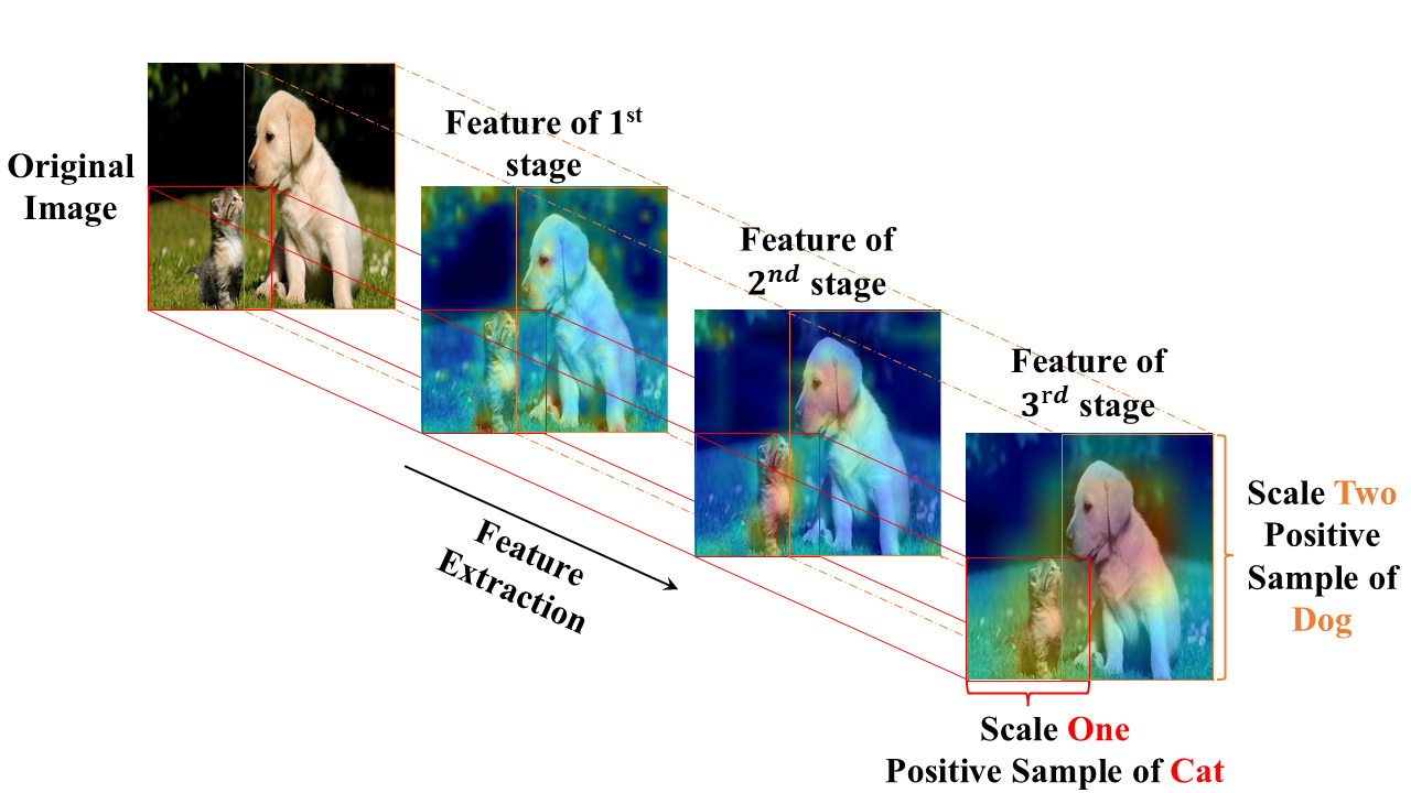
Figure 1: Different Level Feature Heat Map Visualization. Features of different scales and positions focus on distinct category information.

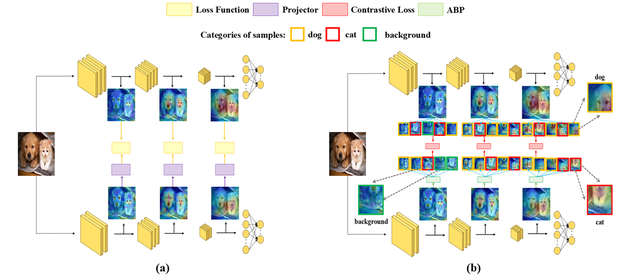
Figure 2: The architectural comparison between our method and traditional distillation methods. (a) Traditional multi-layer feature distillation framework. For single-layer feature distillation, the process involves performing feature distillation at a single stage only. (b) Our proposed method framework, where the features at each layer are decoupled by multiple scales. Different local features focus on different class information. Additionally, we use ABP to enhance the focused feature information, classifying the different feature samples and outputting them into CL (contrastive loss).

The past few decades have witnessed remarkable achievements of neural networks in the field of computer vision. With the proposal of the residual network architecture  (He et al., 2016), the depth of neural networks has increased significantly. Deeper networks with more parameters have brought improved performance; however, they also come with trade-offs. As network depth increases, both computational and storage costs escalate accordingly, posing a significant challenge to deployment on resource-constrained devices. To address this issue, various model compression techniques have been proposed, including model pruning (Frankle & Carbin, 2018; Li et al., 2016; Liu et al., 2018; Luo et al., 2017), model quantization (Jacob et al., 2018; Courbariaux et al., 2015), lightweight network design (Howard, 2017; Sandler et al., 2018; Zhang et al., 2018), and knowledge distillation (Hinton, 2015; Zagoruyko & Komodakis, 2016; Romero et al., 2014).

In light of the significant potential of knowledge distillation for model compression, we focus on the application and optimization of knowledge distillation techniques in this paper. Knowledge distillation is a specialized form of transfer learning, where the ”knowledge” from a larger pre-trained network (also known as the teacher) is transferred to a smaller student network (a.k.a. the student) to enhance the performance of the latter. Hinton et al. (Hinton, 2015) first propose distilling a teacher’s knowledge into a student by minimizing the Kullback-Leibler (KL) divergence between their predictions. However, logit-based KD approaches fail to fully utilize the ”knowledge” embedded in the teacher network. To address this limitation, FitNet (Romero et al., 2014) introduces distillation using intermediate-layer features of the network. AT (Zagoruyko & Komodakis, 2016) further leverages attention maps to facilitate knowledge transfer. CRD (Tian et al., 2019) improves feature distillation by incorporating contrastive learning for knowledge transfer. Reviewing existing methods based on feature distillation, these approaches essentially achieve knowledge transfer on features by applying certain transformations on the features of each layer or through elaborate design of loss functions. Despite yielding favorable outcomes, these methods remain suboptimal as they primarily focus on transferring global features and do not adequately address the local information within each layer’s features or conduct corresponding processing. As shown in Figure 1, the features at different stages within the network may include information from multiple categories. Consequently, local features at different positions and scales may predominantly focus on distinct category information. Zhang et al. (Zhang et al., 2022) have shown that the process of knowledge distillation primarily emphasizes the transfer of foreground ”knowledge points,” while feature information from different categories, considered as background ”knowledge points,” is often overlooked during the distillation process. Consequently, when only global features are considered as a whole for distillation, the student network may fail to capture the local information in the teacher network fully. This can result in the student being unable to fully assimilate the knowledge from the teacher, leading to suboptimal performance.

To address this issue, we propose a method of feature multi-scale decoupling, we propose a method of multi-scale feature decoupling that decouples the features of the student and teacher networks across multiple scales during the feature distillation process. Decoupling is an effective approach for addressing scenarios where factors of varying importance are sub-optimally treated as a unified whole (Chen et al., 2024). This method ensures that the student not only learns the global feature knowledge from the teacher network but also fully captures the local knowledge.

Additionally, we propose an improved and budget-saving feature distillation method based on contrastive learning. CRD (Tian et al., 2019) requires complex sample processing and a large memory buffer to store feature representations of all samples from both the teacher and student networks, along with additional parameters. By introducing multi-scale feature decoupling to contrastive representation distillation, we not only enrich the number of samples, enabling us to acquire abundant feature information with merely a single batch of samples, but also process global and local features separately. This enables features from different-category samples within the same batch to be treated as negative samples, while even distinct local parts of the same sample, belonging to different categories, are also considered negative samples. Furthermore, the feature multi-scale decoupling process is parameter-free and significantly enriches the sample information. Eventually, the rich and decoupled feature sample information is input into our designed contrastive loss function(CL), leading to enhanced performance of the student network. We also employ the Attention-Based Projector (ABP, detailed in Section 4.2) to enhance discriminative regions through channel-wise attention. The overall framework is shown in Figure 2

In general, we summarize our contributions as follows:

• We reveal the limitations of traditional feature distillation methods that focus solely on global feature information and highlight the resulting issues.

• We propose the multi-scale feature decoupling module and an efficient contrastive representation distillation approach, enriching the feature information using only batch-level inputs and allowing the student network to better acquire feature knowledge from teacher.

• We conduct extensive experiments on several benchmark datasets and achieve state-of-the-art results across multiple teacher-student network pairs, with many students even outperforming their teachers, demonstrating the effectiveness of our method.

2 Related Work

Knowledge distillation transfers the ”dark knowledge” of a complex teacher network to a lightweight student network, enhancing the performance of the student network. Depending on the type of transferred knowledge, previous knowledge distillation (KD) methods can be categorized into three main groups: based on transferring logits (Hinton, 2015; Luo, 2024; Zhao et al., 2022; Sun et al., 2024; Jin et al., 2023; Li et al., 2023), features (Romero et al., 2014; Tian et al., 2019; Chen et al., 2022, 2021; Heo et al., 2019; Park et al., 2019; Ahn et al., 2019), and attention (Zagoruyko & Komodakis, 2016; Guo et al., 2023).

Many transferring features methods followed FitNet (Romero et al., 2014) by utilizing single-stage features for knowledge distillation. PKT (Passalis et al., 2020) aligned the probability distributions of the teacher and student network features by minimizing their statistical divergence. SimKD (Chen et al., 2022) decoupled the classification head from the feature extractor, enabling effective knowledge transfer by directly reusing the teacher’s classifier to guide the student’s feature learning. CRD (Tian et al., 2019) combined contrastive learning with knowledge distillation by leveraging a memory buffer to optimize contrastive objectives.

In the feature-based distillation methods, many works proposed to utilize multi-level feature distillation. OFD (Heo et al., 2019) enhanced student network performance by adjusting the placement of feature distillation layers, introducing a novel activation function called Margin ReLU, and employing partial L2 distance as the feature alignment metric. ReviewKD (Chen et al., 2021) improved knowledge distillation by introducing a review mechanism, in which the lower-layer features of the teacher guide the higher-layer features of the student.

However, previous methods primarily focused on global feature information, without addressing the decoupling of relationships between global and local features. Therefore, we introduce multi-scale decoupling of feature into feature distillation to decouple different levels of knowledge. Furthermore, we improve the previous contrastive representation distillation method. Although also grounded in the mutual information maximization theory, our method eliminates the reliance on a large memory buffer for updating the feature information of positive and negative samples, achieving budget-saving by relying solely on single-batch samples(see Appendix A.1 for detailed analysis). We have also achieved state-of-the-art performance in numerous experiments, further demonstrating the excellence of our method.

3 Method

In Sec. 3.1, we describe the feasibility and implementation of multi-scale feature decoupling. Then in Sec. 3.2, we combine it with a contrastive loss to derive the feature distillation loss function. Finally, the complete training objective is introduced in Sec. 3.3.
Notation. Given a batch of input images $x_{i}$, $x_{j}$ (where $i,j=1,2,...,B$), $i=j$ indicates the same input image. We use $f^{T}$ and $f^{S}$ to denote the feature extractors of the teacher and student networks, respectively. For the penultimate layer features in the feature extractor, we do not apply any processing to the teacher network’s features $f^{T}(x_{j})\in R^{c_{T}\times h_{T}\times w_{T}}$, denoted as $T^{j}$. For the student network’s features $f^{S}(x_{i})\in R^{c_{S}\times h_{S}\times w_{S}}$, we project them using ABP to match the same number of channels as the teacher network, and the resulting features are denoted as $S^{i}$, where $c_{S}$ and $c_{T}$ represent the number of feature channels for the student and teacher networks, respectively. Similarly, $h_{S},w_{S}$ and $h_{T},w_{T}$ are the spatial dimensions of the student and teacher network features, respectively. The classifier of the teacher network, denoted as $fc^{T}$, maps the feature $T^{i}$ to its corresponding class $C^{i}=fc^{T}(T^{i})$.

3.1 Multi-Scale Feature Decoupling

An entire image often couples the information of multiple classes, and during the feature extraction process in neural networks, different stages, scales, and spatial locations of features (referred to as local features) may focus on category-specific information that different from the global features. Therefore, when transmitting the features of each stage, solely transmitting the fused global features of various fine-grained details may lead to ambiguous knowledge transfer to the student network, preventing it from acquiring the knowledge of other category-specific local features within this global feature and resulting in suboptimal performance.

For the multi-scale decoupling module, the main process involves first decoupling the features of each sample from both the teacher and student networks at multiple scales. Afterward, the decoupled feature samples are classified to facilitate the construction of the subsequent contrastive loss function. The specific implementation details are as follows: The feature maps $S^{i}$ and $T^{j}$ obtained from the feature extractors of the student and teacher networks are subjected to pooling operations at multiple scales. As a result, each feature map produces $M$ pooled feature maps with varying pooling sizes and positions, denoted as $S_{m}^{i}\in R^{c_{S}\times 1\times 1},T_{n}^{j}\in R^{c_{T}\times 1\times 1}$, where $m,n=1,2,...,M$, and when $m=n$, it indicates that the pooling size and pooling position of the feature maps are identical. Additionally, when $i=j$, it signifies that the input image to both the student and teacher networks is the same. The feature map $T^{j}$ obtained from the teacher network’s $j$-th input image undergoes multi-scale feature decoupling, resulting in $M$ feature maps $T_{n}^{j}$, which are then fed into the teacher network’s classifier to obtain $M$ categories $C_{n}^{j}=fc^{T}(T_{n}^{j})$. For a batch of input images of size $B$, we obtain $M\times B$ feature samples from both the student and teacher networks. When $C_{m}^{i}=C_{n}^{j}$, where $i=j$ and $m=n$, the corresponding student and teacher feature sample pair $(S_{m}^{i},T_{n}^{j})$ is called a related positive sample pair, where the input image, pooling size, and pooling position are identical; When $C_{m}^{i}=C_{n}^{j}$, where $i\neq j$ or $m\neq n$, it indicates that the corresponding student and teacher feature samples belong to the same category but may differ in input image, pooling size, or pooling position. This pair $(S_{m}^{i},T_{n}^{j})$ is referred to as an other positive sample pair; When $C_{m}^{i}\neq C_{n}^{j}$, it indicates that the corresponding student and teacher feature samples belong to different categories, and we call this pair $(S_{m}^{i},T_{n}^{j})$ a negative sample pair.

3.2 Contrastive Loss

When designing the contrastive loss function, we eliminate the reliance on the large memory buffer used in CRD (Tian et al., 2019), which stores feature information of both teacher and student networks, as well as other parameters. Instead, we enrich the sample data by decoupling the student and teacher features at multiple scales. For a batch of input data with size $B$, we can obtain $B$ pairs of student-teacher network feature maps $(S^{i},T^{i})$. After performing multi-scale decoupling on the features, we can obtain $N=M\times B$ pairs of student-teacher network feature maps $(S_{m}^{i},T_{m}^{i})$.We would like to push closer the representations $S_{m}^{i}$ and $T_{m}^{i}$, while pushing apart $S_{m}^{i}$ and $T_{n}^{j}$ (where $i\neq j$ or $m\neq n$). Specifically, we consider the joint distribution $p(S_{m}^{i},T_{n}^{j})$ between the student network feature samples and the teacher network feature samples, as well as the product of the marginal distributions $p(S_{m}^{i})p(T_{n}^{j})$, in order to maximize the mutual information between related positive sample pairs:

$$I(S_{m}^{i},T_{m}^{i})=E_{p(S_{m}^{i},T_{m}^{i})}(\log(\frac{p(S_{m}^{i},T_{m}^{i})}{p(S_{m}^{i})p(T_{m}^{i})}))$$ (1)

where $E_{p(S_{m}^{i},T_{m}^{i})}(\cdot)$ indicates the expectation over relevant positive sample pairs, $p(S_{m}^{i},T_{m}^{i})$ denotes the joint distribution of relevant positive sample pairs.

To achieve this goal, we defined a distribution $q$ and introduced a latent variable $V$, which determines whether the distribution $q$ for a given pair of student-teacher feature samples $(S_{m}^{i},T_{n}^{j})$ is derived from the joint distribution $p(S_{m}^{i},T_{n}^{j})$ or the product of the marginal distributions $p(S_{m}^{i})p(T_{n}^{j})$:

$$q(S_{m}^{i},T_{n}^{j}|V=1)=p(S_{m}^{i},T_{n}^{j})$$ (2)

$$q(S_{m}^{i},T_{n}^{j}|V=0)=p(S_{m}^{i})p(T_{n}^{j})$$ (3)

When $i=j$ and $m=n$, the student-teacher feature pair is considered as a related positive sample pair. These features originate from the same input image, with identical pooling size and pooling position, making them highly correlated. Thus, we set $V=1$. For the other positive sample pairs introduced in the previous section 3.1, although these samples exhibit certain similarities, they have been effectively decoupled, making them weakly correlated. Consequently, we set $V=0$, and these pairs are filtered out in subsequent operations. For the negative sample pairs, these feature pairs focus on entirely different categories of information. Therefore, we regard them as independent and set $V=0$. The prior probability of the latent variable $T$ can be easily derived as:

$$q(V=1)=\frac{1}{N},q(V=0)=\frac{N-1}{N}$$ (4)

According to Bayes’ theorem, the posterior formula for the variable $V$ can be written as:

$$q(V=1|S_{m}^{i},T_{n}^{j})$$

$$=\frac{q(S_{m}^{i},T_{n}^{j}|V=1)q(V=1)}{q(S_{m}^{i},T_{n}^{j}|V=1)q(V=1)+q(S_{m}^{i},T_{n}^{j}|V=0)q(V=0)}$$

$$=\frac{p(S_{m}^{i},T_{n}^{j})}{p(S_{m}^{i},T_{n}^{j})+(N-1)p(S_{m}^{i})p(T_{n}^{j})}$$ (5)

Taking the negative logarithm of both sides of equation 5, and then applying the monotonicity of the logarithm function, we get:

$$-\log q(V=1|S_{m}^{i},T_{n}^{j})$$

$$=\log(1+\frac{(N-1)p(S_{m}^{i})p(T_{n}^{j})}{p(S_{m}^{i},T_{n}^{j})})$$

$$\geq\log(N-1)-\log(\frac{p(S_{m}^{i},T_{n}^{j})}{p(S_{m}^{i})p(T_{n}^{j})})$$ (6)

To maximize the mutual information between related positive sample pairs, we take the expectation on both sides of equation 6 w.r.t. $q(S_{m}^{i},T_{n}^{j}|V=1)$ (which is equivalent to $p(S_{m}^{i},T_{n}^{j})$, where $i=j$ and $m=n$) After rearranging, we obtain the form of equation 1:

$$I(S_{m}^{i},T_{m}^{i})$$

$$\geq\log(N-1)+E_{p(S_{m}^{i},T_{m}^{i})}(\log q(V=1|S_{m}^{i},T_{n}^{j}))$$ (7)

After removing the constant term on the right-hand side of equation 7, we obtain the lower bound of mutual information between related positive sample pairs, denoted as $MI\ bound$.

$$MI\ bound=E_{p(S_{m}^{i},T_{m}^{i})}(\log q(V=1|S_{m}^{i},T_{n}^{j}))$$ (8)

Maximizing the lower bound $MI\ bound$ is equivalent to maximizing $I(S_{m}^{i},T_{m}^{i})$, but since we cannot obtain the true distribution $q(V=1|S_{m}^{i},T_{n}^{j})$, we construct an approximate distribution $\tilde{q}(V=1|S_{m}^{i},T_{n}^{j})$, the formula is as follows:

$$\tilde{q}(V=1|S_{m}^{i},T_{n}^{j})=\frac{exp(sim(S_{m}^{i},T_{m}^{i}))}{\sum_{j=1}^{B}\sum_{n=1}^{M}D(S_{m}^{i},T_{n}^{j})}$$ (9)

where $sim(\cdot)$ is the cosine similarity function between two feature samples, and $D(S_{m}^{i},T_{n}^{j})$ is a discriminator that determines whether the sample pair belongs to the other positive sample pair:

$$D(S_{m}^{i},T_{n}^{j})=\begin{cases}0,C_{m}^{i}=C_{n}^{j},where\;i\neq j\;or\;m\neq n\\ exp(sim(S_{m}^{i},T_{m}^{j})),otherwise\end{cases}$$ (10)

Therefore, when maximizing Equation 11, it is equivalent to maximizing the mutual information between related positive sample pairs:

$$\max E_{p(S_{m}^{i},T_{m}^{i})}(\log\tilde{q}(V=1|S_{m}^{i},T_{n}^{j}))$$ (11)

Due to the capacity gap, a lightweight student struggles to match the feature magnitude of a cumbersome teacher. Thus, we align the student’s feature distribution with the teacher’s as similar as possible. Therefore, before the feature samples are input into the loss function for calculation, we first perform L2 normalization. The loss function for single-layer feature distillation is as follows:

$$\begin{split}\small&L_{singel\_kd}=\\ &-\frac{1}{BM}\sum_{i=1}^{B}\sum_{m=1}^{M}\frac{exp(sim(Norm(S_{m}^{i}),Norm(T_{m}^{i})))}{\sum_{j=1}^{B}\sum_{n=1}^{M}D(Norm(S_{m}^{i}),Norm(T_{n}^{j}))}\end{split}$$ (12)

where $B$ represents the batch size, $M$ denotes the number of distinct pooled feature maps obtained through multi-scale decoupling of a single feature sample, $Norm(\cdot)$ applies L2 normalization, while $sim(\cdot)$ computes the cosine similarity between two feature samples. $D(\cdot,\cdot)$ as defined in Equation 10, serves as a discriminator to determine whether a student-teacher feature sample pair should be classified as other positive sample pair.

3.3 Training Objective

In the process of feature extraction by neural networks, the focus of feature information varies across stages: shallow features focus on gradient information, middle-layer features capture local information of the target region, and deep-layer features emphasize the global information of the target region. Through experimental studies, we find that different student models have distinct requirements for information at various layers of the teacher network(Details are in Section 4.2). Therefore, when only a single layer is utilized for knowledge distillation, the student network may be unable to effectively learn the knowledge from the teacher network, leading to suboptimal performance. Some student networks may only require knowledge from a single layer of the teacher network to learn effectively, while others may need multiple layers to achieve optimal performance.

In the design of the feature distillation loss function, we carefully consider and decide to apply multi-scale feature decoupling separately to features at each stage, followed by the computation of the contrastive loss as described in Equation 12. Then, the losses from each individual stage are aggregated:

$$L_{kd}=\sum_{Layer}L_{single\_kd}$$ (13)

where $Layer$ refers to all layers from the first stage to the penultimate stage in the feature extraction process. Finally, the distillation loss is combined with the cross-entropy loss $L_{ce}$ from hard labels to obtain the final loss function.

$$L=L_{ce}+\beta L_{kd}$$ (14)

where $\beta$ indicates the hyperparameter, for the trade-off of $L_{ce}$ and $L_{kd}$.

Table 1: The Top-1 Accuracy(%) of different knowledge distillation methods on the validation set of CIFAR-100. The teacher and student have identical architectures but different configurations. The best and second best results are emphasized in bold and underlined cases. We mark the results where our method outperforms the teacher network with *.

Type	Teacher	ResNet110	ResNet110	ResNet56	ResNet32$\times$4	WRN-40-2	WRN-40-2	VGG13
	Acc	74.31	74.31	72.34	79.42	75.61	75.61	74.64
	Student	ResNet32	ResNet20	ResNet20	ResNet8$\times$4	WRN-16-2	WRN-40-1	VGG8
	Acc	71.14	69.06	69.06	72.50	73.26	71.98	70.36
Logit	KD	73.08	70.67	70.66	73.33	74.92	73.54	72.98
	CTKD	73.52	70.99	71.19	73.39	75.45	73.93	73.52
	DKD	74.11	71.06	71.97	76.32	76.24	74.81	74.68
Attention	AT	72.31	70.65	70.55	73.44	74.08	73.93	71.43
	CAT-KD	73.62	71.37	71.37	76.91	75.60	73.93	74.65
Feature	FitNet	71.06	68.99	69.21	73.50	73.58	73.93	71.02
	RKD	71.82	69.25	69.25	71.90	73.35	73.93	71.48
	SimKD	73.92	71.06	71.06	78.08	75.53	73.93	74.89
	OFD	73.23	71.29	71.29	74.95	75.24	73.93	73.95
	ReviewKD	73.89	71.34	71.89	75.63	76.12	73.93	74.84
Feature	CRD	73.48	71.46	71.16	75.48	75.45	73.93	73.94
	Ours	*74.61	72.05	71.46	77.43	*76.66	*75.75	*75.65
	$\uparrow$	+1.13	+0.59	+0.36	+1.95	+1.21	+1.82	+1.71

Table 2: The Top-1 Accuracy(%) of different knowledge distillation methods on the validation set of CIFAR-100. The teacher and student have distinct architectures. The best and second best results are emphasized in bold and underlined cases. We mark the results where our method outperforms the teacher network with *.

Type	Teacher	ResNet32$\times$4	ResNet32$\times$4	ResNet32$\times$4	ResNet32$\times$4	WRN-40-2	VGG13	ResNet50
	Acc	79.42	79.42	79.42	79.42	75.61	74.64	79.34
	Student	ShuffleNetV1	ShuffleNetV2	WRN-40-2	WRN-16-2	ResNet8$\times$4	MobileNetV2	MobileNetV2
	Acc	70.50	71.82	75.61	73.26	72.50	64.60	64.60
Logit	KD	74.07	74.45	77.70	74.90	73.97	67.37	67.35
	CTKD	74.48	75.37	77.66	75.57	74.61	68.50	68.67
	DKD	76.45	77.07	78.46	75.70	75.56	69.71	70.35
Attention	AT	75.55	72.73	77.43	73.91	74.11	59.40	58.58
	CAT-KD	78.26	78.41	78.59	76.97	75.38	69.13	71.36
Feature	FitNet	73.95	73.54	77.69	74.70	74.61	64.16	63.16
	RKD	72.28	73.21	77.82	74.86	75.26	64.52	64.43
	SimKD	77.18	78.39	79.29	77.17	75.29	69.44	69.97
	OFD	75.98	76.82	79.25	76.17	74.36	69.48	69.04
	ReviewKD	77.45	77.78	78.96	76.11	74.34	70.37	69.89
Feature	CRD	75.11	75.65	78.15	75.65	75.24	69.73	69.11
	Ours	78.65	78.67	*80.34	77.48	*76.93	70.47	71.51
	$\uparrow$	+3.54	+3.02	+2.19	+1.83	+1.69	+0.74	+2.40

Table 3: The Top-1 and Top-5 Accuracy(%) on the ImageNet validation set. The best results are emphasized in bold cases.

Teacher/Student	ResNet32/ResNet18		ResNet50/MobileNet
Accuracy	Top-1	Top-5	Top-1	Top-5
Teacher	73.31	91.42	76.16	92.86
Student	69.75	89.07	68.87	88.76
KD	71.03	90.05	70.05	89.80
CTKD	71.38	90.27	71.16	90.11
DKD	71.70	90.41	72.05	91.05
AT	70.69	90.01	69.56	89.33
CAT-KD	71.26	90.45	72.24	91.13
SimKD	71.59	90.48	72.25	90.86
OFD	70.81	89.98	71.25	90.34
ReviewKD	71.61	90.51	72.56	91.00
CRD	71.17	90.13	71.37	90.41
Ours	71.99	90.52	73.06	91.15

Table 4: Ablation study. CL: our designed contrastive loss function. Multi-scale decoupling (MSD) is decomposed into two modules: multi-scale feature pooling (MSP) and sample classification (SC).

CL	MSD		Accuracy
	MSP	SC
			75.48
✓			76.44
✓	✓		77.10
✓	✓	✓	77.43

(a) Vanilla KD

(b) Ours

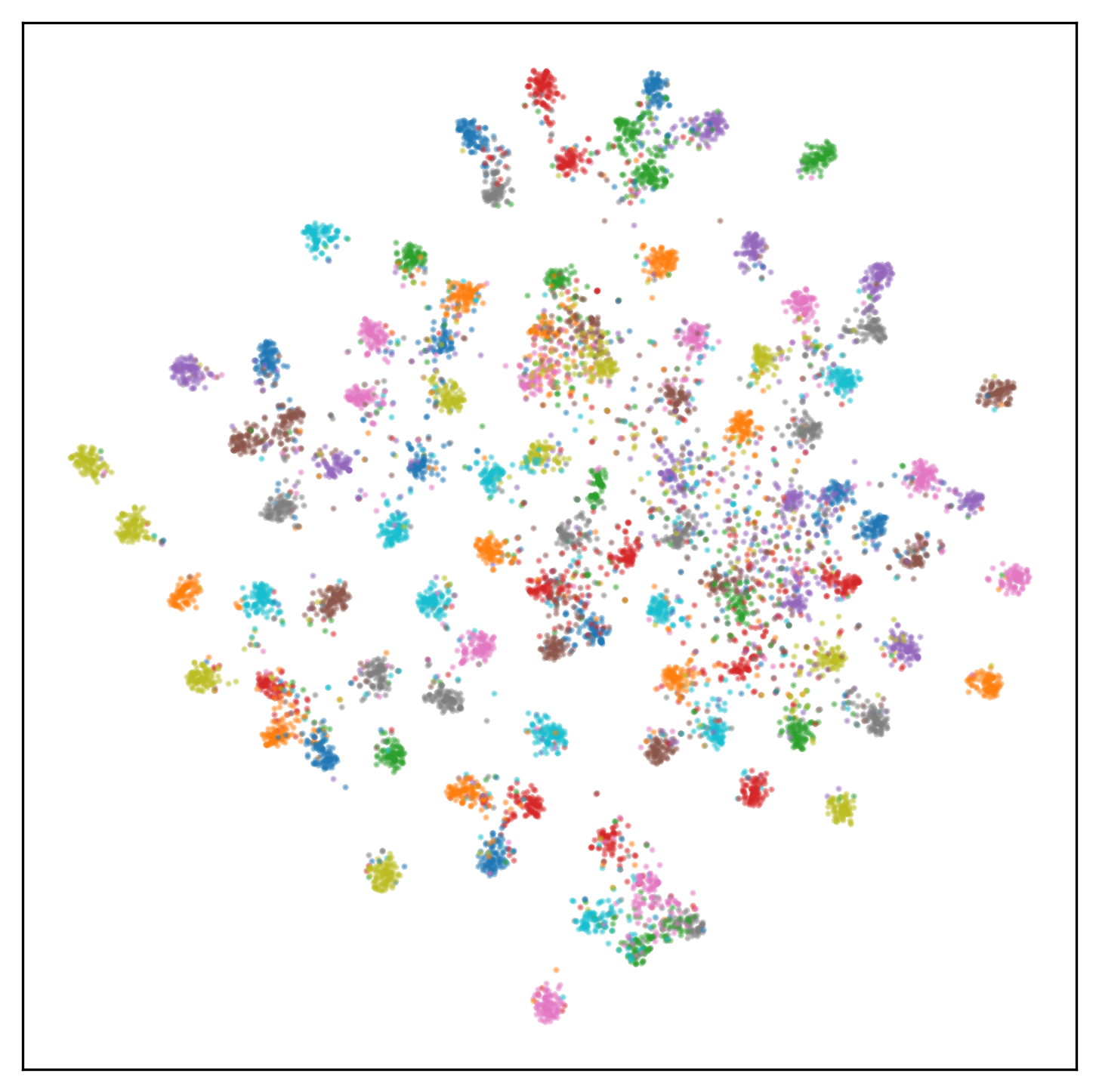
(c) Teacher

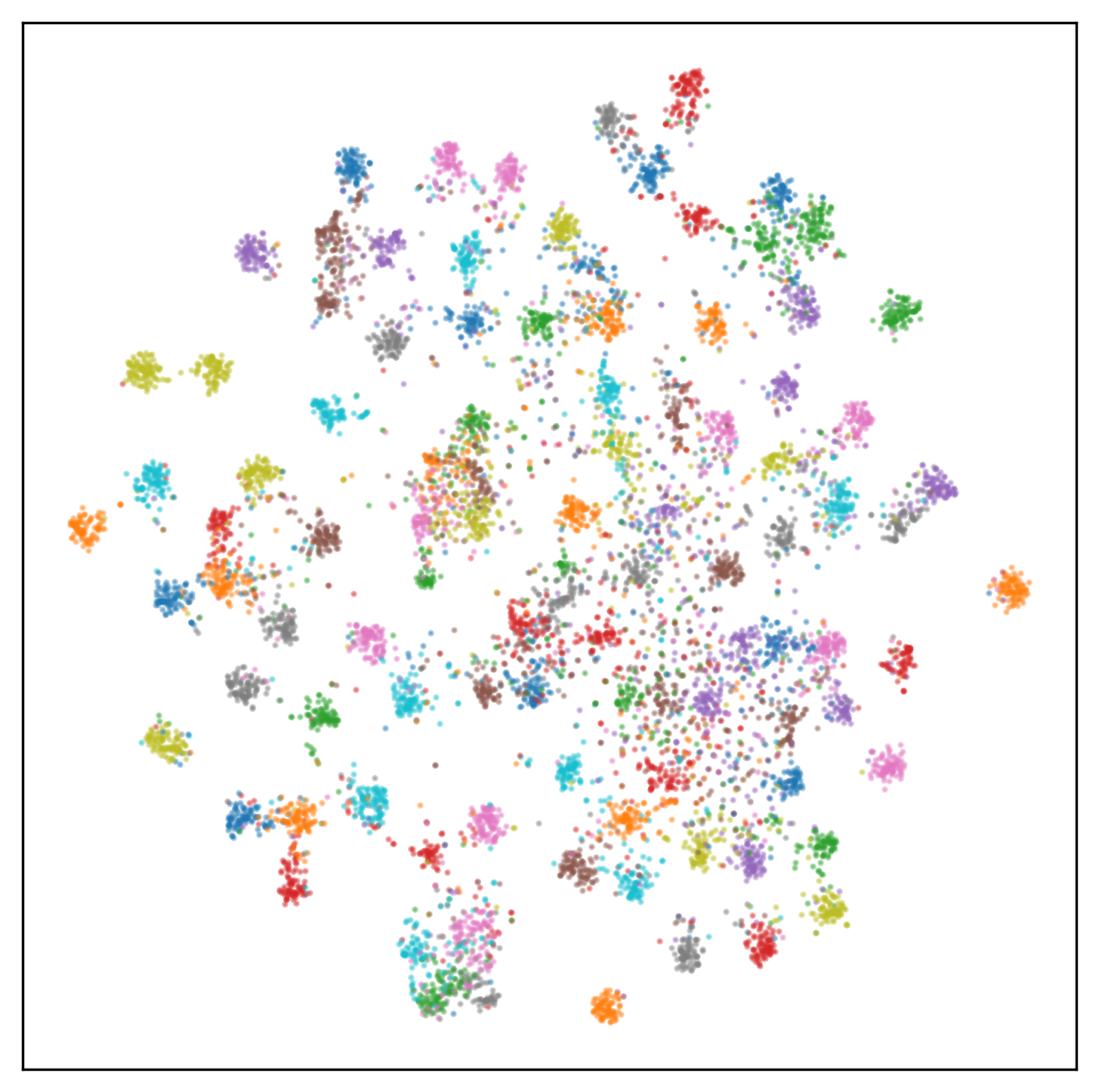
(d) Ours

Figure 3: Visualization results of test images from CIFAR-100 with t-SNE. In (a) and (b), We randomly sample 10 out of the 100 classes. The features extracted by the teacher and student models are represented in dark and light colors, respectively, and in our method, they are nearly indistinguishable. In (c) and (d), we present the visualizations of all classes for the teacher and the student trained with our method.

Table 5: Results of student networks with different projectors. The teacher and student networks used are ResNet32$\times$4 and ResNet8$\times$4,respectively.

Projector	Accuracy(%)
1$\times$1Conv	76.87
1$\times$1Conv-1$\times$1Conv	77.31
1$\times$1Conv-3$\times$3Conv-1$\times$1Conv	77.07
1$\times$1Conv-1$\times$1Conv-Attention	77.43

Table 6: The results of distillation using different levels of information for various student networks.

Feature layers used	ShuffleNetV2	ResNet8x4	WRN-40-2	ShuffleNetV1
$f3$	78.16	77.26	80.81	77.88
$f3,f2$	78.35	77.51	80.57	78.41
$f3,f2,f1$	78.67	77.43	80.34	78.65

4 Experiments

Datasets. Experiments on CIFAR-100 (Krizhevsky et al., 2009) and ImageNet (Russakovsky et al., 2015) are conducted. CIFAR-100 (Krizhevsky et al., 2009) dataset is a well-established benchmark for image classification encompassing 100 categories. It contains 50,000 training images and 10,000 validation images, with each image having a resolution of 32x32 pixels. ImageNet (Russakovsky et al., 2015) is a larger-scale image classification dataset, consisting of images from 1,000 categories. The training set contains 1.28 million images, while the validation set includes 50,000 images.
Implementation Details. On CIFAR-100 dataset, we conduct experiments on various classic network architectures, including VGG (Simonyan, 2014), ResNet (He et al., 2016), WideResNet (Zagoruyko, 2016), MobileNet (Sandler et al., 2018), and ShuffleNet (Ma et al., 2018; Zhang et al., 2018). We use the same training setting of  (Tian et al., 2019).
Specifically, we set 240 epochs to train all models, with the learning rate decaying by a factor of 0.1 every 30 epochs after the first 150 epochs. we set $\beta$ to 0.8. For each model, we set the batch size to 64. Each model is trained three times, and the average accuracy is reported. For fairness, previous method results are either taken from their original papers (when the training settings match ours) or obtained using the authors’ released code with our training setting.
On ImageNet, we use the standard training procedure with a total of 100 epochs. The learning rate is decayed every 30 epochs, with an initial learning rate of 0.1, and the batch size for each training batch is set to 256. we also set $\beta$ to 0.8.

4.1 Main Results

Results on CIFAR-100. We divide the previous methods into three groups as described in Section 2. In the logits-based distillation methods, we use the classic KD method as well as the more advanced CTKD and DKD methods. In the attention-based distillation methods, we use AT and CAT-KD. In the feature-based distillation methods, we use several popular and cutting-edge methods.
Table 1 summarizes results on CIFAR-100 with the teacher and student having identical architectures but different configurations.Table 2 shows the results where the teacher and student have distinct architectures. It is clearly shown that our method achieves state-of-the-art results in the vast majority of cases, with all results outperforming the previous contrastive learning-based feature distillation method CRD significantly. Moreover, our method enables many student networks to outperform the teachers. The results above demonstrate the superiority of our method to fully learn the knowledge from the teacher network.
Results on ImageNet. Table 3 compares the differences between different methods in terms of top-1 and top-5 accuracy. We experiment with two settings of distillation from ResNet50 to MobileNet, and from ResNet34 to ResNet18 respectively. The results indicate that our method outperforms all other methods, whether in the architecture of the same style or different architecture. This further demonstrates the robustness of our method’s performance across various teacher-student network pairs in large-scale datasets.
More Analysis. As shown in Table 1 and Table 2, many student networks outperform their respective teacher networks after applying our distillation method. This finding contradicts the previous empirical belief that the student network should merely mimic the distribution of teacher networks as closely as possible. Some studies, such as (Nagarajan et al., 2023), indicate that student networks learn a systematic bias from the teacher network’s distribution. This systematic bias, induced by the regularization effect of knowledge distillation, amplifies high-confidence predictions while suppressing low-confidence ones, which can lead to student networks outperforming teacher networks.

4.2 Extension Experiments

Ablation Study. We conduct ablation experiments by incrementally adding components to measure their individual effects. The results are shown in Table 4, we conduct each experiment three times and report the average accuracy. We use ResNet8$\times$4 as the student network and ResNet32$\times$4 as the teacher network, with CRD serving as our baseline.

First, we introduce our designed contrastive loss function (denoted as CL), which operates using only single-batch samples, and observe a performance improvement over the baseline. To further highlight the superiority of our proposed multi-scale decoupling mechanism, we divide it into two modules: multi-scale feature pooling (MSP) and sample classification (SC). When multi-scale feature pooling (MSP) is introduced, as shown in the third line, the student network achieves better performance. Combining MSP with sample classification (SC) further improves the results, achieving the best performance.

Feature visualizations. As shown in Figure 3(b), the features extracted by the teacher model (dark colors) and the student model distilled using our method (light colors) form tight clusters within the same class and are clearly separated across different classes, while closely aligning with the teacher network’s features.

Figure 3(c) and Figure 3(d) visualize the feature maps of all classes from the pre-trained teacher network and the student network trained with our method, respectively. It is evident that our approach achieves performance comparable to the teacher network.(in fact, the student network trained with our method outperforms the teacher network in actual results) This demonstrates that our method effectively enables the student model to fully learn the knowledge of the teacher network.

Selection of the Projector. In the selection of the projector, we align with the objective of feature distillation, which is to maximally transfer the knowledge from regions of interest to the student network. Therefore, attention maps are used to enhance the features in the regions of interest, facilitating better knowledge transfer. To demonstrate the superiority of our projector, we conducted experimental comparisons using various projectors under the same settings. The results, as shown in Table 4, highlight the superior performance of our attention-based projector (ABP).

Different student models have distinct requirements for information at various layers. During feature extraction, different stages focus on distinct information. Generally, deeper features capture the global characteristics of the target, while shallower features emphasize more localized feature information, with the shallowest layers focusing primarily on gradient details. This can be observed in Figure 1.

We conduct the following experiments to further validate our finding. For fairness, the teacher network is consistently set as ResNet32x4, and features are incrementally accumulated from the penultimate layer of the feature extractor (denoted as $f3$) upwards, adding $f2$ and $f1$ for comparative analysis. Using student networks with different architectures for validation, the results demonstrate that for some student networks, utilizing only the penultimate layer already achieves optimal performance, outperforming multi-layer feature strategies. However, for other student networks, incorporating more layers of features leads to progressively better performance. This result further confirms our finding.

5 Conclusion and Future Work

In this paper, we propose a framework that overcomes the limitation of prior feature distillation methods, which focus solely on global features. A novel approach is proposed that decouples features at multiple scales and integrates them with a newly designed contrastive representation distillation method. Experiments conducted on ImageNet and CIFAR100 indicate that our framework is both efficient and effective, reaching SOTA results under most settings.

For future research, the interrelations among features at different stages could be decoupled based on the findings in this work to further enhance distillation performance.

Appendix A Appendix

A.1 Compression Ratio.

Generally, with other settings remaining the same, fewer training parameters require less computational resources and result in shorter training time. In contrastive learning, achieving performance improvement requires as many negative samples as possible. To accomplish this, CRD introduces a massive memory buffer that stores feature samples from both the student and teacher networks, along with other parameters. However, this also has a notable drawback: it significantly increases both training time and computational resources.
Our method eliminates the need for a memory buffer and enriches samples within a single batch. This parameter-free process significantly reduces both computational resource dependency and training time requirements. Since CRD only distills features from a single layer, we adopt the same strategy by using the loss function from Equation 12. As shown in Table 7, our method significantly reduces the extra parameters compared to CRD(0.32%-12.91%), and the results from each experiment also outperform CRD. Moreover, our method significantly reduces training time. For instance, under the same hardware configuration, it shortens the training time by approximately one hour for the ResNet32$\times$4-ResNet8$\times$4 teacher-student network pair.

Table 7: The extra training parameters and accuracy rates required by CRD and our single-level distillation method, and the final compression ratio are composed of the ratio of the two methods.

Distillation Mechanism	Teacher	ResNet110	ResNet32$\times$4	ResNet32$\times$4	ResNet32$\times$4	ResNet32$\times$4
	Student	ResNet32	ResNet8$\times$4	WRN-40-2	ShuffleNetV1	ShuffleNetV2
CRD	Acc	73.48	75.51	78.15	75.34	75.65
	Params	12816645	12865797	12849413	12955909	12964101
Ours_single	Acc	74.42(↑1.94)	77.22(↑1.71)	80.81(↑2.66)	77.88(↑2.54)	78.16(↑2.51)
	Params	41281	656641	312321	1672961	1286049
Compression Ratio		0.32%	5.10%	2.43%	12.91%	9.92%

References

- Ahn et al. (2019) Ahn, S., Hu, S. X., Damianou, A., Lawrence, N. D., and Dai, Z. Variational information distillation for knowledge transfer. In Proceedings of the IEEE/CVF conference on computer vision and pattern recognition, pp. 9163–9171, 2019.
- Chen et al. (2022) Chen, D., Mei, J.-P., Zhang, H., Wang, C., Feng, Y., and Chen, C. Knowledge distillation with the reused teacher classifier. In Proceedings of the IEEE/CVF conference on computer vision and pattern recognition, pp. 11933–11942, 2022.
- Chen et al. (2021) Chen, P., Liu, S., Zhao, H., and Jia, J. Distilling knowledge via knowledge review. In Proceedings of the IEEE/CVF conference on computer vision and pattern recognition, pp. 5008–5017, 2021.
- Chen et al. (2024) Chen, T., Liu, H., He, T., Chen, Y., Gan, C., Ma, X., Zhong, C., Zhang, Y., Wang, Y., Lin, H., et al. MECD: Unlocking multi-event causal discovery in video reasoning. In The Thirty-eighth Annual Conference on Neural Information Processing Systems, 2024.
- Courbariaux et al. (2015) Courbariaux, M., Bengio, Y., and David, J.-P. Binaryconnect: Training deep neural networks with binary weights during propagations. Advances in neural information processing systems, 28, 2015.
- Frankle & Carbin (2018) Frankle, J. and Carbin, M. The lottery ticket hypothesis: Finding sparse, trainable neural networks. arXiv preprint arXiv:1803.03635, 2018.
- Guo et al. (2023) Guo, Z., Yan, H., Li, H., and Lin, X. Class attention transfer based knowledge distillation. In Proceedings of the IEEE/CVF Conference on Computer Vision and Pattern Recognition, pp. 11868–11877, 2023.
- He et al. (2016) He, K., Zhang, X., Ren, S., and Sun, J. Deep residual learning for image recognition. In Proceedings of the IEEE conference on computer vision and pattern recognition, pp. 770–778, 2016.
- Heo et al. (2019) Heo, B., Kim, J., Yun, S., Park, H., Kwak, N., and Choi, J. Y. A comprehensive overhaul of feature distillation. In Proceedings of the IEEE/CVF international conference on computer vision, pp. 1921–1930, 2019.
- Hinton (2015) Hinton, G. Distilling the knowledge in a neural network. arXiv preprint arXiv:1503.02531, 2015.
- Howard (2017) Howard, A. G. Mobilenets: Efficient convolutional neural networks for mobile vision applications. arXiv preprint arXiv:1704.04861, 2017.
- Jacob et al. (2018) Jacob, B., Kligys, S., Chen, B., Zhu, M., Tang, M., Howard, A., Adam, H., and Kalenichenko, D. Quantization and training of neural networks for efficient integer-arithmetic-only inference. In Proceedings of the IEEE conference on computer vision and pattern recognition, pp. 2704–2713, 2018.
- Jin et al. (2023) Jin, Y., Wang, J., and Lin, D. Multi-level logit distillation. In Proceedings of the IEEE/CVF Conference on Computer Vision and Pattern Recognition, pp. 24276–24285, 2023.
- Krizhevsky et al. (2009) Krizhevsky, A., Hinton, G., et al. Learning multiple layers of features from tiny images. 2009.
- Li et al. (2016) Li, H., Kadav, A., Durdanovic, I., Samet, H., and Graf, H. P. Pruning filters for efficient convnets. arXiv preprint arXiv:1608.08710, 2016.
- Li et al. (2023) Li, Z., Li, X., Yang, L., Zhao, B., Song, R., Luo, L., Li, J., and Yang, J. Curriculum temperature for knowledge distillation. In Proceedings of the AAAI Conference on Artificial Intelligence, volume 37, pp. 1504–1512, 2023.
- Liu et al. (2018) Liu, Z., Sun, M., Zhou, T., Huang, G., and Darrell, T. Rethinking the value of network pruning. arXiv preprint arXiv:1810.05270, 2018.
- Luo et al. (2017) Luo, J.-H., Wu, J., and Lin, W. Thinet: A filter level pruning method for deep neural network compression. In Proceedings of the IEEE international conference on computer vision, pp. 5058–5066, 2017.
- Luo (2024) Luo, S. W. C. L. Y. Scale decoupled distillation. arXiv preprint arXiv:2403.13512, 2024.
- Ma et al. (2018) Ma, N., Zhang, X., Zheng, H.-T., and Sun, J. Shufflenet v2: Practical guidelines for efficient cnn architecture design. In Proceedings of the European conference on computer vision (ECCV), pp. 116–131, 2018.
- Nagarajan et al. (2023) Nagarajan, V., Menon, A. K., Bhojanapalli, S., Mobahi, H., and Kumar, S. On student-teacher deviations in distillation: does it pay to disobey? Advances in Neural Information Processing Systems, 36:5961–6000, 2023.
- Park et al. (2019) Park, W., Kim, D., Lu, Y., and Cho, M. Relational knowledge distillation. In Proceedings of the IEEE/CVF conference on computer vision and pattern recognition, pp. 3967–3976, 2019.
- Passalis et al. (2020) Passalis, N., Tzelepi, M., and Tefas, A. Probabilistic knowledge transfer for lightweight deep representation learning. IEEE Transactions on Neural Networks and Learning Systems, 32(5):2030–2039, 2020.
- Romero et al. (2014) Romero, A., Ballas, N., Kahou, S. E., Chassang, A., Gatta, C., and Bengio, Y. Fitnets: Hints for thin deep nets. arXiv preprint arXiv:1412.6550, 2014.
- Russakovsky et al. (2015) Russakovsky, O., Deng, J., Su, H., Krause, J., Satheesh, S., Ma, S., Huang, Z., Karpathy, A., Khosla, A., Bernstein, M., et al. Imagenet large scale visual recognition challenge. International journal of computer vision, 115:211–252, 2015.
- Sandler et al. (2018) Sandler, M., Howard, A., Zhu, M., Zhmoginov, A., and Chen, L.-C. Mobilenetv2: Inverted residuals and linear bottlenecks. In Proceedings of the IEEE conference on computer vision and pattern recognition, pp. 4510–4520, 2018.
- Simonyan (2014) Simonyan, K. Very deep convolutional networks for large-scale image recognition. arXiv preprint arXiv:1409.1556, 2014.
- Sun et al. (2024) Sun, S., Ren, W., Li, J., Wang, R., and Cao, X. Logit standardization in knowledge distillation. In Proceedings of the IEEE/CVF Conference on Computer Vision and Pattern Recognition, pp. 15731–15740, 2024.
- Tian et al. (2019) Tian, Y., Krishnan, D., and Isola, P. Contrastive representation distillation. arXiv preprint arXiv:1910.10699, 2019.
- Zagoruyko (2016) Zagoruyko, S. Wide residual networks. arXiv preprint arXiv:1605.07146, 2016.
- Zagoruyko & Komodakis (2016) Zagoruyko, S. and Komodakis, N. Paying more attention to attention: Improving the performance of convolutional neural networks via attention transfer. arXiv preprint arXiv:1612.03928, 2016.
- Zhang et al. (2022) Zhang, Q., Cheng, X., Chen, Y., and Rao, Z. Quantifying the knowledge in a dnn to explain knowledge distillation for classification. IEEE Transactions on Pattern Analysis and Machine Intelligence, 45(4):5099–5113, 2022.
- Zhang et al. (2018) Zhang, X., Zhou, X., Lin, M., and Sun, J. Shufflenet: An extremely efficient convolutional neural network for mobile devices. In Proceedings of the IEEE conference on computer vision and pattern recognition, pp. 6848–6856, 2018.
- Zhao et al. (2022) Zhao, B., Cui, Q., Song, R., Qiu, Y., and Liang, J. Decoupled knowledge distillation. In Proceedings of the IEEE/CVF Conference on computer vision and pattern recognition, pp. 11953–11962, 2022.