Thoughts about boosting superconductivity
Abstract
In a superconductor electrons form pairs despite the Coulomb repulsion as a result of an effective attractive interaction mediated by, for example phonons. In the present paper DeGennes’ description of the dynamically screened Coulomb interaction is adopted for the effective interaction. This model is generalized by including the elastic response of the charge-compensating background and the BCS gap equation is solved for the resulting effective electron-electron interaction. It is demonstrated that the superconducting critical temperature becomes strongly enhanced when the material is tuned close to a structural instability.
I Introduction
Jan Zaanen took no interest in boring subjects. Our first conversation in the autumn of 1982 included superconductivity, the Kondo effect and general relativity. Jan and I had just started our Ph D studies with George Sawatzky and we were making mutual introductions in our shared office in the basement of the chemistry building at the University of Groningen. This conversation was the first one of countless scientific discussions and it kicked off a lasting friendship.
One of the major questions that has occupied the generation to which Jan and I belonged, was inspired by the discovery of high temperature superconductivity in the cuprates bednorz1986 . In BCS theory a pairing instability occurs at a critical temperature where . Here is an attractive pairing interaction, is the static bare pair susceptibility and is an appropriately weighted average energy of the phonons involved in the pairing interaction. The conventional approach has been to argue that in the cuprates bosonic degrees of freedom such as phonons, plasmons, spin-fluctuations, loop-currents or excitons mediate a strong attractive pairing interaction. In a series of papers with Jian-Huang She and others, Jan and his coauthors argued she2009 ; she2011 ; yang2011 ; she2013 , that the bare pair susceptibility in the cuprates has properties qualitatively different from standard metals, causing to be very high even when the pairing interaction isn’t stronger than in other superconducting materials. They started from the Ansatz that the bare pair susceptibility of the cuprates has an algebraic temperature dependence and this, they reasoned, causes the pairing instability to occur at relatively high temperatures. This Ansatz was motivated by the results of Ref. marel2003 on the “Planckian” nature of the relaxation time observed in optical experiments resulting from an animated discussion on our way to a meeting in Poland.
The concept that, as a result of coupling to phonons bardeen1955 or other collective degrees of freedom such as spin fluctuations scalapino1986 or loop currents varma2014 , electrons overcome the Coulomb barrier and form pairs, is inherently counter intuitive. The -to my taste- most intuitively appealing explanation of how this works, was given by DeGennes in his textbook on superconductivity degennes1966 and was based on the “jellium model”. It turned out that solving this model is not entirely trivial ginzburg1968 ; kirzhnits1969 ; marel-berthod2024 and a number of questions remain, some of which I will discuss below.
II The jellium model
The interaction process where two electrons are scattered from to can be described by considering the Coulomb interaction and the screening thereof degennes1966 :
| (1) |
where . In the jellium model the potential landscape of the charge-compensating background is flat, so that the energy-momentum relation is . The dielectric function of a system of free electrons in a compressible positively charged background is (see A )
| (2) |
where is the Thomas-Fermi wave vector, is the plasma frequency of the charge-compensating background, is it’s bulk modulus, it’s mass density and is the length scale below which vanishes. For our discussion it is useful to define reduced parameters for the bulk moduli of the charge-compensating background () and of the electrons ()
| (3) | ||||
| (4) |
both of which are dimensionless constants. To obtain the effective interaction in dimensionless form we multiply with the density of states at the Fermi level
| (5) |
The effective interaction in the s-wave channel is then given by
| (6) |
where is the angle between and . The result of this integral in closed form is
| (7) | |||||
| (8) | |||||
| (9) | |||||
| (10) | |||||
where
| (11) |
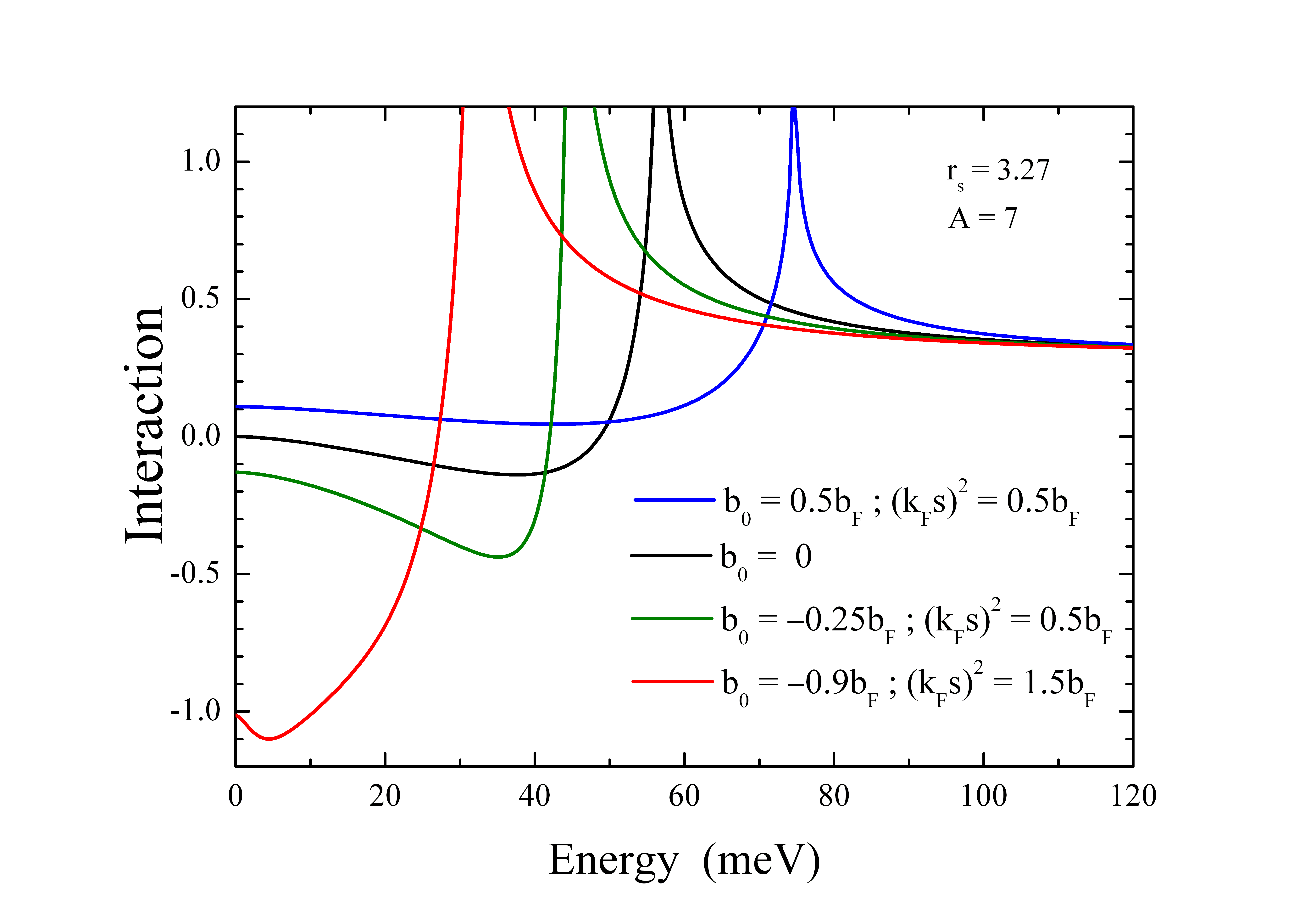
This function is displayed in Fig. 1 for mass number , density cm-3 and a selection of values of and . For the interaction converges to the Thomas-Fermi screened Coulomb repulsion. The interaction has an explicit dependence on momentum and frequency, which is handled in different ways depending on the formalism:
-
1.
If one solves the BCS gap equation bardeen1957 with the Bardeen-Pines approach bardeen1955 , the dependence is treated as the on-shell interaction, .
-
2.
If one solves the Eliashberg equations eliashberg1960 , the dependence on is transformed to Matsubara frequencies which are on the imaginary frequency axis. The singularities seen in Fig. 1 are absent for the imaginary axis, which has certain practical advantages for numerical coding. After solving the gap-function for the Matsubara frequencies one can in principle reconstruct the gap-function along the real axis, which is however a challenging numerical procedure.
-
3.
If one solves the McMillan equation mcmillan1968 , one usually starts from the electron-phonon coupling function which is nowadays typically obtained from a frozen-phonon band structure calculation. Formally the electron-phonon coupling function and the pairing interaction are connected by Kramers-Kronig relations, i.e. , marsiglio2020 where is the the Thomas-Fermi screened Coulomb repulsion. In the MacMillan approach the phonon-mediated interaction is calculated from integrating .
In section IV we will solve the BCS gap equation, i.e. item 1 of the list above. Before doing so we open a parenthesis to briefly discuss a frequently used approximation which we will not use in section IV. This approximation rests on the argument that the most important contribution to the pairing interaction originates from the Fermi surface area. The Coulomb interaction can then be represented by a single parameter , corresponding to
| (12) |
Continuing the discussion of the case , the static () interaction is
| (13) |
which combines the phonon-mediated attraction and the Coulomb repulsion. Correspondingly, the parameter characterizing the phonon-mediated attraction is
| (14) |
We see right away that for we have , for we obtain and for it follows that . Fig. 1 illustrates these three cases. At this point we close the parenthesis about the approximation. In section IV we solve the BCS gap equation with the the substitution and the full and dependence of the interaction.
III Stability considerations
The sound dispersion of a metal is obtained from the condition . Taking the limit , we obtain the sound velocity:
| (15) |
Correspondingly, the overall reduced bulk modulus of the charge-compensating background and the electrons together is
| (16) |
For the overall compressibility is positive. While this is a necessary condition for stability of the system, it is not a sufficient one. A stricter requirement is, that should not be in the range dolgov1981 . Consequently, from the expression for the dielectric function, Eq. 2, for the present model the stability condition is
| (17) |
We furthermore notice that diverges for where
| (18) |
The square root is real for , implying that in this parameter range the system is unstable with respect to a charge density wave (CDW) of wave vector . To evaluate the superconducting properties in this range requires knowledge about the amplitude of the CDW in equilibrium and of its impact on the electron-dispersion, which is outside the limitations of the present model.
IV Superconductivity
The BCS gap equation for s-wave pairing, using the corresponding definition of the interaction, Eq. 6, is
| (19) |
where and is the chemical potential. The density of states is , but note that the factor has been absorbed in the definition of the interaction, Eq. 6. Since in the present study , it follows that . A consequence of Eq. 19 is, that can be chosen real. For display purposes we adopt the convention that is real and positive. As illustrated in Fig. 1, if , the effective interaction has a negative sign for energies well below . On the other hand, , i.e. the static interaction is zero. Given this state of affairs one may wonder if the ground state is superconducting. This question was addressed for the case of hydrogen, also using the jellium model, by Ginzburg and Kirzhnits ginzburg1968 , by Kirzhnits kirzhnits1969 and in a recent paper of the present author and Berthod marel-berthod2024 . The answer was that, in fact, the ground state is superconducting. While the original estimates were in the range of a few 100 K ginzburg1968 ; kirzhnits1969 , we found relatively low values of with this model marel-berthod2024 : The density dependence of is dome shaped with the maximum, K, at . Although this is far below the original estimates ginzburg1968 ; kirzhnits1969 , still the message of principle remains that, despite the fact that , there is a non-trivial superconducting solution. Cohen and Anderson cohen1972 argued that the static dielectric function cannot be negative. Consequently , which is equivalent to the condition . They simplified the interaction potential to for energies below , for energies above and obtained
| (20) |
where is the screened Coulomb pseudopotential. With the aforementioned constraint that the static dielectric function cannot be negative, the additional constraint that , and taking realistic values for the Fermi energy and the phonon plasma frequency ( eV, eV) they concluded that has a maximum of about K. However, as discussed in the previous section, Dolgov, Khirzhnits and Maksimov dolgov1981 have demonstrated that negative values of the static dielectric function are possible, but values in the range cannot occur for a stable system.
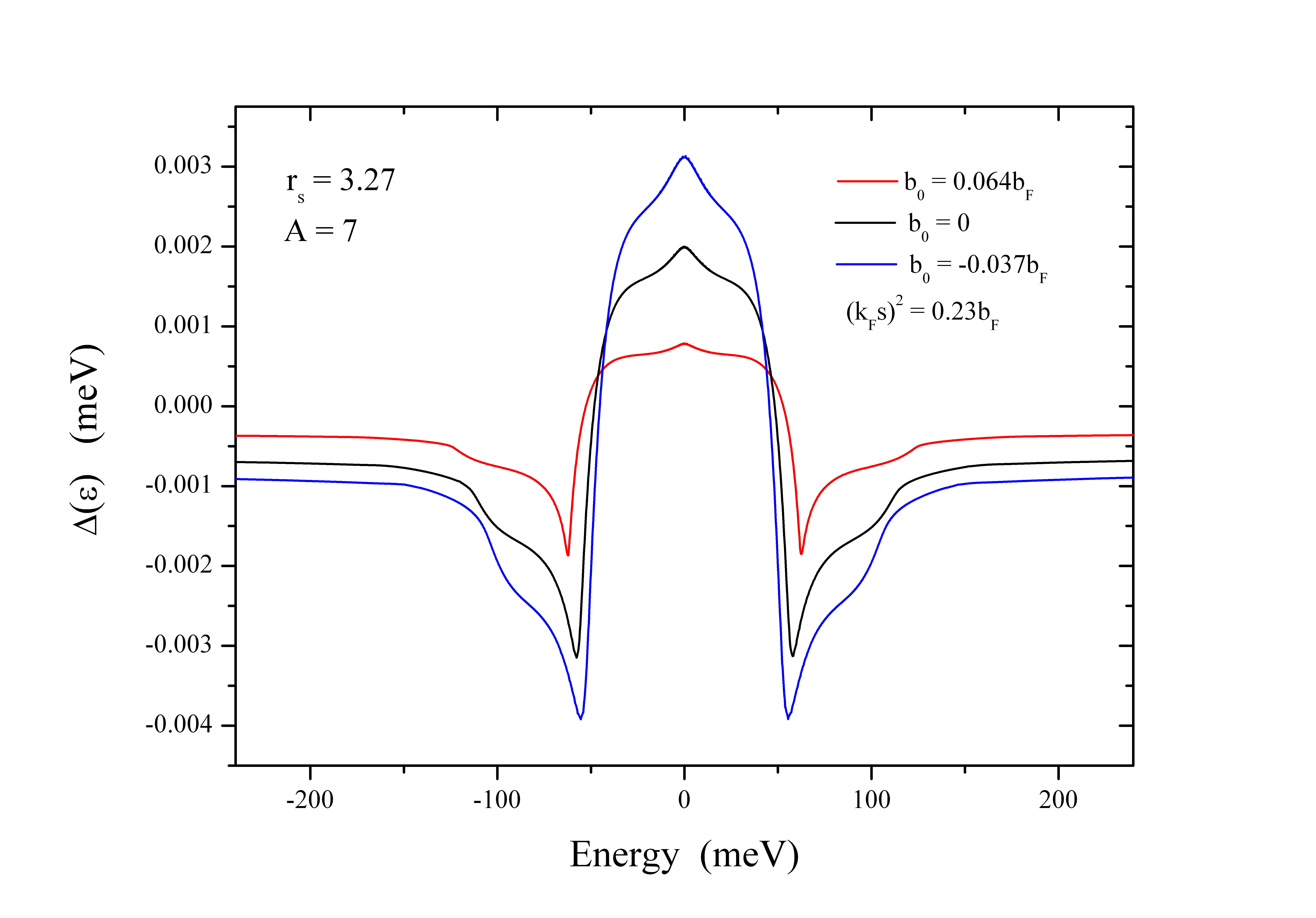
We now turn to the case of lithium. The cell volume of solid lithium is Å3 hanfland1999 . Consequently the conduction-electron density is cm-3 and the Wigner-Seitz radius is . Correspondingly cm-1, eV and meV. In Fig. 2 the gap function is shown for 3 representative cases corresponding to the interaction potential displayed in Fig. 1, positive, zero and negative. We see that the effect of positive is to suppress the superconducting order. In contrast, a negative enhances . Regarding positive it is of interest to point out that in this case the interaction (blue curve in Fig. 1) is entirely repulsive for all energies. Indeed, as illustrated by Eq. 20, even in this case a superconducting solution can be obtained, provided that coleman2015 . In this case the gap changes sign exactly where the Coulomb interaction becomes repulsive as illustrated in Fig. 2 of Ref morel1962 and Fig. 2 of the present paper.
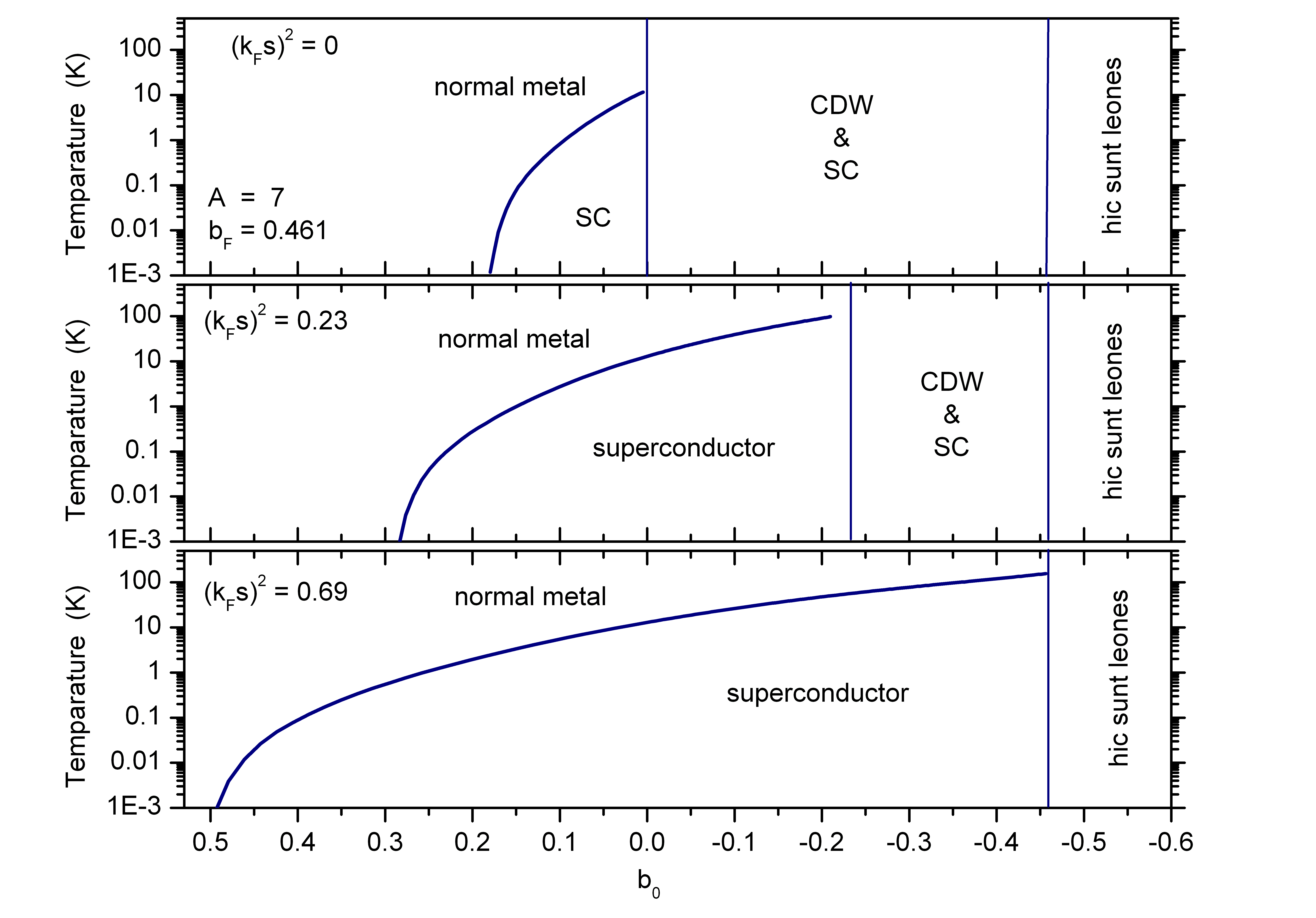
In Ref. marel-berthod2024 , it was shown that where is the condensation energy calculated at , coincides with the critical temperature following from the jump in the specific heat, providing an efficient method for obtaining the critical temperature. In Fig. 3 the critical temperature calculated from the condensation energy is displayed as a function of . Pointing to the left is the direction of positive where the critical temperature decreases below mK. Experimentally, the critical temperature has been determined as mK tuoriniemi2007 . In view of these findings it seems plausible that the low values in the alkali metals are caused by none-negligible elasticity of the charge-compensating background. Pointing to the right is the direction of negative , illustrating that tuning the system toward an elastic instability is a promising strategy for boosting . Note that the acoustic phonons soften in this limit. Using theoretical models different from the one employed here, Bergmann and Rainer bergmann1973 , Maksimov and Savrasov maksimov2001 and Jiang et al. jiang2023 have also concluded that phonon softening should typically be accompanied by an increase of .
While we have seen that a negative is beneficial for superconductivity, the elastic response in this model is given by . If a negative value of were to occur, the material would collapse. For this reason candidates for this type of boosting of superconductivity have to be materials in proximity to a lattice instability, i.e. with while still being in a thermodynamically stable state with . It is tempting to look for a relation to the observed enhancement of lithium up to 20 K for pressures in the range of 20 to 70 GPa shimizu2002 ; deemyad2003 . However, at high densities the overlap of core electrons becomes an important factor and contrary to intuition the electronic structure of lithium becomes less free-electron like neaton1999 , atoms form pairs and above 80 GPa the material is even semiconducting matsuoka2018 . The high pressure phases of lithium are therefore not captured by the model here considered. That said, in a realistic description of the system taking into account the lattice structure, instabilities can occur similar in nature as the one that we discussed above. For the same reason the dielectric function could become negative when the system is tuned close to such an instability, and once again the static interaction would be attractive with the effect of boosting . In that sense, the structural instabilities that are known to occur in lithium under pressure marques2011 , may play a similar role as in the model discussed above.
V Outlook
While we saw that the BCS gap equations can be solved relatively easily for the jellium model, the model itself contains a number of approximations: (i) The Thomas-Fermi approximation was used to describe the screening of the Coulomb interaction. (ii) The frequency dependence of the interaction was treated by substituting the energy difference of the interacting electrons. As was shown by DeGennes degennes1966 this is equivalent to treating the electron-phonon coupling in second order perturbation theory. (iii) The BCS variational wavefunction was assumed. (iv) The potential of the positively charged nuclei was replaced with a constant value. Removing some or all of these approximations would allow for more realistic modeling of the superconducting properties. This may require a radically different approach such as the holographic method holographic of which Jan was a great ambassador. In certain parameter ranges the static susceptibility diverges for wave vector , while the interaction in the s-wave channel of the undistorted system is attractive. Within the limitations of the model used here these aspects could not be addressed more deeply, but I believe that they deserve further attention. Jan Zaanen proposed, together with Jian-Huang She, that high superconductivity can be obtained by using a material for which the pair susceptibility has an algebraic temperature dependence. The main finding of the present paper is that tuning the system close to a lattice instability boosts the pairing interaction. Combining these two elements, algebraic pair susceptibility and proximity to a lattice instability, looks like a promising strategy for the realization of superconductivity at room temperature.
VI Conclusions
We have explored DeGenne’s intuitive “jellium” description of the effective interaction, which treats the Coulomb repulsion and the phonon-mediated interaction in one fell swoop. One additional element -not considered by DeGennes- was included, namely the elastic response of the charge-compensating background. When leaving out this elastic response, the interaction potential vanishes in the static limit. Nevertheless, the BCS gap equation has a solution with a non-zero . If a positive elastic response is added (causing the sound velocity to increase), the interaction potential in the static limit is repulsive. Even in this case can be non-zero. If a negative elastic response is introduced (causing the sound velocity to decrease), the interaction potential in the static limit is attractive and qualitatively similar to the standard BCS scenario for pairing. This has the effect of boosting the critical temperature.
VII Acknowledgements
I am grateful to Erik van Heumen, Christophe Berthod, Louk Rademaker, Frank Marsiglio and Alessio Zaccone for inspiring discussions and comments. This paper is dedicated to the memory of Jan Zaanen who has been an inexhaustible source of original perspectives.
Appendix A Linear response of electrons and a compressible charge-compensating background
The dielectric function is defined as the linear response of the charge of the material to a test charge . The charge of the material has in the present case two contributions: electrons and the massive charge-compensating background. We use the mean-field approximation for the dielectric function, so that it becomes the sum of two independent contributions from the electrons and the charge-compensating background
| (21) |
For the electronic susceptibility we adopt the Thomas-Fermi approximation
| (22) |
The charge-compensating background is characterized by the following properties
-
•
Mass density , charge density with the ratio fixed by the charge/mass ratio of the matter constituting the charge-compensating background, and the corresponding fluctuations of density and current satisfying the continuity relation .
-
•
the bulk modulus , which may depend on the wave vector of the density fluctuation.
is the electric field generated by the test charge and the resulting fluctuation of the charge-compensating background respectively, i.e.
| (23) |
The fluctuations of mass and charge contained inside an infinitesimal volume element are and . The fluctuation of the mass-flow represented by this volume element is . The restoring force due to the density fluctuation is . The acceleration of the mass is given by Newton’s law
| (24) |
so that
| (25) |
Taking the divergence of both sides and using the continuity relation we obtain in the limit of small motion
We substitute and obtain
| (27) |
where
| (28) |
We thus arrive at the contribution to the susceptibility of the massive charge-compensating background
| (29) |
We adopt the following model for the bulkmodulus
| (30) |
where is usually positive, but negative values are possible. One may wonder why a -dependence is introduced. It would in fact be unreasonable to assume that the elastic properties would remain the same at all length scales. The only important requirement for the present discussion is, that converges to zero as , the details of the dependence don’t matter. Substituting Eqs. 22 and 29 in Eq. 2 results in
| (31) |
Data and code availability
-
•
The theoretical data generated in this study are available in Ref. opendataLi . These will be preserved for 10 years. All other data that support the plots within this paper and other findings of this study are available from the author upon reasonable request.
-
•
The custom computer codes used to generate the results reported in this paper are available in Ref. opendataLi .
-
•
Any additional information required to reanalyze the data reported in this paper is available from the author upon request.
Declaration of interests
The author declares no competing interests.
References
- (1) J. G. Bednorz, K. A. Muller, Possible high superconductivity in the Ba-La-Cu-O system, Z. Phys. B: Condens. Matter 64 (1986) 189–193. doi:10.1007/bf01303701.
- (2) J.-H. She, J. Zaanen, BCS superconductivity in quantum critical metals, Phys. Rev. B 80 (2009) 184518. doi:10.1103/PhysRevB.80.184518.
- (3) J.-H. She, B. J. Overbosch, Y.-W. Sun, Y. Liu, K. E. Schalm, J. A. Mydosh, J. Zaanen, Observing the origin of superconductivity in quantum critical metals, Phys. Rev. B 84 (2011) 144527. doi:10.1103/PhysRevB.84.144527.
- (4) S.-X. Yang, H. Fotso, S.-Q. Su, D. Galanakis, E. Khatami, J.-H. She, J. Moreno, J. Zaanen, M. Jarrell, Proximity of the Superconducting Dome and the Quantum Critical Point in the Two-Dimensional Hubbard Model, Phys. Rev. Lett. 106 (2011) 047004. doi:10.1103/PhysRevLett.106.047004.
- (5) J.-H. She, J. Zaanen, Superconductivity and fermionic quantum criticality, Physica C: Superconductivity 493 (2013) 34–35, new3SC-9. doi:https://doi.org/10.1016/j.physc.2013.03.014.
- (6) D. van der Marel, H. J. A. Molegraaf, J. Zaanen, Z. Nussinov, F. Carbone, A. Damascelli, H. Eisaki, M. Greven, P. H. Kes, M. Li, Quantum critical behaviour in a high- superconductor, Nature 425 (2003) 271. doi:10.1038/nature01978.
- (7) J. Bardeen, D. Pines, Electron-Phonon Interaction in Metals, Phys. Rev. 99 (1955) 1140. doi:10.1103/PhysRev.99.1140.
- (8) D. J. Scalapino, E. Loh, J. E. Hirsch, -wave pairing near a spin-density-wave instability, Phys. Rev. B 34 (1986) 8190–8192. doi:10.1103/PhysRevB.34.8190.
- (9) C. M. Varma, Pseudogap in cuprates in the loop-current ordered state, Journal of Physics: Condensed Matter 26 (2014) 505701. doi:10.1088/0953-8984/26/50/505701.
- (10) P. G. De Gennes, Superconductivity of Metals and Alloys, Benjamin, New York, Amsterdam, 1966.
- (11) V. L. Ginzburg, D. A. Kirzhnits, Superconductivity in White Dwarfs and Pulsars, Nature 220 (1968) 148. doi:10.1038/220148b0.
- (12) D. A. Kirzhnits, Superconductivity in Systems with Arbitrary Interaction Sign, ZhETF Pis. Red. 9 (1969) 360.
- (13) D. van der Marel, C. Berthod, Superconductivity in metallic hydrogen, Newton 1 (2025) 100002. doi:10.1016/j.newton.2024.100002.
- (14) J. Bardeen, L. N. Cooper, J. R. Schrieffer, Theory of Superconductivity, Phys. Rev. 108 (1957) 1175. doi:10.1103/PhysRev.108.1175.
- (15) G. M. Eliashberg, Interactions between electrons and lattice vibrations in a superconductor, Sov. Phys. JETP 11.
- (16) W. L. McMillan, Transition Temperature of Strong-Coupled Superconductors, Phys. Rev. 167 (1968) 331. doi:10.1103/PhysRev.167.331.
- (17) F. Marsiglio, Eliashberg theory: A short review, Annals of Physics 417 (2020) 168102, eliashberg theory at 60: Strong-coupling superconductivity and beyond. doi:https://doi.org/10.1016/j.aop.2020.168102.
- (18) O. V. Dolgov, D. A. Kirzhnits, E. Maksimov, On an admissible sign of the static dielectric function of matter, Reviews of Modern Physics 53 (1981) 81. doi:10.1103/RevModPhys.53.81.
- (19) M. L. Cohen, P. W. Anderson, Comments on the Maximum Superconducting Transition Temperature, AIP Conf. Proc. 4 (1972) 17. doi:10.1063/1.2946185.
- (20) M. Hanfland, I. Loa, K. Syassen, U. Schwarz, K. Takemura, Equation of state of lithium to 21 GPa, Solid State Communications 112 (1999) 123. doi:10.1016/S0038-1098(99)00322-1.
- (21) P. Coleman, Introduction to Many-Body Physics, Cambridge University Press, Cambridge. UK. Cambridge, 2015.
- (22) P. Morel, P. W. Anderson, Calculation of the Superconducting State Parameters with Retarded Electron-Phonon Interaction, Phys. Rev. 125 (1962) 1263. doi:10.1103/PhysRev.125.1263.
- (23) J. Tuoriniemi, K. Juntunen-Nurmilaukas, J. Uusvuori, E. Pentti, A. Salmela, A. Sebedash, Superconductivity in lithium below 0.4 millikelvin at ambient pressure, Nature 447 (2007) 187. doi:10.1038/nature05820.
- (24) G. Bergmann, D. Rainer, The sensitivity of the transition temperature to changes in , Z. Phys. 263 (1973) 59–68. doi:10.1007/BF02351862.
- (25) E. Maksimov, D. Savrasov, Lattice stability and superconductivity of the metallic hydrogen at high pressure, Solid State Communications 119 (2001) 569–572. doi:https://doi.org/10.1016/S0038-1098(01)00301-5.
- (26) C. Jiang, E. Beneduce, M. Baggioli, C. Setty, A. Zaccone, Possible enhancement of the superconducting due to sharp Kohn-like soft phonon anomalies, Journal of Physics: Condensed Matter 35 (2023) 164003. doi:10.1088/1361-648X/acbd0a.
- (27) K. Shimizu, H. Ishikawa, D. Takao, T. Yagi, K. Amaya, Superconductivity in compressed lithium at 20 K, Nature 419 (2002) 597. doi:doi.org/10.1038/nature01098.
- (28) S. Deemyad, J. Schilling, Superconducting Phase Diagram of Li Metal in Nearly Hydrostatic Pressures up to 67 GPa, Phys. Rev. Letters 91 (2003) 167001. doi:10.1103/PhysRevLett.91.167001.
- (29) J. B. Neaton, N. W. Ashcroft, Pairing in dense lithium, Nature 400 (1999) 141. doi:10.1038/22067.
- (30) S. Matsuoka, K. Shimizu, Direct observation of a pressure-induced metal-to-semiconductor transition in lithium, Nature 458 (2018) 186. doi:10.1038/nature07827.
- (31) M. Marqués, M. I. McMahon, E. Gregoryanz, M. Hanfland, C. L. Guillaume, C. J. Pickard, G. J. Ackland, R. J. Nelmes, Crystal Structures of Dense Lithium: A Metal-Semiconductor-Metal Transition, Phys. Rev. Lett. 106 (2011) 095502. doi:10.1103/PhysRevLett.106.095502.
- (32) J. Zaanen, Y.-W. Sun, Y. Liu, K. Schalm, Holographic duality in condensed matter physics, Cambridge University Press, 2015.
- (33) D. van der Marel, Open Data to “Thoughts about boosting superconductivity”, Yareta doi:DOI:10.26037/yareta:t4bzvpegabdw5fmyih6faakhba.