A validated fluid-structure interaction simulation model for vortex-induced vibration of a flexible pipe in steady flow

Abstract

We propose a validated fluid-structure interaction simulation framework based on strip methods for the vortex-induced vibration of a flexible pipe. The numerical results are compared with the experimental data from three previous steady flow conditions: uniform, linearly sheared, and bidirectionally sheared flow. The Reynolds number ranges from $10^{4}$ to $10^{5}$. The flow field is simulated via the RANS model, which is based on the open-source software OpenFOAM. The solid field is modeled based on Euler-Bernoulli beam theory, and fluid-structure coupling is implemented via a weak coupling algorithm developed in MATLAB. The vortex-induced vibration response is assessed in terms of amplitude and frequency, along with the differences in strain. Additionally, wavelet analysis and traveling wave phenomena are investigated. The numerical simulation codes and experimental data in this manuscript are openly available, providing a foundation for more complex vortex-induced vibration simulations in the future.

1 Introduction

Vortex-induced vibration (VIV) is a critical phenomenon in offshore engineering, especially for flexible structures such as risers, mooring lines, and pipelines [1]. VIV occurs when fluid flows past these structures, generating a vortex street that induces mechanical oscillations in both the in-line (IL) and cross flow (CF) directions. If not properly considered in the design and operation of these structures, VIV can lead to fatigue damage and structural failure.

The prediction of vortex-induced vibration is a crucial aspect of VIV research, with researchers in both academia and industry having explored this field for nearly half a century. The VIV studies began with bluff cylinders [2, 3]. However, in engineering fields, especially ocean engineering, flexible pipeline structures are widely used. The multi-frequency response and traveling wave characteristics of flexible structures make the VIV response more complex than that of bluff structures. Flexible pipe VIV is a typical fluid-structure interaction (FSI) phenomenon. Therefore, response prediction consists of two parts: the flexible pipe structure model and the flow field model. For the flexible pipe model, Euler-Bernoulli beams with tension and catenary models have been widely validated as effective. With respect to the flow field model, many different low and high fidelity models have been proposed, such as the simple Morison equation and wake oscillator models [4, 5, 6], as well as those based on forced motion hydrodynamic datasets [7, 8, 9] and computational fluid dynamics (CFD). The flow field model plays a crucial role in simulating the VIV phenomenon. Moreover, with the recent development of the submerged floating tunnel, research on coupling schemes, such as weak and strong coupling schemes, has emerged in VIV community.

All VIV response prediction methods for flexible risers must be validated through experiments. However, flexible pipes typically have diameters on the centimeter scale, and their lengths can extend from tens to hundreds of meters [10, 11, 12, 13, 14]. Previous experimental studies focused primarily on the structural response, with a limited focus on the fluid domain. While some studies have attempted to derive hydrodynamic forces on the basis of structural responses [15, 16], there remains a lack of knowledge regarding fluid domain data. Given the important role of viscosity, potential flow theory is insufficient for this purpose. In essence, only CFD methods based on the Navier-Stokes equations can provide meaningful insights into the fluid domain.

For the vortex-induced vibration of flexible risers, high-fidelity three-dimensional DNS simulations are typically limited to Reynolds numbers ($Re$) on the order of hundreds [17, 18, 19, 20]. At these flow speeds, the noise associated with measurement equipment is high, which makes DNS simulations suitable for only purely theoretical research. The slicing method provides a feasible approach for studying high Reynolds numbers. Various CFD strip methods for flexible risers, from Norsk Hydro [21] and VIVIC [22] to Nektar++ [23], have been investigated. However, these methods have two major drawbacks: 1) Flexible riser experiments are extremely costly, making widespread validation of any proposed model difficult. Additionally, the most famous published blind validation was conducted decades ago [24]. 2) The software for these methods is closed-source, which presents a significant barrier to conducting CFD simulations of flexible risers [25].

In this paper, we propose an open-source fluid-structure interaction simulation model for the VIV of a flexible pipe based on the strip method. Validation studies are conducted using three steady flow conditions from previous experimental research. We aim to initiate the open-source development of CFD simulations for flexible pipe VIV. All the experimental data and codes used in this study are hosted on GitHub.

2 Numerical methods

2.1 Fluid domain

The governing equation of the fluid domain is the incompressible Navier-Stokes (N-S) equation, which can be written as:

$$\frac{\partial u_{i}}{\partial x_{i}}=0,$$ (1)

$$\frac{\partial u_{i}}{\partial t}+\frac{\partial u_{i}u_{j}}{\partial x_{j}}=-\frac{1}{\rho}\frac{\partial p}{\partial x_{i}}+\nu\frac{\partial^{2}u_{i}}{\partial x_{j}\partial x_{j}},$$ (2)

where $u_{i}$ represents the fluid velocity, $x_{i}$ represents the coordinates, with the subscript $i=1,2,3$ denoting the $x$, $y$, and $z$ components, $p$ represents the pressure, $\rho$ represents the fluid density, and $\nu$ represents the kinematic viscosity of the fluid.

The above equations serve as the control equations for the fluid domain. Numerical solutions of these equations provide the velocity and pressure distributions within the flow field. However, directly solving these equations requires substantial computational resources, as the grid density is proportional to $Re^{2.6}$[26]. Therefore, the Reynolds-averaged Navier-Stokes (RANS) equations are employed to simplify the solution of the N-S equations. Applying time averaging to the N-S equations yields the following RANS equations:

$$\frac{\partial\bar{u}_{i}}{\partial x_{i}}=0,$$ (3)

$$\frac{\partial\bar{u}_{i}}{\partial t}+\frac{\partial\bar{u}_{i}\bar{u}_{j}}{\partial x_{j}}=-\frac{1}{\rho}\frac{\partial\bar{p}}{\partial x_{i}}+\nu\frac{\partial^{2}\bar{u}_{i}}{\partial x_{j}\partial x_{j}}-\frac{\partial\overline{u_{i}^{\prime}u_{j}^{\prime}}}{\partial x_{j}},$$ (4)

where $\bar{(\cdot)}$ denotes the averaging operator and $\overline{u_{i}^{\prime}u_{j}^{\prime}}$ represents the Reynolds stress, which signifies energy transfer due to turbulent fluctuations. In the RANS equations, the Reynolds stress requires closure modeling, and the SST $k-\omega$ turbulence model [27] is applied for simulation. The open-source partial differential equation solver package based on the finite volume method, OpenFOAM-8 [28], is applied in the present study for simulating the unsteady Reynolds-averaged Navier-Stokes (URANS) equations to obtain the fluid force distribution:

$$\boldsymbol{F}_{f}=\oint(\rho p+\mu\boldsymbol{R}_{dev})dS,$$ (5)

where $\boldsymbol{R}_{dev}$ is the deviatoric Reynolds stress tensor and $\mu$ is the dynamic viscosity. All the time and space schemes of second order. For further details on the numerical schemes, refer to previous studies [29, 30, 31].

2.2 Solid domain

The tensioned flexible pipe undergoing vortex-induced vibration is typically simulated with the Euler-Bernoulli beam model [32, 13]. In this study, the finite element method (FEM) is used to solve for the structural response. The governing equation for the structure is as follows:

$$\boldsymbol{M}\ddot{\boldsymbol{\xi}}+\boldsymbol{C}\dot{\boldsymbol{\xi}}+\boldsymbol{K}\boldsymbol{\xi}=\boldsymbol{F}_{f},$$ (6)

where $\boldsymbol{M}$, $\boldsymbol{C}$, and $\boldsymbol{K}$ are the structural system mass matrix, damping matrix, and stiffness matrix of the structural system, respectively, $\boldsymbol{\xi}$ is the displacement matrix, and $\boldsymbol{F}_{f}$ is the fluid force acting on the structure. More details about the FEM model are provided in A.

The Newmark-$\beta$ method is used to obtain get the time-domain response, with constants $\beta=0.25$ and $\gamma=0.5$. Based on the defined simulation time step $\Delta t$, the following constants are computed:

$$a_{0}=\frac{1}{\beta\Delta t^{2}},\quad a_{1}=\frac{\gamma}{\beta\Delta t},\quad a_{2}=\frac{1}{\beta\Delta t},\quad a_{3}=\frac{1}{2\beta}-1,\quad a_{4}=\frac{\gamma}{\beta}-1,$$ (7)

$$a_{5}=\frac{\Delta t}{2}\left(\frac{\gamma}{\beta}-2\right),\quad a_{6}=\Delta t(1-\gamma),\quad a_{7}=\gamma\Delta t,$$

and the effective stiffness matrix is constructed as:

$$\boldsymbol{K}^{*}=\boldsymbol{K}+a_{0}\boldsymbol{M}+a_{1}\boldsymbol{C},$$ (8)

along with the load vector:

$$\boldsymbol{F}_{t+\Delta t}^{*}=\boldsymbol{F}_{t+\Delta t}+\boldsymbol{M}\left(a_{0}\boldsymbol{\xi}_{t}+a_{2}\dot{\boldsymbol{\xi}}_{t}+a_{3}\ddot{\boldsymbol{\xi}}_{t}\right)+\boldsymbol{C}\left(a_{1}\boldsymbol{\xi}_{t}+a_{4}\dot{\boldsymbol{\xi}}_{t}+a_{5}\ddot{\boldsymbol{\xi}}_{t}\right).$$ (9)

The displacement matrix of the riser at the next time step is obtained via:

$$\boldsymbol{\xi}_{t+\Delta t}=\boldsymbol{K}^{*-1}\boldsymbol{F}_{t+\Delta t}^{*},$$ (10)

$$\dot{\boldsymbol{\xi}}_{t+\Delta t}=\dot{\boldsymbol{\xi}}_{t}+a_{6}\ddot{\boldsymbol{\xi}}_{t}+a_{7}\ddot{\boldsymbol{\xi}}_{t+\Delta t},$$

$$\ddot{\boldsymbol{\xi}}_{t+\Delta t}=a_{0}(\boldsymbol{\xi}_{t+\Delta t}-\boldsymbol{\xi}_{t})-a_{2}\dot{\boldsymbol{\xi}}_{t}-a_{3}\ddot{\boldsymbol{\xi}}_{t}.$$

2.3 Fluid-structural interaction coupling algorithm

VIV is a typical fluid-structure interaction (FSI) phenomenon. Solving fluid-structure interaction problems requires exchanging fluid force information $\boldsymbol{F}_{f}$ and structural displacement information $\boldsymbol{\xi}_{s}$ between the solid and fluid domains. By considering the governing equations in both domains and incorporating boundary conditions at the fluid-structure interface, the fluid-structure coupling governing equations can be expressed as:

$$\left\{\begin{matrix}\begin{aligned} \mathcal{N}(\boldsymbol{u}_{f},p_{f})=0&\qquad\text{in}\quad\Omega_{f},\\ \mathcal{S}(\boldsymbol{\xi}_{s})-\boldsymbol{F}(\boldsymbol{u}_{f},p_{f})=0&\qquad\text{in}\quad\Omega_{s},\\ \boldsymbol{u}_{f}=\boldsymbol{u}_{s}&\qquad\text{on}\quad\Gamma_{f,s},\\ \boldsymbol{\sigma}_{f}=\boldsymbol{\sigma}_{s}&\qquad\text{on}\quad\Gamma_{f,s},\\ \end{aligned}\end{matrix}\right.$$ (11)

where $\mathcal{N}(\cdot)$ represents the fluid domain equations, $\mathcal{S}(\cdot)$ represents the structural domain equations, $\Omega_{f}$ and $\Omega_{s}$ are the fluid and solid domains, respectively, and $\Gamma_{f,s}$ denotes the fluid-structure interface. Fluid-structure coupling solutions typically involve weak or strong coupling approaches. In a weak coupling (or partitioned) approach, the equations for the fluid and solid domains are solved separatelym with a single data exchange step at each coupling step. In a strong coupling, the equations in both domains are solved simultaneously, ensuring the satisfaction of boundary conditions, or separately with multiple data exchange steps.

In the present study, the weak FSI coupling algorithm, as shown in Algorithm 1, solves the fluid and solid equations independently, with a single data exchange at each coupling step. The weak coupling algorithm is applied in this manuscript. In this paper, a weak coupling method is employed for fluid-structure interaction calculations. In contrast, a strong coupling algorithm, which performs multiple iterations within a single time step, is also considered. The differences between the two methods are discussed in 27.

Input: Solid field parameters; Flow field parameters.

Output: Structural response $\boldsymbol{\xi}_{s}$ and flow velocity and pressure field $\boldsymbol{u}_{f},p_{f}$.

1 $t\leftarrow 0$

2while $t<t_{end}$ do

3    $\boldsymbol{F}_{f}$ $\leftarrow$ solve $\mathcal{N}(\boldsymbol{u}_{f},p_{f})=0$

4   $\boldsymbol{\xi}_{s}$ $\leftarrow$ solve $\mathcal{S}(\boldsymbol{u}_{s})-\boldsymbol{F}_{f}=0$

5   Update mesh with $\boldsymbol{\xi}_{s}$

6   $t\leftarrow t+\Delta t$

7 end while

Algorithm 1 Weak coupling algorithm of FSI simulation

3 Benchmark VIV experiments

The benchmark experiments referenced in this manuscript have already been conducted and published by our research group. We only introduced some critical information for the CFD simulation in this manuscript; more details are provided in the references.

3.1 Uniform flow cases

The uniform flow VIV experiment was conducted in the towing tank of the Shanghai Ship and Shipping Research Institute. The flexible riser model was constructed from a brass pipe, coated with a heat-shrink tube to protect the embedded Fiber Bragg Grating (FBG) sensors. This experiment, conducted over a decade ago, utilized a brass riser model with high bending stiffness $EI$, which required high flow velocities to excite higher-mode VIV. As a result, the experimental conditions are not well suited for direct comparison with CFD simulations. For our simulations, two cases were selected from this experiment. Further details about the flexible pipe experiments can be found in related studies [33]. A pretension force $3000\text{\,}\mathrm{N}$ was applied to the pipe model through the tensioner.

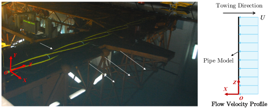
Figure 1: Experimental setup of the flexible pipe VIV test in uniform flow. The uniform flow is generated by passive towing.

The primary physical properties of the test pipe model in the uniform flow case are listed in Table 1.

Table 1: Physical properties of the test pipe model in uniform flow case

Parameter	Value of test model
Pipe model length $L$ (m)	7.90
Outer diameter $D$ (mm)	31.00
Mass in air $\bar{m}$ (kg/m)	1.77
Bending stiffness $EI$ ($\text{\,}\mathrm{N}\mathrm{m}^{2}$)	$1.47\times 10^{3}$
Tensile stiffness $EA$ (N)	$1.45\times 10^{3}$
Damping ratio $\zeta$ (%)	0.3

3.2 Linearly sheared flow cases

The model test was conducted in the ocean basin of the State Key Laboratory of Ocean Engineering at Shanghai Jiao Tong University. The experimental setup, consisting of the rotating rig and the tested pipe model, was installed on the false bottom of the basin, as illustrated in Fig. 2. The flow field was generated by rotating the apparatus via a timing belt driven by a servo motor, and the driven wheel moved at the same given linear velocity via the servo motor during the experiment. This novel VIV experimental apparatus has undergone credibility validation through noise signal analysis, repetitive experiments, and water depth independence tests, as stated in previous studies [34, 35]. Unlike the VIV experiment for bidirectional shear flow discussed later, in this case, a device was positioned at the center of the driven wheel to secure the wheel. The pipe model was tensioned between the edge of the apparatus at the driven wheel and the central fixed device, which was equipped with clamps, U-joints, and a force sensor. The distance from the false bottom to the experimental pipe was $26D$. A pretension force of $550\text{\,}\mathrm{N}$ was applied to the pipe model.

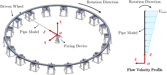
Figure 2: Experimental setup of the flexible pipe VIV test in linearly sheared flow. The linearly sheared flow is generated by the driven wheel rotation. This figure is modified based on the figure in the previous paper [36].

The primary physical properties of the test pipe model in the linearly sheared flow case are listed in Table 2.

Table 2: Physical properties of the test pipe model in linearly sheared flow case

Parameter	Value of test model
Pipe model length $L$ (m)	3.88
Outer diameter $D$ (mm)	28.41
Mass in air $\bar{m}$ (kg/m)	1.24
Bending stiffness $EI$ ($\text{\,}\mathrm{N}\mathrm{m}^{2}$)	$58.6$
Tensile stiffness $EA$ (N)	$9\times 10^{5}$
Damping ratio $\zeta$ (%)	2.58

3.3 Bidirectionally sheared flow cases

The model test was performed in an ocean basin at Shanghai Jiao Tong University. The experimental apparatus was similar to that used in previous linearly sheared flow tests. The test pipe model was installed on two sides through the diameter of the driven gear, and it consisted of clamps, U-joints and a force sensor, as shown in Fig. 3. The force sensor was connected to a tensioner fixed on the driven gear. A pretension force $980\text{\,}\mathrm{N}$ was applied to the pipe model through the tensioner.

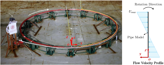
Figure 3: Experimental setup of the flexible pipe VIV test in bidirectionally sheared flow. The bidirectionally sheared flow was generated by the rotation of the driven wheel. This figure is modified from a figure in the previous paper [34].

The primary physical properties of the test pipe model in the bidirectionally sheared flow case are listed in Table 3.

Table 3: Physical properties of the test pipe model in bidirectionally sheared flow case

Parameter	Value of test model
Pipe model length $L$ (m)	7.64
Outer diameter $D$ (mm)	28.41
Mass in air $\bar{m}$ (kg/m)	1.24
Bending stiffness $EI$ ($\text{\,}\mathrm{N}\mathrm{m}^{2}$)	58.6
Tensile stiffness $EA$ (N)	9.4E5
Damping ratio $\zeta$ (%)	2.58

4 Results and discussion

In this manuscript, we introduce the vibration response results and compare three kinds of flow cases; then, a hydrodynamic analysis of two kinds of flow cases, uniform flow and linearly sheared flow, is illustrated. The hydrodynamic analysis of bidirectionally sheared flow cases will be introduced later because of their complexity.

4.1 Uniform flow cases

For uniform flow cases, we introduce two cases: flow velocities $U=$0.40\text{\,}\mathrm{m}\mathrm{/}\mathrm{s}$$ and $1.60\text{\,}\mathrm{m}\mathrm{/}\mathrm{s}$. Fig. 4 represents the distribution of the VIV response in the $U=$0.40\text{\,}\mathrm{m}\mathrm{/}\mathrm{s}$$ case with five subfigures. The subfigure (a) represents the initial displacement of the flexible pipe due to the mean drag force; subfigures (b) and (c) represent the VIV responses in the CF and IL directions, respectively; and subfigures (d) and (e) represent the strain data, respectively. The black line represents the simulation result; the red line represents the experimental result; the blue line represents the VIVANA prediction result; and the red dots represent the strain data measured in the experiment. All the data points are calculated based on the last $20\%$ data, and the VIVANA is a frequency domain model with no time-domain data.

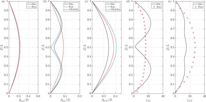
Figure 4: Spanwise distribution of VIV response of uniform flow case at $U=$0.40\text{\,}\mathrm{m}\mathrm{/}\mathrm{s}$$: (a) initial displacement in the IL direction; (b) VIV RMS displacement in the IL direction; (c) VIV RMS displacement in the CF direction; (d) VIV RMS strain in the IL direction; (e) VIV RMS strain in the CF direction. Black line: simulation result; red line and circular symbol: experimental result; blue line: VIVANA result.

VIVANA [37] is applied in this study to compare with the prediction results, as it is also a strip theory based method, and the nodal forces are derived from a forced motion VIV database for a bluff cylinder. As a widely used engineering VIV prediction platform, VIVANA is employed here for the preliminary validation of the CFD numerical results. However, the vortex-induced vibration of a flexible pipe is a highly complex FSI phenomenon, and no prediction software can perfectly replicate the experimental results. Fatigue prediction, which is critical for engineering applications, depends on the displacement, frequency, and traveling wave phenomena. We introduce these results in this section.

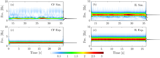
Figure 5: Response frequencies at $Z=0.2L$ of uniform flow $U=$0.40\text{\,}\mathrm{m}\mathrm{/}\mathrm{s}$$ case: (a) time-varying response frequency obtained via a wavelet analysis of the numerical result in the CF direction; (b) time-varying response frequency of the numerical result in the IL direction; (c) time-varying response frequency of the experimental result in the CF direction; (d) time-varying response frequency of the experimental result in the IL direction. Black line on the right represents the general frequency spectrum. White to red: zero to maximum value.

In most flexible pipe VIV experiments, strain signals are measured initially, followed by modal analysis to obtain the VIV displacement. In this study, numerical displacement is converted to strain using the following relationship:

$$\varepsilon_{CF}=\dfrac{\partial^{2}y}{\partial z^{2}}R,$$ (12)

where $R$ represents the radius where the strain gauge is positioned. $\varepsilon_{IL}$ can be obtained via the same method. Experimental strain data are directly obtained during the tests. For the uniform flow case, a bandpass filter is applied during postprocessing, whereas in the linearly sheared and bidirectionally sheared flow cases, unfiltered raw data are used.

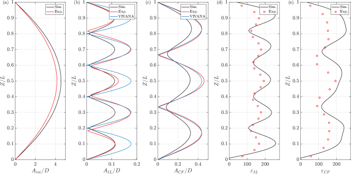
Figure 6: Spanwise distribution of VIV response of uniform flow case at $U=$1.60\text{\,}\mathrm{m}\mathrm{/}\mathrm{s}$$: (a) initial displacement in the IL direction; (b) VIV RMS displacement in the IL direction; (c) VIV RMS displacement in the CF direction; (d) VIV RMS strain in the IL direction; (e) VIV RMS strain in the CF direction. Black line: simulation result; red line and circular symbol: experimental result; blue line: VIVANA prediction result.

However, it should be noted that the modal analysis approach used in this case is still being researched and developed [12, 38, 39]. There are inevitable noise signals during VIV tests, and there is no generalized processing method for flexible-pipe VIV data. Therefore, the experimental strain data also contain a noise signal, but they are still the most reliable benchmark data at present.

Fig. 4 illustrates that the response and strain results of the CFD numerical simulation closely align with the experimental results in terms of the symmetric initial IL displacement. Both the VIVANA model and CFD results predict a second-order response with comparable trends in the IL direction, whereas the experimental results show a first-order dominant response. In the CF direction, all the results indicate a first-order dominant response; however, the CFD model underestimates both the VIV response and the corresponding strain. However, it should be noted that this flow case is a type of low-flow-velocity case for the relatively stiff pipe model, which results in first-order dominance retained in the experimental IL direction, as VIV has just begun to occur at this point in the experiment.

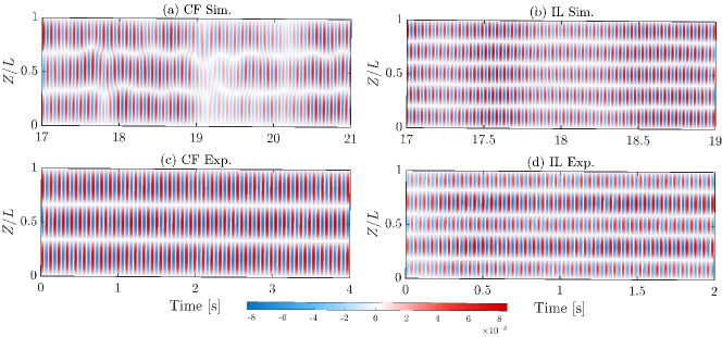
Figure 7: Spatial and temporal distributions of the VIV displacement along the pipe for uniform flow case at $U=$1.60\text{\,}\mathrm{m}\mathrm{/}\mathrm{s}$$: (a) and (b) numerical nondimensional displacement (A/D) in the CF and IL directions, respectively; (c) and (d) experimental nondimensional displacement in the CF and IL directions, respectively. Blue to red: negative amplitude to positive amplitude.

Fig. 5 represents the response frequency at location $Z=0.2L$ in the uniform flow $U=$0.40\text{\,}\mathrm{m}\mathrm{/}\mathrm{s}$$ case. There are two parts in each subfigure: the time-varying response frequency generated by the wavelet transformation on the left and the general amplitude-frequency spectrum on the right. The continuous wavelet transform equation is

$$WT_{f}(a,\tau)=\left\langle f(t),\psi_{a,\tau}(t)\right\rangle=a^{-1/2}\int_{-\infty}^{+\infty}f(t)\psi^{*}\left(\frac{t-\tau}{a}\right)dt,$$ (13)

where $WT_{f}$ is the wavelet transformation coefficient of the time domain signal $f(t)$, which represents the variation in frequency at that time scale. Parameter $a$ is the scale factor, $\tau$ is the shift factor, $\psi(t)$ is the mother wavelet, and the Morlet wavelet is chosen as the mother wavelet. The general amplitude-frequency spectrum is defined as:

$$\mathcal{F}(f)=\sum_{i=1}^{n}\hat{F}_{i}(f),$$ (14)

where $\hat{F}_{i}(f)$ is the PSD at the $i$th data point, and $\mathcal{F}(f)$ is the general amplitude-frequency spectrum obtained by summing the amplitude at the same frequency component for all the data points. This figure shows that the VIV result under these flow conditions exhibits stable first and second order mode responses in the CF and IL directions, respectively, and the numerical simulation in the CF direction presents negligible intermittent responses. The general frequency spectrum clearly has one single dominant peak. The colorbar is omitted in the following text.

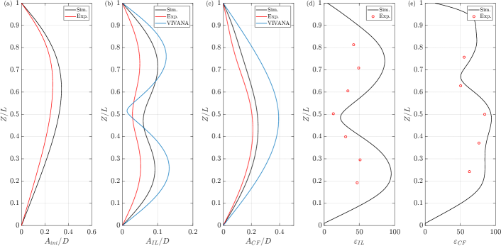
Figure 8: Spanwise distribution of VIV response of linearly sheared flow case at $U_{max}=$0.60\text{\,}\mathrm{m}\mathrm{/}\mathrm{s}$$: (a) initial displacement in the IL direction; (b) VIV RMS displacement in the IL direction; (c) VIV RMS displacement in the CF direction; (d) VIV RMS strain in the IL direction; (e) VIV RMS strain in the CF direction. Black line: simulation result; red line and circular symbols: experimental result; blue line: VIVANA result.

Fig. 6 represents the response of $U=$1.60\text{\,}\mathrm{m}\mathrm{/}\mathrm{s}$$ case, where the initial IL displacement maintains a symmetric distribution with maximum value at $4D$. The experimental and numerical results are in good agreement, with the IL VIV exhibiting a fifth order response and a third order response in the CF direction. The CFD results in the IL direction align more closely with the experimental data than the VIVANA predictions. Additionally, the strain results from the CFD simulation follow the same trend as the experimental data, demonstrating close agreement.

Figure 9: Response frequencies at $Z=0.2L$ of linearly sheared flow case at $U_{max}=$0.60\text{\,}\mathrm{m}\mathrm{/}\mathrm{s}$$ case: (a) time-varying response frequency by wavelet analysis of the numerical result in the CF direction; (b) time-varying response frequency of the numerical result in the IL direction; (c) time-varying response frequency of the experimental result in the CF direction; (d) time-varying response frequency of the experimental result in the IL direction. The black line on the right represents the general frequency spectrum. White to red: zero to maximum value.

Fig. 7 represents the VIV traveling wave phenomenon, and the antinode position variation indicates whether the corresponding VIV response exhibits standing wave or traveling wave characteristics. The results show the vibration response is dominated by the standing wave phenomenon despite a fifth order dominant response in the IL direction. The colorbar is also omitted in the following text.

Figure 10: Spatial and temporal distributions of the VIV displacement along the pipe for the linearly sheared flow case at $U_{max}=$0.60\text{\,}\mathrm{m}\mathrm{/}\mathrm{s}$$: (a) and (b) numerical nondimensional displacement (A/D) in the CF and IL directions, respectively; (c) and (d) experimental nondimensional displacement in the CF and IL directions, respectively. Blue to red: negative amplitude to positive amplitude.

Fig. 11 represents the numerical hydrodynamic response of the uniform flow case $U_{max}=$1.60\text{\,}\mathrm{m}\mathrm{/}\mathrm{s}$$. Hydrodynamic analysis is not the main focus of this manuscript, but readers may find it of interest. The processing methods have also been uploaded to GitHub, while a more detailed analysis will be published in future work.

The hydrodynamic distribution of a flexible pipe undergoing VIV can be expressed as:

$$EI\frac{\partial^{4}y(z,t)}{\partial z^{4}}-\frac{\partial}{\partial z}{\left[T\frac{\partial y(z,t)}{\partial z}\right]}+c\frac{\partial y(z,t)}{\partial t}+\bar{m}\frac{\partial^{2}y(z,t)}{\partial t^{2}}=f_{CF}(z,t),$$ (15)

and the force can be decomposed as excitation and added mass forces:

$$f_{CF}(t) =\underbrace{\frac{1}{2\sqrt{2}\dot{y}_{rms}}\rho DV^{2}C_{e}(t)\dot{y}(t)}_{F_{e}}\underbrace{-\vphantom{\frac{1}{2\sqrt{2}\dot{y}_{rms}}}\frac{\pi D^{2}}{4}\rho C_{m}(t)\ddot{y}(t)}_{F_{m}},$$ (16)

then the nonlinear regression method is applied for two coefficients distribution in Fig. 11. The phase difference $\phi_{xy}$ is the phase difference of IL and CF responses as:

$$\phi_{xy}(z,t)=\left[\phi_{x}(z,t)-\frac{f_{x}(z,t)}{f_{y}(z,t)}\phi_{y}(z,t),\quad\bmod 360^{\circ}\right],$$ (17)

The hydrodynamic coefficients, phase, and vortex patterns are interconnected. The method proposed in this paper enables the study of engineering FSI vortex-induced vibration to become a feasible research topic, which will be introduced in further study.

Figure 11: VIV response along the pipe of the uniform flow case $U=$1.60\text{\,}\mathrm{m}\mathrm{/}\mathrm{s}$$ of simulation results. (a) spanwise distribution of VIV response of initial displacement (blue line), IL (orange line) and CF (black line) RMS displacement; (b) histogram of phase difference; (c) excitation (black) and added mass (red) coefficients distribution; (d) to (h) instantaneous vorticity contours $\omega_{z}$ correspond to the red symbols in subfigure (a).

4.2 Linearly sheared flow cases

For linearly sheared flow cases, we will introduce two velocity cases as $U_{max}=$0.60\text{\,}\mathrm{m}\mathrm{/}\mathrm{s}$$ and $1.00\text{\,}\mathrm{m}\mathrm{/}\mathrm{s}$. Fig. 8 represents the VIV response in the linearly sheared flow case at $U_{max}=$0.60\text{\,}\mathrm{m}\mathrm{/}\mathrm{s}$$, and the initial IL displacement exhibits an asymmetric distribution. Due to the sheared flow velocity profile, regions with higher flow velocities have larger initial displacements. The IL and CF VIV responses are dominated by the second order and first order, respectively. The numerical simulation results align more closely with the experimental data than those from VIVANA.

Figure 12: Spanwise distribution of the VIV response of linearly sheared flow case at $U_{max}=$1.00\text{\,}\mathrm{m}\mathrm{/}\mathrm{s}$$: (a) initial displacement in the IL direction; (b) VIV RMS displacement in the IL direction; (c) VIV RMS displacement in the CF direction; (d) VIV RMS strain in the IL direction; (e) VIV RMS strain in the CF direction. Black line: simulation result; red line and circular symbol: experimental result; blue line: VIVANA result.

Unlike the uniform flow experiment, which includes 25 strain measurement points in the CF direction and 19 in the IL direction, the linearly sheared flow experiment involves 7 CF strain measurement points and 5 in the IL direction. Owing to the fragility of FBG sensors, in this VIV experiment, the overall displacement is reconstructed via a reduced number of measurement points. In practice, the requirements for experimental modal analysis can be met as long as the number of measurement points exceeds the highest dominant vibration mode [40]. The numerical strain results match well with the experimental results.

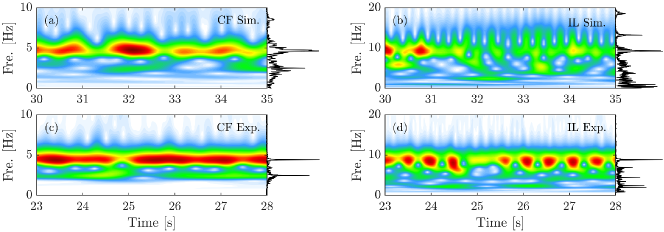
Figure 13: Response frequencies at $Z=0.2L$ in the linearly sheared flow case at $U_{max}=$1.00\text{\,}\mathrm{m}\mathrm{/}\mathrm{s}$$ case: (a) time-varying response frequency via wavelet analysis of the numerical result in the CF direction; (b) time-varying response frequency of the numerical result in the IL direction; (c) time-varying response frequency of the experimental result in the CF direction; (d) time-varying response frequency of the experimental result in the IL direction. Black line on the right represents the general frequency spectrum. White to red: zero to maximum value.

Unlike the VIVANA prediction results, the IL and CF responses contain multiple first-order components. As Fig. 9 shows, the VIV experiments generally exhibit a time-sharing phenomenon, where the dominant frequency in the wavelet result remains singular over time [41]. This is one basic assumption in current engineering prediction models such as VIVANA. However, experimental data often contain additional harmonic components that do not dominate the vibration but result in differences in the prediction results, as shown in subfigures (b) and (d).

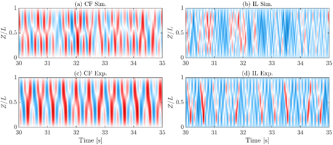
Figure 14: Spatial and temporal distributions of the VIV displacement along the pipe for the linearly sheared flow case at $U_{max}=$1.00\text{\,}\mathrm{m}\mathrm{/}\mathrm{s}$$: (a) and (b) numerical nondimensional displacement (A/D) in the CF and IL directions, respectively; (c) and (d) experimental nondimensional displacement in the CF and IL directions, respectively. Blue to red: negative amplitude to positive amplitude.

Fig. 12 represents the response result of linearly sheared flow case $U_{max}=$1.00\text{\,}\mathrm{m}\mathrm{/}\mathrm{s}$$. Similar to the previous case, the initial IL displacement exhibits an asymmetric distribution with the third order dominant response in the IL direction and second order dominant response in the CF direction. Meanwhile, in this flow case, both the VIVANA predictions and the numerical simulations in this study show good agreement with the experimental results. Moreover, the strain results from the numerical simulation closely match the experimental data in both trend and magnitude. The numerical simulation results are higher than the experimental results.

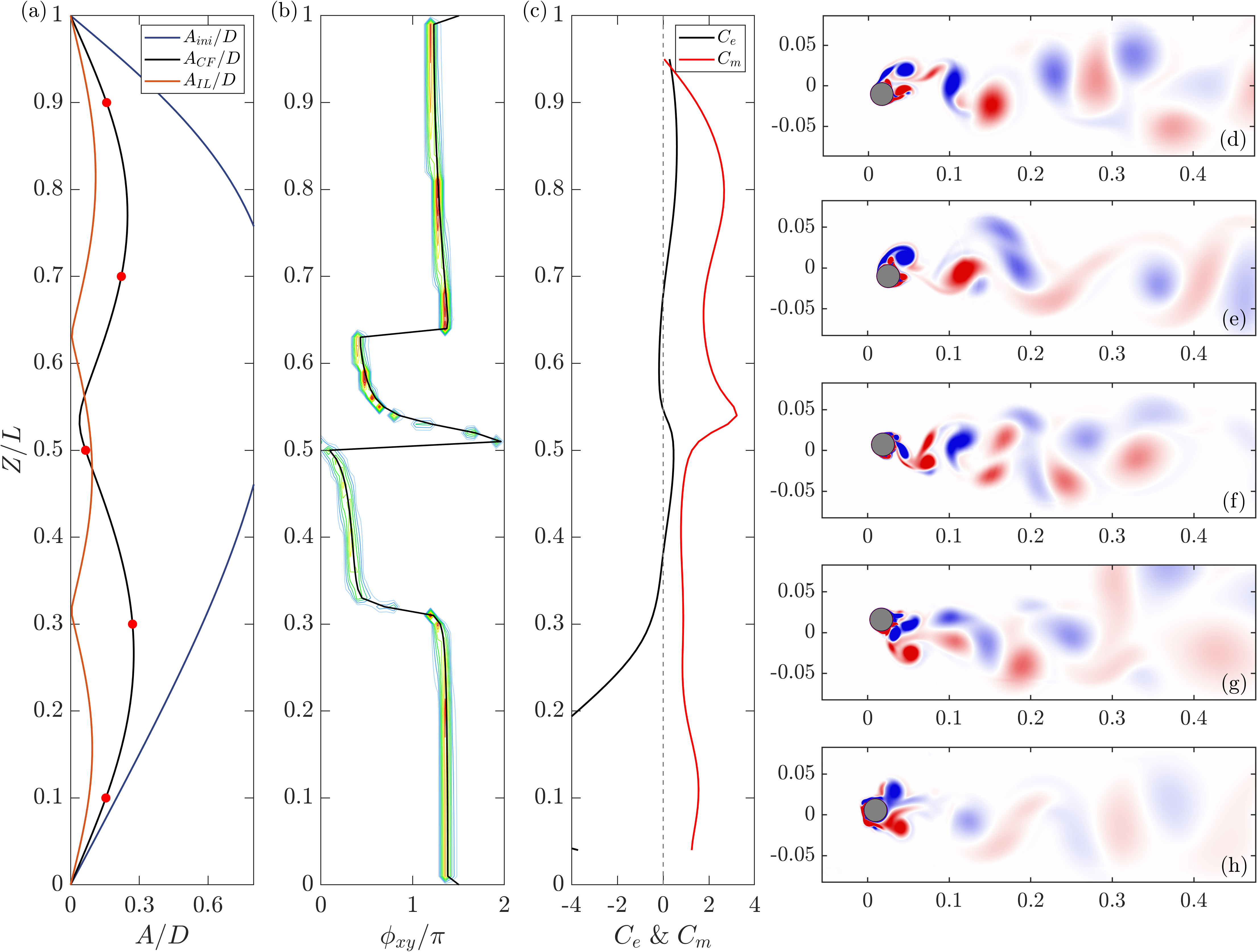
Figure 15: VIV response along the pipe of the linearly sheared flow case $U_{max}=$1.00\text{\,}\mathrm{m}\mathrm{/}\mathrm{s}$$ of simulation results. (a) spanwise distribution of VIV response of initial displacement (blue line), IL (orange line) and CF (black line) RMS displacement; (b) histogram of phase difference; (c) excitation (black) and added mass (red) coefficients distribution; (d) to (h) instantaneous vorticity contours $\omega_{z}$ correspond to the red symbols in subfigure (a).

Fig. 12 represents the response result in the linearly sheared flow case $U_{max}=$1.00\text{\,}\mathrm{m}\mathrm{/}\mathrm{s}$$. Similar to the previous case, in this case, the initial IL displacement has an asymmetric distribution, with a third-order dominant response in the IL direction and a second-order dominant response in the CF direction. Moreover, in this flow case, both the VIVANA predictions and the numerical simulations show good agreement with the experimental results. Moreover, the strain results from the numerical simulation closely match the experimental data in both trend and magnitude. The numerical simulation results are better than the experimental results.

Fig. 15 represents the hydrodynamic result of linearly sheared flow case of $U_{max}=$1.00\text{\,}\mathrm{m}\mathrm{/}\mathrm{s}$$. It can be seen that the phase difference discontinuity is related to the zero point in the IL direction, and the added mass coefficients are positive through the test pipe.

4.3 Bidirectionally sheared flow cases

In this flow case, we introduce three flow velocity cases: $U_{max}=$0.48\text{\,}\mathrm{m}\mathrm{/}\mathrm{s}$$, $0.77\text{\,}\mathrm{m}\mathrm{/}\mathrm{s}$ and $0.99\text{\,}\mathrm{m}\mathrm{/}\mathrm{s}$.

The two flow conditions discussed above have been widely studied in academia and engineering fields, with established engineering prediction frameworks available, reinforcing the credibility of the numerical simulation results presented in this study. However, bidirectionally sheared flow was first experimentally investigated in a laboratory in 2022, revealing several phenomena that deviate from the prevailing understanding of vortex-induced vibration. Given the large experimental scale and the impracticality of directly observing the flow field, the numerical simulation scheme developed in this study could serve as a tool for future fluid mechanism investigations. Nevertheless, owing to length constraints, this paper focuses primarily on a comparative study of the VIV response under the discussed flow conditions.

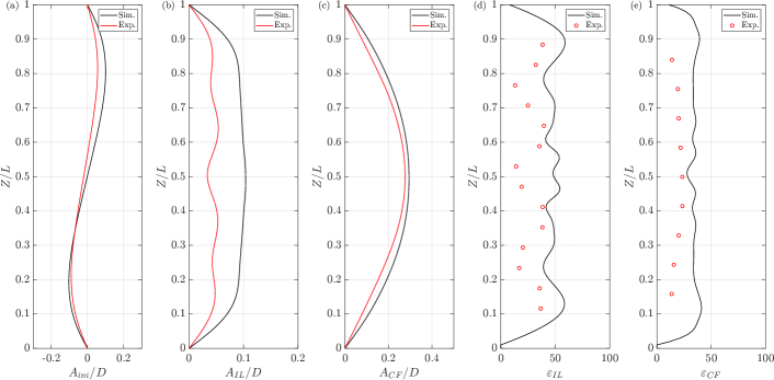
Figure 16: Spanwise distribution of VIV response in the bidirectionally sheared flow case at $U_{max}=$0.48\text{\,}\mathrm{m}\mathrm{/}\mathrm{s}$$: (a) initial displacement in the IL direction; (b) VIV RMS displacement in the IL direction; (c) VIV RMS displacement in the CF direction; (d) VIV RMS strain in the IL direction; (e) VIV RMS strain in the CF direction. Black line: simulation result; red line and circular symbol: experimental result.

Fig. 16 represents the VIV response in the bidirectionally sheared flow case at $U_{max}=$0.48\text{\,}\mathrm{m}\mathrm{/}\mathrm{s}$$. There is currently no existing engineering VIV prediction framework for this flow field VIV now. The initial IL displacement displays an antisymmetric distribution with a second-order modal shape. We need to analyze the IL and CF direction responses by combining the results of time-frequency analyses as Fig. 17 shows.

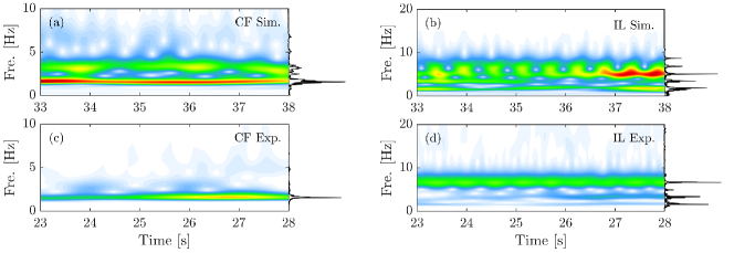
Figure 17: Response frequencies at $Z=0.2L$ of bidirectionally sheared flow case at $U_{max}=$0.48\text{\,}\mathrm{m}\mathrm{/}\mathrm{s}$$: (a) time-varying response frequency obtained via wavelet analysis of the numerical result in the CF direction; (b) time-varying response frequency of the numerical result in the IL direction; (c) time-varying response frequency of the experimental result in the CF direction; (d) time-varying response frequency of the experimental result in the IL direction. Black line on the right represents the general frequency spectrum. White to red: zero to maximum value.

Notably, this flow velocity is relatively low, with a first order dominant CF response at nearly $0.3D$, but a fairly complex response is observed in the IL direction. In the general frequency spectrum, a first to fifthorder response can be observed, whereas a fourth order response is shown in the experimental result and a third-order response is present in the simulation result.

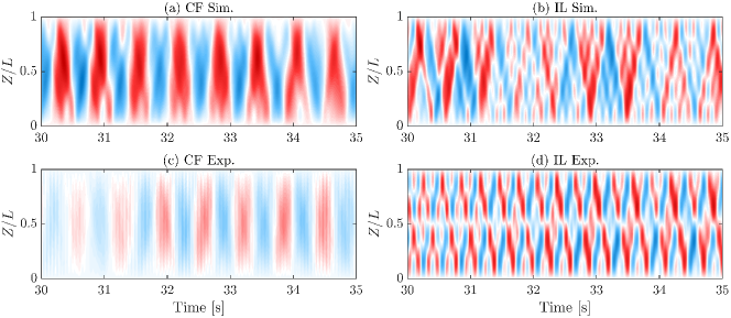
Figure 18: Spatial and temporal distributions of the VIV displacement along the pipe of bidirectionally sheared flow case at $U_{max}=$0.48\text{\,}\mathrm{m}\mathrm{/}\mathrm{s}$$: (a) and (b) numerical nondimensional displacement (A/D) in the CF and IL directions, respectively; (c) and (d) experimental nondimensional displacement in the CF and IL directions, respectively. Blue to red: negative amplitude to positive amplitude.

The common feature is that under such a low flow velocity condition, there is a distinct multifrequency response, but the dominant mode is different. Notably, in the numerical simulation method used in this study, constant tension is assumed during VIV. However, in the actual experiment, the tensioners at the end of the system apply variable tension through springs. Structural nonlinearity was not incorporated in the present numerical simulation. In our previous VIV engineering prediction studies [42], where variable tension was considered, we found that the experimental riser, which is composed of multiple layers, exhibits a variable axial stiffness ($EA$) under vortex-induced vibration, which does not always align with the material test value. We are currently developing a more accurate model to account for the effects of variable tension in future studies. Moreover, the traveling wave response also has a significant effect on this multi-frequency response. We confirm that the multifrequency IL phenomenon under these flow velocity conditions is real rather than an experimental error.

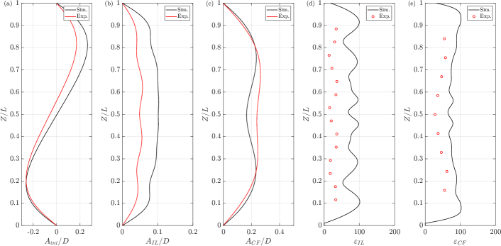
Figure 19: Spanwise distribution of VIV response of bidirectionally sheared flow case at $U_{max}=$0.77\text{\,}\mathrm{m}\mathrm{/}\mathrm{s}$$: (a) initial displacement in the IL direction; (b) VIV RMS displacement in the IL direction; (c) VIV RMS displacement in the CF direction; (d) VIV RMS strain in the IL direction; (e) VIV RMS strain in the CF direction. Black line: simulation result; red line and circular symbols: experimental result.

Fig. 18 represents the spatial and temporal distributions of the VIV response. There exists an obvious traveling phenomenon in the IL direction with high order response, whereas the CF response is first order dominated.

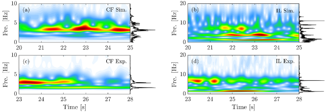
Figure 20: Response frequencies at $Z=0.2L$ of bidirectionally sheared flow case at $U_{max}=$0.77\text{\,}\mathrm{m}\mathrm{/}\mathrm{s}$$: (a) time-varying response frequency by wavelet analysis of numerical result in the CF direction; (b) time-varying response frequency of numerical result in the IL direction; (c) time-varying response frequency of experimental result in the CF direction; (d) time-varying response frequency of experimental result in the IL direction. Black line on the right represents the general frequency spectrum. White to red: zero to maximum value.

Fig. 19 and Fig. 20 represent the VIV response of the bidirectionally sheared case of $U_{max}=$0.77\text{\,}\mathrm{m}\mathrm{/}\mathrm{s}$$. In this flow case, the VIV response in the CF direction represents multi-frequency of the first order and the second order, the numerical result and experimental result are close. A complex multi-frequency response is also observed in the IL direction. Compared with the experimental results, the numerical simulation results in this study consistently yield higher strain values.

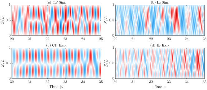
Figure 21: Spatial and temporal distributions of the VIV displacement along the pipe of bidirectionally sheared flow case at $U_{max}=$0.77\text{\,}\mathrm{m}\mathrm{/}\mathrm{s}$$: (a) and (b) numerical nondimensional displacement (A/D) in the CF and IL directions, respectively; (c) and (d) experimental nondimensional displacement in the CF and IL directions, respectively. Blue to red: negative amplitude to positive amplitude.

Fig. 21 represents the obvious traveling phenomenon in both the CF and the IL directions, with a low second-order response in the CF direction, which is a typical phenomenon observed experimentally. Fig. 22 to Fig. 24 illustrate the VIV response results in the bidirectionally sheared flow case at $U_{max}=$0.99\text{\,}\mathrm{m}\mathrm{/}\mathrm{s}$$. Similarly, an antisymmeric initial IL response exists, with the VIV response in the CF direction displaying second-order dominance and that in the IL direction exhibiting considerable complexity.

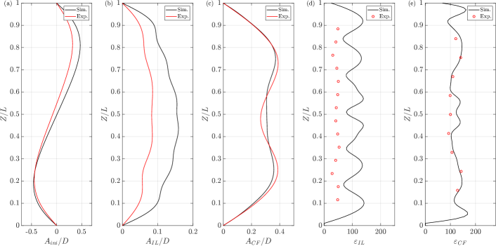
Figure 22: Spanwise distribution of VIV response of bidirectionally sheared flow case at $U_{max}=$0.99\text{\,}\mathrm{m}\mathrm{/}\mathrm{s}$$: (a) initial displacement in the IL direction; (b) VIV RMS displacement in the IL direction; (c) VIV RMS displacement in the CF direction; (d) VIV RMS strain in the IL direction; (e) VIV RMS strain in the CF direction. Black line: simulation result; red line and circular symbols: experimental result.

The numerical simulation results in the CF direction are in good agreement with the experimental results in terms of both response and strain. However, the numerical simulation results in the IL direction are higher than the experimental results. The initial IL displacement in the numerical simulation is more symmetric than that in the experimental results. This discrepancy likely arises from the difficulty in maintaining a consistently perfect antisymmetric field around the pipe model during the experiment.

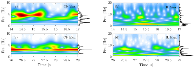
Figure 23: Response frequencies at $Z=0.2L$ of bidirectionally sheared flow case at $U_{max}=$0.99\text{\,}\mathrm{m}\mathrm{/}\mathrm{s}$$: (a) time-varying response frequency by wavelet analysis of the numerical result in the CF direction; (b) time-varying response frequency of the numerical result in the IL direction; (c) time-varying response frequency of the experimental result in the CF direction; (d) time-varying response frequency of the experimental result in the IL direction. Black line on the right represents the general frequency spectrum. White to red: zero to maximum value.

Fig. 22 to Fig. 24 represent the VIV response in the bidirectionally sheared flow case at $U_{max}=$0.99\text{\,}\mathrm{m}\mathrm{/}\mathrm{s}$$. The initial IL displacement maintains an antisymmetric distribution, exhibiting a clear multifrequency response in the IL direction. Moreover, a second-order response is primarily dominant in the CF direction, with third-order contributions. In the bidirectionally sheared flow simulation, the numerical results in the IL direction consistently exceed the experimental values, whereas the results in the CF direction closely align with the experimental data. The strain results follow a similar pattern. During the experiment, the IL VIV response always contains an obvious first-order response with a high-order component, which is also found in the simulation results. The numerical simulations in this study capture this phenomenon, and more detailed hydrodynamic investigations will be conducted in the future.

A distinct multifrequency response under these flow velocity conditions is also observed in the CF direction, as Fig. 23 (a) and (c) show, with a distinct traveling wave response in both the CF and the IL directions.

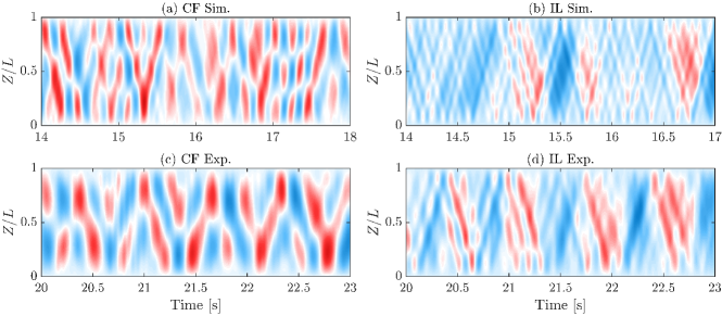
Figure 24: Spatial and temporal distributions of the VIV displacement along the pipe of bidirectionally sheared flow case at $U_{max}=$0.99\text{\,}\mathrm{m}\mathrm{/}\mathrm{s}$$: (a) and (b) numerical nondimensional displacement (A/D) in the CF and IL directions, respectively; (c) and (d) experimental nondimensional displacement in the CF and IL directions, respectively. Blue to red: negative amplitude to positive amplitude.

5 Summary

In this study, a validated numerical framework for predicting the VIV of a flexible pipe in steady flows is introduced, integrating URANS-based fluid dynamics with a structural finite element model through a weak coupling scheme. The framework is systematically validated on the basis of three benchmark experimental cases: uniform, linearly sheared, and bidirectionally sheared flows. The VIV responses in terms of the amplitude, frequency, and strain results are compared. The results show that the proposed model is able to capture certain unique phenomena observed in experiments, with higher accuracy than VIVANA in some conditions. This model will be used to analyze the mechanisms of fluid-structure interaction later.

However, the model has the following limitations: 1) The Euler-Bernoulli beam theory is applied for the structural model, which may not be sufficient for the more nonlinear beam models required for structures such as steel catenary risers. 2) The model does not account for the time-domain variation in tension, which introduces some errors in the simulation of high-order responses. 3) For multipipe systems, it remains unclear whether URANS can accurately capture the wake field and the potential problem with reverse energy cascades for LES strips. The applicability of the strip method to multipipe systems will be studied further in the future.

Overall, we disclose all the published experimental and numerical results, with the hope of supporting CFD numerical simulation research on vortex-induced vibration to accelerate the application of new technologies.

Data availability

The corresponding benchmark experimental data and VIV simulation code can be found in the GitHub repository: https://github.com/xuepengfu/VIVdatashare. There are also additional case results in this repository.

The program and experimental data will be made publicly available as the research progresses.

Appendix A Finite element model of a tensioned flexible pipe

The two degrees of freedom beam model (IL and CF directions) are applied in the present study. The element mass matrix is given by:

$$\boldsymbol{M}^{e}=\frac{\bar{m}l}{420}\left[\begin{array}[]{cccc}156&22l&54&-13l\\ 22l&4l^{2}&13l&-3l^{2}\\ 54&13l&156&-22l\\ -13l&-3l^{2}&-22l&4l^{2}\end{array}\right],$$ (18)

and the stiffness matrix is:

$$\boldsymbol{K}^{e}=\boldsymbol{K}^{E}+\boldsymbol{K}^{T},$$ (19)

$$\boldsymbol{K}^{E}=\frac{EI}{l^{3}}\left[\begin{array}[]{cccc}12&6l&-12&6l\\ 6l&4l^{2}&-6l&2l^{2}\\ -12&-6l&12&-6l\\ 6l&2l^{2}&-6l&4l^{2}\end{array}\right],$$

$$\boldsymbol{K}^{T}=\frac{T}{30l}\left[\begin{array}[]{cccc}36&3l&-36&3l\\ 3l&4l^{2}&-3l&-l^{2}\\ -36&-3l&36&-3l\\ 3l&-l^{2}&-3l&4l^{2}\end{array}\right],$$

where Rayleigh damping is used for the damping matrix, expressed as:

$$\boldsymbol{C}=\alpha\boldsymbol{M}+\beta\boldsymbol{K},$$ (20)

$$\alpha=\frac{2(\zeta_{1}\omega_{2}-\zeta_{2}\omega_{1})}{(\omega_{1}+\omega_{2})(\omega_{2}-\omega_{1})}\omega_{1}\omega_{2},$$

$$\beta=\frac{2(\zeta_{1}\omega_{2}-\zeta_{2}\omega_{1})}{(\omega_{1}+\omega_{2})(\omega_{2}-\omega_{1})},$$

where $\bar{m}$ is the unit mass, $l$ is the length of the riser, $EI$ is the bending stiffness, $T$ is the tension, $\omega_{1}$ and $\omega_{2}$ are the first two natural circular frequencies of the pipe, and $\zeta_{1}$ and $\zeta_{2}$ are the first two damping ratios.

The system mass and stiffness matrices are obtained by assembling the element mass and stiffness matrices as:

$$\boldsymbol{K}=\left[\begin{array}[]{cccccc}\boldsymbol{K}^{e}_{(1.1)}&\cdots&0&\cdots&0\\ &\ddots&\vdots&\ddots&\vdots\\ &&\boldsymbol{K}^{e}_{(i.2)}+\boldsymbol{K}^{e}_{((i+1).1)}&\cdots&0\\ &\text{symmetric}&&\ddots&\vdots\\ &&&&\boldsymbol{K}^{e}_{(N.2)}\end{array}\right]$$ (21)

$$\boldsymbol{M}=\left[\begin{array}[]{cccccc}\boldsymbol{M}^{e}_{(1.1)}&\cdots&0&\cdots&0\\ &\ddots&\vdots&\ddots&\vdots\\ &&\boldsymbol{M}^{e}_{(i.2)}+\boldsymbol{M}^{e}_{((i+1).1)}&\cdots&0\\ &\text{symmetric}&&\ddots&\vdots\\ &&&&\boldsymbol{M}^{e}_{(N.2)}\end{array}\right]$$ (22)

Appendix B Independence test

Fig. 25 show three different mesh number cases in uniform flow as examples. The cell numbers for mesh 1, mesh 2 and mesh 3 are 1418240, 1063040 and 909440, respectively. The results show that there is no difference among these cases, and mesh 2, as the median case, is chosen. We refer to the results of our previous numerical simulation studies to determine the appropriate mesh quality [29, 30].

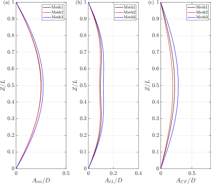
Figure 25: Independence test of the number of meshes used in the flow case of $U=$0.40\text{\,}\mathrm{m}\mathrm{/}\mathrm{s}$$: (a) initial IL displacement; (b) IL response; (c) CF response.

With respect to the number of strips, ensuring the distribution of three strips between nodes in the highest excitation mode can provide accurate prediction results [24]. However, this approach has not been validated in the bidirectionally sheared flow case. LABEL:bistripn shows a comparison of different strip methods in the bidirectionally sheared flow case with $U_{max}=$1.15\text{\,}\mathrm{m}\mathrm{/}\mathrm{s}$$. The results show that there are no obvious differences among these strip setups. Notably, 20 strips are applied in the present study.

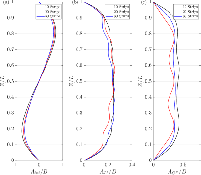
Figure 26: Independence tests with 10 (black line), 20 (red line), and 30 (blue line) strips in the bidirectionally sheared flow case with $U_{max}=$1.15\text{\,}\mathrm{m}\mathrm{/}\mathrm{s}$$: (a) initial IL displacement; (b) IL response; (c) CF response.

Appendix C Comparison of weak coupling and strong coupling results

The strong coupling algorithm is implemented for individual time steps to meet a high convergence standard, the FSI strong coupling algorithm withthe Aitkenn relaxation method [43] is shown in 2.

Input: Solid field parameters; Flow field parameters.

Output: Structural response $\boldsymbol{\xi}_{s}$ and flow velocity and pressure field $\boldsymbol{u}_{f},p_{f}$.

1 $t\leftarrow 0$

2 $j_{in}\leftarrow 10,\;\epsilon_{in}\leftarrow 1\times 10^{-6}$

3while $t<t_{end}$ do

4    $j\leftarrow 0,\;\gamma_{j}\leftarrow 0.5,\;\omega_{j}\leftarrow 1-\gamma_{j}$

5   while $j<j_{in}\;||\;\epsilon>\epsilon_{in}$ do

6       $\boldsymbol{F}_{f,j}^{t}$ $\leftarrow$ solve $\mathcal{N}(\boldsymbol{u}_{f},p_{f})=0$

7      $\boldsymbol{\xi}_{s,j}^{t}$ $\leftarrow$ solve $\mathcal{S}(\boldsymbol{u}_{s})-\boldsymbol{F}_{f}=0$

8      Update mesh with $\boldsymbol{\xi}_{s,j}^{t}$ at $t$

9      $\Delta\boldsymbol{\xi}_{j}\leftarrow\boldsymbol{\xi}_{s,j-1}-\boldsymbol{\xi}_{s,j}$

10      $\epsilon\leftarrow|\Delta\boldsymbol{\xi}_{j}|$

11      $\Delta\boldsymbol{\xi}_{j-1}\leftarrow\boldsymbol{\xi}_{s,j-2}-\boldsymbol{\xi}_{s,j-1}$

12      $\gamma_{j}=\gamma_{j-1}+(\gamma_{j-1}-1)(\Delta\boldsymbol{\xi}_{j-1}-\Delta\boldsymbol{\xi}_{j})\Delta\boldsymbol{\xi}_{j}/(\Delta\boldsymbol{\xi}_{j-1}-\Delta\boldsymbol{\xi}_{j})^{2}$

13      $\omega_{j}=1-\gamma_{j}$

14      $\boldsymbol{\xi}_{s,j}^{t}\leftarrow\omega_{j}\boldsymbol{\xi}_{s,j}^{t}+(1-\omega_{j})\boldsymbol{\xi}_{s,j-1}^{t}$

15      $j\leftarrow j+1$

16    end while

17   $t\leftarrow t+\Delta t$

18 end while

Algorithm 2 Strong coupling algorithm of FSI simulation with Aitken relaxation.

Fig. 27 shows a comparison of the results of the weak and strong coupling algorithms. There is no significant difference between the two sets of results. However, three times as many simulations are required in the strong coupling case. Causin et al. [44] analyzed the stability of FSI governing equations for flat-plate flows, yielding a characteristic equation $\chi(s)$ with:

$$\chi(-\infty)=-\infty,\quad\chi(-1)=a+\frac{4}{\Delta t^{2}}(\rho_{f}\mu_{i}-\rho_{s}h_{s}),$$ (23)

where $a$ is a function of the material Young’s modulus $f(E)$, $\rho_{f}$ and $\rho_{s}$ are the fluid and solid densities, $\mu_{i}$ is the eigenvalue of the added mass operator $\mathcal{M}_{A}$, and $h_{s}$ is the structural characteristic length. If $\chi(-1)>0$, the equation becomes unconditionally unstable. Thus, instability may occur when $\rho_{s}/\rho_{f}<1$ or with high Young’s modulus values.

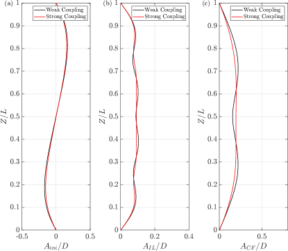
Figure 27: Comparison results of weak coupling and strong coupling algorithm.

For VIV problems, flexible risers typically have mass ratios above $3.00$, and rigid cylinders have mass ratios above 1.00; therefore, the weak coupling algorithm is applicable for solving VIV problems. For practical flexible ocean engineering structures, in engineering software such as RIFLEX [45], weak coupling is adopted for structural time-domain response simulations, which is considered to achieve sufficient engineering prediction accuracy. However, a submerged floating tunnel, a newly emerging circular structure in ocean engineering with a structural density similar to that of water, may require a strong coupling algorithm to perform accurate numerical simulations. This issue will be investigated in the future.

References

- Huera-Huarte [2024] F. Huera-Huarte, Vortex-induced vibration of flexible cylinders in cross-flow, Annual Review of Fluid Mechanics 57 (2024).
- Govardhan and Williamson [2000] R. Govardhan, C. Williamson, Modes of vortex formation and frequency response of a freely vibrating cylinder, Journal of Fluid Mechanics 420 (2000) 85–130.
- Dahl et al. [2006] J. Dahl, F. Hover, M. Triantafyllou, Two-degree-of-freedom vortex-induced vibrations using a force assisted apparatus, Journal of Fluids and Structures 22 (2006) 807–18.
- Qu and Metrikine [2020] Y. Qu, A. V. Metrikine, A single van der pol wake oscillator model for coupled cross-flow and in-line vortex-induced vibrations, Ocean Engineering 196 (2020) 106732.
- Soares and Srinil [2021] B. Soares, N. Srinil, Modelling of wake-induced vibrations of tandem cylinders with a nonlinear wake-deficit oscillator, Journal of Fluids and Structures 105 (2021) 103340.
- Qu et al. [2025] Y. Qu, W. Xu, S. Fu, Y. Song, Vortex-induced vibrations of an elastically supported rigid cylinder in a dual-mass system, Journal of Sound and Vibration (2025) 118940.
- Vandiver and Ma [2017] J. K. Vandiver, L. Ma, Does more tension reduce viv?, in: International Conference on Offshore Mechanics and Arctic Engineering, volume 57700, American Society of Mechanical Engineers, 2017, p. V05BT04A039.
- Lu et al. [2018] Z. Lu, S. Fu, M. Zhang, H. Ren, L. Song, A modal space based direct method for vortex-induced vibration prediction of flexible risers, Ocean Engineering 152 (2018) 191–202.
- Thorsen et al. [2016] M. J. Thorsen, S. Sævik, C. M. Larsen, Time domain simulation of vortex-induced vibrations in stationary and oscillating flows, Journal of Fluids and Structures 61 (2016) 1–19.
- Trim et al. [2005] A. Trim, H. Braaten, H. Lie, M. Tognarelli, Experimental investigation of vortex-induced vibration of long marine risers, Journal of fluids and structures 21 (2005) 335–61.
- Tognarelli et al. [2004] M. Tognarelli, S. Slocum, W. Frank, R. Campbell, Viv response of a long flexible cylinder in uniform and linearly sheared currents, in: Offshore technology conference, OTC, 2004, pp. OTC–16338.
- Chaplin et al. [2005] J. Chaplin, P. Bearman, F. H. Huarte, R. Pattenden, Laboratory measurements of vortex-induced vibrations of a vertical tension riser in a stepped current, Journal of fluids and structures 21 (2005) 3–24.
- Vandiver et al. [2005] J. Vandiver, H. Marcollo, S. Swithenbank, V. Jhingran, High mode number vortex-induced vibration field experiments, in: Offshore technology conference, OTC, 2005, pp. OTC–17383.
- Resvanis et al. [2023] T. L. Resvanis, J. K. Vandiver, S. McNeill, A report from the drilling riser viv and wellhead fatigue jip: Full-scale drilling riser viv measurements and comparisons with predictions, in: International Conference on Offshore Mechanics and Arctic Engineering, volume 86892, American Society of Mechanical Engineers, 2023, p. V007T08A031.
- Song et al. [2016] L. Song, S. Fu, J. Cao, L. Ma, J. Wu, An investigation into the hydrodynamics of a flexible riser undergoing vortex-induced vibration, Journal of Fluids and Structures 63 (2016) 325–50.
- Wu et al. [2010] J. Wu, C. M. Larsen, H. Lie, Estimation of hydrodynamic coefficients for viv of slender beam at high mode orders, in: International Conference on Offshore Mechanics and Arctic Engineering, volume 49149, 2010, pp. 557–66.
- Baek and Karniadakis [2012] H. Baek, G. E. Karniadakis, A convergence study of a new partitioned fluid-structure interaction algorithm based on fictitious mass and damping, Journal of Computational Physics 231 (2012) 629–52.
- Bourguet et al. [2011] R. Bourguet, G. E. Karniadakis, M. S. Triantafyllou, Vortex-induced vibrations of a long flexible cylinder in shear flow, Journal of fluid mechanics 677 (2011) 342–82.
- Fan et al. [2019] D. Fan, Z. Wang, M. S. Triantafyllou, G. E. Karniadakis, Mapping the properties of the vortex-induced vibrations of flexible cylinders in uniform oncoming flow, Journal of Fluid Mechanics 881 (2019) 815–58.
- Wang et al. [2021] Z. Wang, D. Fan, M. S. Triantafyllou, G. E. Karniadakis, A large-eddy simulation study on the similarity between free vibrations of a flexible cylinder and forced vibrations of a rigid cylinder, Journal of Fluids and Structures 101 (2021) 103223.
- Herfjord et al. [1999] K. Herfjord, S. O. Drange, T. Kvamsdal, Assessment of vortex-induced vibrations on deepwater risers by considering fluid-structure interaction, Journal of Offshore Mechanics and Arctic Engineering 121 (1999) 207–12.
- Willden and Graham [2004] R. H. Willden, J. M. R. Graham, Multi-modal vortex-induced vibrations of a vertical riser pipe subject to a uniform current profile, European Journal of Mechanics-B/Fluids 23 (2004) 209–18.
- Bao et al. [2016] Y. Bao, R. Palacios, M. Graham, S. Sherwin, Generalized thick strip modelling for vortex-induced vibration of long flexible cylinders, Journal of Computational Physics 321 (2016) 1079–97.
- Chaplin et al. [2005] J. Chaplin, P. W. Bearman, Y. Cheng, E. Fontaine, J. Graham, K. Herfjord, F. H. Huarte, M. Isherwood, K. Lambrakos, C. Larsen, et al., Blind predictions of laboratory measurements of vortex-induced vibrations of a tension riser, Journal of fluids and structures 21 (2005) 25–40.
- Deng et al. [2021] D. Deng, W. Zhao, D. Wan, Numerical study of vortex-induced vibration of a flexible cylinder with large aspect ratios in oscillatory flows, Ocean Engineering 238 (2021) 109730.
- Pope [2000] S. B. Pope, Turbulent Flows, Cambridge University Press, 2000.
- Menter et al. [2003] F. R. Menter, M. Kuntz, R. Langtry, et al., Ten years of industrial experience with the sst turbulence model, Turbulence, heat and mass transfer 4 (2003) 625–32.
- Jasak et al. [2007] H. Jasak, A. Jemcov, Z. Tukovic, et al., Openfoam: A c++ library for complex physics simulations, in: International workshop on coupled methods in numerical dynamics, volume 1000, Dubrovnik, Croatia), 2007, pp. 1–20.
- Fu et al. [2022] X. Fu, S. Fu, M. Zhang, Z. Han, H. Ren, Y. Xu, B. Zhao, Frequency capture phenomenon in tandem cylinders with different diameters undergoing flow-induced vibration, Physics of Fluids 34 (2022).
- Fu et al. [2023] X. Fu, S. Fu, Z. Han, Z. Niu, M. Zhang, B. Zhao, Numerical simulations of 2-dof vortex-induced vibration of a circular cylinder in two and three dimensions: A comparison study, Journal of Ocean Engineering and Science (2023).
- Fu et al. [2024] X. Fu, S. Fu, C. Liu, M. Zhang, Q. Hu, Data-driven approach for modeling reynolds stress tensor with invariance preservation, Computers & Fluids 274 (2024) 106215.
- Larsen [1995] A. Larsen, A generalized model for assessment of vortex-induced vibrations of flexible structures, Journal of Wind Engineering and Industrial Aerodynamics 57 (1995) 281–94.
- Ren et al. [2022] H. Ren, S. Fu, B. Zhao, M. Zhang, Y. Xu, J. Shen, X. Fu, Z. Zhang, J. Huang, Hydrodynamic force model for flexible pipe based on energy competition and applications into flow induced vibration prediction in uniform flow, Marine Structures 86 (2022) 103291.
- Fu et al. [2022a] X. Fu, S. Fu, H. Ren, W. Xie, Y. Xu, M. Zhang, Z. Liu, S. Meng, Experimental investigation of vortex-induced vibration of a flexible pipe in bidirectionally sheared flow, Journal of Fluids and Structures 114 (2022a) 103722.
- Fu et al. [2022b] X. Fu, M. Zhang, S. Fu, B. Zhao, H. Ren, Y. Xu, On the study of vortex-induced vibration of a straked pipe in bidirectionally sheared flow, Ocean Engineering 266 (2022b) 112945.
- Fu et al. [2024] X. Fu, S. Fu, M. Zhang, H. Ren, B. Zhao, Y. Xu, Vortex-induced vibration of a flexible pipe under oscillatory sheared flow, Physical Review Fluids 9 (2024) 014604.
- Larsen et al. [2012] C. M. Larsen, Z. Zhao, H. Lie, Frequency components of vortex induced vibrations in sheared current, in: International Conference on Offshore Mechanics and Arctic Engineering, volume 44922, American Society of Mechanical Engineers, 2012, pp. 493–501.
- Ren et al. [2020] H. Ren, M. Zhang, Y. Wang, Y. Xu, S. Fu, X. Fu, B. Zhao, Drag and added mass coefficients of a flexible pipe undergoing vortex-induced vibration in an oscillatory flow, Ocean Engineering 210 (2020) 107541.
- Huarte [2006] F. J. H. Huarte, Multi-mode vortex-induced vibrations of a flexible circular cylinder, Ph.D. thesis, University of London, 2006.
- Lie and Kaasen [2006] H. Lie, K. Kaasen, Modal analysis of measurements from a large-scale viv model test of a riser in linearly sheared flow, Journal of fluids and structures 22 (2006) 557–75.
- Swithenbank and Larsen [2012] S. B. Swithenbank, C. M. Larsen, Occurrence of high amplitude viv with time sharing, in: International Conference on Offshore Mechanics and Arctic Engineering, volume 44922, American Society of Mechanical Engineers, 2012, pp. 723–9.
- Zhang et al. [2018] M. Zhang, S. Fu, H. Ren, R. Li, L. Song, A time domain prediction method for vortex-induced vibrations of a flexible pipe with time-varying tension, in: International Conference on Offshore Mechanics and Arctic Engineering, volume 51210, American Society of Mechanical Engineers, 2018, p. V002T08A054.
- Küttler and Wall [2008] U. Küttler, W. A. Wall, Fixed-point fluid–structure interaction solvers with dynamic relaxation, Computational mechanics 43 (2008) 61–72.
- Causin et al. [2005] P. Causin, J.-F. Gerbeau, F. Nobile, Added-mass effect in the design of partitioned algorithms for fluid–structure problems, Computer methods in applied mechanics and engineering 194 (2005) 4506–27.
- Ocean [2019] S. Ocean, Riflex 4.16.1 theory manual, 2019.