Understanding Representation Dynamics of Diffusion Models via Low-Dimensional Modeling

Abstract

This work addresses the critical question of why and when diffusion models, despite being designed for generative tasks, can excel at learning high-quality representations in a self-supervised manner. To address this, we develop a mathematical framework based on a low-dimensional data model and posterior estimation, revealing a fundamental trade-off between generation and representation quality near the final stage of image generation. Our analysis explains the unimodal representation dynamics across noise scales, mainly driven by the interplay between data denoising and class specification. Building on these insights, we propose an ensemble method that aggregates features across noise levels, significantly improving both clean performance and robustness under label noise. Extensive experiments on both synthetic and real-world datasets validate our findings.

1 Introduction

Diffusion models, a new class of likelihood-based generative models, have achieved great empirical success in various tasks such as image and video generation, speech and audio synthesis, and solving inverse problems (Alkhouri et al., 2024; Ho et al., 2020; Rombach et al., 2022; Zhang et al., 2024; Bar-Tal et al., 2024; Ho et al., 2022; Kong et al., 2020, 2021; Roich et al., 2022; Ruiz et al., 2023; Chen et al., 2024a; Chung et al., 2022; Song et al., 2024; Li et al., 2024). These models, consisting of forward and backward processes, learn data distributions by simulating the non-equilibrium thermodynamic diffusion process (Sohl-Dickstein et al., 2015; Ho et al., 2020; Song et al., 2021). The forward process progressively adds Gaussian noise to training samples until the data is fully destroyed, while the backward process involves training the score to generate samples from the noisy inputs (Hyvärinen and Dayan, 2005; Song et al., 2021).

In addition to their impressive generative capabilities, recent studies (Baranchuk et al., 2022; Xiang et al., 2023; Mukhopadhyay et al., 2023; Chen et al., 2024b; Tang et al., 2023; Han et al., 2024) have found the exceptional representation power of diffusion models. They showed that the encoder in the learned denoisers can act as a powerful self-supervised representation learner, enabling strong performance on downstream tasks such as classification (Xiang et al., 2023; Mukhopadhyay et al., 2023), semantic segmentation (Baranchuk et al., 2022), and image alignment (Tang et al., 2023). Notably, these learned features often match or even surpass existing methods specialized for self-supervised learning. These findings indicate the potential of diffusion models to serve as a unified foundation model for both generative and recognition vision tasks—paralleling the role of large language models like the GPT family in the NLP domain (Radford et al., 2019; Achiam et al., 2023).

However, it remains unclear whether the representation capabilities of diffusion models stem from the diffusion process or the denoising mechanism (Fuest et al., 2024). Moreover, despite recent endeavors (Chen et al., 2024b; Han et al., 2024), our understanding of the representation power of diffusion models across noise levels remains limited. As shown in Baranchuk et al. (2022); Xiang et al. (2023); Tang et al. (2023), while these models exhibit a coarse-to-fine progression in generation quality from noise to image, their representation quality follows an unimodal curve—indicating a trade-off between generation and representation quality near the final stage of image generation. Understanding this unimodal representation curve is key to uncovering the mechanisms underlying representation learning in diffusion models. These insights can inform the development of more principled approaches for downstream representation learning, including improved feature selection and ensemble or distillation methods. Furthermore, understanding and balancing the trade-off between representation capacity and generative performance is essential for developing diffusion models as unified foundation models for both generative and recognition tasks.

Summary of contributions.

We introduce a mathematical framework for studying representation learning in diffusion models using low-dimensional data models that capture the intrinsic structure of image datasets (Pope et al., 2021; Stanczuk et al., 2022). Building on the denoising auto-encoder (DAE) formulation (Vincent et al., 2008, 2010; Vincent, 2011), we derive insights into unimodal representation quality across noise levels and the representation–generation trade-off by analyzing how diffusion models learn low-dimensional distributions. We further demonstrate how these theoretical findings enhance representation learning in practice. Our main contributions are:

• Mathematical framework for studying representation learning in diffusion models. We introduce the Class-Specific Signal-to-Noise Ratio (CSNR) to quantify representation quality and analyze representation dynamics through the lens of how diffusion models learn a noisy mixture of low-rank Gaussians (MoLRG) distribution (Wang et al., 2024). Our analysis reveals that the denoising objective is the primary driver of representation learning, while the diffusion process itself has a minimal impact. Based on these insights, we recommend using clean images as inputs for feature extraction in diffusion-based representation learning.

• Theoretical characterization of unimodal curve and representation–generation trade-off. Building on our mathematical framework, we theoretically characterize the unimodal behavior of representation quality across noise levels in diffusion models. By linking representation quality to the CSNR of optimal posterior estimation, we show that unimodality arises from the interplay between denoising strength and class confidence across varying noise scales. This analysis provides fundamental insights into the trade-off between representation quality and generative performance.

• Empirical insights into diffusion-based representation learning. Our findings offer practical guidance for optimizing diffusion models in representation learning. Specifically, we introduce a soft-voting ensemble method that aggregates features across noise levels, leading to significant improvements in classification performance and robustness to label noise. Additionally, we uncover an implicit weight-sharing mechanism in diffusion models, which explains their superior performance and more stable representations compared to traditional DAEs.

Relationship to prior results.

As discussed in Section˜A.1, empirical developments of leveraging diffusion models for downstream representation learning have gained significant attention. However, a theoretical understanding of how diffusion models learn representations across different noise levels remains largely unexplored. A recent study by (Han et al., 2024) takes initial steps in this direction by analyzing the optimization dynamics of a two-layer CNN trained with diffusion loss on binary class data. Since their framework does not explicitly distinguish between timesteps, their conclusions remain general across different noise levels. In contrast, our work characterizes and compares representations learned at different timesteps, provides a deeper understanding of diffusion-based representation learning and also extends to multi-class settings. A recent study by (Yue et al., 2024) also investigates the influence of timesteps in diffusion-based representation learning, but with a methodological focus. Unlike our work, it does not provide a theoretical explanation or practical metrics for the emergence of unimodal representation dynamics or the trade-off between representation quality and generative performance.

2 Problem Setup

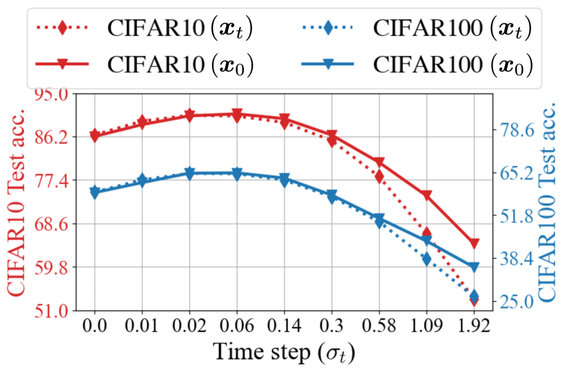
(a) Classification

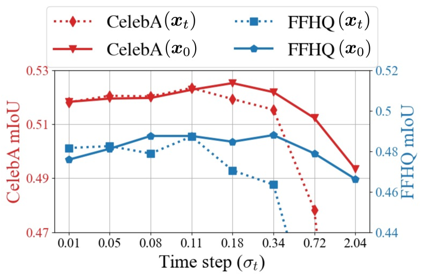
(b) Segmentation

Figure 1: Unimodal representation dynamic: using clean images as inputs improves representation quality. We train DDPM/EDM-based diffusion models on various datasets and evaluate downstream performance using clean images ($\bm{x}_{0}$) versus noisy images ($\bm{x}_{t}$). Both scenarios show a unimodal performance trend, peaking at intermediate noise levels. While clean images perform similarly to noisy inputs at low noise, they outperform as noise increases.

2.1 Preliminaries on Denoising Diffusion Models

Basics of diffusion models.

Diffusion models are a class of probabilistic generative models that aim to reverse a progressive noising process by mapping an underlying data distribution, $p_{\text{data}}$, to a Gaussian distribution.

• The forward diffusion process. Starting from clean data $\bm{x}_{0}$, noise is progressively added following a schedule based on time step $t$ until the data becomes pure Gaussian noise. At each step $t$, the noised data is expressed as $\bm{x}_{t}=s_{t}\bm{x}_{0}+s_{t}\sigma_{t}\bm{\epsilon}$, where $\bm{\epsilon}\sim\mathcal{N}(\bm{0},\bm{I})$ is Gaussian noise, and $s_{t}$, $s_{t}\sigma_{t}$ scale the signal and noise, respectively.

• The reverse diffusion process. We can run a reverse SDE (Anderson, 1982) to sample from $\bm{x}_{1}$ as:

  $$\mathrm{d}\bm{x}_{t}=\left(f(t)\bm{x}_{t}-g^{2}(t)\nabla\log p_{t}(\bm{x}_{t})\right)\mathrm{d}t+g(t)\mathrm{d}\bar{\bm{w}}_{t},$$

  where $\{\bar{\bm{w}_{t}}\}_{t\in[0,1]}$ is the standard Wiener process running backward in time from $t=1$ to $t=0$ and the functions $f(t),g(t):\mathbb{R}\to\mathbb{R}$ respectively denote the drift and diffusion coefficients.

Training with denoising auto-encoder (DAE) based objective.

Since the score function $\nabla\log p_{t}(\bm{x}_{t})$ depends on the unknown data distribution $p_{\rm data}$ and satisfies

$$s_{t}\operatorname{\mathbb{E}}\left[\bm{x}_{0}|\bm{x}_{t}\right]=\bm{x}_{t}+s_{t}^{2}\sigma_{t}^{2}\nabla\log p_{t}(\bm{x}_{t}),$$ (1)

we can estimate $\nabla\log p_{t}(\bm{x}_{t})$ by training a network $\bm{x}_{\bm{\theta}}(\bm{x}_{t},t)$ to approximate the posterior mean $\operatorname{\mathbb{E}}[\bm{x}_{0}|\bm{x}_{t}]$ (Chen et al., 2024b; Xiang et al., 2023; Kadkhodaie et al., 2024). This is achieved by minimizing the loss $\mathcal{L}(\bm{\theta})$ via

$$\min_{\bm{\theta}}\;\sum_{i=1}^{N}\int_{0}^{1}\lambda_{t}\operatorname{\mathbb{E}}_{\bm{\epsilon}}\left[\left\|\bm{x}_{\bm{\theta}}(\bm{x}_{t}^{(i)},t)-\bm{x}_{0}^{(i)}\right\|^{2}\right]\mathrm{d}t,$$ (2)

where $\bm{\epsilon}\sim\mathcal{N}(\bm{0},\bm{I}_{n})$, $\lambda_{t}$ represents the weight associated with each noise level, and $N$ denotes the dataset size. Moreover, $\bm{x}_{i}^{(0)}\overset{i.i.d.}{\sim}p_{\rm data}$ is the training sample and the corresponding noisy sample is given by $\bm{x}_{t}^{(i)}=s_{t}\bm{x}_{0}^{(i)}+s_{t}\sigma_{t}\bm{\epsilon}$ for each $i\in[N]$. To simplify the analysis, we assume throughout the paper that $s_{t}=1$ and $\lambda_{t}$ remain constant across all noise levels, with the noise level denoted as $\sigma_{t}$. It is worth noting if we only minimize the error at one specific timestep, we are exactly training a single step DAE proposed in (Vincent, 2011), and in Section˜4.2 we discuss the superiority of diffusion models over DAEs.

2.2 Representation Learning via Diffusion Models

Once the diffusion model $\bm{x}_{\bm{\theta}}$ is trained via (2), we extract and evaluate the representation from data $\bm{x}_{0}$ as follows:

• Using clean images as network inputs. We propose to use clean images, $\bm{x}_{0}$, as inputs to the network $\bm{x}_{\bm{\theta}}(\bm{x}_{0},t)$ for extracting representation across different noise levels $t$. This is different from existing approaches (Xiang et al., 2023; Baranchuk et al., 2022; Tang et al., 2023) that use noisy images $\bm{x}_{t}$ for representation extraction.

• Layer selection for representations. Following the protocol in (Xiang et al., 2023), we freeze the entire model and extract representations from the layer of the diffusion model $\bm{x}_{\bm{\theta}}(\bm{x}_{0},t)$ that yields the best downstream performance. Typically, we select a layer near the bottleneck layer of U-Net and the exact midpoint layer of DiT to balance between data compression and performance.

• Evaluation of representation. Once the model is trained, we freeze the model and assess its representation quality based on downstream performance metrics, such as accuracy for classification and mean intersection over union (mIoU) for segmentation tasks.

Remarks on network inputs.

Beyond simplifying the analysis, our choice of using clean images as network inputs $\bm{x}_{\bm{\theta}}(\bm{x}_{0},t)$ (rather than $\bm{x}_{\bm{\theta}}(\bm{x}_{t},t)$) for representation extraction is driven by two primary considerations.

• Empirical performance gains. As demonstrated in Figure˜1, using clean inputs outperforms using noisy inputs $\bm{x}_{t}$ on both classificaiton and segmentation tasks, a result further supported by our studies on the posterior estimation; see Figure˜10 in the Appendix. These findings imply that the denoising objective is the primary driver of representation capabilities in diffusion models, whereas the progressive denoising procedure has a relatively minor impact on representation quality.

• Alignment with existing learning paradigms. Moreover, our approach is also consistent with standard supervised and self-supervised learning, where data augmentations (e.g., cropping (Caron et al., 2021), color jittering, masking (He et al., 2022)) are applied during training to improve robustness, but clean, unaugmented images are typically used at inference. In diffusion models, similarly, additive Gaussian noise serves as a form of data augmentation during training (Chen et al., 2024b), while clean images are used for inference.

3 Study of Representation Dynamics

With the setup in Section˜2, this section theoretically investigates the representation dynamics of diffusion models across the noise levels, providing new insights for understanding the representation-generation tradeoff. Moreover, our theoretical studies are corroborated by experimental results on real datasets.

3.1 Assumptions of Low-Dimensional Data Distribution

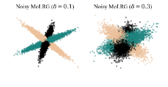
Figure 2: An illustration of MoLRG with different noise levels. We visualize samples drawn from noisy MoLRG with noise levels $\delta=0.1,\;0.3$ and $K=3$.

In this work, we assume that the input data follows a noisy version of the mixture of low-rank Gaussians (MoLRG) distribution (Wang et al., 2024; Elhamifar and Vidal, 2013; Wang et al., 2022), defined as follows.

Assumption 1 ($K$-Class Noisy MoLRG Distribution).

For any sample $\bm{x}_{0}$ drawn from the noisy MoLRG distribution with $K$ subspaces, the following holds:

$$\bm{x}_{0}=\bm{U}_{k}\bm{a}+\delta\bm{U}_{k}^{\perp}\bm{e},\;\text{with prob.}\;\pi_{k}\geq 0,\;k\in[K].$$ (3)

Here, $k$ represents the class of $\bm{x}_{0}$ and follows a multinomial distribution $k\sim\text{Mult}(K,\pi_{k})$, $\bm{U}_{k}\in\mathcal{O}^{n\times d_{k}}$ denotes an orthonormal basis for the $k$-th subspace with its complement $\bm{U}_{k}^{\perp}\in\mathcal{O}^{n\times(n-d_{k})}$, $d_{k}$ is the subspace dimension with $d_{k}\ll n$, and the coefficient $\bm{a}\overset{i.i.d.}{\sim}\mathcal{N}(\bm{0},\bm{I}_{d_{k}})$ is drawn from the normal distribution. The level of the noise $\bm{e}\overset{i.i.d.}{\sim}\mathcal{N}(\bm{0},\bm{I}_{n-d_{k}})$ is controlled by the scalar $\delta<1$.

As shown in Figure˜2, data from MoLRG resides on a union of low-dimensional subspaces, each following a Gaussian distribution with a low-rank covariance matrix representing its basis. The study of Noisy MoLRG  distributions is further motivated by the fact that

• MoLRG captures the intrinsic low-dimensionality of image data. Although real-world image datasets are high-dimensional in terms of pixel count and data volume, extensive empirical studies (Gong et al., 2019; Pope et al., 2021; Stanczuk et al., 2022) demonstrated that their intrinsic dimensionality is considerably lower. Additionally, recent work (Huang et al., 2024; Liang et al., 2025) has leveraged the intrinsic low-dimensional structure of real-world data to analyze the convergence guarantees of diffusion model sampling. The MoLRG distribution, which models data in a low-dimensional space with rank $d_{k}\ll n$, effectively captures this property.

• The latent space of latent diffusion models is approximately Gaussian. State-of-the-art large-scale diffusion models (Peebles and Xie, 2023; Podell et al., 2024) typically employ autoencoders (Kingma, 2013) to project images into a low-dimensional latent space, where a KL penalty encourages the learned latent distribution to approximate standard Gaussians (Rombach et al., 2022). Furthermore, recent studies (Jing et al., 2022; Chen et al., 2024b) show that diffusion models can be trained to leverage the intrinsic subspace structure of real-world data.

• Modeling the complexity of real-world image datasets. The noise term $\delta\bm{U}_{k}^{\perp}\bm{e}_{i}$ captures perturbations outside the $k$-th subspace via the orthogonal complement $\bm{U}_{k}^{\perp}$, analogous to insignificant attributes of real-world images, such as the background of an image. While this additional noise term may be less significant for representation learning, it plays a crucial role in enhancing the fidelity of generated samples.

Moreover, the noisy MoLRG  is analytically tractable. For simplicity, we assume equal subspace dimensions ($d_{1}=\dots=d_{K}=d$), orthogonal bases ($\bm{U}_{k}^{T}\bm{U}_{l}=\bm{0}$ for $k\neq l$), uniform mixing weights ($\pi_{1}=\dots=\pi_{K}=1/K$), and define the noise space as $\bm{U}_{\perp}=\bigcap_{k=1}^{K}\bm{U}_{k}^{\perp}\in\mathcal{O}^{n\times(n-Kd)}$. Then, we can derive the ground truth posterior mean $\operatorname{\mathbb{E}}\left[\bm{x}_{0}|\bm{x}_{t}\right]$ for the noisy MoLRG  distribution as:

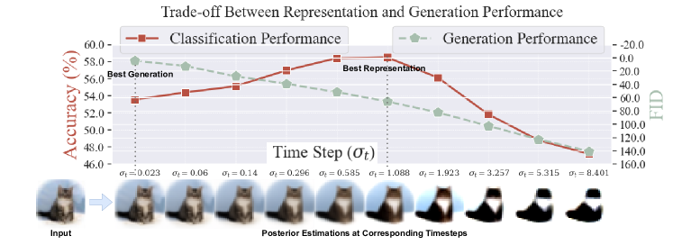
Figure 3: Trade-offs between representation quality and generation quality. The curve with pentagon markers demonstrates the transition from fine to coarse granularity in posterior estimation as noise levels increase, corresponding to the monotonic rise in FID. In contrast, the curve with square markers reveals an unimodal trend in posterior classification accuracy, achieving peak performance at intermediate noise levels. This occurs when high-level details are filtered out while essential low-level semantic information is preserved, as illustrated by the posterior estimations according to different noise levels shown at the bottom of the figure.

Proposition 1.

Suppose the data $\bm{x}_{0}$ is drawn from a noisy MoLRG data distribution with $K$-class and noise level $\delta$. Let $\zeta_{t}=\frac{1}{1+\sigma_{t}^{2}}$ and $\xi_{t}=\frac{\delta^{2}}{\delta^{2}+\sigma_{t}^{2}}$, where $\sigma_{t}$ is the noise scaling in (1). Then for each time $t>0$, the optimal posterior estimator $\operatorname{\mathbb{E}}\left[\bm{x}_{0}|\bm{x}_{t}\right]$ has the analytical form:

$$\operatorname{\mathbb{E}}\left[\bm{x}_{0}|\bm{x}_{t}\right]=\sum_{l=1}^{K}w^{\star}_{l}(\bm{x}_{t},t)\left(\zeta_{t}\bm{U}_{l}\bm{U}_{l}^{T}+\xi_{t}\bm{U}_{l}^{\perp}\bm{U}_{l}^{\perp T}\right)\bm{x}_{t}.$$

where $w^{\star}_{l}(\bm{x}_{t},t)=\frac{\exp\left(g_{l}(\bm{x}_{t},t)\right)}{\sum_{l=1}^{K}\exp\left(g_{l}(\bm{x}_{t},t)\right)}$ is a soft-max operator for $g_{l}(\bm{x},t)=\frac{1}{2\sigma_{t}^{2}}\zeta_{t}\|\bm{U}_{l}^{T}\bm{x}\|^{2}+\frac{\delta^{2}}{2\sigma_{t}^{2}}\xi_{t}\|\bm{U}_{l}^{\perp T}\bm{x}\|^{2}$.

The proof can be found in Section˜A.4.1 and it is an extension of the result in (Wang et al., 2024). For $\bm{x}_{0}$ following noisy MoLRG, note that the optimal solution $\hat{\bm{x}}_{\bm{\theta}}^{\star}(\bm{x}_{t},t)$ of the training loss (2) would exactly be $\operatorname{\mathbb{E}}\left[\bm{x}_{0}|\bm{x}_{t}\right]$. As such, as illustrated in Figure˜3, the analytical form of the posterior estimation facilitates the study of generation-representation tradeoff across timesteps:

• The generation quality. The generation quality of posterior estimation cam be measured by $||\hat{\bm{x}}_{\bm{\theta}}^{\star}(\bm{x}_{t},t)-\bm{x}_{0}||^{2}$. As shown in ˜1, this error is minimized at $t=0$ with $\sigma_{t}=0$, where the true class weight satisfies $w^{\star}_{k}(\bm{x}_{t})=1$, yielding $\hat{\bm{x}}_{\bm{\theta}}^{\star}(\bm{x}_{t},t)=\bm{x}_{0}$. As $t$ increases, higher noise levels $\sigma_{t}$ decrease $w^{\star}_{k}(\bm{x}_{t})$, causing a monotonic increase in FID, as seen in Figure˜3.

• The representation quality. The representation quality follows a unimodal trend across timesteps (Xiang et al., 2023; Tang et al., 2023), which can be measured through the posterior estimator $\hat{\bm{x}}_{\bm{\theta}}^{\star}(\bm{x}_{t},t)$ (see Section˜3.2). As shown in Figure˜3, this unimodal behavior creates a trade-off between generation and representation quality, particularly at smaller $t$ when closer to the original image.

3.2 Measuring Posterior Representation Quality

For understanding diffusion-based representation learning, we introduce a metric termed Class-specific Signal-to-Noise Ratio ($\mathrm{CSNR}$) to quantify the posterior representation quality as follows.

Definition 1 (Class-specific Signal-to-Noise Ratio).

Suppose the data $\bm{x}_{0}$ follows the noisy MoLRG introduced in ˜1. Without loss of generality, let $k$ denote the true class of $\bm{x}_{0}$. For its associated posterior estimator $\hat{\bm{x}}_{\bm{\theta}}$,

$$\mathrm{CSNR}(\hat{\bm{x}}_{\bm{\theta}},t):=\operatorname{\mathbb{E}}_{k}\left[\frac{\operatorname{\mathbb{E}}_{\bm{x}_{0}}[\|\bm{U}_{k}\bm{U}_{k}^{T}\hat{\bm{x}}_{\bm{\theta}}(\bm{x}_{0},t)\|^{2}\mid k]}{\operatorname{\mathbb{E}}_{\bm{x}_{0}}[\sum_{l\neq k}\|\bm{U}_{l}\bm{U}_{l}^{T}\hat{\bm{x}}_{\bm{\theta}}(\bm{x}_{0},t)\|^{2}\mid k]}\right]$$

Here, $\bm{U}_{k}$ represents the basis of the subspace corresponding to the true class to which $\bm{x}_{0}$ belongs and the $\bm{U}_{l}$s with $l\neq k$ denotes the bases of the subspaces for other classes.

Intuitively, successful prediction of the class for $\bm{x}_{0}$ is achieved when the projection onto the correct class subspace, $\|\bm{U}_{k}\bm{U}_{k}^{T}\hat{\bm{x}}_{\bm{\theta}}(\bm{x}_{0},t)\|$, preserves larger energy than the projections onto subspaces of any other class, $\|\bm{U}_{l}\bm{U}_{l}^{T}\hat{\bm{x}}_{\bm{\theta}}(\bm{x}_{0},t)\|$. Thus, $\mathrm{CSNR}$ measures the ratio of the true class signal to irrelevant noise from other classes at a given noise level $t$, serving as a practical metric for evaluating classification performance and hence the representation quality. In this work, we use posterior representation quality as a proxy for studying the representation dynamics of diffusion models for the following reasons:

• Posterior quality reflects feature quality. Diffusion models $\hat{\bm{x}}_{\bm{\theta}}$ are trained to perform posterior estimation at a given time step $t$ using corrupted inputs, with the intermediate features emerging as a byproduct of this process. Thus, a more class-representative posterior estimation inherently implies more class-representative intermediate features.

• Model-agnostic analysis. Our goal is to provide a general analysis independent of specific network architectures and feature extraction protocols. Posterior representation quality offers a unified metric that avoids assumptions tied to particular architectures, making the analysis broadly applicable.

3.3 Main Theoretical Results

Based upon the setup in Section˜3.1 and Section˜3.2, we obtain the following results.

Theorem 1.

(Informal) Suppose the data $\bm{x}_{0}$ follows the noisy MoLRG introduced in ˜1 with $K$ classes and noise level $\delta$, then the $\mathrm{CSNR}$ of the optimal denoiser $\hat{\bm{x}}_{\theta}^{\star}$ takes the following form:

$$\mathrm{CSNR}(\hat{\bm{x}}_{\theta}^{\star},t)=\frac{1}{(K-1)\delta^{2}}\cdot\left(\frac{1+\frac{\sigma_{t}^{2}}{\delta^{2}}h(\hat{w}_{t}^{+},\delta)}{1+\frac{\sigma_{t}^{2}}{\delta^{2}}h(\hat{w}_{t}^{-},\delta)}\right)^{2}.$$ (4)

Here, $h(w,\delta):=(1-\delta^{2})w+\delta^{2}$ is a monotonically increasing function with respect to $w$. Additionally, $h(\hat{w}_{t}^{+},\delta)$ and $h(\hat{w}_{t}^{-},\delta)$ denote positive and negative class confidence rates with

$$\begin{cases}\hat{w}_{t}^{+}(\sigma_{t},\delta)&=\;\mathbb{E}_{k}[\mathbb{E}_{\bm{x}_{0}}[w_{k}(\bm{x}_{0},t)\mid k]],\\ \hat{w}_{t}^{-}(\sigma_{t},\delta)&=\;\mathbb{E}_{k}[\mathbb{E}_{\bm{x}_{0}}[w_{l}(\bm{x}_{0},t)\mid k\neq l]],\end{cases}$$

whose analytical forms can be found in Section˜A.4.2.

We defer the formal statement of Theorem˜1 and its proof to Section˜A.4.2. In the following, we discuss the implications of our result.

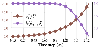
Figure 4: Illustration of the interplay between the denoising rate and the class confidence rate.

The unimodal curve of $\mathrm{CSNR}$ across noise levels.

Intuitively, our theorem shows that unimodal curve is mainly induced by the the interplay between the “denoising rate" $\sigma_{t}^{2}/\delta^{2}$ and the positive class confidence rate $h(\hat{w}_{t}^{+},\delta)$ as noise level $\sigma_{t}$ increases. As observed in Figure˜4, the “denoising rate" ($\sigma_{t}^{2}/\delta^{2}$) increases monotonically with $\sigma_{t}$ while the class confidence rate $h(\hat{w}_{t}^{+},\delta)$ monotonically declines. Initially, when $\sigma_{t}$ is small, the class confidence rate remains relatively stable due to its flat slope, and an increasing “denoising rate" improves the $\mathrm{CSNR}$, resulting in improved posterior estimation. However, as indicated by ˜1, when $\sigma_{t}$ becomes too large, $h(\hat{w}_{t}^{+},\delta)$ approaches $h(\hat{w}_{t}^{-},\delta)$, leading to a drop in $\mathrm{CSNR}$, which limits the ability of the model to project $\bm{x}_{0}$ onto the correct signal subspace and ultimately hurts posterior estimation.

Alignment of $\mathrm{CSNR}$ with posterior representation quality.

Although our theory is derived from the noisy MoLRG  distribution, it effectively captures real-world phenomena. As shown in Figures˜5 and 6, we conduct experiments on both synthetic (i.e., noisy MoLRG) and real-world datasets (i.e., CIFAR and ImageNet) to measure $\mathrm{CSNR}(\hat{\bm{x}}_{\bm{\theta}},t)$ as well as the posterior probing accuracy. For posterior probing, we use posterior estimations at different timesteps as inputs for classification. The results consistently show that $\mathrm{CSNR}(\hat{\bm{x}}_{\bm{\theta}},t)$ follows a unimodal pattern across all cases, mirroring the trend observed in posterior probing accuracy as the noise scale increases. This alignment provides a formal justification for previous empirical findings (Xiang et al., 2023; Baranchuk et al., 2022; Tang et al., 2023), which have reported a unimodal trajectory in the representation dynamics of diffusion models with increasing noise levels. Detailed experimental setups are provided in Section˜A.3.

Explanation of generation and representation trade-off.

Our theoretical findings reveal the underlying rationale behind the generation and representation trade-off: the proportion of data associated with $\delta$ represents class-irrelevant attributes. The unimodal representation learning dynamic thus captures a “fine-to-coarse" shift (Choi et al., 2022; Wang and Vastola, 2023), where these class-irrelevant attributes are progressively stripped away. During this process, peak representation performance is achieved at a balance point where class-irrelevant attributes are eliminated, while class-essential information is preserved. In contrast, high-fidelity image generation requires capturing the entire data distribution—from coarse structures to fine details—leading to optimal performance at the lowest noise level $\sigma_{t}$, where class-irrelevant attributes encoded in the $\delta$-term are maximally retained. Thus, our insights explain the trade-off between generation and representation quality. As visualized in Figure˜3 and Figure˜15, representation quality peaks at an intermediate noise level where irrelevant details are stripped away, while generation quality peaks at the lowest noise level, where all details are preserved.

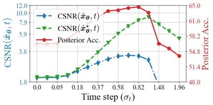
Figure 5: Posterior probing accuracy and associated $\mathrm{CSNR}$ dynamics in MoLRG data. We plot the posterior probing accuracy and $\mathrm{CSNR}$ with the posterior estimations obtained from a learned estimator $\bm{\hat{x}_{\theta}}$. both of which exhibit a consistent unimodal pattern. Additionally, we include the optimal $\mathrm{CSNR}$ , calculated from the ground truth posterior function $\bm{\hat{x}_{\theta}}^{\star}$ defined in ˜1, as a reference. The estimator is trained on a 3-class MoLRG dataset with data dimension $n=50$, subspace dimension $d=15$, and noise scale $\delta=0.5$.

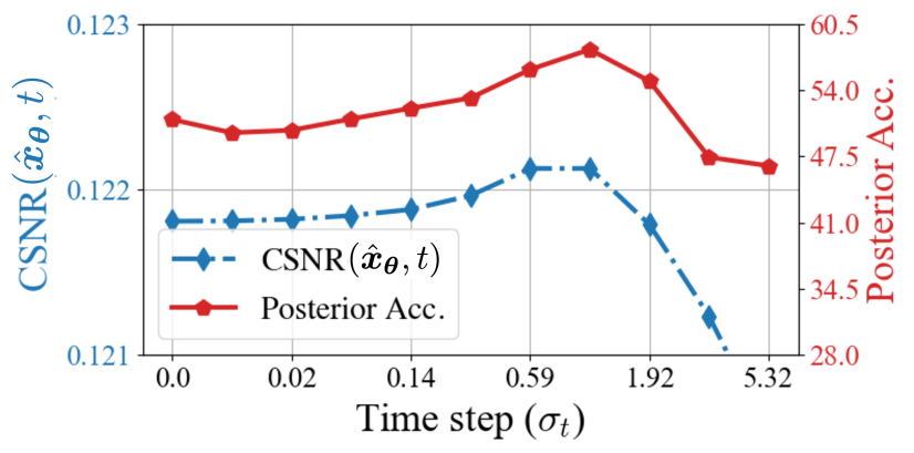
(a) CIFAR10

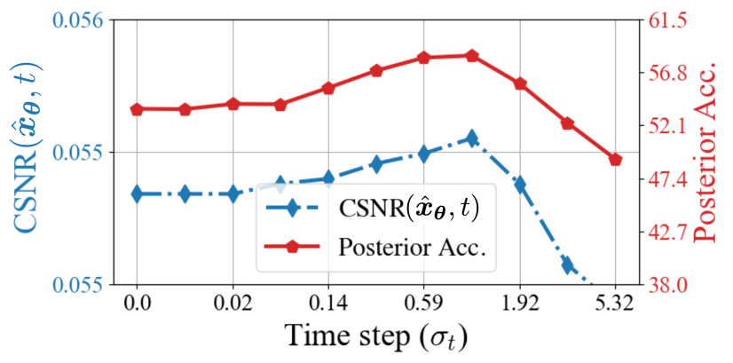
(b) MiniImageNet

Figure 6: Dynamics of posterior probing accuracy and associated $\mathrm{CSNR}$ on CIFAR10 and MiniImageNet. Posterior probing accuracy is plotted alongside $\mathrm{CSNR}(\hat{\bm{x}}_{\bm{\theta}},t)$. Probing accuracy is evaluated on the test set, while the empirical $\mathrm{CSNR}$ is computed from the training set. Both exhibit an aligning unimodal pattern. We use released EDM models (Karras et al., 2022) trained on the CIFAR-10 (Krizhevsky et al., 2009) and ImageNet (Deng et al., 2009) datasets, evaluating them on CIFAR-10 and MiniImageNet (Vinyals et al., 2016), respectively. To compute $\mathrm{CSNR}$ , we apply PCA on the original CIFAR-10/MiniImageNet images to extract the basis $\bm{U}_{k}$s. Further details can be found in Section˜A.3.

4 Practical Insights

We examine the practical implications of our findings in Section˜4.1, leveraging feature information at different levels of granularity to enhance robustness. Additionally, we discuss the advantages of diffusion models over traditional single-step DAEs in Section˜4.2.

4.1 Feature Ensembling Across Timesteps Improves Representation Robustness

Our theoretical insights imply that features extracted at different timesteps capture varying levels of granularity. Given the high linear separability of intermediate features, we propose a simple ensembling approach across multiple timesteps to construct a more holistic representation of the input. Specifically, in addition to the optimal timestep, we extract feature representations at four additional timesteps—two from the coarse (larger $\sigma_{t}$) and two from the fine-grained (smaller $\sigma_{t}$) end of the spectrum. We then train linear probing classifiers for each set and, during inference, apply a soft-voting ensemble by averaging the predicted logits before making a final decision.(experiment details in Section˜A.3)

We evaluate this ensemble method against results obtained from the best individual timestep, as well as a self-supervised method MAE (He et al., 2022), on both the pre-training dataset and a transfer learning setup. The results, reported in Table˜1 and Table˜2, demonstrate that ensembling significantly enhances performance for both EDM (Karras et al., 2022) and DiT (Peebles and Xie, 2023), consistently outperforming their vanilla diffusion model counterparts and often surpassing MAE. Moreover, ensembling substantially improves the robustness of diffusion models for classification under label noise.

Method	MiniImageNet⋆ Test Acc. %
Label Noise	Clean	20%	40%	60%	80%
MAE	73.7	70.3	67.4	62.8	51.5
EDM	67.2	62.9	59.2	53.2	40.1
EDM (Ensemble)	72.0	67.8	64.7	60.0	48.2
DiT	77.6	72.4	68.4	62.0	47.3
DiT (Ensemble)	78.4	75.1	71.9	66.7	56.3

Table 1: Comparison of test performance across different methods under varying label noise levels. All compared models are publicly available and pre-trained on ImageNet-1K (Deng et al., 2009), evaluated using MiniImageNet classes. Bold font highlights the best result in each scenario.

Method	Transfer Test Acc. %
	CIFAR100					DTD					Flowers102
Label Noise	Clean	20%	40%	60%	80%	Clean	20%	40%	60%	80%	Clean	20%	40%	60%	80%
MAE	63.0	58.8	54.7	50.1	38.4	61.4	54.3	49.9	40.5	24.1	68.9	55.2	40.3	27.6	9.6
EDM	62.7	58.5	53.8	48.0	35.6	54.0	49.1	45.1	36.4	21.2	62.8	48.2	37.2	24.1	9.7
EDM (Ensemble)	67.5	64.2	60.4	55.4	43.9	55.7	49.5	45.2	37.1	22.0	67.8	53.9	41.5	25.0	10.4
DiT	64.2	58.7	53.5	46.4	32.6	65.2	59.7	53.0	43.8	27.0	78.9	65.2	52.4	34.7	13.3
DiT (Ensemble)	66.4	61.8	57.6	51.3	39.2	65.3	60.6	56.1	46.3	30.6	79.7	67.0	54.6	36.6	14.7

Table 2: Comparison of transfer learning performance across different methods under varying label noise levels. All compared models are publicly available and pre-trained on ImageNet-1K (Deng et al., 2009), evaluated on different downstream datasets. Bold font highlights the best result in each scenario.

4.2 Weight Sharing in Diffusion Models Facilitates Representation Learning

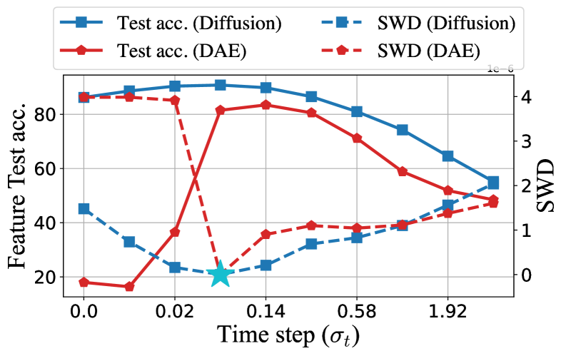
(a) CIFAR10

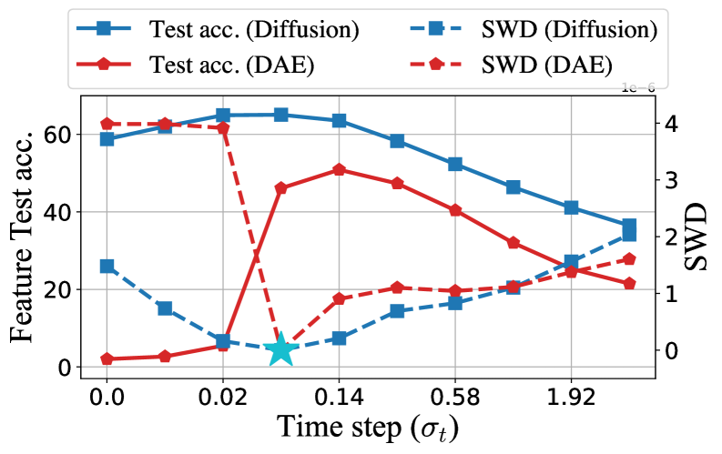
(b) CIFAR100

Figure 7: Diffusion models exhibit higher and smoother feature accuracy and similarity compared to individual DAEs. We train DDPM-based diffusion models and individual DAEs on the CIFAR datasets and evaluate their representation learning performance. Feature accuracy, and feature differences from the optimal features (indicated by $\star$) are plotted against increasing noise levels. The results reveal an inverse correlation between feature accuracy and feature differences, with diffusion models achieving both higher/smoother accuracy and smaller/smoother feature differences compared to DAEs.

Second, we reveal why diffusion models, despite sharing the same denoising objective with classical DAEs, achieve superior representation learning due to their inherent weight-sharing mechanism. By minimizing loss across all noise levels (2), diffusion models enable parameter sharing and interaction among denoising subcomponents, creating an implicit "ensemble" effect. This improves feature consistency and robustness across noise scales compared to DAEs (Chen et al., 2024b), as illustrated in Figure˜7.

To test this, we trained 10 DAEs, each specialized for a single noise level, alongside a DDPM-based diffusion model on CIFAR10 and CIFAR100. We compared feature quality using linear probing accuracy and feature similarity relative to the optimal features at $\sigma_{t}=0.06$ (where accuracy peaks) via sliced Wasserstein distance ($\mathrm{SWD}$) (Doan et al., 2024).

The results in Figure˜7 confirm the advantage of diffusion models over DAEs. Diffusion models consistently outperform DAEs, particularly in low-noise regimes where DAEs collapse into trivial identity mappings. In contrast, diffusion models leverage weight-sharing to preserve high-quality features, ensuring smoother transitions and higher accuracy as noise increases. This advantage is further supported by the $\mathrm{SWD}$ curve, which reveals an inverse correlation between feature accuracy and feature differences. Notably, diffusion model features remain significantly closer to their optimal state across all noise levels, demonstrating superior representational capacity.

Our finding also aligns with prior results that sequentially training DAEs across multiple noise levels improves representation quality (Chandra and Sharma, 2014; Geras and Sutton, 2015; Zhang and Zhang, 2018). Our ablation study further confirms that multi-scale training is essential for improving DAE performance on classification tasks in low-noise settings (details in Section˜A.2, Table˜3).

5 Discussion

In this work, we develop a mathematical framework for analyzing the representation dynamics of diffusion models. By introducing the concept of $\mathrm{CSNR}$ and leveraging a low-dimensional mixture of low-rank Gaussians, we characterize the trade-off between generative quality and representation quality. Our theoretical analysis explains how the unimodal representation learning dynamics observed across noise scales emerge from the interplay between data denoising and class specification.

Beyond theoretical insights, we propose an ensemble method inspired by our findings that enhances classification performance in diffusion models, both with and without label noise. Additionally, we empirically uncover an inherent weight-sharing mechanism in diffusion models, which accounts for their superior representation quality compared to traditional DAEs. Experiments on both synthetic and real-world datasets validate our findings. Additionally, our findings also open up new avenues for future research that we discuss in the following.

• Principled diffusion-based representation learning. While diffusion models have shown strong performance in various representation learning tasks, their application often relies on trial-and-error methods and heuristics. For example, determining the optimal layer and noise scale for feature extraction frequently involves grid searches. Our work provides a theoretical framework to understand representation dynamics across noise scales. A promising future direction is to extend this analysis to include layer-wise dynamics. Combining these insights could pave the way for more principled and efficient approaches to diffusion-based representation learning.

• Representation alignment for better image generation. Recent work REPA Yu et al. (2024) has demonstrated that aligning diffusion model features with features from pre-trained self-supervised foundation models can enhance training efficiency and improve generation quality. By providing a deeper understanding of the representation dynamics in diffusion models, our findings could further advance such representation alignment techniques, facilitating the development of diffusion models with superior training and generation performance.

Acnkowledgement

We acknowledge funding support from NSF CAREER CCF-2143904, NSF CCF-2212066, NSF CCF- 2212326, NSF IIS 2312842, NSF IIS 2402950, ONR N00014-22-1-2529, and MICDE Catalyst Grant.

Appendix A Appendix

The Appendix is organized as follows: in Section˜A.1, we discuss related works; in Section˜A.2, we provide complementary experiments; in Section˜A.3, we present the detailed experimental setups for the empirical results in the paper. Lastly, in Section˜A.4, we provide proof details for Section˜3.

A.1 Related Works

Denoising auto-encoders.

Denoising autoencoders (DAEs) are trained to reconstruct corrupted images to extract semantically meaningful information, which can be applied to various vision [Vincent et al., 2008, 2010] and language downstream tasks [Lewis et al., 2020]. Related to our analysis of the weight-sharing mechanism, several studies have shown that training with a noise scheduler can enhance downstream performance [Chandra and Sharma, 2014, Geras and Sutton, 2015, Zhang and Zhang, 2018]. On the theoretical side, prior works have studied the learning dynamics [Pretorius et al., 2018, Steck, 2020] and optimization landscape [Kunin et al., 2019] through the simplified linear DAE models.

Diffusion-based representation learning.

Diffusion-based representation learning [Fuest et al., 2024] has demonstrated significant success in various downstream tasks, including image classification [Xiang et al., 2023, Mukhopadhyay et al., 2023, Deja et al., 2023], segmentation [Baranchuk et al., 2022], correspondence [Tang et al., 2023], and image editing [Shi et al., 2024]. To further enhance the utility of diffusion features, knowledge distillation [Yang and Wang, 2023, Li et al., 2023, Stracke et al., 2024, Luo et al., 2024] methods have been proposed, aiming to bypass the computationally expensive grid search for the optimal $t$ in feature extraction and improving downstream performance. Beyond directly using intermediate features from pre-trained diffusion models, research efforts has also explored novel loss functions [Abstreiter et al., 2021, Wang et al., 2023] and network modifications [Hudson et al., 2024, Preechakul et al., 2022] to develop more unified generative and representation learning capabilities within diffusion models. Unlike the aforementioned efforts, our work focuses more on understanding the representation learning capabilities of diffusion models.

A.2 Additional Experiments

Influence of data complexity in diffusion representation learning

Our analyses in the main body of the paper are based on the assumption that the training dataset contains sufficient samples for the diffusion model to learn the underlying distribution. Interestingly, if this assumption is violated by training the model on insufficient data, the unimodal representation learning dynamic disappears and the probing accuracy also drops severely.

As illustrated in Figure˜8, we train $2$ different UNets following the EDM [Karras et al., 2022] configuration with training dataset size ranging from $2^{5}$ to $2^{15}$. The unimodal curve emerges only when the dataset size exceeds $2^{12}$, whereas smaller datasets produce flat curves.

The underlying reason for this observation is that, when training data is limited, diffusion models memorize all individual data points rather than learn the true underlying data structure [Wang et al., 2024]. In this scenario, the model memorizes an empirical distribution that lacks meaningful low-dimensional structures and thus deviates from the setting in our theory, leading to the loss of the unimodal representation dynamic. To confirm this, we calculated the generalization score, which measures the percentage of generated data that does not belong to the training dataset, as defined in [Zhang et al., 2023]. As shown in Figure˜9, representation learning only achieves strong accuracy and displays the unimodal dynamic when the generalization score approaches $1$, aligning with our theoretical assumptions.

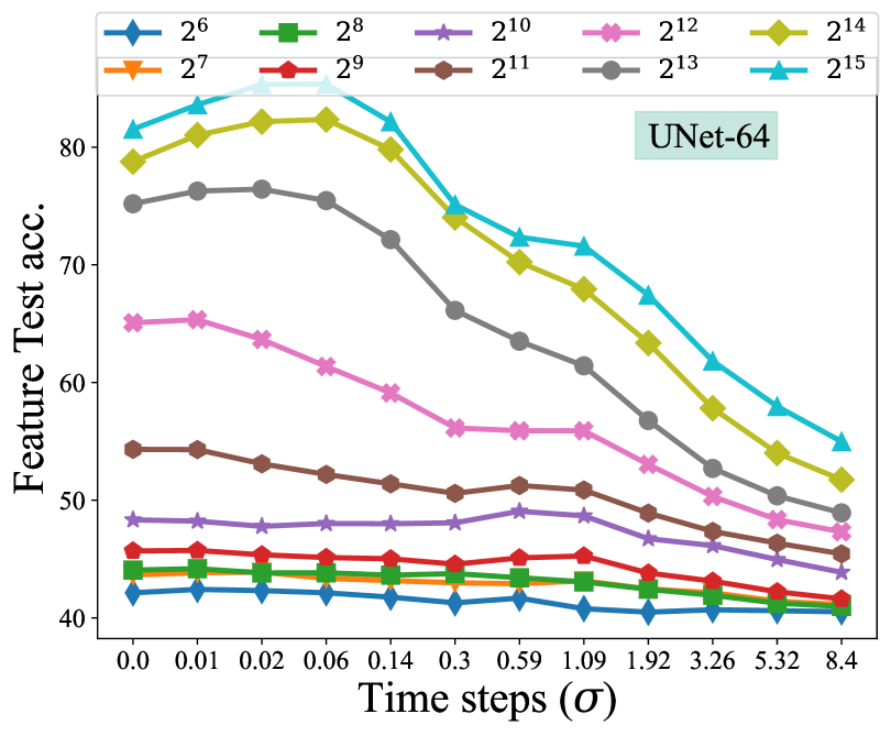
(a) UNet-64 accuracy trend

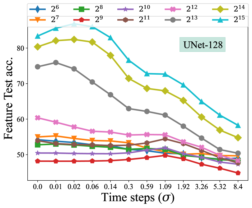
(b) UNet-128 accuracy trend

Figure 8: The influence of data complexity in diffusion-based representation learning. With the same model trained in Figure˜9, we plot the representation learning dynamics for each trained model as a function of changing noise levels.

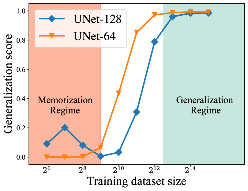
(a) Phase transition in generalization score

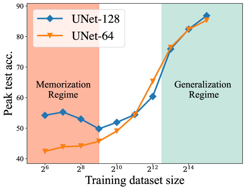
(b) Phase transition in representation learning

Figure 9: Better representations are learned in the generalization regime. We train EDM-based [Karras et al., 2022] diffusion models on the CIFAR-10 dataset using different training dataset sizes, ranging from $2^{6}$ to $2^{15}$. (a) The change in the generalization score [Zhang et al., 2023] as the dataset size increases, where regions with a generalization score close to $0$ are labeled as the memorization regime, and those close to $1$ are labeled as the generalization regime. (b) The peak representation learning feature accuracy achieved as a function of dataset size.

Posterior quality decides feature quality

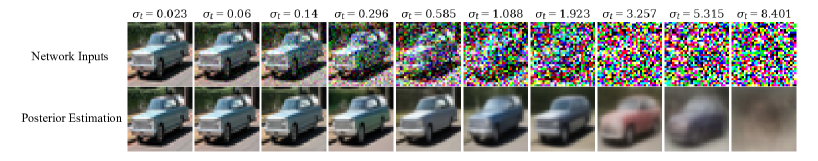
(a) $\hat{\bm{x}}_{\bm{\theta}}(\bm{x}_{t},t)$: Posterior estimation using noise image as inputs.

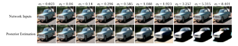
(b) $\hat{\bm{x}}_{\bm{\theta}}(\bm{x}_{0},t)$: Posterior estimation using clean image as inputs.

Figure 10: Using clean images as inputs improves posterior estimation quality. We use a pre-trained DDPM diffusion model on CIFAR10 to visualize posterior estimation for clean inputs and noisy inputs across varying noise scales $\sigma_{t}$. Clean inputs produce smooth and descriptive estimations even at high noise levels, whereas noisy inputs result in blurry and lossy estimations at large $\sigma_{t}$, making it difficult to extract meaningful representations.

Diffusion models $\hat{\bm{x}}_{\bm{\theta}}$ are trained to perform posterior estimation at a given time step $t$ using corrupted inputs, with the features for representation learning emerging as an intermediate byproduct of this process. This leads to a natural conjecture: changes in feature quality should directly correspond to changes in posterior estimation quality.

To test this hypothesis, we visualize the posterior estimation results for clean inputs ($\hat{\bm{x}}_{\bm{\theta}}(\bm{x}_{0},t)$) and noisy inputs ($\hat{\bm{x}}_{\bm{\theta}}(\bm{x}_{t},t)$) across varying noise scales $\sigma_{t}$ in Figure˜10. The results reveal that, similar to the findings for feature representation, clean inputs yield superior posterior estimation compared to corrupted inputs, with the performance gap widening as the noise scale increases. Furthermore, as illustrated in the Figure˜3, if we consider posterior estimation as the last-layer features and directly use it for classification, the accuracy curve reveals a unimodal trend as noise level progresses, similar to the behavior observed in feature classification accuracy. These findings strongly validate the conjecture.

Building on this insight, we use posterior estimation as a proxy to analyze the dynamics of diffusion-based representation learning in Section˜3. Moreover, since the unimodal representation dynamic persists across different network architectures and feature extraction layers, analyzing posterior estimation also enables us to study the problem without relying on specific architectural or layer-dependent assumptions.

Additional representation learning experiments on DDPM.

Apart from EDM and DDPM* models pre-trained using the framework proposed by [Karras et al., 2022], we also experiment with the features extracted by classic DDPM models [Ho et al., 2020] to make sure the observations do not depend on the specific training framework. We use the same groups of noise levels and also test using clean or noisy images as input to extract features at the bottleneck layer, and then conduct the linear probe. The DDPM models we use are trained on the Flowers-102 [Nilsback and Zisserman, 2008] and the CIFAR10 dataset accordingly. Different from the framework proposed by [Karras et al., 2022], the input to the classic DDPM model is the same as the input to the UNet inside. Therefore, we calculate the scaling factor $\sqrt{\bar{\alpha}_{t}}=1/\sqrt{\sigma^{2}(t)+1}$, and use $\sqrt{\bar{\alpha}_{t}}\bm{x}_{0}$ as the clean image input. Besides, for noisy input, we set $\bm{x}_{t}=\sqrt{\bar{\alpha}_{t}}(\bm{x}_{0}+\bm{n})$, with $\bm{n}\sim\mathcal{N}\left(\mathbf{0},\sigma(t)^{2}\mathbf{I}\right)$. The linear probe results are presented in Figure˜11, where we consistently see an unimodal curve, as well as compatible or even superior representation learning performance of clean input $\bm{x}_{0}$.

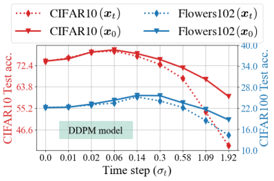
Figure 11: Performance comparison: clean vs. noisy inputs. We use pre-trained DDPM/EDM model on the CIFAR10/CIFAR100 datasets and Flowers-102 [Nilsback and Zisserman, 2008]. The feature probing accuracy is plotted to compare the performance when using clean versus noisy inputs.

Extend $\mathrm{CSNR}$ on feature representations.

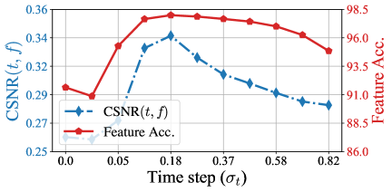
Figure 12: Dynamics of feature probing accuracy and associated $\mathrm{CSNR}$ on MoLRG data Feature probing accuracy is plotted alongside $\mathrm{CSNR}(\hat{f}_{\bm{\theta}},t)$. Probing accuracy is evaluated on the test set, while the empirical $\mathrm{CSNR}$ is computed from the training set. Both exhibit an aligning unimodal pattern.

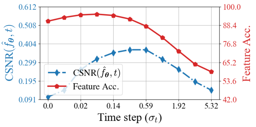
(a) CIFAR10

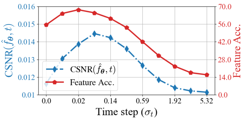
(b) MiniImageNet

Figure 13: Dynamics of feature probing accuracy and associated $\mathrm{CSNR}$ on CIFAR10 and MiniImageNet. Feature probing accuracy is plotted alongside $\mathrm{CSNR}(\hat{f}_{\bm{\theta}},t)$. Probing accuracy is evaluated on the test set, while the empirical $\mathrm{CSNR}$ is computed from the training set. Both exhibit an aligning unimodal pattern.

In the main body of the paper, we define $\mathrm{CSNR}$ with respect to the posterior estimation function. Given that the intermediate representations of diffusion models exhibit near-linear properties [Kwon et al., 2022], we extend the definition of $\mathrm{CSNR}$ to feature extraction functions:

$$\mathrm{CSNR}(t,f_{\bm{\theta}}):=\operatorname{\mathbb{E}}_{k}\left[\frac{\operatorname{\mathbb{E}}_{\bm{x}_{0}}[\|\hat{\bm{U}}_{k}\hat{\bm{U}}_{k}^{T}f_{\bm{\theta}}(\bm{x}_{0},t)\|^{2}\mid k]}{\operatorname{\mathbb{E}}_{\bm{x}_{0}}[\sum_{l\neq k}\|\hat{\bm{U}}_{l}\hat{\bm{U}}_{l}^{T}f_{\bm{\theta}}(\bm{x}_{0},t)\|^{2}\mid k]}\right]$$

Here, $f_{\bm{\theta}}(\cdot,t)$ represents a diffusion feature extraction function that includes all layers up to the feature extraction layer of a diffusion model. The matrix $\hat{\bm{U}}_{k}$ denotes the extracted basis corresponding to the correct class of the features, while $\hat{\bm{U}}_{l}(l\neq k)$ represents the bases of incorrect classes.

We validate this extension of $\mathrm{CSNR}$ as a measure of feature representation quality. Using the same models from Figure˜5 and Figure˜6, we extract intermediate features at each time step and evaluate classification performance on the test set via linear probing. For $\mathrm{CSNR}$ calculation, we compute the basis using features extracted at each time step and subsequently calculate $\mathrm{CSNR}$ for the extracted features, denoted as $\mathrm{CSNR}(\hat{f}_{\bm{\theta}},t)$. The results are presented in Figure˜12 and Figure˜13 for synthetic and real datasets, respectively. As shown in the plots, $\mathrm{CSNR}(f_{\bm{\theta}},t)$ consistently follows a unimodal pattern, mirroring the trend of feature probing performance as the noise scale increases.

Validation of $\hat{\bm{x}}_{\textit{approx}}^{\star}$ approximation in Section˜A.4.2.

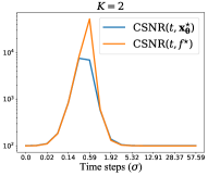
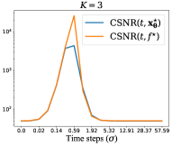
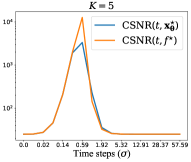
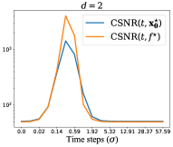
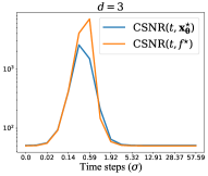
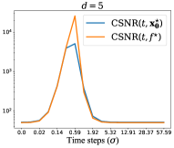
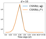
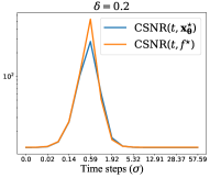
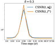
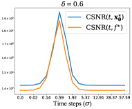
Figure 14: Comparison between $\mathrm{CSNR}$ calculated using the optimal model $\hat{\bm{x}}_{\bm{\theta}}^{\star}$ and the $\mathrm{CSNR}$ calculated with our approximation in Theorem˜1. We generate MoLRG data and calculate $\mathrm{CSNR}$ using both the corresponding optimal posterior function $\hat{\bm{x}}_{\bm{\theta}}^{\star}$ and our approximation $\hat{\bm{x}}_{\textit{approx}}^{\star}$ from Theorem˜1. Default parameters are set as $n=50$, $d=5$, $K=3$, and $\delta=0.1$. In each row, we vary one parameter while keeping the others fixed, comparing the actual and approximated $\mathrm{CSNR}$.

In Theorem˜2, we approximate the optimal posterior estimation function $\hat{\bm{x}}_{\bm{\theta}}^{\star}$ using $\hat{\bm{x}}_{\textit{approx}}^{\star}$ by taking the expectation inside the softmax with respect to $\bm{x}_{0}$. To validate this approximation, we compare the $\mathrm{CSNR}$ calculated from $\hat{\bm{x}}_{\bm{\theta}}^{\star}$ and from $\hat{\bm{x}}_{\textit{approx}}^{\star}$ using the definition in ˜1 and (5) in Section˜A.4.2, respectively. We use a fixed dataset size of $2400$ and set the default parameters to $n=50$, $d=5$, $K=3$, and $\delta=0.1$ to generate MoLRG data. We then vary one parameter at a time while keeping the others constant, and present the computed $\mathrm{CSNR}$ in Figure˜14. As shown, the approximated $\mathrm{CSNR}$ score consistently aligns with the actual score.

Visualization of the MoLRG posterior estimation and $\mathrm{CSNR}$ across noise scales.

In Figure˜5, we show that both the posterior classification accuracy and $\mathrm{CSNR}$ exhibit a unimodal trend for the MoLRG data. To further illustrate this behavior, we provide a visualization of the posterior estimation and $\mathrm{CSNR}$ at different noise scales in Figure˜15. In the plot, each class is represented by a colored straight line, while deviations from these lines correspond to the $\delta$-related noise term. Initially, increasing the noise scale effectively cancels out the $\delta$-related data noise, resulting in a cleaner posterior estimation and improved probing accuracy. However, as the noise continues to increase, the class confidence rate drops, leading to an overlap between classes, which ultimately degrades the feature quality and probing performance.

Figure 15: Visualization of posterior estimation for a clean input, higher $\mathrm{CSNR}$ correspondings to higher classification accuracy. The same MoLRG data is fed into the models; each row represents a different denoising model, and each column corresponds to a different time step with noise scale ($\sigma_{t}$). The teal box indicates the best generation quality and The red box indicates the best representation quality.

Mitigating the performance gap between DAE and diffusion models.

Throughout the empirical results presented in this paper, we consistently observe a performance gap between individual DAEs and diffusion models, especially in low-noise regions. Here, we use a DAE trained on the CIFAR10 dataset with a single noise level $\sigma=0.002$, using the NCSN++ architecture [Karras et al., 2022]. In the default setting, the DAE achieves a test accuracy of $32.3$. We then explore three methods to improve the test performance: (a) adding dropout, as noise regularization and dropout have been effective in preventing autoencoders from learning identity functions [Steck, 2020]; (b) adopting EDM-based preconditioning during training, including input/output scaling, loss weighting, etc.; and (c) multi-level noise training, in which the DAE is trained simultaneously on three noise levels $[0.002,0.012,0.102]$. Each modification is applied independently, and the results are reported in Table˜3. As shown, dropout helps improve performance, but even with a dropout rate of $0.95$, the improvement is minor. EDM-based preconditioning achieves moderate improvement, while multi-level noise training yields the most promising results, demonstrating the benefit of incorporating the diffusion process in DAE training.

Table 3: Improve DAE representation performance at low noise region. A vanilla DAE trained on the CIFAR-10 dataset with a single noise level of $\sigma=0.002$ serves as the baseline. We evaluate the performance improvement of dropout regularization, EDM-based preconditioning, and multi-level noise training ($\sigma=\{0.002,0.012,0.102\}$). Each technique is applied independently to assess its contribution to performance enhancement.

Modifications	Test acc.
Vanilla DAE	$32.3$
+Dropout (0.5)	$35.3$
+Dropout (0.9)	$36.4$
+Dropout (0.95)	$38.1$
+EDM preconditioning	$49.2$
+Multi-level noise training	58.6

A.3 Experimental Details

In this section, we provide technical details for all the experiments in the main body of the paper.

Experimental details for Figure˜1.

• Experimental details for Figure˜1(a). We train diffusion models based on the unified framework proposed by [Karras et al., 2022]. Specifically, we use the DDPM+ network, and use VP configuration for Figure˜1(a). [Karras et al., 2022] has shown equivalence between VP configuration and the traditional DDPM setting, thus we call the models in Figure˜3(a) as DDPM* models. We train two models on CIFAR10 and CIFAR100, respectively. After training, we conduct linear probe on CIFAR10 and CIFAR100. At a specific noise level $\sigma(t)$, we either use clean image $\bm{x}_{0}$ or noisy image $\bm{x}_{t}=\bm{x}_{0}+\bm{n}$ as input to the DDPM* models for extracting features after the ’8x8_block3’ layer. Here, $\bm{n}$ represents random noise and $\bm{n}\sim\mathcal{N}\left(\mathbf{0},\sigma(t)^{2}\mathbf{I}\right)$. We train a logistic regression on features in the train split and report the classification accuracy on the test split of the dataset. We perform the linear probe for each of the following noise levels: [0.002, 0.008, 0.023, 0.060, 0.140, 0.296, 0.585, 1.088, 1.923, 3.257].

• Experimental details for Figure˜1(b). We exactly follow the protocol in [Baranchuk et al., 2022], using the same datasets which are subsets of CelebA [Karras et al., 2018] and FFHQ [Karras et al., 2021], the same training procedure, and the same segmentation networks (MLPs). The only difference is that we use a newer latent diffusion model [Rombach et al., 2022] pretrained on CelebAHQ from Hugging Face and the noise are added to the latent space. For feature extraction we concatenate the feature from the first layer of each resolution in the UNet’s decoder (after upsampling them to the same resolution as the input). We perform segmentation for each of the following noise levels:[0.015, 0.045, 0.079, 0.112, 0.176, 0.342, 0.724, 2.041].

Experimental details for Figure˜3.

We use a pre-trained EDM CIFAR10 model from the official GitHub repository [Karras et al., 2022] and extract 10 sets of posterior estimations corresponding to $\sigma_{t}$ values ranging from 0.002 to 8.401. MLP probing is applied to these posterior estimations to evaluate posterior accuracy, and FID [Heusel et al., 2017] is computed relative to the original CIFAR10 dataset. For the posterior visualizations in the bottom figure, we randomly select a sample and display its posterior estimations according to the same $\sigma_{t}$ schedule.

Experimental details for Figure˜5 and Figure˜15.

For the MoLRG experiments, we train a 3-layer MLP with ReLU activation and a hidden dimension of 1024, following the setup provided in an open-source repository [tanelp, 2022]. The MLP is trained for 200 epochs using DDPM scheduling with $T=500$, employing the Adam optimizer with a learning rate of $5\times 10^{-4}$. For feature extraction, we use the activations of the second layer of the MLP (dimension 1024) as intermediate features for linear probing. For $\mathrm{CSNR}$ computation, we follow the definition in Section˜3.2 since we have access to the ground-truth basis for the MoLRG data, i.e., $\bm{U}_{1},\bm{U}_{2}$, and $\bm{U}_{3}\in\mathbb{R}^{50\times 15}$ . For probing we simply train a linear probe on the posterior and estimations, noting that we take the absolute value of the posterior estimations before feeding them to the probe.

For both panels in Figure˜5, we train our probe the same training set used for diffusion and test on five different MoLRG datasets generated with five different random seeds, reporting the average accuracy and $\mathrm{CSNR}$ at time steps [1, 5, 10, 20, 40, 60, 80, 100, 120, 140, 160, 180, 240, 260, 280]. In Figure˜15, we switch to a 3-class MoLRG with $d=1,n=10,\delta=0.3$ and visualize the posterior estimations at time steps [1, 20, 80, 200, 260] by projecting them onto the union of $\bm{U}_{1},\bm{U}_{2}$, and $\bm{U}_{3}$ (a 3D space), then further projecting onto the 2D plane by a random $3\times 2$ matrix with orthonormal columns. The subtitles of each visualization show the corresponding $\mathrm{CSNR}$ calculated as explained above.

Experimental details for Figure˜6.

We use pre-trained EDM models [Karras et al., 2022] for CIFAR10 and ImageNet, extracting feature representations from the best-performing layer and posterior estimations as the network outputs at each timestep . For the ImageNet model, features are extracted using images and classes from MiniImageNet [Vinyals et al., 2016]. Feature accuracy is evaluated via linear probing, while posterior accuracy is assessed using a two-layer MLP, where posterior estimations pass through a linear layer and ReLU activation before the final linear classifier. The bases for the $\mathrm{CSNR}$ metric on features are computed via singular value decomposition (SVD) on feature representations at each timestep for each class, followed by $\mathrm{CSNR}$ calculation using its definition in Section˜3.2. For posterior estimation, we directly use bases $\bm{U}_{k}$ derived from raw dataset images. In all cases, the first $5$ right singular vectors of each class are used to extract $\bm{U}_{k}$.

Experimental details for Figure˜7.

We train individual DAEs using the DDPM++ network and VP configuration outlined in Karras et al. [2022] at the following noise scales:

$$[0.002,0.008,0.023,0.06,0.14,0.296,0.585,1.088,1.923,3.257].$$

Each model is trained for 500 epochs using the Adam optimizer [Kingma, 2015] with a fixed learning rate of $1\times 10^{-4}$. For the diffusion models, we reuse the model from Figure˜3(d). The sliced Wasserstein distance is computed according to the implementation described in Doan et al. [2024].

Experimental details for Figure˜8 and Figure˜9.

We use the DDPM++ network and VP configuration to train diffusion models[Karras et al., 2022] on the CIFAR10 dataset, using two network configurations: UNet-$64$ and UNet-$128$, by varying the embedding dimension of the UNet. Training dataset sizes range exponentially from $2^{6}$ to $2^{15}$. For each dataset size, both UNet-$64$ and UNet-$128$ are trained on the same subset of the training data. All models are trained with a duration of $50$K images following the EDM training setup. After training, we calculate the generalization score as described in Zhang et al. [2023], using $10$K generated images and the full training subset to compute the score.

Experimental details for Table˜1 and Table˜2

For EDM, we use the official pre-trained checkpoints on ImageNet $64\times 64$ from [Karras et al., 2022], and for DiT, we use the released DiT-XL/2 model pre-trained on ImageNet $256\times 256$ from [Peebles and Xie, 2023]. As a baseline, we include the Hugging Face pre-trained MAE encoder (ViT-B/16) [He et al., 2022].

For diffusion models, features are extracted from the layer and timestep that achieve the highest probing accuracy, following [Xiang et al., 2023]. After feature extraction, we adopt the probing protocol from [Chen et al., 2024b], passing the extracted features through a probe consisting of a BatchNorm1d layer followed by a linear layer. To ensure fair comparisons, all input images are cropped or resized to $224\times 224$, matching the resolution used for MAE training.

For ensembling, we extract features from two additional timesteps on either side of the optimal timestep. Independent probes are trained on these timesteps, yielding five probes in total. At test time, we apply a soft-voting ensemble by averaging the output logits from all five probes for the final prediction. Specifically, let $\bm{W}_{t}\in\mathbb{R}^{K\times d}$ be the linear classifier trained on features from timestep $t$, and let $\bm{h}_{t}\in\mathbb{R}^{d}$ denote the feature representation of a sample at timestep $t$. Considering neighboring timesteps $t-2,t-1,t+1$, and $t+2$, our ensemble prediction is computed as:

$$\bm{\hat{}}{y}=\operatorname*{\text{arg~max}}\left(\frac{1}{5}\sum_{t=t-2}^{t+2}\bm{W}_{t}\bm{h}_{t}\right).$$

We evaluate each method under varying levels of label noise, ranging from $0\%$ to $80\%$, by randomly mislabeling the specified percentage of training labels before applying linear probing. Performance is assessed on both the pre-training dataset and downstream transfer learning tasks. For pre-training evaluation, we use the images and classes from MiniImageNet [Vinyals et al., 2016] to reduce computational cost. For transfer learning, we evaluate on CIFAR100 [Krizhevsky et al., 2009], DTD [Cimpoi et al., 2014], and Flowers102 [Nilsback and Zisserman, 2008].

A.4 Proofs

A.4.1 Proof of ˜1

Proof.

We follow the same proof steps as in [Wang et al., 2024] Lemma $1$ with a change of variable. Let $\bm{c}_{k}=\begin{bmatrix}\bm{a}_{k}\\ \bm{e}_{k}\end{bmatrix}$ and $\widetilde{\bm{U}_{k}}=\begin{bmatrix}\bm{U}_{k}&\delta\bm{U}_{k}^{\perp}\end{bmatrix}$, we first compute

$$p_{t}(\bm{x}|Y=k)$$

$$=\int p_{t}\left(\bm{x}|Y=k,\bm{c}_{k})\mathcal{N}(\bm{c}_{k};\bm{0},\bm{I}_{d+D}\right){\rm d}\bm{c}_{k}$$

$$=\int p_{t}(\bm{x}|\bm{x}_{0}=\widetilde{\bm{U}_{k}}\bm{c}_{k})\mathcal{N}\left(\bm{c}_{k};\bm{0},\bm{I}_{d+D}\right){\rm d}\bm{c}_{k}$$

$$=\int\mathcal{N}(\bm{x};s_{t}\widetilde{\bm{U}_{k}}\bm{c}_{k},\gamma_{t}^{2}\bm{I}_{n})\mathcal{N}\left(\bm{c}_{k};\bm{0},\bm{I}_{d+D}\right){\rm d}\bm{c}_{k}$$

$$=\frac{1}{(2\pi)^{n/2}(2\pi)^{(d+D)/2}\gamma_{t}^{n}}\int\exp\left(-\frac{1}{2\gamma_{t}^{2}}\|\bm{x}-s_{t}\widetilde{\bm{U}_{k}}\bm{c}_{k}\|^{2}\right)\exp\left(-\frac{1}{2}\|\bm{c}_{k}\|^{2}\right){\rm d}\bm{c}_{k}$$

$$=\frac{1}{(2\pi)^{n/2}(2\pi)^{(d+D)/2}\gamma_{t}^{n}}\int\exp\left(-\frac{1}{2\gamma_{t}^{2}}\left(\bm{x}^{T}\bm{x}-2s_{t}\bm{x}^{T}\widetilde{\bm{U}_{k}}\bm{c}_{k}+s_{t}^{2}\bm{c}_{k}^{T}\widetilde{\bm{U}_{k}}^{T}\widetilde{\bm{U}_{k}}\bm{c}_{k}+\gamma_{t}^{2}\bm{c}_{k}^{T}\bm{c}_{k}\right)\right){\rm d}\bm{c}_{k}$$

$$=\frac{1}{(2\pi)^{n/2}\gamma_{t}^{n}}\left(\frac{s_{t}^{2}+\gamma_{t}^{2}}{\gamma_{t}^{2}}\right)^{-d/2}\left(\frac{s_{t}^{2}\delta^{2}+\gamma_{t}^{2}}{\gamma_{t}^{2}}\right)^{-D/2}\exp\left(-\frac{1}{2\gamma_{t}^{2}}\bm{x}^{T}\left(\bm{I}_{n}-\frac{s_{t}^{2}}{s_{t}^{2}+\gamma_{t}^{2}}\bm{U}_{k}\bm{U}_{k}^{T}-\frac{s_{t}^{2}\delta^{2}}{s_{t}^{2}\delta^{2}+\gamma_{t}^{2}}\bm{U}_{k}^{\perp}\bm{U}_{k}^{\perp T}\right)\bm{x}\right)$$

$$\ \int\frac{1}{(2\pi)^{d/2}}\left(\frac{\gamma_{t}^{2}}{s_{t}^{2}+\gamma_{t}^{2}}\right)^{-d/2}\exp\left(-\frac{s_{t}^{2}+\gamma_{t}^{2}}{2\gamma_{t}^{2}}\left\|\bm{a}_{k}-\frac{s_{t}}{s_{t}^{2}+\gamma_{t}^{2}}\bm{U}_{k}^{T}\bm{x}\right\|^{2}\right){\rm d}\bm{a}_{k}$$

$$\ \int\frac{1}{(2\pi)^{D/2}}\left(\frac{\gamma_{t}^{2}}{s_{t}^{2}\delta^{2}+\gamma_{t}^{2}}\right)^{-D/2}\exp\left(-\frac{s_{t}^{2}\delta^{2}+\gamma_{t}^{2}}{2\gamma_{t}^{2}}\left\|\bm{e}_{k}-\frac{s_{t}\delta}{s_{t}^{2}\delta^{2}+\gamma_{t}^{2}}\bm{U}_{k}^{\perp T}\bm{x}\right\|^{2}\right){\rm d}\bm{e}_{k}$$

$$=\frac{1}{(2\pi)^{n/2}}\frac{1}{(s_{t}^{2}+\gamma_{t}^{2})^{d/2}(s_{t}^{2}\delta^{2}+\gamma_{t}^{2})^{D/2}}\exp\left(-\frac{1}{2\gamma_{t}^{2}}\bm{x}^{T}\left(\bm{I}_{n}-\frac{s_{t}^{2}}{s_{t}^{2}+\gamma_{t}^{2}}\bm{U}_{k}\bm{U}_{k}^{T}-\frac{s_{t}^{2}\delta^{2}}{s_{t}^{2}\delta^{2}+\gamma_{t}^{2}}\bm{U}_{k}^{\perp}\bm{U}_{k}^{\perp T}\right)\bm{x}\right)$$

$$=\frac{1}{(2\pi)^{n/2}\det^{1/2}(s_{t}^{2}\bm{U}_{k}\bm{U}_{k}^{T}+s_{t}^{2}\delta^{2}\bm{U}_{k}^{\perp}\bm{U}_{k}^{\perp T}+\gamma_{t}^{2}\bm{I}_{n})}$$

$$\;\;\;\;\;\exp\left(-\frac{1}{2}\bm{x}^{T}\left(s_{t}^{2}\bm{U}_{k}\bm{U}_{k}^{T}+s_{t}^{2}\delta^{2}\bm{U}_{k}^{\perp}\bm{U}_{k}^{\perp T}+\gamma_{t}^{2}\bm{I}_{n}\right)^{-1}\bm{x}\right)$$

$$=\mathcal{N}(\bm{x};\bm{0},s_{t}^{2}\bm{U}_{k}\bm{U}_{k}^{T}+s_{t}^{2}\delta^{2}\bm{U}_{k}^{\perp}\bm{U}_{k}^{\perp T}+\gamma_{t}^{2}\bm{I}_{n}),$$

where we repeatedly apply the pdf of multi-variate Gaussian and the second last equality uses $\det(s_{t}^{2}\bm{U}_{k}\bm{U}_{k}^{T}+s_{t}^{2}\delta^{2}\bm{U}_{k}^{\perp}\bm{U}_{k}^{\perp T}+\gamma_{t}^{2}\bm{I}_{n})=(s_{t}^{2}+\gamma_{t}^{2})^{d}(s_{t}^{2}\delta^{2}+\gamma_{t}^{2})^{D}$ and $(s_{t}^{2}\bm{U}_{k}\bm{U}_{k}^{T}+s_{t}^{2}\delta^{2}\bm{U}_{k}^{\perp}\bm{U}_{k}^{\perp T}+\gamma_{t}^{2}\bm{I}_{n})^{-1}=\left(\bm{I}_{n}-s_{t}^{2}/(s_{t}^{2}+\gamma_{t}^{2})\bm{U}_{k}\bm{U}_{k}^{T}-s_{t}^{2}\delta^{2}/(s_{t}^{2}\delta^{2}+\gamma_{t}^{2})\bm{U}_{k}^{\perp}\bm{U}_{k}^{\perp T}\right)/\gamma_{t}^{2}$ because of the Woodbury matrix inversion lemma. Hence, with $\operatorname{\mathbb{P}}\left(Y=k\right)=\pi_{k}$ for each $k\in[K]$, we have

$$p_{t}(\bm{x}) =\sum_{k=1}^{K}p_{t}(\bm{x}|Y=k)\mathbb{P}(Y=k)=\sum_{k=1}^{K}\pi_{k}\mathcal{N}(\bm{x};\bm{0},s_{t}^{2}\bm{U}_{k}\bm{U}_{k}^{T}+s_{t}^{2}\delta^{2}\bm{U}_{k}^{\perp}\bm{U}_{k}^{\perp T}+\gamma_{t}^{2}\bm{I}_{n}).$$

Now we can compute the score function

$$\nabla\log p_{t}(\bm{x}) =\frac{\nabla p_{t}(\bm{x})}{p_{t}(\bm{x})}=\frac{\begin{multlined}\sum_{k=1}^{K}\pi_{k}\mathcal{N}(\bm{x};\bm{0},s_{t}^{2}\bm{U}_{k}\bm{U}_{k}^{T}+s_{t}^{2}\delta^{2}\bm{U}_{k}^{\perp}\bm{U}_{k}^{\perp T}+\gamma_{t}^{2}\bm{I}_{n})\\ \left(-\frac{1}{\gamma_{t}^{2}}\bm{x}+\frac{s_{t}^{2}}{\gamma_{t}^{2}(s_{t}^{2}+\gamma_{t}^{2})}\bm{U}_{k}\bm{U}_{k}^{T}\bm{x}+\frac{s_{t}^{2}\delta^{2}}{\gamma_{t}^{2}(s_{t}^{2}\delta^{2}+\gamma_{t}^{2})}\bm{U}_{k}^{\perp}\bm{U}_{k}^{\perp T}\bm{x}\right)\end{multlined}\sum_{k=1}^{K}\pi_{k}\mathcal{N}(\bm{x};\bm{0},s_{t}^{2}\bm{U}_{k}\bm{U}_{k}^{T}+s_{t}^{2}\delta^{2}\bm{U}_{k}^{\perp}\bm{U}_{k}^{\perp T}+\gamma_{t}^{2}\bm{I}_{n})\\ \left(-\frac{1}{\gamma_{t}^{2}}\bm{x}+\frac{s_{t}^{2}}{\gamma_{t}^{2}(s_{t}^{2}+\gamma_{t}^{2})}\bm{U}_{k}\bm{U}_{k}^{T}\bm{x}+\frac{s_{t}^{2}\delta^{2}}{\gamma_{t}^{2}(s_{t}^{2}\delta^{2}+\gamma_{t}^{2})}\bm{U}_{k}^{\perp}\bm{U}_{k}^{\perp T}\bm{x}\right)}{\sum_{k=1}^{K}\pi_{k}\mathcal{N}(\bm{x};\bm{0},s_{t}^{2}\bm{U}_{k}\bm{U}_{k}^{T}+s_{t}^{2}\delta^{2}\bm{U}_{k}^{\perp}\bm{U}_{k}^{\perp T}+\gamma_{t}^{2}\bm{I}_{n})}$$

$$=-\frac{1}{\gamma_{t}^{2}}\left(\bm{x}-\frac{\begin{multlined}\sum_{k=1}^{K}\pi_{k}\mathcal{N}(\bm{x};\bm{0},s_{t}^{2}\bm{U}_{k}\bm{U}_{k}^{T}+s_{t}^{2}\delta^{2}\bm{U}_{k}^{\perp}\bm{U}_{k}^{\perp T}+\gamma_{t}^{2}\bm{I}_{n})\\ \left(\frac{s_{t}^{2}}{s_{t}^{2}+\gamma_{t}^{2}}\bm{U}_{k}\bm{U}_{k}^{T}\bm{x})+\frac{s_{t}^{2}\delta^{2}}{s_{t}^{2}\delta^{2}+\gamma_{t}^{2}}\bm{U}_{k}^{\perp}\bm{U}_{k}^{\perp T}\bm{x})\right)\end{multlined}\sum_{k=1}^{K}\pi_{k}\mathcal{N}(\bm{x};\bm{0},s_{t}^{2}\bm{U}_{k}\bm{U}_{k}^{T}+s_{t}^{2}\delta^{2}\bm{U}_{k}^{\perp}\bm{U}_{k}^{\perp T}+\gamma_{t}^{2}\bm{I}_{n})\\ \left(\frac{s_{t}^{2}}{s_{t}^{2}+\gamma_{t}^{2}}\bm{U}_{k}\bm{U}_{k}^{T}\bm{x})+\frac{s_{t}^{2}\delta^{2}}{s_{t}^{2}\delta^{2}+\gamma_{t}^{2}}\bm{U}_{k}^{\perp}\bm{U}_{k}^{\perp T}\bm{x})\right)}{\sum_{k=1}^{K}\pi_{k}\mathcal{N}(\bm{x};\bm{0},s_{t}^{2}\bm{U}_{k}\bm{U}_{k}^{T}+s_{t}^{2}\delta^{2}\bm{U}_{k}^{\perp}\bm{U}_{k}^{\perp T}+\gamma_{t}^{2}\bm{I}_{n})}\right).$$

According to Tweedie’s formula, we have

$$\operatorname{\mathbb{E}}\left[\bm{x}_{0}|\bm{x}_{t}\right] =\frac{\bm{x}_{t}+\gamma_{t}^{2}\nabla\log p_{t}(\bm{x}_{t})}{s_{t}}$$

$$=\frac{s_{t}}{s_{t}^{2}+\gamma_{t}^{2}}\frac{\sum_{k=1}^{K}\pi_{k}\mathcal{N}(\bm{x};\bm{0},s_{t}^{2}\bm{U}_{k}\bm{U}_{k}^{T}+s_{t}^{2}\delta^{2}\bm{U}_{k}^{\perp}\bm{U}_{k}^{\perp T}+\gamma_{t}^{2}\bm{I}_{n})\bm{U}_{k}\bm{U}_{k}^{T}\bm{x}}{\mathcal{N}(\bm{x};\bm{0},s_{t}^{2}\bm{U}_{k}\bm{U}_{k}^{T}+s_{t}^{2}\delta^{2}\bm{U}_{k}^{\perp}\bm{U}_{k}^{\perp T}+\gamma_{t}^{2}\bm{I}_{n})}$$

$$\;\;+\frac{s_{t}\delta^{2}}{s_{t}^{2}\delta^{2}+\gamma_{t}^{2}}\frac{\sum_{k=1}^{K}\pi_{k}\mathcal{N}(\bm{x};\bm{0},s_{t}^{2}\bm{U}_{k}\bm{U}_{k}^{T}+s_{t}^{2}\delta^{2}\bm{U}_{k}^{\perp}\bm{U}_{k}^{\perp T}+\gamma_{t}^{2}\bm{I}_{n})\bm{U}_{k}^{\perp}\bm{U}_{k}^{\perp T}\bm{x}}{\mathcal{N}(\bm{x};\bm{0},s_{t}^{2}\bm{U}_{k}\bm{U}_{k}^{T}+s_{t}^{2}\delta^{2}\bm{U}_{k}^{\perp}\bm{U}_{k}^{\perp T}+\gamma_{t}^{2}\bm{I}_{n})}$$

$$=\dfrac{s_{t}}{s_{t}^{2}+\gamma_{t}^{2}}\frac{\sum_{k=1}^{K}\pi_{k}\exp\left(\phi_{t}\|\bm{U}_{k}^{T}\bm{x}_{t}\|^{2}\right)\exp\left(\psi_{t}\|\bm{U}_{k}^{\perp T}\bm{x}_{t}\|^{2}\right)\bm{U}_{k}\bm{U}_{k}^{T}\bm{x}_{t}}{\sum_{k=1}^{K}\pi_{k}\exp\left(\phi_{t}\|\bm{U}_{k}^{T}\bm{x}_{t}\|^{2}\right)\exp\left(\psi_{t}\|\bm{U}_{k}^{\perp T}\bm{x}_{t}\|^{2}\right)}$$

$$\;\;+\dfrac{s_{t}\delta^{2}}{s_{t}^{2}\delta^{2}+\gamma_{t}^{2}}\frac{\sum_{k=1}^{K}\pi_{k}\exp\left(\phi_{t}\|\bm{U}_{k}^{T}\bm{x}_{t}\|^{2}\right)\exp\left(\psi_{t}\|\bm{U}_{k}^{\perp T}\bm{x}_{t}\|^{2}\right)\bm{U}_{k}^{\perp}\bm{U}_{k}^{\perp T}\bm{x}_{t}}{\sum_{k=1}^{K}\pi_{k}\exp\left(\phi_{t}\|\bm{U}_{k}^{T}\bm{x}_{t}\|^{2}\right)\exp\left(\psi_{t}\|\bm{U}_{k}^{\perp T}\bm{x}_{t}\|^{2}\right)},$$

with $\phi_{t}=s_{t}^{2}/(2\gamma_{t}^{2}(s_{t}^{2}+\gamma_{t}^{2}))$ and $\psi_{t}=s_{t}^{2}\delta^{2}/(2\gamma_{t}^{2}(s_{t}^{2}\delta^{2}+\gamma_{t}^{2}))$. The final equality uses the pdf of multi-variant Gaussian and the matrix inversion lemma discussed earlier.

Now since $\pi_{k}$ is consistent for all $k$ and $s_{t}=1$, we have

$$\operatorname{\mathbb{E}}\left[\bm{x}_{0}|\bm{x}_{t}\right] =\sum_{k=1}^{K}w^{\star}_{k}(\bm{x}_{t})\left(\frac{1}{1+\sigma_{t}^{2}}\bm{U}_{k}\bm{U}_{k}^{T}+\frac{\delta^{2}}{\delta^{2}+\sigma_{t}^{2}}\bm{U}_{k}^{\perp}\bm{U}_{k}^{\perp T}\right)\bm{x}_{t}$$

$$\text{where}\ w^{\star}_{k}(\bm{x}_{t}):=\frac{\exp\left(\frac{1}{2\sigma_{t}^{2}(1+\sigma_{t}^{2})}\|\bm{U}_{k}^{T}\bm{x}_{t}\|^{2}+\frac{\delta^{2}}{2\sigma_{t}^{2}(\delta^{2}+\sigma_{t}^{2})}\|\bm{U}_{k}^{\perp T}\bm{x}_{t}\|^{2}\right)}{\sum_{k=1}^{K}\exp\left(\frac{1}{2\sigma_{t}^{2}(1+\sigma_{t}^{2})}\|\bm{U}_{k}^{T}\bm{x}_{t}\|^{2}+\frac{\delta^{2}}{2\sigma_{t}^{2}(\delta^{2}+\sigma_{t}^{2})}\|\bm{U}_{k}^{\perp T}\bm{x}_{t}\|^{2}\right)}.$$

∎

A.4.2 Proof of Theorem˜1

We first state the formal version of Theorem˜1.

To simplify the calculation of $\mathrm{CSNR}$ as introduced in Section˜3.2 on posterior estimation, which involves the expectation over the softmax term $w^{\star}_{k}$, we approximate $\hat{\bm{x}}_{\bm{\theta}}^{\star}$ as follows:

$$\begin{split}\hat{\bm{x}}_{\textit{approx}}^{\star}(\bm{x},t)&=\sum_{k=1}^{K}\hat{w}_{k}\left(\frac{1}{1+\sigma_{t}^{2}}\bm{U}_{k}\bm{U}_{k}^{T}+\frac{\delta^{2}}{\delta^{2}+\sigma_{t}^{2}}\bm{U}_{k}^{\perp}\bm{U}_{k}^{\perp T}\right)\bm{x},\\ &\text{where}\ \hat{w}_{k}:=\frac{\exp\left(\operatorname{\mathbb{E}}_{\bm{x}_{0}}[g_{k}(\bm{x}_{0},t)]\right)}{\sum_{k=1}^{K}\exp\left(\operatorname{\mathbb{E}}_{\bm{x}_{0}}[g_{k}(\bm{x}_{0},t)]\right)}.\end{split}$$ (5)

In other words, we use $\hat{w}_{k}$ in (5) to approximate $w^{\star}_{k}(\bm{x}_{0})$ in ˜1 by taking expectation inside the softmax with respect to $\bm{x}_{0}$. This allows us to treat $\hat{w}_{k}$ as a constant when calculating $\mathrm{CSNR}$, making the analysis more tractable while maintaining $\operatorname{\mathbb{E}}[\|\bm{U}_{l}\bm{U}_{l}^{T}\hat{\bm{x}}_{\bm{\theta}}^{\star}(\bm{x}_{0},t)\|^{2}]\approx\operatorname{\mathbb{E}}[\|\bm{U}_{l}\bm{U}_{l}^{T}\hat{\bm{x}}_{\textit{approx}}^{\star}(\bm{x}_{0},t)\|^{2}]$ for all $l\in[K]$. We verify the tightness of this approximation at Section˜A.2 (Figure˜14). With this approximation, we state the theorem as follows:

Theorem 2.

Let data $\bm{x}_{0}$ be any arbitrary data point drawn from the MoLRG distribution defined in Assumption 1 and let $k$ denote the true class $\bm{x}_{0}$ belongs to. Then $\mathrm{CSNR}$ introduced in Section˜3.2 depends on the noise level $\sigma_{t}$ in the following form:

$$\mathrm{CSNR}(\hat{\bm{x}}_{\textit{approx}}^{\star},t)=\frac{1}{(K-1)\delta^{2}}\cdot\left(\frac{1+\frac{\sigma_{t}^{2}}{\delta^{2}}h(\hat{w}_{k},\delta)}{1+\frac{\sigma_{t}^{2}}{\delta^{2}}h(\hat{w}_{l},\delta)}\right)^{2}$$ (6)

where $h(w,\delta):=(1-\delta^{2})w+\delta^{2}$. Since $\delta$ is fixed, $h(w,\delta)$ is a monotonically increasing function with respect to $w$. Note that here $\delta$ represents the magnitude of the fixed intrinsic noise in the data where $\sigma_{t}$ denotes the level of additive Gaussian noise introduced during the diffusion training process.

Proof.

Following the definition of $\mathrm{CSNR}$ as defined in Section˜3.2, Lemma˜1 and the fact that $k\sim\text{Mult}(K,\pi_{k})$ with $\pi_{1}=\dots=\pi_{K}=1/K$, we can write

$$\mathrm{CSNR}(\hat{\bm{x}}_{\textit{approx}}^{\star},t) =\frac{\operatorname{\mathbb{E}}_{\bm{x}_{0}}[\|\bm{U}_{k}\bm{U}_{k}^{T}\hat{\bm{x}}_{\textit{approx}}^{\star}(\bm{x}_{0},t)\|^{2}]}{\operatorname{\mathbb{E}}_{\bm{x}_{0}}[\sum_{l\neq k}\|\bm{U}_{l}\bm{U}_{l}^{T}\bm{\hat{}}{\bm{x}}_{\textit{approx}}^{\star}(\bm{x}_{0},t)\|^{2}]}=\frac{\operatorname{\mathbb{E}}_{\bm{x}_{0}}[\|\bm{U}_{k}\bm{U}_{k}^{T}\hat{\bm{x}}_{\textit{approx}}^{\star}(\bm{x}_{0},t)\|^{2}]}{\sum_{l\neq k}\operatorname{\mathbb{E}}_{\bm{x}_{0}}[\|\bm{U}_{l}\bm{U}_{l}^{T}\bm{\hat{}}{\bm{x}}_{\textit{approx}}^{\star}(\bm{x}_{0},t)\|^{2}]}$$

$$=\frac{\left(\frac{\hat{w}_{k}}{1+\sigma_{t}^{2}}+\frac{(K-1)\delta^{2}\hat{w}_{l}}{\delta^{2}+\sigma_{t}^{2}}\right)^{2}d}{(K-1)\left(\frac{\hat{w}_{l}}{1+\sigma_{t}^{2}}+\frac{\delta^{2}(\hat{w}_{k}+(K-2)\hat{w}_{l})}{\delta^{2}+\sigma_{t}^{2}}\right)^{2}\delta^{2}d}$$

$$=\frac{1}{(K-1)\delta^{2}}\cdot\left(\frac{\hat{w}_{k}\delta^{2}+\hat{w}_{k}\sigma_{t}^{2}+(K-1)\delta^{2}\hat{w}_{l}+(K-1)\delta^{2}\hat{w}_{l}\sigma_{t}^{2}}{\hat{w}_{l}\delta^{2}+\hat{w}_{l}\sigma_{t}^{2}+\delta^{2}\hat{w}_{k}+(K-2)\delta^{2}\hat{w}_{l}+\delta^{2}\hat{w}_{k}\sigma_{t}^{2}+(K-2)\delta^{2}\hat{w}_{l}\sigma_{t}^{2}}\right)^{2}$$

$$=\frac{1}{(K-1)\delta^{2}}\cdot\left(\frac{\delta^{2}+\sigma_{t}^{2}\left(\hat{w}_{k}+(K-1)\delta^{2}\hat{w}_{l}\right)}{\delta^{2}+\sigma_{t}^{2}\left(\hat{w}_{l}+\delta^{2}\hat{w}_{k}+(K-2)\delta^{2}\hat{w}_{l}\right)}\right)^{2}$$

$$=\frac{1}{(K-1)\delta^{2}}\cdot\left(\frac{1+\frac{\sigma_{t}^{2}}{\delta^{2}}\left((1-\delta^{2})\hat{w}_{k}+\delta^{2}(\hat{w}_{k}+(K-1)\hat{w}_{l})\right)}{1+\frac{\sigma_{t}^{2}}{\delta^{2}}\left((1-\delta^{2})\hat{w}_{l}+\delta^{2}(\hat{w}_{l}+\hat{w}_{k}+(K-2)\hat{w}_{l})\right)}\right)^{2}$$

$$=\frac{1}{(K-1)\delta^{2}}\cdot\left(\frac{1+\frac{\sigma_{t}^{2}}{\delta^{2}}\left((1-\delta^{2})\hat{w}_{k}+\delta^{2}\right)}{1+\frac{\sigma_{t}^{2}}{\delta^{2}}\left((1-\delta^{2})\hat{w}_{l}+\delta^{2}\right)}\right)^{2}$$

$$=\frac{1}{(K-1)\delta^{2}}\cdot\left(\frac{1+\frac{\sigma_{t}^{2}}{\delta^{2}}h(\hat{w}_{k},\delta)}{1+\frac{\sigma_{t}^{2}}{\delta^{2}}h(\hat{w}_{l},\delta)}\right)^{2}$$

where $h(w,\delta):=(1-\delta^{2})w+\delta^{2}$. ∎

Lemma 1.

With the set up of a K-class MoLRG data distribution as defined in (3), and define the noise space as $\bm{U}_{\perp}=\bigcap_{k=1}^{K}\bm{U}_{k}^{\perp}\in\mathcal{O}^{n\times(n-Kd)}$ (i.e., mutual noise for all classes). Consider the following the function:

$$\hat{\bm{x}}_{\textit{approx}}^{\star}(\bm{x},t) =\sum_{k=1}^{K}\hat{w}_{k}(\bm{x})\left(\frac{1}{1+\sigma_{t}^{2}}\bm{U}_{k}\bm{U}_{k}^{T}+\frac{\delta^{2}}{\delta^{2}+\sigma_{t}^{2}}\bm{U}_{k}^{\perp}\bm{U}_{k}^{\perp T}\right)\bm{x},$$ (7)

$$\text{where}\ \hat{w}_{k}(\bm{x}):=\frac{\exp\left(\operatorname{\mathbb{E}}_{\bm{x}}[g_{k}(\bm{x},t)]\right)}{\sum_{k=1}^{K}\exp\left(\operatorname{\mathbb{E}}_{\bm{x}}[g_{k}(\bm{x},t)]\right)},$$ (8)

$$\text{and}\ g_{k}(\bm{x})=\frac{1}{2\sigma_{t}^{2}(1+\sigma_{t}^{2})}\|\bm{U}_{k}^{T}\bm{x}\|^{2}+\frac{\delta^{2}}{2\sigma_{t}^{2}(\delta^{2}+\sigma_{t}^{2})}\|\bm{U}_{k}^{\perp T}\bm{x}\|^{2}.$$ (9)

I.e., we consider a simplified version of the expected posterior mean as in ˜1 by taking expectation of $g_{k}(\bm{x})$ prior to the softmax operation. Under this setting, for any clean $\bm{x}_{0}$ from class $k$ (i.e., $\bm{x}_{0}=\bm{U}_{k}\bm{a}_{i}+b\bm{U}_{k}^{\perp}\bm{e}_{i}$), we have:

$$\operatorname{\mathbb{E}}_{\bm{x}_{0}}[\|\bm{U}_{k}\bm{U}_{k}^{T}\hat{\bm{x}}_{\textit{approx}}^{\star}(\bm{x}_{0},t)\|^{2}]=\left(\frac{\hat{w}_{k}}{1+\sigma_{t}^{2}}+\frac{(K-1)\delta^{2}\hat{w}_{l}}{\delta^{2}+\sigma_{t}^{2}}\right)^{2}d$$ (10)

$$\operatorname{\mathbb{E}}_{\bm{x}_{0}}[\|\bm{U}_{l}\bm{U}_{l}^{T}\hat{\bm{x}}_{\textit{approx}}^{\star}(\bm{x}_{0},t)\|^{2}]=\left(\frac{\hat{w}_{l}}{1+\sigma_{t}^{2}}+\frac{\delta^{2}(\hat{w}_{k}+(K-2)\hat{w}_{l})}{\delta^{2}+\sigma_{t}^{2}}\right)^{2}\delta^{2}d$$ (11)

$$\operatorname{\mathbb{E}}_{\bm{x}_{0}}[\|\bm{U}_{\perp}\bm{U}_{\perp}^{T}\hat{\bm{x}}_{\textit{approx}}^{\star}(\bm{x}_{0},t)\|^{2}]=\frac{\delta^{6}(n-kd)}{(\delta^{2}+\sigma_{t}^{2})^{2}}$$ (12)

$$\begin{split}\operatorname{\mathbb{E}}[\|\hat{\bm{x}}_{\textit{approx}}^{\star}(\bm{x}_{0},t)\|^{2}]&=\underbrace{\left(\frac{\hat{w}_{k}}{1+\sigma_{t}^{2}}+\frac{(K-1)\delta^{2}\hat{w}_{l}}{\delta^{2}+\sigma_{t}^{2}}\right)^{2}d}_{\operatorname{\mathbb{E}}\|\bm{U}_{k}\bm{U}_{k}^{T}\hat{\bm{x}}_{\textit{approx}}^{\star}(\bm{x}_{0},t)\|^{2}]}\\ &+\underbrace{\left(K-1\right)\left(\frac{\hat{w}_{l}}{1+\sigma_{t}^{2}}+\frac{\delta^{2}(\hat{w}_{k}+(K-2)\hat{w}_{l})}{\delta^{2}+\sigma_{t}^{2}}\right)^{2}\delta^{2}d}_{\operatorname{\mathbb{E}}[\sum_{l\neq k}^{K}\bm{U}_{l}\bm{U}_{l}^{T}\hat{\bm{x}}_{\textit{approx}}^{\star}(\bm{x}_{0},t)\|^{2}]}+\underbrace{\frac{\delta^{6}(n-Kd)}{(\delta^{2}+\sigma_{t}^{2})^{2}}}_{\operatorname{\mathbb{E}}[\|\bm{U}_{\perp}\bm{U}_{\perp}^{T}\hat{\bm{x}}_{\textit{approx}}^{\star}(\bm{x}_{0},t)\|^{2}]}\end{split}$$ (13)

and

$$\begin{split}&\hat{w}_{k}:=\hat{w}_{k}(\bm{x}_{0})=\frac{\exp\left(\frac{d}{2\sigma_{t}^{2}(1+\sigma_{t}^{2})}+\frac{\delta^{4}D}{2\sigma_{t}^{2}(\delta^{2}+\sigma_{t}^{2})}\right)}{\exp\left(\frac{d}{2\sigma_{t}^{2}(1+\sigma_{t}^{2})}+\frac{\delta^{4}D}{2\sigma_{t}^{2}(\delta^{2}+\sigma_{t}^{2})}\right)+\left(K-1\right)\exp\left(\frac{\delta^{2}d}{2\sigma_{t}^{2}(1+\sigma_{t}^{2})}+\frac{\delta^{2}d+\delta^{4}(D-d)}{2\sigma_{t}^{2}(\delta^{2}+\sigma_{t}^{2})}\right)},\\ &\hat{w}_{l}:=\hat{w}_{l}(\bm{x}_{0})=\frac{\exp\left(\frac{\delta^{2}d}{2\sigma_{t}^{2}(1+\sigma_{t}^{2})}+\frac{\delta^{2}d+\delta^{4}(D-d)}{2\sigma_{t}^{2}(\delta^{2}+\sigma_{t}^{2})}\right)}{\exp\left(\frac{d}{2\sigma_{t}^{2}(1+\sigma_{t}^{2})}+\frac{\delta^{4}D}{2\sigma_{t}^{2}(\delta^{2}+\sigma_{t}^{2})}\right)+\left(K-1\right)\exp\left(\frac{\delta^{2}d}{2\sigma_{t}^{2}(1+\sigma_{t}^{2})}+\frac{\delta^{2}d+\delta^{4}(D-d)}{2\sigma_{t}^{2}(\delta^{2}+\sigma_{t}^{2})}\right)}\end{split}$$ (14)

for all class index $l\neq k$.

Proof.

Throughout the proof, we use the following notation for slices of vectors.

$$\bm{e}_{i}[a:b]\;\;\;\;\;\;\text{Slices of vector}\;\bm{e}_{i}\;\text{from}\;a\text{th}\;\text{entry to}\;b\text{th}\;\text{entry.}$$

We begin with the softmax terms. Since each class has its unique disjoint subspace, it suffices to consider $g_{k}(\bm{x}_{0},t)$ and $g_{l}(\bm{x}_{0},t)$ for any $l\neq k$. Let $a_{t}=\frac{1}{2\sigma_{t}^{2}(1+\sigma_{t}^{2})}$ and $c_{t}=\frac{\delta^{2}}{2\sigma_{t}^{2}(\delta^{2}+\sigma_{t}^{2})}$, we have:

$$\operatorname{\mathbb{E}}[g_{k}(\bm{x}_{0},t)] =\operatorname{\mathbb{E}}[a_{t}\|\bm{U}_{k}^{T}\bm{x}_{0}\|^{2}+c_{t}\|\bm{U}_{k}^{\perp T}\bm{x}_{0}\|^{2}]$$

$$=\operatorname{\mathbb{E}}[a_{t}\|\bm{U}_{k}^{T}(\bm{U}_{k}\bm{a}_{i}+b\bm{U}_{k}^{\perp}\bm{e}_{i})\|^{2}]+\operatorname{\mathbb{E}}[c_{t}\|\bm{U}_{k}^{\perp T}(\bm{U}_{k}\bm{a}_{i}+b\bm{U}_{k}^{\perp}\bm{e}_{i})\|^{2}]$$

$$=\operatorname{\mathbb{E}}[a_{t}\|\bm{a}_{i}\|^{2}]+\operatorname{\mathbb{E}}[c_{t}\|b\bm{e}_{i}\|^{2}]$$

$$=a_{t}d+c_{t}\delta^{2}D$$

where the last equality follows from $\bm{a}_{i}\overset{i.i.d.}{\sim}\mathcal{N}(\bm{0},\bm{I}_{d})$ and $\bm{e}_{i}\overset{i.i.d.}{\sim}\mathcal{N}(\bm{0},\bm{I}_{D})$.

Without loss of generality, assume the $j=k+1$, we have:

$$\operatorname{\mathbb{E}}[g_{l}(\bm{x}_{0},t)] =\operatorname{\mathbb{E}}[a_{t}\|\bm{U}_{l}^{T}\bm{x}_{0}\|^{2}+c_{t}\|\bm{U}_{l}^{\perp T}\bm{x}_{0}\|^{2}]$$

$$=\operatorname{\mathbb{E}}[a_{t}\|\bm{U}_{l}^{T}(\bm{U}_{k}\bm{a}_{i}+b\bm{U}_{k}^{\perp}\bm{e}_{i})\|^{2}]+\operatorname{\mathbb{E}}[c_{t}\|\bm{U}_{l}^{\perp T}(\bm{U}_{k}\bm{a}_{i}+b\bm{U}_{k}^{\perp}\bm{e}_{i})\|^{2}]$$

$$=\operatorname{\mathbb{E}}[a_{t}\|b\bm{e}_{i}[1:d]\|^{2}]+\operatorname{\mathbb{E}}\left[c_{t}\Big{\|}\begin{bmatrix}\bm{a}_{i}\\ \bm{0}\in\mathbb{R}^{D-d}\end{bmatrix}+b\begin{bmatrix}\bm{0}\in\mathbb{R}^{d}\\ \bm{e}_{i}[d:D]]\end{bmatrix}\Big{\|}^{2}\right]$$

$$=a_{t}\delta^{2}d+c_{t}(d+\delta^{2}(D-d))$$

Plug $a_{t}$ and $b_{t}$ back with the exponentials, we get $\hat{w}_{k}$ and $\hat{w}_{l}$.

Now we prove (10):

$$\bm{U}_{k}\bm{U}_{k}^{T}\hat{\bm{x}}_{\textit{approx}}^{\star}(\bm{x}_{0},t) =\hat{w}_{k}\bm{U}_{k}\bm{U}_{k}^{T}\left(\frac{1}{1+\sigma_{t}^{2}}\bm{U}_{k}\bm{U}_{k}^{T}+\frac{\delta^{2}}{\delta^{2}+\sigma_{t}^{2}}\bm{U}_{k}^{\perp}\bm{U}_{k}^{\perp T}\right)\bm{x}_{0}$$

$$\;\;\;\;+\sum_{l\neq k}\hat{w}_{l}\bm{U}_{k}\bm{U}_{k}^{T}\left(\frac{1}{1+\sigma_{t}^{2}}\bm{U}_{l}\bm{U}_{l}^{T}+\frac{\delta^{2}}{\delta^{2}+\sigma_{t}^{2}}\bm{U}_{l}^{\perp}\bm{U}_{l}^{\perp T}\right)\bm{x}_{0}$$

$$=\hat{w}_{k}\left(\frac{1}{1+\sigma_{t}^{2}}\bm{U}_{k}\bm{U}_{k}^{T}\bm{x}_{0}\right)+\sum_{l\neq k}\hat{w}_{l}\left(\frac{\delta^{2}}{\delta^{2}+\sigma_{t}^{2}}\bm{U}_{k}\bm{U}_{k}^{T}\bm{x}_{0}\right)$$

$$=\left(\frac{\hat{w}_{k}}{1+\sigma_{t}^{2}}+\frac{\left(K-1\right)\delta^{2}\hat{w}_{l}}{\delta^{2}+\sigma_{t}^{2}}\right)\bm{U}_{k}\bm{U}_{k}^{T}(\bm{U}_{k}\bm{a}_{i}+b\bm{U}_{k}^{\perp}\bm{e}_{i})$$

$$=\left(\frac{\hat{w}_{k}}{1+\sigma_{t}^{2}}+\frac{\left(K-1\right)\delta^{2}\hat{w}_{l}}{\delta^{2}+\sigma_{t}^{2}}\right)\bm{U}_{k}\bm{a}_{i}$$

Since $\bm{U}_{k}\in\mathcal{O}^{n\times d}$:

$$\operatorname{\mathbb{E}}[\|\bm{U}_{k}\bm{U}_{k}^{T}\hat{\bm{x}}_{\textit{approx}}^{\star}(\bm{x}_{0},t)\|^{2}]=\left(\frac{\hat{w}_{k}}{1+\sigma_{t}^{2}}+\frac{\left(K-1\right)\delta^{2}\hat{w}_{l}}{\delta^{2}+\sigma_{t}^{2}}\right)^{2}d$$

and similarly for (11):

$$\bm{U}_{l}\bm{U}_{l}^{T}\hat{\bm{x}}_{\textit{approx}}^{\star}(\bm{x}_{0},t) =\hat{w}_{k}\bm{U}_{l}\bm{U}_{l}^{T}\left(\frac{1}{1+\sigma_{t}^{2}}\bm{U}_{k}\bm{U}_{k}^{T}+\frac{\delta^{2}}{\delta^{2}+\sigma_{t}^{2}}\bm{U}_{k}^{\perp}\bm{U}_{k}^{\perp T}\right)\bm{x}_{0}$$

$$\;\;\;\;+\hat{w}_{l}\bm{U}_{l}\bm{U}_{l}^{T}\left(\frac{1}{1+\sigma_{t}^{2}}\bm{U}_{l}\bm{U}_{l}^{T}+\frac{\delta^{2}}{\delta^{2}+\sigma_{t}^{2}}\bm{U}_{l}^{\perp}\bm{U}_{l}^{\perp T}\right)\bm{x}_{0}$$

$$\;\;\;\;+\sum_{j\neq k,l}\hat{w_{j}}\bm{U}_{l}\bm{U}_{l}^{T}\left(\frac{1}{1+\sigma_{t}^{2}}\bm{U}_{j}\bm{U}_{j}^{T}+\frac{\delta^{2}}{\delta^{2}+\sigma_{t}^{2}}\bm{U}_{j}^{\perp}\bm{U}_{j}^{\perp T}\right)\bm{x}_{0}$$

$$=\hat{w}_{k}\left(\frac{\delta^{2}}{\delta^{2}+\sigma_{t}^{2}}\bm{U}_{l}\bm{U}_{l}^{T}\bm{x}_{0}\right)+\hat{w}_{l}\left(\frac{1}{1+\sigma_{t}^{2}}\bm{U}_{l}\bm{U}_{l}^{T}\bm{x}_{0}\right)+\sum_{j\neq k,l}\hat{w_{j}}\left(\frac{\delta^{2}}{\delta^{2}+\sigma_{t}^{2}}\bm{U}_{l}\bm{U}_{l}^{T}\bm{x}_{0}\right)$$

$$=\left(\frac{\hat{w}_{l}}{1+\sigma_{t}^{2}}+\frac{\delta^{2}(\hat{w}_{k}+(K-2)\hat{w_{j}})}{\delta^{2}+\sigma_{t}^{2}}\right)\bm{U}_{l}\bm{U}_{l}^{T}(\bm{U}_{k}\bm{a}_{i}+b\bm{U}_{k}^{\perp}\bm{e}_{i})$$

$$=\left(\frac{\hat{w}_{l}}{1+\sigma_{t}^{2}}+\frac{\delta^{2}(\hat{w}_{k}+(K-2)\hat{w}_{l})}{\delta^{2}+\sigma_{t}^{2}}\right)b\bm{U}_{l}\bm{e}_{i}[1:d]$$

where the third equality follows since $\hat{w_{j}}=\hat{w}_{l}$ for all $j\neq k,l$. Further, we have:

$$\operatorname{\mathbb{E}}[\|\bm{U}_{l}\bm{U}_{l}^{T}\hat{\bm{x}}_{\textit{approx}}^{\star}(\bm{x}_{0},t)\|^{2}]=\left(\frac{\hat{w}_{l}}{1+\sigma_{t}^{2}}+\frac{\delta^{2}(\hat{w}_{k}+(K-2)\hat{w}_{l})}{\delta^{2}+\sigma_{t}^{2}}\right)^{2}\delta^{2}d$$

Next, we consider (12):

$$\bm{U}_{\perp}\bm{U}_{\perp}^{T}\hat{\bm{x}}_{\textit{approx}}^{\star}(\bm{x}_{0},t) =\hat{w}_{k}\bm{U}_{\perp}\bm{U}_{\perp}^{T}\left(\frac{1}{1+\sigma_{t}^{2}}\bm{U}_{k}\bm{U}_{k}^{T}+\frac{\delta^{2}}{\delta^{2}+\sigma_{t}^{2}}\bm{U}_{k}^{\perp}\bm{U}_{k}^{\perp T}\right)\bm{x}_{0}$$

$$\;\;\;\;+\sum_{l\neq k}\hat{w}_{l}\bm{U}_{\perp}\bm{U}_{\perp}^{T}\left(\frac{1}{1+\sigma_{t}^{2}}\bm{U}_{l}\bm{U}_{l}^{T}+\frac{\delta^{2}}{\delta^{2}+\sigma_{t}^{2}}\bm{U}_{l}^{\perp}\bm{U}_{l}^{\perp T}\right)\bm{x}_{0}$$

$$=\hat{w}_{k}\left(\frac{\delta^{2}}{\delta^{2}+\sigma_{t}^{2}}\bm{U}_{\perp}\bm{U}_{\perp}^{T}\bm{x}_{0}\right)+\sum_{l\neq k}\hat{w}_{l}\left(\frac{\delta^{2}}{\delta^{2}+\sigma_{t}^{2}}\bm{U}_{\perp}\bm{U}_{\perp}^{T}\bm{x}_{0}\right)$$

$$=\frac{\delta^{2}}{\delta^{2}+\sigma_{t}^{2}}\bm{U}_{\perp}\bm{U}_{\perp}^{T}(\bm{U}_{k}\bm{a}_{i}+b\bm{U}_{k}^{\perp}\bm{e}_{i})$$

$$=\frac{\delta^{3}}{\delta^{2}+\sigma_{t}^{2}}\bm{U}_{\perp}\bm{e}_{i}[(K-1)d:D]$$

Hence:

$$\operatorname{\mathbb{E}}[\|\bm{U}_{\perp}\bm{U}_{\perp}^{T}\hat{\bm{x}}_{\textit{approx}}^{\star}(\bm{x}_{0},t)\|^{2}] =\frac{\delta^{6}(n-Kd)}{(\delta^{2}+\sigma_{t}^{2})^{2}}$$

Lastly, we prove (13). Given that the subspaces of all classes and the complement space are both orthonormal and mutually orthogonal, we can write:

$$\operatorname{\mathbb{E}}[\|\hat{\bm{x}}_{\textit{approx}}^{\star}(\bm{x}_{0},t)\|^{2}]=\operatorname{\mathbb{E}}[\|\bm{U}_{k}\bm{U}_{k}^{T}\hat{\bm{x}}_{\textit{approx}}^{\star}(\bm{x}_{0},t)\|^{2}]+\operatorname{\mathbb{E}}[\sum_{l\neq k}\|\bm{U}_{l}\bm{U}_{l}^{T}\hat{\bm{x}}_{\textit{approx}}^{\star}(\bm{x}_{0},t)\|^{2}]+\operatorname{\mathbb{E}}[\|\bm{U}_{\perp}\bm{U}_{\perp}^{T}\hat{\bm{x}}_{\textit{approx}}^{\star}(\bm{x}_{0},t)\|^{2}]$$

Combine terms, we get:

$$\operatorname{\mathbb{E}}[\|\hat{\bm{x}}_{\textit{approx}}^{\star}(\bm{x}_{0},t)\|^{2}] =\left(\frac{\hat{w}_{k}}{1+\sigma_{t}^{2}}+\frac{(K-1)\delta^{2}\hat{w}_{l}}{\delta^{2}+\sigma_{t}^{2}}\right)^{2}d$$

$$+\left(K-1\right)\left(\frac{\hat{w}_{l}}{1+\sigma_{t}^{2}}+\frac{\delta^{2}(\hat{w}_{k}+(K-2)\hat{w}_{l})}{\delta^{2}+\sigma_{t}^{2}}\right)^{2}\delta^{2}d+\frac{\delta^{6}(n-Kd)}{(\delta^{2}+\sigma_{t}^{2})^{2}}.$$

∎

References

- Abstreiter et al. [2021] K. Abstreiter, S. Mittal, S. Bauer, B. Schölkopf, and A. Mehrjou. Diffusion-based representation learning. arXiv preprint arXiv:2105.14257, 2021.
- Achiam et al. [2023] J. Achiam, S. Adler, S. Agarwal, L. Ahmad, I. Akkaya, F. L. Aleman, D. Almeida, J. Altenschmidt, S. Altman, S. Anadkat, et al. Gpt-4 technical report. arXiv preprint arXiv:2303.08774, 2023.
- Alkhouri et al. [2024] I. Alkhouri, S. Liang, R. Wang, Q. Qu, and S. Ravishankar. Diffusion-based adversarial purification for robust deep mri reconstruction. In ICASSP 2024-2024 IEEE International Conference on Acoustics, Speech and Signal Processing (ICASSP), pages 12841–12845. IEEE, 2024.
- Anderson [1982] B. D. Anderson. Reverse-time diffusion equation models. Stochastic Processes and their Applications, 12(3):313–326, 1982.
- Bar-Tal et al. [2024] O. Bar-Tal, H. Chefer, O. Tov, C. Herrmann, R. Paiss, S. Zada, A. Ephrat, J. Hur, G. Liu, A. Raj, et al. Lumiere: A space-time diffusion model for video generation. In SIGGRAPH Asia 2024 Conference Papers, pages 1–11, 2024.
- Baranchuk et al. [2022] D. Baranchuk, A. Voynov, I. Rubachev, V. Khrulkov, and A. Babenko. Label-efficient semantic segmentation with diffusion models. In International Conference on Learning Representations, 2022. URL https://openreview.net/forum?id=SlxSY2UZQT.
- Caron et al. [2021] M. Caron, H. Touvron, I. Misra, H. Jégou, J. Mairal, P. Bojanowski, and A. Joulin. Emerging properties in self-supervised vision transformers. In Proceedings of the IEEE/CVF international conference on computer vision, pages 9650–9660, 2021.
- Chandra and Sharma [2014] B. Chandra and R. K. Sharma. Adaptive noise schedule for denoising autoencoder. In International Conference on Neural Information Processing, 2014.
- Chen et al. [2024a] S. Chen, H. Zhang, M. Guo, Y. Lu, P. Wang, and Q. Qu. Exploring low-dimensional subspace in diffusion models for controllable image editing. In The Thirty-eighth Annual Conference on Neural Information Processing Systems, 2024a. URL https://openreview.net/forum?id=50aOEfb2km.
- Chen et al. [2024b] X. Chen, Z. Liu, S. Xie, and K. He. Deconstructing denoising diffusion models for self-supervised learning. arXiv preprint arXiv:2401.14404, 2024b.
- Choi et al. [2022] J. Choi, J. Lee, C. Shin, S. Kim, H. Kim, and S. Yoon. Perception prioritized training of diffusion models. In Proceedings of the IEEE/CVF Conference on Computer Vision and Pattern Recognition, pages 11472–11481, 2022.
- Chung et al. [2022] H. Chung, B. Sim, D. Ryu, and J. C. Ye. Improving diffusion models for inverse problems using manifold constraints. Advances in Neural Information Processing Systems, 35:25683–25696, 2022.
- Cimpoi et al. [2014] M. Cimpoi, S. Maji, I. Kokkinos, S. Mohamed, , and A. Vedaldi. Describing textures in the wild. In Proceedings of the IEEE Conf. on Computer Vision and Pattern Recognition (CVPR), 2014.
- Deja et al. [2023] K. Deja, T. Trzciński, and J. M. Tomczak. Learning data representations with joint diffusion models. In Joint European Conference on Machine Learning and Knowledge Discovery in Databases, pages 543–559. Springer, 2023.
- Deng et al. [2009] J. Deng, W. Dong, R. Socher, L.-J. Li, K. Li, and L. Fei-Fei. Imagenet: A large-scale hierarchical image database. In 2009 IEEE conference on computer vision and pattern recognition, pages 248–255. Ieee, 2009.
- Doan et al. [2024] A.-D. Doan, B. L. Nguyen, S. Gupta, I. Reid, M. Wagner, and T.-J. Chin. Assessing domain gap for continual domain adaptation in object detection. Computer Vision and Image Understanding, 238:103885, 2024.
- Elhamifar and Vidal [2013] E. Elhamifar and R. Vidal. Sparse subspace clustering: Algorithm, theory, and applications. IEEE transactions on pattern analysis and machine intelligence, 35(11):2765–2781, 2013.
- Fuest et al. [2024] M. Fuest, P. Ma, M. Gui, J. S. Fischer, V. T. Hu, and B. Ommer. Diffusion models and representation learning: A survey. arXiv preprint arXiv:2407.00783, 2024.
- Geras and Sutton [2015] K. Geras and C. Sutton. Scheduled denoising autoencoders. In International Conference on Learning Representations (ICLR) 2015, 2015.
- Gong et al. [2019] S. Gong, V. N. Boddeti, and A. K. Jain. On the intrinsic dimensionality of image representations. In Proceedings of the IEEE/CVF Conference on Computer Vision and Pattern Recognition, pages 3987–3996, 2019.
- Han et al. [2024] A. Han, W. Huang, Y. Cao, and D. Zou. On the feature learning in diffusion models. arXiv preprint arXiv:2412.01021, 2024.
- He et al. [2022] K. He, X. Chen, S. Xie, Y. Li, P. Dollár, and R. Girshick. Masked autoencoders are scalable vision learners. In Proceedings of the IEEE/CVF conference on computer vision and pattern recognition, pages 16000–16009, 2022.
- Heusel et al. [2017] M. Heusel, H. Ramsauer, T. Unterthiner, B. Nessler, and S. Hochreiter. Gans trained by a two time-scale update rule converge to a local nash equilibrium–supplementary material. Advances in Neural Information Processing Systems, 2017.
- Ho et al. [2020] J. Ho, A. Jain, and P. Abbeel. Denoising diffusion probabilistic models. Advances in Neural Information Processing Systems, 33:6840–6851, 2020.
- Ho et al. [2022] J. Ho, W. Chan, C. Saharia, J. Whang, R. Gao, A. Gritsenko, D. P. Kingma, B. Poole, M. Norouzi, D. J. Fleet, et al. Imagen video: High definition video generation with diffusion models. arXiv preprint arXiv:2210.02303, 2022.
- Huang et al. [2024] Z. Huang, Y. Wei, and Y. Chen. Denoising diffusion probabilistic models are optimally adaptive to unknown low dimensionality. arXiv preprint arXiv:2410.18784, 2024.
- Hudson et al. [2024] D. A. Hudson, D. Zoran, M. Malinowski, A. K. Lampinen, A. Jaegle, J. L. McClelland, L. Matthey, F. Hill, and A. Lerchner. Soda: Bottleneck diffusion models for representation learning. In Proceedings of the IEEE/CVF Conference on Computer Vision and Pattern Recognition, pages 23115–23127, 2024.
- Hyvärinen and Dayan [2005] A. Hyvärinen and P. Dayan. Estimation of non-normalized statistical models by score matching. Journal of Machine Learning Research, 6(4), 2005.
- Jing et al. [2022] B. Jing, G. Corso, R. Berlinghieri, and T. Jaakkola. Subspace diffusion generative models. In European Conference on Computer Vision, pages 274–289. Springer, 2022.
- Kadkhodaie et al. [2024] Z. Kadkhodaie, F. Guth, E. P. Simoncelli, and S. Mallat. Generalization in diffusion models arises from geometry-adaptive harmonic representations. In The Twelfth International Conference on Learning Representations, 2024. URL https://openreview.net/forum?id=ANvmVS2Yr0.
- Karras et al. [2018] T. Karras, T. Aila, S. Laine, and J. Lehtinen. Progressive growing of GANs for improved quality, stability, and variation. In International Conference on Learning Representations, 2018. URL https://openreview.net/forum?id=Hk99zCeAb.
- Karras et al. [2021] T. Karras, S. Laine, and T. Aila. A Style-Based Generator Architecture for Generative Adversarial Networks . IEEE Transactions on Pattern Analysis & Machine Intelligence, 43(12):4217–4228, 2021. ISSN 1939-3539. doi: 10.1109/TPAMI.2020.2970919. URL https://doi.ieeecomputersociety.org/10.1109/TPAMI.2020.2970919.
- Karras et al. [2022] T. Karras, M. Aittala, T. Aila, and S. Laine. Elucidating the design space of diffusion-based generative models. In Proc. NeurIPS, 2022.
- Kingma [2013] D. P. Kingma. Auto-encoding variational bayes. arXiv preprint arXiv:1312.6114, 2013.
- Kingma [2015] D. P. Kingma. Adam: A method for stochastic optimization. In International Conference on Learning Representations, 2015.
- Kong et al. [2020] J. Kong, J. Kim, and J. Bae. Hifi-gan: Generative adversarial networks for efficient and high fidelity speech synthesis. Advances in neural information processing systems, 33:17022–17033, 2020.
- Kong et al. [2021] Z. Kong, W. Ping, J. Huang, K. Zhao, and B. Catanzaro. DIFFWAVE: A versatile diffusion model for audio synthesis. In International Conference on Learning Representations, 2021.
- Krizhevsky et al. [2009] A. Krizhevsky, G. Hinton, et al. Learning multiple layers of features from tiny images. 2009.
- Kunin et al. [2019] D. Kunin, J. Bloom, A. Goeva, and C. Seed. Loss landscapes of regularized linear autoencoders. In International conference on machine learning, pages 3560–3569. PMLR, 2019.
- Kwon et al. [2022] M. Kwon, J. Jeong, and Y. Uh. Diffusion models already have a semantic latent space. arXiv preprint arXiv:2210.10960, 2022.
- Lewis et al. [2020] M. Lewis, Y. Liu, N. Goyal, M. Ghazvininejad, A. Mohamed, O. Levy, V. Stoyanov, and L. Zettlemoyer. BART: Denoising sequence-to-sequence pre-training for natural language generation, translation, and comprehension. In Proceedings of the 58th Annual Meeting of the Association for Computational Linguistics, 2020.
- Li et al. [2023] D. Li, H. Ling, A. Kar, D. Acuna, S. W. Kim, K. Kreis, A. Torralba, and S. Fidler. Dreamteacher: Pretraining image backbones with deep generative models. In Proceedings of the IEEE/CVF International Conference on Computer Vision, pages 16698–16708, 2023.
- Li et al. [2024] X. Li, S. M. Kwon, I. R. Alkhouri, S. Ravishanka, and Q. Qu. Decoupled data consistency with diffusion purification for image restoration. arXiv preprint arXiv:2403.06054, 2024.
- Liang et al. [2025] J. Liang, Z. Huang, and Y. Chen. Low-dimensional adaptation of diffusion models: Convergence in total variation. arXiv preprint arXiv:2501.12982, 2025.
- Luo et al. [2024] G. Luo, L. Dunlap, D. H. Park, A. Holynski, and T. Darrell. Diffusion hyperfeatures: Searching through time and space for semantic correspondence. Advances in Neural Information Processing Systems, 36, 2024.
- Mukhopadhyay et al. [2023] S. Mukhopadhyay, M. Gwilliam, V. Agarwal, N. Padmanabhan, A. Swaminathan, S. Hegde, T. Zhou, and A. Shrivastava. Diffusion models beat gans on image classification. arXiv preprint arXiv:2307.08702, 2023.
- Nilsback and Zisserman [2008] M.-E. Nilsback and A. Zisserman. Automated flower classification over a large number of classes. 2008 Sixth Indian Conference on Computer Vision, Graphics & Image Processing, pages 722–729, 2008.
- Peebles and Xie [2023] W. Peebles and S. Xie. Scalable diffusion models with transformers. In Proceedings of the IEEE/CVF International Conference on Computer Vision, pages 4195–4205, 2023.
- Podell et al. [2024] D. Podell, Z. English, K. Lacey, A. Blattmann, T. Dockhorn, J. Müller, J. Penna, and R. Rombach. SDXL: Improving latent diffusion models for high-resolution image synthesis. In The Twelfth International Conference on Learning Representations, 2024.
- Pope et al. [2021] P. Pope, C. Zhu, A. Abdelkader, M. Goldblum, and T. Goldstein. The intrinsic dimension of images and its impact on learning. In International Conference on Learning Representations, 2021. URL https://openreview.net/forum?id=XJk19XzGq2J.
- Preechakul et al. [2022] K. Preechakul, N. Chatthee, S. Wizadwongsa, and S. Suwajanakorn. Diffusion autoencoders: Toward a meaningful and decodable representation. In Proceedings of the IEEE/CVF conference on computer vision and pattern recognition, pages 10619–10629, 2022.
- Pretorius et al. [2018] A. Pretorius, S. Kroon, and H. Kamper. Learning dynamics of linear denoising autoencoders. In International Conference on Machine Learning, pages 4141–4150. PMLR, 2018.
- Radford et al. [2019] A. Radford, J. Wu, R. Child, D. Luan, D. Amodei, and I. Sutskever. Language models are unsupervised multitask learners. 2019.
- Roich et al. [2022] D. Roich, R. Mokady, A. H. Bermano, and D. Cohen-Or. Pivotal tuning for latent-based editing of real images. ACM Transactions on Graphics (TOG), 42(1):1–13, 2022.
- Rombach et al. [2022] R. Rombach, A. Blattmann, D. Lorenz, P. Esser, and B. Ommer. High-resolution image synthesis with latent diffusion models. In Proceedings of the IEEE/CVF Conference on Computer Vision and Pattern Recognition, pages 10684–10695, 2022.
- Ruiz et al. [2023] N. Ruiz, Y. Li, V. Jampani, Y. Pritch, M. Rubinstein, and K. Aberman. Dreambooth: Fine tuning text-to-image diffusion models for subject-driven generation. In Proceedings of the IEEE/CVF conference on computer vision and pattern recognition, pages 22500–22510, 2023.
- Shi et al. [2024] Y. Shi, C. Xue, J. H. Liew, J. Pan, H. Yan, W. Zhang, V. Y. Tan, and S. Bai. Dragdiffusion: Harnessing diffusion models for interactive point-based image editing. In Proceedings of the IEEE/CVF Conference on Computer Vision and Pattern Recognition, pages 8839–8849, 2024.
- Sohl-Dickstein et al. [2015] J. Sohl-Dickstein, E. Weiss, N. Maheswaranathan, and S. Ganguli. Deep unsupervised learning using nonequilibrium thermodynamics. In International Conference on Machine Learning, pages 2256–2265. PMLR, 2015.
- Song et al. [2024] B. Song, S. M. Kwon, Z. Zhang, X. Hu, Q. Qu, and L. Shen. Solving inverse problems with latent diffusion models via hard data consistency. In The Twelfth International Conference on Learning Representations, 2024.
- Song et al. [2021] Y. Song, J. Sohl-Dickstein, D. P. Kingma, A. Kumar, S. Ermon, and B. Poole. Score-based generative modeling through stochastic differential equations. International Conference on Learning Representations, 2021.
- Stanczuk et al. [2022] J. Stanczuk, G. Batzolis, T. Deveney, and C.-B. Schönlieb. Your diffusion model secretly knows the dimension of the data manifold. arXiv preprint arXiv:2212.12611, 2022.
- Steck [2020] H. Steck. Autoencoders that don’t overfit towards the identity. In Neural Information Processing Systems, 2020.
- Stracke et al. [2024] N. Stracke, S. A. Baumann, K. Bauer, F. Fundel, and B. Ommer. Cleandift: Diffusion features without noise. arXiv preprint arXiv:2412.03439, 2024.
- tanelp [2022] tanelp. tiny-diffusion. https://github.com/tanelp/tiny-diffusion, 2022.
- Tang et al. [2023] L. Tang, M. Jia, Q. Wang, C. P. Phoo, and B. Hariharan. Emergent correspondence from image diffusion. Advances in Neural Information Processing Systems, 36:1363–1389, 2023.
- Vincent [2011] P. Vincent. A connection between score matching and denoising autoencoders. Neural computation, 23(7):1661–1674, 2011.
- Vincent et al. [2008] P. Vincent, H. Larochelle, Y. Bengio, and P.-A. Manzagol. Extracting and composing robust features with denoising autoencoders. In International Conference on Machine Learning, 2008.
- Vincent et al. [2010] P. Vincent, H. Larochelle, I. Lajoie, Y. Bengio, and P.-A. Manzagol. Stacked denoising autoencoders: Learning useful representations in a deep network with a local denoising criterion. J. Mach. Learn. Res., 11:3371–3408, 2010.
- Vinyals et al. [2016] O. Vinyals, C. Blundell, T. Lillicrap, D. Wierstra, et al. Matching networks for one shot learning. Advances in neural information processing systems, 29, 2016.
- Wang and Vastola [2023] B. Wang and J. J. Vastola. Diffusion models generate images like painters: an analytical theory of outline first, details later. arXiv preprint arXiv:2303.02490, 2023.
- Wang et al. [2022] P. Wang, H. Liu, A. M.-C. So, and L. Balzano. Convergence and recovery guarantees of the k-subspaces method for subspace clustering. In International Conference on Machine Learning, pages 22884–22918. PMLR, 2022.
- Wang et al. [2024] P. Wang, H. Zhang, Z. Zhang, S. Chen, Y. Ma, and Q. Qu. Diffusion models learn low-dimensional distributions via subspace clustering. arXiv preprint arXiv:2409.02426, 2024.
- Wang et al. [2023] Y. Wang, Y. Schiff, A. Gokaslan, W. Pan, F. Wang, C. De Sa, and V. Kuleshov. Infodiffusion: Representation learning using information maximizing diffusion models. In International Conference on Machine Learning, pages 36336–36354. PMLR, 2023.
- Xiang et al. [2023] W. Xiang, H. Yang, D. Huang, and Y. Wang. Denoising diffusion autoencoders are unified self-supervised learners. In Proceedings of the IEEE/CVF International Conference on Computer Vision, pages 15802–15812, 2023.
- Yang and Wang [2023] X. Yang and X. Wang. Diffusion model as representation learner. In Proceedings of the IEEE/CVF International Conference on Computer Vision, pages 18938–18949, 2023.
- Yu et al. [2024] S. Yu, S. Kwak, H. Jang, J. Jeong, J. Huang, J. Shin, and S. Xie. Representation alignment for generation: Training diffusion transformers is easier than you think. arXiv preprint arXiv:2410.06940, 2024.
- Yue et al. [2024] Z. Yue, J. Wang, Q. Sun, L. Ji, E. I.-C. Chang, and H. Zhang. Exploring diffusion time-steps for unsupervised representation learning. In The Twelfth International Conference on Learning Representations, 2024. URL https://openreview.net/forum?id=bWzxhtl1HP.
- Zhang et al. [2023] H. Zhang, J. Zhou, Y. Lu, M. Guo, P. Wang, L. Shen, and Q. Qu. The emergence of reproducibility and consistency in diffusion models. In Forty-first International Conference on Machine Learning, 2023.
- Zhang et al. [2024] H. Zhang, Y. Lu, I. Alkhouri, S. Ravishankar, D. Song, and Q. Qu. Improving training efficiency of diffusion models via multi-stage framework and tailored multi-decoder architectures. In Conference on Computer Vision and Pattern Recognition 2024, 2024. URL https://openreview.net/forum?id=YtptmpZQOg.
- Zhang and Zhang [2018] Q. Zhang and L. Zhang. Convolutional adaptive denoising autoencoders for hierarchical feature extraction. Frontiers of Computer Science, 12:1140 – 1148, 2018.