Attainability of Two-Point Testing Rates for Finite-Sample
Location Estimation

Abstract

LeCam’s two-point testing method yields perhaps the simplest lower bound for estimating the mean of a distribution: roughly, if it is impossible to well-distinguish a distribution centered at $\mu$ from the same distribution centered at $\mu+\Delta$, then it is impossible to estimate the mean by better than $\Delta/2$. It is setting-dependent whether or not a nearly matching upper bound is attainable. We study the conditions under which the two-point testing lower bound can be attained for univariate mean estimation; both in the setting of location estimation (where the distribution is known up to translation) and adaptive location estimation (unknown distribution). Roughly, we will say an estimate nearly attains the two-point testing lower bound if it incurs error that is at most polylogarithmically larger than the Hellinger modulus of continuity for $\tilde{\Omega}(n)$ samples.

Adaptive location estimation is particularly interesting, as some distributions admit much better guarantees than sub-Gaussian rates (e.g. $\operatorname{Unif}(\mu-1,\mu+1)$ permits error $\Theta(\frac{1}{n})$, while the sub-Gaussian rate is $\Theta(\frac{1}{\sqrt{n}})$), yet it is not obvious whether these rates may be adaptively attained by one unified approach. Our main result designs an algorithm that nearly attains the two-point testing rate for mixtures of symmetric, log-concave distributions with a common mean. Moreover, this algorithm runs in near-linear time and is parameter-free. In contrast, we show the two-point testing rate is not nearly attainable even for symmetric, unimodal distributions.

We complement this with results for location estimation, showing the two-point testing rate is nearly attainable for unimodal distributions, but unattainable for symmetric distributions.

1 Introduction

Estimating the mean of a distribution $D$ from $n$ samples is a well-studied task, both in the setting of location estimation (where $D$ is known up to translation) and adaptive location estimation (where $D$ is unknown). While in some settings the typical estimators such as the sample mean/median are near-optimal (e.g. i.i.d. samples from a Gaussian), in many others there are approaches that may perform much better. A classical example is how for the uniform distribution, $\operatorname{Unif}(\mu-1,\mu+1)$, the sample mean/median will produce an estimate $\hat{\mu}$ with expected error $\mathbb{E}[|\mu-\hat{\mu}|]=\Theta(\frac{1}{\sqrt{n}})$, while the sample midrange (taking the midpoint between the smallest sample and the largest sample) only incurs error $\Theta(\frac{1}{n})$. Such phenomena naturally raise questions regarding how well the mean of any particular distribution can be learned, as well as when there are separations between the non-adaptive and the adaptive settings.

Perhaps the simplest lower bound for this task is given by LeCam’s two-point testing method: if hypothesis testing between $D$ centered at $\mu$ and $D$ centered at $\mu+\Delta$ must fail with constant probability, then any estimator of the mean must incur error at least $\Delta/2$ with constant probability. It is setting-dependent whether or not a nearly matching upper bound is attainable. Our work aims to study the shape-constraints (e.g. symmetric, unimodal, log-concave) under which the two-point testing rate can be attained for the tasks of location estimation and adaptive location estimation. In contrast, distributions have mostly so far been treated on a more case-by-case basis.

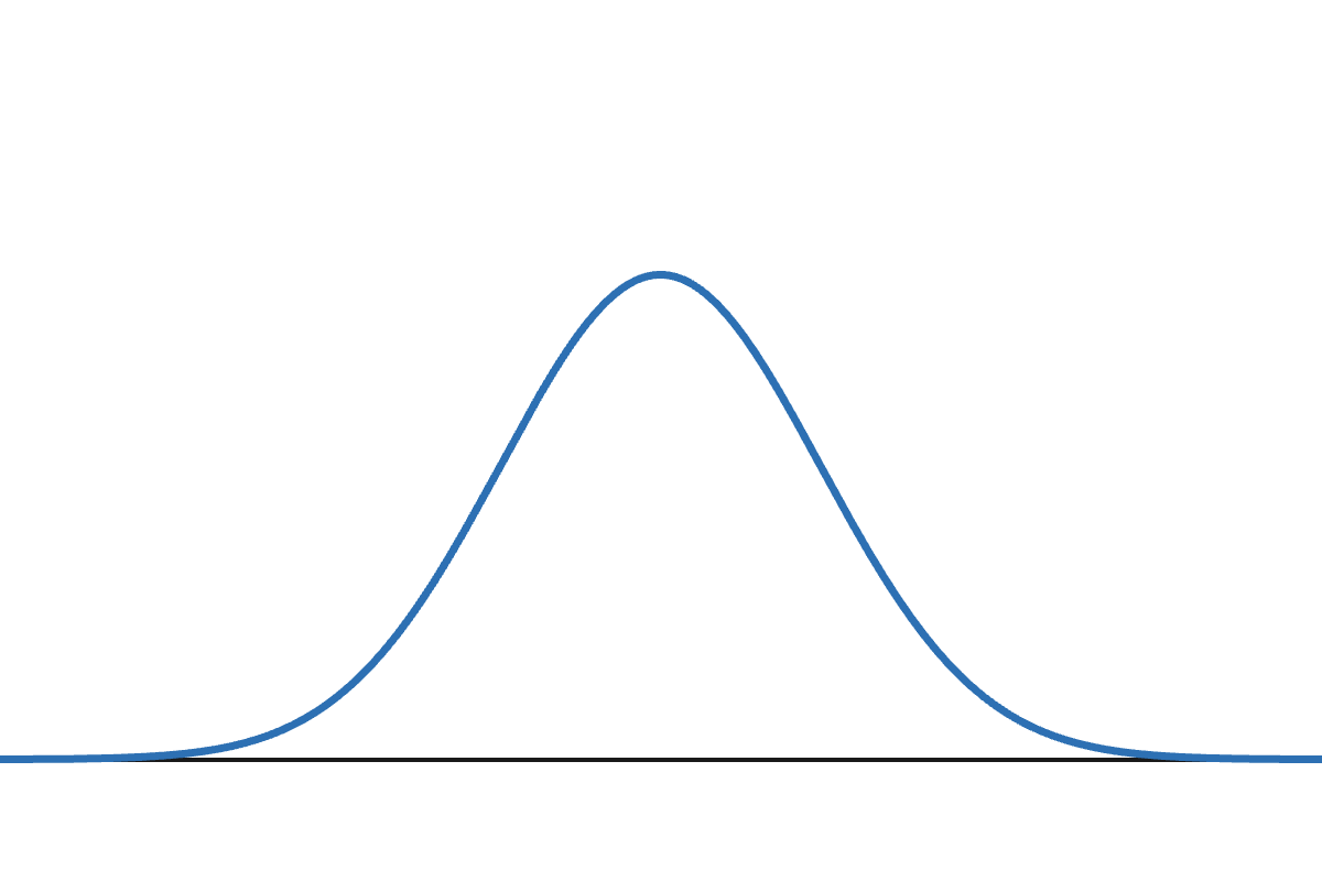
(a) Gaussian

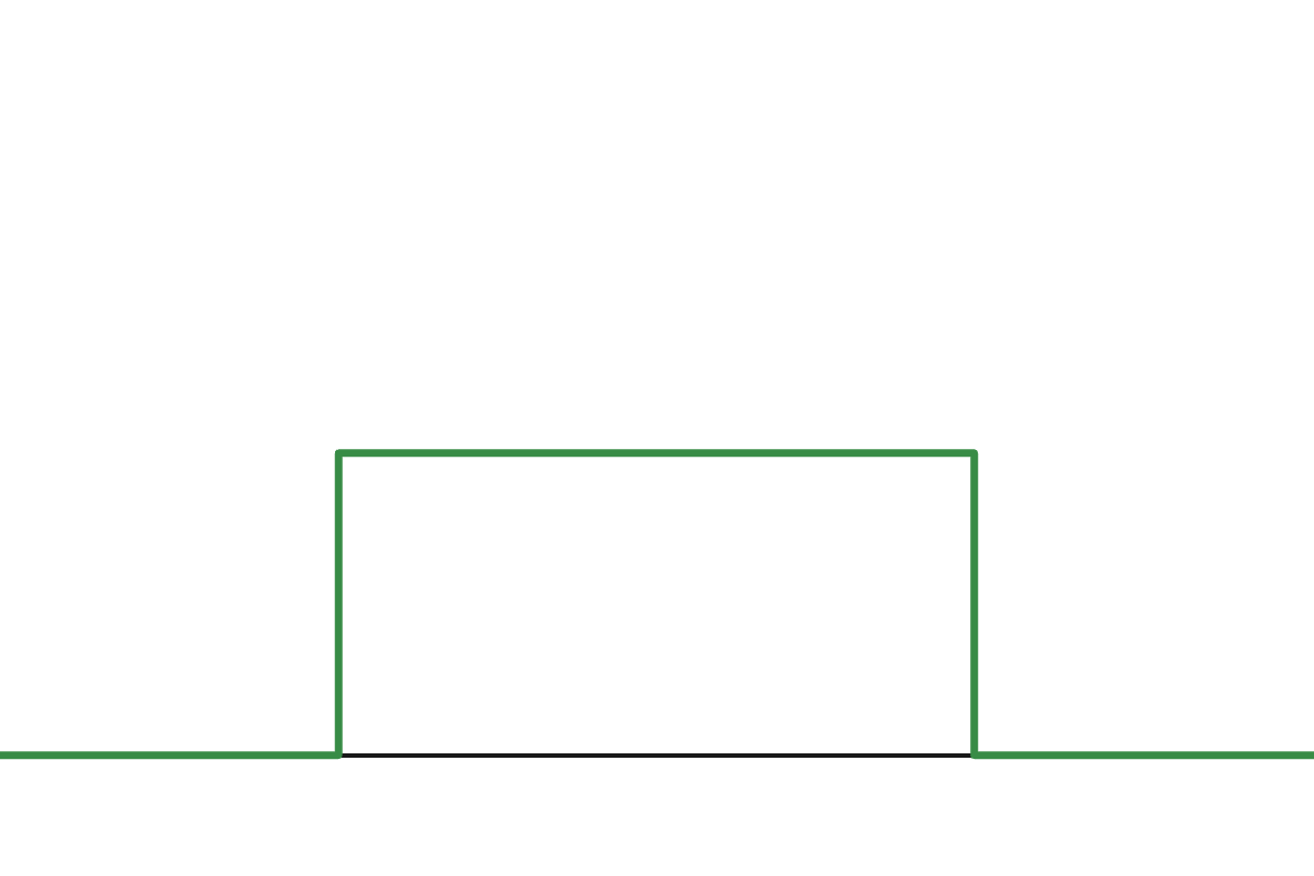
(b) Uniform

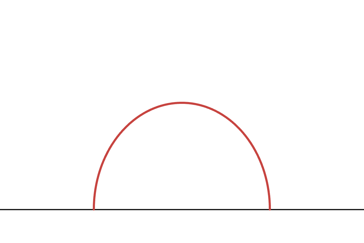
(c) Semicircle: $p(x)\propto\sqrt{1-|x|^{2}}$

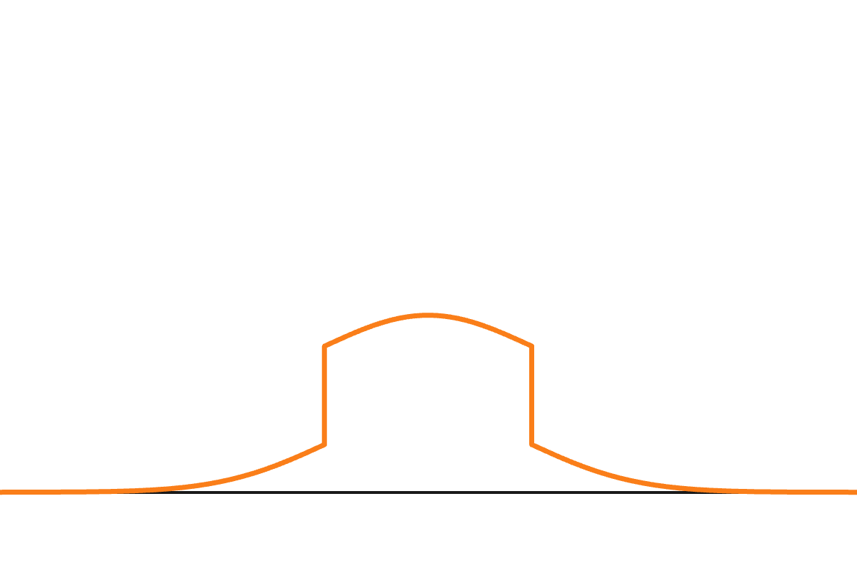
(d) Mixture of a Gaussian and Uniform distribution

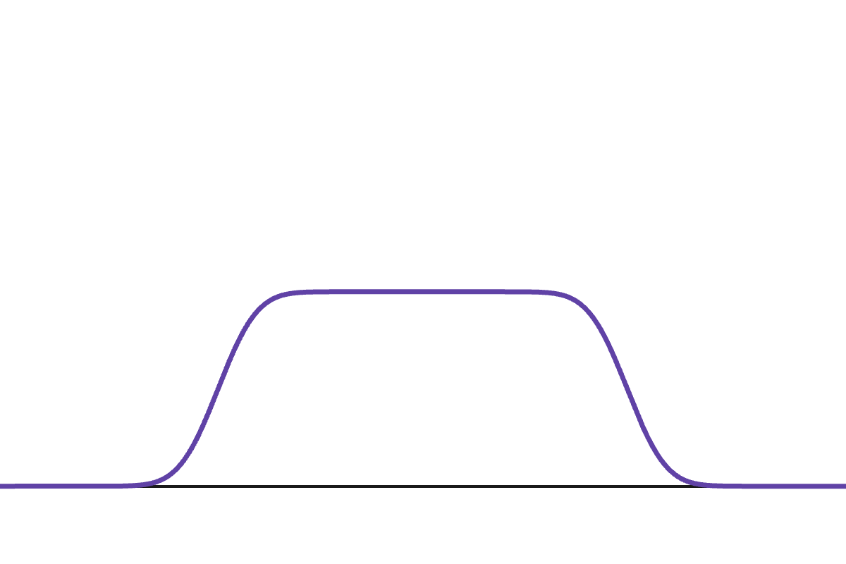
(e) Convolution of a Gaussian and Uniform distribution

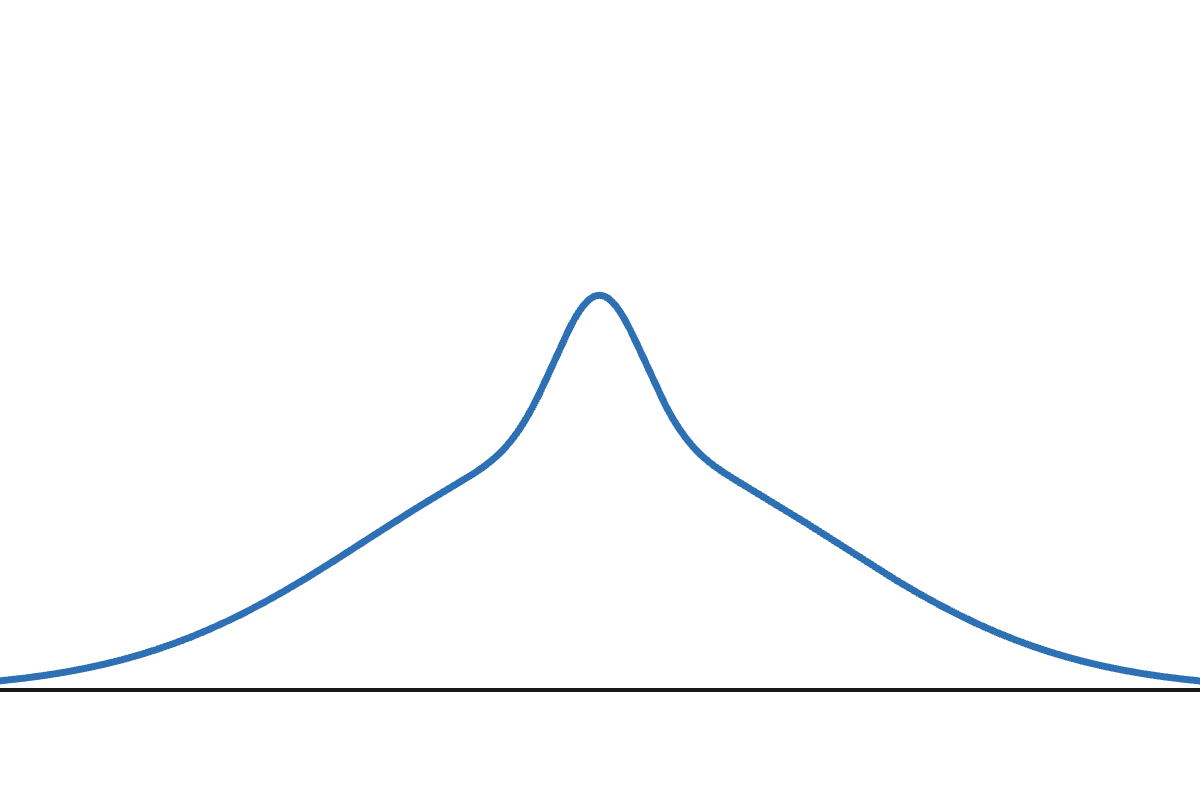
(f) Mixture of two Gaussians with different variances

Figure 1: Examples of symmetric log-concave densities and mixtures of log-concave densities

Examples. Let us showcase some instances that illustrate interesting behaviors for adaptive location estimation.

• For $n$ samples from a Gaussian $N(\mu,\sigma^{2})$, the sample mean/median both incur optimal error of $|\mu-\hat{\mu}|=\Theta(\frac{\sigma}{\sqrt{n}})$.

• For the uniform distribution $\operatorname{Unif}(\mu-1\,\mu+1)$, the sample midrange (the midpoint between the smallest and the largest sample) incurs much better error of $\Theta(\frac{1}{n})$. This phenomenon occurs because there is information in the sharp discontinuity: the sample minimum and maximum concentrate within $\Theta(\frac{1}{n})$ of their expectation; the same phenomena enables $\tilde{O}(n^{-2/3})$ error for the semicircle distribution by the sample midrange.

• For a mixture $\frac{1}{2}N(\mu,1)+\frac{1}{2}\operatorname{Unif}(\mu-1,\mu+1)$ (Fig.˜1(d)), the sample midrange would no longer perform optimally, instead incurring error $\Theta({1}/{\sqrt{\log(n)}})$, yet the MLE would still attain $\Theta(\frac{1}{n})$ (as remarked in [KXZ24]). This begs the question of when knowing the distribution up to translation (so one can, say, use the MLE) changes the rate dramatically. There are many more examples where rates much better than the sub-Gaussian $\Theta(\frac{\sigma}{\sqrt{n}})$ can be attained.

• The convolution of the uniform distribution $\operatorname{Unif}(\mu-1,\mu+1)$ and the Gaussian distribution $N(\mu,n^{-2\alpha})$ (for a constant $\alpha\in(0,1)$; Fig.˜1(e)) is merely a log-concave distribution, yet the earlier approaches are not sharp: the sample median/median incurs error $\tilde{\Theta}(n^{-1/2})$, the sample midrange incurs error $\tilde{\Theta}(n^{-\alpha})$, yet our later results would show the optimal error is $\tilde{\Theta}(n^{-1/2-\alpha/2})$ by more carefully leveraging information from the tails. This sharper rate is not obviously attainable from the guarantees of known prior work.

• Mixtures of Gaussians with a common mean (even a two-component mixture $w_{1}N(\mu,\sigma_{1})+(1-w_{1})N(\mu,\sigma_{2})$ is non-trivial, Fig.˜1(f)) demonstrate interesting behavior, studied as entangled mean estimation or heteroskedastic mean estimation, where works [CDKL14, LY20, YL20, PJL22, DLLZ23, CV24] analyzed a collection of algorithms (median, shorth, modal, iterative trimming, and balance finding estimators) and resolved that the optimal rate entails a phase transition [LY20, CV24].

The examples we presented were all solved by a collection of different estimators, and it is natural to wonder whether a unified approach can adaptively recover near-optimal rates for many distributions. Our main result will design a new algorithm that nearly attains the two-point testing lower bound for all these examples.

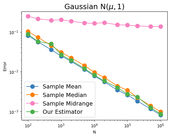
(a)

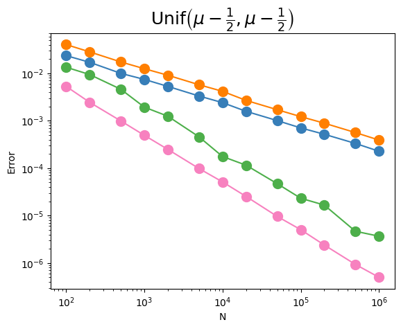
(b)

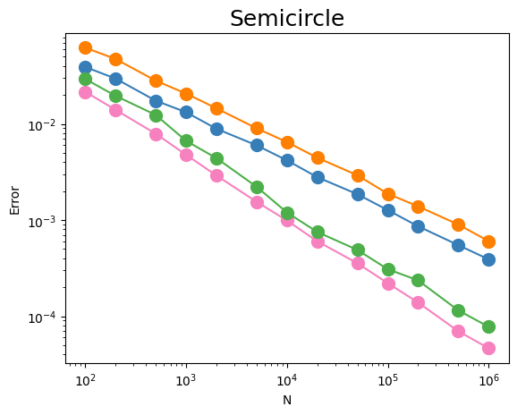
(c)

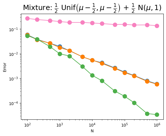
(d)

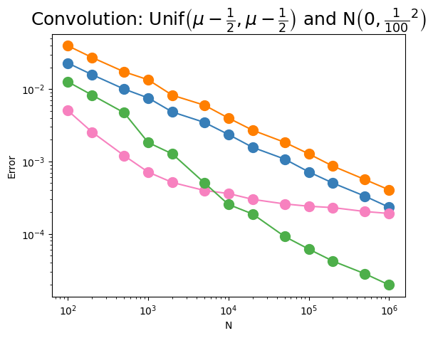
(e)

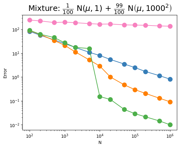
(f)

Figure 2: Performance of our estimator (Algorithm˜2) for corresponding distributions in Fig.˜1.

Simulations. We examine performance of our estimator on these examples in Fig.˜2, where each point is the average of $500$ tests. Running a short Python implementation of our estimator on $N=10^{6}$ samples took approximately $40$ seconds on a laptop. We interpret our estimator in Figs.˜2(a), 2(b), 2(c) and 2(d) as behaving similarly to the optimal rates: $\tilde{\Theta}(\frac{1}{\sqrt{n}})$ (Fig.˜2(a)), $\tilde{\Theta}(\frac{1}{n})$ (Fig.˜2(b)), $\tilde{\Theta}(\frac{1}{n^{2/3}})$ (Fig.˜2(c)), and $\tilde{\Theta}(\frac{1}{n})$ (Fig.˜2(d)). Lagging behind by a multiplicative factor, as in Fig.˜2(b), is not too surprising as our algorithm and analysis are loose up to polylogarithmic factors. In Fig.˜2(e), we observe how when $N$ is small relative to the standard deviation of the Gaussian convolution then behavior is similar to the uniform distribution, for larger $N$ there is information in the tail not leveraged by the other estimators, and for $N$ even larger than our simulation then we expect sample median/mean to improve beyond sample midrange and close the gap with our estimator (recall our earlier discussion of Fig.˜1(e)). Finally, in Fig.˜2(f), we observe a sharp improvement in performance when $N$ is large enough that our estimator is able to detect the mixture component with smaller weight and standard deviation. Collectively, these simulations give some insight into how we adaptively attain sharper guarantees for many distributions with one estimator.

Hellinger modulus of continuity. We now provide background to introduce the Hellinger modulus of continuity which will characterize the two-point testing rate. The Hellinger distance is a distance metric on probability distributions:

Definition 1.1 (Hellinger distance).

If $P,Q$ are distributions over the same probability space $\Omega$ with densities $p$ and $q$, then the squared Hellinger distance between $P$ and $Q$ is

$$\mathsf{d_{h}^{2}}(P,Q)=\frac{1}{2}\int_{\Omega}\left(\sqrt{p(x)}-\sqrt{q(x)}\right)^{2}$$

Throughout this paper, we may also directly reference the Hellinger distance between probability densities. The Hellinger distance may be related to the total variation distance:

Fact 1.2 (e.g. [LCY00] page 44).

$$\mathsf{d_{h}^{2}}(P,Q)\leq\mathsf{d_{TV}}(P,Q)\leq\sqrt{2\mathsf{d_{h}^{2}}(P,Q)}$$

The Hellinger distance tensorizes, which makes it ideal for studying the sample complexity of hypothesis testing.

Fact 1.3 (Tensorization of Hellinger distance; e.g. [LCY00] page 45).

Suppose $P,Q$ are distributions over the same probability space $\Omega$, and let $P^{\otimes n}$ and $Q^{\otimes n}$ denote the distribution of $n$ i.i.d. samples from $P$ and $Q$ respectively. Then

$$\mathsf{d_{h}^{2}}(P^{\otimes n},Q^{\otimes n})=1-\left(1-\mathsf{d_{h}^{2}}(P,Q)\right)^{n}.$$

In particular, as a corollary of Facts˜1.2 and 1.3, the Hellinger distance is ideal for measuring the sample complexity of hypothesis testing between two distributions. If $P,Q$ are distributions over the same probability space, then

$$\mathsf{d_{TV}}(P^{\otimes n},Q^{\otimes n})\geq\left(1-e^{-n\cdot\mathsf{d_{h}^{2}}(P,Q)}\right),$$ (1)

so that once $n\sim\frac{1}{\mathsf{d_{h}^{2}}(P,Q)}$, $n$ samples distinguish between $P$ and $Q$ with at least constant probability. The second inequality in Fact˜1.2 shows that if $n\ll\frac{1}{\mathsf{d_{h}^{2}}(P,Q)}$, hypothesis testing between $P$ and $Q$ with fewer than $n$ samples is information-theoretically impossible except with vanishing probability.

Since the squared Hellinger distance $\mathsf{d_{h}^{2}}(P,Q)$ informs the sample complexity of hypothesis testing between $P$ and $Q$, Donoho and Liu [DL87] introduced the Hellinger modulus of continuity that yields often-sharp two-point testing lower bounds. The Hellinger modulus is defined for a functional $T$ and class $\mathbf{F}$ as

$$\omega(\varepsilon)\triangleq\sup\{|T(F_{1})-T(F_{0})|:\mathsf{d_{h}^{2}}(F_{1},F_{0})\leq\varepsilon,F_{i}\in\mathbf{F}\}.$$

For estimating the mean of a distribution $D$, the Hellinger modulus can be instantiated as

$$\omega_{D}(\varepsilon)\triangleq\sup\{|\mu_{1}-\mu_{2}|:\mathsf{d_{h}^{2}}(D_{\mu_{1}},D_{\mu_{2}})\leq\varepsilon,\,\,\mu_{1},\mu_{2}\in\mathbb{R}\},$$

where $D_{\mu}$ denotes the distribution $D$ centered at $\mu$. Given our earlier background, we see that $\omega_{D}(\frac{1}{n})$ informs some two-point testing style lower bound, since $D_{\mu_{1}}$ and $D_{\mu_{2}}$ will only be distinguishable with constant probability. As immediately explored by Donoho and Liu [DL87, DL91a, DL91b], it is often possible to nearly attain the Hellinger modulus in statistical estimation tasks. For example, they show in [DL91a] the Hellinger modulus rate is asymptomatically attainable if $\mathbf{F}$ is convex, $T$ is linear, and $\omega$ is Hölderian; this style of result is recently furthered in [PW19]. In our setting $T$ is linear, but the main obstacle in employing techniques from such works is that our class $\mathbf{F}$ is not convex. Observe how convex combinations of translations of $D$ are not necessarily a translation of $D$. Similarly, shape-constraints do not form a convex set either; convex combinations of translations of symmetric distributions need not be symmetric.

We will study the shape-constraints on $D$ under which it is possible to attain error $|\mu-\hat{\mu}|\leq\operatorname{polylog}(n)\cdot\omega_{D}(\frac{\operatorname{polylog}(n)}{n})$ (our formal statement of results will add dependence on a failure probability $\delta$). This roughly corresponds to error that is polylogarithmically larger than the two-point testing bound for $\frac{n}{\operatorname{polylog}(n)}$ samples.

1.1 Preliminaries

A probability density $p$ is a $k$-mixture if $p(x)=\sum_{i=1}^{k}w_{i}\cdot p_{i}(x)$, where $w_{i}\geq 0$, $\sum_{i=1}^{k}w_{i}=1$, and each $p_{i}$ is a density. It is a $k$-mixture of log-concave distributions if each $p_{i}$ is log-concave. It is a centered/symmetric mixture if all mixture components are symmetric around a common point. We denote $p_{\Delta}$ to be the density $p$ shifted to recenter at $\Delta$, meaning $p_{\Delta}(x)\triangleq p(x-\Delta)$.

1.2 Our Contributions

We present positive and negative results on the attainability of the two-point testing rate, both in the settings of location estimation and adaptive location estimation. We begin with our most interesting finding: the positive result for adaptive location estimation. We follow with our three complementary results that elucidate the landscape of these tasks more broadly.

Attainability for adaptive location estimation. For mixtures of $k$ symmetric log-concave distributions with the same center, we show that the two-point testing rate is nearly attainable:

Theorem 1.4.

Suppose $p$ is a probability density that is a centered/symmetric mixture of $k$ log-concave distributions. There exists some universal constant $C_{\operatorname{dist}}\geq 1$, where if

$$\Delta^{*}\triangleq\omega_{p}\left(C_{\operatorname{dist}}\cdot\frac{k}{n}\cdot\log(2n/\delta)\cdot\log^{2}(2n)\right)$$

then with probability $1-\delta$ the output $\hat{\mu}$ of Algorithm˜2 will satisfy $|\mu-\hat{\mu}|\leq\Delta^{*}/2$. Moreover, Algorithm˜2 always runs in $O(n\log(n)\log(\log(n)))$ time.

Brief intuition. Here is an informal outline of an algorithm that guides our ideas:

1. Consider a possible estimate $\hat{\mu}$ of the true mean $\mu$.

2. Test if there is an interval that reveals the true distribution is not symmetric around $\hat{\mu}$. Precisely, check if there exists an $0\leq a<b$ where the number of samples within $[\hat{\mu}-b,\hat{\mu}-a]$ is noticeably different from the number within $[\hat{\mu}+a,\hat{\mu}+b]$.

3. For any $\hat{\mu}$ that passes this test, hope it is a good estimate of $\mu$.

Nothing is immediately clear about the performance of this algorithm. First, it is not obviously efficient to consider all values of $\hat{\mu},a,b$, but we will delay this concern. Notably, it is not clear how good of an estimate $\hat{\mu}$ must be if it passes these interval tests. For arbitrary symmetric distributions, a $\hat{\mu}$ passing interval tests can indeed be a poor estimate. Surprisingly, we show that for mixtures of log-concave distributions, $\hat{\mu}$ is close (in terms of the Hellinger modulus) to $\mu$ with high probability.

We observe that performance of our informal algorithm boils down to the following key question: if $p$ and a translation of $p$ have large Hellinger distance, must there be an interval of the domain where their expected number of samples are noticeably different? This is not true for general $p$, but we will show it holds for $p$ satisfying our assumptions.

Trying to answer this question, we draw connections to [BNOP21, PJL23] who show how the Hellinger distance between any two distributions can be approximately preserved by a channel $T$ that outputs an indicator of a threshold of the likelihood ratio: i.e. the indicator of $p(x)/q(x)\geq\tau$ for a well-chosen threshold parameter $\tau\geq 0$. Roughly, if $P$ and $Q$ are easy to distinguish from $n$ samples, then $T(P)$ and $T(Q)$ are easy to distinguish from $\tilde{O}(n)$ samples. From their results, it becomes clear that our key question is essentially resolved if the appropriate likelihood threshold channel can be simulated by an indicator of an interval of the domain (we call this an interval statistic). Later, we show that it is also sufficient to approximately simulate the channel.

In the simpler case of $k=1$, a simple calculation reveals that any likelihood threshold channel is exactly simulated by an interval statistic. This is not true for $k>1$, but with non-trivial analysis involving piecewise-approximations of the densities and likelihood ratios, we are able to show that it is still possible to approximate the channel sufficiently well with an interval statistic.

Eventually, we further refine our approach to permit a near-linear time algorithm that still aligns with the intuition of the informal algorithm we discussed. This gives an efficient algorithm (with no tuning parameters) that we evaluated in Fig.˜2 on our examples of Fig.˜1.

Unattainability for adaptive location estimation. We show that if the distribution is only promised to be unimodal and symmetric, then such a rate is unattainable:

Theorem 1.5.

There exists a universal constant $0<C<1$ such that for any $n$ larger than a sufficiently large constant, and $\nu\geq 1$, then for every estimator $\hat{\theta}$ there is a unimodal and symmetric distribution where $\hat{\theta}$ incurs much larger error than the two-point testing rate with constant probability:

$$\min_{\hat{\theta}}\max_{\textrm{unimodal and symmetric $D$,}\,\mu\in\mathbb{R}}\operatorname{{Pr}}_{X\sim D(x-\mu)^{\otimes n},\hat{\theta}}\left[|\hat{\theta}(X)-\mu|\geq\nu\cdot\omega_{D}\left(\frac{C}{\nu\cdot n^{9/10}\sqrt{\log(n)}}\right)\right]\geq\Omega(1)$$

Note that the statement has randomness over $\hat{\theta}$ to account for non-deterministic estimators.

Notably, the exponent for $n$ is $\frac{9}{10}$ instead of 1. Observe that if we invoke this theorem with $\nu=\log(n)^{c}$ for any constant $c$, we rule out the possibility of a positive guarantee of the form $\operatorname{polylog}(n)\cdot\omega_{D}(\tfrac{\operatorname{polylog}(n)}{n})$ since $n^{1/10}>\log^{c}(n)$ for sufficiently large $n$.

Brief intuition. In the proof of our positive result Theorem˜1.4, we crucially leveraged that thresholds of the likelihood ratio of log-concave mixtures and their translations could be well-approximated by interval statistics. For our hard instance, we hope to use a distribution where the likelihood ratio with its translation is large in regions that are very spaced apart, so interval statistics are less helpful because any large interval must contain large fractions of the domain that contain minimal information. Moreover, if we consider a family of such distributions with different spacings, then we expect it will be impossible to find where the likelihood ratio is large. We will show there is no estimator that attains two-point testing rates for all distributions in this family.

More concretely, we consider a step distribution, which is a unimodal and symmetric distribution that resembles a collection of steps. Comparing this distribution with a slight translation in Fig.˜3, we see that the likelihood ratio is unequal to $1$ in regions that are spaced apart. We carefully study a family of step distributions with different step widths, and show this mixture family is indistinguishable from a triangle distribution (which has a worse two-point testing rate).

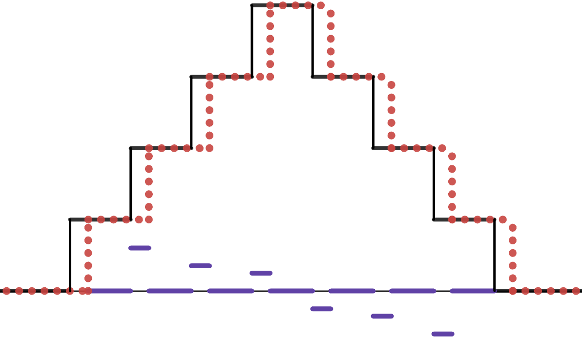
Figure 3: Step distribution (black, solid), a slight translation (red, dotted), and the logarithm of their likelihood ratio (purple, solid). Observe the likelihood ratio is unequal to $1$ in disjoint regions.

Attainability for location estimation. On the other hand, we show the two-point testing rate is attainable for location estimation even when the distribution is only promised to be unimodal:

Theorem 1.6.

Suppose $p$ is a unimodal probability density with mode $p(0)$, $\sqrt{n}\geq 6\log(2/\delta)$, and $\delta\in(0,\frac{1}{2})$. There exists some universal constant $C_{\operatorname{dist}}\geq 1$, where if

$$\Delta^{*}\triangleq\omega_{p}\left(C_{\operatorname{dist}}\cdot\frac{\log(n/\delta)}{n}\right)$$

then with probability $1-\delta$, the output $\hat{\mu}$ of our algorithm will satisfy $|\mu-\hat{\mu}|\leq 4\Delta^{*}$.

We remark that the condition of $\sqrt{n}\geq 6\log(2/\delta)$ is semi-arbitrary, but our proof does need at least some bound on $\delta$ in relation to $n$.

Brief intuition. While the work of [GLPV24] shows that a variant of the MLE attains a form of minimax optimality for this task, it is still not obvious how to directly analyze whether their algorithm attains the two-point testing rate for this task. Thus, we present and analyze a simple approach that attains this guarantee.

For our approach, we use the first $n/2$ samples as candidates for our estimate $\hat{\mu}$. We prove that with high probability, one of these samples $X_{i}$ will satisfy that $\mathsf{d_{h}^{2}}(p_{\mu},p_{X_{i}})\leq O(1)\cdot\frac{\log(1/\delta)}{n}$. Our hope is to perform likelihood tests between pairs of candidate estimates on batches of samples, and then use the results of these tests to choose a candidate. Unfortunately, it is not immediately clear that likelihood tests with $p_{X_{i}}$ will perform well, since although $\mathsf{d_{h}^{2}}(p_{\mu},p_{X_{i}})$ is small, $X_{i}$ is still not exactly $\mu$. The main observation we use is that if we purposefully ‘‘underpower’’ the likelihood tests, using batches of size at most $O(\frac{n}{\log(n/\delta)})$, then since it is impossible to well-distinguish between $p_{\mu}$ and $p_{X_{i}}$ from batches of this size, $p_{X_{i}}$ must perform well on likelihood tests.

We remark that this approach should be fairly straightforward to extend to mixtures of a bounded number of unimodal distributions (not necessarily with the same center) if desired. For our purposes, we primarily desired to show this contrast with the corresponding negative result for unimodal distributions in adaptive location estimation.

Unattainability for location estimation. Finally, we show that if the distribution is only promised to be symmetric, then such a rate is unattainable:

Theorem 1.7.

For any positive integer $n$ and positive value $\nu$, there exists a distribution $D_{n,\nu}$ that is symmetric around $0$, and for every estimator $\hat{\theta}(X)$, there exists a centering $\mu$ where $\hat{\theta}$ incurs large error with constant probability:

$$\min_{\hat{\theta}}\max_{\mu}\operatorname{{Pr}}_{X\sim D_{n,\nu}(x-\mu)^{\otimes n},\hat{\theta}}\left[|\hat{\theta}(X)-\mu|\geq\nu\cdot\omega_{D_{n,\nu}}\left(\frac{1}{10}\right)\right]\geq\frac{1}{4}$$

Note that the statement has randomness over $\hat{\theta}$ to account for non-deterministic estimators.

This indicates that location estimation does not get much easier from symmetry alone, as the lower bound is quite strong: by setting $\nu$ as desired, the error gets arbitrarily worse than $\omega_{D}(\tfrac{1}{10})$, which is already much worse than the $\omega_{D}(\tfrac{1}{n})$ standard for two-point testing. The constants in our theorem statement are semi-arbitrary, but adding more variables to our theorem does not seem more insightful in our primary goal of showing that the two-point testing rate is not even nearly attainable under just an assumption of symmetry.

Brief intuition. Our analysis considers a family of distributions and uses the probabilistic method to conclude that at least one distribution satisfies desired technical properties which enable a type of packing lower bound. Our family of distributions will essentially be uniform distributions $\operatorname{Unif}(\mu-1,\mu+1)$ with a random half of regions of their support missing. The family is slightly modified to enforce symmetry constraints. From the details of our construction, these modified distributions should not actually be much easier to estimate than by using the sample midrange for error $\Theta(\frac{1}{n})$, but the two-point testing lower bound will deceptively look much more favorable.

1.3 Related Work

Asymptotic setting. Location estimation and adaptive location estimation have been more extensively studied in the asymptotic settings: where the distribution $D$ is fixed and then we analyze the performance of estimators as $n\rightarrow\infty$. For location estimation, it is known that the Fisher information rate is attainable: the MLE asymptotically approaches $N(\mu,\tfrac{1}{n\mathcal{I}})$, where $\mathcal{I}$ is the Fisher information of $D$ (e.g. see Chapter 7 of [VdV00]). For adaptive location estimation, many works have studied estimation under the assumption that $D$ is symmetric (e.g. [S⁺56, VE70, Sto75, Sac75, Ber78, DGT06]). Stone [Sto75] showed that the Fisher information rate is asymptotically attainable if $D$ is symmetric. More recently, Laha [Lah19] showed that tuning parameters may be avoided for adaptive location estimation of symmetric distributions if $D$ is also log-concave.

For distributions with infinite Fisher information (e.g. $\operatorname{Unif}(\mu-1,\mu+1)$, non-smooth distributions), it is perhaps sharper to consider a result of LeCam [LeC73] who showed the Hellinger distance two-point testing rate is attainable given conditions related to the covering number of the family under the Hellinger metric.

Finite-sample setting. In this setting, we focus on how well the location may be estimated for a particular $D$ and $n$. The work of [GLPV24] showed that for location estimation, variants of the MLE attained minimax optimal guarantees for any $D$ and $n$, yet it does not necessarily reveal what the optimal rate is. The works of [GLPV22] and [GLP23] study location estimation and adaptive location estimation, respectively, and show how estimators similar to [Sto75] are able to attain the smoothed Fisher information rate, which is the Fisher information of $D$ convolved with $N(0,r^{2})$ (where $r$ is a smoothing parameter that depends on $n$, and they require $D$ is symmetric for adaptive location estimation). For some distributions, this is sufficient to attain guarantees with optimal constant factors. Unfortunately, for other distributions, the smoothing parameter $r$ may be sufficiently large such that too much information is lost. For example, their error guarantees for $\operatorname{Unif}(\mu-1,\mu+1)$ are polynomially worse than $\Theta(\frac{1}{n})$.

The balance finding algorithm of [CV24] for heteroskedastic mean estimation inspires our estimator. The algorithm looks for an estimate $\hat{\mu}$ that exhibits a particular kind of balance, where for parameters $w$ and $\Delta$, the number of samples within $w$ to the left of $\hat{\mu}$ and $w$ to the right of $\hat{\mu}$ are approximately balanced, yet there is strong imbalance for $\hat{\mu}\pm\Delta$. In this way, balance finding also leverages interval statistics to inform its estimator. While the balance finding algorithm attains desired guarantees for the distributions in Figs.˜1(a) and 1(f), it incurs polynomially-suboptimal errors for Figs.˜1(b), 1(c), 1(d) and 1(e). Sweep-line techniques similarly enable near-linear time.

The work of [KXZ24] focuses on adaptive location estimation with the goal of minimizing the $L_{\gamma}$ loss for $\gamma\geq 2$, where $\gamma$ is chosen data-dependently (the guarantees are a mix of asymptotic and finite-sample). Their approach is sufficient to enable sharp rates for distributions such as $\tilde{O}(\frac{1}{n})$ for $\operatorname{Unif}(\mu-1,\mu+1)$ and $\tilde{O}(n^{-2/3})$ for the semicircle distribution. Their results also extend to the regression setting. In their discussion, they remark how this approach is unable to leverage discontinuities in the interior of the support, such as in Fig.˜1(d), which our results will encompass.

Additional related work. For examples such as Fig.˜1(d), much of the difficulty of adaptive location estimation boils down to determining where the discontinuity in the density occurs. In this sense, it is natural that techniques will be shared with the richly-studied task of density estimation. Focusing on log-concave distributions, it is recently known that the log-concave MLE learns the density within optimal Hellinger distance up to logarithmic factors (for any number of dimensions) [HW16, KS16, KDR19]. Most relevant to our work are the techniques of [CDSS14], who (among other results) optimally learn mixtures of log-concave distributions in total variation distance up to logarithmic factors. Their techniques analyze estimates where the number of samples empirically within collections of intervals roughly match the expected number of samples for the estimate. Their analysis uses piecewise-polynomial approximations of log-concave distributions. Later, our work will design an algorithm that also verifies whether indicators of intervals match what is expected given shape-constraints, whose analysis also uses piecewise approximations of log-concave distributions (and a slightly finer notion of matching). This line of prior work is crucially leveraging the notion of $\mathcal{A}_{k}$ distance, roughly defined as the total variation distance witnessed by the union of $k$ disjoint intervals (also studied, for example, by [DL01, DKN14, DKN15, DKN17, DKP19, DKL23]). Our work will later focus instead on the Hellinger distance witnessed by the union of $k$ disjoint intervals.

An interesting recent line of work focuses on getting optimal constant-factor dependence on the sub-Gaussian rate (e.g. [Cat12, LV22b, LV22a, GHP24]). In contrast, our work focuses on shape-constrained distributions where we may perform polynomially better than the sub-Gaussian rate (but incur logarithmic-factors of lossiness in our analysis).

For some recent examples (among many) to showcase the influence of the modulus of continuity perspective: [CL15] introduces a local modulus of continuity as a benchmark for estimating convex functions, [DR24] uses the local modulus of continuity (instead with total variation distance) for locally private estimation, and [FKQR21] presents an analog of the modulus of continuity for interactive learning.

2 Adaptive Location Estimation for Log-Concave Mixtures

In this section, we will provide an algorithm for estimating the mean of mixtures of log-concave distributions, with a guarantee in terms of the Hellinger modulus of the distribution. We begin with recalling an informal outline of an algorithm that guides our ideas:

1. Consider a possible estimate $\hat{\mu}$ of the true mean $\mu$.

2. Test if there is an interval that reveals the true distribution is not symmetric around $\hat{\mu}$. Precisely, check if there exists an $0\leq a<b$ where the number of samples within $[\hat{\mu}-b,\hat{\mu}-a]$ is noticeably different from the number within $[\hat{\mu}+a,\hat{\mu}+b]$.

3. For any $\hat{\mu}$ that passes this test, hope it is a good estimate of $\mu$.

Nothing is immediately clear about the performance of this algorithm. First, it is not obviously efficient to consider all values of $\hat{\mu},a,b$, but we will delay this concern. Notably, it is not clear how good of an estimate $\hat{\mu}$ must be if it passes these interval tests. For arbitrary symmetric distributions, a $\hat{\mu}$ passing interval tests can indeed be a poor estimate. Surprisingly, we will show that for mixtures of log-concave distributions, $\hat{\mu}$ will be close (in terms of the Hellinger modulus) to $\mu$ with high probability:

See 1.4

We now roughly outline our proof structure. Our goal is to show that there exists a failing interval test if $\hat{\mu}$ is poor enough such that $\mathsf{d_{h}^{2}}(p_{\mu},p_{\hat{\mu}})$ is large. Roughly, we will later show that this occurs if whenever $\mathsf{d_{h}^{2}}(p_{\mu},p_{\hat{\mu}})$ is large, there exists some interval that witnesses the distance: the expected number of samples inside this interval is noticeably different for $p_{\mu}$ and $p_{\hat{\mu}}$. We focus on showing this witnessing property first, and then focus on the algorithmic aspects later.

First, in Section˜2.1, we discuss the results of [BNOP21, PJL23] that show how the Hellinger distance between any two distributions can be approximately preserved by a channel that outputs an indicator of a threshold of the likelihood ratio: i.e. the indicator of $p(x)/q(x)\geq\tau$ for a well-chosen threshold parameter $\tau\geq 0$. We then observe how a channel that approximates the optimal thresholding channel still approximately preserves the Hellinger distance between the two distributions. Second, in Section˜2.2, we prove how any likelihood thresholding channel between a log-concave mixture and its translation can be approximated by an interval statistic. This proof relies on a careful approximation of the distribution and likelihood ratio by piecewise-constant functions. Finally, we have shown our desired witnessing property. In Section˜2.3, we combine these tools to show how they imply that any sufficiently bad estimate $\hat{\mu}$ will fail some interval test with high probability. We further refine the structure of these interval tests to permit a near-linear time algorithm that still aligns with the intuition of the informal algorithm we discussed.

2.1 Near-Optimality of Approximate Likelihood Threshold Channels

Consider the task of distinguishing between two distributions $p$ and $q$ from samples. It is classically known that the sample complexity of this task is $\Theta(\frac{1}{H^{2}(p,q)})$ by looking at the product of the likelihood ratio for all samples. Interestingly, [BNOP21] and [PJL23] show that the sample complexity only increases logarithmically if we merely look at statistics of the indicator of a threshold on the likelihood ratio. We will focus on the form of the result given by [PJL23] for convenience, but the result of either paper would yield the tool that is crucial for our work. More concretely, consider the class of thresholds on the likelihood ratio:

Definition 2.1.

$\mathcal{T}^{\operatorname{thresh}}\triangleq\{\mathbbm{1}_{p(x)/q(x)\geq\tau}(x):\tau\geq 0\}$

Then, [PJL23] show there exists a $\textbf{T*}\in\mathcal{T}^{\operatorname{thresh}}$ where $H^{2}(\textbf{T*}p,\textbf{T*}q)\approx H^{2}(p,q)$. We state a special-case of one of their results as follows:

Theorem 2.2 (Corollary 3.4 of [PJL23]; preservation of Hellinger distance).

For any $p,q\in\Delta_{k}$, there exists a $\textbf{T*}\in\mathcal{T}^{\operatorname{thresh}}$ such that the following holds:

$$1\leq\frac{\mathsf{d_{h}^{2}}(p,q)}{\mathsf{d_{h}^{2}}(\textbf{T*}p,\textbf{T*}q)}\leq 1800\min\{k,k^{\prime}\},$$ (2)

where $k^{\prime}=\log(4/\mathsf{d_{h}^{2}}(p,q))$.

We remark on some properties of this result. Note that properties 2-4 simultaneously hold for $p,q$ or after exchanging $p,q$:

Remark 2.3.

1. The proof of Theorem˜2.2 also holds for continuous distributions $p,q$ if we replace the dependence on $\min\{k,k^{\prime}\}$ with just $k^{\prime}$.

2. The proof also implies a stronger bound that $\frac{\mathsf{d_{h}^{2}}(p,q)}{\mathsf{d_{h}^{2}}(\textbf{T*}p,\textbf{T*}q)}\leq\frac{\mathsf{d_{h}^{2}}(p,q)}{\left(\sqrt{\operatorname{{Pr}}_{x\sim p}[\textbf{T*}(x)=1]}-\sqrt{\operatorname{{Pr}}_{x\sim q}[\textbf{T*}(x)=1]}\right)^{2}}\leq 1800\min\{k,k^{\prime}\}$.

3. T* thresholds with $1+\tau^{*}$ for $\tau^{*}\geq 0$ and it holds that $\tau^{*}\geq\sqrt{\frac{\mathsf{d_{h}^{2}}(p,q)}{104\log(4/\mathsf{d_{h}^{2}}(p,q))}}$.

4. T* thresholds with $1+\tau^{*}$ for $\tau^{*}\geq 0$ and it holds that $\operatorname{{Pr}}_{x\sim p}[\textbf{T*}(x)=1]\geq\frac{\mathsf{d_{h}^{2}}(p,q)}{1800\log(4/\mathsf{d_{h}^{2}}(p,q))}$.

Proof.

(1) holds immediately by replacing all notation in their original proof with the corresponding notation for continuous distributions.

(2) holds immediately from their proof as well.

(3) holds from the following observations about their proof (see their Section 3.2 for reference). In their “Case 1”, observe that $\tau^{*}=1$. In their “Case 2”, we use more details in their proof. In terms of their notation (their $\delta$ is our $\tau^{*}$), note that they choose a threshold of $1+\delta$ such that:

$$\delta^{2}$$

$$\geq\delta^{2}\operatorname{{Pr}}[Y\geq\delta^{2}]$$

$$\geq\frac{\mathbb{E}[Y]}{13\cdot(1+\log(1/\mathbb{E}[Y]))}$$

Using their inequality that $$\mathbb{E}[Y]\geq\mathsf{d_{h}^{2}}(p,q)/4$$:

$$\geq\frac{\mathsf{d_{h}^{2}}(p,q)}{52\cdot(1+\log(4/\mathsf{d_{h}^{2}}(p,q)))}$$

$$\geq\frac{\mathsf{d_{h}^{2}}(p,q)}{104\log(4/\mathsf{d_{h}^{2}}(p,q))}$$

As their $\delta$ is our $\tau^{*}$, this implies $\tau^{*}\geq\sqrt{\frac{\mathsf{d_{h}^{2}}(p,q)}{104\log(4/\mathsf{d_{h}^{2}}(p,q))}}$.

(4) holds simply by:

$$\operatorname{{Pr}}_{x\sim p}[\textbf{T*}(x)=1]$$

$$\geq\mathsf{d_{TV}}(\textbf{T*}p,\textbf{T*}q)$$

$$\geq\mathsf{d_{h}^{2}}(\textbf{T*}p,\textbf{T*}q)$$

Using the result of Theorem˜2.2:

$$\geq\frac{\mathsf{d_{h}^{2}}(p,q)}{1800\log(4/\mathsf{d_{h}^{2}}(p,q))}$$

∎

For our work, we hope to leverage a channel T’ (not necessarily a proper thresholding function) that approximates T*, and conclude that T’ similarly preserves Hellinger distance like T*.

Theorem 2.4 (Modified Corollary 3.4 of [PJL23]; preservation of Hellinger distance for approximating thresholds).

For any continuous distributions $p,q$, let $\textbf{T*}\in\mathcal{T}^{\operatorname{thresh}}$ be the threshold yielded by Theorem˜2.2. Without loss of generality, suppose T* thresholds by $1+\tau^{*}$ for $\tau^{*}\geq 0$ (swap $p$ and $q$ otherwise). Then, consider a channel T’ an $(\alpha,\beta)$-approximation if it satisfies:

1. $\textbf{T'}(x)=1$ only if $p(x)/q(x)\geq 1+\alpha\cdot\tau^{*}$ for $0<\alpha\leq 1$.

2. $\operatorname{{Pr}}_{x\sim p}[\textbf{T'}(x)=1]\geq\beta\cdot\operatorname{{Pr}}_{x\sim p}[\textbf{T*}(x)=1]$ for $0<\beta\leq 1$.

For any such $(\alpha,\beta)$-approximation T’, the following holds:

$$1\leq\frac{\mathsf{d_{h}^{2}}(p,q)}{\mathsf{d_{h}^{2}}(\textbf{T'}p,\textbf{T'}q)}\leq\frac{\mathsf{d_{h}^{2}}(p,q)}{\left(\sqrt{\operatorname{{Pr}}_{x\sim p}[\textbf{T'}(x)=1]}-\sqrt{\operatorname{{Pr}}_{x\sim q}[\textbf{T'}(x)=1]}\right)^{2}}\leq\frac{3744k^{\prime}}{\alpha^{2}\beta},$$ (3)

where $k^{\prime}=\log(4/\mathsf{d_{h}^{2}}(p,q))$.

Proof.

The first part of the inequality follows from data-processing inequality, as remarked in [PJL23]. The second part of the inequality follows by definition of Hellinger distance. For the remaining portion, we merely state adjustments for the proof of [PJL23] to include the necessary terms with $\alpha,\beta$.

“Case 1” of [PJL23]. Analogous to their notation (but for continuous distributions), let $A_{2,\infty}$ be the subset of the domain where $p(x)/q(x)\geq 2$. Then, let $p^{\prime}\triangleq\operatorname{{Pr}}_{x\sim p}[x\in A_{2,\infty}]$. As they argue, then $\mathsf{d_{h}^{2}}(p,q)\leq 4p^{\prime}$. We now compute:

$$\left(\sqrt{\operatorname{{Pr}}_{x\sim p}[\textbf{T'}(x)=1]}-\sqrt{\operatorname{{Pr}}_{x\sim q}[\textbf{T'}(x)=1]}\right)^{2}$$

$$\geq\left(\sqrt{\operatorname{{Pr}}_{x\sim p}[\textbf{T'}(x)=1]}-\sqrt{\frac{1}{1+\alpha\cdot\delta}\operatorname{{Pr}}_{x\sim p}[\textbf{T'}(x)=1]}\right)^{2}$$

Recall for this case, $$\delta=1$$:

$$=\left(1-\sqrt{\frac{1}{1+\alpha}}\right)^{2}\cdot\operatorname{{Pr}}_{x\sim p}[\textbf{T'}(x)=1]$$

$$\geq\left(1-\sqrt{\frac{1}{1+\alpha}}\right)^{2}\cdot\beta\cdot\operatorname{{Pr}}_{x\sim p}[\textbf{T*}(x)=1]$$

Observe that $$\operatorname{{Pr}}_{x\sim p}[\textbf{T*}(x)=1]=p^{\prime} p^{\prime}\geq\mathsf{d_{h}^{2}}(p,q)/4$$ and use :

$$\geq\left(1-\sqrt{\frac{1}{1+\alpha}}\right)^{2}\cdot\beta\cdot\frac{\mathsf{d_{h}^{2}}(p,q)}{4}$$

$$\geq\left(1-\sqrt{1-\frac{\alpha}{2}}\right)^{2}\cdot\beta\cdot\frac{\mathsf{d_{h}^{2}}(p,q)}{4}$$

$$\geq\left(\frac{\alpha}{4}\right)^{2}\cdot\beta\cdot\frac{\mathsf{d_{h}^{2}}(p,q)}{4}$$

$$=\alpha^{2}\cdot\beta\cdot\frac{\mathsf{d_{h}^{2}}(p,q)}{64}$$

$$\implies\frac{\mathsf{d_{h}^{2}}(p,q)}{\left(\sqrt{\operatorname{{Pr}}_{x\sim p}[\textbf{T'}(x)=1]}-\sqrt{\operatorname{{Pr}}_{x\sim q}[\textbf{T'}(x)=1]}\right)^{2}}\leq\frac{64}{\alpha^{2}\beta}$$

“Case 2” of [PJL23]. Adjusting their notation for continuous distributions, let $A_{1,2}$ be the subset of the domain where $p(x)/q(x)\in(1,2)$. They consider a random variable $X$ in terms of $\delta(x)\triangleq\frac{p(x)-q(x)}{q(x)}$, where $\operatorname{{Pr}}[X>\delta]=\operatorname{{Pr}}_{x\sim q}[x\in A_{1,2},\delta(x)>\delta]$ and $\operatorname{{Pr}}[X=0]=1-\operatorname{{Pr}}_{x\sim q}[x\in A_{1,2}]$. This random variable is insightful because, as they argue, $\mathsf{d_{h}^{2}}(p,q)\leq 4\mathbb{E}[X^{2}]$. T* chooses to threshold at $1+\delta$ where $\delta=\operatorname*{arg\,max}_{\delta}\delta^{2}\operatorname{{Pr}}[X\geq\delta^{2}]$. We now lower bound $\mathsf{d_{h}^{2}}(\textbf{T'}p,\textbf{T'}q)$ as they lower bounded $\mathsf{d_{h}^{2}}(\textbf{T*}p,\textbf{T*}q)$:

$$\left(\sqrt{\operatorname{{Pr}}_{x\sim p}[\textbf{T'}(x)=1]}-\sqrt{\operatorname{{Pr}}_{x\sim q}[\textbf{T'}(x)=1]}\right)^{2}$$

$$\geq\left(\sqrt{\operatorname{{Pr}}_{x\sim p}[\textbf{T'}(x)=1]}-\sqrt{\frac{1}{1+\alpha\delta}\cdot\operatorname{{Pr}}_{x\sim p}[\textbf{T'}(x)=1]}\right)^{2}$$

$$\geq\left(\sqrt{\beta\cdot\operatorname{{Pr}}_{x\sim p}[\textbf{T*}(x)=1]}-\sqrt{\beta\cdot\frac{1}{1+\alpha\delta}\cdot\operatorname{{Pr}}_{x\sim p}[\textbf{T*}(x)=1]}\right)^{2}$$

$$=\beta\cdot\operatorname{{Pr}}_{x\sim p}[\textbf{T*}(x)=1]\left(1-\sqrt{1-\frac{\alpha\delta}{1+\alpha\delta}}\right)^{2}$$

Using $$\sqrt{1-\frac{x}{1+x}}\leq 1-\frac{x}{6} 0\leq x\leq 1$$ for :

$$\geq\beta\cdot\operatorname{{Pr}}_{x\sim p}[\textbf{T*}(x)=1]\cdot\left(\frac{\alpha\delta}{6}\right)^{2}$$

$$=\frac{\alpha^{2}\beta}{36}\cdot\operatorname{{Pr}}_{x\sim p}[\textbf{T*}(x)=1]\delta^{2}$$

$$\geq\frac{\alpha^{2}\beta}{36}\cdot\operatorname{{Pr}}_{x\sim q}[\textbf{T*}(x)=1]\delta^{2}$$

$$=\frac{\alpha^{2}\beta}{36}\cdot\operatorname{{Pr}}[X^{2}\geq\delta^{2}]\delta^{2}$$

Using that $$\delta=\operatorname*{arg\,max}_{\delta}\delta^{2}\operatorname{{Pr}}[X^{2}\geq\delta^{2}]$$ and their Lemma 3.7 (reverse Markov inequality):

$$\geq\frac{\alpha^{2}\beta}{36}\cdot\frac{\mathbb{E}[X^{2}]}{13\cdot(1+\log(1/\mathbb{E}[X^{2}]))}$$

Using $$\mathbb{E}[X^{2}]\geq\mathsf{d_{h}^{2}}(p,q)/4$$:

$$\geq\frac{\alpha^{2}\beta}{144}\cdot\frac{\mathsf{d_{h}^{2}}(p,q)}{13\cdot(1+\log(4/\mathsf{d_{h}^{2}}(p,q)))}$$

$$\geq\frac{\alpha^{2}\beta}{3744}\cdot\frac{\mathsf{d_{h}^{2}}(p,q)}{\log(4/\mathsf{d_{h}^{2}}(p,q))}$$

$$\implies\frac{\mathsf{d_{h}^{2}}(p,q)}{\left(\sqrt{\operatorname{{Pr}}_{x\sim p}[\textbf{T'}(x)=1]}-\sqrt{\operatorname{{Pr}}_{x\sim q}[\textbf{T'}(x)=1]}\right)^{2}}\leq\frac{3744k^{\prime}}{\alpha^{2}\beta}$$ ∎

2.2 Approximating Likelihood Thresholds for Log-Concave Mixtures

With Theorem˜2.4 in hand, we will now prove that for any $p$ satisfying our assumptions and a translation $p_{-\Delta}$, there is a channel T’ that is an indicator of intervals of the domain and $(\alpha,\beta)$-approximates T*. Let us define the likelihood ratio $r(x)\triangleq\frac{p(x)}{p(x+\Delta)}$ and a related function $t(x)\triangleq r(x)-1$. Recall the first condition of $(\alpha,\beta)$-approximation: when T* thresholds by $1+\tau^{*}$ we require $\textbf{T'}(x)=1$ only if $p(x)/q(x)\geq 1+\alpha\tau^{*}$. In the language of our new functions, this is conveniently written as $\textbf{T'}(x)=1$ only if $t(x)\geq\alpha\tau^{*}$. Accordingly, we now prove a technical result using the structure of $t$ under our assumptions, that will enable both conditions of $(\alpha,\beta)$-approximation:

Lemma 2.5.

Suppose $p$ is a distribution that is a centered/symmetric mixture of $k$ log-concave distributions. Let $r(x)$ and $t(x)$ be defined with respect to $p_{-\Delta}$, so $r(x)\triangleq\frac{p(x)}{p(x+\Delta)}$ and $t(x)\triangleq r(x)-1$. Consider parameters $\tau_{\textrm{min}},\delta$ where $0<\tau_{\textrm{min}}\leq\frac{1}{k}$ and $0<\delta\leq\min(\frac{\tau_{\textrm{min}}^{2}}{k},\frac{1}{2})$. Then, for any $\tau\in[\tau_{\textrm{min}},1]$, there exists a collection of $r=O(k\log(1/(\delta\tau_{\textrm{min}})))$ disjoint intervals $I=I_{1}\cup\dots\cup I_{r}$ where $t(x)\geq\Omega(1)\cdot\tau$ for all $x\in I$, and $\operatorname{{Pr}}_{X\sim p}[x\in I]\geq\Omega(1)\cdot\operatorname{{Pr}}_{X\sim p}[t(x)\geq\tau]-O(\delta k/\tau_{\textrm{min}}^{2})$.

Proof.

Our main hope of accomplishing this will be to show that we can approximate $t$ sufficiently well (for most mass of $p$) by a piecewise-constant function with a small number of pieces. Then, selecting the pieces with large enough values relative to $\tau$, we will hopefully obtain a set of intervals satisfying our goal. We will begin by introducing approximations for each $p_{i}$ and $t_{i}$.

Without loss of generality, consider that the mixture is centered around $0$.

Lemma 2.6 (Piecewise-constant decomposition of log-concave densities; implicit in Lemma 27 of [CDSS14]).

Let $q$ be a log-concave distribution over $\mathbb{R}$. For any $0<\delta\leq\frac{1}{2}$, there exists a function $\tilde{q}$ which is a piecewise-constant function over $\mathbb{R}$ consisting of $O(\log(\frac{1}{\delta}))$ pieces. The function $\tilde{q}$ approximates $q$ in the sense that $\tilde{q}(x)\leq q(x)$ for all $x\in\mathbb{R}$, $\tilde{q}(x)\geq\frac{1}{2}\cdot q(x)$ whenever $\tilde{q}(x)>0$, and $\operatorname{{Pr}}_{x\sim q}[\tilde{q}(x)>0]\geq 1-\delta$ where $\tilde{q}(x)=0$ only in the first and last piece of $\tilde{q}$ (a prefix and suffix of $\mathbb{R}$, respectively).

Proof.

This is implicitly shown in Lemma 27 of [CDSS14] (stage (a) of their proof). Note how their proof uses one parameter, $\varepsilon$, that determines both the multiplicative error ($\frac{1}{2}$ in our case) and the poorly-approximated mass in the tail ($\delta$ in our case), but that it yields this lemma statement when decoupling these parameters. We now provide brief intuition of the proof idea. Without loss of generality, suppose $q$ has its mode at $0$ and let us focus only on approximating the right half of the domain $[0,\infty]$. For all non-negative $i$, consider the $i$-th region to be the subset of the domain where $x$ is non-negative and $q(x)\in(\frac{q(0)}{2^{i+1}},\frac{q(0)}{2^{i}}]$. Observe that each region forms an interval of the domain: let the $i$-th region be $[a_{i},b_{i})$, and let $\ell_{i}\triangleq b_{i}-a_{i}$ be the length of the interval for the $i$-th region.

First, we remark that $\ell_{i}$ is non-increasing. For sake of contradiction, if this were not true, then $\frac{q(a_{i}+\ell_{i})}{q(a_{i})}<\frac{q(a_{i+1}+\ell_{i})}{q(a_{i+1})}$, but this would violate log-concavity. Then, we remark that the probability from the $0$-th region is at least $\frac{q(0)\cdot\ell_{0}}{2}$, while the total probability from all regions with $i\geq j$ is at most $\frac{2q(0)\cdot\ell_{0}}{2^{j}}$. Hence, for $j=O(\log(1/\delta))$, at most $\delta$ fraction of mass comes from regions after the $j$-th region, and the previous regions may all be approximated by powers of $2$ from $q(0)$ to $\frac{q(0)}{2^{j}}$. ∎

We will approximate each $p_{i}$ with $\tilde{p}_{i}$ using parameter $\delta$: resulting in $O(\log(1/\delta))$ pieces.

Let us say that $\tilde{p}_{i}$ is supported at all values of $x$ where $\tilde{p}_{i}(x)$ is nonzero, and unsupported at all values of $x$ corresponding to the two (first and last) pieces that are $0$. This notion aligns with where $\tilde{p}_{i}$ would be supported were it to be rescaled to define a probability density.

More generally, let us define our approximation $\tilde{p}$ for the entirety of $p$ as $\tilde{p}(x)\triangleq\sum_{i\in[k]}w_{i}\tilde{p}_{i}(x)$. Notice that $\tilde{p}(x)$ is a piecewise-constant function of $O(k\log(\frac{1}{\delta}))$ pieces: as $x$ increases from $x=-\infty$ towards $\infty$, the value of $\tilde{p}(x)$ only changes when one of $\tilde{p}_{i}(x)$ changes.

We will call $\tilde{p}(x)$ valid if all unsupported mixture components are negligible compared to $\tilde{p}(x)$:

Definition 2.7.

$\tilde{p}(x)$ is $\kappa$-invalid at value $x\in\mathbb{R}$ if and only if there exists an $i\in[k]$ where $\tilde{p}_{i}(x)$ is unsupported and $w_{i}\cdot p_{i}(x)\geq\kappa\cdot\tilde{p}(x)$. Otherwise $\tilde{p}(x)$ is $\kappa$-valid.

For ease of reading, sometimes we just state valid/invalid where $\kappa$ is implied.

Claim 2.8.

If $\tilde{p}(x)$ is $\kappa$-valid, for $\kappa\leq\frac{1}{k}$, then $p(x)/4\leq\tilde{p}(x)\leq p(x)$.

Proof.

The latter half $\tilde{p}(x)\leq p(x)$ holds even if $\tilde{p}(x)$ is invalid, by definition.

For the first half of our claim, we will analyze terms involving $p_{i}$ differently depending on whether or not $\tilde{p}_{i}(x)$ is supported at a value of $x$. For convenience, let $K^{\textrm{supp}}(x)\subseteq[k]$ denote the mixtures where $\tilde{p}_{i}(x)$ is supported, and $K^{\textrm{unsupp}}(x)\subseteq[k]$ denote the complement. Then, we bound:

$$p(x)-\tilde{p}(x) =\sum_{i}w_{i}\left(p_{i}(x)-\tilde{p}_{i}(x)\right)$$

$$=\left(\sum_{i\in K^{\textrm{supp}}(x)}w_{i}\left(p_{i}(x)-\tilde{p}_{i}(x)\right)\right)+\left(\sum_{i\in K^{\textrm{unsupp}}(x)}w_{i}\left(p_{i}(x)-\tilde{p}_{i}(x)\right)\right)$$

Using that each supported $$\tilde{p}_{i}(x)\in[p_{i}(x)/2,p_{i}(x)]$$:

$$\leq\left(\sum_{i\in K^{\textrm{supp}}(x)}\frac{w_{i}p_{i}(x)}{2}\right)+\left(\sum_{i\in K^{\textrm{unsupp}}(x)}w_{i}p_{i}(x)\right)$$

$$=\frac{p(x)}{2}+\sum_{i\in K^{\textrm{unsupp}}(x)}\frac{w_{i}p_{i}(x)}{2}$$

Using that $$\tilde{p}$$ is valid:

$$\leq\frac{p(x)}{2}+\sum_{i\in K^{\textrm{unsupp}}(x)}\frac{\kappa\cdot\tilde{p}(x)}{2}$$

$$\leq\frac{p(x)}{2}+\frac{k\cdot\kappa\cdot\tilde{p}(x)}{2}$$

Using $$\kappa\leq\frac{1}{k}$$:

$$\leq\frac{p(x)}{2}+\frac{\tilde{p}(x)}{2}$$

$$\implies\tilde{p}(x)\geq\frac{p(x)}{2\cdot(1+\frac{1}{2})}\geq\frac{p(x)}{4}$$

∎

We will show that $\tilde{p}(x)$ is valid for most of the mass of $p$, and that these valid regions correspond to a small number of disjoint intervals:

Claim 2.9.

If $\kappa\leq\frac{1}{k}$, then $\operatorname{{Pr}}_{X\sim p}[\tilde{p}(x)\textrm{ is invalid}]\leq O(\frac{\delta}{\kappa})$

Proof.

Let $S\subset\mathbb{R}$ be the values of $x$ where $\tilde{p}(x)$ is invalid.

By definition, the total mass where $\tilde{p}(x)$ is invalid can be written as:

$$\int_{x\in S}\left(\left(\sum_{i\in K^{\textrm{supp}}(x)}w_{i}\cdot p_{i}(x)\right)+\left(\sum_{i\in K^{\textrm{unsupp}}(x)}w_{i}\cdot p_{i}(x)\right)\right)\mathop{}\!\mathrm{d}x$$ (4)

The latter summation of Eq.˜4 is upper bounded by:

$$\int_{x\in S}\left(\sum_{i\in K^{\textrm{unsupp}}(x)}w_{i}\cdot p_{i}(x)\right)dx$$

$$\leq\sum_{i=1}^{k}\int_{-\infty}^{\infty}\mathbbm{1}[\tilde{p}_{i}(x)\textrm{is unsupported}]\cdot w_{i}\cdot p_{i}(x)dx$$

Using the guarantees for $$\tilde{p}_{i}$$ from Lemma˜2.6:

$$\leq\sum_{i=1}^{k}w_{i}\delta$$

$$=\delta$$ (5)

Now, we bound the first summation of Eq.˜4:

$$\int_{x\in S}\left(\sum_{i\in K^{\textrm{supp}}(x)}w_{i}\cdot p_{i}(x)\right)dx$$

Using $$p_{i}(x)/2\leq\tilde{p}_{i}(x)\leq p_{i}(x) i$$ when is supported:

$$\leq\int_{x\in S}2\tilde{p}(x)dx$$

Since $$\tilde{p}(x) i\in K^{\textrm{unsupp}}(x) w_{i}\cdot p_{i}(x)\geq\frac{1}{\kappa}\tilde{p}(x)$$ is invalid, there must be an where

$$\leq\int_{x\in S}\frac{2}{\kappa}\left(\sum_{i\in K^{\textrm{unsupp}}(x)}w_{i}\cdot p_{i}(x)\right)dx$$

Using the previous bound on this summation in Eq.˜5:

$$\leq\frac{2\delta}{\kappa}=O\left(\frac{\delta}{\kappa}\right)$$ (6)

Combining Eqs.˜5 and 6 yields $\operatorname{{Pr}}_{X\sim p}[\tilde{p}(x)\textrm{is invalid}]\leq O(\frac{\delta}{\kappa})$. ∎

Moreover, we remark that the regions where $\tilde{p}$ is valid is the union of a small number of intervals:

Claim 2.10.

The subset of $\mathbb{R}$ where $\tilde{p}(x)$ is $\kappa$-valid, is the union of at most $O(k\log(\frac{1}{\delta}))$ disjoint intervals.

Proof.

For convenience, we use $\mathcal{D}_{\tilde{p}}$ to denote the set of intervals that correspond to the domain of each piece of $\tilde{p}$. Recall that $|\mathcal{D}_{\tilde{p}}|\leq O(k\log(\frac{1}{\delta}))$. Also, recall our definition of invalidation that $\tilde{p}(x)$ is only $\kappa$-invalid if there is a $j\in[k]$ where $\tilde{p}_{j}(x)$ is unsupported and $w_{j}\cdot p_{j}(x)\geq\kappa\cdot\tilde{p}(x)$.

For a naive analysis, observe that we are examining the domain after removing all regions of the domain where $\tilde{p}(x)$ is invalid. Generally, if we were to remove some number $Z$ of intervals from the domain, then the resulting subset of the domain is at most $Z+1$ intervals. This enables a simple analysis: for every pair of interval $\mathcal{I}\in\mathcal{D}_{\tilde{p}}$ and index $j\in[k]$, the distribution $p_{j}$ can only invalidate one interval among $\mathcal{I}$ (because $p_{j}$ is unimodal and $\tilde{p}$ is constant within $\mathcal{I}$). Thus, the subset of $\mathbb{R}$ where $\tilde{p}(x)$ is valid corresponds to at most $|\mathcal{D}_{\tilde{p}}|\cdot k+1\leq O(k^{2}\log(\frac{1}{\delta}))$ intervals.

We will improve upon this by a factor of $k$ with a more careful argument. Let us study how a distribution $p_{j}$ may invalidate part of an interval $\mathcal{I}\in\mathcal{D}_{\tilde{p}}$. If the maximum value of $p_{j}$ is attained before the start of $\mathcal{I}$, then by unimodality of $p_{j}$, $j$ can only make a prefix of $\mathcal{I}$ invalid. Similarly, if the maximum value of $p_{j}$ is attained after $\mathcal{I}$, then $j$ can only make a suffix of $\mathcal{I}$ invalid. Meaning, if we ignore invalidations that occur from $p_{j}$ having a maxima inside $\mathcal{I}$, then $\tilde{p}$ is valid for everything in $\mathcal{I}$ that is not contained in the largest invalidating prefix or the largest invalidating suffix. Thus, when ignoring invalidation that occurs from such $p_{j}$, the subset of $\mathbb{R}$ where $\tilde{p}(x)$ is valid corresponds to a number of disjoint intervals that is at most $|\mathcal{D}_{\tilde{p}}|$. Finally, if we now consider for each $j$ the piece of $\tilde{p}$ that contains the maxima of $p_{j}$, and invalidate the one interval that $p_{j}$ invalidates (or possibly no interval), the number of non-deleted intervals of the domain increases by at most $1$. In total, the region where $\tilde{p}$ is valid is the union of $\leq|\mathcal{D}_{\tilde{p}}|+k\leq O(k\log(\frac{1}{\delta}))$ disjoint intervals.

∎

Our last component will introduce our approximation for $t$, defined with respect to an approximation of each $t_{i}$:

Lemma 2.11 ($\tilde{t}_{i}$ decomposition).

For any log-concave distribution $q$, there exists a function $\tilde{t}$ over $\mathbb{R}$ that is piecewise-constant over $O(\log(\frac{t_{\textrm{high}}}{t_{\textrm{low}}}))$ pieces. The function $\tilde{t}$ approximates $t(x)\triangleq\frac{q(x)}{q(x+\Delta)}-1$ in the sense that $\tilde{t}$ is within a factor of $2$ of $t(x)$ when $t(x)\in(t_{\textrm{low}},t_{\textrm{high}})$, $\tilde{t}(x)=0$ when $t(x)<t_{\textrm{low}}$, and $\tilde{t}(x)=t_{\textrm{high}}$ when $t(x)\geq t_{\textrm{high}}$.

Proof.

It is sufficient to show $t(x)$ is monotone by showing $\log(r(x))$ is monotone, as then $t(x)\triangleq 2^{\log(r(x))}-1$ is monotone. Recall that any log-concave distribution $q(x)$ can be written as $e^{-V(x)}$ where $V$ is a convex function. Then, $\log(r(x))\triangleq V(x+\Delta)-V(x)$ which is monotone by convexity of $V$. As $t(x)$ is monotone, we can obtain this decomposition by setting $\tilde{t}(x)$ accordingly when it is smaller than $t_{\textrm{low}}$ or larger than $t_{\textrm{high}}$, and to the $O(\log(\frac{t_{\textrm{high}}}{t_{\textrm{low}}}))$ powers of $2$ in between. ∎

We will approximate each $t_{i}$ with $\tilde{t}_{i}$ using $t_{\textrm{low}}=\tau_{\textrm{min}}^{2}$ and $t_{\textrm{high}}=1$: resulting in $O(\log(1/\tau_{\textrm{min}}))$ pieces. We combine these $\tilde{t}_{i}(x)$ to produce $\tilde{t}(x)$, our approximation for $t(x)$, and show that it is a good approximation and piecewise-constant for a small number of pieces:

Definition 2.12 ($\tilde{t}$ approximation).

$\tilde{t}(x)\triangleq\sum_{i\in[k]}\tilde{t}_{i}(x)\cdot\frac{w_{i}\tilde{p}_{i}(x)}{\tilde{p}(x)}$

Remark 2.13.

$\tilde{t}(x)\leq 1$

Proof.

Each $\tilde{t}_{i}(x)\leq 1$ from Lemma˜2.11 with $t_{\textrm{high}}=1$. So:

$$\tilde{t}(x) \triangleq\sum_{i\in[k]}\tilde{t}_{i}(x)\cdot\frac{w_{i}\tilde{p}_{i}(x)}{\tilde{p}(x)}$$

$$=\sum_{i\in K^{\textrm{supp}}(x)}\tilde{t}_{i}(x)\cdot\frac{w_{i}\tilde{p}_{i}(x)}{\tilde{p}(x)}$$

$$\leq\sum_{i\in K^{\textrm{supp}}(x)}\frac{w_{i}\tilde{p}_{i}(x)}{\tilde{p}(x)}$$

$$=1$$

∎

We show $\tilde{t}$ is constant and is a good approximation for $t$ whenever all $x$ in the interval are non-negative, $\tilde{p}$ is valid, all $\tilde{p}_{i}$ are constant, and all $\tilde{t}_{i}$ are constant:

Claim 2.14.

For any interval where all $x\geq 0$, $\tilde{p}_{i}(x)$ are constant, $\tilde{p}(x)$ is $\kappa$-valid for $\kappa\leq\frac{\tau_{\textrm{min}}^{2}}{k}$, and all $\tilde{t}_{i}$ are constant, then $\tilde{t}(x)=\Theta(1)\cdot\min\left(t(x),1\right)-O\left(\tau_{\textrm{min}}^{2}\right)$.

Proof.

We begin by noting simple equivalent forms of $t(x)$:

$$t(x) \triangleq\frac{p(x)}{p(x+\Delta)}-1$$

$$=\sum_{i=1}^{k}\frac{w_{i}\cdot p_{i}(x)}{p(x+\Delta)}-1$$

$$=\sum_{i=1}^{k}\frac{w_{i}\cdot p_{i}(x)-w_{i}\cdot p_{i}(x+\Delta)}{p(x+\Delta)}$$ (7)

$$=\sum_{i=1}^{k}\frac{\left(\frac{p_{i}(x)}{p_{i}(x+\Delta)}-1\right)\cdot w_{i}\cdot p_{i}(x+\Delta)}{p(x+\Delta)}$$

$$=\sum_{i=1}^{k}\frac{t_{i}(x)\cdot w_{i}\cdot p_{i}(x+\Delta)}{p(x+\Delta)}$$ (8)

We will mostly use forms Eq.˜7 and Eq.˜8, noting also that equality holds for each summand, so we may define the summation with some summands in one form and some in the other form.

Throughout this proof, we will utilize how when $x\geq 0$ all summands are non-negative due to the mixture being centered at $0$. For example, $\tilde{t}(x)$ would approximate $t(x)$ if we could show each summand in $\tilde{t}(x)$ multiplicatively approximates the corresponding summand in $t(x)$, but this would not hold if the summands could be positive and negative, as is the case if $p$ is not a centered mixture.

With all the pieces in place, we are ready to show that $\tilde{t}(x)$ is a good approximation of $t(x)$. We will proceed by analyzing two cases. First, when $p(x+\Delta)\geq\Omega(1)\cdot p(x)$, then we can well-approximate each summand in $t(x)$. Otherwise, when $p(x+\Delta)\ll p(x)$, then $t(x)\geq 1$, and we will show that our summation will also be $\Omega(1)$, which sufficiently well-approximates $t$.

Case 1: $p(x+\Delta)\geq\frac{1}{16}p(x)$.

We will drop from the summation $t(x)$ the indices corresponding to unsupported components of the mixture, and components for which $t_{i}$ is small; we claim that this does not affect the value of $t(x)$ significantly:

Remark 2.15.

$\sum_{i\in K^{\textrm{unsupp}}(x)}\frac{w_{i}p_{i}(x)-w_{i}p_{i}(x+\Delta)}{p(x+\Delta)}\leq 16\tau_{\textrm{min}}^{2}$

Remark 2.16.

$\sum_{i\textrm{ s.t. }t_{i}(x)\leq\tau_{\textrm{min}}^{2}}\frac{t_{i}(x)\cdot w_{i}\cdot p_{i}(x+\Delta)}{p(x+\Delta)}\leq\tau_{\textrm{min}}^{2}$

Hence,

$$t(x) =\sum_{\begin{subarray}{c}i\in K^{supp}(x)\\ t_{i}(x)>\tau_{\textrm{min}}^{2}\end{subarray}}w_{i}\cdot\frac{p_{i}(x)-p_{i}(x+\Delta)}{p(x+\Delta)}+O\left(\tau_{\textrm{min}}^{2}\right).$$

The denominator in the sum, $p(x+\Delta)=\Theta(1)\cdot\tilde{p}(x)$, first by the assumption that $p(x+\Delta)\geq\frac{1}{16}p(x)$ (the upper bound $p(x+\Delta)\leq p(x)$ is immediate since we have assumed $x\geq 0$), and by the fact that $x$ is valid so $\tilde{p}(x)=\Theta(1)\cdot p(x)$ by Claim˜2.8. We argue that for each term $i$ in the above summation,

Subclaim 2.17.

$p_{i}(x)-p_{i}(x+\Delta)=\Theta(1)\cdot\tilde{t}_{i}(x)\cdot\tilde{p}_{i}(x)$

Proof.

Case (i): $t_{i}(x)\in(\tau_{\textrm{min}}^{2},1]$. First, from Lemma˜2.11, for terms where $t_{i}(x)\in(\tau_{\textrm{min}}^{2},1]$, $\tilde{t}_{i}(x)$ is a multiplicative constant-factor approximation of $t_{i}(x)$. Hence by Eq.˜8 we can write

$$p_{i}(x)-p_{i}(x+\Delta)=t_{i}(x)p_{i}(x+\Delta)=\Theta(1)\cdot\tilde{t}_{i}(x)\cdot p_{i}(x+\Delta).$$

Now, $t_{i}(x)\leq 1$, implying that $p_{i}(x+\Delta)\geq\frac{1}{2}p_{i}(x)$. Since $x\geq 0$ we always have $p_{i}(x+\Delta)\leq p_{i}(x)$. Furthermore, since $i$ is supported, $p_{i}(x)=\Theta(1)\cdot\tilde{p}_{i}(x)$. Hence $p_{i}(x)-p_{i}(x+\Delta)=\Theta(1)\cdot\tilde{t}_{i}(x)\cdot\tilde{p}_{i}(x)$.

Case (ii): $t_{i}(x)>1$. Next, for the remaining terms where $1<t_{i}(x)=\frac{p_{i}(x)}{p_{i}(x+\Delta)}-1$, we have by re-arranging that $p_{i}(x)>2p_{i}(x+\Delta)$ and therefore $p_{i}(x)-p_{i}(x+\Delta)=\Theta(1)\cdot p_{i}(x)$. Further, since $i\in K^{\textrm{supp}}(x)$, $\tilde{p}_{i}(x)=\Theta(1)\cdot p_{i}(x)$. Therefore, using that $\tilde{t}_{i}(x)=1$ when $t_{i}(x)>1$:

$$p_{i}(x)-p_{i}(x+\Delta) =\Theta(1)\cdot\tilde{p}_{i}(x)=\Theta(1)\cdot\tilde{t}_{i}(x)\cdot\tilde{p}_{i}(x)$$ ∎

Putting this together, Subclaim˜2.17 results in:

$$t(x) =\sum_{\begin{subarray}{c}i\in K^{\textrm{supp}}(x)\\ t_{i}(x)>\tau_{\textrm{min}}^{2}\end{subarray}}w_{i}\cdot\Theta(1)\cdot\frac{\tilde{t}_{i}(x)\tilde{p}_{i}(x)}{p(x+\Delta)}+O\left(\tau_{\textrm{min}}^{2}\right)$$

Using our assumption $$p(x+\Delta)\geq\frac{1}{16}p(x) \tilde{p}(x)$$ and Claim˜2.8 from validity of :

$$=\sum_{\begin{subarray}{c}i\in K^{\textrm{supp}}(x)\\ t_{i}(x)>\tau_{\textrm{min}}^{2}\end{subarray}}w_{i}\cdot\Theta(1)\cdot\frac{\tilde{t}_{i}(x)\tilde{p}_{i}(x)}{\tilde{p}(x)}+O\left(\tau_{\textrm{min}}^{2}\right)$$

Using that $$\tilde{t}_{i}(x)=0 t_{i}(x)<\tau_{\textrm{min}}^{2} i\notin K^{\textrm{supp}}(x)$$ when or :

$$=\Theta(1)\cdot\tilde{t}(x)+O\left(\tau_{\textrm{min}}^{2}\right).$$

Case 2: $p(x+\Delta)<\frac{1}{16}p(x)$. Observe that $\tilde{t}(x)\leq 1$ as in Remark˜2.13, and that if $p(x+\Delta)<\frac{1}{2}p(x)$ then $t(x)\geq 1$. Thus, to show $\tilde{t}(x)=\Theta(1)\cdot\min(t(x),1)-O(\tau_{\textrm{min}}^{2})$ it is sufficient to show $\tilde{t}(x)=\Omega(1)$ in this case. Our main intuition is that for $p(x+\Delta)$ to be much smaller than $p(x)$, then most of the mass must correspond to large $t_{i}(x)$ and accordingly our weighted sum of $\tilde{t}_{i}(x)$ will also be large. We now analyze the value of $\tilde{t}(x)$:

$$\tilde{t}(x) \triangleq\sum_{i\in K^{\textrm{supp}}(x)}\tilde{t}_{i}(x)\cdot\frac{w_{i}\tilde{p}_{i}(x)}{\tilde{p}(x)}$$ (9)

Let us focus on the contribution from summands with large $$t_{i}(x) p(x+\Delta)$$ as we believe it must be significant for to be small:

$$\geq\sum_{i\in K^{\textrm{supp}}(x)}\mathbbm{1}_{t_{i}(x)\geq 1}\cdot\tilde{t}_{i}(x)\cdot\frac{w_{i}\tilde{p}_{i}(x)}{\tilde{p}(x)}$$ (10)

$$=\sum_{i\in K^{\textrm{supp}}(x)}\mathbbm{1}_{t_{i}(x)\geq 1}\cdot\frac{w_{i}\tilde{p}_{i}(x)}{\tilde{p}(x)}$$ (11)

Additionally, because $$\tilde{p}(x) \tilde{p}_{i}(x) p p_{i}$$ is valid and all are supported, we can convert from our approximations of and to the actual terms:

$$\geq\Omega(1)\cdot\frac{1}{p(x)}\cdot\sum_{i\in K^{\textrm{supp}}(x)}\mathbbm{1}_{t_{i}(x)\geq 1}\cdot w_{i}p_{i}(x)$$ (12)

At this point, we just need to lower bound the total mass from supported $$p_{i} t_{i}(x)\geq 1 p_{i} \sum_{i\in K^{\textrm{supp}}(x)}w_{i}p_{i}(x)\geq\tilde{p}(x)\geq p(x)/4 p(x)/8 p_{i} t_{i}(x)\leq 1 p(x+\Delta)\geq\frac{1}{16}p(x) \sum_{i\in K^{\textrm{supp}}(x)}\mathbbm{1}_{t_{i}(x)\geq 1}\cdot w_{i}p_{i}(x)\geq p(x)/8$$ having . Note that we can lower bound the total mass from all supported as by Claim˜2.8. Then, if at least mass came from supported with , it would hold that : violating our casework. Accordingly, we know . Using this, we finish by:

$$\geq\frac{1}{2p(x)}\cdot\frac{p(x)}{8}=\Omega(1)$$ ∎

Concluding the desired set of intervals. Finally, our proof of Lemma˜2.5 concludes by considering all intervals satisfying the conditions of Claim˜2.14: $x\geq 0$, all $\tilde{p}_{i}(x)$ are constant, $\tilde{p}(x)$ is $\kappa$-valid, and all $\tilde{t}_{i}(x)$ are constant. Recall that we seek to find a collection of $r$ disjoint intervals $I=I_{1}\cup\dots\cup I_{r}$ where: (i) $r=O(k\log(n))$, (ii) $\operatorname{{Pr}}_{X\sim p}[x\in I]\geq\Omega(1)\cdot\operatorname{{Pr}}_{X\sim p}[t(x)\geq\tau]-O(\delta k/\tau_{\textrm{min}}^{2})$, and (iii) $t(x)\geq\Omega(1)\cdot\tau$ for all $x\in I$. We will choose $I_{1}\cup\dots\cup I_{r}$ to be the subset of the intervals intervals from Claim˜2.14 where $\tilde{t}(x)\geq C_{1}\cdot\tau$ for a particular $C_{1}>0$.

We have yet to choose the parameter $\kappa$. We set $\kappa=\frac{\tau_{\textrm{min}}^{2}}{k}$ as it is the largest value that lets us use Claim˜2.14.

By Claim˜2.10 we know all $\kappa$-valid mass consists of $O(k\log(1/\delta))$ disjoint intervals. As all $\tilde{p}_{i}$ and $\tilde{t}_{i}$ only change at most $O(k\log(1/(\delta\tau_{\textrm{min}}))$ times in total, the number of disjoint intervals we are considering is thus $O(k\log(1/(\delta\tau_{\textrm{min}})))$. Since we choose a subset of these intervals, $r=O(k\log(1/(\delta\tau_{\textrm{min}})))$: satisfying (i).

Let us observe how restricting to $x\geq 0$ does not limit us much. For any negative value $x_{-}<0$ where $t(x_{-})>\tau$, note how there is a mapping to $x_{+}\triangleq-x_{-}$ which is positive and $t(x_{-})\leq t(x_{+})$ because $p$ is symmetric and unimodal, meaning $t(x_{-})=\frac{p(x_{-})}{p(x_{-}+\Delta)}-1=\frac{p(x_{+})}{p(x_{-}+\Delta)}-1\leq\frac{p(x_{+})}{p(x_{+}+\Delta)}-1=t(x_{+})$. Thus, $\operatorname{{Pr}}_{X\sim p}[t(x)\geq\tau\cap x\geq 0]\geq\frac{1}{2}\cdot\operatorname{{Pr}}_{X\sim p}[t(x)\geq\tau]$. For any $x$ satisfying $t(x)\geq\tau$, $x\geq 0$, and $\tilde{p}(x)$ is valid, then Claim˜2.14 will imply $\tilde{t}(x)\geq\Omega(1)\cdot\tau-O(\tau_{\textrm{min}}^{2})$. Without loss of generality, suppose $1/\tau_{\textrm{min}}$ is at least a sufficiently large constant, then we could conclude $\tilde{t}(x)\geq\Omega(1)\cdot\tau$ under our conditions. If $1/\tau_{\textrm{min}}$ is not this large, we can simply consider the guarantees of this lemma for a small enough $\tau_{\textrm{min}}$ (that is still a constant bounded away from $0$), and see that it implies the lemma for large $\tau_{\textrm{min}}$. So, since $\tilde{t}(x)\geq\Omega(1)\cdot\tau$, if we set $C_{1}$ sufficiently small then $x$ will be in our collection $I$. We may then conclude

$$\operatorname{{Pr}}_{X\sim p}[x\in I]$$

$$\geq\operatorname{{Pr}}_{X\sim p}[t(x)\geq\tau\cap x\geq 0\cap\tilde{p}(x)\textrm{ is valid}]$$

$$\geq\operatorname{{Pr}}_{X\sim p}[t(x)\geq\tau\cap x\geq 0]-\operatorname{{Pr}}_{X\sim p}[\tilde{p}(x)\textrm{ is invalid}]$$

Using Claim˜2.9:

$$\geq\frac{1}{2}\operatorname{{Pr}}_{X\sim p}[t(x)\geq\tau]-O\left(\frac{\delta}{\kappa}\right)$$

$$=\frac{1}{2}\operatorname{{Pr}}_{X\sim p}[t(x)\geq\tau]-O(\delta k/\tau_{\textrm{min}}^{2}),$$

satisfying (ii).

Moreover, by Claim˜2.14 we know $\tilde{t}(x)=\Theta(1)\cdot\min(t(x),1)+O(\tau_{\textrm{min}}^{2})$, implying $t(x)\geq\Omega(1)\cdot(\tilde{t}(x)-O(\tau_{\textrm{min}}^{2}))$. As before, without loss of generality we may suppose $1/\tau_{\textrm{min}}$ is at least a sufficiently large constant, so the $O(\tau_{\textrm{min}}^{2})$ term is negligible compared to the $\tilde{t}(x)\geq C_{1}\tau\geq C_{1}\tau_{\textrm{min}}$ term. So, there will be a $C_{2}>0$ where any such value of $x$ in one of these ranges where $\tilde{t}(x)\geq C_{1}\cdot\tau$, must then satisfy $t(x)\geq C_{2}\cdot\tau$, hence implying our final condition (iii) that $t(x)\geq\Omega(1)\cdot\tau$ for all $x\in I$.

∎

We may now combine how Theorem˜2.4 shows that an approximate likelihood threshold channel approximately preserves Hellinger distance and Lemma˜2.5 yields that an interval statistic can approximate a likelihood threshold channel:

Corollary 2.18.

Suppose $p$ is a distribution that is a centered/symmetric mixture of $k$ log-concave distributions. For any $\mu$ and $\Delta\geq 0$, there exists an interval that approximately preserves the Hellinger distance between $p_{\mu}$ and $p_{\mu-\Delta}$. In particular, there is an interval $I^{*}\triangleq[\mu+a,\mu+b]$, for $0\leq a<b$, where

$$\left(\sqrt{\operatorname{{Pr}}_{x\sim p_{\mu}}[x\in[\mu+a,\mu+b]]}-\sqrt{\operatorname{{Pr}}_{x\sim p_{\mu-\Delta}}[x\in[\mu+a,\mu+b]]}\right)^{2}$$

$$\geq\Omega(1)\cdot\frac{\mathsf{d_{h}^{2}}(p_{\mu},p_{\mu-\Delta})}{k\log(4k/\mathsf{d_{h}^{2}}(p_{\mu},p_{\mu-\Delta}))\cdot\log(4/\mathsf{d_{h}^{2}}(p_{\mu},p_{\mu-\Delta}))}.$$

Proof.

Consider the optimal thresholding channel T* from Theorem˜2.2 with thresholding parameter $\tau^{*}$ and properties discussed in Remark˜2.3. We hope to approximate this channel with $\textbf{T'}(x)\triangleq\mathbbm{1}_{x\in[\mu+a,\mu+b]}(x)$ in the $(\alpha,\beta)$ sense that Theorem˜2.4 implies would approximately preserve Hellinger distance.

To achieve $(\alpha,\beta)$-approximation, we must satisfy: (1) $\textbf{T'}(x)=1$ only if $p_{\mu}(x)/p_{\mu-\Delta}(x)\geq 1+\alpha\tau^{*}$ for $0<\alpha\leq 1$, and (2) $\operatorname{{Pr}}_{x\sim p}[\textbf{T'}(x)=1]\geq\beta\cdot\operatorname{{Pr}}_{x\sim p}[\textbf{T*}(x)=1]$ for $0<\beta\leq 1$.

If we invoke Lemma˜2.5 with $\tau_{\textrm{min}}\leq\tau^{*}$ and use $\tau=\tau^{*}$, then all intervals will satisfy $t(x)\geq\Omega(1)\cdot\tau^{*}$. Recall by Remark˜2.3 (3) that $\tau^{*}\geq\sqrt{\frac{\mathsf{d_{h}^{2}}(p_{\mu},p_{\mu-\Delta})}{104\log(4/\mathsf{d_{h}^{2}}(p_{\mu},p_{\mu-\Delta}))}}$. So, we may set $\tau_{\textrm{min}}=\min\left(\sqrt{\frac{\mathsf{d_{h}^{2}}(p_{\mu},p_{\mu-\Delta})}{104\log(4/\mathsf{d_{h}^{2}}(p_{\mu},p_{\mu-\Delta}))}},\frac{1}{k}\right)$, and thus we approximate with $\alpha=\Omega(1)$.

Also, recall by Remark˜2.3 (4) that $\operatorname{{Pr}}_{x\sim p}[\textbf{T*}(x)=1]\geq\frac{\mathsf{d_{h}^{2}}(p_{\mu},p_{\mu-\Delta})}{1800\log(4/\mathsf{d_{h}^{2}}(p_{\mu},p_{\mu-\Delta}))}$. Accordingly, if we invoke Lemma˜2.5 with $\delta=C\cdot\frac{\mathsf{d_{h}^{2}}(p_{\mu},p_{\mu-\Delta})\cdot\tau_{\textrm{min}}^{2}}{1800\log(4/\mathsf{d_{h}^{2}}(p_{\mu},p_{\mu-\Delta}))\cdot k}$ for sufficiently small $C$, then $\operatorname{{Pr}}_{x\sim p}[x\in I]\geq\Omega(1)\cdot\operatorname{{Pr}}_{x\sim p}[\textbf{T*}(x)=1]$. Hence, choosing $I^{*}$ to be the interval with the most probability mass among those yielded by Lemma˜2.5:

$$\operatorname{{Pr}}_{x\sim p}[x\in I^{*}]$$

$$\geq\frac{1}{r}\cdot\operatorname{{Pr}}_{x\sim p}[x\in I]$$

$$\geq\Omega(1)\cdot\frac{1}{r}\cdot\operatorname{{Pr}}_{x\sim p}[\textbf{T*}(x)=1]$$

$$\geq\Omega(1)\cdot\frac{1}{r}\cdot\operatorname{{Pr}}_{x\sim p}[\textbf{T*}(x)=1]$$

$$\geq\Omega\left(\frac{1}{k\log(1/(\tau_{\textrm{min}}\cdot\delta))}\right)\cdot\operatorname{{Pr}}_{x\sim p}[\textbf{T*}(x)=1]$$

Using $$\delta=C\cdot\frac{\mathsf{d_{h}^{2}}(p_{\mu},p_{\mu-\Delta})\cdot\tau_{\textrm{min}}^{2}}{1800\log(4/\mathsf{d_{h}^{2}}(p_{\mu},p_{\mu-\Delta}))\cdot k}$$:

$$\geq\Omega\left(\frac{1}{k\cdot(1+\log(1/\mathsf{d_{h}^{2}}(p_{\mu},p_{\mu-\Delta}))+\log(k)+\log(1/\tau_{\textrm{min}}))}\right)\cdot\operatorname{{Pr}}_{x\sim p}[\textbf{T*}(x)=1]$$

Using $$\tau_{\textrm{min}}=\min\left(\sqrt{\frac{\mathsf{d_{h}^{2}}(p_{\mu},p_{\mu-\Delta})}{104\log(4/\mathsf{d_{h}^{2}}(p_{\mu},p_{\mu-\Delta}))}},\frac{1}{k}\right)$$:

$$\geq\Omega\left(\frac{1}{k\cdot(1+\log(1/\mathsf{d_{h}^{2}}(p_{\mu},p_{\mu-\Delta}))+\log(k))}\right)\cdot\operatorname{{Pr}}_{x\sim p}[\textbf{T*}(x)=1]$$

Thus, we approximate with $\beta=\Omega\left(\frac{1}{k\cdot\log(4k/\mathsf{d_{h}^{2}}(p_{\mu},p_{\mu-\Delta}))}\right)$. Using Theorem˜2.4, we conclude:

$$\left(\sqrt{\operatorname{{Pr}}_{x\sim p_{\mu}}[x\in[\mu+a,\mu+b]]}-\sqrt{\operatorname{{Pr}}_{x\sim p_{\mu-\Delta}}[x\in[\mu+a,\mu+b]]}\right)^{2}$$

$$\geq\frac{\alpha^{2}\beta\cdot\mathsf{d_{h}^{2}}(p_{\mu},p_{\mu-\Delta})}{3744\log(4/\mathsf{d_{h}^{2}}(p_{\mu},p_{\mu-\Delta}))}$$

$$\geq\Omega\left(\frac{1}{k\cdot\log(4k/\mathsf{d_{h}^{2}}(p_{\mu},p_{\mu-\Delta}))}\right)\cdot\frac{\mathsf{d_{h}^{2}}(p_{\mu},p_{\mu-\Delta})}{3744\log(4/\mathsf{d_{h}^{2}}(p_{\mu},p_{\mu-\Delta}))}$$

$$\geq\Omega(1)\cdot\frac{\mathsf{d_{h}^{2}}(p_{\mu},p_{\mu-\Delta})}{k\log(4k/\mathsf{d_{h}^{2}}(p_{\mu},p_{\mu-\Delta}))\cdot\log(4/\mathsf{d_{h}^{2}}(p_{\mu},p_{\mu-\Delta}))}.$$

∎

2.3 Obtaining an Algorithm for Mean Estimation

Our goal is to conclude that for any estimate $\hat{\mu}$ where $|\mu-\hat{\mu}|$ is sufficiently large, we can detect this in the form of an interval statistic, where the number of samples within $[\hat{\mu}-b,\hat{\mu}-a]$ is noticeably different from the number of samples within $[\hat{\mu}+a,\hat{\mu}+b]$ for $0\leq a<b$: hence witnessing that the distribution is not symmetric around $\hat{\mu}$. Then, any $\hat{\mu}$ that does not have such a distinguishing interval statistic would be a sufficiently good estimate of $\mu$. Our algorithm will then search for a $\hat{\mu}$ without such a distinguishing statistic. We formalize this with Algorithm˜1.

Algorithm 1 Identifiability Algorithm

Input: samples (accessed via $\rho(\cdot)$) and testing parameter $\gamma$

Output: estimate $\hat{\mu}$

Description: This (inefficient) algorithm will output any $\hat{\mu}$ that passes all possible tests.

1:procedure Test($\hat{\mu},a,b,\gamma$):

2:  $L\leftarrow\rho(\hat{\mu}-b,\hat{\mu}-a)$ $\triangleright$ Count samples within $[\hat{\mu}-b,\hat{\mu}-a]$.

3:  $R\leftarrow\rho(\hat{\mu}+a,\hat{\mu}+b)$ $\triangleright$ Count samples within $[\hat{\mu}+a,\hat{\mu}+b]$.

4:  if $\left|\sqrt{L}-\sqrt{R}\right|>\gamma$ then return FAIL

5:  elsereturn PASS   

6:procedure Estimate($\gamma$) return any $\hat{\mu}$ that passes $\operatorname{Test(\hat{\mu},a,b,\gamma)}$ for all values of $0\leq a<b$

Leveraging Corollary˜2.18 lets us almost immediately show that poor $\hat{\mu}$ will have a test that captures almost all Hellinger distance:

Corollary 2.19.

Suppose $p$ is a distribution that is a centered/symmetric mixture of $k$ log-concave distributions. Let $\Delta\triangleq|\mu-\hat{\mu}|$. Then, there is a test around $\hat{\mu}$ that preserves the Hellinger distance. In particular, there are values $0\leq a<b$ where

$$\left|\sqrt{\operatorname{{Pr}}_{x\sim p_{\mu}}[x\in[\hat{\mu}-b,\hat{\mu}-a]]}-\sqrt{\operatorname{{Pr}}_{x\sim p_{\mu}}[x\in[\hat{\mu}+a,\hat{\mu}+b]]}\right|$$

$$\geq\Omega(1)\cdot\sqrt{\frac{\mathsf{d_{h}^{2}}(p_{\mu},p_{\mu-2\Delta})}{k\log(4k/\mathsf{d_{h}^{2}}(p_{\mu},p_{\mu-2\Delta}))\cdot\log(4/\mathsf{d_{h}^{2}}(p_{\mu},p_{\mu-2\Delta}))}}.$$

Proof.

Without loss of generality, consider $\hat{\mu}<\mu$. Let $a_{2\Delta},b_{2\Delta}$ be the values of $a,b$ yielded by Corollary˜2.18 when used on distributions $p_{\mu},p_{\mu-2\Delta}$. For our test, we will choose values $a^{*},b^{*}$ where $a^{*}\triangleq\Delta+a_{2\Delta}$ and $b^{*}\triangleq\Delta+b_{2\Delta}$. Then, our corollary immediately holds from realizing $\operatorname{{Pr}}_{x\sim p_{\mu}}[x\in[\hat{\mu}+a^{*},\hat{\mu}+b^{*}]]=\operatorname{{Pr}}_{x\sim p_{\mu}}[x\in[\mu+a_{2\Delta},\mu+b_{2\Delta}]]$ and $\operatorname{{Pr}}_{x\sim p_{\mu}}[x\in[\hat{\mu}-b^{*},\hat{\mu}-a^{*}]]=\operatorname{{Pr}}_{x\sim p_{\mu-2\Delta}}[x\in[\mu+a_{2\Delta},\mu+b_{2\Delta}]]$. ∎

What remains is to show is that if we choose $\gamma$ correctly, then with high probability, $\mu$ will pass all tests with the empirical samples, and all bad $\hat{\mu}$ will fail some test with the empirical samples:

Theorem 2.20.

Suppose $p$ is a distribution that is a centered/symmetric mixture of $k$ log-concave distributions. There exists some universal constants $C_{\gamma},C_{\operatorname{dist}}\geq 1$, where if

$$\Delta^{*}\triangleq\omega_{p}\left(C_{\operatorname{dist}}\cdot\frac{k}{n}\cdot\log(2n/\delta)\cdot\log^{2}(2n)\right)$$

then with probability $1-\delta$ the output $\hat{\mu}$ of Algorithm˜1 with $\gamma=C_{\gamma}\cdot\sqrt{\log(2n/\delta)}$ will satisfy $|\mu-\hat{\mu}|\leq\Delta^{*}/2$.

Proof.

We will leverage normalized uniform convergence guarantees that are tighter for $f$ with small $\mathbb{E}[f]$. This is a standard tool, and we will use the particular form of Lemma 1 of [DHM07] for convenience (which itself references [VC15, BBL03]). The following directly holds from Lemma 1 of [DHM07] and the Sauer-Shelah lemma (e.g. see Lemma 1 on page 184 of [BBL03]):

Lemma 2.21 (Normalized uniform convergence; implied by Lemma 1 of [DHM07]).

Let $X_{1},\ldots,X_{n}$ be i.i.d. random variables taking their values in $\mathcal{X}$. Assume that the class $\mathcal{F}$ of $\{0,1\}$-valued functions has the VC dimension $d$. Then there is a numerical constant $C>0$ such that for any $\delta\in(0,1)$, with probability at least $1-\delta$, for all $f\in\mathcal{F}$,

$$\left|\sum_{i=1}^{n}(f(X_{i})-\mathbb{E}[f(X_{i})])\right|\leq C\cdot\left(\sqrt{\left(\sum_{i=1}^{n}\mathbb{E}[f(X_{i})]\right)\left(d\log(n)+\log\left(\frac{2}{\delta}\right)\right)}+d\log(n)+\log\left(\frac{2}{\delta}\right)\right)$$ (13)

Let $\rho(l,r)$ denote the random variable corresponding to the number of samples within $[l,r]$ from $n$ samples. We show how for all indicators of intervals, $|\sqrt{\rho(l,r)}-\sqrt{\mathbb{E}[\rho(l,r)]}|$ is small:

Claim 2.22.

With probability $1-\delta$, for all intervals $[l,r]$ it holds that:

$$\left|\sqrt{\rho(l,r)}-\sqrt{\mathbb{E}[\rho(l,r)]}\right|\leq O(1)\cdot\sqrt{\log(2n/\delta)}$$

Proof.

$$\left|\sqrt{\rho(l,r)}-\sqrt{\mathbb{E}[\rho(l,r)]}\right|$$

We will bound this in two ways. Consider $$|\sqrt{x}-\sqrt{y}| x,y x\approx y \frac{|x-y|}{\sqrt{y}} x\geq y |\sqrt{x}-\sqrt{y}|=\int_{0}^{x-y}\frac{1}{\sqrt{t+y}}\mathop{}\!\mathrm{d}t\leq\frac{x-y}{\sqrt{y}} \tfrac{y}{2}\leq x<y |\sqrt{x}-\sqrt{y}|=\int_{0}^{y-x}\frac{1}{\sqrt{y-t}}\mathop{}\!\mathrm{d}t\leq\frac{y-x}{\sqrt{y/2}} x<\tfrac{y}{2} |\sqrt{x}-\sqrt{y}|\leq\sqrt{y}\leq\frac{2\cdot(y-x)}{\sqrt{y}} |\sqrt{x}-\sqrt{y}|\leq\frac{2|y-x|}{\sqrt{y}} |\sqrt{x}-\sqrt{y}|\leq\sqrt{|x-y|} y$$ for non-negative . Roughly, if , then the quantity of interest is almost bounded by . More concretely, if (i) then . Otherwise, if (ii) , then . In our remaining case, (iii) , then . In all cases, resulting in the first argument of the next step. Additionally, by concavity, which may be much better when is small, giving us the second argument of the next step:

$$\leq\min\left(\frac{2\cdot|\rho(l,r)-\mathbb{E}[\rho(l,r)]|}{\sqrt{\mathbb{E}[\rho(l,r)]}},\sqrt{|\rho(l,r)-\mathbb{E}[\rho(l,r)]|}\right)$$

We use that the uniform convergence guarantee Eq.˜13 of Lemma˜2.21 holds with probability $$1-\delta d=2 [l,r] |\mathbb{E}[\rho(l,r)]-\rho(l,r)|\leq O(1)\cdot\left(\sqrt{\mathbb{E}[\rho(l,r)]\cdot\log(2n/\delta)}+\log(2n/\delta)\right)$$, noting the VC dimension of interval indicators is . Then, for all , , so:

$$\leq\min\Bigg{(}\frac{O(1)\cdot\left(\sqrt{\mathbb{E}[\rho(l,r)]\cdot\log(2n/\delta)}+\log(2n/\delta)\right)}{\sqrt{\mathbb{E}[\rho(l,r)]}},$$

$$\sqrt{O(1)\cdot\left(\sqrt{\mathbb{E}[\rho(l,r)]\cdot\log(2n/\delta)}+\log(2n/\delta)\right)}\Bigg{)}$$

Consider using the first argument of the minimum when $$\mathbb{E}[\rho(l,r)]\geq\log(2n/\delta) \mathbb{E}[\rho(l,r)]<\log(2n/\delta)$$ and the second argument when , then we conclude:

$$\leq O(1)\cdot\sqrt{\log(2n/\delta)}$$ ∎

This type of uniform convergence guarantee will be sufficient to show that all tests which need to pass will pass, and every poor $\hat{\mu}$ will have a test that fails. First, we show that with the correct $\mu$ all tests will pass:

Claim 2.23.

Under the test convergence event of Claim˜2.22, there exists some constant $C_{\gamma}\geq 1$ where Algorithm˜1 will pass all tests centered at $\mu$ if $\gamma\geq C_{\gamma}\cdot\sqrt{\log(2n/\delta)}$.

Proof.

For any test centered at $\mu$, our claim follows by:

$$\left|\sqrt{\rho(\mu-b,\mu-a)}-\sqrt{\rho(\mu+a,\mu+b)}\right|$$

$$\leq\bigg{|}\left|\sqrt{\rho(\mu-b,\mu-a)}-\sqrt{\mathbb{E}[\rho(\mu-b,\mu-a)]}\right|+\left|\sqrt{\rho(\mu+a,\mu+b)}-\sqrt{\mathbb{E}[\rho(\mu+a,\mu+b)]}\right|$$

$$+|\sqrt{\mathbb{E}[\rho(\mu-b,\mu-a)]}-\sqrt{\mathbb{E}[\rho(\mu+a,\mu+b)]}|\bigg{|}$$

$$=\left|\sqrt{\rho(\mu-b,\mu-a)}-\sqrt{\mathbb{E}[\rho(\mu-b,\mu-a)]}\right|+\left|\sqrt{\rho(\mu+a,\mu+b)}-\sqrt{\mathbb{E}[\rho(\mu+a,\mu+b)]}\right|$$

Using Claim˜2.22:

$$\leq O(1)\cdot\sqrt{\log(2n/\delta)}$$

∎

Let us set $\gamma=C_{\gamma}\cdot\sqrt{\log(2n/\delta)}$ for the value of $C_{\gamma}$ yielded by Claim˜2.23. Then, for any poor $\hat{\mu}$ there will be a test that fails:

Claim 2.24.

Under the test convergence event of Claim˜2.22, there exists some universal constant $C_{\operatorname{dist}}\geq 1$ (as a function of $C_{\gamma}$), where Algorithm˜1 will fail some test centered at $\hat{\mu}$, for every:

$$|\mu-\hat{\mu}|>\Delta^{*}/2$$

Proof.

In the proof of this claim, we will mostly leverage our lower bound on $\mathsf{d_{h}^{2}}(p_{\mu},p_{\hat{\mu}})$ from the conditions of this theorem, and the existence of a test that preserves this Hellinger distance via Corollary˜2.19. To start, for any $0\leq a<b$ it holds:

$$\left|\sqrt{\rho(\hat{\mu}-b,\hat{\mu}-a)}-\sqrt{\rho(\hat{\mu}+a,\hat{\mu}+b)}\right|$$

$$\geq\bigg{|}\left|\sqrt{\mathbb{E}[\rho(\hat{\mu}-b,\hat{\mu}-a)]}-\sqrt{\mathbb{E}[\rho(\hat{\mu}+a,\hat{\mu}+b)]}\right|-\left|\sqrt{\rho(\hat{\mu}-b,\hat{\mu}-a)}-\sqrt{\mathbb{E}[\rho(\hat{\mu}-b,\hat{\mu}-a)]}\right|$$

$$-\left|\sqrt{\rho(\hat{\mu}+a,\hat{\mu}+b)}-\sqrt{\mathbb{E}[\rho(\hat{\mu}+a,\hat{\mu}+b)]}\right|\bigg{|}$$

Using Claim˜2.22:

$$\geq\left|\sqrt{\mathbb{E}[\rho(\hat{\mu}-b,\hat{\mu}-a)]}-\sqrt{\mathbb{E}[\rho(\hat{\mu}+a,\hat{\mu}+b)]}\right|-O(1)\cdot\sqrt{\log(2n/\delta)}$$

Let $$\Delta\triangleq|\mu-\hat{\mu}| a b$$. Then, if we set and to the corresponding values from Corollary˜2.19:

$$\geq\Omega(1)\cdot\sqrt{\frac{n\cdot\mathsf{d_{h}^{2}}(p_{\mu},p_{\mu-2\Delta})}{k\log(4k/\mathsf{d_{h}^{2}}(p_{\mu},p_{\mu-2\Delta}))\cdot\log(4/\mathsf{d_{h}^{2}}(p_{\mu},p_{\mu-2\Delta}))}}-O(1)\cdot\sqrt{\log(2n/\delta)}$$

$$\geq\Omega(1)\cdot\sqrt{\frac{n\cdot\mathsf{d_{h}^{2}}(p_{\mu},p_{\mu-2\Delta})}{k\log^{2}(4k/\mathsf{d_{h}^{2}}(p_{\mu},p_{\mu-2\Delta}))}}-O(1)\cdot\sqrt{\log(2n/\delta)}$$

Since this is non-decreasing in $$\mathsf{d_{h}^{2}}(p_{\mu},p_{\mu-2\Delta}) \mathsf{d_{h}^{2}}(p_{\mu},p_{\mu-2\Delta}) 2\Delta\geq\Delta^{*} \mathsf{d_{h}^{2}}(p_{\mu},p_{\mu-\Delta}) |\Delta|\geq\Delta^{*}$$, we use our lower bound on from and the assumed lower bound from this theorem for when . Note that the value of this assumption was chosen so that the first term of the previous step will be sufficiently larger than the latter term. Hence:

$$\geq\Omega(1)\cdot\sqrt{\frac{n\cdot\left(C_{\operatorname{dist}}\cdot\frac{k}{n}\cdot\log(2n/\delta)\cdot\log^{2}(2n)\right)}{k\log^{2}\left(\tfrac{4k}{C_{\operatorname{dist}}\cdot\frac{k}{n}\cdot\log(2n/\delta)\cdot\log^{2}(2n)}\right)}}-O(1)\cdot\sqrt{\log(2n/\delta)}$$

$$=\Omega(1)\cdot\sqrt{\frac{C_{\operatorname{dist}}\cdot\log(2n/\delta)\cdot\log^{2}(2n)}{\log^{2}\left(\tfrac{4n}{C_{\operatorname{dist}}\cdot\log(2n/\delta)\cdot\log^{2}(2n)}\right)}}-O(1)\cdot\sqrt{\log(2n/\delta)}$$

$$\geq\Omega(1)\cdot\sqrt{\frac{C_{\operatorname{dist}}\cdot\log(2n/\delta)\cdot\log^{2}(2n)}{O(1)\cdot\max\left(\log(1/C_{\operatorname{dist}}),\log(2n)\right)^{2}}}-O(1)\cdot\sqrt{\log(2n/\delta)}$$

If we choose a $$C_{\operatorname{dist}}\geq 1$$, then:

$$\geq\Omega(1)\cdot\sqrt{\frac{C_{\operatorname{dist}}\cdot\log(2n/\delta)}{O(1)}}-O(1)\cdot\sqrt{\log(2n/\delta)}$$

$$\geq\left(\Omega(1)\cdot\sqrt{C_{\operatorname{dist}}}-O(1)\right)\cdot\sqrt{\log(2n/\delta)}$$

If we choose $$C_{\operatorname{dist}} C_{\gamma}$$ to be sufficiently large in terms of , we obtain the desired:

$$>C_{\gamma}\cdot\sqrt{\log(2n/\delta)}=\gamma$$

Meaning, the corresponding test centered at $\hat{\mu}$ will fail. ∎

Thus, we conclude that Algorithm˜1 will output a $\hat{\mu}$ that satisfies our desired guarantees. ∎

Unfortunately, this algorithm is both (i) inefficient, and (ii) needs to know a confidence parameter $\delta$ to compute $\gamma$, which may be undesirable. We note that (i) can be partially remedied as Algorithm˜1 can be simulated naively in $O(n^{4})$ time by observing that tests are only determined by the set of samples inside the two intervals $[\hat{\mu}-b,\hat{\mu}-a]$ and $[\hat{\mu}+a,\hat{\mu}+b]$, so we may naively iterate over all sets in $O(n^{4})$ time. We do not discuss this in-depth because we soon introduce a more nuanced algorithm that runs in near-linear time. For the parameter dependence raised in (ii), we note that this could be resolved by choosing the $\hat{\mu}$ that passes all tests with the smallest value of $\gamma$. We state this corollary next for completeness. Our near-linear time algorithm will also leverage a similar idea to avoid any parameter dependence.

Corollary 2.25.

Consider a modified version of Algorithm˜1 with $\gamma\geq 0$ set to be the smallest value such that at least one $\hat{\mu}$ passes all tests. We now attain a similar guarantee to Theorem˜2.20 without needing to choose $\gamma$. Suppose $p$ is a distribution that is a centered/symmetric mixture of $k$ log-concave distributions. There exists some universal constant $C_{\operatorname{dist}}\geq 1$, where if

$$\Delta^{*}\triangleq\omega_{p}\left(C_{\operatorname{dist}}\cdot\frac{k}{n}\cdot\log(2n/\delta)\cdot\log^{2}(2n)\right)$$

then with probability $1-\delta$ the output $\hat{\mu}$ of the modified Algorithm˜1 will satisfy $|\mu-\hat{\mu}|\leq\Delta^{*}/2$.

Proof.

Note by Theorem˜2.20 if $\gamma=C_{\gamma}\log(2/\delta)$ then at least one $\hat{\mu}$ will pass all tests, and all $\hat{\mu}$ that pass the test satisfy the desired condition on $|\mu-\hat{\mu}|$. Since at least one $\hat{\mu}$ will pass all tests, then the modified algorithm will choose a value of $\gamma$ where $\gamma\leq C_{\gamma}\log(2/\delta)$. Moreover, the set of $\hat{\mu}$ that pass the tests with this $\gamma$ will be a subset of the $\hat{\mu}$ that pass with the larger value, so they will also satisfy the condition on $|\mu-\hat{\mu}|$. ∎

2.3.1 Designing a Near-Linear Time Algorithm

Our analysis of the inefficient Algorithm˜1 only leveraged the existence of significant tests for poor $\hat{\mu}$, such as those shown in Corollary˜2.19. For a faster algorithm, we will show the existence of tests with structure that makes the tests easier to find. First, we define one such structure for a test:

Definition 2.26 ($\ell$-heavy test).

An $\ell$-heavy test is a test where of the two intervals being compared, the interval with more samples contains exactly $\ell$ samples. Moreover, the endpoints of the larger interval are exactly the first and last of these $\ell$ samples (inclusive).

We will show that it is sufficient to consider only $\ell$-heavy tests where $\ell$ is a power of $2$. Second, we hope to efficiently find all $\ell$-heavy tests for a fixed $\gamma$ and $\ell$. We will observe that if a distribution is symmetric/unimodal and a possible estimate $\hat{\mu}$ fails some test because one interval has significantly more samples than another, then we may conclude that $\mu$ is strictly on the side of the larger interval. Hence, it is sufficient to find the leftmost $\hat{\mu}$ that fails an $\ell$-heavy test because the interval on its left is too populated, and similarly the rightmost $\hat{\mu}$ that fails an $\ell$-heavy test because the interval on its right is too populated. We are able to compute this for a fixed $\ell$ and $\gamma$ in $O(n)$ time with a sweep-line algorithm. Third, we show that it is sufficient to consider only $O(\log(n))$ values of $\gamma$, and binary search in $O(\log(\log(n)))$ iterations for the smallest such $\gamma$ having a $\hat{\mu}$ that doesn’t fail any discovered test. In total, we will obtain an $O(n\log(n)\log(\log(n)))$ time algorithm by considering only $O(\log(n))$ values of $\ell$, employing an $O(n)$ time sweep-line subroutine, and doing $O(\log(\log((n))))$ iterations of binary search over $\gamma$. We present the sweep-line subroutine in Algorithm˜3, and the entire estimation procedure in Algorithm˜2.

We now prove our guarantees for Algorithm˜2, which are of the same flavor as Theorems˜2.20 and 2.25 but running in $O(n\log(n)\log(\log(n)))$ time:

See 1.4

Proof.

Most of our proof will be able to reuse claims from the proof of Theorem˜2.20. Let us focus on the uniform convergence event of Claim˜2.22 that holds with $1-\delta$ probability. Using a claim similar to Claim˜2.23, we will show that no test will incorrectly fail for large enough $\gamma$. For example, if the left interval has significantly more samples than the right interval, then $\mu<\hat{\mu}$.

Claim 2.27.

Under the test convergence event of Claim˜2.22, there exists some constant $C_{\gamma}\geq 1$ where all failing tests will have correct conclusions if $\gamma\geq C_{\gamma}\cdot\sqrt{\log(2n/\delta)}$.

Proof.

We can analyze how different the empirical test value is from the quantity with the expectations:

$$\left|\left(\sqrt{\mathbb{E}[\rho(\hat{\mu}-b,\hat{\mu}-a)]}-\sqrt{\mathbb{E}[\rho(\hat{\mu}+a,\hat{\mu}+b)]}\right)-\left(\sqrt{\rho(\hat{\mu}-b,\hat{\mu}-a)}-\sqrt{\rho(\hat{\mu}+a,\hat{\mu}+b)}\right)\right|$$

$$=\left|\left(\sqrt{\mathbb{E}[\rho(\hat{\mu}-b,\hat{\mu}-a)]}-\sqrt{\rho(\hat{\mu}-b,\hat{\mu}-a)}\right)+\left(\sqrt{\rho(\hat{\mu}+a,\hat{\mu}+b)}-\sqrt{\mathbb{E}[\rho(\hat{\mu}+a,\hat{\mu}+b)]}\right)\right|$$

$$\leq\left|\sqrt{\mathbb{E}[\rho(\hat{\mu}-b,\hat{\mu}-a)]}-\sqrt{\rho(\hat{\mu}-b,\hat{\mu}-a)}\right|+\left|\sqrt{\rho(\hat{\mu}+a,\hat{\mu}+b)}-\sqrt{\mathbb{E}[\rho(\hat{\mu}+a,\hat{\mu}+b)]}\right|$$

By Claim˜2.22:

$$\leq O(1)\cdot\sqrt{\log(2n/\delta)}$$

Hence, for sufficiently large $C_{\gamma}$, if $\left(\sqrt{\rho(\hat{\mu}-b,\hat{\mu}-a)}-\sqrt{\rho(\hat{\mu}+a,\hat{\mu}+b)}\right)>C_{\gamma}\cdot\sqrt{\log(2n/\delta)}$, then we may conclude $\mathbb{E}[\rho(\hat{\mu}-b,\hat{\mu}-a)]>\mathbb{E}[\rho(\hat{\mu}+a,\hat{\mu}+b)]$, meaning $\mu<\hat{\mu}$ since our distribution is symmetric and unimodal. The same can be said for if $\left(\sqrt{\rho(\hat{\mu}+a,\hat{\mu}+b)}-\sqrt{\rho(\hat{\mu}-b,\hat{\mu}-a)}\right)>C_{\gamma}\cdot\sqrt{\log(2n/\delta)}$, then we may conclude $\mathbb{E}[\rho(\hat{\mu}+a,\hat{\mu}+b)]>\mathbb{E}[\rho(\hat{\mu}-b,\hat{\mu}-a)]$, meaning $\mu>\hat{\mu}$ since our distribution is symmetric and unimodal. ∎

This has shown that none of our test’s conclusions will be incorrect with sufficiently large $C_{\gamma}$. Our next goal is to show that Algorithm˜2 will consider a value of $\gamma$ that is close to considering the desired $C_{\gamma}\cdot\sqrt{\log(2n/\delta)}$:

Claim 2.28.

For any value $\gamma_{0}>0$, Algorithm˜2 has a value $\gamma\in\operatorname{List_{\gamma}}$ whose tests all evaluate the same as they would for some $\gamma^{\prime}\in[\gamma_{0},2\gamma_{0})$.

Proof.

Let $\gamma_{\textrm{small}}\triangleq\tfrac{1}{\sqrt{n}}$ and $\gamma_{\textrm{large}}\triangleq\sqrt{n+1}$. Recall that $\operatorname{List_{\gamma}}$ contains the values: $\gamma_{\textrm{small}}$, $\gamma_{\textrm{large}}$, and $2^{i}\cdot\gamma_{\textrm{small}}$ for all integer values of $i\geq 1$ where $2^{i}\cdot\gamma_{\textrm{small}}<\gamma_{\textrm{large}}$. For any $v\in[\gamma_{\textrm{small}},\gamma_{\textrm{large}}]$ the claim immediately holds. For $\gamma_{0}\leq\gamma_{\textrm{small}}$, a test will fail if and only if the intervals have an unequal number of samples, so our claim will hold because $\operatorname{List_{\gamma}}$ contains $\gamma_{\textrm{small}}$. Finally, for $\gamma_{0}\geq\gamma_{\textrm{large}}$, no test will fail because $|\sqrt{\rho(\hat{\mu}-b,\hat{\mu}-a)}-\sqrt{\rho(\hat{\mu}+a,\hat{\mu}+b)}|\leq\sqrt{n}<\gamma_{\textrm{large}}$, so our claim will hold because $\operatorname{List_{\gamma}}$ contains $\gamma_{\textrm{large}}$. ∎

Thus, using Claim˜2.28, let us consider the value $\gamma^{*}\in\operatorname{List_{\gamma}}$ that evaluates tests identically to $C_{\operatorname{round}}\cdot C_{\gamma}\cdot\sqrt{\log(2n/\delta)}$, for $C_{\operatorname{round}}\in[1,2)$. Note that all conclusions with $\gamma^{*}$ will be correct by Claim˜2.27. We now show that there will be a failing $2^{i}$-heavy test for some value of $i$, for every $\hat{\mu}$ with sufficiently large $|\mu-\hat{\mu}|$:

Lemma 2.29.

There exists some universal constant $C_{\operatorname{dist}}\geq 1$ (as a function of $C_{\gamma}$), where under the test convergence event of Claim˜2.22, then some $2^{i}$-heavy test centered at $\hat{\mu}$ will fail using $\gamma^{*}$, for every:

$$|\mu-\hat{\mu}|>\Delta^{*}/2$$

Proof.

Looking into the previous proof of Theorem˜2.20, by Corollary˜2.19 we knew there was a test centered at $\hat{\mu}$ with $0\leq a<b$ that preserved Hellinger distance, and by Claim˜2.24 we concluded that the test empirically fails under the uniform convergence event (the proof also implicitly shows that when the test fails, the interval with larger expectation will correctly have more samples empirically, so our analogous conclusion is valid). This proof still holds under our current theorem assumptions and using $\gamma^{*}$ (we are just not finished because the test is not necessarily a $2^{i}$-heavy test).

Let us consider the same test defined by $a,b$. Without loss of generality, consider $\hat{\mu}<\mu$, so the right interval $[\hat{\mu}+a,\hat{\mu}+b]$ has more samples in expectation than the left interval $[\hat{\mu}-b,\hat{\mu}-a]$. Since the test empirically fails under the uniform convergence event, then certainly the right interval will have at least one sample. We note that any interval with a positive number of samples can be decomposed into two (possibly overlapping) intervals that each contain $2^{i}$ samples:

Claim 2.30.

Consider an interval $[l,r]$ with $N\geq 1$ distinct samples inside the interval. There exist values $m_{0}\leq m_{1}$ where $[l,m_{1}]$ and $[m_{0},r]$ both contain exactly $2^{\lfloor\log(N)\rfloor}$ samples.

Proof.

This follows immediately from considering $[l,m_{1}]$ to be the longest interval containing exactly $2^{\lfloor\log(N)\rfloor}$ samples and starting at $l$, and considering $[m_{0},r]$ to be the longest interval containing exactly $2^{\lfloor\log(N)\rfloor}$ samples and ending at $r$. ∎

We use the decomposition of Claim˜2.30 to consider two tests, $[a,m_{1}]$ and $[m_{0},b]$, where both contain $2^{i}$ samples and we are hoping one test will nearly be a good $2^{i}$-heavy test. Moving forward, we will show that the decomposition does yield a good test:

Claim 2.31.

Consider a subset $S$ of the domain, and the subsets $S_{0},S_{1}\subseteq S$ where $S_{0}\cup S_{1}=S$ and $\frac{p(x)}{q(x)}\geq 1$ for all $x\in S$. Then:

$$\max_{i\in\{0,1\}}\left(\sqrt{\operatorname{{Pr}}_{x\sim p}[x\in S_{i}]}-\sqrt{\operatorname{{Pr}}_{x\sim q}[x\in S_{i}]}\right)^{2}\geq\frac{1}{4}\cdot\left(\sqrt{\operatorname{{Pr}}_{x\sim p}[x\in S]}-\sqrt{\operatorname{{Pr}}_{x\sim q}[x\in S]}\right)^{2}$$

Proof.

$$\max_{i\in\{0,1\}}\left(\sqrt{\operatorname{{Pr}}_{x\sim p}[x\in S_{i}]}-\sqrt{\operatorname{{Pr}}_{x\sim q}[x\in S_{i}]}\right)^{2}$$

Let $$i^{*}\in\{0,1\} |\operatorname{{Pr}}_{x\sim p}[x\in S_{i^{*}}]-\operatorname{{Pr}}_{x\sim q}[x\in S_{i^{*}}]|\geq\frac{1}{2}\cdot|\operatorname{{Pr}}_{x\sim p}[x\in S]-\operatorname{{Pr}}_{x\sim q}[x\in S]| i^{*} p(x)/q(x)\geq 1 x\in S$$ be a value such that . Such an must exist by for all :

$$\geq\left(\sqrt{\operatorname{{Pr}}_{x\sim p}[x\in S_{i^{*}}]}-\sqrt{\operatorname{{Pr}}_{x\sim q}[x\in S_{i^{*}}]}\right)^{2}$$

$$\geq\left(\sqrt{\operatorname{{Pr}}_{x\sim q}[x\in S_{i^{*}}]+\frac{1}{2}\cdot|\operatorname{{Pr}}_{x\sim p}[x\in S]-\operatorname{{Pr}}_{x\sim q}[x\in S]|}-\sqrt{\operatorname{{Pr}}_{x\sim q}[x\in S_{i^{*}}]}\right)^{2}$$

$$\geq\left(\sqrt{\operatorname{{Pr}}_{x\sim q}[x\in S]+\frac{1}{2}\cdot|\operatorname{{Pr}}_{x\sim p}[x\in S]-\operatorname{{Pr}}_{x\sim q}[x\in S]|}-\sqrt{\operatorname{{Pr}}_{x\sim q}[x\in S]}\right)^{2}$$

$$\geq\left(\frac{1}{2}\cdot\left(\sqrt{\operatorname{{Pr}}_{x\sim q}[x\in S]+|\operatorname{{Pr}}_{x\sim p}[x\in S]-\operatorname{{Pr}}_{x\sim q}[x\in S]|}-\sqrt{\operatorname{{Pr}}_{x\sim q}[x\in S]}\right)\right)^{2}$$

$$=\frac{1}{4}\cdot\left(\sqrt{\operatorname{{Pr}}_{x\sim p}[x\in S]}-\sqrt{\operatorname{{Pr}}_{x\sim q}[x\in S]}\right)^{2}$$ ∎

Applying Claim˜2.31 directly to Corollary˜2.19, we get that one of $[a,m_{1}]$ and $[m_{0},b]$ satisfy the guarantees of $a,b$ from Corollary˜2.19 up to a factor of $\frac{1}{4}$, and moreover this contains exactly $2^{i}$ samples. Using precisely the same proof as Claim˜2.24 will yield our desired guarantee (note how the bound in terms of $C_{\gamma}$ in the original proof can be replaced by $C_{\operatorname{round}}\cdot C_{\gamma}\leq 2C_{\gamma}$, which only changes constant factors). All that remains is that the test is not quite $2^{i}$-heavy, because although it contains exactly $2^{i}$ samples, its endpoints are not necessarily samples. This is easily remedied by contracting the interval to still contain $2^{i}$ samples, but have its starting endpoint be the leftmost sample inside and the ending endpoint be the rightmost sample inside. The test will still fail, because the heavier interval will not lose samples, and the lighter interval will not gain samples. ∎

This gives us a clear roadmap for finishing our proof. When we use $\gamma^{*}$, we know that all conclusions will be valid, and all sufficiently bad $\hat{\mu}$ will be ruled out by failed $2^{i}$-heavy tests. When considering $\gamma>\gamma^{*}$, only a subset of the tests will fail, so certainly the binary search will end with a $\gamma\leq\gamma^{*}$. Moreover, the values of $\hat{\mu}$ that pass with $\gamma$ will only be a subset of the values that pass with $\gamma^{*}$, so we immediately have the desired bound on $|\hat{\mu}-\mu|$.

All the remains is to show that Algorithm˜3 correctly recovers the set of $\hat{\mu}$ that pass $\ell$-heavy tests for a fixed $\ell$ and $\gamma$. Recall that it is sufficient to search for the rightmost $\hat{\mu}$ that fails such a test because the right interval has much more samples, and the leftmost $\hat{\mu}$ that fails such a test because the left interval has much more samples. Without loss of generality, we focus on the former:

Lemma 2.32.

$\operatorname{BiggestLowerBound}([X_{1},\dots,X_{n}],\gamma,\ell)$ computes the rightmost $\hat{\mu}$ where an $\ell$-heavy test (with the heavier side being on the right) centered at $\hat{\mu}$ fails with parameter $\gamma$.

Proof.

Recall that such an $\ell$-heavy test will have the right interval containing exactly $\ell$ samples, and its endpoints will be samples. So, the right interval will be $[X_{i},X_{i+\ell-1}]$ for some $i\in\{1,\dots,n-\ell+1\}$.

Now, consider some left interval for the test. Recall that a test will fail if $\sqrt{R}-\sqrt{L}>\gamma$, where $R$ is the number of samples in the right interval and $L$ is the number of samples in the left interval. Since $R=\ell$, we conclude that a test will fail if and only if $L\leq\lceil(\sqrt{\ell}-\gamma)^{2}\rceil-1$, denoted by $\operatorname{LeftCountCap}$ in ˜4. There is also some structure for the best left interval: if the left interval could be moved to the right without including an additional sample, this would strictly improve $\hat{\mu}$. So, the left interval must be $[X_{j}-(X_{i+\ell-1}-X_{i}),X_{j})$ for some $j\leq i$. Equivalently, for $l\leq r$, there exists an $\ell$-heavy test with the right interval starting at $X_{r}$ (inclusive) and the left interval ending at $X_{l}$ (non-inclusive) if and only if the longest interval ending at $X_{l}$ (non-inclusive) containing at most $\operatorname{LeftCountCap}$ samples is at least as long as $X_{r+\ell-1}-X_{r}$. This will be the property our sweep-line crucially relies on. We informally refer to such a valid pairing as matching an $X_{l}$-left interval with an $X_{r}$-right interval.

We note two simple properties of the best matching:

Claim 2.33.

A $X_{r}$-right interval will not be in the best matching if there is an $r^{\prime}>r$ where $X_{r^{\prime}+\ell-1}-X_{r^{\prime}}\leq X_{r+\ell-1}-X_{r}$.

Proof.

Any valid matching including the $X_{r}$-right interval would also be valid with the $X_{r^{\prime}}$-right interval, and the latter would have a larger $\hat{\mu}$. ∎

The array $\operatorname{NonDominatedRightOption}$ tracks whether each $X_{r}$ has such a dominating $X_{r^{\prime}}$, and $\operatorname{NonDominatedRightOption}[r]$ is true only if there is no such $r^{\prime}$.

Claim 2.34.

For a fixed $X_{r}$-right interval, the best matching will never include an $X_{l}$-left interval if there exists an $l<l^{\prime}\leq r$ where the $X_{l^{\prime}}$-left interval is not shorter than the $X_{l}$-left interval.

Proof.

Any valid matching with the $X_{l}$-left interval and the $X_{r}$-right interval would also be valid with the $X_{l^{\prime}}$-left interval and the $X_{r}$ right interval, and the latter would have a larger $\hat{\mu}$. ∎

We are now ready to explain the remaining aspects of the algorithm. Starting at ˜15, we iterate over possible $X_{i}$-right intervals in increasing order of $i$. Before trying to match the $X_{i}$-right interval, we adjust our options for left intervals to match with. In $\operatorname{LeftStack}$, we are maintaining a stack of left intervals that are not dominated with respect to the property of Claim˜2.34 (left intervals higher in the stack will correspond to $X_{l}$-left intervals with larger $l$ and shorter lengths). In ˜20, we remove left intervals from $\operatorname{LeftStack}$ to maintain this property of the stack. By Claim˜2.33, it is permitted to only consider actually matching the $X_{i}$-right interval if $\operatorname{NonDominatedRightOption[i]}$ is true. In ˜24, we note that if the top of $\operatorname{LeftStack}$ is too short to be matched with the $X_{i}$-right interval, then it will also be too short to be matched with any remaining non-dominated right intervals, so we may remove it from $\operatorname{LeftStack}$. Finally, in ˜26, we consider matching the $X_{i}$-right interval with the top left interval in $\operatorname{LeftStack}$ (if there is one). This left interval from the top of the stack is long enough to match with the $X_{i}$-right interval, and it is the rightmost such $X_{l}$-left interval that is sufficiently long.

By choosing the best $\mu_{\textrm{lower-bound}}$ of all matchings considered in ˜26, we find the largest $\hat{\mu}$ failing a test of the desired structure. ∎

Thus, Algorithm˜2 attains our desired guarantee. ∎

Algorithm 2 Fast Mean Estimation Algorithm

Input: samples $X_{1},\dots,X_{n}$

Output: estimate $\hat{\mu}$

Description: This $O(n\log(n)\log(\log(n)))$ time algorithm will output an estimate $\hat{\mu}$ that passes tests based on a search over parameters $\gamma$ and $\ell$.

1:procedure FixedGammaCheck($X_{1},\dots,X_{n}$, $\gamma$) $\triangleright$ Takes $O(n\log(n))$ time.

2:  $\mu_{\textrm{lower-bound}}\leftarrow-\infty$

3:  $\mu_{\textrm{upper-bound}}\leftarrow\infty$

4:  for $\ell\in\{1,2,\dots,2^{i},\dots,2^{\lfloor\log(n)\rfloor}\}$ do $\triangleright$ Consider $O(\log(n))$ values of $\ell$.

5:   $\mu_{\textrm{lower-bound}}\leftarrow\max\left(\mu_{\textrm{lower-bound}},\operatorname{BiggestLowerBound}(X,\gamma,\ell)\right)$ $\triangleright$ Takes $O(n)$ time.

6:   $\mu_{\textrm{upper-bound}}\leftarrow\min\left(\mu_{\textrm{upper-bound}},\operatorname{SmallestUpperBound}(X,\gamma,\ell)\right)$ $\triangleright$ We did not explicitly define this function, but it is the same as $\operatorname{BiggestLowerBound}$ after reversing.   

7:  if $\mu_{\textrm{lower-bound}}\leq\mu_{\textrm{upper-bound}}$ then return any $\hat{\mu}$ inside $(\mu_{\textrm{lower-bound}},\mu_{\textrm{upper-bound}})$

8:  elsereturn FAIL $\triangleright$ Using this $\gamma$, there was no $\hat{\mu}$ that passed all tests.   

9:procedure Estimate($X_{1},\dots,X_{n}$)

10:  $X_{1},\dots,X_{n}\leftarrow\operatorname{Sort}(X_{1},\dots,X_{n})$ $\triangleright$ Sort in non-decreasing order in $O(n\log(n))$ time.

11:  $\gamma_{\textrm{small}}\leftarrow\tfrac{1}{\sqrt{n}}$

12:  $\gamma_{\textrm{large}}\leftarrow\sqrt{n+1}$

13:  $\operatorname{List_{\gamma}}\leftarrow[\gamma_{\textrm{small}},2\cdot\gamma_{\textrm{small}},\dots,2^{i}\cdot\gamma_{\textrm{small}},\dots,\gamma_{\textrm{large}}]$ $\triangleright$ List starting with $\gamma_{\textrm{small}}$, and then containing $2^{i}\cdot\gamma_{\textrm{small}}$ for $i\geq 1$ as long as $2^{i}\cdot\gamma_{\textrm{small}}<\gamma_{\textrm{large}}$.

14:  Binary search for the smallest $\gamma^{*}\in\operatorname{List_{\gamma}}$ where $\operatorname{FixedGammaCheck}(X,\gamma^{*})$ returns a $\hat{\mu}$ instead of failing. $\triangleright$ $\operatorname{List_{\gamma}}$ contains $O(\log(n))$ values, so the binary search will try $O(\log(\log(n)))$ values of $\gamma$, with each check taking $O(n\log(n))$ time. return $\operatorname{FixedGammaCheck}(X,\gamma^{*})$

Algorithm 3 Lower Bound Sweep-Line Algorithm

Input: sorted samples $X_{1}\leq\dots\leq X_{n}$, thresholing parameter $\gamma$, heaviness parameter $\ell$

Output: lower bound on $\mu$

Description: This $O(n)$ time algorithm will output the largest lower bound concluded by testing with parameter $\gamma$ with a right interval that contains exactly $\ell$ samples.

1:procedure BiggestLowerBound($[X_{1},\dots,X_{n}]$, $\gamma$, $\ell$)

2:  $\mu_{\textrm{lower-bound}}\leftarrow-\infty$

3:  if $\sqrt{l}\leq\gamma$ then return $-\infty$ $\triangleright$ No test could possibly fail.   

4:  $\operatorname{LeftCountCap}\leftarrow\lceil(\sqrt{\ell}-\gamma)^{2}\rceil-1$ $\triangleright$ A test will fail if $\sqrt{R}-\sqrt{L}>\gamma$. Since $R=\ell$, we solve for the largest integer where if $L$ is at most this integer, then the test will fail.

5:  $\operatorname{NonDominatedRightOption}\leftarrow[\textrm{False},\dots,\textrm{False}]$ $\triangleright$ For $i\in\{1,\dots,n-\ell+1\}$, $\operatorname{NonDominatedRightOption}[i]$ is true if there is no interval containing $\ell$ samples that starts further to the right and is not longer.

6:  $\operatorname{RightLength}\leftarrow[]$ $\triangleright$ $\operatorname{RightLength}[i]$ will be the length of the interval starting at $X_{i}$ (inclusive) that contains $\ell$ samples, it will only be defined for $i\in\{1,\dots,n-\ell+1\}$.

7:  $\operatorname{ShortestConsidered}\leftarrow+\infty$ $\triangleright$ We will consider $i$ in decreasing order and note the shortest interval containing $\ell$ samples we have yet seen.

8:  for $i\in\{n-\ell+1,\dots,1\}$ do

9:   $\operatorname{RightLength}[i]\leftarrow X_{i+\ell-1}-X_{i}$

10:   if $\operatorname{RightLength}[i]<\operatorname{ShortestConsidered}$ then

11:     $\operatorname{ShortestConsidered}\leftarrow\operatorname{RightLength}[i]$

12:     $\operatorname{NonDominatedRightOption}[i]\leftarrow\textrm{True}$      

13:  $\operatorname{LeftLength}\leftarrow[]$ $\triangleright$ $\operatorname{LeftLength}[i]$ will be the length of the longest interval ending at $X_{i}$ (non-inclusive) that contains at most $\operatorname{LeftCountCap}$ samples.

14:  $\operatorname{LeftStack}\leftarrow[]$ $\triangleright$ A stack of potential left intervals to match with right intervals. Items higher in the stack will have larger $i$ and shorter length (because otherwise, if it had larger $i$ and not shorter length, we would always prefer this interval and could remove the other).

15:  for $i\in\{1,\dots,n-\ell+1\}$ do

16:   if $i\leq\operatorname{LeftCountCap}+1$ then

17:     $\operatorname{LeftLength}[i]\leftarrow\infty$

18:   else

19:     $\operatorname{LeftLength}[i]\leftarrow X_{i}-X_{i-\operatorname{LeftCountCap}-1}$    

20:   while $\operatorname{LeftLength}[\operatorname{LeftStack.top()}]\leq\operatorname{LeftLength}[i]$ do

21:     $\operatorname{LeftStack.pop()}$    

22:   $\operatorname{LeftStack.push(i)}$

23:   if $\operatorname{NonDominatedRightOption}[i]$ then

24:     while $\operatorname{LeftLength}[\operatorname{LeftStack.top()}]\leq\operatorname{RightLength}[i]$ do

25:      $\operatorname{LeftStack.pop()}$ $\triangleright$ We cannot match this left interval with the right interval starting at $i$, nor any later $j>i$, so we may remove it.      

26:     if $\operatorname{LeftStack}$ is nonempty then

27:      $\mu_{\textrm{lower-bound}}\leftarrow\max\left(\mu_{\textrm{lower-bound}},\left(X_{\operatorname{LeftStack.top()}}+X_{i}\right)/2\right)$           return $\mu_{\textrm{lower-bound}}$

3 Lower Bound for Adaptive Location Estimation of Symmetric, Unimodal Distributions

We now aim to prove that it is not possible to adaptively attain the two-point testing rates if the distribution is only promised to be symmetric and unimodal. In our positive result, we focused on how indicators of intervals witness distance between log-concave mixtures and their translations. Looking inside this proof more, we leveraged how one could roughly threshold the likelihood ratio by looking at an interval of the domain.

In designing our hard instance, we seek to design a distribution where the likelihood ratio with its translation is large in regions that are very spaced apart. Moreover, if we consider a family of such distributions with different spacings, then we hope to show that it is impossible to attain the two-point testing rate. For a more visual depiction, consider the step distribution in Fig.˜3, which is a unimodal and symmetric distribution that resembles a collection of steps. Comparing this distribution with a slight translation in Fig.˜3, we see that the likelihood is strictly greater than $1$ in regions that are spaced apart. Our lower bound will consist of a family of distributions where the step width is random. Then, we will not know where to look for the spikes in the likelihood ratio. In fact, our proof will proceed by showing that a family of random step distributions is indistinguishable from a triangle with the same center. We then show that triangles have a much larger two-point testing lower bound than any step distribution in our family, concluding our proof.

See 1.5

Proof.

Let us define some relevant distributions in terms of a sample size $n\geq 1$, and parameter $0<\varepsilon<1$ where $\frac{1}{2\varepsilon}$ is an integer.

Definition 3.1 (Triangle Distribution).

$$\operatorname{Tri}(x)=\begin{cases}1-|x|&|x|\leq 1\\ 0&|x|>1\end{cases}$$

Before we define step distributions, let us define a helper function $s_{w}(x)$ which defines a function with three steps:

Definition 3.2.

The function $s_{w}(x)$ has $0\leq w<\varepsilon/2$ and is supported on $[0,\varepsilon)$ such that:

$$s_{w}(x)=\begin{cases}0&0\leq x<\varepsilon/2-w\\ \varepsilon/2&\varepsilon/2-w\leq x\leq\varepsilon/2+w\\ \varepsilon&\varepsilon/2+w\leq x<\varepsilon\end{cases}$$

Although not important yet, $s_{w}(x)$ was designed such that if we sample $w\sim\operatorname{Unif}(0,\varepsilon/2)$, then its marginal is identical to the line $f(x)=x$ on $[0,\varepsilon)$. We now define the step distribution:

Definition 3.3 (Step Distribution).

Let $v$ be a vector of length $\frac{1}{2\varepsilon}$, where each $v_{i}\in[0,\varepsilon/2]$. The parameter $v_{i}$ informs the length of the $i$-th step:

$$\operatorname{Step}_{v}(x)=\begin{cases}1-(i+1)\varepsilon+s_{v_{i}}((i+1)\varepsilon-|x|)&|x|\in[i\varepsilon,(i+1)\varepsilon)\textrm{ for }i\in\{0,\dots,\frac{1}{2\varepsilon}-1\}\\ 1-|x|&\frac{1}{2}\leq|x|<1\\ 0&|x|\geq 1\end{cases}$$

Now, consider the mixture where we sample $\frac{1}{2\varepsilon}$ i.i.d. variables $v_{i}\sim\operatorname{Unif}(0,\varepsilon/2)$ and then receive $n$ samples from $\operatorname{Step}_{v}(x)$:

Definition 3.4 (Mixture of Step Distributions).

$$\operatorname{Rand-Step}_{v}(x_{1},\dots,x_{n})=\mathbb{E}_{v_{1},\dots,v_{n}\sim\operatorname{Unif}(0,\varepsilon/2)}[\Pi_{i=1}^{n}[\operatorname{Step}_{v}(x_{i})]]$$

With these definitions, we can concretely outline our agenda. Let $\Delta_{\textrm{step}}$ be the largest two-point testing lower bound for any valid step distribution, and $\Delta_{\textrm{tri}}$ be a value such that $\mathsf{d_{TV}}(\operatorname{Tri}(x)^{\otimes n},\operatorname{Tri}(x-\Delta_{\textrm{tri}})^{\otimes n})$ is small. We will observe that $\Delta_{\textrm{step}}\ll\Delta_{\textrm{tri}}$. Then, if we show $\mathsf{d_{TV}}(\operatorname{Rand-Step}(x_{1},\dots,x_{n}),\operatorname{Tri}(x)^{\otimes n})$ is small, this would imply $\mathsf{d_{TV}}(\operatorname{Rand-Step}(x_{1},\dots,x_{n}),\operatorname{Rand-Step}(x_{1}-\Delta_{\textrm{tri}},\dots,x_{n}-\Delta_{\textrm{tri}}))$ is small, and thus that for any algorithm there is at least one step distribution where it incurs error $\Delta_{\textrm{tri}}$ with at least constant probability. However, since $\Delta_{\textrm{step}}\ll\Delta_{\textrm{tri}}$, this implies that we cannot attain the two-point testing bound for the step distribution.

The bulk of our effort will be in proving that $\mathsf{d_{TV}}(\operatorname{Rand-Step}(x_{1},\dots,x_{n}),\operatorname{Tri}(x)^{\otimes n})$ is small. To do so, we will compute an upper bound on their $\chi^{2}$ divergence. In an effort to simplify calculations, we will now introduce two modified distributions $\operatorname{Mod-Tri},\operatorname{Rand-Mod-Step}$, that we design to have smaller distance than $\operatorname{Tri},\operatorname{Rand-Step}$ by a data-processing inequality argument: as we show there is a deterministic function $h$ where $h(\operatorname{Mod-Tri})=\operatorname{Tri}$ and each $h(\operatorname{Mod-Step}_{v})=\operatorname{Step}_{v}$, so $\mathsf{d_{TV}}(\operatorname{Tri}^{\otimes n},\operatorname{Rand-Step}^{\otimes n})=\mathsf{d_{TV}}(h(\operatorname{Mod-Tri})^{\otimes n},h(\operatorname{Rand-Mod-Step})^{\otimes n})\leq\mathsf{d_{TV}}(\operatorname{Mod-Tri}^{\otimes n},\operatorname{Rand-Mod-Step}^{\otimes n})$. Moreover, we design $\operatorname{Mod-Step}$ so that it is easier to work with because each step interval $[i\varepsilon,(i+1)\varepsilon)$ will be identical (as opposed to the original distributions that have different heights). We design

Definition 3.5 (Modified Triangle Distribution).

$$\operatorname{Mod-Tri}(x)=\begin{cases}\frac{1}{2}+(i+1)\varepsilon-|x|&|x|\in[i\varepsilon,(i+1)\varepsilon)\textrm{ for }i\in\{0,\dots,\frac{1}{2\varepsilon}-1\}\\ 1-|x|&\frac{1}{2}\leq|x|<1\\ \frac{1}{2}-(i+1)\varepsilon&|x|\in[1+i\varepsilon,1+(i+1)\varepsilon)\textrm{ for }i\in\{0,\dots,\frac{1}{2\varepsilon}-1\}\\ 0&|x|>\frac{3}{2}\end{cases}$$

Definition 3.6 (Modified Step distribution).

Let $v$ be a vector of length $\frac{1}{2\varepsilon}$, where each $v_{i}\in[0,\varepsilon/2]$. The parameter $v_{i}$ informs the length of the $i$-th step:

$$\operatorname{Mod-Step}_{v}(x)=\begin{cases}\frac{1}{2}+s_{v_{i}}((i+1)\varepsilon-|x|)&|x|\in[i\varepsilon,(i+1)\varepsilon)\textrm{ for }i\in\{0,\dots,\frac{1}{2\varepsilon}-1\}\\ 1-|x|&\frac{1}{2}\leq|x|<1\\ \frac{1}{2}-(i+1)\varepsilon&|x|\in[1+i\varepsilon,1+(i+1)\varepsilon)\textrm{ for }i\in\{0,\dots,\frac{1}{2\varepsilon}-1\}\\ 0&|x|>\frac{3}{2}\end{cases}$$

We now give our function $h$:

Definition 3.7 (Deterministic Mapping $h$).

$$h(x)=\begin{cases}x&|x|<1\textrm{ or }|x|\geq\frac{3}{2}\\ x-1&1\leq x<\frac{3}{2}\\ x+1&-\frac{3}{2}<x\leq-1\end{cases}$$

Claim 3.8.

$\mathsf{d_{TV}}(\operatorname{Tri}^{\otimes n},\operatorname{Rand-Step}^{\otimes n})\leq\mathsf{d_{TV}}(\operatorname{Mod-Tri}^{\otimes n},\operatorname{Rand-Mod-Step}^{\otimes n})$

Proof.

Note how $\operatorname{Tri}=h(\operatorname{Mod-Tri})$ and $\operatorname{Step}_{v}=h(\operatorname{Mod-Step}_{v})$. Thus, $\mathsf{d_{TV}}(\operatorname{Tri}^{\otimes n},\operatorname{Rand-Step}^{\otimes n})=\mathsf{d_{TV}}(h(\operatorname{Mod-Tri})^{\otimes n},h(\operatorname{Rand-Mod-Step})^{\otimes n})\leq\mathsf{d_{TV}}(\operatorname{Mod-Tri}^{\otimes n},\operatorname{Rand-Mod-Step}^{\otimes n})$ by data-processing inequality. ∎

Now, we bound $\mathsf{d_{TV}}(\operatorname{Mod-Tri}^{\otimes n},\operatorname{Rand-Mod-Step}^{\otimes n})$ by analyzing $\mathsf{d_{\chi^{2}}}(\operatorname{Rand-Mod-Step}^{\otimes n}\|\operatorname{Mod-Tri}^{\otimes n})$, via a mostly routine calculation.

Lemma 3.9.

There exists a universal constant $C>0$ such that, for any $\varepsilon\leq\frac{1}{2}$, if $n\leq\frac{C}{\varepsilon^{2.5}}$ then $\mathsf{d_{TV}}(\operatorname{Rand-Mod-Step}^{\otimes n},\operatorname{Mod-Tri}^{\otimes n})\leq\frac{1}{10}$.

Proof.

Let us define $p_{0}(x)\triangleq\operatorname{Mod-Tri}(x)$, let $p_{v}(x)\triangleq\operatorname{Mod-Step}_{v}(x)$, and let $k\triangleq\frac{1}{2\varepsilon}$. Then:

$$\mathsf{d_{\chi^{2}}}(\operatorname{Rand-Mod-Step}^{\otimes n}\|\operatorname{Mod-Tri}^{\otimes n})$$

$$=\mathbb{E}_{v,w\sim\operatorname{Unif}(0,\varepsilon/2)^{k}}\left[\int_{x_{1},\dots,x_{n}}\Pi_{i=1}^{n}\frac{p_{v}(x_{i})p_{w}(x_{i})}{p_{0}(x_{i})}\right]-1$$

$$=\mathbb{E}_{v,w\sim\operatorname{Unif}(0,\varepsilon/2)^{k}}\left[\left(\int_{-\infty}^{\infty}\frac{p_{v}(x)p_{w}(x)}{p_{0}(x)}dx\right)^{n}\right]-1$$

For ease of notation, let us denote $$f(v,w)\triangleq\int_{-\infty}^{\infty}\frac{p_{v}(x)p_{w}(x)}{p_{0}(x)}dx$$

$$=\mathbb{E}_{v,w\sim\operatorname{Unif}(0,\varepsilon/2)^{k}}\left[f(v,w)^{n}\right]-1$$ (14)

We will hence aim to bound $$f(v,w)$$:

$$f(v,w)\triangleq\int_{-\infty}^{\infty}\frac{p_{v}(x)p_{w}(x)}{p_{0}(x)}dx$$

Now, we use the actual values of $$p_{0} p_{v} p_{0} p_{v} 0 v v p_{0}(x)=p_{v}(x) |x|>\frac{1}{2} p_{0}(x)=0 |x|>\frac{3}{2}$$ and to start calculating the integral. Note how and are symmetric around for all , all satisfy for , and for .

$$=2\int_{0}^{1/2}\frac{p_{v}(x)p_{w}(x)}{p_{0}(x)}dx+2\int_{1/2}^{1}p_{0}(x)dx+2\int_{1}^{3/2}p_{0}(x)dx$$

$$=2\int_{0}^{1/2}\frac{p_{v}(x)p_{w}(x)}{p_{0}(x)}dx+2\int_{0}^{1/2}x\,dx+2\sum_{i=0}^{k-1}i\varepsilon^{2}$$

$$=2\int_{0}^{1/2}\frac{p_{v}(x)p_{w}(x)}{p_{0}(x)}dx+\frac{1}{4}+\left(\frac{1}{4}-\varepsilon/2\right)$$

$$=\frac{1}{2}-\varepsilon/2+2\sum_{i=0}^{k-1}\int_{0}^{\varepsilon}\frac{(\frac{1}{2}+s_{v_{i}}(x))(\frac{1}{2}+s_{w_{i}}(x))}{\frac{1}{2}+x}dx$$

To evaluate this integral, we will separate into the five intervals where $$s_{v_{i}}(x) s_{w_{i}}(x) a_{i}\triangleq\min(v_{i},w_{i}) b_{i}\triangleq\max(v_{i},w_{i})$$ and are constant. For ease of notation, let and .

$$=\frac{1}{2}-\frac{\varepsilon}{2}+2\sum_{i=0}^{k-1}\int_{0}^{\varepsilon/2-b_{i}}\frac{1/4}{1/2+x}dx+\int_{\varepsilon/2-b_{i}}^{\varepsilon/2-a_{i}}\frac{1/2(1/2+\varepsilon/2)}{1/2+x}dx+\int_{\varepsilon/2-a_{i}}^{\varepsilon/2+a_{i}}\frac{(1/2+\varepsilon/2)^{2}}{1/2+x}dx$$

$$+\int_{\varepsilon/2+a_{i}}^{\varepsilon/2+b_{i}}\frac{(1/2+\varepsilon/2)(1/2+\varepsilon)}{1/2+x}dx+\int_{\varepsilon/2+b_{i}}^{\varepsilon}\frac{(1/2+\varepsilon)^{2}}{1/2+x}dx$$

$$=\frac{1}{2}-\frac{\varepsilon}{2}+2\sum_{i=0}^{k-1}\frac{1}{4}\ln\left(\frac{1/2+\varepsilon/2-b_{i}}{1/2}\right)+\left(\frac{1}{4}+\varepsilon/4\right)\ln\left(\frac{1/2+\varepsilon/2-a_{i}}{1/2+\varepsilon/2-b_{i}}\right)+\left(\frac{1}{2}+\frac{\varepsilon}{2}\right)^{2}\ln\left(\frac{1/2+\varepsilon/2+a_{i}}{1/2+\varepsilon/2-a_{i}}\right)$$

$$+\left(\frac{1}{2}+\frac{\varepsilon}{2}\right)\left(\frac{1}{2}+\varepsilon\right)\ln\left(\frac{1/2+\varepsilon/2+b_{i}}{1/2+\varepsilon/2+a_{i}}\right)+\left(\frac{1}{2}+\varepsilon\right)^{2}\ln\left(\frac{1/2+\varepsilon}{1/2+\varepsilon/2+b_{i}}\right)$$

$$=\frac{1}{2}-\frac{\varepsilon}{2}+2\sum_{i=0}^{k-1}\frac{1}{4}\ln(2)+\frac{\varepsilon}{4}\ln\left(\frac{1}{1/2+\varepsilon/2-b_{i}}\right)+\left(\frac{\varepsilon}{4}+\frac{\varepsilon^{2}}{4}\right)\ln\left(\frac{1}{1/2+\varepsilon/2-a_{i}}\right)$$

$$+\left(\frac{\varepsilon}{4}+\frac{\varepsilon^{2}}{4}\right)\ln\left(\frac{1}{1/2+\varepsilon/2+a_{i}}\right)+\left(\frac{\varepsilon}{4}+\frac{\varepsilon^{2}}{2}\right)\ln\left(\frac{1}{1/2+\varepsilon/2+b_{i}}\right)+\left(\frac{1}{2}+\varepsilon\right)^{2}\ln\left(\frac{1}{2}+\varepsilon\right)$$

Now, we modify to make a later Taylor expansion cleaner (roughly, changing arguments from $$\ln(\frac{1}{2}+x) \ln(1+2x)-\ln(2)$$ to ):

$$=\frac{1}{2}-\frac{\varepsilon}{2}+2\sum_{i=0}^{k-1}\frac{1}{4}\ln(2)+\frac{\varepsilon}{4}\left(\ln\left(\frac{1}{1+\varepsilon-2b_{i}}\right)+\ln(2)\right)+\left(\frac{\varepsilon}{4}+\frac{\varepsilon^{2}}{4}\right)\left(\ln\left(\frac{1}{1+\varepsilon-2a_{i}}\right)+\ln(2)\right)$$

$$+\left(\frac{\varepsilon}{4}+\frac{\varepsilon^{2}}{4}\right)\left(\ln\left(\frac{1}{1+\varepsilon+2a_{i}}\right)+\ln(2)\right)+\left(\frac{\varepsilon}{4}+\frac{\varepsilon^{2}}{2}\right)\left(\ln\left(\frac{1}{1+\varepsilon+2b_{i}}\right)+\ln(2)\right)$$

$$+\left(\frac{1}{2}+\varepsilon\right)^{2}\left(\ln(1+2\varepsilon)-\ln(2)\right)$$

$$=\frac{1}{2}-\frac{\varepsilon}{2}+2\sum_{i=0}^{k-1}\frac{\varepsilon}{4}\ln\left(1-\frac{\varepsilon-2b_{i}}{1+\varepsilon-2b_{i}}\right)+\left(\frac{\varepsilon}{4}+\frac{\varepsilon^{2}}{4}\right)\ln\left(1-\frac{\varepsilon-2a_{i}}{1+\varepsilon-2a_{i}}\right)+\left(\frac{\varepsilon}{4}+\frac{\varepsilon^{2}}{4}\right)\ln\left(1-\frac{\varepsilon+2a_{i}}{1+\varepsilon+2a_{i}}\right)$$

$$+\left(\frac{\varepsilon}{4}+\frac{\varepsilon^{2}}{2}\right)\ln\left(1-\frac{\varepsilon+2b_{i}}{1+\varepsilon+2b_{i}}\right)+\left(\frac{1}{2}+\varepsilon\right)^{2}\ln(1+2\varepsilon)$$

$$=\sum_{i=0}^{k-1}\varepsilon-\varepsilon^{2}+\frac{\varepsilon}{2}\ln\left(1-\frac{\varepsilon-2b_{i}}{1+\varepsilon-2b_{i}}\right)+\left(\frac{\varepsilon}{2}+\frac{\varepsilon^{2}}{2}\right)\ln\left(1-\frac{\varepsilon-2a_{i}}{1+\varepsilon-2a_{i}}\right)+\left(\frac{\varepsilon}{2}+\frac{\varepsilon^{2}}{2}\right)\ln\left(1-\frac{\varepsilon+2a_{i}}{1+\varepsilon+2a_{i}}\right)$$

$$+\left(\frac{\varepsilon}{2}+\varepsilon^{2}\right)\ln\left(1-\frac{\varepsilon+2b_{i}}{1+\varepsilon+2b_{i}}\right)+2\left(\frac{1}{2}+\varepsilon\right)^{2}\ln(1+2\varepsilon)$$

As will soon be more clear, for all values of $v,w$ it will be that case that $f(v,w)\approx 1$. Accordingly, to study $f(v,w)^{n}-1$, it may be more insightful to analyze $(1+g(v,w))^{n}$, where $g(v,w)\triangleq f(v,w)-1$. We define the following $g_{i}(\cdot)$ function so that $\sum_{i=1}^{k}g_{i}(v_{i},w_{i})=g(v,w)=f(v,w)-1$:

$$g_{i}(v_{i},w_{i}) \triangleq-\varepsilon-\varepsilon^{2}+\frac{\varepsilon}{2}\ln\left(1-\frac{\varepsilon-2b_{i}}{1+\varepsilon-2b_{i}}\right)+\left(\frac{\varepsilon}{2}+\frac{\varepsilon^{2}}{2}\right)\ln\left(1-\frac{\varepsilon-2a_{i}}{1+\varepsilon-2a_{i}}\right)+$$

$$\left(\frac{\varepsilon}{2}+\frac{\varepsilon^{2}}{2}\right)\ln\left(1-\frac{\varepsilon+2a_{i}}{1+\varepsilon+2a_{i}}\right)+\left(\frac{\varepsilon}{2}+\varepsilon^{2}\right)\ln\left(1-\frac{\varepsilon+2b_{i}}{1+\varepsilon+2b_{i}}\right)+2\left(\frac{1}{2}+\varepsilon\right)^{2}\ln\left(1+2\varepsilon\right)$$

$$\leq-\varepsilon-\varepsilon^{2}+\frac{\varepsilon}{2}\cdot\frac{2b_{i}-\varepsilon}{1+\varepsilon-2b_{i}}+\left(\frac{\varepsilon}{2}+\frac{\varepsilon^{2}}{2}\right)\cdot\frac{2a_{i}-\varepsilon}{1+\varepsilon-2a_{i}}+\left(\frac{\varepsilon}{2}+\frac{\varepsilon^{2}}{2}\right)\cdot\frac{-2a_{i}-\varepsilon}{1+\varepsilon+2a_{i}}$$

$$+\left(\frac{\varepsilon}{2}+\varepsilon^{2}\right)\cdot\frac{-\varepsilon-2b_{i}}{1+\varepsilon+2b_{i}}+2\left(\frac{1}{2}+\varepsilon\right)^{2}\cdot\left(2\varepsilon-2\varepsilon^{2}+\frac{8\varepsilon^{3}}{3}\right)$$

Note that all terms other than the last are non-positive, as $$0<a_{i},b_{i}\leq\frac{\varepsilon}{2} \frac{1}{1+z}=1-\frac{z}{1+z}\geq(1-z) z\geq 0$$. Now, we use for .

$$\leq-\varepsilon-\varepsilon^{2}+\frac{\varepsilon}{2}\cdot(2b_{i}-\varepsilon)(1-\varepsilon)+\left(\frac{\varepsilon}{2}+\frac{\varepsilon^{2}}{2}\right)\cdot(2a_{i}-\varepsilon)\cdot(1-\varepsilon)+\left(\frac{\varepsilon}{2}+\frac{\varepsilon^{2}}{2}\right)\cdot(-2a_{i}-\varepsilon)\cdot(1-2\varepsilon)$$

$$+\left(\frac{\varepsilon}{2}+\varepsilon^{2}\right)\cdot(-\varepsilon-2b_{i})(1-2\varepsilon)+2\left(\frac{1}{2}+\varepsilon\right)^{2}\cdot\left(2\varepsilon-2\varepsilon^{2}+\frac{8\varepsilon^{3}}{3}\right)$$

$$=a_{i}\varepsilon^{2}-b_{i}\varepsilon^{2}+\frac{7\varepsilon^{3}}{3}+a_{i}\varepsilon^{3}+4b_{i}\varepsilon^{3}+\frac{29\varepsilon^{4}}{6}+\frac{16\varepsilon^{5}}{3}$$

$$\leq O(1)\cdot\varepsilon^{3}$$ (15)

Finally, we show how this enables us to directly bound $\mathbb{E}[f(v,w)^{n}]-1$, picking up from Eq.˜14:

$$\mathsf{d_{\chi^{2}}}(\operatorname{Rand-Mod-Step}^{n}\|\operatorname{Mod-Tri}^{n})$$

$$=\mathbb{E}_{v,w\sim\operatorname{Unif}(0,\varepsilon/2)^{k}}\left[f(v,w)^{n}\right]-1$$

$$=\mathbb{E}_{v,w\sim\operatorname{Unif}(0,\varepsilon/2)^{k}}\left[(1+g(v,w))^{n}\right]-1$$

$$=\mathbb{E}_{v,w\sim\operatorname{Unif}(0,\varepsilon/2)^{k}}\left[\sum_{j=0}^{n}\binom{n}{j}g(v,w)^{j}\right]-1$$

$$=\mathbb{E}_{v,w\sim\operatorname{Unif}(0,\varepsilon/2)^{k}}\left[\sum_{j=1}^{n}\binom{n}{j}g(v,w)^{j}\right]$$

$$=\mathbb{E}_{v,w\sim\operatorname{Unif}(0,\varepsilon/2)^{k}}\left[\sum_{j=2}^{n}\binom{n}{j}g(v,w)^{j}\right]+n\mathbb{E}_{v,w\sim\operatorname{Unif}(0,\varepsilon/2)^{k}}\left[g(v,w)\right]$$

Note how $$\mathbb{E}_{v,w}\left[g(v,w)\right]=\mathbb{E}_{v,w}\left[f(v,w)\right]-1 \mathbb{E}_{v}[p_{v}(x)]=p_{0}(x) x \mathbb{E}_{v,w}\left[g(v,w)\right]=\mathbb{E}_{v,w}\left[f(v,w)\right]-1=1-1=0$$ and that we designed our distributions so that for all , and thus :

$$=\mathbb{E}_{v,w\sim\operatorname{Unif}(0,\varepsilon/2)^{k}}\left[\sum_{j=2}^{n}\binom{n}{j}g(v,w)^{j}\right]$$

$$=\mathbb{E}_{v,w\sim\operatorname{Unif}(0,\varepsilon/2)^{k}}\left[\sum_{j=2}^{n}\binom{n}{j}\cdot\left(\sum_{i=0}^{k-1}g_{i}(v_{i},w_{i})\right)^{j}\right]$$

Recall how we just used $$\mathbb{E}_{v,w}[g(v,w)]=0 g_{i}(v_{i},w_{i}) \mathbb{E}_{v,w}[g_{i}(v_{i},w_{i})]=0 i i 0 j k k^{\lfloor j/2\rfloor}\lfloor j/2\rfloor^{j}\leq\frac{k^{j/2}j^{j}}{2^{j}}$$. As each is i.i.d., then we also know for all , and when we expand the previous step, any term with an appearing exactly once will evaluate to . Let us use that the number of ordered sequences of length from elements, that have no element occuring exactly once, is at most :

$$\leq\mathbb{E}_{v,w\sim\operatorname{Unif}(0,\varepsilon/2)^{k}}\left[\sum_{j=2}^{n}\binom{n}{j}\cdot\frac{k^{j/2}j^{j}}{2^{j}}\cdot\left(\max_{i}|g_{i}(v_{i},w_{i})|\right)^{j}\right]$$

$$\leq\mathbb{E}_{v,w\sim\operatorname{Unif}(0,\varepsilon/2)^{k}}\left[\sum_{j=2}^{n}\left(\frac{en}{j}\right)^{j}\cdot\frac{k^{j/2}j^{j}}{2^{j}}\cdot\left(\max_{i}|g_{i}(v_{i},w_{i})|\right)^{j}\right]$$

Recall our upper bound on $$g_{i}(v_{i},w_{i}) g_{i}(v_{i},w_{i})\geq 0 v,w v_{i},w_{i} \chi^{2} p_{0} g_{i}(v_{i},w_{i}) |g_{i}(v_{i},w_{i})|$$ from Eq.˜15. Also observe that , as otherwise the distribution corresponding to the that have each entry identical to would have negative divergence with , which is impossible. Thus, our upper bound on is also an upper bound on :

$$\leq\mathbb{E}_{v,w\sim\operatorname{Unif}(0,\varepsilon/2)^{k}}\left[\sum_{j=2}^{n}\left(\frac{en}{j}\right)^{j}\cdot\frac{k^{j/2}j^{j}}{2^{j}}\cdot\left(O(1)\cdot\varepsilon^{3}\right)^{j}\right]$$

$$=\mathbb{E}_{v,w\sim\operatorname{Unif}(0,\varepsilon/2)^{k}}\left[\sum_{j=2}^{n}\frac{e^{j}n^{j}k^{j/2}O(1)^{j}\varepsilon^{3j}}{2^{j}}\right]$$

Recall $$k=\frac{1}{2\varepsilon}$$:

$$=\mathbb{E}_{v,w\sim\operatorname{Unif}(0,\varepsilon/2)^{k}}\left[\sum_{j=2}^{n}\frac{e^{j}n^{j}O(1)^{j}\varepsilon^{2.5j}}{2^{j}}\right]$$

This sum will be upper bounded by at most a constant factor more than its first term, as long as the ratio of consecutive terms is bounded above by, say, $$\frac{1}{2} O(1)n\varepsilon^{2.5} 0<C_{0}<1 n\leq\frac{C_{0}}{\varepsilon^{2.5}}$$. The ratio is at most , so there exists a universal constant such that if , then this expectation is bounded by:

$$\leq O(1)\cdot n^{2}\varepsilon^{5}$$

Thus, we may conclude there is a constant $0<C<1$ such that for any $0<\varepsilon\leq\frac{1}{2}$, if $n\leq\frac{C}{\varepsilon^{2.5}}$, then $\mathsf{d_{\chi^{2}}}(\operatorname{Rand-Mod-Step}^{\otimes n},\operatorname{Mod-Tri}^{\otimes n})\leq\frac{1}{50}$. Using $\mathsf{d_{TV}}(P,Q)\leq\sqrt{\frac{1}{2}\cdot\mathsf{d_{\chi^{2}}}(P,Q)}$ (e.g. see Section 13.2.1 of [Duc24], which also outlines the general technique of this point-mixture lower bound style used in this proof), then:

$$\mathsf{d_{TV}}(\operatorname{Rand-Mod-Step}^{\otimes n},\operatorname{Mod-Tri}^{\otimes n})\leq\sqrt{\frac{1}{2}\cdot\mathsf{d_{\chi^{2}}}(\operatorname{Rand-Mod-Step}^{\otimes n},\operatorname{Mod-Tri}^{\otimes n})}\leq\frac{1}{10}$$ ∎

We now show that it is hard to distinguish the triangle distribution from a translated version with an appropriately chosen translation:

Claim 3.10.

There exists a constant $0<C<1$ where, if $n\geq 2$ and we let $\Delta_{\textrm{tri}}\triangleq\frac{C}{\sqrt{\log(n)\cdot n}}$, then:

$$\mathsf{d_{TV}}(\operatorname{Tri}(x)^{\otimes n},\operatorname{Tri}(x-\Delta_{\textrm{tri}})^{\otimes n})\leq\frac{1}{10}$$

Proof.

$$\mathsf{d_{TV}}(\operatorname{Tri}(x)^{\otimes n},\operatorname{Tri}(x-\Delta_{\textrm{tri}})^{\otimes n})$$

$$\leq\sqrt{2}\cdot\sqrt{\mathsf{d_{h}^{2}}(\operatorname{Tri}(x)^{\otimes n},\operatorname{Tri}(x-\Delta_{\textrm{tri}})^{\otimes n})}$$

$$=\sqrt{2}\cdot\sqrt{1-(1-\mathsf{d_{h}^{2}}(\operatorname{Tri}(x),\operatorname{Tri}(x-\Delta_{\textrm{tri}})))^{n}}$$

Observe that at least a quarter of the Hellinger distance comes from the domain $$[-1,0]$$:

$$\leq\sqrt{2}\cdot\sqrt{1-\left(1-2\cdot\left(\int_{0}^{1-\Delta_{\textrm{tri}}}(\sqrt{\operatorname{Tri}(x)}-\sqrt{\operatorname{Tri}(x+\Delta_{\textrm{tri}})})^{2}\mathop{}\!\mathrm{d}x+\int_{1-\Delta_{\textrm{tri}}}^{1}\operatorname{Tri}(x)\mathop{}\!\mathrm{d}x\right)\right)^{n}}$$

$$\leq\sqrt{2}\cdot\sqrt{1-\left(1-2\cdot\left(\int_{2\cdot\Delta_{\textrm{tri}}}^{1}(\sqrt{x}-\sqrt{x-\Delta_{\textrm{tri}}})^{2}\mathop{}\!\mathrm{d}x+\int_{0}^{2\Delta_{\textrm{tri}}}x\mathop{}\!\mathrm{d}x\right)\right)^{n}}$$

$$\leq\sqrt{2}\cdot\sqrt{1-\left(1-2\cdot\left(\int_{2\cdot\Delta_{\textrm{tri}}}^{1}(\Delta_{\textrm{tri}}/\sqrt{x-\Delta_{\textrm{tri}}})^{2}\mathop{}\!\mathrm{d}x+\int_{0}^{2\Delta_{\textrm{tri}}}x\mathop{}\!\mathrm{d}x\right)\right)^{n}}$$

$$\leq\sqrt{2}\cdot\sqrt{1-\left(1-2\cdot\left(\Delta_{\textrm{tri}}^{2}\cdot\ln(1/\Delta_{\textrm{tri}})+2\cdot\Delta_{\textrm{tri}}^{2}\right)\right)^{n}}$$

We will choose a sufficiently small $$C \ln(1/\Delta_{\textrm{tri}})\geq 1 n\geq 2 C\leq\frac{\sqrt{2}}{e}$$ where , as it enforced by and :

$$\leq\sqrt{2}\cdot\sqrt{1-\left(1-6\cdot\frac{C^{2}}{\log(n)\cdot n}\cdot\ln(\sqrt{\log(n)\cdot n}/C)\right)^{n}}$$

Using $$\log(n)\leq n$$:

$$\leq\sqrt{2}\cdot\sqrt{1-\left(1-6\cdot\frac{\ln(n/C)C^{2}}{\log(n)\cdot n}\right)^{n}}$$

$$\leq\sqrt{2}\cdot\sqrt{1-\left(1-6\cdot\frac{C^{2}\cdot(1+\ln(1/C))}{n}\right)^{n}}$$

$$=\sqrt{2}\cdot\sqrt{1-\left(1-6\cdot\frac{C^{2}\cdot(1+\ln(1/C))}{n}\right)^{\left(\frac{n}{6\cdot C^{2}\cdot(1+\ln(1/C))}\right)\cdot\left({6\cdot C^{2}\cdot(1+\ln(1/C))}\right)}}$$

For sufficiently small $$C \frac{6\cdot C^{2}\cdot(1+\ln(1/C))}{n}\leq\frac{1}{4}$$ where then:

$$\leq\sqrt{2}\cdot\sqrt{1-0.3^{{6\cdot C^{2}\cdot(1+\ln(1/C))}}}\leq\frac{1}{10}$$

For sufficiently small $C$. ∎

Together, Claims˜3.8, 3.9 and 3.10 enable us to show a lower bound for the performance of adaptive mean estimation (which we will not yet relate to the two-point testing rate):

Corollary 3.11.

There exists some constant $C>0$ such that if $n\leq\frac{C}{\varepsilon^{2.5}}$, then any estimator $\hat{\theta}$ must likely incur $\frac{C}{\sqrt{n\log(n)}}$ error for some translation of some step distribution. More formally:

$$\min_{\hat{\theta}}\max_{v\in[0,\varepsilon/2)^{\frac{1}{2\varepsilon}},\mu\in\mathbb{R}}\operatorname{{Pr}}_{X\sim\operatorname{Step}_{v}(x-\mu)^{\otimes n},\hat{\theta}}\left[|\hat{\theta}(X)-\mu|\geq\frac{C}{\sqrt{n\log(n)}}\right]\geq\frac{7}{20}$$

Proof.

Let $C^{\prime}$ be the constant in Claim˜3.10, and consider a testing problem between $\operatorname{Rand-Step}(x)^{\otimes n}$ and $\operatorname{Rand-Step}(x-\Delta_{\textrm{tri}})^{\otimes n}$ where $\Delta_{\textrm{tri}}\triangleq\frac{C^{\prime}}{n\log(n)}$. Then, if $C<C^{\prime}/2$, we remark that an estimator which has error at most $\frac{C}{n\log(n)}$ is able to distinguish the testing problem. Hence:

$$\min_{\hat{\theta}}\max_{v\in[0,\varepsilon/2)^{\frac{1}{2\varepsilon}},\mu\in\mathbb{R}}\operatorname{{Pr}}_{X\sim\operatorname{Step}_{v}(x-\mu)^{\otimes n},\hat{\theta}}\left[|\hat{\theta}(X)-\mu|\geq\frac{C}{\sqrt{n\log(n)}}\right]$$

$$\geq\frac{1-\mathsf{d_{TV}}(\operatorname{Rand-Step}(x)^{\otimes n},\operatorname{Rand-Step}(x-\Delta_{\textrm{tri}})^{\otimes n})}{2}$$

$$\geq\frac{1}{2}-\frac{1}{2}\cdot\mathsf{d_{TV}}(\operatorname{Rand-Step}(x)^{\otimes n},\operatorname{Tri}(x)^{\otimes n})-\frac{1}{2}\cdot\mathsf{d_{TV}}(\operatorname{Tri}(x)^{\otimes n},\operatorname{Tri}(x-\Delta_{\textrm{tri}})^{\otimes n})$$

$$-\frac{1}{2}\cdot\mathsf{d_{TV}}(\operatorname{Rand-Step}(x-\Delta_{\textrm{tri}})^{\otimes n},\operatorname{Tri}(x-\Delta_{\textrm{tri}})^{\otimes n})$$

Using Claim˜3.10:

$$\geq\frac{1}{2}-\frac{1}{20}-\frac{1}{2}\cdot\mathsf{d_{TV}}(\operatorname{Rand-Step}(x)^{\otimes n},\operatorname{Tri}(x)^{\otimes n})-\frac{1}{2}\cdot\mathsf{d_{TV}}(\operatorname{Rand-Step}(x-\Delta_{\textrm{tri}})^{\otimes n},\operatorname{Tri}(x-\Delta_{\textrm{tri}})^{\otimes n})$$

Using Claim˜3.8:

$$\geq\frac{1}{2}-\frac{1}{20}-\mathsf{d_{TV}}(\operatorname{Mod-Tri}^{\otimes n},\operatorname{Rand-Mod-Step}^{\otimes n})$$

Using Lemma˜3.9:

$$\geq\frac{1}{2}-\frac{1}{20}-\frac{1}{10}=\frac{7}{20}$$

∎

All that remains is to analyze the two-point testing rate for step distributions and determine for which $n_{0}$ is the two-point testing rate for $n_{0}$ samples still unattainable from $n\gg n_{0}$ samples given our lower bound from Corollary˜3.11.

Claim 3.12.

For any $\Delta\leq\varepsilon/2$, it holds that for all $v\in[0,\varepsilon/2)^{\frac{1}{2\varepsilon}}$:

$$\mathsf{d_{h}^{2}}(\operatorname{Step}_{v}(x),\operatorname{Step}_{v}(x+\Delta))\geq\frac{\varepsilon\Delta}{16}$$

Proof.

$$\mathsf{d_{h}^{2}}(\operatorname{Step}_{v}(x),\operatorname{Step}_{v}(x+\Delta))$$

$$\geq\int_{0}^{\frac{1}{2}}\left(\sqrt{\operatorname{Step}_{v}(x)}-\sqrt{\operatorname{Step}_{v}(x+\Delta)}\right)^{2}\mathop{}\!\mathrm{d}x$$

$$=\sum_{i=0}^{\frac{1}{2\varepsilon}-1}\int_{i\varepsilon}^{(i+1)\varepsilon}\left(\sqrt{\operatorname{Step}_{v}(x)}-\sqrt{\operatorname{Step}_{v}(x+\Delta)}\right)^{2}\mathop{}\!\mathrm{d}x$$

Using the structure of step functions and that $$\Delta\leq\varepsilon/2$$:

$$\geq\sum_{i=0}^{\frac{1}{2\varepsilon}-1}\int_{i\varepsilon+\varepsilon/2+v_{i}-\Delta}^{i\varepsilon+\varepsilon/2+v_{i}}\left(\sqrt{\operatorname{Step}_{v}(x)}-\sqrt{\operatorname{Step}_{v}(x+\Delta)}\right)^{2}\mathop{}\!\mathrm{d}x$$

$$\geq\sum_{i=0}^{\frac{1}{2\varepsilon}-1}\int_{i\varepsilon+\varepsilon/2+v_{i}-\Delta}^{i\varepsilon+\varepsilon/2+v_{i}}\left(\sqrt{\operatorname{Step}_{v}(x)}-\sqrt{\operatorname{Step}_{v}(x)-\varepsilon/2}\right)^{2}\mathop{}\!\mathrm{d}x$$

$$\geq\sum_{i=0}^{\frac{1}{2\varepsilon}-1}\int_{i\varepsilon+\varepsilon/2+v_{i}-\Delta}^{i\varepsilon+\varepsilon/2+v_{i}}\left(\frac{\varepsilon/4}{\sqrt{\operatorname{Step}_{v}(x)}}\right)^{2}\mathop{}\!\mathrm{d}x$$

$$\geq\sum_{i=0}^{\frac{1}{2\varepsilon}-1}\int_{i\varepsilon+\varepsilon/2+v_{i}-\Delta}^{i\varepsilon+\varepsilon/2+v_{i}}\left(\frac{\varepsilon/4}{\sqrt{1/2}}\right)^{2}\mathop{}\!\mathrm{d}x$$

$$=\frac{\varepsilon\Delta}{16}$$

∎

We remark that the same proof immediately implies the guarantee in terms of $\min(\Delta,\varepsilon/2)$ with no required upper bound on $\Delta$. This enables a lower bound of the Hellinger distance for all translations:

Corollary 3.13.

For all $v\in[0,\varepsilon/2)^{\frac{1}{2\varepsilon}}$:

$$\mathsf{d_{h}^{2}}(\operatorname{Step}_{v}(x),\operatorname{Step}_{v}(x+\Delta))\geq\frac{\varepsilon\cdot\min(\Delta,\varepsilon/2)}{16}$$

This immediately implies that if $\frac{\varepsilon^{2}}{32}\geq\frac{1}{n_{0}}$ then:

$$\omega_{\operatorname{Step}_{v}}\left(\frac{1}{n_{0}}\right)\leq\frac{16}{\varepsilon\cdot n_{0}}$$

We are finally ready to conclude for which value of $n_{0}$ must any estimator incur error at least $\nu\cdot\omega_{\operatorname{Step}_{v}}\left(\frac{1}{n_{0}}\right)$ with constant probability:

Lemma 3.14.

There exists a universal constant $C>0$ such that for any sufficiently large $n$, any value $\nu\geq 1$, and any estimator $\hat{\theta}$, then there exists a setting of $\varepsilon$ such that $\hat{\theta}$ must incur large error with constant probability for some translation of a step distribution:

$$\min_{\hat{\theta}}\max_{v\in[0,\varepsilon/2)^{\frac{1}{2\varepsilon}},\mu\in\mathbb{R}}\operatorname{{Pr}}_{X\sim\operatorname{Step}_{v}^{\otimes n},\hat{\theta}}\left[|\hat{\theta}(X)-\mu|\geq\nu\cdot\omega_{\operatorname{Step}_{v}}\left(\frac{C^{7/5}}{128\nu n^{9/10}\sqrt{\log(n)}}\right)\right]\geq\frac{7}{20}$$

Proof.

First, we will set $\varepsilon$. It is our intention to use Corollary˜3.11, so we must satisfy $n\leq\frac{C}{\varepsilon^{2.5}}\Leftrightarrow\frac{1}{\varepsilon}\geq\left(\frac{n}{C}\right)^{2/5}$. Additionally, we have the constraint that $\frac{1}{2\varepsilon}$ is an integer. For sufficiently large $n$, there will be a satisfying value of $\varepsilon$ where $\frac{1}{\varepsilon}\in[\left(\frac{n}{C}\right)^{2/5},2\cdot\left(\frac{n}{C}\right)^{2/5}]$.

Given Corollary˜3.11, then it is sufficient to show:

$$\frac{C}{\sqrt{n\log(n)}}\geq\nu\cdot\omega_{\operatorname{Step}_{v}}\left(\frac{1}{n_{0}}\right)$$

It is our goal to see how large $$\frac{1}{n_{0}} \frac{1}{n_{0}}\leq\frac{\varepsilon^{2}}{32} \varepsilon \frac{1}{n_{0}}\leq\frac{1}{128\cdot\left(\frac{n}{C}\right)^{4/5}}=\frac{C^{4/5}}{128\cdot n^{4/5}}$$ can be while satisfying this inequality. If we later set parameters such that , then we may invoke Corollary˜3.13. By our choice of , this is satisfied as long as :

$$\impliedby\frac{C}{\sqrt{n\log(n)}}\geq\frac{16\nu}{\varepsilon\cdot n_{0}}$$

$$\Leftrightarrow\frac{C\cdot\varepsilon}{16\nu\cdot\sqrt{n\log(n)}}\geq\frac{1}{n_{0}}$$

$$\impliedby\frac{C\cdot\frac{C^{2/5}}{2\cdot n^{2/5}}}{16\nu\cdot\sqrt{n\log(n)}}\geq\frac{1}{n_{0}}$$

$$\Leftrightarrow\frac{C^{7/5}}{32\nu\cdot n^{9/10}\sqrt{\log(n)}}\geq\frac{1}{n_{0}}$$

Hence, the lemma holds if:

$$\frac{1}{n_{0}}\leq\min\left(\frac{C^{7/5}}{32\nu\cdot n^{9/10}\sqrt{\log(n)}},\frac{C^{4/5}}{128\cdot n^{4/5}}\right)\impliedby\frac{1}{n_{0}}\leq\frac{C^{7/5}}{128\nu\cdot n^{9/10}\sqrt{\log(n)}}$$

∎

The statement of our theorem follows from Lemma˜3.14. ∎

4 Location Estimation for Unimodal Distributions

We now study location estimation, where the distribution is known up to translation. We will discuss an approach that nearly attains the two-point testing rate for location estimation of unimodal distributions. Suppose the density $p$ is known up to translation ($p(0)$ is the mode of our known density before translation) and let $P_{\theta}$ denote the distribution with density $p(x-\theta)$. Given that the density is known up to translation, a natural approach would be to compute the MLE among all translations. Indeed, the work of [GLPV24] shows that a variant of the MLE attains a form of minimax optimality for this task. However, it is still not obvious how to directly analyze whether the MLE attains the two-point testing rate for this task.

Instead, we will analyze a modified version of the MLE. As a warmup, consider the easier task of estimating the mean from a list $L$ candidate means $\theta_{1},\dots,\theta_{|L|}$, where it is promised the true mean $\mu\in L$. Now, consider a procedure where for each pair $i\neq j$ we compute whether the empirical likelihood of $n$ samples is larger for $\theta_{i}$ or $\theta_{j}$. Using folklore results, we could conclude that with probability $\geq 1-\delta$, the true mean will only lose in comparisons against $\theta_{i}$ where $\mathsf{d_{h}^{2}}(P_{\mu},P_{\theta_{i}})=O(\frac{\log(|L|/\delta)}{n})$. This is sufficient to find an estimate of the mean within $\omega_{P}(O(\frac{\log(|L|/\delta)}{n}))$. We simply choose the $\theta_{i}$ that is undefeated (if one exists), or otherwise we choose the $\theta_{i}$ whose farthest loss is closest to $\theta_{i}$. This works because if the chosen $\theta_{i}$ were a poor enough estimate such that $|\mu-\theta_{i}|\gg\omega_{P}(O(\frac{\log(|L|/\delta)}{n}))$, then $\theta_{i}$ would lose to $\mu$ and have a farther loss from it than $\mu$ has.

This warmup shows promise, but does not actually resolve the task where we are not given such a list. An initial idea is to use the first $n/2$ as our list, and then estimate from the latter $n/2$ samples. This is close to working, but does not satisfy the property that the list contains exactly the true mean. Unfortunately, we do not necessarily know anything about the performance of likelihood tests when the mean is close but not exactly correct.

This leads to our main insight: we will purposefully underpower the tests. First, we will conclude that with high probability, one of the first $n/2$ samples $X_{i}$ satisfies $\mathsf{d_{h}^{2}}(P_{\mu},P_{X_{i}})\leq O(\frac{\log(1/\delta)}{n})$. Then, we realize that $P_{\mu}$ and $P_{X_{i}}$ cannot be well-distinguished from only $\ll\frac{n}{\log(1/\delta)}$ samples. This means that likelihood tests between $P_{\mu}$ and some $P_{\theta_{j}}$ from $\ll\frac{n}{\log(1/\delta)}$ samples must perform similarly to likelihood tests between $P_{X_{i}}$ and $P_{\theta_{j}}$ by data processing inequality. Accordingly, we employ an approach where we use the first half of samples to get a candidate list, and then use a similar algorithm to the warmup but with purposefully underpowered tests (followed by a boosting step). We prove it nearly attains the two-point testing rate:

See 1.6

Proof.

We remark that the condition of $\sqrt{n}\geq 6\log(2/\delta)$ is semi-arbitrary, but our proof does require at least some bound on $\delta$ in relation to $n$. We also note that it is valid to argue with statements like “for $n$ larger than a sufficiently large constant”, because this can be enforced by setting $C_{\operatorname{dist}}$ large to enforce $C_{\operatorname{dist}}\cdot\frac{\log(n/\delta)}{n}>1$ for small $n$, for which the theorem is vacuous.

The algorithm will begin by using the $n/2$ samples as candidates. Our hope is that at least one of these candidates $X_{i}$ is sufficiently close to $\mu$ such that $\mathsf{d_{h}^{2}}(P_{\mu},P_{X_{i}})=O(\frac{\log(1/\delta)}{n})$. We show a result that $\mathsf{d_{h}^{2}}(P,P_{\Delta})$ lower bounds the probability of samples within $[-\Delta,+\Delta]$:

Lemma 4.1.

Let $P$ be a unimodal distribution with location $0$, and let $P_{\Delta}$ be the distribution shifted by $\Delta$. Then, $\mathsf{d_{h}^{2}}(P,P_{\Delta})\leq\int_{-\Delta}^{\Delta}p(x)\,dx$

Proof.

$$H^{2}(P,P_{\Delta})\triangleq\frac{1}{2}\int(\sqrt{p(x)}-\sqrt{p(x-\Delta)})^{2}$$

$$=\frac{1}{2}\int_{-\infty}^{0}(\sqrt{p(x)}-\sqrt{p(x-\Delta)})^{2}+\frac{1}{2}\int_{\Delta}^{\infty}(\sqrt{p(x)}-\sqrt{p(x-\Delta)})^{2}+\frac{1}{2}\int_{0}^{\Delta}(\sqrt{p(x)}-\sqrt{p(x-\Delta)})^{2}$$

$$\leq\frac{1}{2}\int_{-\infty}^{0}(\sqrt{p(x)}-\sqrt{p(x-\Delta)})^{2}+\frac{1}{2}\int_{\Delta}^{\infty}(\sqrt{p(x)}-\sqrt{p(x-\Delta)})^{2}+\frac{1}{2}\int_{-\Delta}^{\Delta}p(x)$$

$$=\frac{1}{2}\left(\int_{-\infty}^{0}p(x)+\int_{-\infty}^{-\Delta}p(x)-2\int_{-\infty}^{0}\sqrt{p(x)}\sqrt{p(x-\Delta)}\right)$$

$$+\frac{1}{2}\left(\int_{0}^{\infty}p(x)+\int_{\Delta}^{\infty}p(x)-2\int_{0}^{\infty}\sqrt{p(x)}\sqrt{p(x+\Delta)}\right)+\frac{1}{2}\int_{-\Delta}^{\Delta}p(x)$$

Using that $$P$$ is unimodal:

$$\leq\frac{1}{2}\left(\int_{-\infty}^{0}p(x)+\int_{-\infty}^{-\Delta}p(x)-2\int_{-\infty}^{0}p(x-\Delta)\right)$$

$$+\frac{1}{2}\left(\int_{0}^{\infty}p(x)+\int_{\Delta}^{\infty}p(x)-2\int_{0}^{\infty}p(x+\Delta)\right)+\frac{1}{2}\int_{-\Delta}^{\Delta}p(x)$$

$$=\int_{-\Delta}^{\Delta}p(x)dx$$ ∎

This lets us conclude that with high probability, one of the first $n/2$ samples will be close to $\mu$:

Corollary 4.2.

Let $\Delta_{1}\geq 0$ be the smallest value such that:

$$\int_{\mu-\Delta_{1}}^{\mu+\Delta_{1}}p(x)\mathop{}\!\mathrm{d}x\geq\frac{2}{\log(e)}\cdot\frac{\log(2/\delta)}{n}$$

Then, with probability at least $1-\delta/2$, one of the first $n/2$ samples will have value $X_{i}\in[\mu-\Delta_{1},\mu+\Delta_{1}]$. Moreover, for such an $X_{i}$ it holds that:

$$\mathsf{d_{h}^{2}}(P_{\mu},P_{X_{i}})\leq\frac{2}{\log(e)}\cdot\frac{\log(2/\delta)}{n}$$

Proof.

The probability of none of the first $n/2$ samples being in this range is at most:

$$\left(1-\frac{2}{\log(e)}\cdot\frac{\log(2/\delta)}{n}\right)^{n/2}$$

$$=\left(1-\frac{(2/\log(e))\cdot\log(2/\delta)}{n}\right)^{\frac{n}{(2/\log(e))\cdot\log(2/\delta)}\cdot\frac{n/2}{n/((2/\log(e))\cdot\log(2/\delta))}}$$

$$\leq\left(\frac{1}{e}\right)^{\ln(2/\delta)}=\delta/2$$

Additionally, Lemma˜4.1 immediately implies that for any $X_{i}\in[\mu-\Delta_{1},\mu+\Delta_{1}]$ it holds that $\mathsf{d_{h}^{2}}(P_{\mu},P_{X_{i}})\leq\frac{2}{\log(e)}\cdot\frac{\log(2/\delta)}{n}$. ∎

Assuming this event holds, let $X_{i^{*}}$ be an arbitrary one of the desired samples. With the remaining $n/2$ samples we hope to use likelihood tests of size $n_{\textrm{test}}\triangleq\lfloor C_{\textrm{test}}\cdot\frac{n}{\log(n/\delta)}\rfloor$ for a later-chosen $0<C_{\textrm{test}}<1$. We will show that $P_{\mu}$ and $P_{X_{i^{*}}}$ have small total variation distance over $n_{\textrm{test}}$ samples, and then show how this implies likelihood tests with $P_{X_{i^{*}}}$ will perform well.

Lemma 4.3.

There exists a constant $0<C_{\textrm{test}}<1$ such that if $n_{\textrm{test}}\triangleq\lfloor C_{\textrm{test}}\cdot\frac{n}{\log(n/\delta)}\rfloor$ then $\mathsf{d_{TV}}(P_{\mu}^{\otimes n_{\textrm{test}}},P_{X_{i^{*}}}^{\otimes n_{\textrm{test}}})\leq 0.01$.

Proof.

$$\mathsf{d_{TV}}(P_{\mu}^{\otimes n_{\textrm{test}}},P_{X_{i^{*}}}^{\otimes n_{\textrm{test}}})$$

$$\leq\sqrt{2}\cdot\sqrt{\mathsf{d_{h}^{2}}(P_{\mu}^{\otimes n_{\textrm{test}}},P_{X_{i^{*}}}^{\otimes n_{\textrm{test}}})}$$

$$=\sqrt{2}\cdot\sqrt{1-(1-\mathsf{d_{h}^{2}}(P_{\mu},P_{X_{i^{*}}}))^{n_{\textrm{test}}}}$$

$$=\sqrt{2}\cdot\sqrt{1-(1-\mathsf{d_{h}^{2}}(P_{\mu},P_{X_{i^{*}}}))^{(1/\mathsf{d_{h}^{2}}(P_{\mu},P_{X_{i^{*}}}))\cdot(n_{\textrm{test}}\cdot\mathsf{d_{h}^{2}}(P_{\mu},P_{X_{i^{*}}}))}}$$

We will assume $$\mathsf{d_{h}^{2}}(P_{\mu},P_{X_{i^{*}}})\leq\frac{1}{4} (1-\mathsf{d_{h}^{2}}(P_{\mu},P_{X_{i^{*}}}))^{\mathsf{d_{h}^{2}}(P_{\mu},P_{X_{i^{*}}})}\geq 0.3 \frac{2}{\log(e)}\cdot\frac{\log(2/\delta)}{n}\leq\frac{1}{4} n\geq 6\log(2/\delta)$$ to imply . This assumption holds if , which is implied by :

$$\leq\sqrt{2}\cdot\sqrt{1-0.3^{n_{\textrm{test}}\cdot\mathsf{d_{h}^{2}}(P_{\mu},P_{X_{i^{*}}})}}$$

$$\leq\sqrt{2}\cdot\sqrt{1-0.3^{C_{\textrm{test}}\cdot\frac{2}{\log(e)}}}\leq 0.01$$

For sufficiently small $0<C_{\textrm{test}}<1$. ∎

We use the folklore fact that likelihood test performance is informed by total variation distance:

Fact 4.4.

Consider the task of testing between two distributions $P_{1},P_{2}$. Let $\hat{\theta}_{\textrm{likelihood}}^{P_{1},P_{2}}(X)$ to be the estimator that outputs $1$ if $P_{1}(X)>P_{2}(X)$ and $2$ otherwise. Then:

$$\min_{i\in\{1,2\}}\operatorname{{Pr}}_{X\sim P_{i}}[\hat{\theta}_{\textrm{likelihood}}^{P_{1},P_{2}}(X)=i]\geq\mathsf{d_{TV}}(P_{1},P_{2})$$

Now, we show that any sufficiently bad $X_{j}$ will most likely fail a likelihood test against $X_{i^{*}}$:

Lemma 4.5.

There exists a constant $C_{\operatorname{dist}}\geq\frac{2}{\log(e)}$ (that is only a function of $C_{\textrm{test}}$) such that if

$$\Delta^{*}\triangleq\omega_{P}\left(C_{\operatorname{dist}}\cdot\frac{\log(n/\delta)}{n}\right)$$

then, for any $\theta\notin[\mu-2\Delta^{*},\mu+2\Delta^{*}]$ it holds that:

$$\operatorname{{Pr}}_{X\sim P_{\mu}^{\otimes n_{\textrm{test}}}}[\hat{\theta}_{\textrm{likelihood}}^{P_{X_{i^{*}}}^{\otimes n_{\textrm{test}}},P_{\theta}^{\otimes n_{\textrm{test}}}}(X)=1]\geq 0.98$$

Proof.

We remark that the constraint $C_{\operatorname{dist}}\geq\frac{2}{\log(e)}$ was chosen to imply that $\Delta^{*}\geq\Delta_{1}$ (as long as $n\geq 2$) for convenience.

$$\operatorname{{Pr}}_{X\sim P_{\mu}^{\otimes n_{\textrm{test}}}}[\hat{\theta}_{\textrm{likelihood}}^{P_{X_{i^{*}}}^{\otimes n_{\textrm{test}}},P_{\theta}^{\otimes n_{\textrm{test}}}}(X)=1]$$

$$\geq\operatorname{{Pr}}_{X\sim P_{X_{i^{*}}}^{\otimes n_{\textrm{test}}}}[\hat{\theta}_{\textrm{likelihood}}^{P_{X_{i^{*}}}^{\otimes n_{\textrm{test}}},P_{\theta}^{\otimes n_{\textrm{test}}}}(X)=1]-\mathsf{d_{TV}}\left(\hat{\theta}_{\textrm{likelihood}}^{P_{X_{i^{*}}}^{\otimes n_{\textrm{test}}},P_{\theta}^{\otimes n_{\textrm{test}}}}(X\sim P_{\mu}^{\otimes n_{\textrm{test}}}),\hat{\theta}_{\textrm{likelihood}}^{P_{X_{i^{*}}}^{\otimes n_{\textrm{test}}},P_{\theta}^{\otimes n_{\textrm{test}}}}(X\sim P_{X_{i^{*}}}^{\otimes n_{\textrm{test}}})\right)$$

By data processing inequality:

$$\geq\operatorname{{Pr}}_{X\sim P_{X_{i^{*}}}^{\otimes n_{\textrm{test}}}}[\hat{\theta}_{\textrm{likelihood}}^{P_{X_{i^{*}}}^{\otimes n_{\textrm{test}}},P_{\theta}^{\otimes n_{\textrm{test}}}}(X)=1]-\mathsf{d_{TV}}(P_{\mu}^{\otimes n_{\textrm{test}}},P_{X_{i^{*}}}^{\otimes n_{\textrm{test}}})$$

By Lemma˜4.3:

$$\geq\operatorname{{Pr}}_{X\sim P_{X_{i^{*}}}^{\otimes n_{\textrm{test}}}}[\hat{\theta}_{\textrm{likelihood}}^{P_{X_{i^{*}}}^{\otimes n_{\textrm{test}}},P_{\theta}^{\otimes n_{\textrm{test}}}}(X)=1]-0.01$$

By Fact˜4.4:

$$\geq\mathsf{d_{TV}}(P_{X_{i^{*}}}^{\otimes n_{\textrm{test}}},P_{\theta}^{\otimes n_{\textrm{test}}})-0.01$$

$$\geq\mathsf{d_{h}^{2}}(P_{X_{i^{*}}}^{\otimes n_{\textrm{test}}},P_{\theta}^{\otimes n_{\textrm{test}}})-0.01$$

$$=1-(1-\mathsf{d_{h}^{2}}(P_{X_{i^{*}}},P_{\theta}))^{n_{\textrm{test}}}-0.01$$

$$\geq 1-e^{-n_{\textrm{test}}\cdot\mathsf{d_{h}^{2}}(P_{X_{i^{*}}},P_{\theta})}-0.01$$

Using that $$|X_{i^{*}}-\theta|>2\Delta^{*}-\Delta_{1}\geq\Delta^{*} \mathsf{d_{h}^{2}}(P_{X_{i^{*}}},P_{\theta})>C_{\operatorname{dist}}\cdot\frac{\log(n/\delta)}{n}$$ implies :

$$\geq 0.99-e^{-\lfloor C_{\textrm{test}}\cdot\frac{n}{\log(n/\delta)}\rfloor\cdot C_{\operatorname{dist}}\cdot\frac{\log(n/\delta)}{n}}$$

With sufficiently large $$n$$:

$$\geq 0.99-e^{-C_{\operatorname{dist}}\cdot C_{\textrm{test}}/2}\geq 0.98$$

For sufficiently large $C_{\operatorname{dist}}$. ∎

We are now ready to argue that with probability $1-\delta$, $X_{i^{*}}$ passes all likelihood tests against $\theta\notin[\mu-2\Delta^{*},\mu+2\Delta^{*}]$ when we take the majority answer of $k_{\textrm{num-tests}}\triangleq\lfloor\frac{n/2}{\lfloor C_{\textrm{test}}\cdot\frac{n}{\log(n/\delta)}\rfloor}\rfloor$ tests:

Claim 4.6.

Consider for each pair of the first $n/2$ samples we take the majority outcome of $k_{\textrm{num-tests}}$ likelihood tests. Then, with probability at least $1-\delta/2$, $X_{i^{*}}$ has a strict majority against all tested $\theta$ where $\theta\notin[\mu-2\Delta^{*},\mu+2\Delta^{*}]$.

Proof.

Let $S$ be the set of the first $n/2$ samples that are not in $[\mu-2\Delta^{*},\mu+2\Delta^{*}]$. Then:

$$\operatorname{{Pr}}_{\textrm{$k_{\textrm{num-tests}}$ groups of $n_{\textrm{test}}$-sized tests}}[X_{i^{*}}\textrm{ does not have strict majority over all }S]$$

$$\leq\frac{n}{2}\cdot\max_{\theta\notin[\mu-2\Delta^{*},\mu+2\Delta^{*}]}\operatorname{{Pr}}_{\textrm{$k_{\textrm{num-tests}}$ groups of $n_{\textrm{test}}$-sized tests}}[X_{i^{*}}\textrm{ does not have strict majority over }\theta]$$

$$\leq\frac{n}{2}\cdot\operatorname{{Pr}}\left[\sum_{j=1}^{k_{\textrm{num-tests}}}\operatorname{Bern}(0.98)\leq 0.5\right]$$

$$\leq\frac{n}{2}\cdot 2\cdot\exp\left(-\frac{2\cdot(0.4\cdot k_{\textrm{num-tests}})^{2}}{k_{\textrm{num-tests}}}\right)$$

$$=n\cdot\exp\left(-0.32\cdot k_{\textrm{num-tests}}\right)$$

$$\leq n\cdot\exp\left(-0.32\cdot\left\lfloor\frac{\log(n/\delta)}{2C_{\textrm{test}}}\right\rfloor\right)\leq\delta/2$$

For sufficiently small $C_{\textrm{test}}$. ∎

Wrapping up, from our initial $n/2$ samples, our algorithm will choose one sample $X_{j^{\prime}}$ as our estimate. If there is an undefeated $X_{j^{\prime}}$ then it will choose this one. Otherwise, it will choose the $j^{\prime}$ that minimizes the furthest loss:

$$j^{\prime}\triangleq\operatorname*{arg\,min}_{j^{\prime}\in\{1,\dots,n/2\}}\max_{\ell\in\{1,\dots,n/2\}\textrm{ where $X_{\ell}$ beats $X_{j^{\prime}}$ }}|X_{j^{\prime}}-X_{\ell}|$$ (16)

Claim 4.7.

Under the event in Claim˜4.6, we conclude $X_{j^{\prime}}\in[\mu-4\Delta^{*},\mu+4\Delta^{*}]$

Proof.

If there is an undefeated $X_{j^{\prime}}$ then either $j^{\prime}=i^{*}$ or all the first $n/2$ samples are in $[\mu-2\Delta^{*},\mu+2\Delta^{*}]$; in either case, our desired result immediately follows. Otherwise, if no sample is undefeated, let a sample’s “radius” be the distance from its farthest loss. By Claim˜4.6, $X_{i^{*}}$ will have radius at most $\Delta_{1}+2\Delta^{*}\leq 3\Delta^{*}$. For sake of contradiction, suppose $X_{j^{\prime}}\notin[\mu-4\Delta^{*},\mu+4\Delta^{*}]$. Then, $X_{i^{*}}$ must beat it, yet their distance is $>3\Delta^{*}$, so this is impossible. Thus, our algorithm incurs error at most $4\Delta^{*}$. ∎

In summary, our algorithm is as follows:

• We use the first $n/2$ samples as a list of candidate estimates. By Corollary˜4.2, we conclude that there is at least one sample $X_{i^{*}}\in[\mu-\Delta_{1},\mu+\Delta_{1}]$.

• For sufficiently large $C_{\operatorname{dist}}$ and sufficiently small $0<C_{\textrm{test}}<1$, we group the remaining $n/2$ samples into $k_{\textrm{num-tests}}\triangleq\lfloor\frac{n/2}{\lfloor C_{\textrm{test}}\cdot\frac{n}{\log(n/\delta)}\rfloor}\rfloor$ tests of size $n_{\textrm{test}}\triangleq\lfloor C_{\textrm{test}}\cdot\frac{n}{\log(n/\delta)}\rfloor$. We also define $\Delta^{*}$ in terms of $C_{\operatorname{dist}}$.

• For each pair of candidate estimates, we perform the $k_{\textrm{num-tests}}$ likelihood tests, and we say that one of the pair “wins” if it has strictly larger likelihood for a strict majority of the tests. By Claim˜4.6, with probability $1-\delta/2$ (conditioned on the existence of an $X_{i^{*}}$), $X_{i^{*}}$ will have a strict majority against any $X_{j}\notin[\mu-2\Delta^{*},\mu+2\Delta^{*}]$.

• We choose our estimate to be $X_{j^{\prime}}$: the candidate whose furthest loss in the closest as indicated in Eq.˜16 (or the undefeated candidate, if there is one). By Claim˜4.7, this estimate will be within $[\mu-4\Delta^{*},\mu+4\Delta^{*}]$.

∎

Remarks. If desired, we expect this same proof method should naturally extend towards an analogous positive result for mixtures of unimodal distributions (not necessarily with the same center). The itemized summary previously stated should still essentially hold. Modifying the first item of the summary, instead show that one of the first $n/2$ samples will be sufficiently close to the mode of one of the mixture components, such that using the translation that overlays the component’s mode over the sample will have small Hellinger distance with the correct translation. We avoid this additional complication, as our motivation is primarily to contrast with our negative result for symmetric, unimodal distributions in the adaptive setting.

5 Lower Bound for Location Estimation of Symmetric Distributions

In the asymptotic setting, symmetry is a strong enough condition to attain the Fisher information rate [Sto75]. In contrast, we will show that for any number of samples $n$, there is a symmetric distribution where any estimator $\hat{\theta}(X)$ will incur error arbitrarily larger than the two-point testing rate (even incurring error worse than $\omega_{D}(C)$ for a constant $C>0$, which is a much weaker goal than the typical $\omega_{D}(\tilde{\Theta}(\tfrac{1}{n}))$):

See 1.7

Proof.

We first remark that the constants in our theorem statement are semi-arbitrary. Additionally, the $\omega_{D}(\frac{1}{10})$ yielded by our construction will be strictly positive, otherwise the theorem could be vacuously true. Let us begin with some intuition for constructing the distribution. Consider the uniform distribution $\operatorname{Unif}(\mu-1,\mu+1)$: it is well-known that the optimal error for estimating $\mu$ from $n$ samples is $\Theta(\frac{1}{n})$ (by taking the midpoint of the minimum sample and the maximum sample). Now, consider modifying the uniform distribution by discretizing the domain $[\mu-1,\mu+1]$ it into $T\gg n$ equally-sized buckets, and then for a random half of the buckets we set the density to $0$, while we double the density for the other half of the buckets. Even if we are told the new modified distribution, it does not seem significantly easier to estimate its mean compared to the original uniform distribution. However, the two-point testing rate dramatically changes. For most modified distributions, there will be a large distance between itself and any translation larger than $\frac{2}{T}$, as roughly half of the domain will correspond to $x$ where one translation has density $0$, and the other translation has density $1$.

Our proof will aim to capture a similar intuition, where we discretize the domain into $4T$ buckets, and define a randomly modified version of the uniform distribution over these buckets that is always symmetric. $\mathcal{F}_{D}$ will be our family of modified distributions, and our goal will be to show that there exists a $D\in\mathcal{F}_{D}$ where:

1. $\omega_{D}(\frac{1}{10})\leq\frac{1}{T}$

2. $\min_{\hat{\theta}}\max_{\mu}\operatorname{{Pr}}_{X\sim D(x-\mu)^{\otimes n}}[|\hat{\theta}(X)-\mu|\geq\nu\cdot\frac{1}{T}]\geq\frac{1}{4}$

Together, these two properties would imply our entire theorem. It appears simple to hand-design distributions where property (2) holds, but property (1) is more inconvenient (e.g. because any distribution that nearly has some small periodicity will not satisfy this property). Hence, our proof will show the existence of such a $D$ by the probabilistic method: a uniformly random $D$ sampled from $\mathcal{F}_{D}$ will have both properties with positive probability. For random $D$ from our family, property (1) will be simpler to prove, but property (2) will become slightly more involved.

Let us begin by defining $D_{v}$, a distribution parameterized by a vector $v\in\{0,1\}^{T}$. We can think of $D_{v}$ as having discretized the domain $[-1,+1]$ into $4T$ buckets, and we consider buckets in batches of $4$. Each batch $i\in\{0,\dots,T-1\}$ will consist of two adjacent buckets corresponding to $[i\cdot\frac{1}{T},i\cdot\frac{1}{T}+\frac{1}{2T})$ and $[i\cdot\frac{1}{T}+\frac{1}{2T},(i+1)\cdot\frac{1}{T})$, and the two buckets when mirrored over $0$. Depending on $v_{i}$, one of the two adjacent buckets will have density $1$ and the other will have density $0$, while the mirrored buckets will have the mirrored values; this will enforce that each batch contains constant probability mass, and that the distribution is symmetric. We formally define the distribution:

Definition 5.1 (Modified symmetric uniform distribution).

Let $v$ be a vector in $\{0,1\}^{T}$, then $D_{v}$ is the distribution:

$$\D_{v}(x)=\begin{cases}v_{i}&|x|\in[i\cdot\frac{1}{T},i\cdot\frac{1}{T}+\frac{1}{2T})\textrm{ for }i\in\{0,\dots,T-1\}\\ 1-v_{i}&|x|\in[i\cdot\frac{1}{T}+\frac{1}{2T},(i+1)\cdot\frac{1}{T})\textrm{ for }i\in\{0,\dots,T-1\}\\ 0&|x|\geq 1\end{cases}$$

Our family $\mathcal{F}_{D}$ will be the collection of all $2^{T}$ possible $D_{v}$. We will first show that for a uniformly random $D_{v}$ from $\mathcal{F}_{D}$, that $\omega_{D_{v}}(\frac{1}{10})$ is probably small:

Lemma 5.2.

There exists a universal constant $T_{0}>0$ such that for any integer $T\geq T_{0}$:

$$\operatorname{{Pr}}_{D_{v}\sim\mathcal{F}_{D}}\left[\omega_{D_{v}}\left(\frac{1}{10}\right)\leq\frac{1}{T}\right]\geq\frac{3}{4}$$

Proof.

Recall how $w_{D_{v}}(\varepsilon)\triangleq\sup\{|\theta|\,|\,\mathsf{d_{h}^{2}}(D_{v}(x),D_{v}(x-\theta))\leq\varepsilon\}$. Hence, to show our lemma it will be sufficient to show that $\mathsf{d_{h}^{2}}(D_{v}(x),D_{v}(x-\theta))>\frac{1}{10}$ for $\theta\geq\frac{1}{T}$.

We first remark that if $|\theta|>\frac{1}{5}+\frac{1}{T}$ then $\mathsf{d_{h}^{2}}(D_{v}(x),D_{v}(x-\theta))>\frac{1}{10}$ for any value of $v$ and sufficiently large $T$. We may then just focus on obtaining a lower bound for:

$$\min_{|\theta|\in[\frac{1}{T},\frac{1}{5}+\frac{1}{T}]}\mathsf{d_{h}^{2}}(D_{v}(x),D_{v}(x-\theta))$$

Note that since our distributions always have values $$D_{v}(x) 0 1$$ of or , then the squared Hellinger distance is equal to the total variation distance:

$$=\min_{|\theta|\in[\frac{1}{T},\frac{1}{5}+\frac{1}{T}]}\mathsf{d_{TV}}(D_{v}(x),D_{v}(x-\theta))$$

Additionally, the total variation distance interpolates linearly between the $$\theta \frac{1}{T}$$ for the previous multiple of to the next multiple. Accordingly, the distance is at least the distance of the centering from the adjacent multiples:

$$\geq\min_{|\theta|\in\{\frac{1}{T},\frac{2}{T},\dots,\lceil\frac{T}{5}+1\rceil\cdot\frac{1}{T}\}}\mathsf{d_{TV}}(D_{v}(x),D_{v}(x-\theta))$$

This shows us that it is sufficient to consider the total variation distance for a bounded number of translations, which will be easier to work with:

$$\operatorname{{Pr}}_{D_{v}\sim\mathcal{F}_{D}}\left[\omega_{D_{v}}\left(\frac{1}{10}\right)>\frac{1}{T}\right]$$

$$\leq\operatorname{{Pr}}_{D_{v}\sim\mathcal{F}_{D}}\left[\min_{|\theta|\in\{\frac{1}{T},\frac{2}{T},\dots,\lceil\frac{T}{5}\rceil\cdot\frac{1}{T}+\frac{1}{T}\}}\mathsf{d_{TV}}(D_{v}(x),D_{v}(x-\theta))\leq\frac{1}{10}\right]$$

By union bound:

$$\leq\left(2\cdot\left\lceil\frac{T}{5}+1\right\rceil\right)\cdot\max_{|\theta|\in\{\frac{1}{T},\frac{2}{T},\dots,\lceil\frac{T}{5}\rceil\cdot\frac{1}{T}+\frac{1}{T}\}}\cdot\operatorname{{Pr}}_{D_{v}\sim\mathcal{F}_{D}}\left[\mathsf{d_{TV}}(D_{v}(x),D_{v}(x-\theta))\leq\frac{1}{10}\right]$$ (17)

We now bound this probability. For every point $x\in(-1,+1)$, we call $\operatorname{Batch}(x)\triangleq\lfloor|x|\cdot T\rfloor$ the batch of four buckets related to this domain point. Accordingly, the density of $D_{v}(x)$ is only affected by $v_{\operatorname{Batch}(x)}$, and the density of $D_{v}(x-\theta)$ is only affected by $v_{\operatorname{Batch}(x-\theta)}$. Our goal is to examine subsets of the domain where the density of $D_{v}(x)$ is determined by a disjoint set of coordinates from those that determine the density of $D_{v}(x-\theta)$. Then, we may hope to lower bound their total variation distance by the sum of i.i.d. random variables.

Without loss of generality, suppose $\theta>0$. We will choose subsets of the domain that are to the right of $\theta$, starting with $[\theta,\theta+\frac{1}{T}),[\theta+\frac{1}{T},\theta+\frac{2}{T}),\dots,[2\theta-\frac{1}{T},2\theta)$. However, starting at $[2\theta,2\theta+\frac{1}{T})$ we observe that this batch for $P_{v}(x-\theta)$ is the same as the batch of $[\theta,\theta+\frac{1}{T})$ for $P_{v}(x)$. To avoid this issue, we will choose alternating sets of batches: including the first $\theta T$ segments of length $\frac{1}{T}$, then skipping the next $\theta T$, then including the next $\theta T$, and so on, stopping at $\theta+1$. Throughout this process, we will include at least $\lceil T/2\rceil$ segments of length $\frac{1}{T}$, where each segment will either deterministically contribute total variation distance of $\frac{1}{2T}$ (if the segment is not within $(-1,+1)$), or will i.i.d. contribute total variation distance of $0$ or $\frac{1}{2T}$ with equal probability. We may now conveniently bound the probability:

Eq. 17 $$\leq\left(2\cdot\left\lceil\frac{T}{5}+1\right\rceil\right)\cdot\max_{|\theta|\in\{\frac{1}{T},\frac{2}{T},\dots,\lceil\frac{T}{5}\rceil\cdot\frac{1}{T}+\frac{1}{T}\}}\cdot\operatorname{{Pr}}_{D_{v}\sim\mathcal{F}_{D}}\left[\left(\sum_{k=1}^{\lceil T/2\rceil}\operatorname{Bern}\left(\frac{1}{2}\right)\cdot\frac{1}{2T}\right)\leq\frac{1}{10}\right]$$

$$\leq\left(\frac{2T}{5}+4\right)\cdot 2\cdot\exp\left(\frac{-2\cdot(1/80)^{2}}{\lceil\frac{T}{2}\rceil(1/2T)^{2}}\right)$$

$$\leq\left(\frac{2T}{5}+4\right)\cdot\exp\left(\frac{-T}{800}\right)$$

For sufficiently large $T$, this quantity is upper bounded by $\frac{1}{4}$ (or any chosen constant). ∎

Lemma˜5.2 indicated that a random $D_{v}\sim\mathcal{F}_{D}$ often has a very optimistic two-point testing lower bound. Next remains to show a minimax-style lower bound for most $D_{v}$ that implies this is unattainable. Let us define a packing as is typically used in techniques like LeCam’s method:

Definition 5.3.

A family of $m$ distributions $P_{1},\dots,P_{m}$ with corresponding parameters $\Theta_{1},\dots,\Theta_{m}$ is an $\varepsilon$-packing of size $m$ if for all $i\neq j$ it holds that $|\theta_{i}-\theta_{j}|\geq 2\varepsilon$.

We now show a general lower bound that applies when random samples from some $P_{i}$ will often have some $P_{j}$ where the sample has at least as large of a likelihood. In other words, if samples from some distribution often look at least as likely to be from some other distribution in the packing, it will be difficult to determine which distribution samples come from. We expect this style of lower bound has appeared in many works before:

Lemma 5.4.

Consider an $\varepsilon$-packing of size $m$: $P_{1},\dots,P_{m}$, where each $P_{i}$ is a distribution supported over $\mathbb{R}^{d}$. Suppose for all $i\in[m]$ it holds that:

$$\operatorname{{Pr}}_{X\sim P_{i}}\left[\left(\max_{j\neq i}P_{j}(x)\right)\geq P_{i}(x)\right]\geq\alpha.$$

Then, $\min_{\hat{\theta}}\max_{i\in[m]}\operatorname{{Pr}}_{X\sim P_{i},\hat{\theta}}[|\hat{\theta}(X)-\theta_{i}|\geq\varepsilon]\geq\alpha/2$.

Proof.

$$\min_{\hat{\theta}}\max_{i\in[m]}\operatorname{{Pr}}_{X\sim P_{i},\hat{\theta}}[|\hat{\theta}(X)-\theta_{i}|\geq\varepsilon]$$

$$\geq\frac{1}{m}\cdot\min_{\hat{\theta}}\sum_{i\in[m]}\operatorname{{Pr}}_{X\sim P_{i},\hat{\theta}}[|\hat{\theta}(X)-\theta_{i}|\geq\varepsilon]$$

$$=\frac{1}{m}\cdot\min_{\hat{\theta}}\int_{\mathbb{R}^{d}}\left(\sum_{i\in[m]}\operatorname{{Pr}}_{\hat{\theta}}[|\hat{\theta}(x)-\theta_{i}|\geq\varepsilon]\cdot p_{i}(x)\right)\mathop{}\!\mathrm{d}x$$

This minimum over $$\hat{\theta} x \theta_{i^{*}} i^{*}\triangleq\operatorname*{arg\,max}_{i^{*}}p_{i^{*}}(x)$$ is attained for each value of by the estimator that estimates for :

$$=\frac{1}{m}\cdot\int_{\mathbb{R}^{d}}\left(\left(\sum_{i\in[m]}p_{i}(x)\right)-\max_{i^{*}}p_{i^{*}}(x)\right)\mathop{}\!\mathrm{d}x$$

For each value of $$x p_{i}(x) p_{i}(x)$$, we may relate this quantity to the total probability from for each that is not the unique maximum:

$$\geq\frac{1}{m}\cdot\int_{\mathbb{R}^{d}}\left(\sum_{i\in[m]}\frac{p_{i}(x)}{2}\cdot\mathbbm{1}\left[\left(\max_{j\neq i}p_{j}(x)\right)\geq p_{i}(x)\right]\right)\mathop{}\!\mathrm{d}x$$

$$=\frac{1}{m}\cdot\sum_{i\in[m]}\frac{1}{2}\cdot\operatorname{{Pr}}_{X\sim P_{i}}\left[\left(\max_{j\neq i}p_{j}(x)\right)\geq p_{i}(x)\right]$$

Finally, using the main assumption of our lemma:

$$\geq\frac{\alpha}{2}$$ ∎

Now we will show that most $D$ in $\mathcal{F}_{D}$ have a packing of their translations that satisfies this property. For an integer $m$ (we defer this choice until later), we choose a collection $\theta_{1},\dots,\theta_{m}$ such that:

1. For all $i\neq j$ it holds that $|\theta_{i}-\theta_{j}|\geq\frac{1}{100nm^{2}}$

2. All $\theta_{i}$ are multiples of $\frac{1}{T}$

3. All $|\theta_{i}|\leq\frac{1}{100nm}$

4. $m\geq 2^{n}\ln(100m)$

5. $\frac{n^{2}m}{T}\leq\frac{1}{100m}$

6. $\frac{nm^{2}}{T}\leq\frac{1}{50m}$

Later, (1) will dictate how good of a lower bound we can get from this packing, while the remaining properties will enable that it is not possible to estimate which is the true $\theta_{i}$. We now set parameters to satisfy these properties. Setting $m=9\cdot 2^{n}\cdot n$ will satisfy (4), using $n\geq 1$. Setting $T\geq\lceil 100nm^{3}\rceil=\lceil 100\cdot 9^{3}\cdot 2^{3n}\cdot n^{4}\rceil$ will satisfy (5) and (6). Finally, if we seek to pack $\theta_{i}$ such that all $|\theta_{i}|\leq\frac{1}{100nm}$ and all $\theta_{i}$ are multiples of $\frac{1}{T}$, then there exists such a packing where all $i\neq j$ satisfy $|\theta_{i}-\theta_{j}|\geq\frac{2/(100nm)}{m}-\frac{1}{T}\geq\frac{1}{50nm^{2}}-\frac{1}{100n^{2}m^{2}}\geq\frac{1}{100nm^{2}}$, satisfying (1).

With this packing of $\theta_{i}$ in hand, for a given $D_{v}$ we define translations $D_{v,1},\dots,D_{v,m}$, where $D_{v,i}(x)\triangleq D_{v}(x-\theta_{i})$. We prove the crucial property required to use the probabilistic method to invoke Lemma˜5.4:

Lemma 5.5.

$\operatorname{{Pr}}_{D_{v}\sim\mathcal{F}_{D}}\left[\min_{i}\operatorname{{Pr}}_{X\sim D_{v,i}^{\otimes n}}\left[(\max_{j\neq i}D_{v,j}^{\otimes n}(x))\geq D_{v,i}^{\otimes n}(x)\right]\geq\frac{1}{2}\right]\geq\frac{9}{10}$

Proof.

Note that the constant $\frac{1}{2}$ in the lemma statement could be an arbitrary constant in $(0,1)$. Let us focus first on showing this claim for a particular $i$, instead of the minimum $i$:

Claim 5.6.

For any $i\in[m]$:

$$\operatorname{{Pr}}_{D_{v}\sim\mathcal{F}_{D}}\left[\operatorname{{Pr}}_{X\sim D_{v,i}^{\otimes n}}\left[(\max_{j\neq i}D_{v,j}^{\otimes n}(x))\geq D_{v,i}^{\otimes n}(x)\right]\geq\frac{1}{2}\right]\geq 1-\frac{1}{10m}$$

Proof.

We will first try relate the desired quantity (a probability over distributions $\mathcal{F}\sim D_{v}$ that samples from a translation will have some property) to a more natural quantity (the probability of an event jointly over $D_{v}$ and its samples from a translation $X\sim D_{v,i}^{\otimes n}$):

$$\operatorname{{Pr}}_{D_{v}\sim\mathcal{F}_{D}}\left[\operatorname{{Pr}}_{X\sim D_{v,i}^{\otimes n}}\left[\left(\max_{j\neq i}D_{v,j}^{\otimes n}(x)\right)\geq D_{v,i}^{\otimes n}(x)\right]\geq\frac{1}{2}\right]$$

$$=1-\mathbb{E}_{D_{v}\sim\mathcal{F}_{D}}\left[\mathbbm{1}\left[\operatorname{{Pr}}_{X\sim D_{v,i}^{\otimes n}}\left[\left(\max_{j\neq i}D_{v,j}^{\otimes n}(x)\right)\geq D_{v,i}^{\otimes n}(x)\right]<\frac{1}{2}\right]\right]$$

$$\geq 1-\mathbb{E}_{D_{v}\sim\mathcal{F}_{D}}\left[2\cdot\left(1-\operatorname{{Pr}}_{X\sim D_{v,i}^{\otimes n}}\left[\left(\max_{j\neq i}D_{v,j}^{\otimes n}(x)\right)\geq D_{v,i}^{\otimes n}(x)\right]\right)\right]$$

$$=2\cdot\operatorname{{Pr}}_{D_{v}\sim\mathcal{F}_{D},X\sim D_{v,i}^{\otimes n}}\left[\left(\max_{j\neq i}D_{v,j}^{\otimes n}(x)\right)\geq D_{v,i}^{\otimes n}(x)\right]-1$$ (18)

Now we are analyzing the probability that if we take a random distribution $D_{v}\sim\mathcal{F}_{D}$, and we sample from one translation of this distribution $X\sim D_{v,i}^{\otimes n}$, the probability that our sample is at least equally likely to be from some other translation $D_{v,j}^{\otimes n}$ where $i\neq j$.
Our main intuition will be that for $T\gg n,m$, the realization of $D_{v,i}^{\otimes n}$ for most samples will almost be independent of $D_{v,j}^{\otimes n}$ for every $i\neq j$, in the sense that for a sample $x\sim D_{v,i}$ it is only necessary to realize one coordinate of $v$ which may not be the coordinate relevant to the other translation. Moreover, if they were truly independent, then the probability of some $D_{v,j}^{\otimes n}$ also being supported on all the samples is $2^{-n}$, so if $m\gg 2^{n}$ we might expect our desired property to hold.
Let us try formalize this event of independence: $\mathcal{E}$. For every point $x\in(-1,+1)$, we call $\operatorname{Batch}(x)\triangleq\lfloor|x|\cdot T\rfloor$ the batch of four buckets related to this domain point. Equivalently, the density of $D_{v,i}(x)$ is only affected by $v_{\operatorname{Batch}(x-\theta_{i})}$. We refer to $\mathcal{E}$ as the event that for all $a\in[n]$ and $b\in[m]$: (i) all $x_{a}\in(\theta_{b}-1,\theta_{b}+1)$, and (ii) all values of $\operatorname{Batch}(x_{a}-\theta_{b})$ are $nm$ distinct values. For large $T$, we expect $\mathcal{E}$ to almost always occur, so it should not be too lossy to focus on the occurrences of our event that also have $\mathcal{E}$:

Eq. 18 $$\geq 2\cdot\operatorname{{Pr}}_{D_{v}\sim\mathcal{F}_{d},X\sim D_{v,i}^{\otimes n}}\left[\mathcal{E}\right]\cdot\operatorname{{Pr}}_{D_{v}\sim\mathcal{F}_{d},X\sim D_{v,i}^{\otimes n}}\left[\left(\max_{j\neq i}D_{v,j}^{\otimes n}(x)\right)\geq D_{v,i}^{\otimes n}(x)|\mathcal{E}\right]-1$$

To lower bound the probability of $$\mathcal{E} x_{a}\notin(\theta_{b}-1,\theta_{b}+1) \frac{1}{2}\cdot\max_{i,j}|\theta_{i}-\theta_{j}|\leq\max_{j}|\theta_{j}|\leq\frac{1}{100nm} \frac{1}{100m} x_{a} \operatorname{Batch}(x_{a}-\theta_{b_{1}})=\operatorname{Batch}(x_{a}-\theta_{b_{2}}) b_{1}\neq b_{2} b_{1},b_{2}\in[m] \frac{\binom{m}{2}}{2T} \frac{m^{2}n}{2T}\leq\frac{1}{100m} x_{a_{2}} \operatorname{Batch}(x_{a_{1}}-\theta_{b_{1}})=\operatorname{Batch}(x_{a_{2}}-\theta_{b_{2}}) a_{1}<a_{2} a_{1},a_{2}\in[n] b_{1},b_{2}\in[m] \frac{nm}{T} x_{a_{2}} \frac{n^{2}m}{T}\leq\frac{1}{100m}$$, we consider a collection of causes why the event may fail. First, some , has probability at most for a single sample and we union bound to over all samples. Second, some satisfies for and , has probability at most for a single sample and we union bound to over all samples. Third, some sample satisfies for , with and , has probability at most for a single sample and we union bound to over all samples. Combining these:

$$\geq 2\cdot\left(1-\frac{3}{100m}\right)\cdot\operatorname{{Pr}}_{D_{v}\sim\mathcal{F}_{d},X\sim D_{v,i}^{\otimes n}}\left[\left(\max_{j\neq i}D_{v,j}^{\otimes n}(x)\right)\geq D_{v,i}^{\otimes n}(x)|\mathcal{E}\right]-1$$

Observe how the event $$\mathcal{E} D_{v} \frac{1}{T} D_{v}\in\mathcal{F}_{D} \mathcal{E} D_{v,j} \operatorname{Batch}(x_{a}-\theta_{b}) D_{v,j}(x)>0 i\neq j 2^{-n}$$ was not actually affected by the realization of , it was only affected by which segments of length had samples realized within them, and these have the same joint probabilities for all . Moreover, by definition of , each sample is within the potential support of each , and all values of are distinct, so the events of whether a for are exactly i.i.d. Bernoulli random variables with probability :

$$=2\cdot\left(1-\frac{3}{100m}\right)\cdot\left(1-\left(1-2^{-n}\right)^{m}\right)-1$$

$$\geq 2\cdot\left(1-\frac{3}{100m}\right)\cdot\left(1-e^{\frac{-m}{2^{n}}}\right)-1$$

Using $$m\geq 2^{n}\ln(100m)$$:

$$\geq 2\cdot\left(1-\frac{3}{100m}\right)\cdot\left(1-\frac{1}{100m}\right)-1$$

$$\geq 1-\frac{8}{100m}$$ ∎

We may conclude our entire lemma with the $\max_{i}$ quantifier by invoking Claim˜5.6 over each of the $m$ translations and using a union bound. ∎

Combining Lemmas˜5.4 and 5.5, we obtain:

Corollary 5.7.

$$\operatorname{{Pr}}_{D_{v}\sim\mathcal{F}_{D}}\left[\min_{\hat{\theta}}\max_{\mu}\operatorname{{Pr}}_{X\sim D_{v}(x-\mu)^{\otimes n},\hat{\theta}}\left[|\hat{\theta}(X)-\theta_{i}|\geq\frac{1}{200nm^{2}}\right]\geq\frac{1}{4}\right]\geq\frac{9}{10}$$

Finally, by combining Lemmas˜5.2 and 5.7, the probabilistic method implies existence of a $D_{v}$ with the following properties:

1. $\omega_{D_{v}}(\frac{1}{10})\leq\frac{1}{T}$

2. $\min_{\hat{\theta}}\max_{\mu}\operatorname{{Pr}}_{X\sim D_{v}(x-\mu)^{\otimes n},\hat{\theta}}[|\hat{\theta}(X)-\mu|\geq\frac{1}{200nm^{2}}]\geq\frac{1}{4}$

This immediately yields our desired result by setting $T$ to be sufficiently large. ∎

6 Discussion

In this work, we studied the conditions under which the two-point testing rate is attainable for the tasks of location estimation and adaptive location estimation. We discuss two interesting avenues:

Estimation in higher dimensions. Our results focus entirely on the 1-dimensional setting. A similar study in higher dimensions could be very interesting. For instance, one could study the attainability of two-point testing rates for adaptive location estimation of unimodal, radially symmetric densities in $d\geq 2$ dimensions. For further inspiration, the earlier-discussed related task of entangled mean estimation demonstrates interesting behavior in higher dimensions. The works of [CDKL14, PJL22, CV24] studied how the task becomes easier in higher dimensions given radial symmetry (demonstrating how this is a very strong condition). The very recent work of [DKLP25] studied high-dimensional entangled mean estimation without stringent radial symmetry assumptions (instead studying bounded covariance matrices), encountering different rates and techniques.

Adaptive location estimation for more general distributions. Our main result Theorem˜1.4 shows a positive result for adaptive location estimation of log-concave mixtures that are symmetric around a common point. While our negative result Theorem˜1.5 shows that the two-point testing rate is unattainable for symmetric, unimodal distributions, it still seems quite possible that the rate is attainable for more general distributions than the assumptions of Theorem˜1.4. For example, consider a symmetric mixture of log-concave distributions,

$$p(x)=\sum_{i=1}^{k}\frac{w_{i}}{2}\cdot(p_{i}(x-\Delta_{i})+p_{i}(x+\Delta_{i})),$$

where each $p_{i}$ is a log-concave distribution that is symmetric around $0$. One such distribution is the Gaussian mixture $\frac{1}{2}N(\mu-\Delta,\sigma^{2})+\frac{1}{2}N(\mu+\Delta,\sigma^{2})$ (learning parameters of such a mixture is studied in e.g. [WZ21]). We remark that Algorithm˜1 would immediately handle this generalization if the technical result of Lemma˜2.5 could be appropriately strengthened (the proof contains remarks about where the current method fails to generalize). As a starting point, if one made more stringent assumptions on the log-concave components, such as assuming they are Gaussian, then it seems that the result of Lemma˜2.5 would more easily generalize.

7 Acknowledgements

We would like to thank John Duchi for conversations that introduced the perspective of the Hellinger modulus of continuity. We would like to thank Tselil Schramm for helpful technical discussions and feedback. This work was supported by the National Defense Science & Engineering Graduate (NDSEG) Fellowship Program, Tselil Schramm’s NSF CAREER Grant no. 2143246, and Gregory Valiant’s Simons Foundation Investigator Award and NSF award AF-2341890.

References

- [BBL03] Olivier Bousquet, Stéphane Boucheron, and Gábor Lugosi. Introduction to statistical learning theory. In Summer school on machine learning, pages 169--207. Springer, 2003.
- [Ber78] Rudolf Beran. An efficient and robust adaptive estimator of location. The Annals of Statistics, pages 292--313, 1978.
- [BNOP21] Alankrita Bhatt, Bobak Nazer, Or Ordentlich, and Yury Polyanskiy. Information-distilling quantizers. IEEE Transactions on Information Theory, 67(4):2472--2487, 2021.
- [Cat12] Olivier Catoni. Challenging the empirical mean and empirical variance: a deviation study. In Annales de l’IHP Probabilités et statistiques, volume 48, pages 1148--1185, 2012.
- [CDKL14] Flavio Chierichetti, Anirban Dasgupta, Ravi Kumar, and Silvio Lattanzi. Learning entangled single-sample gaussians. In Proceedings of the twenty-fifth annual ACM-SIAM symposium on Discrete algorithms, pages 511--522. SIAM, 2014.
- [CDSS14] Siu-On Chan, Ilias Diakonikolas, Rocco A Servedio, and Xiaorui Sun. Efficient density estimation via piecewise polynomial approximation. In Proceedings of the forty-sixth annual ACM symposium on Theory of computing, pages 604--613, 2014.
- [CL15] T Tony Cai and Mark G Low. A framework for estimation of convex functions. Statistica Sinica, pages 423--456, 2015.
- [CV24] Spencer Compton and Gregory Valiant. Near-optimal mean estimation with unknown, heteroskedastic variances. In Proceedings of the 56th Annual ACM Symposium on Theory of Computing, pages 194--200, 2024.
- [DGT06] AS Dalalyan, GK Golubev, and AB Tsybakov. Penalized maximum likelihood and semiparametric second-order efficiency. The Annals of Statistics, pages 169--201, 2006.
- [DHM07] Sanjoy Dasgupta, Daniel J Hsu, and Claire Monteleoni. A general agnostic active learning algorithm. Advances in neural information processing systems, 20, 2007.
- [DKL23] Ilias Diakonikolas, Daniel M Kane, and Sihan Liu. Testing closeness of multivariate distributions via ramsey theory. arXiv preprint arXiv:2311.13154, 2023.
- [DKLP25] Ilias Diakonikolas, Daniel M Kane, Sihan Liu, and Thanasis Pittas. Entangled mean estimation in high-dimensions. arXiv preprint arXiv:2501.05425, 2025.
- [DKN14] Ilias Diakonikolas, Daniel M Kane, and Vladimir Nikishkin. Testing identity of structured distributions. In Proceedings of the twenty-sixth annual ACM-SIAM symposium on Discrete algorithms, pages 1841--1854. SIAM, 2014.
- [DKN15] Ilias Diakonikolas, Daniel M Kane, and Vladimir Nikishkin. Optimal algorithms and lower bounds for testing closeness of structured distributions. In 2015 IEEE 56th Annual Symposium on Foundations of Computer Science, pages 1183--1202. IEEE, 2015.
- [DKN17] Ilias Diakonikolas, Daniel M Kane, and Vladimir Nikishkin. Near-optimal closeness testing of discrete histogram distributions. In 44th International Colloquium on Automata, Languages, and Programming (ICALP 2017). Schloss-Dagstuhl-Leibniz Zentrum für Informatik, 2017.
- [DKP19] Ilias Diakonikolas, Daniel M Kane, and John Peebles. Testing identity of multidimensional histograms. In Conference on Learning Theory, pages 1107--1131. PMLR, 2019.
- [DL87] David L Donoho and Richard C Liu. Geometrizing rates of convergence. Annals of, 1987.
- [DL91a] David L Donoho and Richard C Liu. Geometrizing rates of convergence, ii. The Annals of Statistics, pages 633--667, 1991.
- [DL91b] David L Donoho and Richard C Liu. Geometrizing rates of convergence, iii. The Annals of Statistics, pages 668--701, 1991.
- [DL01] Luc Devroye and Gábor Lugosi. Combinatorial methods in density estimation. Springer Science & Business Media, 2001.
- [DLLZ23] Luc Devroye, Silvio Lattanzi, Gábor Lugosi, and Nikita Zhivotovskiy. On mean estimation for heteroscedastic random variables. In Annales de l’Institut Henri Poincare (B) Probabilites et statistiques, volume 59, pages 1--20. Institut Henri Poincaré, 2023.
- [DR24] John C Duchi and Feng Ruan. The right complexity measure in locally private estimation: It is not the fisher information. The Annals of Statistics, 52(1):1--51, 2024.
- [Duc24] John Duchi. Statistics and Information Theory. https://web.stanford.edu/class/stats311/lecture-notes.pdf, 2024. [Online; accessed 10-January-2025].
- [FKQR21] Dylan J Foster, Sham M Kakade, Jian Qian, and Alexander Rakhlin. The statistical complexity of interactive decision making. arXiv preprint arXiv:2112.13487, 2021.
- [GHP24] Shivam Gupta, Samuel Hopkins, and Eric Price. Beyond catoni: Sharper rates for heavy-tailed and robust mean estimation. In The Thirty Seventh Annual Conference on Learning Theory, pages 2232--2269. PMLR, 2024.
- [GLP23] Shivam Gupta, Jasper CH Lee, and Eric Price. Finite-sample symmetric mean estimation with fisher information rate. In The Thirty Sixth Annual Conference on Learning Theory, pages 4777--4830. PMLR, 2023.
- [GLPV22] Shivam Gupta, Jasper Lee, Eric Price, and Paul Valiant. Finite-sample maximum likelihood estimation of location. Advances in Neural Information Processing Systems, 35:30139--30149, 2022.
- [GLPV24] Shivam Gupta, Jasper Lee, Eric Price, and Paul Valiant. Minimax-optimal location estimation. Advances in Neural Information Processing Systems, 36, 2024.
- [HW16] Qiyang Han and Jon A Wellner. Approximation and estimation of s-concave densities via rényi divergences. The Annals of Statistics, pages 1332--1359, 2016.
- [KDR19] Gil Kur, Yuval Dagan, and Alexander Rakhlin. Optimality of maximum likelihood for log-concave density estimation and bounded convex regression. arXiv preprint arXiv:1903.05315, 2019.
- [KS16] Arlene KH Kim and Richard J Samworth. Global rates of convergence in log-concave density estimation. The Annals of Statistics, pages 2756--2779, 2016.
- [KXZ24] Yu-Chun Kao, Min Xu, and Cun-Hui Zhang. Choosing the p in lp loss: Adaptive rates for symmetric mean estimation. In The Thirty Seventh Annual Conference on Learning Theory, pages 2795--2839. PMLR, 2024.
- [Lah19] Nilanjana Laha. Location estimation for symmetric log-concave densities. arXiv preprint arXiv:1911.06225, 2019.
- [LCY00] Lucien Marie Le Cam and Grace Lo Yang. Asymptotics in statistics: some basic concepts. Springer Science & Business Media, 2000.
- [LeC73] Lucien LeCam. Convergence of estimates under dimensionality restrictions. The Annals of Statistics, pages 38--53, 1973.
- [LV22a] Jasper CH Lee and Paul Valiant. Optimal sub-gaussian mean estimation in . In 2021 IEEE 62nd Annual Symposium on Foundations of Computer Science (FOCS), pages 672--683. IEEE, 2022.
- [LV22b] Jasper CH Lee and Paul Valiant. Optimal sub-gaussian mean estimation in very high dimensions. In 13th Innovations in Theoretical Computer Science Conference (ITCS 2022). Schloss-Dagstuhl-Leibniz Zentrum für Informatik, 2022.
- [LY20] Yingyu Liang and Hui Yuan. Learning entangled single-sample gaussians in the subset-of-signals model. In Conference on Learning Theory, pages 2712--2737. PMLR, 2020.
- [PJL22] Ankit Pensia, Varun Jog, and Po-Ling Loh. Estimating location parameters in sample-heterogeneous distributions. Information and Inference: A Journal of the IMA, 11(3):959--1036, 2022.
- [PJL23] Ankit Pensia, Varun Jog, and Po-Ling Loh. Communication-constrained hypothesis testing: Optimality, robustness, and reverse data processing inequalities. IEEE Transactions on Information Theory, 2023.
- [PW19] Yury Polyanskiy and Yihong Wu. Dualizing Le Cam’s method for functional estimation, with applications to estimating the unseens. arXiv preprint arXiv:1902.05616, 2019.
- [S+56] Charles Stein et al. Efficient nonparametric testing and estimation. In Proceedings of the third Berkeley symposium on mathematical statistics and probability, volume 1, pages 187--195, 1956.
- [Sac75] Jerome Sacks. An asymptotically efficient sequence of estimators of a location parameter. The Annals of Statistics, pages 285--298, 1975.
- [Sto75] Charles J Stone. Adaptive maximum likelihood estimators of a location parameter. The annals of Statistics, pages 267--284, 1975.
- [VC15] Vladimir N Vapnik and A Ya Chervonenkis. On the uniform convergence of relative frequencies of events to their probabilities. In Measures of complexity: festschrift for alexey chervonenkis, pages 11--30. Springer, 2015.
- [VdV00] Aad W Van der Vaart. Asymptotic statistics, volume 3. Cambridge university press, 2000.
- [VE70] Constance Van Eeden. Efficiency-robust estimation of location. The Annals of Mathematical Statistics, 41(1):172--181, 1970.
- [WZ21] Yihong Wu and Harrison H Zhou. Randomly initialized em algorithm for two-component gaussian mixture achieves near optimality in iterations. Mathematical Statistics and Learning, 4(3), 2021.
- [YL20] Hui Yuan and Yingyu Liang. Learning entangled single-sample distributions via iterative trimming. In International Conference on Artificial Intelligence and Statistics, pages 2666--2676. PMLR, 2020.