CCS: Controllable and Constrained Sampling with Diffusion Models via Initial Noise Perturbation

Abstract

Diffusion models have emerged as powerful tools for generative tasks, producing high-quality outputs across diverse domains. However, how the generated data responds to the initial noise perturbation in diffusion models remains under-explored, which hinders understanding the controllability of the sampling process. In this work, we first observe an interesting phenomenon: the relationship between the change of generation outputs and the scale of initial noise perturbation is highly linear through the diffusion ODE sampling. Then we provide both theoretical and empirical study to justify this linearity property of this input-output (noise-generation data) relationship. Inspired by these new insights, we propose a novel Controllable and Constrained Sampling method (CCS) together with a new controller algorithm for diffusion models to sample with desired statistical properties while preserving good sample quality. We perform extensive experiments to compare our proposed sampling approach with other methods on both sampling controllability and sampled data quality. Results show that our CCS method achieves more precisely controlled sampling while maintaining superior sample quality and diversity.

1 Introduction

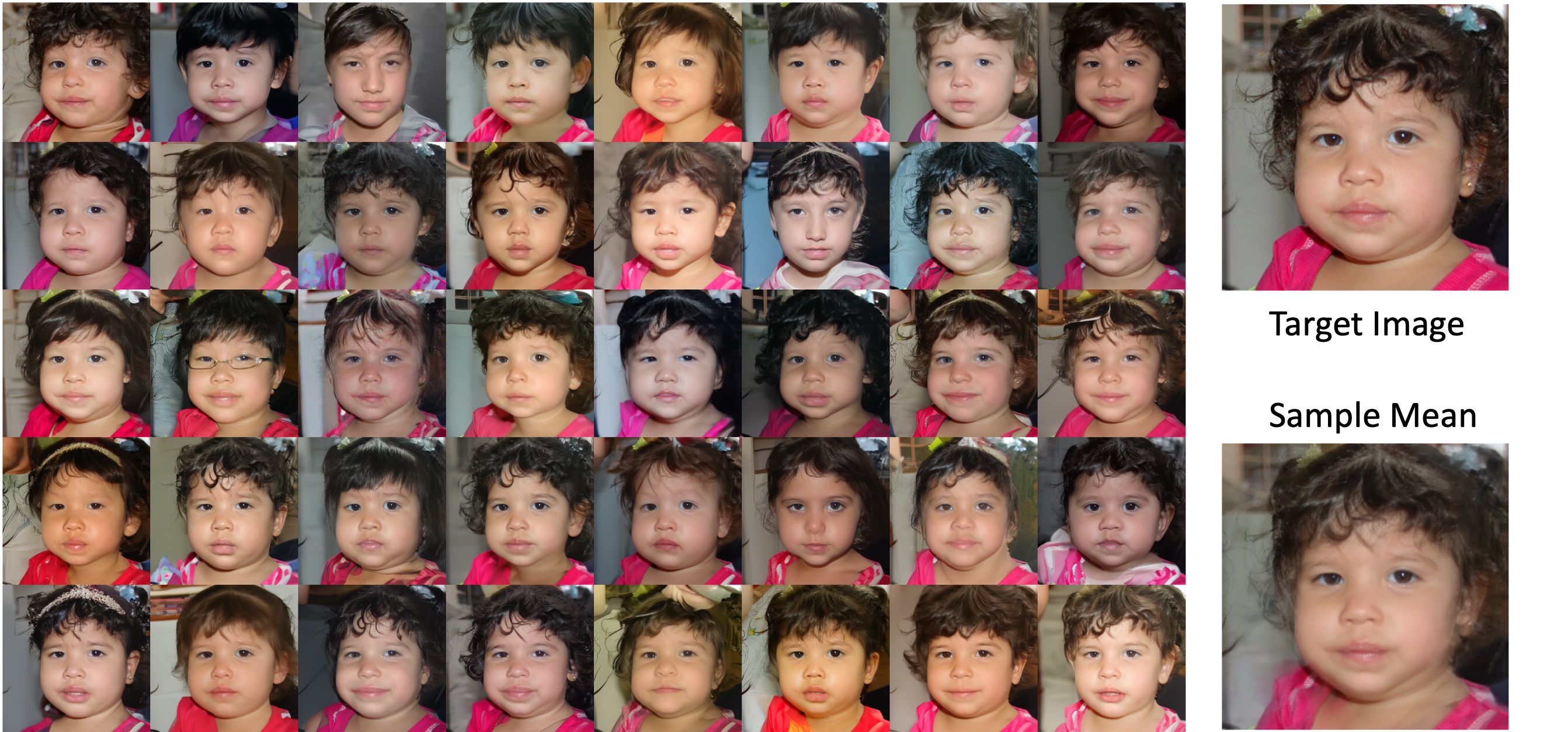
Figure 1: CCS Sampling with a target mean in the FFHQ validation dataset with $C_{0}=0.4$

Recently, diffusion models achieve remarkable success in generative tasks such as text-to-image generation, audio synthesis (Kong et al., ; Rombach et al., 2022), as well as conditional generation tasks including inverse problem solving, image or video restoration, image editing, and translation (Chen et al., 2024b; Liu et al., 2024; Zhang et al., 2023a; Chung et al., ; Song et al., ; Chung et al., 2023; Kwon & Ye, 2024; Song et al., 2023; He et al., ; Zhang et al., 2023b). Despite these success, real-world scientific and engineering problems pose more challenges on requesting reliable and controllable generation as well as data privacy.

To tackle this, one important question is: How to control the distribution of samples from a diffusion model to match a specific target? Previous works on controllable generation with diffusion models mostly focus on constraining the generation process sample-by-sample using either plug-and-play approaches (Narasimhan et al., 2024; Chung et al., 2023; Kwon & Ye, 2024; Song et al., 2023) or modifying the unconditional score (Rombach et al., 2022; Zhang et al., 2023b; Epstein et al., 2023; Chung et al., ), so that each sample can satisfy a measurement constraint. However, most prior works focus on per-sample control, with limited exploration of how to regulate the overall distribution of generated samples to meet specific statistical constraints, which is a crucial requirement in differential privacy (Dwork, 2006). This inspires the novel task for controllable and constrained sampling we are targeting in this paper. Considering the unique mechanism in diffusion sampling, we are motivated to exploit the initial noise control by studying this key question: How do the initial noise perturbations affect the generated samples in diffusion models? Previous works (Chen et al., ; Wang et al., 2024) suggest that the learned posterior mean predictor function is locally linear with perturbation among a certain range of timesteps for diffusion models. However, this linearity cannot be applied to every timestep nor to the samples of diffusion models. From a new perspective, this work sheds lights on the relationship between input noise perturbations and generation data in diffusion models, by proposing a training-free approach.

First of all, we observe an interesting phenomenon that when using denoising diffusion implicit models (DDIM) sampling, the initial noise has a highly linear effect on the generation data at small or moderate scales. Motivated by this observation, our study tries to justify this linearity property via initial noise perturbation theoretically and empirically.

Based on the spherical interpolation to perturb the initial noise vector, we propose a novel controllable and constrained sampling method (CCS) together with a new controller algorithm for diffusion models to sample with desired statistical properties while preserving high quality and adjustable diversity.

Furthermore, we conduct extensive experiments to validate the linearity phenomenon and then investigate the controllability performance of our proposed CCS method by generating images centered around a specified target mean image with a certain distance. Results demonstrate the superiority of our CCS method in both controllability and sampled image quality compared with baseline methods. Moreover, we show the potential of proposed CCS sampling for broader applications including image editing.

Our contributions can be summarized as below:

• To the best of our knowledge, we for the first time investigate a novel problem of controllable and constrained diffusion sampling, given constraints on certain statistical properties while preserving high sample quality.

• Motivated by our new finding on the highly linear relationship between the initial noise and generated samples, we propose an innovative noise perturbation method with a controller algorithm for constrained sampling around a target mean with a specified distance, supported by solid theoretical and empirical justifications.

• Extensive experiments on three datasets with both pixel and latent diffusion models, validate our findings and theoretical results about the linearity phenomenon and proposed algorithm. Results demonstrate the superior performance of our algorithm in achieving precise controllability within a constrained sampling framework.

2 Background

2.1 Diffusion Models

Diffusion models consists of a forward process that gradually adds noise to a clean image, and a reverse process that denoises the noisy images (Song et al., 2020; Song & Ermon, 2019). The forward model is given by $\mathbf{x}_{t}=\mathbf{x}_{t-1}-0.5\beta_{t}\Delta t\mathbf{x}_{t-1}+\sqrt{\beta_{t}}\Delta t\mathbf{\omega}$ where $\mathbf{\omega}\in\mathbb{N}(0,I)$ and $\beta(t)$ is the noise schedule of the process. The distribution of $\mathbf{x}_{0}$ is the clean data distribution, while the distribution of $\mathbf{x}_{T}$ is approximately a standard Gaussian distribution. When we set $\Delta t\rightarrow 0$, the forward model becomes $\mathrm{d}\mathbf{x}_{t}=-0.5\beta_{t}\mathbf{x}_{t}\mathrm{d}t+\sqrt{\beta_{t}}\mathrm{d}\omega_{t}$, which is a stochastic differential equation (SDE). The reverse of this SDE is given by:

$$\mathrm{d}x_{t}=\left(-\frac{\beta(t)}{2}-\beta(t)\nabla_{\mathbf{x}_{t}}\log p_{t}(\mathbf{x}_{t})\right)dt+\sqrt{\beta(t)}d\overline{\mathbf{\omega}}.$$

One can training a neural network to learn the score function $\nabla_{\mathbf{x}_{t}}\log p_{t}(\mathbf{x}_{t})$. However, this formulation involves running many timesteps with high randomness. We can also compute the equivalent Ordinary Differential Equation (ODE) form to the SDE, which has the same marginal distribution of $p(\mathbf{x}_{t})$. A sampling process, called denoising diffusion implicit models (DDIM), modifies the forward process to be non-markovian, so as to form a deterministic probability-flow ODE for the reverse process (Song et al., 2021). In this way, we are able to achieve significant speed-up sampling. More discussion on this can be found in Section 3.

2.2 Constrained Generation with Diffusion Models

Constrained generation requires to sample $\mathbf{x}_{0}$ subject to certain conditions or measurements $\mathbf{y}$. The conditional score at $T$ can be computed by the Bayes rule, such that

$$\nabla_{\mathbf{x}_{t}}\log p_{t}(\mathbf{x}_{t}|\mathbf{y})=\nabla_{\mathbf{x}_{t}}\log p_{t}(\mathbf{x}_{t})+\nabla_{\mathbf{x}_{t}}\log p_{t}(\mathbf{y}|\mathbf{x}_{t}).$$ (1)

The second term can be computed through classifier guidance (Dhariwal & Nichol, 2021a), where an external classifier is trained for $p_{0}(\mathbf{y}|\mathbf{x}_{0})$ or $p_{t}(\mathbf{y}|\mathbf{x}_{t})$, and then can be plug into the diffusion model through Eq. 1. Diffusion posterior sampling (Chung et al., ) further refines this formulation by proposing to perform posterior sampling with the approximation of $p(\mathbf{y}|\mathbf{x}_{t})\approx p(\mathbf{y}|\hat{\mathbf{x}}_{0})$, where $\hat{\mathbf{x}}_{0}$ is the Minimum Mean Square Error (MMSE) estimator of $\mathbf{x}_{0}$ based on $\mathbf{x}_{t}$.

Another line of works exploit hard consistency, which projects the intermediate noise to a measurement-consistent space during sampling via optimization and plug-and-play (Chung et al., 2022a, 2023; Narasimhan et al., 2024; Song et al., ). However, the projection term can damage the sample quality (Chung et al., ). However, these works all target on controlling each individual sample. To our best knowledge, few works explore how to control the distribution of generated samples to match certain statistical constraints, such as centered around a specified target mean with certain distance, which is the target for this work.

2.3 Noise Perturbation in Diffusion Models

Noise adjustment for diffusion models has been explored in image editing, video generation, and other applications (Liu et al., 2024; Zhang et al., 2023a; Chung et al., 2024; Guo et al., 2024; Wu & De la Torre, 2023; Zheng et al., 2024) for changing the style or other properties of the generated data. However, a principled study on how the noise adjustment affects the samples is limited in diffusion models. Recently, Chen et al. ; Wang et al. (2024) observe the local linearity and low-rankness of the posterior mean predictor $\mathbf{\hat{x}}_{0}$ based on $\mathbf{x}_{t}$ in large timesteps, but this study cannot extend to the analysis of generated samples. In this work, we investigate how initial noise perturbations affect the samples generated from the diffusion model in the ODE sampling setting.

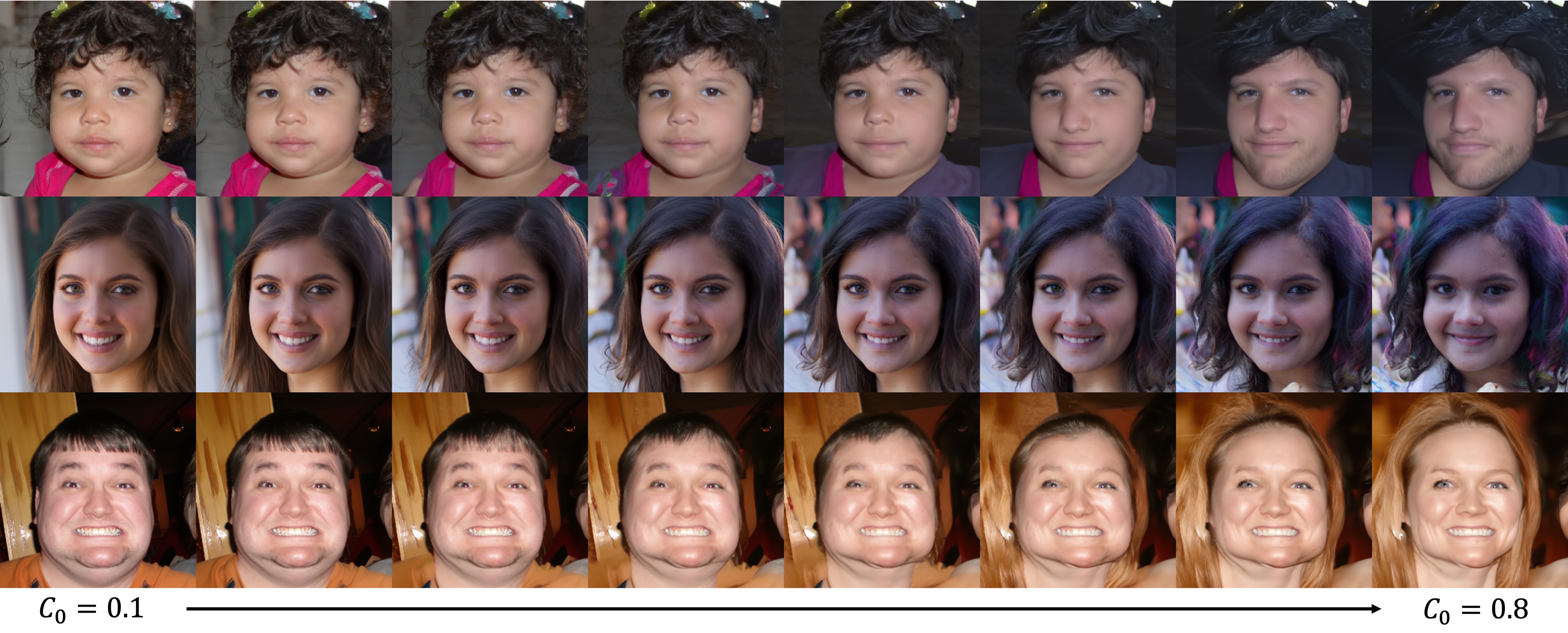
Figure 2: Qualitative demonstration of linearity when increasing scale of perturbation. For each target mean, we sample a perturbation noise and gradually increase $C_{0}$ (0.1 at a time) to increase the magnitude of the perturbation.

3 Influence from Initial Noise Perturbation

This section analyzes how small perturbations in the input noise affect the generation data under the DDIM sampling framework. We show that a slight change in the initial noise leads to an approximately linear variation in the sampled images. This result is quantified from two perspectives: the discretized DDIM sampling process (Song et al., 2021) and the associated continuous-time ODE. Our mathematical analysis relies on minimal assumptions, which also serves as the foundation for our proposed CCS algorithm in Section 4.

3.1 Preliminary: DDIM Sampling

Fix the total sampling timesteps $T$ and an initialization noise sample $\mathbf{x}_{T}$, Song et al. (2021) generates samples from the backward process $\mathbf{x}_{T}\rightarrow\mathbf{x}_{T-1}\rightarrow\ldots\rightarrow\mathbf{x}_{0}$ using the following recursive formula:

$$\mathbf{x}_{t-1}=\sqrt{\alpha_{t-1}}\left(\frac{\mathbf{x}_{t}-\sqrt{1-\alpha_{t}}\,\epsilon_{\theta}^{(t)}(\mathbf{x}_{t})}{\sqrt{\alpha_{t}}}\right)$$ (2)

$$+\sqrt{1-\alpha_{t-1}-\sigma_{t}^{2}}\,\epsilon_{\theta}^{(t)}(\mathbf{x}_{t})+\sigma_{t}\epsilon_{t},$$

where $\alpha_{t}$ corresponds to the noise schedule in DDPM, $\epsilon_{\theta}^{(t)}(\mathbf{x}_{t})$ is the predicted noise given by the pre-trained neural network with parameter $\theta$, $\epsilon_{t}$ is the standard Gaussian noise, and $\sigma_{t}$ is a hyperparameter. The DDIM sampler (Song et al., 2021) sets $\sigma_{t}=0$ to make the backward process deterministic once $\mathbf{x}_{T}$ is fixed. It is known (e.g., eq (11) of Dhariwal & Nichol (2021b)) that predicting the noise is equivalent to predicting the score function up to a normalizing factor, i.e., $\epsilon_{\theta}^{(t)}\left(\mathbf{x}_{t}\right)\approx-\sqrt{1-\alpha_{t}}\nabla_{\mathbf{x}_{t}}\log p_{t}(\mathbf{x}_{t})$. By setting $\sigma_{t}=0$ and substituting $\epsilon_{\theta}^{(t)}$ with its corresponding estimand, we obtain the idealized DDIM process:

$$\mathbf{x}_{t-1} =\sqrt{\alpha_{t-1}}\left(\frac{\mathbf{x}_{t}+(1-\alpha_{t}\,)\nabla_{\mathbf{x}_{t}}\log p_{t}(\mathbf{x}_{t})}{\sqrt{\alpha_{t}}}\right)$$ (3)

$$~~~~-\sqrt{(1-\alpha_{t-1})(1-\alpha_{t})}\,\nabla_{\mathbf{x}_{t}}\log p_{t}(\mathbf{x}_{t}).$$

If we treat the index $t$ as a continuous variable (and rewrite $\alpha_{t}$ as $\alpha(t)$ to avoid confusion), it is known in eq (14) of (Song et al., 2020) that DDIM is the Euler-discretization of the following (backward) ODE:

$$\mathrm{d}\bar{\mathbf{x}}_{t}=\epsilon_{\theta}^{(t)}\left(\frac{\bar{\mathbf{x}}_{t}}{\sqrt{\sigma^{2}(t)+1}}\right)\mathrm{d}\sigma(t),$$

where $\bar{\mathbf{x}}_{t}=\mathbf{x}_{t}/\sqrt{\alpha(t)},\sigma(t):=\sqrt{(1-\alpha(t))/\alpha(t)}.$ Thus, we can similarly write the idealized ODE as:

$$\mathrm{d}\bar{\mathbf{x}}_{t}=-\sqrt{1-\alpha(t)}\nabla\log p_{t}\left(\frac{\bar{\mathbf{x}}_{t}}{\sqrt{\sigma^{2}(t)+1}}\right)\mathrm{d}\sigma(t).$$ (4)

We now examine how a small perturbation $\mathbf{x}_{T}\rightarrow\mathbf{x}_{T}+\lambda\Delta\mathbf{x}$ would affect the output sample at time $t=0$ through both the discrete (3) and continuous time (4) perspectives.

Related work: Theorem 1 in Chen et al. (2024b) presents a related result on the impact of initial noise perturbation. Our study differs from theirs in a variety of aspects. Firstly, they study $\mathbb{E}[\mathbf{x}_{0}\mid\mathbf{x}_{t}+\lambda\Delta\mathbf{x}]-\mathbb{E}[\mathbf{x}_{0}\mid\mathbf{x}_{t}]$ under the (stochastic) diffusion process. In contrast, we directly examine the output $\mathbf{x}_{0}$ given the initializations $\mathbf{x}_{t}$ and $\mathbf{x}_{t}+\lambda\Delta\mathbf{x}$ under the deterministic DDIM (3) or the ODE process (4). Secondly, (Chen et al., 2024b) assumes that $p_{0}$ is a low-rank mixture of Gaussian distributions, which allows for an analytical solution for $p_{t}$. In contrast, our weaker assumptions render $p_{t}$ analytically intractable. Consequently, we use very different techniques, such as ODE stability theory and Grönwall’s inequality, to study the system’s behavior.

3.2 DDIM Discretization

We simplify notations and write the idealized DDIM (3) as

$$\mathbf{x}_{t-1}:=\eta_{t}\mathbf{x}_{t}+\lambda_{t}\nabla_{\mathbf{x}_{t}}\log p_{t}(\mathbf{x}_{t}),$$

where $\eta_{t}=\sqrt{\alpha_{t-1}^{-1}\alpha_{t}}$ and $\lambda_{t}=\sqrt{\alpha_{t-1}^{-1}\alpha_{t}}(1-\alpha_{t})-\sqrt{(1-\alpha_{t-1})(1-\alpha_{t})}$.

Fix $T$, we are interested in studying $\mathbf{x}_{0}(\mathbf{x}_{T},T)$ and $\mathbf{x}_{0}(\mathbf{x}_{T}+\lambda\Delta\mathbf{x},T)$, where $\Delta\mathbf{x}$ is a unit direction and $\lambda$ is a (small) real number. The notation $\mathbf{x}_{0}(a,t)$ stands for the endpoint $\mathbf{x}_{0}$ by applying the idealized DDIM procedure with $\mathbf{x}_{t}=a$ at timestep $t$. We have:

Proposition 1.

With all the notations defined as above, assuming $\log p_{t}$ is second-order differentiable for every $t\geq 1$, there exists a matrix-valued function $\gamma_{0}$ such that

$$\mathbf{x}_{0}(\mathbf{x}_{T}+\lambda\Delta\mathbf{x},T)=\mathbf{x}_{0}(\mathbf{x}_{T})+\lambda\gamma_{0}(\mathbf{x}_{T})\Delta\mathbf{x}+o(\lambda).$$

In turn,

$$\lVert\mathbf{x}_{0}(\mathbf{x}_{T}+\lambda\Delta\mathbf{x},T)-\mathbf{x}_{0}(\mathbf{x}_{T},T)\rVert_{2}$$

$$=\lVert\lambda\gamma_{0}(\mathbf{x}_{T})\Delta\mathbf{x}\rVert_{2}+o(\lambda).$$

Proposition 1 shows that a linear perturbation of the input with magnitude $\lambda$ and direction $\Delta\mathbf{x}$ results in an approximately linear change in the output, with magnitude $\lvert\lambda\rvert\lVert\gamma_{0}(\mathbf{x}_{T})\Delta\mathbf{x}\rVert_{2}$ and direction $\gamma_{0}(\mathbf{x}_{T})\Delta\mathbf{x}$. Our assumption is based solely on the second-order smoothness of the score, which is weaker than most existing assumptions depending on the data distribution $p_{0}$. For example, our assumptions hold under common conditions in the literature, such as the manifold hypothesis (De Bortoli, 2022; Song & Ermon, 2019) or the mixture of (low-rank) Gaussian assumption (Gatmiry et al., 2024; Chen et al., 2024b, a).
Furthermore, when at large $t$, $p_{t}$ is approximately Gaussian and $\nabla_{\mathbf{x}_{t}}\text{log}p_{t}(\mathbf{x}_{t})$ is smooth, which leads to low linear approximation error. However, one might be concerned that the linear approximation error could grow significantly when $t$ decreases and $p_{0}$ contains multiple clusters with low-density regions in between. Nevertheless, we now explain why this concern does not arise in practice. The coefficient $f(t):=-\sqrt{\alpha_{t}}^{-1}\sqrt{\alpha_{t-1}(1-\alpha_{t})}+\sqrt{1-\alpha_{t-1}}$ of $\epsilon_{\theta}^{(t)}(\mathbf{x}_{t})$ in (2) is close to $0$ for small $t$, as $\alpha_{t}\approx 1$. Moreover, the structure of the neural network $\epsilon_{\theta}$ ensures that the output is normalized and bounded in norm, so the change in output is also bounded. Consequently, for a small perturbation in $\mathbf{x}_{t}$, we have $\lVert f(t)(\epsilon_{\theta}^{(t)}(\mathbf{x}_{t}+\Delta x)-\epsilon_{\theta}^{(t)}(\mathbf{x}_{t}))\rVert_{2}\approx 0$ when $t$ is small.

3.3 ODE Stability

Let $\bar{\mathbf{x}}_{0}(\mathbf{x},T)$ be the solution of (4) with initialization $\mathbf{x}_{T}=\mathbf{x}$ (i.e., $\bar{\mathbf{x}}_{T}=\mathbf{x}/\sqrt{\alpha(T)}$) at timestep $T$, and $x_{0}(\mathbf{x},T)=\alpha(0)\bar{\mathbf{x}}_{0}(\mathbf{x},T)$. With some technical assumptions that is detailed in Appendix A.2, we have the following:

Proposition 2.

There exists a matrix-valued function $\psi_{0}$ such that:

$$\bar{\mathbf{x}}_{0}(\mathbf{x}_{T}+\lambda\Delta\mathbf{x},T)=\bar{\mathbf{x}}_{0}(\mathbf{x}_{T})+\lambda\psi_{0}(\mathbf{x}_{T})\Delta\mathbf{x}+o(\lambda).$$

In turn,

$$\mathbf{x}_{0}(\mathbf{x}_{T}+\lambda\Delta\mathbf{x},T)=\mathbf{x}_{0}(\mathbf{x}_{T})+\lambda\sqrt{\alpha(0)}\psi_{0}(\mathbf{x}_{T})\Delta\mathbf{x}+o(\lambda).$$

Proposition 2 mirrors Proposition 1 but is formulated in the continuous-time ODE setting. Its proof relies on ODE stability theory, showing that the output change is “approximately linear” for sufficiently small $\lambda$. Furthermore, under the same assumption, we establish that the change remains “at most linear” for all $\lambda$. The proof, which applies Grönwall’s inequality, is provided in Appendix A.2.

Proposition 3.

With the same assumptions as above, there exists a constant $C(T)$ depending on $T$ such that for any $\lambda$:

$$\lVert\bar{\mathbf{x}}_{0}(\mathbf{x}_{T}+\lambda\Delta\mathbf{x},T)-\bar{\mathbf{x}}_{0}(\mathbf{x}_{T})\rVert_{2}\leq C(T)\lvert\lambda\rvert\lVert\Delta\mathbf{x}\rVert_{2}.$$

4 Sampling with Control

Now we discuss our controllable sampling algorithm. We preserve the notation $\mathbf{x}_{0}$ to denote a “target image” or “target mean” (e.g., the top right corner in Figure 1). We also preserve the notation $\mathbf{x}_{T}:=\text{DDIM}^{-1}(\mathbf{x}_{0};0,T)$, the “noise” by running DDIM (2) reversely from time $0$ to $T$. Our objective is to perturb $\mathbf{x}_{T}$ into a random $\mathbf{x}_{T}^{\prime}$ such that the generated image $\mathbf{x}_{0}^{\prime}$ such that it has 1. a sample mean close to $\mathbf{x}_{0}$ while maintaining 2. sufficient diversity and difference from the original image and 3. high image quality. The closeness is quantified by $L$-2 norm distance $\rVert\mathbb{E}[\mathbf{x}_{0}^{\prime}]-\mathbf{x}_{0}\rVert_{2}$, and the diversity is measured by $\mathbb{E}[||\mathbf{x}_{0}^{\prime}-\mathbf{x}_{0}||_{2}^{2}]$. A notable feature of our algorithm is that users can specify a desired level of diversity ($C_{0}$ in Fig. 1, 2), and the generated images will match this level while ensuring $\mathbb{E}[\mathbf{x}_{0}^{\prime}]\approx\mathbf{x}_{0}$. Our mechanism is defined as $\mathbf{x}_{T}^{\prime}=a\mathbf{x}_{T}+b\Delta$, where $\Delta$ is a random perturbation, and $a$ and $b$ are parameters to be specified shortly.

4.1 Sampling around a Center

For an input of the form $\mathbf{x}^{\prime}_{T}=a\mathbf{x}_{T}+b\Delta$ with random $\Delta$, when $b$ is small and $a$ is close to 1, it can be regarded as a slight perturbation of $\mathbf{x}_{T}$. Based on Section 3, the output will remain close to $\mathbf{x}_{0}$ with an additional linear adjustment applied to $b\mathbf{n}$. Thus, we define $\hat{\mathbf{x}}_{0}^{\prime}:=\mathbf{x}_{0}+bA\Delta$ as an approximation for $\mathbf{x}_{0}^{\prime}$, where $A=\gamma_{0}(a\mathbf{x}_{T}+b\Delta)$ specified in Proposition 1. Since $\Delta$ is the only source of randomness in $\hat{\mathbf{x}}_{0}^{\prime}$, we can easily calculate $\mathbb{E}[\hat{\mathbf{x}}_{0}^{\prime}]=\mathbf{x}_{0}+bAE[\Delta]$ and $\operatorname{Var}[\hat{\mathbf{x}}_{0}^{\prime}]=b^{2}A\operatorname{Cov}(\Delta)A^{\top}$. We will now discuss the principles for our sampling design.

High-quality image generation: we first note that the input to both DDPM and DDIM samplers is standard Gaussian noise. The following feature is known as the “concentration phenomenon” of a high-dimensional Gaussian:

Proposition 4.

Let $X\sim\mathbb{N}(0,I_{d})$, then for any $\delta\in(0,1)$

$$\mathbb{P}\left[\lVert X\rVert_{2}^{2}\in(1\pm\delta)d\right\rvert]\geq 1-2\exp\left(-\frac{1}{2}d\left(\frac{1}{2}\delta^{2}-\frac{1}{3}\delta^{3}\right)\right).$$

This result suggests that a standard Gaussian noise vector remains close to a hypersphere of radius $\sqrt{d}$. For example, when $d=50{,}000$ (a common dimension in imaging) and $\delta=0.025$, Proposition 4 guarantees with over 99.9% probability that the squared norm is in the interval $\bigl{(}0.975\,d,\;1.025\,d\bigr{)}$. Empirical results (Song et al., 2020) further confirm that starting with a noise vector on this hypersphere is important for generating high-quality images.

Hence, we can expect $\lVert\mathbf{x}_{T}\rVert_{2}\approx\sqrt{d}$. Furthermore, we will design our mechanism to ensure $\mathbf{x}^{\prime}_{T}$ also has a norm $\approx\sqrt{d}$.

Close to target mean: Our approximation $\hat{\mathbf{x}}_{0}^{\prime}$ has expectation $\mathbb{E}[\hat{\mathbf{x}}_{0}^{\prime}]=\mathbf{x}_{0}+bAE[\Delta]$. Thus, it is sufficient to select $\Delta$ such that $\mathbb{E}[\Delta]=0$ in order to achieve: $\mathbb{E}[\hat{\mathbf{x}}_{0}]\approx\mathbb{E}[\hat{\mathbf{x}}_{0}^{\prime}]=\mathbf{x}_{0},$ where the first approximation is justified by Proposition 1 and 2, and is empirically validated in Figure 9.

4.2 Centering Feasibility

The simplest strategy is to add a random noise vector $\Delta\mathbf{x}$ directly to $\mathbf{x}_{T}$, expressed as $\mathbf{x}_{T}^{\prime}=\mathbf{x}_{T}+\Delta\mathbf{x}$ (with $a=1,b\Delta=\Delta\mathbf{x}$). However, the following proposition demonstrates that this approach cannot produce high-quality images.

Proposition 5.

For any fixed vector $\mathbf{x}$, and any random vector $\Delta\mathbf{x}$ such that $\mathbb{E}[\Delta\mathbf{x}]=0$, the following holds:

$$\mathbb{E}[\lVert\mathbf{x}+\Delta\mathbf{x}\rVert_{2}^{2}]=\lVert\mathbf{x}\rVert^{2}_{2}+\operatorname{tr}(\operatorname{Cov}[\Delta\mathbf{x}])\geq\lVert\mathbf{x}\rVert_{2}^{2},$$

with equality if and only if $\Delta\mathbf{x}=0$ almost surely.

Proposition 5 indicates that directly adding noise, $\mathbf{x}_{T}\rightarrow\mathbf{x}_{T}^{\prime}:=\mathbf{x}_{T}+\Delta\mathbf{x}$, pushes $\mathbf{x}_{T}^{\prime}$ farther from the spherical surface. This partly explains why the average image becomes blurrier or noisier as the scale of $\Delta\mathbf{x}$ increases, since the drift term $\operatorname{tr}(\operatorname{Cov}[\Delta\mathbf{x}])$ grows larger, causing $\mathbf{x}_{T}^{\prime}$ to deviate further from the sphere with radius $\lVert\mathbf{x}_{T}\rVert_{2}$.

This inspires us to consider the spherical linear interpolation method (Shoemake, 1985) for sampling, as described below. Similar approaches have been proposed by  (Zheng et al., 2024; Song et al., 2020), but only for interpolating between two images.

4.3 Spherical Interpolation

Let vectors $\mathbf{a}$ and $\mathbf{b}$ satisfy $\lVert\mathbf{a}\rVert_{2}=\lVert\mathbf{b}\rVert_{2}$ and form an angle $\theta$. Then for any $\alpha\in(0,1)$, the vector obtained through spherical interpolation $\mathbf{c}:=\frac{\sin(\alpha\theta)}{\sin\theta}\mathbf{a}+\frac{\sin((1-\alpha)\theta)}{\sin(\theta)}\mathbf{b}$ satisfies $\lVert\mathbf{c}\rVert_{2}=\lVert\mathbf{a}\rVert_{2}=\lVert\mathbf{b}\rVert_{2}$.

In our case, for a standard $d$-dimensional normal noise vector $\mathbf{\epsilon}$, it is known $\lVert\mathbf{\epsilon}\rVert_{2}\approx\sqrt{d}\approx\lVert\mathbf{x}_{T}\rVert_{2}$. Therefore, we can do spherical interpolation between $\mathbf{x}_{T}$ and $\mathbf{\epsilon}$ to obtain $\mathbf{x}_{T}^{\prime}$. Our CCS algorithm is described in Algorithm 1.

The perturbation mechanism corresponds to $\mathbf{x}_{T}^{\prime}=a\mathbf{x}_{T}+b\Delta$ with $a=\sin(\theta-C_{0})/\sin(\theta),b=\sin(C_{0})/\sin(\theta),\Delta=\epsilon\sim\mathbb{N}(0,I)$. $C_{0}:=\alpha\theta$ is defined as the parameter of perturbation scale. This mechanism satisfies the design principles described in Section 4.1: $\mathbb{E}[\mathbf{\epsilon}]=0$ ensures that the new sample remains close to the target mean, while the Gaussian concentration and spherical interpolation ensure that $\lVert\mathbf{x}_{T}^{\prime}\rVert_{2}\approx\lVert\mathbf{x}_{T}\rVert_{2}$, resulting in high-quality generated images.

Algorithm 1 (Full Inversion) CCS Sampling

Requires: target mean $\mathbf{x}_{0}$, perturbation scale $C_{0}$, number of diffusion model timesteps $T$

Step 0: Compute the DDIM inversion of $\mathbf{x}_{0}$, i.e. $\mathbf{x}_{T}=\text{DDIM}^{-1}(\mathbf{x}_{0},0,T)$

Step 1: Sample noise $\epsilon\sim\mathbb{N}(0,I)$. Then compute

$$\theta=\cos^{-1}\left(\frac{\epsilon\cdot\mathbf{x}_{T}}{||\epsilon||_{2}||\mathbf{x}_{T}||_{2}}\right)$$

Step 2: Compute $\mathbf{x}_{T}$ using spherical interpolation formula:

$$\mathbf{x}_{T}^{\prime}=\frac{\sin(C_{0})}{\sin(\theta)}\cdot\epsilon+\frac{\sin(\theta-C_{0})}{\sin(\theta)}\cdot\mathbf{x}_{T}$$

Step 3: Output sample $\mathbf{x}_{0}^{\prime}=\text{DDIM}(\mathbf{x}_{T}^{\prime},T,0)$

Parameter $C_{0}$ controls sampling diversity. In the extreme case $C_{0}=0$, we have $\mathbf{x}_{T}^{\prime}=\mathbf{x}_{T}$, so $\mathbf{x}_{0}^{\prime}$ matches $\mathbf{x}_{0}$ exactly but has no diversity. A larger $C_{0}$ makes the perturbed input deviate more from the original image and gets closer to noise. This leads to greater diversity in the generated image.

Algorithm 2 allows users to control the desired level of diversity. It works by calling Algorithm 1 for different values of $C_{0}$, which are determined through binary search. Let The process is repeated until the desired diversity level (up to a small tolerance threshold) is reached: if the MSE of generated images to target mean is below target threshold, $C_{0}$ is increased; otherwise, it is decreased.

Algorithm 2 Controller Tuning (CT)

1: Input: target mean $\mathbf{x}_{0}$, target diversity level ${\text{MSE}}_{\text{target}}$, tolerance: tol

2: Initialize: $C_{\text{low}}\leftarrow 0$, $C_{\text{high}}\leftarrow\pi/2$, $C_{0}\leftarrow\frac{C_{\text{low}}+C_{\text{high}}}{2}$

3: while not converged do

4:  Sample a batch of $\mathbf{x}_{0}^{\prime}$ by Alg. 1 with $C_{0}$ and $\mathbf{x}_{0}$

5:  if $|\mathbb{E}[||\mathbf{x}_{0}^{\prime}-\mathbf{x}_{0}||_{2}]-{\text{MSE}}_{\text{target}}|<{\text{tol}}$ then

6:   Break

7:  else if $\mathbb{E}[||\mathbf{x}_{0}^{\prime}-\mathbf{x}_{0}||_{2}]>{\text{MSE}}_{\text{target}}$ then

8:   $(C_{\text{high}},C_{0})\leftarrow(C_{0},\frac{C_{0}+C_{\text{low}}}{2})$

9:  else

10:   $(C_{\text{low}},C_{0})\leftarrow(C_{0},\frac{C_{0}+C_{\text{high}}}{2})$

11:  end if

12: end while

The following theorem demonstrates that the CCS algorithm is able to precisely control the input distance.

Proposition 6.

Denote the dimensionality of $\mathbf{x}_{T}$ by $d$. Given an initial noise $\mathbf{x}_{T}$ with $\lVert\mathbf{x}_{T}\rVert_{2}=(1+o(1))\sqrt{d}$, and fix a small $\delta>0$. For any $M\leq(2-\delta)\sqrt{d}$, then we can find $C_{0}$ in Algorithm 1 such that with probability $p_{d}\rightarrow 1$ as $d\rightarrow\infty$, we have $\lVert\mathbf{x}_{T}^{\prime}-\mathbf{x}_{T}\rVert_{2}=M$.

Since the dimensionality of our problem is sufficiently large, Proposition 6 allows users to control $M$ as the input distance. Consequently, Algorithm 1 can generate a random interpolants with an exact distance of $M$ from the input. Furthermore, since the direction is uniformly distributed, and when $C_{0}$ is small, $\mathbb{E}[\mathbf{x}_{T}^{\prime}]\approx\mathbb{E}[\mathbf{x}_{T}]$, and $\mathbb{E}[\mathbf{x}_{0}^{\prime}]\approx\mathbb{E}[\mathbf{x}_{0}]$, which satisfies our design goal.

4.4 Extension to Conditional Latent Diffusion Models

Conditional diffusion models usually compute the conditional score with classifier-free guidance (CFG). Let $s_{\theta}(\mathbf{x}_{t},t)$ be the predicted noise, it can be written in $s_{\theta}(\mathbf{x}_{t},t)=s_{\theta}(\mathbf{x}_{t},t,c_{null})+\gamma(s_{\theta}(\mathbf{x}_{t},t,c)-s_{\theta}(\mathbf{x}_{t},t,c_{null}))$ where $\gamma$ is the CFG term, $c$ is the condition and $c_{null}$ is the null condition. Exact inversion is very challenging in a high CFG setting (Hong et al., 2024), and reconstruction error in the autoencoder of latent diffusion models makes it even harder. Motivated by this, we propose a Partial-Inversion CCS Sampling algorithm (P-CCS). Instead of starting from the $T$, we pick an intermediate timestep $t_{0}$. Then, we compute the noise term from DDIM inversion by subtracting the clean component, sample a new noise from $\mathbb{N}(0,(1-\alpha_{t_{0}})I)$, and then perform spherical interpolation. Details of this Alg. 3 can be found in the Appendix. Furthermore, we can sample around a edited target mean by first performing DDIM inversion with source prompt, then apply P-CCS sampling, and finally run DDIM with target prompt. More details can be found in the experiments and the Appendix.

5 Experiments

In the experiments, we aim to answer three questions: 1. Can we sample images that have a sample mean close to the target mean with a target MSE by our designed algorithms while maintaining good image quality? 2. Does the linearity phenomenon between the norm of residual images and the perturbation scale widely exist? 3. Can our proposed algorithm work in more challenging settings such as in conditional generation with CFG or image editing tasks?

5.1 Validation of Linearity Phenomenon

Experimental setting. We perform extensive experiments on both pixel diffusion models on the FFHQ and CIFAR-10 dataset and latent diffusion models on the Celeba-HQ and fMoW dataset. For each experiment, we first sample 50 images as target images from each validation dataset from FFHQ (Karras, 2019), CIFAR-10(Krizhevsky et al., 2009), and Celeba-HQ (Xia et al., 2021). We also pick one images each class from the validation set of the fMoW dataset (Christie et al., 2018) for further verification. Then for the FFHQ and CIFAR-10 selected data, we use pixel diffusion models as backbone; for Celeba-HQ and fMoW we use stable diffusion 1.5 as the backbone. The prompt for Celeba-HQ is given by ”A high quality photo of a face” and the prompt for fMoW is given by ”satellite images”. Then, we use each image as a target mean and perform CCS sampling as in Alg.1.

For each target image, we sample eight $C_{0}$ from a uniform [0, 0.9] distribution. For each $C_{0}$, we sample 24 images. Then we compute the average $L^{2}$ distance between the sampled images and the target mean for each scale.

Evaluations. To quantitatively evaluate the linearity phenomenon, we compute the R-square between the input perturbation scales and the normalized average residual norms (scale between 0-1) for 4 datasets with both pixel diffusion models and latent diffusion models. Note that since different target means can lead to different slopes by different Hessian matrices, we normalize the residual norms. Specifically, we compute empirical slope $a$ and bias $b$ between $x=\sin(C_{0})$ and $y=\mathbb{E}[\lVert\mathbf{x}_{0}^{\prime}-\mathbf{x}_{0}\rVert_{2}]$ each target mean, and then normalize the average $L^{2}$ distance to be: $y^{\prime}=\frac{y-b}{a}$.

Results. We observe a very strong linearity in the above experiments. Especially for pixel diffusion models, the R-square exceeds 0.98 for both datasets, which indicates almost a perfect linear relationship. For latent diffusion models, the linearity is slightly weaker, but still above 0.94 in R-square for both datasets. This is expected since Stable Diffusion use a nonlinear autoencoder and trained on a different dataset. We also present more quantitative results in Fig. 3 and qualitative results in Fig. 2. Surprisingly, we also observe a very linear semantic change in additional to pixel-value change.

Pixel Diffusion Models		Latent Diffusion Models
FFHQ	CIFAR-10	CelebA-HQ	fMoW
0.995	0.988	0.959	0.947

Table 1: R-square between scales of input perturbation and normalized residual norms

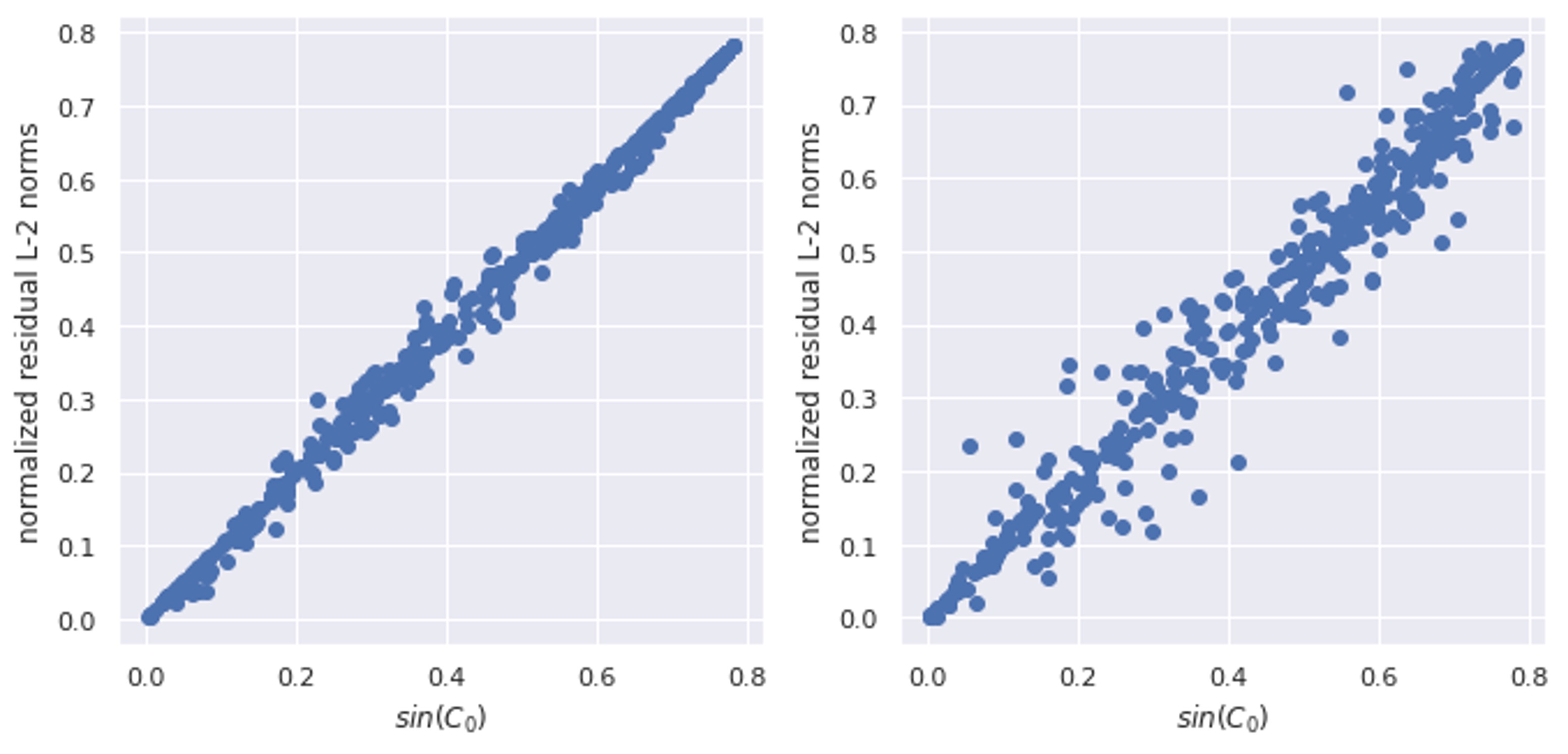
Figure 3: Quantitative demonstration of linearity when increasing scale of perturbation. With increased $\sin(C_{0})$, the magnitude of perturbation increases, and the average $L^{2}$ distance between samples and the target image increases linearly. Left is the linearity on FFHQ dataset using pixel diffusion; Right is the linearity on Celeba-HQ dataset using Stable Diffusion 1.5.

5.2 Controllable Sampling

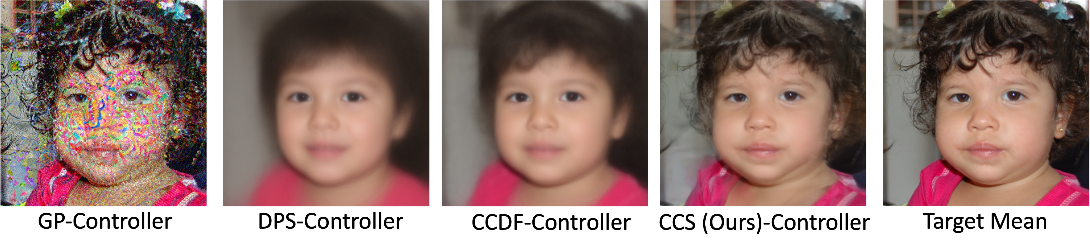
Figure 4: We sample 120 images with a fixed target mean using different methods and analyze their sample mean (average pixel intensity). Our observations show that the sample mean of our method closely matches that of the original image.

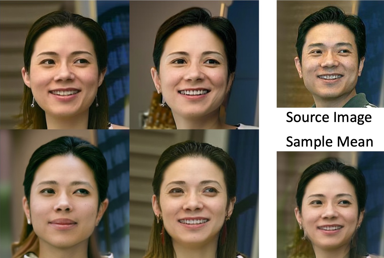
Figure 5: Example Samples of P-CCS around an Edited Mean.

Experimental setting. For pixel diffusion models, we use the first 50 images from the validation data from the FFHQ-256 (Chung et al., ) dataset. Then we set each image as the target mean and then sample 120 images (6000 images in total) with each target mean with a target rMSE (square root of average L-2 norm of the residuals between the sample and target mean) of 0.12. Then we test on the CIFAR-10 dataset. We randomly sample 20 images serving as target means, and then sample 120 images for each target mean with a target rMSE level of 0.11.

For Stable Diffusion, we use the SD1.5 checkpoint (Rombach et al., 2022). We study a more challenging scenario (degraded low-resolution input images with conditional text-guided latent diffusion model). We sample 50 images from the validation set from Celeba-HQ dataset with resolution $256\times 256$, and then use bicubic upsampling to upscale it to $512\times 512$. Note that SD1.5 is not trained on the Celeba-HQ dataset so this demonstrates the generalization capability of algorithms. We use the same prompt and CFG level in the linearity control experiments.

Implementation details. We follow Alg. 1 in implementing our methods for pixel diffusion models, and Alg. 3 for latent diffusion models. We take the pretrained models for FFHQ and CIFAR-10 from the improved/guided diffusion repos (Nichol & Dhariwal, 2021; Dhariwal & Nichol, 2021a) for the pixel diffusion experiments, and the Stable Diffusion 1.5 (Rombach et al., 2022) for latent diffusion experiments. For LDMs, we set $t_{0}=45$, where $T=50$ due to DDIM inversion performing worse with classifier-free guidance than unconditional models. We set the rMSE target to be 0.12, 0.11 for FFHQ and CIFAR-10 respectively, and 0.07 for Stable Diffusion experiments to test diverse control targets. The tolerance is set to be 0.01 in all cases. More details in the Appendix.

Baselines. Since we target task is quite novel task without existing method may serve as exact baseline to compare with, we have to adapt some previous methods with our proposed controller algorithm as an add-on to this new setting.

• Gaussian Perturbation with Controller (GP-C): We add a Gaussian perturbation to the initial noisy image $x_{t0}$, where the perturbation scale is determined by our controller. This method resembles works that perform local editing (Chen et al., ).

• (Latent) Diffusion Posterior Sampling (Chung et al., ; Song et al., ) with controller (DPS-C): We perform posterior sampling with $x_{0}$ as the measurement. The scale of the gradient term in (L)DPS can control the randomness, so we design a controller based on this. Details in the Appendix.

• ILVR with controller (ILVR-C): the ILVR algorithm (Choi et al., 2021) is for sampling high quality images based on a reference image. The larger the downsampling parameter gives a better diversity, we dynamically adjust that parameter as by our controller algorithm. Since it is designed only for DDPM, we do not experiment it with LDMs. Details in the Appendix.

• Come-closer-diffuse-faster with controller (CCDF-C): CCDF use DDPM forward to find a starting noise at $t_{0}$, and then perform reverse sampling based on that noise (Chung et al., 2022b). We adjust $t_{0}$ based on our controller algorithm.

Evaluation metrics. We first compute pixel-wise metrics to validate our hypothesis that sample mean is close to the target mean.

• PSNR (Peak Signal-to-Noise Ratio): quantifies the pixel-wise difference between the target mean and the sample mean.

• SD: the average of standard deviations of pixel intensities for each sampled image, which is used to measure the diversity of images.

Then we compute perceptual and reference-free metrics to measure the sample quality:

• MUSIQ (Ke et al., 2021): measures the perceptual image quality, which focuses on low-level perceptual quality and is sensitive to blurs/noise/other distortions

• CLIP-IQA (Wang et al., 2023): measures the semantic image quality, which is more higher-level than MUSIQ

• Inception Score (IS) (Salimans et al., 2016): is used in the CIFAR-10 dataset to further measure image quality and diversity. Since CIFAR-10 has a low resolution and images are blurry, we report IS score instead of MUSIQ and CLIP-IQA for CIFAR-10.

Results. Quantitative results are demonstrated in Table. 2, 3, 4. We observe that our CCS sampling method significantly outperforms all other methods in centering at a target mean when fixing the MSE level, while surprisingly maintaining superior image perceptual quality and diversity. Posterior sampling methods suffer from image quality degradation and diversity decreases. Qualitatively, we observe that the sample means of other methods look blurry or noisy, as demonstrated in Fig. 4. Note that although GP satisfies $\mathbb{E}[\Delta x]=0$, it pushes $\mathbf{x}_{T}^{\prime}$ further from the spherical surface, where the diffusion model is not trained on. Empirically we observe very noisy samples and sample mean.

Methods	PSNR$\uparrow$	SD$\uparrow$	CLIP-IQA$\uparrow$	MUSIQ$\uparrow$
GP-C	18.88	0.028	0.701	45.88
ILVR-C	20.04	0.070	0.746	62.45
DPS-C	21.02	0.069	0.738	64.60
CCDF-C	23.52	0.088	0.746	66.15
CCS (Ours)-C	25.13	0.104	0.750	66.79

Table 2: Results of Pixel Diffusion models on the FFHQ Dataset with rMSE target 0.12.

Methods	PSNR$\uparrow$	SD$\uparrow$	IS$\uparrow$
GP-C	24.66	0.100	7.56
DPS-C	23.13	0.054	7.86
CCDF-C	24.63	0.099	7.91
CCS (Ours)-C	26.05	0.107	8.09

Table 3: Results of Pixel Diffusion models on the CIFAR-10 Dataset with rMSE target 0.11.

Methods	PSNR$\uparrow$	SD$\uparrow$	CLIP-IQA$\uparrow$	MUSIQ$\uparrow$
GP-C	23.02	0.045	0.721	48.91
LDPS-C	24.56	0.034	0.721	29.07
CCDF-C	27.66	0.051	0.735	49.29
CCS (Ours)-C	30.29	0.053	0.732	49.66

Table 4: Results of the Stable Diffusion 1.5 on the Celeba-HQ Dataset with rMSE target 0.07.

5.3 Controllable Sampling for Image Editing Task

We perform additional experiments with the conditional sampling for image editing using our CCS algorithm. We apply Algo. 3 using the source prompt at DDIM inversion and the target prompt at reverse sampling. We demonstrate that we can sample diverse edited images as demonstrated in Fig. 5, where the diversity can be controlled by $C_{0}$.

6 Conclusion

In this work, we study a new problem: how to sample images with target statistical properties. We present a novel sampling algorithm and a novel controller method for diffusion models to sample with desired statistical properties. We also unveil an interesting linear response to perturbation phenomenon both theoretically and empirically. Extensive experiments show that our proposed method samples the closest to the target mean when controlling the MSE compared to other methods, while maintaining superior image quality and diversity.

Appendix A Proofs

A.1 Proof in Section 3.2

Proof of Proposition 1.

Let $L_{t}(\mathbf{x}):=\eta_{t}\mathbf{x}+\lambda_{t}\nabla_{\mathbf{x}_{t}}\log p_{t}(\mathbf{x})$ be the one-step recursion. Our $\mathbf{x}_{0}(a,t)$ is formally defined as $L_{1}\circ L_{2}\circ\ldots\circ L_{T}(a)$.

The second-order differentiability of $p_{t}$ implies the score function $\nabla\log p_{t}$ is first-order differentiable. Let $H_{t}$ be the Hessian matrix of $\log p_{t}$ ($H_{t}^{i,j}:=\partial^{2}\log p_{t}/\partial_{i}\partial_{j}$). We have

$$\nabla\log p_{t}(\mathbf{x})=\nabla\log p_{t}(\mathbf{w})+H_{t}(\mathbf{w})(\mathbf{x}-\mathbf{w})+o(\lVert\mathbf{x}-\mathbf{w}\rVert_{2}).$$

Therefore, for any fixed direction $\mathbf{w}$ and $\delta\in\mathbb{R}$,

$$L_{T}(\mathbf{x}+\delta\mathbf{w}) =\eta_{T}(\mathbf{x}+\delta\mathbf{w})+\lambda_{T}\nabla_{\mathbf{x}}\log p_{T}(\mathbf{x}+\delta\mathbf{w})$$

$$=\eta_{T}\mathbf{x}+\lambda_{T}\nabla_{\mathbf{x}}\log p_{T}(\mathbf{x})+\lambda_{T}\delta H_{T}(\mathbf{x})\mathbf{w}+\delta\eta_{T}\mathbf{w}+o(\delta)$$

$$=L_{T}(\mathbf{x})+\delta(\eta_{T}+\lambda_{T}H_{T}(\mathbf{x}))\mathbf{w}+o(\delta)$$

$$=L_{T}(\mathbf{x})+\delta\gamma_{T}(\mathbf{x})\mathbf{w}+o(\delta)$$

where $\gamma_{T}(\mathbf{x})$ is defined as

$$\gamma_{T}(\mathbf{x})=\eta_{T}+\lambda_{T}H_{T}(\mathbf{x}),$$

is a matrix-valued function.

Applying $L_{T-1}$ on both sides of the above formula:

$$L_{T-1}\circ L_{T}(\mathbf{x}+\delta\mathbf{w}) =L_{T-1}\circ(L_{T}(\mathbf{x})+\delta\gamma_{T}(\mathbf{x})\mathbf{w}+o(\delta))$$

$$=\eta_{T-1}L_{T}(\mathbf{x})+\delta\eta_{T-1}\gamma_{T}(\mathbf{x})\mathbf{w}+o(\delta)+\lambda_{T-1}\nabla\log p_{T-1}\bigg{(}L_{T}(\mathbf{x})+\delta\gamma_{T}(\mathbf{x})\mathbf{w}+o(\delta))\bigg{)}$$

$$=\underbrace{\eta_{T-1}L_{T}(\mathbf{x})+\lambda_{T-1}\nabla\log p_{T-1}(L_{T}(\mathbf{x}))}_{\text{recursion on the unperturbed data $\mathbf{x}$}}+\underbrace{\delta\eta_{T-1}\gamma_{T}(\mathbf{x})\mathbf{w}+\delta\lambda_{T-1}H_{T-1}(L_{T}(\mathbf{x}))\gamma_{T}(\mathbf{x})\mathbf{w}}_{\text{linear term}}$$

$$\qquad+\underbrace{o(\delta)}_{\text{lower order term}}$$

$$=L_{T-1}\circ L_{T}(\mathbf{x})+\delta\gamma_{T-1}(\mathbf{x})\mathbf{w}+o(\delta).$$

where

$$\gamma_{T-1}(\mathbf{x}):=\left(\eta_{T-1}I+\lambda_{T-1}H_{T-1}\left(L_{T}(\mathbf{x})\right)\right)\gamma_{T}(\mathbf{x})$$

We could continue applying $L_{T-2},L_{T-3}\ldots,L_{1}$ on the above formula, and conclude:

$$\mathbf{x}_{0}(\mathbf{x}_{T}+\lambda\Delta\mathbf{x},T)=x_{0}(\mathbf{x}_{T})+\lambda\gamma_{0}(\mathbf{x}_{T})\Delta\mathbf{x}+o(\lambda).$$ (5)

We might be particularly interested in the distance $\lVert\mathbf{x}_{0}(\mathbf{x}_{T}+\lambda\Delta\mathbf{x},T)-\mathbf{x}_{0}(\mathbf{x}_{T},T)\rVert$, our calculation directly implies:

$$\lVert\mathbf{x}_{0}(\mathbf{x}_{T}+\lambda\Delta\mathbf{x},T)-\mathbf{x}_{0}(\mathbf{x}_{T},T)\rVert_{2}=$$

$$\lVert\lambda\gamma_{0}(\mathbf{x}_{T})\Delta\mathbf{x}\rVert_{2}+o(\lambda)=\lambda\lVert\gamma_{0}(\mathbf{x}_{T})\Delta\mathbf{x}\rVert_{2}+o(\lambda).$$ (6)

∎

A.2 Proof in Section 3.3

We first state the detailed assumptions posed in Section 3.3. Define the function

$$h(t,\mathbf{y}):=-\frac{1}{2}\sqrt{\alpha(t)}\alpha^{\prime}(t)\nabla\log p_{t}\left(\frac{\mathbf{y}}{\sqrt{\sigma^{2}(t)+1}}\right).$$

We assume this function has a continuous derivative (i.e., $C^{1}$) on the whole space $[0,T]\times\mathbb{R}^{m}$. Moreover, we assume there exists $C(t)$ such that:

$$\lVert h(t,\mathbf{y})-h(t,\mathbf{x})\rVert_{2}\leq C(t)\lVert\mathbf{y}-\mathbf{x}\rVert_{2},$$

for every $\mathbf{x},\mathbf{y},t$, and $\max_{t\in[0,T]}C(t)\leq C<\infty$.

Proof of Proposition 2.

We first show the ODE (4) exists a unique solution. We can rewrite the (4) as:

$$\mathrm{d}\bar{\mathbf{x}}_{t} =-\sqrt{1-\alpha(t)}\nabla\log p_{t}\left(\frac{\bar{\mathbf{x}}_{t}}{\sqrt{\sigma^{2}(t)+1}}\right)\mathrm{d}\sigma(t)$$

$$=-\sigma^{\prime}(t)\sqrt{1-\alpha(t)}\nabla\log p_{t}\left(\frac{\bar{\mathbf{x}}_{t}}{\sqrt{\sigma^{2}(t)+1}}\right)\mathrm{d}t$$

$$=-\frac{1}{2}\sqrt{\alpha(t)}\alpha^{\prime}(t)\nabla\log p_{t}\left(\frac{\bar{\mathbf{x}}_{t}}{\sqrt{\sigma^{2}(t)+1}}\right)\mathrm{d}t\qquad\text{as}~~\sigma(t)=\sqrt{(1-\alpha(t))/\alpha(t)}$$

$$=h(t,\bar{\mathbf{x}}_{t})\mathrm{d}t.$$

Given $h(t,\mathbf{y})\in C^{1}$ and unifomrly Lipschitz in $\mathbf{y}$, it follows from the Picard-Lindelöf Theorem (e.g., Theorem 1.1 of (Hartman, 2002)) that our ODE (4) has a unique solution for any initialization $\bar{\mathbf{x}}_{T}=\bar{\mathbf{x}}$.

Next, it follows from Theorem 3.1 of (Hartman, 2002) that the solution $\bar{\mathbf{x}}_{0}(\bar{\mathbf{x}},T)\in C^{1}$, i.e., the solution depends continuously and differentiably on its initialization $\bar{\mathbf{x}}$. Thus,

$$\bar{\mathbf{x}}_{0}(\mathbf{x}_{T}+\lambda\Delta\mathbf{x},T)=\bar{\mathbf{x}}_{0}(\mathbf{x}_{T})+\lambda J_{\bar{\mathbf{x}}}(\mathbf{x}_{T})\Delta\mathbf{x}+o(\lambda),$$

where $J_{\mathbf{x}}$ is the Jabobian matrix of the function $\bar{\mathbf{x}}_{0}(\bar{\mathbf{x}},t)$ with respect to $\bar{\mathbf{x}}$. This concludes the proof of Proposition 2. ∎

Proof of Proposition 3.

Let $\bar{\mathbf{x}}_{T}$ and $\bar{\mathbf{x}}_{T}+\lambda\Delta\mathbf{x}$ be two fixed initializations. Define

$$\mathbf{y}_{t}:=\bar{\mathbf{x}}_{t}(\bar{\mathbf{x}}_{T})-\bar{\mathbf{x}}_{t}(\bar{\mathbf{x}}_{T}+\lambda\Delta\mathbf{x})$$

as the difference between the solutions of (4) at time $t\in[0,T]$.

Taking derivative on $\mathbf{y}$ with respect to $t$ yields:

$$\mathbf{y}^{\prime}_{t}=h(t,\bar{\mathbf{x}}_{t}(\bar{\mathbf{x}}_{T}))-h(t,\bar{\mathbf{x}}_{t}(\bar{\mathbf{x}}_{T}+\lambda\Delta\mathbf{x})).$$

By the Lipschitz continuity:

$$\lVert\mathbf{y}^{\prime}_{t}\rVert_{2}\leq C\lVert\bar{\mathbf{x}}_{t}(\bar{\mathbf{x}}_{T})-\bar{\mathbf{x}}_{t}(\bar{\mathbf{x}}_{T}+\lambda\Delta\mathbf{x})\rVert_{2}=C(t)\lVert\mathbf{y}_{t}\rVert_{2}$$

Denote $\mathbf{y}_{t}$ by $(\mathbf{y}_{1,t},\mathbf{y}_{2,t},\ldots,\mathbf{y}_{m,t})^{\top}$, we have:

$$\frac{\mathrm{d}\lVert\mathbf{y}_{t}\rVert_{2}}{\mathrm{d}t} =\frac{\mathrm{d}\sqrt{\sum_{i=1}^{m}\mathbf{y}_{i,t}^{2}}}{\mathrm{d}t}$$

$$=\frac{1}{2}\frac{\sum_{i=1}^{m}2\mathbf{y}_{i,t}\mathbf{y}^{\prime}_{i,t}}{\sqrt{\sum_{i=1}^{m}\mathbf{y}_{i,t}^{2}}}$$

$$=\frac{\sum_{i=1}^{m}\mathbf{y}_{i,t}\mathbf{y}^{\prime}_{i,t}}{\lVert\mathbf{y}_{t}\rVert_{2}}$$

$$\leq\frac{\lVert\mathbf{y}_{t}\rVert_{2}\lVert\mathbf{y}^{\prime}_{t}\rVert_{2}}{\lVert\mathbf{y}_{t}\rVert_{2}}\qquad\qquad\text{Cauchy-Schwarz inequality}$$

$$=\lVert\mathbf{y}^{\prime}_{t}\rVert_{2}.$$

Thererfore, we have

$$\frac{\mathrm{d}\lVert\mathbf{y}_{t}\rVert_{2}}{\mathrm{d}t}\leq C(t)\lVert\mathbf{y}_{t}\rVert_{2}.$$

Applying Grönwall’s inequality on the function $\lVert\mathbf{y}_{t}\rVert$, we have:

$$\lVert\mathbf{y}_{t}\rVert_{2}\leq\exp\left(\int_{t}^{T}C(t)\mathrm{d}t\right)\lVert\lambda\Delta\mathbf{x}\rVert_{2}$$

for every $0\leq t\leq T$. Taking $t=0$, we have

$$\lVert\bar{\mathbf{x}}_{0}(\mathbf{x}_{T}+\lambda\Delta\mathbf{x},T)-\bar{\mathbf{x}}_{0}(\mathbf{x}_{T})\rVert_{2}\leq\exp\left(\int_{0}^{T}C(t)\mathrm{d}t\right)\lvert\lambda\rvert\lVert\Delta\mathbf{x}\rVert_{2}.$$

as claimed in Proposition 3. ∎

A.3 Proof in Section 4

Proof of Proposition 5.

It is known

$$\mathbb{E}[\lVert\mathbf{x}+\Delta\mathbf{x}\rVert_{2}^{2}] =\lVert\mathbb{E}[\mathbf{x}+\Delta\mathbf{x}]\rVert_{2}^{2}+\operatorname{tr}(\operatorname{Cov}[\mathbf{x}+\Delta\mathbf{x}])$$

$$=\lVert\mathbf{x}\rVert_{2}^{2}+\operatorname{tr}(\operatorname{Cov}[\Delta\mathbf{x}])$$

$$\geq\lVert\mathbf{x}\rVert_{2}^{2}$$

The equality is taken if and only if $\operatorname{tr}(\operatorname{Cov}[\Delta\mathbf{x}])=\sum_{i}\operatorname{Var}[\Delta\mathbf{x}_{i}]=0$. This is equivalent to saying that all components of $\Delta\mathbf{x}$ are deterministic. Therefore, almost surely, $\Delta\mathbf{x}=\mathbb{E}[\Delta\mathbf{x}]=0$. ∎

Proof of Proposition 6.

Given a standard normal vector $\epsilon$, we claim the following holds:

$$\frac{\lVert\mathbf{\epsilon}-\mathbf{x}_{T}\rVert_{2}^{2}}{d} =\frac{\lVert\mathbf{\epsilon}\rVert_{2}^{2}}{d}+\frac{\lVert\mathbf{x}_{T}\rVert_{2}^{2}}{d}+\frac{-2\epsilon\cdot\mathbf{x}_{T}}{d}\rightarrow 2$$

in $L^{2}$ as $d\rightarrow\infty$. To see this, notice the first term is

$$\frac{\sum_{i=1}^{d}\epsilon_{i}^{2}}{d}$$

which converges to $1$ by the law of large numbers, since $\mathbb{E}[\epsilon_{i}^{2}]=1$. The second term converges to $1$ by our assumption. The last term converges to $0$ in $L^{2}$ as

$$\mathbb{E}\left[\left\lVert\frac{-2\epsilon\cdot\mathbf{x}_{T}}{d}\right\rVert^{2}\right]=\frac{4\mathbb{E}[\sum_{i}\mathbf{x}_{T,i}^{2}\mathbb{E}[\epsilon_{i}^{2}]]}{d^{2}}=\frac{4(d+o(d))}{d^{2}}\rightarrow 0.$$

Therefore the distance $\lVert\mathbf{\epsilon}-\mathbf{x}_{T}\rVert_{2}$ converges to $2\sqrt{d}$ as $d\rightarrow\infty$. Similarly we can show $\theta(\epsilon,\mathbf{x}_{T})$, the angle between $\epsilon$ and $\mathbf{x}_{T}$ converges to $\pi/2$ as $d\rightarrow\infty$. In other words, $\epsilon$ is approximately orthogonal to $\mathbf{x}_{T}$ when the dimension $d$ is large.

Therefore, with probability $1-o(1)$, the angle $\theta$ in Algorithm 1 is $\pi/2\pm o(1)$, and $\lVert\mathbf{\epsilon}-\mathbf{x}_{T}\rVert_{2}/2\sqrt{d}=1\pm o(1)$ as $d\rightarrow\infty$. Fix any $M\leq(2-\delta)\sqrt{d}$, since the spherical interpolation smoothly interpolate between $\mathbf{x}_{0}$ and $\mathbf{\epsilon}$, there exists a $C$ satisfying Algorithm 1 with input $C$ output $\mathbf{x}_{T}^{\prime}$ with distance $M$ to $\mathbf{x}_{T}$ with probability $1-o(1)$.

We can indeed find an explicit $C_{0}$ with slightly weaker guarantees, set

$$C_{0}=\cos^{-1}\left(1-\frac{M^{2}}{2\lVert\mathbf{x}_{t}\rVert_{2}^{2}}\right).$$

Then with probability $1-o(1)$, $C_{0}\in(0,\pi/2)$, and

$$\left\lVert\frac{\sin(C_{0})}{\sin(\theta)}\cdot\epsilon+\frac{\sin(\theta-C_{0})}{\sin(\theta)}\cdot\mathbf{x}_{T}-\mathbf{x}_{T}\right\rVert\leq\left\lVert\frac{\sin(C_{0})}{\sin(\theta)}\cdot\epsilon+\frac{\sin(\theta-C_{0})}{\sin(\theta)}\cdot\mathbf{x}_{T}-\sin(C_{0})\epsilon-\sin(\theta-C_{0})\mathbf{x}_{T}\right\rVert$$

$$+\left\lVert\sin(C_{0})\epsilon+\sin(\theta-C_{0})\mathbf{x}_{T}-\mathbf{x}_{T}\right\rVert$$

by triangle’s inequality. Meanwhile, the first term is $o(\sqrt{d})$ as $\sin(\theta)=\sin(\pi/2+o(1))=1+o(1)$ and $\cos(\theta)=1-o(1)$. The square of the second term is

$$\left\lVert\sin(C_{0})\epsilon+\sin(\theta-C_{0})\mathbf{x}_{T}-\mathbf{x}_{T}\right\rVert^{2} =\sin(C_{0})^{2}\lVert\epsilon\rVert^{2}+(1-\sin(\theta-C_{0}))^{2}\lVert\mathbf{x}_{T}\rVert^{2}+2\sin(C_{0})(\sin(\theta-C_{0})-1)\epsilon\cdot\mathbf{x}_{T}$$

$$=\sin(C_{0})^{2}(d+o(1))+(1-\sin(\theta-C_{0}))^{2}(d+o(1))+o(d)$$

The last term is $o(d)$ as $\epsilon\cdot\mathbf{x}_{T}/d\rightarrow 0$ as we analyzed above. Using again $\theta=\pi/2+o(1)$, we know $\sin(\theta-C_{0})=\sin(\pi/2-C_{0})+o(1)=\cos(C_{0})+o(1)$. Hence we clean the above equation:

$$\left\lVert\sin(C_{0})\epsilon+\sin(\theta-C_{0})\mathbf{x}_{T}-\mathbf{x}_{T}\right\rVert^{2} =d(\sin(C_{0})^{2}+(1-\cos(C_{0}))^{2})+o(d)$$

$$=d(2-2\cos(C_{0}))+o(d)$$

$$=d\left(2-2+\frac{M^{2}}{\lVert\mathbf{x}_{t}\rVert_{2}^{2}}\right)+o(d)$$

$$=M^{2}+o(d),$$

where the last equality follows from $\lVert\mathbf{x}_{T}\rVert_{2}^{2}=d+o(1)$. Finally, taking the square root and plugging back into the triangle inequality, we have:

$$\left\lVert\mathbf{x}_{T}^{\prime}-\mathbf{x}_{T}\right\rVert=M+o(\sqrt{d}).$$

∎

Appendix B Additional Results and Experiments

In this section, we clarify some implementation details, providing more details on algorithms and visualization.

B.1 More Implementation Details

For the P-CCS algorithm, In the Stable Diffusion experiments, we found that increasing $t_{0}$ to $T$ causes PSNR to drop. The reason is DDIM inversion is inexact in a CFG setting. However, by decreasing $t_{0}$ we increases the PSNR, but loss in diversity. We find at $t_{0}$ in the range of 40 to 48 is an ideal range, with $T=50$, in which we choose $t_{0}=45$ based on tuning on one validation target mean image, which we exclude in our benchmarking.

For all methods, we set the batch size for controller tuning to be 24, and max number of iterations for tuning to be 6. Due to the linearity property of our proposed perturbation method, our controller can converge in fewer than 4 iterations in most cases. We observe DPS require significant more iterations, since the effect of changing scale has a very non-linear effect on the distance.

• CCDF: Similar to (Chung et al., 2022b)’s approach, we use DDPM forward on the target mean with a $t_{0}$, such that $x_{t}=\sqrt{\alpha_{t_{0}}}x_{0}+\sqrt{1-\alpha_{t}}\epsilon$, where $\epsilon$ is standard Gaussian noise. Then we run DDIM sampling start from $x_{t}$ and $t_{0}$. The controller algorithm automatically tune $t_{0}$ since a larger $t_{0}$ gives more diverse outputs. By this trend, we are able to perform binary search using our controller. Nevertheless, the number of timesteps is discrete, and limit controlling in a continuous range, also it is highly nonlinear.

• DPS: We use the original codebase from DPS (Chung et al., ), the measurement function we use is an identical mapping without noise. The samping step is given by $\mathbf{x}_{i-1}\leftarrow\mathbf{x}^{\prime}_{i-1}-\zeta_{i}\nabla_{\mathbf{x}_{i}}\|\mathbf{y}-\mathcal{A}(\hat{\mathbf{x}}_{0})\|_{2}^{2}$. It mentions that by increasing the gradient scale $\zeta_{i}$, we can adjust between the sample diversity and faithness to measurement. However, there is no upper-bound fo $\zeta_{i}$, which makes it difficult for binary search. So we empirically set $max(\zeta_{i})=0.5$, and run the controller algorithm.

• GP: We add a random Gaussian perturbation to the initial noise, the larger the scale the more deviation from target mean, so we design a controller based on this.

• ILVR: We use the original codebase from ILVR(Choi et al., 2021), note that the larger the downsampling factor $N$, the more deviation from input image, so we use this as an controller, setting $N_{max}=64$.

B.2 More Algorithms

Algo. 3 demonstrates using P-CCS on Stable Diffusion.

Algo. 4 demonstrates using P-CCS for controllable image editing sampling.

Algorithm 3 (Partial Inversion) CCS Sampling with Stable Diffusion

Requires: target mean $x_{0}$, perturbation scale $C_{0}$, inversion time steps $t_{0}$, Encoder $\mathcal{E}$ and Decoder $\mathcal{D}$, a prompt $c$.

Step 0: Compute $\mathbf{z}_{0}=\mathcal{E}(x_{0})$, then compute the DDIM inversion of $\mathbf{z}_{0}$, i.e. $\mathbf{z}_{T}=\text{DDIM}^{-1}(\mathbf{z}_{0},0,t_{0},c)$

Step 1: Compute the noise from $\mathbf{z}_{t_{0}}$, by $\epsilon_{t_{0}}=\mathbf{z}_{t_{0}}-\sqrt{\alpha_{t_{0}}}\cdot\mathbf{z}_{0}$

Step 2: Sample noise $\epsilon\sim\mathbb{N}(0,1-\alpha_{t})$. Then compute

$$\theta=\cos^{-1}\left(\frac{\epsilon\cdot\epsilon_{target}}{||\epsilon||_{2}||\epsilon_{target}||_{2}}\right)$$

Step 3:

Compute $\epsilon_{t_{0}}^{\prime}$ using spherical interpolation formula:

$$\epsilon_{t_{0}}^{\prime}=\frac{\sin(C_{0})}{\sin(\theta)}\cdot\epsilon+\frac{\sin(\theta-C_{0})}{\sin(\theta)}\cdot\epsilon_{t_{0}}$$

Step 4: Compute $\mathbf{z}_{t_{0}}^{\prime}=\sqrt{\alpha_{t_{0}}}\cdot\mathbf{z}_{0}+\epsilon_{t_{0}}^{\prime}$

Step 5: Output sample $\mathbf{x}_{0}^{\prime}=\mathcal{D}(\mathbf{z}_{0}^{\prime})=D(\text{DDIM}(\mathbf{z}_{t_{0}}^{\prime},t_{0},0,c))$

Algorithm 4 CCS Image Editing Sampling with Stable Diffusion

Requires: target mean $x_{0}$, perturbation scale $C_{0}$, inversion time steps $t_{0}$, Encoder $\mathcal{E}$ and Decoder $\mathcal{D}$, source prompt $c_{s}$, target prompt $c_{t}$.

Step 0: Compute $\mathbf{z}_{0}=\mathcal{E}(x_{0})$, then compute the DDIM inversion of $\mathbf{z}_{0}$, i.e. $\mathbf{z}_{T}=\text{DDIM}^{-1}(\mathbf{z}_{0},0,t_{0},c_{s})$

Step 1: Compute the noise from $\mathbf{z}_{t_{0}}$, by $\epsilon_{t_{0}}=\mathbf{z}_{t_{0}}-\sqrt{\alpha_{t_{0}}}\cdot\mathbf{z}_{0}$

Step 2: Sample noise $\epsilon\sim\mathbb{N}(0,1-\alpha_{t})$. Then compute

$$\theta=\cos^{-1}\left(\frac{\epsilon\cdot\epsilon_{target}}{||\epsilon||_{2}||\epsilon_{target}||_{2}}\right)$$

Step 3:

Compute $\epsilon_{t_{0}}^{\prime}$ using spherical interpolation formula:

$$\epsilon_{t_{0}}^{\prime}=\frac{\sin(C_{0})}{\sin(\theta)}\cdot\epsilon+\frac{\sin(\theta-C_{0})}{\sin(\theta)}\cdot\epsilon_{t_{0}}$$

Step 4: Compute $\mathbf{z}_{t_{0}}^{\prime}=\sqrt{\alpha_{t_{0}}}\cdot\mathbf{z}_{0}+\epsilon_{t_{0}}^{\prime}$

Step 5: Output sample $\mathbf{x}_{0}^{\prime}=\mathcal{D}(\mathbf{z}_{0}^{\prime})=D(\text{DDIM}(\mathbf{z}_{t_{0}}^{\prime},t_{0},0,c_{t}))$

B.3 More Figures

Fig. 6 demonstrates example of applying P-CCS with SD1.5 on the Celeba-HQ dataset, we demonstrate that our algorithm can work well on in-the-wild images which are very different from the training.

Fig. 9 demonstrates the linear trend for each target mean on the FFHQ dataset.

Fig. 7,8 demonstrates an example of image editing controlled sampling with Alg. 4

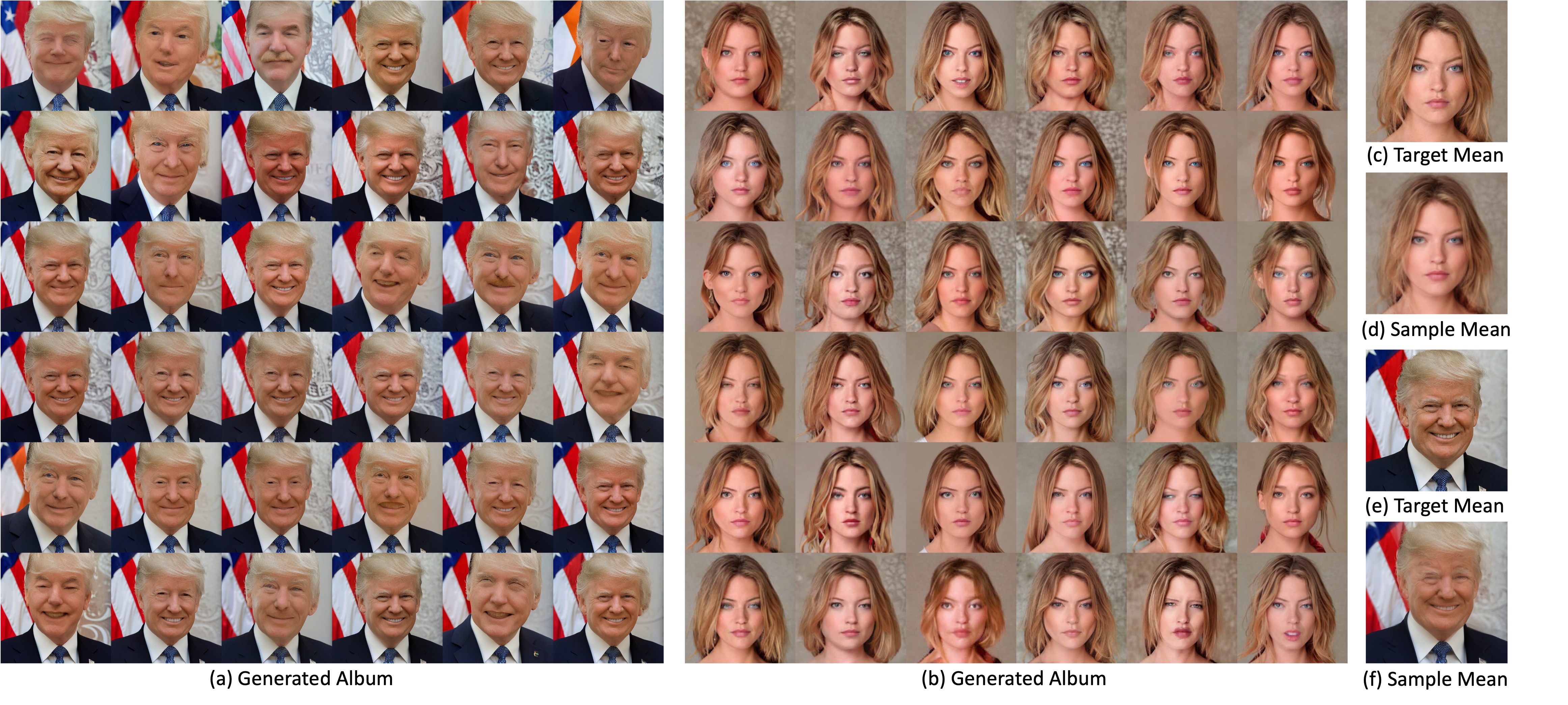
Figure 6: CCS-CT Sampled Images with Stable Diffusion 1.5. (a) Samples with an in-the-wild target mean (e) and a target rMSE 0.09; (b) Samples with a target mean (d) from Celeba-HQ dataset and a target rMSE 0.07; (d): sample mean from (a); (f): sample mean from (b).

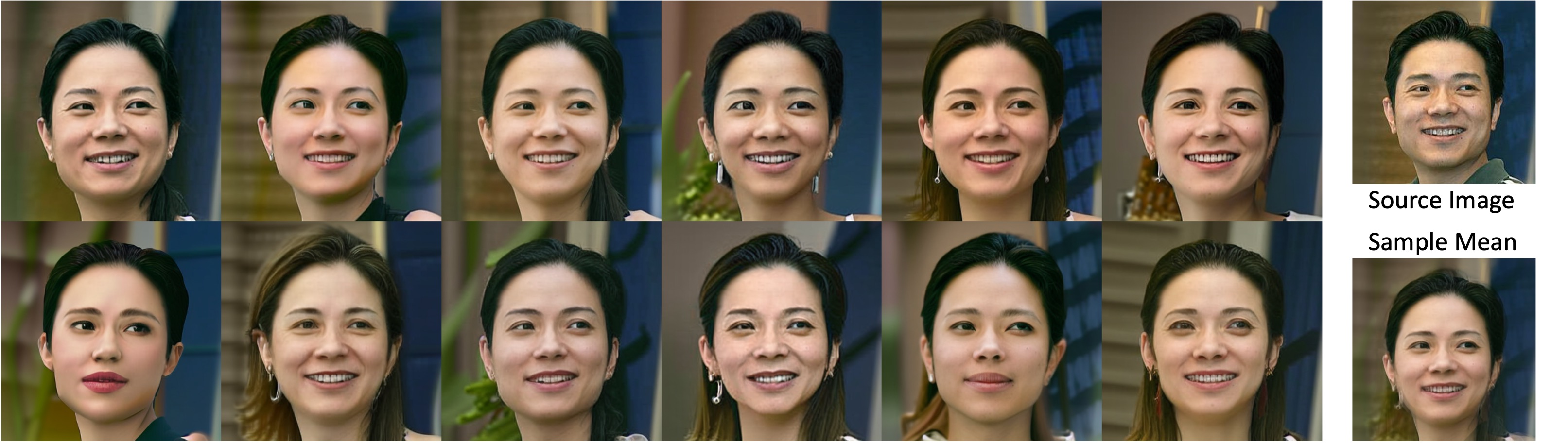
Figure 7: Image Editing Samples with Stable Diffusion 1.5, the source prompt is given by ‘a high-quality portrait of a man’, and the target prompt is given by ‘a high-quality portrait of a woman’, the target MSE level is given by 0.10

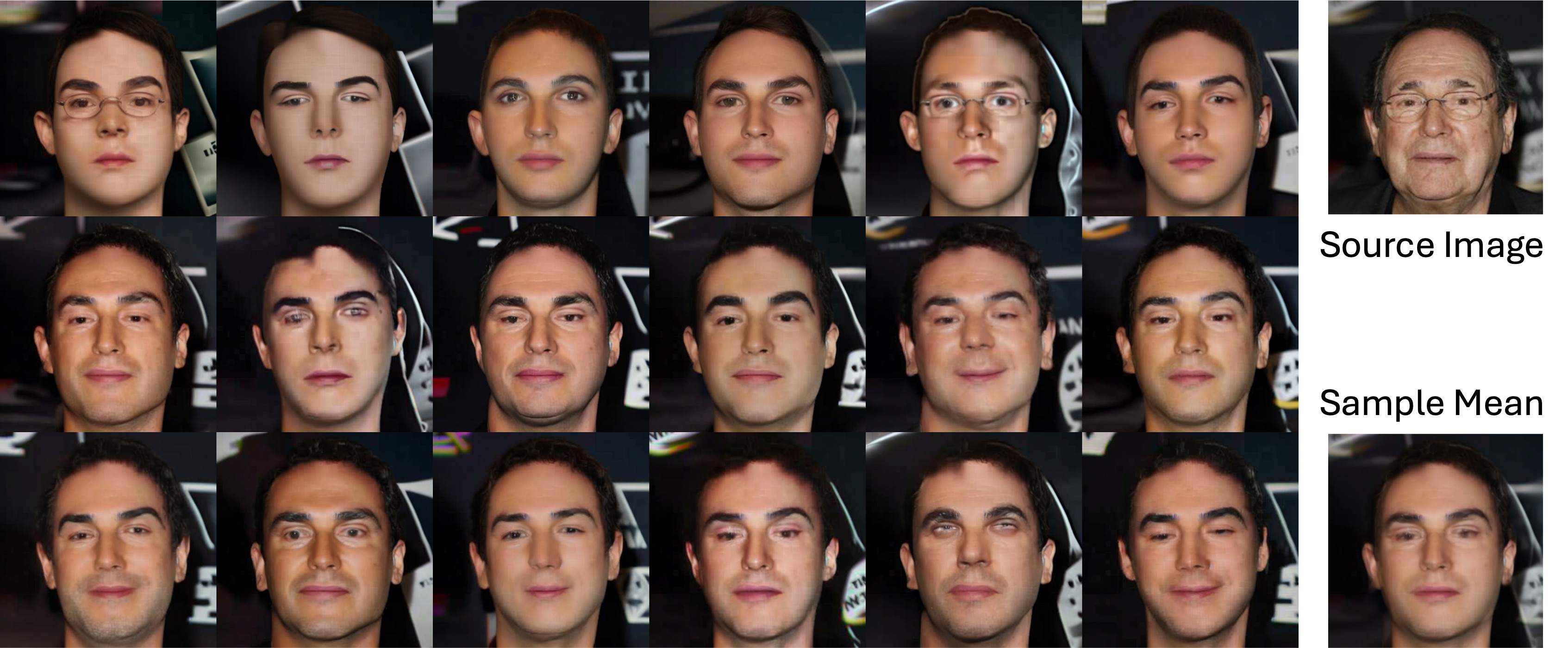
Figure 8: Image Editing Samples with Stable Diffusion 1.5, the source prompt is given by ‘a high-quality portrait of an old man’, and the target prompt is given by ‘a high-quality portrait of a young man’, the target MSE level is given by 0.09

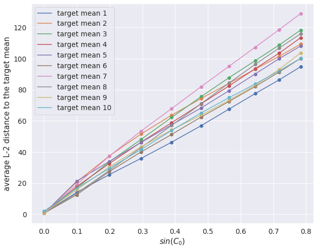
Figure 9: We first sample 50 images around each target mean in the FFHQ dataset. We then obtain the DDIM inverse of each target mean, and then add spherical perturbation to it. When the scale of perturbations $\sin(C_{0})$ increases, the average of norms of the residuals between each sample and the target mean approximately increases linearly.

References

- (1) Chen, S., Zhang, H., Guo, M., Lu, Y., Wang, P., and Qu, Q. Exploring low-dimensional subspace in diffusion models for controllable image editing. In The Thirty-eighth Annual Conference on Neural Information Processing Systems.
- Chen et al. (2024a) Chen, S., Kontonis, V., and Shah, K. Learning general gaussian mixtures with efficient score matching. arXiv preprint arXiv:2404.18893, 2024a.
- Chen et al. (2024b) Chen, S., Zhang, H., Guo, M., Lu, Y., Wang, P., and Qu, Q. Exploring low-dimensional subspace in diffusion models for controllable image editing. In The Thirty-eighth Annual Conference on Neural Information Processing Systems, 2024b. URL https://openreview.net/forum?id=50aOEfb2km.
- Choi et al. (2021) Choi, J., Kim, S., Jeong, Y., Gwon, Y., and Yoon, S. Ilvr: Conditioning method for denoising diffusion probabilistic models. In Proceedings of the IEEE/CVF International Conference on Computer Vision, pp. 14367–14376, 2021.
- Christie et al. (2018) Christie, G., Fendley, N., Wilson, J., and Mukherjee, R. Functional map of the world. In CVPR, 2018.
- (6) Chung, H., Kim, J., Mccann, M. T., Klasky, M. L., and Ye, J. C. Diffusion posterior sampling for general noisy inverse problems. In The Eleventh International Conference on Learning Representations.
- Chung et al. (2022a) Chung, H., Sim, B., Ryu, D., and Ye, J. C. Improving diffusion models for inverse problems using manifold constraints. Advances in Neural Information Processing Systems, 35:25683–25696, 2022a.
- Chung et al. (2022b) Chung, H., Sim, B., and Ye, J. C. Come-closer-diffuse-faster: Accelerating conditional diffusion models for inverse problems through stochastic contraction. In Proceedings of the IEEE/CVF Conference on Computer Vision and Pattern Recognition, pp. 12413–12422, 2022b.
- Chung et al. (2023) Chung, H., Ye, J. C., Milanfar, P., and Delbracio, M. Prompt-tuning latent diffusion models for inverse problems. arXiv preprint arXiv:2310.01110, 2023.
- Chung et al. (2024) Chung, J., Hyun, S., and Heo, J.-P. Style injection in diffusion: A training-free approach for adapting large-scale diffusion models for style transfer. In Proceedings of the IEEE/CVF Conference on Computer Vision and Pattern Recognition, pp. 8795–8805, 2024.
- De Bortoli (2022) De Bortoli, V. Convergence of denoising diffusion models under the manifold hypothesis. Transactions on Machine Learning Research, 2022.
- Dhariwal & Nichol (2021a) Dhariwal, P. and Nichol, A. Diffusion models beat gans on image synthesis. Advances in neural information processing systems, 34:8780–8794, 2021a.
- Dhariwal & Nichol (2021b) Dhariwal, P. and Nichol, A. Diffusion models beat GANs on image synthesis. Advances in neural information processing systems, 34:8780–8794, 2021b.
- Dwork (2006) Dwork, C. Differential privacy. In International colloquium on automata, languages, and programming, pp. 1–12. Springer, 2006.
- Epstein et al. (2023) Epstein, D., Jabri, A., Poole, B., Efros, A., and Holynski, A. Diffusion self-guidance for controllable image generation. Advances in Neural Information Processing Systems, 36:16222–16239, 2023.
- Gatmiry et al. (2024) Gatmiry, K., Kelner, J., and Lee, H. Learning mixtures of gaussians using diffusion models. arXiv preprint arXiv:2404.18869, 2024.
- Guo et al. (2024) Guo, X., Liu, J., Cui, M., Li, J., Yang, H., and Huang, D. Initno: Boosting text-to-image diffusion models via initial noise optimization. In Proceedings of the IEEE/CVF Conference on Computer Vision and Pattern Recognition, pp. 9380–9389, 2024.
- Hartman (2002) Hartman, P. Ordinary differential equations. SIAM, 2002.
- (19) He, Y., Murata, N., Lai, C.-H., Takida, Y., Uesaka, T., Kim, D., Liao, W.-H., Mitsufuji, Y., Kolter, J. Z., Salakhutdinov, R., et al. Manifold preserving guided diffusion. In The Twelfth International Conference on Learning Representations.
- Hong et al. (2024) Hong, S., Lee, K., Jeon, S. Y., Bae, H., and Chun, S. Y. On exact inversion of dpm-solvers. In Proceedings of the IEEE/CVF Conference on Computer Vision and Pattern Recognition, pp. 7069–7078, 2024.
- Karras (2019) Karras, T. A style-based generator architecture for generative adversarial networks. arXiv preprint arXiv:1812.04948, 2019.
- Ke et al. (2021) Ke, J., Wang, Q., Wang, Y., Milanfar, P., and Yang, F. Musiq: Multi-scale image quality transformer. In Proceedings of the IEEE/CVF international conference on computer vision, pp. 5148–5157, 2021.
- (23) Kong, Z., Ping, W., Huang, J., Zhao, K., and Catanzaro, B. Diffwave: A versatile diffusion model for audio synthesis. In International Conference on Learning Representations.
- Krizhevsky et al. (2009) Krizhevsky, A., Hinton, G., et al. Learning multiple layers of features from tiny images. 2009.
- Kwon & Ye (2024) Kwon, T. and Ye, J. C. Solving video inverse problems using image diffusion models. arXiv preprint arXiv:2409.02574, 2024.
- Liu et al. (2024) Liu, H., Xu, C., Yang, Y., Zeng, L., and He, S. Drag your noise: Interactive point-based editing via diffusion semantic propagation. In Proceedings of the IEEE/CVF Conference on Computer Vision and Pattern Recognition, pp. 6743–6752, 2024.
- Narasimhan et al. (2024) Narasimhan, S. S., Agarwal, S., Rout, L., Shakkottai, S., and Chinchali, S. P. Constrained posterior sampling: Time series generation with hard constraints. arXiv preprint arXiv:2410.12652, 2024.
- Nichol & Dhariwal (2021) Nichol, A. Q. and Dhariwal, P. Improved denoising diffusion probabilistic models. In International conference on machine learning, pp. 8162–8171. PMLR, 2021.
- Rombach et al. (2022) Rombach, R., Blattmann, A., Lorenz, D., Esser, P., and Ommer, B. High-resolution image synthesis with latent diffusion models. In Proceedings of the IEEE/CVF conference on computer vision and pattern recognition, pp. 10684–10695, 2022.
- Salimans et al. (2016) Salimans, T., Goodfellow, I., Zaremba, W., Cheung, V., Radford, A., and Chen, X. Improved techniques for training gans. Advances in neural information processing systems, 29, 2016.
- Shoemake (1985) Shoemake, K. Animating rotation with quaternion curves. In Proceedings of the 12th annual conference on Computer graphics and interactive techniques, pp. 245–254, 1985.
- (32) Song, B., Kwon, S. M., Zhang, Z., Hu, X., Qu, Q., and Shen, L. Solving inverse problems with latent diffusion models via hard data consistency. In The Twelfth International Conference on Learning Representations.
- Song et al. (2020) Song, J., Meng, C., and Ermon, S. Denoising diffusion implicit models. arXiv preprint arXiv:2010.02502, 2020.
- Song et al. (2021) Song, J., Meng, C., and Ermon, S. Denoising diffusion implicit models. In International Conference on Learning Representations, 2021. URL https://openreview.net/forum?id=St1giarCHLP.
- Song et al. (2023) Song, J., Zhang, Q., Yin, H., Mardani, M., Liu, M.-Y., Kautz, J., Chen, Y., and Vahdat, A. Loss-guided diffusion models for plug-and-play controllable generation. In International Conference on Machine Learning, pp. 32483–32498. PMLR, 2023.
- Song & Ermon (2019) Song, Y. and Ermon, S. Generative modeling by estimating gradients of the data distribution. Advances in neural information processing systems, 32, 2019.
- Wang et al. (2023) Wang, J., Chan, K. C., and Loy, C. C. Exploring clip for assessing the look and feel of images. In Proceedings of the AAAI Conference on Artificial Intelligence, volume 37, pp. 2555–2563, 2023.
- Wang et al. (2024) Wang, P., Zhang, H., Zhang, Z., Chen, S., Ma, Y., and Qu, Q. Diffusion models learn low-dimensional distributions via subspace clustering. arXiv preprint arXiv:2409.02426, 2024.
- Wu & De la Torre (2023) Wu, C. H. and De la Torre, F. A latent space of stochastic diffusion models for zero-shot image editing and guidance. In Proceedings of the IEEE/CVF International Conference on Computer Vision, pp. 7378–7387, 2023.
- Xia et al. (2021) Xia, W., Yang, Y., Xue, J.-H., and Wu, B. Tedigan: Text-guided diverse face image generation and manipulation. In IEEE Conference on Computer Vision and Pattern Recognition (CVPR), 2021.
- Zhang et al. (2023a) Zhang, J., Das, K., and Kumar, S. On the robustness of diffusion inversion in image manipulation. In ICLR 2023 Workshop on Trustworthy and Reliable Large-Scale Machine Learning Models, 2023a.
- Zhang et al. (2023b) Zhang, L., Rao, A., and Agrawala, M. Adding conditional control to text-to-image diffusion models. In Proceedings of the IEEE/CVF International Conference on Computer Vision, pp. 3836–3847, 2023b.
- Zheng et al. (2024) Zheng, P., Zhang, Y., Fang, Z., Liu, T., Lian, D., and Han, B. Noisediffusion: Correcting noise for image interpolation with diffusion models beyond spherical linear interpolation. In The Twelfth International Conference on Learning Representations, 2024.