Rethinking Oversmoothing in Graph Neural Networks:
A Rank-Based Perspective

Abstract

Oversmoothing is a fundamental challenge in graph neural networks (GNNs): as the number of layers increases, node embeddings become increasingly similar, and model performance drops sharply. Traditionally, oversmoothing has been quantified using metrics that measure the similarity of neighbouring node features, such as the Dirichlet energy. While these metrics are related to oversmoothing, we argue they have critical limitations and fail to reliably capture oversmoothing in realistic scenarios. For instance, they provide meaningful insights only for very deep networks and under somewhat strict conditions on the norm of network weights and feature representations. As an alternative, we propose measuring oversmoothing by examining the numerical or effective rank of the feature representations. We provide theoretical support for this approach, demonstrating that the numerical rank of feature representations converges to one for a broad family of nonlinear activation functions under the assumption of nonnegative trained weights. To the best of our knowledge, this is the first result that proves the occurrence of oversmoothing without assumptions on the boundedness of the weight matrices. Along with the theoretical findings, we provide extensive numerical evaluation across diverse graph architectures. Our results show that rank-based metrics consistently capture oversmoothing, whereas energy-based metrics often fail. Notably, we reveal that a significant drop in the rank aligns closely with performance degradation, even in scenarios where energy metrics remain unchanged.

1 Introduction

Graph neural networks (GNNs) have emerged as a powerful framework for learning representations from graph-structured data, with applications spanning knowledge retrieval and reasoning (Peng et al., 2023; Tian et al., 2022), personalised recommendation systems (Damianou et al., 2024; Peng et al., 2022), social network analysis (Fan et al., 2019), and 3D mesh classification (Shi & Rajkumar, 2020). Central to most GNN architectures is the message-passing paradigm, where node features are iteratively aggregated from their neighbours and transformed using learned functions, such as multi-layer perceptrons or graph-attention mechanisms.

However, the performance of message-passing-based GNNs is known to deteriorate after only a few layers, essentially placing a soft limit on the depth of GNNs. This is often linked to the observation of increasing similarity between learned features as GNNs deepen and is named oversmoothing (Li et al., 2018; Nt & Maehara, 2019).

Over the years, oversmoothing in GNNs, as well as methods to alleviate it, have been studied based on the decay of some node feature similarity metrics, such as the Dirichlet energy and its variants (Oono & Suzuki, 2019; Cai & Wang, 2020; Bodnar et al., 2022; Nguyen et al., 2022; Di Giovanni et al., 2023; Wu et al., 2023; Roth & Liebig, 2023). At a high level, most of these metrics directly measure the norm of the absolute deviation from the dominant eigenspace of the message-passing matrix. In linear GNNs without bias terms, this eigenspace is often known and easily computable via e.g. the power method. However, when nonlinear activation functions or biases are used, the dominant eigenspace may change, causing these oversmoothing metrics to fail and give false negative signals about the oversmoothing state of the learned features.

Therefore, these metrics are often considered as providing sufficient but not necessary evidence for oversmoothing (Rusch et al., 2023a). Despite this, there is a considerable body of literature using these somewhat unreliable metrics as part of their evidence for non-occurrence of oversmoothing in GNNs (Zhou et al., 2021; Chen et al., 2022; Rusch et al., 2022; Wang et al., 2022; Maskey et al., 2023; Nguyen et al., 2023; Rusch et al., 2023b; Epping et al., 2024; Scholkemper et al., 2024; Wang & Cho, 2024).

As we show in Section 6, the performance degradation of GNNs trained on real datasets often happens well before any noticeable decay in these oversmoothing metrics can be observed. Most empirical studies in the literature that observe the decay of the Dirichlet-energy-like metrics are conducted over the layers of the same very deep untrained (with randomly sampled weights) or effectively untrained GNNs (Rusch et al., 2022; Wang et al., 2022; Rusch et al., 2023b; Wu et al., 2023), where the decay of the metrics is likely driven by the small weight initializations reducing all features to zero. Instead, we observe that when GNNs of different depths are separately trained, these metrics do not correlate well with their performance degradation.

Furthermore, we note that these metrics can only indicate oversmoothing when their values converge exactly to zero, corresponding to either an exact alignment to the dominant eigenspace or to the feature representation matrix collapsing to the all-zero matrix. This double implication presents an issue: in realistic settings with a large but not excessively large number of layers, we may observe the decay of the oversmoothing metric by, say, two orders of magnitude while still being far from zero. In such cases, it is unclear whether the features are aligning with the dominant eigenspace, simply decreasing in magnitude, or exhibiting neither of the two behaviours. As a result, these types of metrics provide little to no explanation for the degradation of GNN performance.

As an alternative to address these shortcomings, we advocate for the use of a continuous approximation of the rank of the network’s feature representations to measure oversmoothing. Our experimental evaluation across various GNN architectures trained for node classification demonstrates that continuous rank relaxations, such as the numerical rank and the effective rank, correlate strongly with performance degradation in independently trained GNNs—even in settings where popular energy-like metrics show little to no correlation.

Overall, the main contributions of this paper are as follows:

• We review popular oversmoothing metrics in the current literature and provide a novel perspective on their theoretical analysis based on nonlinear activation eigenvectors.

• Based on this analysis and observations on the linear case, we propose the rank as a better metric for quantifying oversmoothing, and thereby re-defining oversmoothing in GNNs as the convergence towards a low-rank matrix rather than to a matrix of exactly rank one.

• We prove the convergence of the numerical rank towards one for linear GNNs and nonlinear GNNs where the eigenvector of the message-passing matrix is also the eigenvector of the nonlinear activation function under the assumption of non-negative weights. To our knowledge, this is the first theoretical result proving that oversmoothing may occur independently of the weights’ magnitude with nonlinear activation functions.

• We provide extensive numerical evidence that continuous rank relaxation functions better capture oversmoothing than commonly used Dirichlet-like metrics.

2 Background

2.1 Graph Convolutional Network

Let $\mathcal{G}=(\mathcal{V},\mathcal{E})$ be an undirected graph with $\mathcal{V}$ denoting its set of vertices and $\mathcal{E}\subseteq\mathcal{V}\times\mathcal{V}$ its set of edges. Let $\widetilde{A}\in\mathbb{R}^{N\times N}$ be the unweighted adjacency matrix with $N=|\mathcal{V}|$ being the total number of nodes, $|\mathcal{E}|$ being the total number of edges of $\mathcal{G}$ and $A$ the corresponding symmetric adjacency matrix normalized by the node degrees:

$$A=\widetilde{D}^{-1/2}\widetilde{A}\widetilde{D}^{-1/2},$$ (1)

where $\widetilde{D}=D+I$, $D$ is the diagonal degree matrix of the graph $\mathcal{G}$, and $I$ is the identity matrix. The rows of the feature matrix $X\in\mathbb{R}^{N\times d}$ are the concatenation of the $d$-dimensional feature vectors of all nodes in the graph. At each layer $l$, the GCN updates the node features as follows

$$X^{(l+1)}=\sigma(AX^{(l)}W^{(l)})$$ (2)

where $\sigma$ is a nonlinear activation function, applied componentwise, and $W^{(l)}$ is a trainable weight matrix.

2.2 Graph Attention Network

While GCNs use a fixed normalized adjacency matrix to perform graph convolutions at each layer, Graph Attention Networks (GATs) (Veličković et al., 2017; Brody et al., 2021) perform graph convolution through a layer-dependent message-passing matrix $A^{(l)}$ learned through an attention mechanism as follows

$$A^{(l)}_{ij}=\text{softmax}_{j}(\sigma_{a}(p_{1}^{(l)\top}W^{(l)\top}X_{i}+p_{2}^{(l)\top}W^{(l)\top}X_{j}))$$ (3)

where $p_{i}^{(l)}$ are learnable parameter vectors, $X_{i},X_{j}$ denote the feature of the $i$th and $j$th nodes respectively, the activation $\sigma_{a}$ is typically chosen to be LeakyReLU, and $\text{softmax}_{j}$ corresponds to the row-wise normalization

$$\text{softmax}_{j}(A_{ij})=\frac{\exp(A_{ij})}{\sum_{j^{\prime}}\exp(A_{ij^{\prime}})}.$$ (4)

The corresponding feature update is

$$X^{(l+1)}=\sigma(A^{(l)}X^{(l)}W^{(l)})\,.$$ (5)

3 Oversmoothing

Oversmoothing can be broadly understood as an increase in similarity between node features as inputs are propagated through an increasing number of message-passing layers, leading to a noticeable decline in GNN performance. However, the precise definition of this phenomenon varies across different sources. Some works define oversmoothing more rigorously as the alignment of all feature vectors with each other. This definition is motivated by the behaviour of a linear GCN:

$$X^{(l+1)}=A\cdots AX^{(0)}W^{(0)}\dots W^{(l)}.$$ (6)

Indeed if $\widetilde{A}$ is the adjacency matrix of a fully connected graph $\mathcal{G}$, $A$ will have a spectral radius equal to $1$ with multiplicity $1$, and $A^{l}$ will thus converge towards the eigenspace spanned by the dominant eigenvector. Precisely, we have

$$A^{l}\to uv^{\top}\quad\text{as}\quad l\rightarrow\infty,$$ (7)

where $Au=u$, and $A^{\top}v=v$, see e.g. (Tudisco et al., 2015).

As a consequence, if the product of the weight matrices $W^{(0)}\cdots W^{(l)}$ converges in the limit $l\rightarrow\infty$, then the features degenerate to a matrix having rank at most one, where all the features are aligned with the dominant eigenvector $u$. Mathematically, if we assume $u$ to be such that $\|u\|=1$, this alignment can be expressed by stating that the difference between the features and their projection onto $u$, given by $\|X^{(l)}-uu^{T}X^{(l)}\|$, converges to zero.

3.1 Existing Oversmoothing Metrics

Motivated by the discussion about the linear case, oversmoothing is thus quantified and analysed in terms of the convergence of some node similarity metrics towards zero. In particular, in most cases, it is measured exactly by the alignment of the features with the dominant eigenvector of the matrix $A$. The most prominent metric that has been used to quantify oversmoothing is the Dirichlet energy, which measures the norm of the difference between the degree-normalized neighbouring node features (Cai & Wang, 2020; Rusch et al., 2023a)

$$E_{\mathrm{Dir}}(X)=\sum_{(i,j)\in\mathcal{E}}\left\|\frac{X_{i}}{u_{i}}-\frac{X_{j}}{u_{j}}\right\|^{2}_{2},$$ (8)

where $u_{i}$ is the $i$-th entry of the dominant eigenvector of the message-passing matrix in (1). It thus immediately follows from our discussion on the linear setting that $E_{\mathrm{Dir}}(X^{(l)})$ converges to zero as $l\to\infty$ for a linear GCN with converging weights product $W^{(0)}\cdots W^{(l)}$. This intuition suggests that a similar behaviour may occur for “smooth-enough” nonlinearities.

In particular, in the case of a GCN, the dominant eigenvector $u$ is defined by $u_{i}=\sqrt{1+d_{i}}$ and (Cai & Wang, 2020) have proved that, using LeakyReLU activation functions $E_{\mathrm{Dir}}(X^{(l+1)})\leq s_{l}\bar{\lambda}E_{\mathrm{Dir}}(X^{(l)})$, where $s_{l}=\|W^{(l)}\|_{2}$ is the largest singular value of the weight matrix $W^{(l)}$, and $\bar{\lambda}=(1-\min_{i}\lambda_{i})^{2}$, where $\lambda_{i}\in(0,2]$ varies among the nonzero eigenvalues of the normalized graph Laplacian $\widetilde{\Delta}=I-A=I-\widetilde{D}^{-\frac{1}{2}}\widetilde{A}\widetilde{D}^{-\frac{1}{2}}$.

Similarly, in the case of GATs, the matrices $A_{i}$ are all row stochastic, meaning that $u_{i}=1$ for all $i$. In this case, in (Wu et al., 2023), it has been proved that whenever the product of the entry-wise absolute value of the weights is bounded, that is $\|\Pi_{k=1}^{\infty}|W^{(k)}|\|<\infty$, then the following variant of the Dirichlet energy decays to zero

$$E_{\mathrm{Proj}}(X)=\|X-\mathcal{P}X\|^{2}_{F}$$ (9)

where $\mathcal{P}=uu^{\top}$ is the projection matrix on the space spanned by the dominant eigenvector $u$ of the matrices $A^{(l)}$. In particular, this metric can be used only if the dominant eigenvector $u$ is the same for all $l$; this is, for example, the case with row stochastic matrices or when $A^{(l)}=A$ for all $l$.

3.2 A unifying perspective based on the eigenvectors of nonlinear activations

In the following discussion, we present a unified and more general perspective of the necessary conditions to have oversmoothing in the sense of the classical metrics, based on the eigenvectors of a nonlinear activation function. In the interest of space, longer proofs for this and the subsequent sections are moved to Appendix A.

Definition 3.1.

We say that a vector $u\in\mathbb{R}^{N}\setminus\{0\}$ is an eigenvector of the (nonlinear) activation function $\sigma:\mathbb{R}^{N}\to\mathbb{R}^{n}$ if for any $t\in\mathbb{R}\setminus\{0\}$, there exists $\mu_{t}$ such that $\sigma(tu)=\mu_{t}u$.

With this definition, we can now provide a unifying characterization of message-passing operators $A^{(l)}$ and activation functions $\sigma$ that guarantee the convergence of the Dirichlet-like energy metric $E_{\mathrm{Proj}}$ to zero for the feature representation sequence defined by $X^{(l+1)}=\sigma(A^{(l)}X^{(l)}W^{(l)})$. Specifically, Theorem 3.3 shows that this holds provided all matrices $A^{(l)}$ share a common dominant eigenvector $u$, which is also an eigenvector of $\sigma$.

This assumption recurs throughout our theoretical analysis, aligning with existing results in the literature. For example, (a) the proof by Cai & Wang (2020) applies to GCNs with LeakyReLU, where the dominant eigenvector of $A$ is nonnegative by the Perron-Frobenius theorem and, therefore, an eigenvector of LeakyReLU; and (b) the proof by Wu et al. (2023) holds for stochastic message-passing matrices $A^{(l)}$, which inherently share a common dominant eigenvector with constant entries, that is an eigenvector for any pointwise nonlinear activation function.

Lemma 3.2.

Let $X^{(l+1)}=\sigma(A^{(l)}X^{(l)}W^{(l)})$ be the $l$-th layer of a GNN. Assume that $A^{(l)}$ has a simple dominant eigenvalue with corresponding eigenvector $u$ that is also an eigenvector of $\sigma$. If $\sigma$ is $1$-Lipschitz, namely $\|\sigma(x)-\sigma(y)\|\leq\|x-y\|$ for any $x,y$, then

$$\|(I-\mathcal{P})X^{(l+1)}\|_{F}\leq\|(I-\mathcal{P})A^{(l)}X^{(l)}W^{(l)}\|_{F},$$

where $\mathcal{P}=uu^{T}/\|u\|^{2}$ is the projection matrix on the linear space spanned by $u$.

The following theorem follows as a consequence.

Theorem 3.3.

With the same notation of Lemma 3.2, if

$$\lim_{L\to\infty}\prod_{l=0}^{L}\|(I-\mathcal{P})A^{(l)}\|_{2}\|W^{(l)}\|_{2}=0,$$

then $E_{\mathrm{Proj}}(X^{(l)})\to 0$ as $l\to\infty$.

Proof.

The proof follows observing that in the decomposition $(I-\mathcal{P})A^{(l)}=(I-\mathcal{P})A^{(l)}\mathcal{P}+(I-\mathcal{P})A^{(l)}(I-\mathcal{P})$ the matrix $(I-\mathcal{P})A^{(l)}\mathcal{P}$ is zero because $A^{(l)}u=\lambda_{1}^{l}u$ for any $l$. Thus

$$(I-\mathcal{P})A^{(l)}=(I-\mathcal{P})A^{(l)}(I-\mathcal{P}),$$

and, from Lemma 3.2 and the inequality $\|AB\|_{F}\leq\|A\|_{2}\|B\|_{F}$, we have $\|(I-\mathcal{P})X^{(L)}\|_{F}\leq\Big{(}\Pi_{l=0}^{L-1}\|(I-\mathcal{P})A^{(l)}\|_{2}\|W^{(l)}\|_{2}\Big{)}\|X^{(0)}\|_{F}$. ∎

Note, in particular, that in the case of GCNs, the matrix $A^{(l)}=A$ is symmetric, and thus $\|I-\mathcal{P}A^{(l)}\|_{2}=\lambda_{2}$. Therefore, when $\sigma=\text{LeakyReLU}$, we obtain the result by Cai & Wang (2020) as convergence to zero is guaranteed if $\|W^{(l)}\|_{2}\leq\lambda_{2}$. Recall that, as discussed above, the choice $\sigma=\text{LeakyReLU}$ satisfies our eigenvector assumption since $u\geq 0$ by the Perron-Frobenius theorem, and thus LeakyReLU$(tu)=\alpha tu$ with $\alpha$ depending only on the sign of $t$. Similarly, in the case of GATs, the matrices $A^{(l)}$ are stochastic for all $l$, implying that $u=\mathbbm{1}$ is the constant vector with $(u)_{i}=1$ for all $i$. If $\sigma=\otimes\psi$ is a nonlinear activation function acting entrywise through $\psi$, then $\sigma(t\mathbbm{1})=\psi(t)\mathbbm{1}$. Therefore, Theorem 3.3 implies that if the weights are sufficiently small, the features align independently of the activation function used. This is consistent with the results in (Wu et al., 2023). However, we note that the bounds on the weights required by Theorem 3.3 and those in (Wu et al., 2023) on the weights $W^{(l)}$ are not identical, and it is unclear which of the two is more significant. Nonetheless, in both cases, having bounded weights along with any $1$-Lipschitz pointwise activation function is a sufficient condition for observing oversmoothing via $E_{\mathrm{Proj}}$ in GATs. In addition to offering a different and unifying theoretical perspective on the results in (Cai & Wang, 2020; Wu et al., 2023), we highlight the simplicity of our eigenvector-based proof, which we hope provides added clarity on this phenomenon.

4 Energy-like metrics: what can go wrong

Energy-like metrics such as $E_{\mathrm{Dir}}$ and $E_{\mathrm{Proj}}$ are among the most commonly used oversmoothing metrics. However, they suffer from inherent limitations that hinder their practical usability and informational content.

One important limitation of these metrics is that they indicate oversmoothing only in the limit of infinitely many layers, when their values converge exactly to zero. Since they measure a form of absolute distance, a small but nonzero value does not provide any meaningful information. On the other hand, convergence to zero corresponds to either perfect alignment with the dominant eigenspace or the collapse of the feature representation matrix to the all-zero matrix. While the former is a symptom of oversmoothing, the latter does not necessarily imply oversmoothing. Moreover, this convergence property requires the weights to be bounded. However, in practical cases, performance degradation is observed even in relatively shallow networks, far from being infinitely deep, and with arbitrarily large (or small) weight magnitudes. This aligns with our intuition and what occurs in the linear case. Indeed, for a linear GCN, even when the features $X^{(l)}$ grow to infinity as $l\to\infty$, one observes that $X^{(l)}$ becomes dominated by the dominant eigenspace of $A$, even for finite and possibly small values of $l$, depending on the spectral gap of the graph.

More precisely, the following theorem holds:

Theorem 4.1.

Let $X^{(l+1)}=AX^{(l)}W^{(l)}$ be a linear GCN. Let $\lambda_{1},\lambda_{2}$ be the largest and second-largest eigenvalues (in modulus) of $A$, respectively. Assume the weights $\{W^{(l)}\}_{l=1}^{\infty}$ are randomly sampled from i.i.d. random variables with distribution $\nu$ such that

$$\int\log^{+}(\|W\|)d\nu+\int\log^{+}(\|W^{-1}\|)d\nu<\infty$$

with $\log^{+}(t)=\max\{\log(t),\,0\}$. If $|\lambda_{2}/\lambda_{1}|<1$, then almost surely, it holds that

$$\lim_{l\to\infty}\frac{\|(I-\mathcal{P})X^{(l)}\|_{F}}{\|\mathcal{P}X^{(l)}\|_{F}}=0$$

with a linear rate of convergence $O(|\lambda_{2}/\lambda_{1}|^{l})$.

In particular, the theorem above implies that for a large spectral gap $|\lambda_{2}/\lambda_{1}|\ll 1$, $X^{(l)}$ is predominantly of rank one, namely

$$X^{(l)}=\lambda_{1}^{l}\Big{(}uv^{T}+R(l)\Big{)}$$

for some $v$, with $R(l)\sim O(|\lambda_{2}/\lambda_{1}|)^{l}$ and thus converging to $0$ as $l\to\infty$. This results in weakly expressive feature representations, independently of the magnitude of the feature weights. This phenomenon can be effectively captured by measuring the rank of $X^{(l)}$, whereas Dirichlet-like energy measures may fail to detect it.

Another important limitation of these metrics is their dependence on a specific, known dominant eigenspace, which must either be explicitly known or computed in advance. Consequently, their applicability is strongly tied to the specific architecture of the network. In particular, the dominant eigenvector $u$ of $A^{(l)}$ must be known and remain the same for all $l$. This requirement excludes their use in most cases where $A^{(l)}$ varies with $l$, such as when $A^{(l)}$ is the standard weighted adjacency matrix of the graph.

5 The Rank as a Measure of Oversmoothing

Inspired by the behaviour observed in the linear case, we argue that measuring the rank of feature representations provides a more effective way to quantify oversmoothing, in alignment with recent work on oversmoothing (Guo et al., 2023). However, since the rank of a matrix is defined as the number of nonzero singular values, it is a discrete function and thus not suitable as a measure. A viable alternative is to use a continuous relaxation that closely approximates the rank itself.

Examples of possible continuous approximations of the rank include the numerical rank, the stable rank, and the effective rank (Roy & Vetterli, 2007; Rudelson & Vershynin, 2006; Arora et al., 2019). The stable rank is defined as $\text{StableRank}(X)=\|X\|_{*}^{2}/\|X\|_{F}^{2}$, where $\|X\|_{*}=\sum_{i}\sigma_{i}$ is the nuclear norm. The numerical rank is given by $\text{NumRank}(X)=\|X\|_{F}^{2}/\|X\|_{2}^{2}$. Finally, given the singular values $\sigma_{1}>\sigma_{2}>\dots>\sigma_{\min\{N,d\}}$ of $X$, the effective rank is defined as

$$\text{Erank}(X)=\exp\left(-\textstyle{\sum_{k}p_{k}\log p_{k}}\right),$$ (10)

where $p_{k}=\sigma_{k}/\sum_{i}\sigma_{i}$ is the $k$-th normalized singular value. These rank relaxation measures exhibit similar empirical behaviour as shown by our numerical evaluation in Section 6.

In practice, measuring oversmoothing in terms of a continuous approximation of the rank is a reasonable approach that helps address the limitations of Dirichlet-like measures. Specifically, it offers the following advantages: (a) it is scale-invariant, meaning it remains informative even when the feature matrix converges to zero or explodes to infinity; (b) it does not rely on a fixed, predetermined eigenspace but instead captures convergence of the feature matrix toward an arbitrary lower-dimensional subspace; (c) it allows for the detection of oversmoothing in shallow networks without requiring exact convergence to rank one—since a small value of, say, the effective rank, directly implies that the feature representations are low-rank, which in turn suggests a potentially suboptimal network architecture.

In Table 1, we present a toy example illustrating that classical oversmoothing metrics fail to correctly capture oversmoothing unless the features are perfectly aligned. This observation implies that these metrics can quantify oversmoothing only when the rank of the feature matrix converges exactly to one. In contrast, continuous rank functions provide a more reliable measure of approximate feature alignment. Later, in Figure 1, we demonstrate that the same phenomenon occurs in GNNs trained on real datasets, where exact feature alignment is rare. In such cases, classical metrics remain roughly constant, whereas the rank decreases, coinciding with a sharp drop in GNN accuracy.

Table 1: A set of toy scenarios depicting the behaviour of oversmoothing metrics. Each plot contains 50 nodes, each with two features plotted as the x and y axis. # 1: all features are of the same value; # 2: all features are assumed to align with the same vector exactly; # 3: shifts one (red) point in # 2 in y-direction; # 4: samples all points from a uniform distribution. MAD (see Section 6) and $E_{\mathrm{Dir}}$ give false negative signals in # 3 while the features are considered oversmoothing by definition. $E_{\mathrm{Proj}}$ can hardly differentiate between # 3 and # 4, and is thus not robust in quantifying oversmoothing. To compute $E_{\mathrm{Proj}}$ and $E_{\mathrm{Dir}}$ the first feature was considered in place of $u$ in (8) and (9).

	# 1	# 2	# 3	# 4
$E_{\mathrm{Dir}}$	0	0	13.25	77.78
$E_{\mathrm{Proj}}$	0	0	0.83	0.97
MAD	0	0.81	0.81	0.57
NumRank	1	1	1.01	1.78
Erank	1	1	1.36	1.99

5.1 Theoretical Analysis of Rank Decay

In this section, we provide an analytical study proving the decrease of the numerical rank for a broad class of graph neural network architectures under the assumption that the weight matrices are entrywise nonnegative. While this is a somewhat restrictive setting, our result is the first theoretical proof that oversmoothing occurs independently of the weight (and thus feature) magnitude.

We begin with several useful observations. Let $u$ be the dominant eigenvector of $A$ corresponding to $\lambda_{1}$ and satisfying $\|u\|=1$. Consider the projection matrix $\mathcal{P}=uu^{\top}$. Given a matrix $X$, we can decompose it as $X=\mathcal{P}X+(I-\mathcal{P})X$. Since $u$ is a unit vector, it follows that $\|\mathcal{P}\|_{2}=1$, and therefore,

$$\|X\|_{2}=\|\mathcal{P}\|_{2}\|X\|_{2}\geq\|\mathcal{P}X\|_{2}.$$ (11)

Moreover, since $\mathcal{P}X$ and $(I-\mathcal{P})X$ are orthogonal with respect to the Frobenius inner product, we have $\|\mathcal{P}X+(I-\mathcal{P})X\|_{F}^{2}=\|\mathcal{P}X\|_{F}^{2}+\|(I-\mathcal{P})X\|_{F}^{2}$. Thus, we obtain the following bound for the numerical rank of $X$:

$$\text{NumRank}(X) =\frac{\|\mathcal{P}X+(I-\mathcal{P})X\|_{F}^{2}}{\|X\|_{2}^{2}}$$ (12)

$$=\frac{\|\mathcal{P}X\|_{F}^{2}+\|(I-\mathcal{P})X\|_{F}^{2}}{\|X\|_{2}^{2}}$$

$$\leq 1+\frac{\|(I-\mathcal{P})X\|_{F}^{2}}{\|X\|_{2}^{2}},$$

where we used (11) and the fact that $\|\mathcal{P}X\|_{F}=\|\mathcal{P}X\|_{2}$ since $\mathcal{P}X$ is a rank-one matrix.

The above inequality, together with Theorem 4.1, allows us to establish the convergence of the numerical rank for linear networks.

The Linear Case

Consider a linear GCN of the form $X^{(l+1)}=AX^{(l)}W^{(l)}$, where $A$ has a simple dominant eigenvalue $\lambda_{1}$ satisfying $|\lambda_{1}|\geq|\lambda_{2}|$.

We have already noted that $\|X\|_{2}\geq\|\mathcal{P}X\|_{2}$, meaning that the numerical rank converges to one if $\|(I-\mathcal{P})X\|_{F}/\|X\|_{2}$ decays to zero. This occurs whenever the features grow faster in the direction of the dominant eigenvector than in any other direction. As established in Theorem 4.1, this is almost surely the case in linear GNNs. As a direct consequence, we obtain the following result:

Theorem 5.1.

Let $X^{(l+1)}=AX^{(l)}W^{(l)}$ be a linear GCN. Under the same assumptions as in Theorem 4.1, the following identity holds almost surely:

$$\lim_{l\rightarrow\infty}\mathrm{NumRank}(X^{(l)})=1.$$

Extending the result above to general GNNs with nonlinear activation functions is highly nontrivial. In the next section, we present our main theoretical result, which generalizes this analysis to a broader class of GNNs under the assumption of nonnegative weights.

5.2 The Nonnegative Setting

To study the case of networks with nonnegative weights, we make use of tools from the nonlinear Perron-Frobenius theory; we refer to (Lemmens & Nussbaum, 2012; Gautier et al., 2023) and the reference therein for further details.

We assume all the intermediate features to be in the positive open cone $\mathcal{K}:=\mathbb{R}_{+}^{N}=\{x\in\mathbb{R}^{N}\>|\>x_{i}>0\;\forall i=1,\dots,N\}$. On $\mathcal{K}$, it is possible to introduce the partial ordering

$$x\leq_{\mathcal{K}}y\>(x\ll_{\mathcal{K}}y)\quad\text{iff}\quad y-x\in\bar{\mathcal{K}}\>(y-x\in\mathcal{K})$$ (13)

where $\bar{\mathcal{K}}$ denotes the nonnegative closed cone. Given two points $x,y\in\mathcal{K}$ we write $M(x/y)=\max_{i}x_{i}/y_{i}$ and $m(x/y)=\min_{i}x_{i}/y_{i}$. Then, we can define the following Hilbert distance between any two points $x,y\in\mathcal{K}$,

$$d_{H}(x,y)=\log(M(x/y)/m(x/y)).$$

Note that $d_{H}$ is not a distance on $\mathcal{K}$, indeed $d_{H}(\alpha x,\beta y)=d_{H}(x,y)$ for any $x,y\in\mathcal{K}$ and $\alpha,\beta>0$. However it is a distance up to scaling; that is, it becomes a concrete distance whenever we restrict ourselves to a slice of the cone.

Now, it is well-known that any matrix $A$ such that $Ax\in\mathcal{K}$ for any $x\in\mathcal{K}$ is non-expansive with respect to the Hilbert distance, i.e.

$$d_{H}(Ax,Ay)\leq\beta d_{H}(x,y)\qquad\forall x,y\in\mathcal{K}$$ (14)

with $0\leq\beta\leq 1$. The last inequality is a consequence of the fact that $A$ preserves the ordering induced by the cone, i.e. if $x\geq_{\mathcal{K}}y$, then $Ax\geq_{\mathcal{K}}Ay$. In particular, we recall that (14) always hold for $\beta<1$ when $A$ is entry-wise strictly positive, as positive matrices map the whole $\bar{\mathcal{K}}$ in its interior, i.e. $x\geq_{\mathcal{K}}y$ implies $Ax>Ay$. In the next definition, we include all the nonnegative matrices that have the same behaviour as the positive matrices but only on a neighbourhood of a positive vector in $\mathcal{K}$.

Recall that any irreducible nonnegative matrix $A$ has a positive eigenvector $u$ corresponding to its dominant eigenvalue.

Definition 5.2.

A family of nonnegative irreducible matrices (possibly one single matrix) $\{A^{(l)}\}$ with the same dominant eigenvector $u>0$ is uniformly contractive with respect to $u$ if for any $C>0$ there exists some $\beta_{C}<1$ such that $d_{H}(A^{(l)}x,u)\leq\beta_{C}d_{H}(x,u)$ for all $l$ and $x\in\mathcal{K}$ such that $d_{H}(x,u)\leq C$.

The above definition is significantly weaker than asking for $A$ to be strictly positive. We show this with an illustrative example in Section A.3.

Consider now first the case of a linear function that can be represented in the form

$$F(X)=AXW,$$ (15)

where $X$ is a positive $N\times d$ matrix, $A$ and $W$ are nonnegative $N\times N$ and $d\times d$ matrices, respectively. Then, under mild assumptions, we can prove that the columns of $F(X)$ are closer to the dominant eigenvector $u$ of $A$ as compared to the columns of $X$.

Lemma 5.3.

Let $F(X)=AXW$ with $A$ nonnegative and irreducible with dominant eigenvector $u\in\mathcal{K}$. Assume also $X$ to be striclty positve and $W$ nonnegative with $\min_{j}\max_{i}W_{ij}>0$. If $A$ is contractive with respect to $u$ and $C=\max_{i}d_{H}(X_{i},u)$ then

$$\max_{i}d_{H}(F(X)_{i},u)\leq\beta_{C}\max_{i}d_{H}(X_{i},u),$$

where $Y_{i}$ denotes the $i$-th column of $Y$, and $\beta_{C}\leq 1$.

Nonlinear Perron-Frobenius theory extends some of the results about nonnegative matrices to particular classes of nonlinear functions. A function $\sigma\in C(\mathcal{K},\mathcal{K})$ is order preserving if given any $x,y\in\mathcal{K}$ with $x\geq_{\mathcal{K}}y$ then $\sigma(x)\geq_{\mathcal{K}}\sigma(y)$. Moreover $\sigma$ is subhomogenenous if $\sigma(\lambda x)\leq_{\mathcal{K}}\lambda\sigma(x)$ for all $x\in\mathcal{K}$ and any $\lambda>1$. In particular, it is strictly subhomogeneous if $\sigma(\lambda x)\ll_{\mathcal{K}}\lambda\sigma(x)$ for all $x\in\mathcal{K}$ and $\lambda>1$ and homogeneous if $\sigma(\lambda x)=\lambda\sigma(x)$ for all $x\in\mathcal{K}$ and $\lambda\geq 0$ .

Subohomogeneity is a useful property and of practical utility. In fact, as discussed in, e.g. (Sittoni & Tudisco, 2024; Piotrowski et al., 2024), it is not difficult to verify that a broad range of activation functions commonly used in deep learning is subhomogeneous on $\mathcal{K}$. For this family of activation functions, Lemma 5.3 combined with arguments from nonlinear Perron–Frobenius theory yield the following main result

Theorem 5.4.

Consider a positive GNN

$$X^{(l+1)}=\sigma(A^{(l)}X^{(l)}W^{(l)})$$ (16)

with $X^{(0)}_{i}\in\mathcal{K}$ for any $i=1,\dots,d$ and $A^{(l)}$ and $W^{(l)}$ nonnegative for any $l$. Assume also that $u\in\mathcal{K}$ is the dominant eigenvector of all of the matrices $A^{(i)}$ and that it is also an eigenvector of $\sigma$. Then, if the matrices $\{A^{(i)}\}$ are uniformly contractive with respect to $u$ and $\min_{j}\max_{i}{W^{(l)}}_{ij}>0$ for any $l$, it holds

$$\lim_{l\rightarrow\infty}\mathrm{NumRank}(X^{(l)})=1.$$

We conclude with a formal investigation of the eigenpairs of activation functions that are entrywise subhomogeneous. Let $\sigma=\otimes^{N}\psi$ with $\psi\in C(\mathbb{R},\mathbb{R})$ that is subhomogeneous on $\mathbb{R}_{+}$. Then one can easily show that $\sigma$ is itself subhomogeneous on $\mathbb{R}^{N}_{+}$. We have,

Proposition 5.5.

Let $\sigma=\otimes^{N}\psi$ with $\psi\in C(\mathbb{R}_{+},\mathbb{R}_{+})$ be order preserving. Then: 1) If $\sigma$ is homogeneous, any positive vector is an eigenvector of $\sigma$. 2) If $\sigma$ is strictly subhomogeneous, the only eigenvector of $\sigma$ in $\mathcal{K}$ is the constant vector.

As a consequence of the above result, we find that the numerical rank of the features collapses both for GCNs with LeakyReLU activation function (that is homogeneous) as well as for GATs with any kind of subhomogeneous activation function. In fact, the constant vector is always an eigenvector of an entriwise nonlinear map.

Table 2: The table lists the correlation coefficients of logarithm of metric values and the classification accuracies for GNNs of depth 2 - 24 layers and separately trained on Cora dataset. For Erank and NumRank, we subtract 1 so that both metrics converge to zero. The classification accuracy ratio are computed on 2-layered and 24-layered GNNs.

Architecture	$E_{\mathrm{Dir}}$		$E_{\mathrm{Proj}}$		MAD	Erank	NumRank	Accuracy ratio
	Standard	Normalized	Standard	Normalized
LReLU + GCN	-0.7871	0.6644	-0.8106	-0.8309	-0.2460	0.9724	0.5885	0.2689
Tanh + GCN	0.5243	0.9403	0.8610	0.9768	0.9734	0.9923	0.9784	0.1937
LReLU + GCN + Bias	-0.9300	0.7505	-0.9414	-0.3642	-0.2828	0.9847	0.7833	0.2108
Tanh + GCN + Bias	0.4086	0.8950	0.7479	0.9026	0.8996	0.9926	0.9814	0.2133
LReLU + GCN + LayerNorm	-0.9132	0.8445	-0.9424	0.5591	0.9753	0.9736	0.9736	0.4882
Tanh + GCN + LayerNorm	-0.7119	0.2560	-0.2069	0.9716	0.8695	0.9576	0.9684	0.1885
LReLU + GCN + PairNorm	-0.8165	0.3731	-0.8106	0.3885	0.4850	0.5597	0.6244	0.8252
Tanh + GCN + PairNorm	-0.5963	0.0346	-0.5401	-0.3358	-0.0631	0.9838	0.9298	0.2902
LReLU + GAT	-0.9189	0.6703	-0.9469	-0.6054	0.8251	0.9722	0.7612	0.2487
Tanh + GAT	0.8300	0.8501	0.8676	0.9066	0.8603	0.9600	0.9515	0.1767
Average correlation	-0.3911	0.6279	-0.2722	0.2568	0.5296	0.9349	0.8541

6 Experiments

Empirical studies on the evolution of oversmoothing measures often use untrained, hundred-layer-deep GNNs (Rusch et al., 2022; Wang et al., 2022; Rusch et al., 2023b; Wu et al., 2023). We emphasize that this is an overly simplified setting. In more realistic settings, as the ones considered in this section, a trained GNN may suffer from significant performance degradation after only few-layers, at which stage the convergence patterns of most of the metrics are difficult to observe. The experiments that we present in this section validate the robustness of the effective rank and numerical rank in quantifying oversmoothing in GNNs against the other metrics.

In particular, we compare how different overmoothing metrics behave compared to the classification accuracy, varying the GNN architectures for node classification on real-world graph data. In our experiments, we consider the following metrics:

• The Dirichlet Energy $E_{\mathrm{Dir}}$ (Cai & Wang, 2020; Rusch et al., 2023a) and its variant $E_{\mathrm{Proj}}$ (Wu et al., 2023). Both are discussed in Section 3.1, see in particular (8) and (9).

• Normalized versions of the Dirichlet energy and its variant, namely $E_{\mathrm{Dir}}(X)/\|X\|_{F}^{2}$ and $E_{\mathrm{Proj}}(X)/\|X\|_{F}$. Indeed, from our previous discussion, a robust oversmoothing measure should be scale invariant with respect to the features. Metrics with global normalization like the ones we consider here have also been proposed in (Di Giovanni et al., 2023; Roth & Liebig, 2023; Maskey et al., 2023).

• The Mean Average Distance (MAD) (Chen et al., 2020)

  $$\text{MAD}(X)=\frac{1}{|\mathcal{E}|}\sum_{(i,j)\in\mathcal{E}}\left(1-\frac{X_{i}^{\top}X_{j}}{|X_{i}||X_{j}|}\right).$$ (17)

  It measures the cosine similarity between the neighbouring nodes. Unlike previous baselines, this oversmoothing metric does not take into account the dominant eigenvector of the matrices $A^{(l)}$.

• Relaxed rank metrics: We consider the Numerical Rank and Effective Rank. Both are discussed in Section 5. We point out that from our theoretical investigation, in particular from (12), the numerical rank decays to $1$ faster than the decay of the normalized $E_{\mathrm{Proj}}$ energy to zero. This further supports the use of the Numerical Rank as an improved measure of oversmoothing with respect to $E_{\mathrm{Proj}}$.

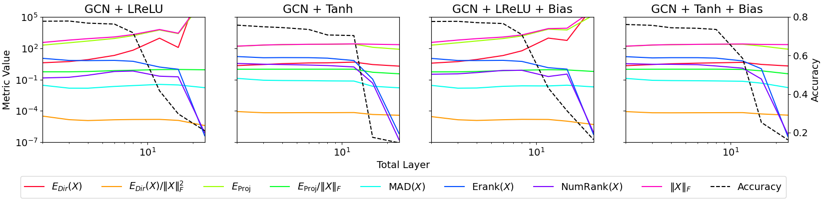
Figure 1: Four examples of GCNs corresponding to the first fours rows in table 2. For Erank and Numrank, we measure Erank$(X)-r^{*}_{\mathrm{ER}}$ and $\mathrm{NumRank}(X)-r^{*}_{\mathrm{NR}}$ for some $r^{*}>1$. In these particular cases, $r^{*}_{\mathrm{ER}}<1.85$, $r^{*}_{\mathrm{NR}}<1.3$. Note that the effective rank and numerical rank of the input features $X^{(0)}$ is about 1084 and 13.6, respectively.

In Table 2 and Figure 1, we train GNNs of a fixed hidden dimension equal to 32 on the Cora dataset. More results on Cora, as well as other datasets, are reported in Appendix B. We follow the standard setups of GCN and GAT as stated in equation (2) and (5), and use homogeneous LeakyReLU (LReLU) and subhomogenous Tanh as activation functions. For the GCN model, we also consider adding additional components, i.e. bias, LayerNorm (Ba et al., 2016) and PairNorm (Zhao & Akoglu, 2019). For each configuration, GNNs of eight different depths ranging from 2 to 24 are trained. The oversmoothing metric and accuracy results are averaged over 10 separately trained GNNs. All GNNs are trained with NAdam Optimizer and a constant learning rate of 0.01. The oversmoothing metrics are computed at the last hidden layer before the output layer. In Figure 1 and in Appendix B, we plot the behaviour of the different oversmoothing measures as well as the norm of the features and the accuracy of the trained GNNs when the depth of the network is increased. These figures clearly show that the network suffers a significant drop in accuracy, which is not matched by any visible change in standard oversmoothing metrics. By contrast, the rank of the feature representations decreases drastically, following quite closely the behaviour of the network’s accuracy. These findings are further sustained by the results shown in Table 2, where we compute the Pearson correlation coefficient between the logarithm of every measure and the classification accuracy of every GNN model. The use of a logarithmic transformation is based on the understanding that oversmoothing grows exponentially with the length of the network.

7 Conclusion

In this paper, we have discussed the problem of quantifying oversmoothing in GNNs. After discussing the limitations of the leading oversmoothing measures, we have proposed the use of the rank of the features as a better measure of oversmoothing. The experiments that we provided validate the robustness of the effective rank against the classical measures. In addition, we have proved theoretically the decay of the rank of the features for linear and nonnegative GNNs.

Appendix A Proofs of the main results

A.1 proof of Lemma 3.2

Let $\pi:=\mathrm{span}\{uv^{T}\,|\;v\in\mathbb{R}^{d}\}$ be the $1$-dimensional matrix subspace of the rank-$1$ matrices having columns aligned to $u$. Then it is easy to note that given some matrix $X$, $(I-\mathcal{P})X$ provides the projection of the matrix $X$ on the subspace $\pi$, i.e.

$$(I-\mathcal{P})X=\mathrm{proj}_{\pi}(X).$$ (18)

Indeed $\langle(I-\mathcal{P})X,uv^{T}\rangle_{F}=\mathrm{Tr}(vu^{T}(I-uu^{T})X)=0$. In particular, since the projection realizes the minimal distance, we have that

$$\|X-\mathcal{P}X\|_{F}\leq\|X-uv^{T}\|_{F}\qquad\forall v\in\mathbb{R}^{d}.$$ (19)

Now observe that $\sigma(uu^{T}A^{(l-1)}X^{(l-1)}W^{(l-1)})=u\bar{v}^{T}$ for some $\bar{v}$. Indeed, writing $v^{T}=u^{T}A^{(l-1)}X^{(l-1)}W^{(l-1)}$, we have that the $i$-th column of $\sigma(uu^{T}A^{(l-1)}X^{(l-1)}W^{(l-1)})$ is equal to $\sigma(v_{i}u)=\bar{v}_{i}u$ for some $\bar{v}_{i}$, because $u$ is an eigenvector of $\sigma$. As a consequence we have

$$\|(I-\mathcal{P})X^{(l)}\|_{F} \leq\|X^{(l)}-\sigma(uu^{T}A^{(l-1)}X^{(l-1)}W^{(l-1)})\|_{F}$$ (20)

$$=\|\sigma(A^{(l-1)}X^{(l-1)}W^{(l-1)})-\sigma(uu^{T}A^{(l-1)}X^{(l-1)}W^{(l-1)})\|_{F}$$

$$\leq\|(I-\mathcal{P})A^{(l-1)}X^{(l-1)}W^{(l-1)}\|_{F}$$

where we have used the $1$-Lipschitz property of $\sigma$.

A.2 Proof for Theorem 4.1

Start by studying the norm of $(I-\mathcal{P})X^{(l)}$. Then looking at the shape of the powers of the Jordan blocks matrix it is not difficult to note that $\widetilde{T}^{l}=O({l\choose N}\lambda_{2}^{l-N})$ for $l$ larger than $N$. In particular if we look at the explicit expression of $(I-\mathcal{P})X^{(l)}$

$$(I-P)X^{(l)}=\begin{pmatrix}0&(I-\mathcal{P})\tilde{M}\end{pmatrix}\begin{pmatrix}0&0\\ 0&\tilde{T}^{l}\end{pmatrix}M^{-1}X^{(0)}W^{(0)}\dots W^{(l-1)},$$ (21)

we derive the upper bound

$$\|(I-P)X^{(l)}\|_{F}\leq C{l\choose N}|\lambda_{2}|^{l-N}\|X^{(0)}W^{(0)}\dots W^{(l-1)}\|_{F},$$ (22)

for some positive constant $C$ that is independent on $l$.

Similarly we can observe that

$$\|\mathcal{P}X^{(l)}\|_{F} \geq\|u^{T}A^{l}X^{(0)}W^{(0)}\dots W^{(l-1)}\|_{F}=$$ (23)

$$\|\big{(}\lambda_{1}^{l}v_{1}^{T}+u^{T}\widetilde{M}O\Big{(}{l\choose N}\lambda_{2}^{l-N}\Big{)}\widetilde{M^{\prime}}\big{)}X^{(0)}W^{(0)}\dots W^{(l-1)}\|_{F}\geq$$

$$|\lambda_{1}|^{l}\Big{(}\|v_{1}^{T}X^{(0)}W^{(0)}\dots W^{(l-1)}\|_{F}-\Big{\|}u^{T}\widetilde{M}O\Big{(}{l\choose N}\Big{(}\frac{\lambda_{2}}{\lambda_{1}}\Big{)}^{l}\widetilde{M^{\prime}}X^{(0)}W^{(0)}\dots W^{(l-1)}\Big{\|}_{F}\Big{)}\geq$$

$$|\lambda_{1}|^{l}\|v_{1}^{T}X^{(0)}W^{(0)}\dots W^{(l-1)}\|_{F}\Big{(}1-O\Big{(}{l\choose N}\Big{|}\frac{\lambda_{2}}{\lambda_{1}}\Big{|}^{l}\frac{\|X^{(0)}W^{(0)}\dots W^{(l-1)}\|_{F}}{\|v_{1}^{T}X^{(0)}W^{(0)}\dots W^{(l-1)}\|_{F}}\Big{)}.$$

Now observe that under the randomness hypothesis from (Furstenberg & Kifer, 1983) and more generally from the Oseledets ergodic multiplicative theorem, we have that for almost any $w\in\mathbb{R}^{d}$ the limit exists and is equal to the maximal Lyapunov exponent of the system, i.e. a constant $c(\nu)\geq 0$ depending only on the distribution $\nu$, $\lim_{l\rightarrow\infty}\frac{1}{l}\log\|w^{T}W^{(0)}\dots W^{(l-1)}\|=c(\nu)$. In particular for any $w$ and $\epsilon>0$ there exists $l_{w,\epsilon}$ sufficiently large such that for any $l>l_{w,\epsilon}$

$$c(\nu)-\epsilon\leq\frac{1}{l}\log\|w^{T}W^{(0)}\dots W^{(l-1)}\|<c(\nu)+\epsilon.$$ (24)

i.e.

$$e^{l(c(\nu)-\epsilon)}\leq\|w^{T}W^{(0)}\dots W^{(l-1)}\|<e^{l(c(\nu)+\epsilon)}\quad\forall l\geq l_{w,\epsilon}$$ (25)

Now take as vector $w$ first the rows of $X^{(0)}$ and then the vector $v_{1}^{T}X^{(0)}$, than almost surely for any $\epsilon$ there exists $l_{\epsilon}$ such that for any $l>l_{\epsilon}$

$$e^{l(c(\nu)-\epsilon)}\leq\|w^{T}W^{(0)}\dots W^{(l-1)}\|<e^{l(c(\nu)+\epsilon)},$$ (26)

holding for any $l\geq l_{\epsilon}$ and any $w\in\{v_{1}\}\cup\{X_{0}^{T}e_{i}\}_{i=1}^{N}$.
Next recall that $\|X^{(0)}W^{(0)}\dots W^{(l-1)}\|_{F}=\sqrt{\sum_{i}\|e_{i}^{T}X^{(0)}W^{(0)}\|^{2}}$, meaning that almost surely, for $l\geq l_{\epsilon}$:

$$Ne^{l(c(\nu)-\epsilon)}\leq\|X^{(0)}W^{(0)}\dots W^{(l-1)}\|_{F}\leq Ne^{l(c(\nu)+\epsilon)}.$$ (27)

In particular for any $\epsilon$, there exists $l$ sufficiently large such that

$$\Big{(}{l\choose N}\Big{|}\frac{\lambda_{2}}{\lambda_{1}}\Big{|}^{l}\frac{\|X^{(0)}W^{(0)}\dots W^{(l-1)}\|_{F}}{\|v_{1}^{T}X^{(0)}W^{(0)}\dots W^{(l-1)}\|_{F}}\Big{)}\leq\Big{(}{l\choose N}\Big{|}\frac{\lambda_{2}}{\lambda_{1}}\Big{|}^{l}e^{2l\epsilon}\Big{)}$$ (28)

and thus, since $|\lambda_{2}|<|\lambda_{1}|$ and we can choose $\epsilon$ arbitrarily small, almost surely it has limit equal to zero. In particular we can write

$$\lim_{l}\frac{\|(I-\mathcal{P}X^{(l)})\|_{F}}{\|\mathcal{P}X^{(l)}\|_{F}}\sim\lim_{l}\frac{{l\choose N}|\lambda_{2}|^{l-N}\|X^{(0)}W^{(0)}\dots W^{(l)}\|_{F}}{|\lambda_{1}|^{l}\|v_{1}^{T}X^{(0)}W^{(0)}\dots W^{(l)}\|_{F}}=0$$ (29)

where we have used the same argument as before to state that the limit is zero.

A.3 An illustrative example

Consider the stochastic nonnegative primitive matrix

$$A:=\begin{pmatrix}0&1\\[4.30554pt] 1/2&1/2\end{pmatrix}.$$ (30)

Since $A$ is row stochastic, the dominant eigenvector is given by the constant vector $u=(1,1)$. In particular given a vector $x=(x_{1},x_{2})\in\mathcal{K}$ we have that

$$d_{H}(x,u)=\log\Big{(}\frac{\max_{i=1,2}\{x_{i}\}}{\min_{i=1,2}\{x_{i}\}}\Big{)}=\begin{cases}\log\big{(}x_{1}/x_{2}\big{)}\quad\text{if}\;x_{1}\geq x_{2}\\ \log\big{(}x_{2}/x_{1}\big{)}\quad\text{if}\;x_{2}\geq x_{1}\end{cases}.$$ (31)

On the other hand $Ax=\big{(}x_{2}\,,\,(x_{1}+x_{2})/2\big{)}$, thus

$$d_{H}(Ax,u)=\begin{cases}\log\big{(}(x_{1}+x_{2})/2x_{2}\big{)}\quad\text{if}\;x_{1}\geq x_{2}\\ \log\big{(}2x_{2}/(x_{1}+x_{2})\big{)}\quad\text{if}\;x_{2}\geq x_{1}\end{cases}.$$ (32)

Now observe that the set of vectors $x$ such that $d_{H}(x,u)\leq C$ is given by the points $\{x\,|\;x_{1}\leq x_{2}\leq C^{*}x_{1}\}\cup\{x\,|\;x_{2}\leq x_{1}\leq C^{*}x_{2}\}$ with $C^{*}=e^{C}>1$. We want to prove the existence of some $\beta_{C}=1-\epsilon_{C}\in(0,1)$ such that $d_{H}(Ax,u)\leq\beta_{C}d_{H}(x,u)$ for any $x$ with $d_{H}(x,u)\leq C$.

To this end consider first the case of $x\in\Omega_{1}=\{x\,|\;x_{1}\leq x_{2}\leq C^{*}x_{1}\}$. In this case

$$d_{H}(Ax,u)=\log\Big{(}\frac{2x_{2}}{x_{1}+x_{2}}\Big{)}\leq(1-\epsilon_{C})\log\Big{(}\frac{x_{2}}{x_{1}}\Big{)}=(1-\epsilon_{C})d_{H}(x,u)\qquad\forall x\in\Omega_{1}$$ (33)

$$\Longleftrightarrow\quad\epsilon_{C}\log\Big{(}\frac{x_{2}}{x_{1}}\Big{)}\leq\log\Big{(}\frac{x_{2}(x_{1}+x_{2})}{2x_{1}x_{2}}\Big{)}\qquad\forall x\in\Omega_{1}$$

$$\Longleftrightarrow\quad\epsilon_{C}\log(t)\leq\log\Big{(}\frac{1+t}{2}\Big{)}\qquad\forall t\in[1,C^{*}]$$

$$\Longleftrightarrow t^{\epsilon_{C}}\leq\frac{1+t}{2}\qquad\forall t\in[1,C^{*}]$$

where we have written $t=x_{2}/x_{1}$. Second we consider the case of $x\in\Omega_{2}=\{x\,|\;x_{2}\leq x_{1}\leq C^{*}x_{2}\}$. In this case

$$d_{H}(Ax,u)=\log\Big{(}\frac{x_{1}+x_{2}}{2x_{2}}\Big{)}\leq(1-\epsilon_{C})\log\Big{(}\frac{x_{1}}{x_{2}}\Big{)}=(1-\epsilon_{C})d_{H}(x,u)\qquad\forall x\in\Omega_{2}$$ (34)

$$\Longleftrightarrow\quad\epsilon_{C}\log\Big{(}\frac{x_{1}}{x_{2}}\Big{)}\leq\log\Big{(}\frac{2x_{1}x_{2}}{x_{2}(x_{1}+x_{2})}\Big{)}\qquad\forall x\in\Omega_{2}$$

$$\Longleftrightarrow\quad\epsilon_{C}\log(t)\leq\log\Big{(}\frac{2t}{t+1}\Big{)}\qquad\forall t\in[1,C^{*}]$$

$$\Longleftrightarrow t^{\epsilon_{C}}\leq\frac{2t}{t+1}\qquad\forall t\in[1,C^{*}]$$

where we have written $t=x_{1}/x_{2}$. Both the functions $t\rightarrow(1+t)/2$ and $t\rightarrow 2t/(t+1)$ are monotonically increasing for $t\in[1,\infty)$ with derivative $1/2$ in $t=1$, thus for any $C<\infty$ there exists some $0<\epsilon_{C}<1$ such that both (33) and (33) are satisfied in the interval $t\in[1,C^{*}]$. This shows that $A$ is contractive with respect to $u$ even if $A$ is not strictly positive.

A.4 proof of Lemma 5.3

By the contraction properties of the matrix $A$ we know that if $\max_{i}d_{H}\big{(}(AX)_{i},u\big{)}\leq C$, then

$$d_{H}\Big{(}(AX)_{i},u\Big{)}=d_{H}\Big{(}(AX)_{i},\lambda_{1}(A)u\Big{)}=d_{H}\Big{(}(AX)_{i},Au\Big{)}\leq\beta d_{H}\big{(}X_{i},u\big{)}\qquad\forall i.$$ (35)

for some $\beta<1$, where we have used $\lambda_{1}(A)>0$ and the scaling invariant property of the Hilbert distance.

Then note that, for any $i$, we can write $F(X)_{i}$ as follows

$$\big{(}F(X)\big{)}_{j}=\sum_{j}W_{ij}(AX)_{j}\,.$$ (36)

Thus we CLAIM that given $x_{1},x_{2},y\in\mathcal{K}$ then

$$d_{H}(x_{1}+x_{2},y)\leq\max\{d_{H}(x_{1},y),d_{H}(x_{2},y)\}.$$ (37)

Observe that if the claim holds we have conlcuded the proof, indeed by induction it can trivially be extended from $2$ to $d$ points yielding

$$d_{H}\Big{(}F(X)_{j},u\Big{)}\leq\max_{i}d_{H}\Big{(}W_{ij}(AX)_{i},u\Big{)}\leq\max_{j}d_{H}\Big{(}(AX)_{j},u\Big{)}\leq\beta\max_{j}d_{H}\Big{(}X_{j},u\Big{)},$$ (38)

where we have used the scale-invariance property of the Hilbert distance and the fact that $\max_{i}W_{ij}>0$ for all $j$.

It remains to prove the claim. To this end, exploiting the expression of the Hilbert distance we write

$$d_{H}(x_{1}+x_{2},y) =\log\bigg{(}\sup_{j}\sup_{i}\frac{(x_{1})_{i}+(x_{2})_{i}}{(y)_{i}}\frac{(y)_{j}}{(x_{1})_{j}+(x_{2})_{j}}\bigg{)}$$ (39)

$$\leq\log\bigg{(}\sup_{i}\sup_{j}\max_{x_{1},x_{2}}\bigg{\{}\frac{(x_{1})_{i}}{(x_{1})_{j}},\frac{(x_{2})_{i}}{(x_{2})_{j}}\bigg{\}}\frac{(y)_{j}}{(y)_{i}}\bigg{)}$$

$$=\max_{x_{1},x_{2}}\big{\{}d_{H}(x_{1},y),d_{H}(x_{2},y)\big{\}}$$

concluding the proof.

A.5 proof of Theorem 5.4

To prove the theorem we start proving that, a continuous subhomogeneous and order-preserving function $\sigma$ with an eigenvector $u$ in the cone, is not nonexpansive in Hilbert distance with respect to $u$. Formally we claim that

$$d_{H}\big{(}\sigma(y),u\big{)}\leq d_{H}\big{(}y,u\big{)}\qquad\forall y\in\mathcal{K}.$$ (40)

To prove it let $y\in\mathcal{K}$ and assume w.l.o.g. that $\|y\|_{1}=t>0$ and $\|u\|_{1}=1$, then

$$M(y/tu)=\max_{i=1,\dots,N}\frac{y_{i}}{t(u)_{i})}\geq\frac{\|y\|_{1}}{t\|u\|}=1\qquad m(y/tu)=\min_{i=1,\dots,N}\frac{y_{i}}{t(u)_{i}}\leq\frac{\|y\|_{1}}{t\|u\|_{1}}=1.$$ (41)

By definition given $x,y\in\mathcal{K}$, $m(y/x)x\leq_{\mathcal{K}}y\leq_{\mathcal{K}}M(y/x)x$. Moreover we recall that since $u$ is an eigenvector for any $t>0$ there exists $\lambda_{t}>0$ such that $\sigma(tu)=\lambda_{t}u$. Thus we use the subhomogeneity of $\sigma$ and the fact that $u$ is an eigenvector of $\sigma$ to get the following inequalities:

$$m(y/tu)\lambda_{t}tu\leq_{\mathcal{K}}\sigma\big{(}m(y/tu)tu\big{)}\leq_{\mathcal{K}}f(y)\leq_{\mathcal{K}}f\big{(}M(y/tu)tu\big{)}\leq_{\mathcal{K}}M(y/x_{c})\lambda_{t}tu.$$ (42)

In particular we have $m(f(y)/tu)\geq\lambda_{t}m(y/tu)$ and $M(f(y)/tu)\leq\lambda_{t}M(y/tu)$. Finally the last inequalities and the scale invariance property of $d_{H}$ yield the thesis:

$$d_{H}(f(y),u)=d_{H}(f(y),tu)=\log\Big{(}\frac{M(f(y)/tu)}{m(f(y)/tu)}\Big{)}\leq\log\Big{(}\frac{M(y/tu)}{m(y/tu)}\Big{)}=d_{H}(y,tu)=d_{H}(y,u)\,.$$ (43)

Now using the claim above and Lemma 5.3, we can easily conclude that

$$\lim_{l\rightarrow\infty}\max_{i}d_{H}(X_{i}^{(l)},u)=0.$$ (44)

Indeed by the uniform contractivity of $\{A^{(l)}\}$, if $C=\max_{i}d_{H}(X^{(0)}_{i},u)$, then there exists some $\beta_{C}<1$ such that

$$\max_{i}d_{H}(X^{(l)}_{i},u)\leq\beta_{C}^{l}\max_{i}d_{H}(X^{(0)}_{i},u).$$ (45)

Finally to conclude we prove that, as a consequence of (44),

$$\lim_{l\rightarrow\infty}\frac{\|(I-\mathcal{P})X^{(l)}\|_{F}}{\|\mathcal{P}X^{(l)}\|_{F}}=0.$$ (46)

As a consequence of the inequality:

$$1\leq\mathrm{NumRank}(X^{(l)})\leq 1+\frac{\|(I-\mathcal{P})X^{(l)}\|_{F}^{2}}{\|X^{(l)}\|_{2}^{2}}\leq 1+\frac{\|(I-\mathcal{P})X^{(l)}\|_{F}^{2}}{\|\mathcal{P}X^{(l)}\|_{F}^{2}},$$ (47)

we have that (46) finally yields the thesis. To prove (46), we recall from Lemma 2.5.1 in (Lemmens & Nussbaum, 2012) that for any $w$ such that $u^{T}w=c$

$$\|w-\mathcal{P}w\|_{u}\leq\|\mathcal{P}w\|_{u}(e^{d_{T}(w,\mathcal{P}w)}-1),$$ (48)

where $d_{T}(x,y)=\log(\max\{M(x/y),m(x/y)^{-1}\})$ and where since the dual cone of $\mathbb{R}^{n}_{+}$ is $\mathbb{R}^{n}_{+}$ itself, we are considering the norm induced by $u$ on the cone, i.e. $\|x\|_{u}=u^{T}x$ for any $x$ in the cone. In practice the norm induced by $u$ $\|\cdot\|_{u}$ can be defined by the Minkowki functional of the set $\Omega=\text{ConvexHull}\{\{\Omega_{1}\}\cup\{-\Omega_{1}\}\}$ where $\Omega_{1}=\{x\in\mathcal{K}\,\;u^{T}x\leq 1\}$

Then since $\|\mathcal{P}w\|_{u}=\|w\|_{u}=u^{T}w$, we have that $M(w/\mathcal{P}w)\geq 1$ and $m(w/\mathcal{P}w)\leq 1$. Thus $d_{T}(w,\mathcal{P}w)\leq d_{H}(w,\mathcal{P}w)$, yielding

$$\|w-\mathcal{P}w\|_{u}\leq\|\mathcal{P}w\|_{u}(e^{d_{H}(w,\mathcal{P}w)}-1).$$ (49)

From the equivalence of the norms there exists some constant $c>0$ such that we can equivalently write

$$\|w-\mathcal{P}w\|_{2}\leq C\|\mathcal{P}w\|_{2}(e^{d_{H}(w,\mathcal{P}w)}-1).$$ (50)

Now recall that the squared Frobenius norm of a matrix is the sum of the squared 2-norms of the its columns, so we can apply the last inequality to the matrix $X^{(l)}$ columnwise obtaining:

$$\|(I-\mathcal{P})X^{(l)}\|_{F}^{2}\leq C\|\mathcal{P}X^{(l)}\|_{F}^{2}\big{(}e^{\max_{i}\{d_{H}(X^{(l)}_{i},\mathcal{P}X^{(l)}_{i})\}}-1\big{)}^{2}.$$ (51)

The proof is concluded observing that by the scale invariance property of the Hilbert distance $d_{H}(X^{(l)}_{i},\mathcal{P}X^{(l)}_{i})=d_{H}(X^{(l)}_{i},u)$, yielding:

$$1\leq\big{(}\mathrm{NumRank}(X^{(l)})\big{)}\leq 1+\frac{\|(I-\mathcal{P})X^{(l)}\|_{F}^{2}}{\|\mathcal{P}X^{(l)}\|_{F}^{2}}\leq 1+C\big{(}e^{\max_{i}\{d_{H}(X^{(l)}_{i},u)\}}-1\big{)}^{2}.$$ (52)

A.6 proof of Proposition 5.5

We start from the homogenous case. Note that since $\psi$ is homogeneous we have that necessarily $f(t)=ct$ for all $t,c\geq 0$, this in particular means that every $u\in\mathbb{R}^{N}_{+}$ is an eigenvector of $\sigma$ with corresponding eigenvalue $\lambda_{1}=c$.

Then we can consider the subhomogeneous case. Assume that we have $u\in\mathbb{R}_{+}^{N}$ that is an eigenvector of $\sigma$ with eigenvalue $\lambda$ and $u_{i}>0$ for all $i$, then

$$\psi(u_{i})=\lambda u_{i}\qquad\forall i=1,\dots,N.$$ (53)

By strict subhomogeneity this means that necessarily $u$ is constant, indeed if $u_{i}>u_{j}>0$ then

$$\lambda u_{j}=\psi(u_{j})=\psi\Big{(}u_{j}\frac{u_{i}}{u_{i}}\Big{)}>\frac{u_{j}}{u_{i}}\psi(u_{i})=\lambda u_{j},$$ (54)

yielding a contradiction. In particular any constant vector $u$ in $\mathbb{R}_{+}^{N}$ is easily proved to be an eigenvector of $\sigma$ relative to the eigenvalue $\lambda=\|\sigma(u)\|_{1}/\|u\|_{1}=\psi(u_{i})/u_{i}$ where $u_{i}$ is any entry of $u$.

Appendix B Additional Empirical Results on Real Dataset

LReLU + GCN $r^{*}_{\mathrm{ER}}=1.450100,\quad r^{*}_{\mathrm{NR}}=1.207918$	Tanh + GCN $r^{*}_{\mathrm{ER}}=1.690520,\quad r^{*}_{\mathrm{NR}}=1.007135$
LReLU + GCN + Bias $r^{*}_{\mathrm{ER}}=1.454981,\quad r^{*}_{\mathrm{NR}}=1.020319$	Tanh + GCN + Bias $r^{*}_{\mathrm{ER}}=1.858602,\quad r^{*}_{\mathrm{NR}}=1.021634$
LReLU + GCN + LayerNorm $r^{*}_{\mathrm{ER}}=1.017424,\quad r^{*}_{\mathrm{NR}}=1.000101$	Tanh + GCN + LayerNorm $r^{*}_{\mathrm{ER}}=1.528688,\quad r^{*}_{\mathrm{NR}}=1.003682$
LReLU + GAT $r^{*}_{\mathrm{ER}}=1.295623,\quad r^{*}_{\mathrm{NR}}=1.079250$	Tanh + GAT $r^{*}_{\mathrm{ER}}=1.002191,\quad r^{*}_{\mathrm{NR}}=1.000006$

Table 3: The table showcases the behaviour of different metrics and the classification accuracies for 8 GNNs separately trained on Cora Dataset. This table is an extension of figure 1

LReLU + GCN $r^{*}_{\mathrm{ER}}=1.750563,\quad r^{*}_{\mathrm{NR}}=1.142120$	Tanh + GCN $r^{*}_{\mathrm{ER}}=1.436012,\quad r^{*}_{\mathrm{NR}}=1.003035$
LReLU + GCN + Bias $r^{*}_{\mathrm{ER}}=1.526297,\quad r^{*}_{\mathrm{NR}}=1.045451$	Tanh + GCN + Bias $r^{*}_{\mathrm{ER}}=1.752850,\quad r^{*}_{\mathrm{NR}}=1.007417$
LReLU + GCN + LayerNorm $r^{*}_{\mathrm{ER}}=1.006405,\quad r^{*}_{\mathrm{NR}}=1.000009$	Tanh + GCN + LayerNorm $r^{*}_{\mathrm{ER}}=1.473417,\quad r^{*}_{\mathrm{NR}}=1.002555$
LReLU + GAT $r^{*}_{\mathrm{ER}}=1.541711,\quad r^{*}_{\mathrm{NR}}=1.148837$	Tanh + GAT $r^{*}_{\mathrm{ER}}=1.003797,\quad r^{*}_{\mathrm{NR}}=1.000005$

Table 4: The table showcases the behaviour of different metrics and the classification accuracies for 8 GNNs separately trained on Citeseer Dataset.

LReLU + GCN $r^{*}_{\mathrm{ER}}=1.420913,\quad r^{*}_{\mathrm{NR}}=1.085279$	Tanh + GCN $r^{*}_{\mathrm{ER}}=1.838982,\quad r^{*}_{\mathrm{NR}}=1.014851$
LReLU + GCN + Bias $r^{*}_{\mathrm{ER}}=1.450100,\quad r^{*}_{\mathrm{NR}}=1.207918$	Tanh + GCN + Bias $r^{*}_{\mathrm{ER}}=1.443576,\quad r^{*}_{\mathrm{NR}}=1.018361$
LReLU + GCN + LayerNorm $r^{*}_{\mathrm{ER}}=1.002088,\quad r^{*}_{\mathrm{NR}}=1.000074$	Tanh + GCN + LayerNorm $r^{*}_{\mathrm{ER}}=1.668289,\quad r^{*}_{\mathrm{NR}}=1.009275$
LReLU + GAT $r^{*}_{\mathrm{ER}}=1.577163\quad r^{*}_{\mathrm{NR}}=1.119213$	Tanh + GAT $r^{*}_{\mathrm{ER}}=1.016096,\quad r^{*}_{\mathrm{NR}}=1.000019$

Table 5: The table showcases the behaviour of different metrics and the classification accuracies for 8 GNNs separately trained on Pubmed Dataset.

References

- Arora et al. (2019) Arora, S., Cohen, N., Hu, W., and Luo, Y. Implicit regularization in deep matrix factorization. In NeurIPS, May 2019. doi: 10.48550/arXiv.1905.13655.
- Ba et al. (2016) Ba, J. L., Kiros, J. R., and Hinton, G. E. Layer Normalization, July 2016.
- Bodnar et al. (2022) Bodnar, C., Di Giovanni, F., Chamberlain, B. P., Liò, P., and Bronstein, M. M. Neural sheaf diffusion: A topological perspective on heterophily and oversmoothing in GNNs. In NeurIPS, February 2022.
- Brody et al. (2021) Brody, S., Alon, U., and Yahav, E. How attentive are graph attention networks? In ICLR, May 2021. doi: 10.48550/arXiv.2105.14491.
- Cai & Wang (2020) Cai, C. and Wang, Y. A note on over-smoothing for graph neural networks, June 2020.
- Chen et al. (2020) Chen, D., Lin, Y., Li, W., Li, P., Zhou, J., and Sun, X. Measuring and relieving the over-smoothing problem for graph neural networks from the topological view. In AAAI, April 2020. doi: 10.1609/aaai.v34i04.5747.
- Chen et al. (2022) Chen, G., Zhang, J., Xiao, X., and Li, Y. Preventing over-smoothing for hypergraph neural networks, March 2022.
- Damianou et al. (2024) Damianou, A., Fabbri, F., Gigioli, P., De Nadai, M., Wang, A., Palumbo, E., and Lalmas, M. Towards Graph Foundation Models for Personalization. In WWW, March 2024. doi: 10.48550/arXiv.2403.07478.
- Di Giovanni et al. (2023) Di Giovanni, F., Rowbottom, J., Chamberlain, B. P., Markovich, T., and Bronstein, M. M. Understanding convolution on graphs via energies. Transactions on Machine Learning Research, September 2023.
- Epping et al. (2024) Epping, B., René, A., Helias, M., and Schaub, M. T. Graph Neural Networks Do Not Always Oversmooth, June 2024.
- Fan et al. (2019) Fan, W., Ma, Y., Li, Q., He, Y., Zhao, E., Tang, J., and Yin, D. Graph neural networks for social recommendation. In WWW, February 2019. doi: 10.1145/3308558.3313488.
- Furstenberg & Kifer (1983) Furstenberg, H. and Kifer, Y. Random matrix products and measures on projective spaces. Israel Journal of Mathematics, 46(1-2):12–32, June 1983. ISSN 0021-2172, 1565-8511. doi: 10.1007/BF02760620.
- Gautier et al. (2023) Gautier, A., Tudisco, F., and Hein, M. Nonlinear perron–frobenius theorems for nonnegative tensors. SIAM Review, 65(2):495–536, 2023. doi: 10.1137/23M1557489.
- Guo et al. (2023) Guo, X., Wang, Y., Du, T., and Wang, Y. ContraNorm: A contrastive learning perspective on oversmoothing and beyond. In ICLR, March 2023. doi: 10.48550/arXiv.2303.06562.
- Lemmens & Nussbaum (2012) Lemmens, B. and Nussbaum, R. D. Nonlinear Perron-Frobenius Theory. Cambridge University Press, Cambridge, 2012. ISBN 978-1-139-02607-9.
- Li et al. (2018) Li, Q., Han, Z., and Wu, X.-M. Deeper insights into graph convolutional networks for semi-supervised learning. In AAAI, January 2018. doi: 10.1609/aaai.v32i1.11604.
- Maskey et al. (2023) Maskey, S., Paolino, R., Bacho, A., and Kutyniok, G. A Fractional Graph Laplacian Approach to Oversmoothing. In NeurIPS, May 2023. doi: 10.48550/arXiv.2305.13084.
- Nguyen et al. (2022) Nguyen, K., Nong, H., Nguyen, V., Ho, N., Osher, S., and Nguyen, T. Revisiting over-smoothing and over-squashing using ollivier’s ricci curvature. In ICML, November 2022. doi: 10.48550/arXiv.2211.15779.
- Nguyen et al. (2023) Nguyen, T., Honda, H., Sano, T., Nguyen, V., Nakamura, S., and Nguyen, T. M. From Coupled Oscillators to Graph Neural Networks: Reducing Over-smoothing via a Kuramoto Model-based Approach. International Conference on Artificial Intelligence and Statistics, pp. 2710–2718, November 2023. doi: 10.48550/arXiv.2311.03260.
- Nt & Maehara (2019) Nt, H. and Maehara, T. Revisiting Graph Neural Networks: All We Have is Low-Pass Filters, May 2019.
- Oono & Suzuki (2019) Oono, K. and Suzuki, T. Graph Neural Networks Exponentially Lose Expressive Power for Node Classification. In ICLR, May 2019.
- Peng et al. (2023) Peng, C., Xia, F., Naseriparsa, M., and Osborne, F. Knowledge graphs: Opportunities and challenges. Artificial Intelligence Review, pp. 1–32, March 2023. ISSN 0269-2821. doi: 10.1007/s10462-023-10465-9.
- Peng et al. (2022) Peng, S., Sugiyama, K., and Mine, T. SVD-GCN: A simplified graph convolution paradigm for recommendation. In CIKM, August 2022. doi: 10.1145/3511808.3557462.
- Piotrowski et al. (2024) Piotrowski, T. J., Cavalcante, R. L., and Gabor, M. Fixed points of nonnegative neural networks. Journal of Machine Learning Research, 25(139):1–40, 2024.
- Roth & Liebig (2023) Roth, A. and Liebig, T. Rank collapse causes over-smoothing and over-correlation in graph neural networks. In LoG, 2023.
- Roy & Vetterli (2007) Roy, O. and Vetterli, M. The effective rank: A measure of effective dimensionality. In EUSIPCO, September 2007.
- Rudelson & Vershynin (2006) Rudelson, M. and Vershynin, R. Sampling from large matrices: An approach through geometric functional analysis, December 2006.
- Rusch et al. (2022) Rusch, T. K., Chamberlain, B. P., Rowbottom, J., Mishra, S., and Bronstein, M. M. Graph-Coupled Oscillator Networks. In ICML, February 2022.
- Rusch et al. (2023a) Rusch, T. K., Bronstein, M. M., and Mishra, S. A survey on oversmoothing in graph neural networks, March 2023a.
- Rusch et al. (2023b) Rusch, T. K., Chamberlain, B. P., Mahoney, M. W., Bronstein, M. M., and Mishra, S. Gradient gating for deep multi-rate learning on graphs. In ICLR, March 2023b. doi: 10.48550/arXiv.2210.00513.
- Scholkemper et al. (2024) Scholkemper, M., Wu, X., Jadbabaie, A., and Schaub, M. T. Residual Connections and Normalization Can Provably Prevent Oversmoothing in GNNs, June 2024.
- Shi & Rajkumar (2020) Shi, W. and Rajkumar, R. Point-GNN: Graph neural network for 3D object detection in a point cloud. In CVPR, Seattle, WA, USA, June 2020. ISBN 978-1-7281-7168-5. doi: 10.1109/CVPR42600.2020.00178.
- Sittoni & Tudisco (2024) Sittoni, P. and Tudisco, F. Subhomogeneous Deep Equilibrium Models. In ICML, March 2024. doi: 10.48550/arXiv.2403.00720.
- Tian et al. (2022) Tian, L., Zhou, X., Wu, Y.-P., Zhou, W.-T., Zhang, J.-H., and Zhang, T.-S. Knowledge graph and knowledge reasoning: A systematic review. Journal of Electronic Science and Technology, 20(2):100159, June 2022. ISSN 1674862X. doi: 10.1016/j.jnlest.2022.100159.
- Tudisco et al. (2015) Tudisco, F., Cardinali, V., and Di Fiore, C. On complex power nonnegative matrices. Linear Algebra and its Applications, 471:449–468, April 2015. ISSN 00243795. doi: 10.1016/j.laa.2014.12.021.
- Veličković et al. (2017) Veličković, P., Cucurull, G., Casanova, A., Romero, A., Liò, P., and Bengio, Y. Graph attention networks. In ICLR, October 2017. doi: 10.17863/CAM.48429.
- Wang & Cho (2024) Wang, Y. and Cho, K. Non-convolutional graph neural networks. In NeurIPS. arXiv, July 2024. doi: 10.48550/arXiv.2408.00165.
- Wang et al. (2022) Wang, Y., Yi, K., Liu, X., Wang, Y. G., and Jin, S. ACMP: Allen-Cahn Message Passing with Attractive and Repulsive Forces for Graph Neural Networks. In ICLR, June 2022. doi: 10.48550/arXiv.2206.05437.
- Wu et al. (2023) Wu, X., Ajorlou, A., Wu, Z., and Jadbabaie, A. Demystifying oversmoothing in attention-based graph neural networks. In NeurIPS, 2023. doi: 10.48550/arXiv.2305.16102.
- Zhao & Akoglu (2019) Zhao, L. and Akoglu, L. PairNorm: Tackling Oversmoothing in GNNs. In ICLR, September 2019. doi: 10.48550/arXiv.1909.12223.
- Zhou et al. (2021) Zhou, K., Huang, X., Zha, D., Chen, R., Li, L., Choi, S.-H., and Hu, X. Dirichlet Energy Constrained Learning for Deep Graph Neural Networks. In NeurIPS, July 2021.