CMoE: Fast Carving of Mixture-of-Experts for Efficient LLM Inference

Abstract

Large language models (LLMs) achieve impressive performance by scaling model parameters, but this comes with significant inference overhead. Feed-forward networks (FFNs), which dominate LLM parameters, exhibit high activation sparsity in hidden neurons. To exploit this, researchers have proposed using a mixture-of-experts (MoE) architecture, where only a subset of parameters is activated. However, existing approaches often require extensive training data and resources, limiting their practicality. We propose CMoE (Carved MoE), a novel framework to efficiently carve MoE models from dense models. CMoE achieves remarkable performance through efficient expert grouping and lightweight adaptation. First, neurons are grouped into shared and routed experts based on activation rates. Next, we construct a routing mechanism without training from scratch, incorporating a differentiable routing process and load balancing. Using modest data, CMoE produces a well-designed, usable MoE from a 7B dense model within five minutes. With lightweight fine-tuning, it achieves high-performance recovery in under an hour. We make our code publicly available at https://github.com/JarvisPei/CMoE.

I Introduction

Large language models (LLMs) have demonstrated exceptional proficiency in managing complex tasks and exhibiting emergent capabilities across diverse domains and applications, particularly when scaled to billions of parameters [1, 2, 3, 4]. While LLMs have attained remarkable success, their expanding computational demands and model sizes have intensified challenges related to practical deployment, especially in environments with limited hardware resources or stringent latency requirements. To mitigate these challenges, mixture-of-experts (MoE) architectures [5, 6, 7, 8] have emerged as a promising paradigm. Unlike dense LLMs, where all parameters are activated for every input token, MoE models replace monolithic feed-forward networks (FFNs) with sparsely activated experts: specialized sub-networks that process inputs conditionally via dynamic routing. This design decouples model capacity from computational cost—activating only a subset of experts per token while preserving the model’s expressive power.

Recently, researchers have found that there is high activation sparsity in the hidden neurons of FFNs of dense LLMs, which motivates them to develop sparsity-aware acceleration techniques to reduce computational overhead while maintaining model performance [9, 10]. Building upon this insight, a growing body of research has focused on transforming dense LLMs into MoE architectures through strategic reorganization of FFN parameters but not training MoE from scratch [11, 12, 13]. The prevailing methodology replaces conventional FFN layers with MoE layers, where neurons are partitioned into multiple expert sub-networks while maintaining the original parameter count. During inference, a routing mechanism selectively activates only a subset of experts per input token, thereby achieving dynamic sparsity without compromising model capacity. However, due to the high sparsity target always required in MoE models, these works often need massive computing resources and billions of training data for continual pre-training on the constructed MoE models.

To address the aforementioned limitations, we propose carved MoE, named CMoE, a framework that efficiently carves sparse MoE architectures from dense LLMs through parameter reorganization and training-free structural adaptation. Unlike prior approaches that rebuild MoE models from scratch via resource-intensive pre-training, CMoE strategically “carves” experts from the dense model’s existing feed-forward network (FFN) neurons while preserving their inherent knowledge. This carving process is both computationally efficient—requiring only minutes of lightweight processing—and sophisticated, as it leverages systematic neuron grouping and analytical router construction to retain performance with minimal fine-tuning. The core innovation lies in CMoE’s ability to restructure dense FFNs into MoE layers without re-training the base model. First, we identify neurons that universally encode common knowledge (a.k.a. shared experts) and those that exhibit specialized, input-dependent activation patterns (a.k.a. routed experts). Shared experts are systematically retained by selecting neurons with the highest activation rates, ensuring they capture broadly applicable features. By formulating routed expert grouping as a balanced linear assignment problem, solved via the Jonker-Volgenant algorithm, CMoE clusters neurons into experts while maintaining parameter balance and activation coherence. Second, we derive the routing mechanism directly from the dense model’s activation statistics, bypassing the need for end-to-end router training. This involves constructing a differentiable routing function initialized using representative neurons from each expert cluster, enabling immediate usability while preserving optimization potential.

In summary, the key contributions of this paper are:

• CMoE: A framework that efficiently carves MoE from dense LLMs by reorganizing FFN neurons into shared/routed experts, eliminating costly pre-training.

• Shared and routed experts: ensuring parameter balance and activation coherence for CMoE.

• Training-Free Routing: using representative neurons and lightweight adaptation for router initialization, which enables rapid performance recovery.

Extensive experiments show that, with activation ratio $25\%$, CMoE can maintain a reasonable perplexity even without fine-tuning, and achieve $76.59\%$ accuracies of dense models on some downstream benchmarks with lightweight fine-tuning on 2,048 samples.

II Related Work

In contrast to pretraining MoE models from scratch, recent research has investigated the feasibility of constructing MoE architectures by repurposing existing dense LLMs. Current methodologies for deriving MoE models from dense checkpoints generally follow two paradigms: (1) partitioning parameters of FFNs while preserving the original model’s total parameter count [14, 10], or (2) expanding the model’s overall capacity while retaining activation dimensions comparable to standard dense models [15, 16]. This work prioritizes the former approach. Notably, MoEBERT [14] introduces an importance-driven strategy to transform FFNs into expert modules by strategically redistributing top-scoring neurons across specialized components. Concurrently, MoEfication [10] leverages the discovery of sparse activation patterns in ReLU-based FFNs within T5 architectures, enabling the decomposition of these layers into distinct expert groups governed by a learned routing mechanism. Based on continual training, the LLaMA-2 7B model is modified as a LLaMA-MoE-3.5B MoE model, where the parameters of the original FFNs are partitioned into multiple experts [11]. After training with 200B tokens, the LLaMA-MoE-3.5B model significantly outperforms dense models that contain similar activation parameters. Furthermore, based on a two-stage post-training strategy, an MoE model is constructed from the LLaMA3 8B model, where both attention and MLP are partitioned into MoE blocks [12]].

Extensive experiments have shown the effectiveness of constructing an MoE model from a dense model, and many techniques can be utilized to guarantee performance recovery. However, such performance recovery is extremely resource-consuming, which is unfavorable for efficient deployment in industrial applications. Therefore, more lightweight methods are required, such that performance recovery can be done within hours and even training-free.

Note that model compression such as pruning and quantization is another important technique for efficient LLM inference [17, 18, 19, 20]. Pruning is among the most widely utilized approaches to detect and remove redundant or less significant parameters from models, thereby resulting in a sparser weight matrix and faster inference. ShortGPT [21] has put forward a simple layer-removal approach. This approach is based on block influence, which is determined by the similarity between a layer’s input and output. SliceGPT [22] substitutes each weight matrix with a smaller dense matrix, thereby decreasing the embedding dimension of the network. By taking into account contextual sparsity in real time, Deja Vu [9] and FuseGPT [23] have been proposed to accelerate LLM inference. In contrast to the post-training methods, Learn-To-be-Efficient is designed to train efficiency-aware LLMs so that they learn to activate fewer neurons and achieve a more favorable trade-off between sparsity and performance [24].

III Background

This study primarily focuses on the LLaMA family [2, 25], which uses SwiGLU [26] as the activation function. However, our analysis and findings can be adapted to most of the FFN structures of existing LLMs, including the ReLU-based FFNs [27].

An FFN exists in the tail of each transformer block, which gets the input embedding $\mathbf{x}\in\mathbb{R}^{d}$ and then contributes to the output together with the residual connection, i.e. $\mathbf{x}+F(\mathbf{x})$. Typically, an FFN is a two-layer fully connected network, i.e. the up projection and down projection layer, with an activation function between them. For LLaMA, the SwiGLU composes another gate projection layer. Given the up projection weight $\mathbf{W}_{up}\in\mathbb{R}^{d\times d_{h}}$, the gate projection weight $\mathbf{W}_{gate}\in\mathbb{R}^{d\times d_{h}}$ and the down projection weight $\mathbf{W}_{down}\in\mathbb{R}^{d_{h}\times d}$, the process of an FFN is given by:

$$F(\mathbf{x})=\mathbf{h}\mathbf{W}_{down},$$ (1)

$$\mathbf{h}\!=\!\text{SwiGLU}(\mathbf{x}\mathbf{W}_{up})\!=\!\text{Swish}(\mathbf{x}\mathbf{W}_{gate})\odot(\mathbf{x}\mathbf{W}_{up}),$$

where $\text{Swish}(x)=x\cdot\sigma(x)$ is element-wise and $\sigma(\cdot)$ is the sigmoid function.

The basic MoE architecture is composed of a set of $N$ independent FFNs as experts, $\{E_{1},E_{2},...,E_{N}\}$, and a router network $G$ [5]. The output of an MoE-version FFN is then obtained by

$$\!\!\!\!F_{MoE}(\mathbf{x}) =\!\sum^{N}_{i=1}g_{i}E_{i}(\textbf{x}),$$ (2)

$$g_{i} =\!\left\{\begin{array}[]{rl}s_{i},\!&s_{i}\in\text{TopK}(\{s_{i}|1\leq j\leq N\},K),\\ 0,\!&\text{otherwise},\end{array}\right.$$

s $$=\!\left[s_{1},s_{2},\cdots,s_{N}\right]=G(\textbf{x}),$$

where $g_{i}$ is the score for the $i$-th expert, $\textbf{s}\in\mathbb{R}^{N}$ is the token-to-expert affinity, i.e. the output of $G$, and $\text{TopK}(\cdot,K)$ denotes the set comprising $K$ highest scores among the affinity scores calculated for $\mathbf{x}$ on all experts.

IV Methodology

CMoE transforms a dense LLM into a sparsely activated MoE architecture through two key phases: efficient expert grouping and training-free router construction, followed by optional lightweight adaptation. As illustrated in Fig. 1, the framework operates as follows: \scriptsize{\textbf{A}}⃝ Neuron Activation Profiling (Section IV-A). Given an FFN layer, CMoE profiles neurons’ activation patterns with a small calibration dataset to categorize the neurons into shared experts (high-activation, task-agnostic) and routed experts (sparsely activated, task-specific). \scriptsize{\textbf{B}}⃝ Expert Grouping (Section IV-A). Shared Experts: Neurons with the highest activation rates are directly grouped into shared experts, which are always activated during inference. Routed Experts: Remaining neurons are partitioned into routed experts via balanced clustering, formulated as a linear assignment problem. \scriptsize{\textbf{C}}⃝ Router Construction (Section IV-B). The routing mechanism is analytically derived from the activation statistics of representative neurons in each expert cluster, bypassing the need for end-to-end training. Additionally, we make the routing function differentiable in Section IV-C for further alignment and performance recovery.

Figure 1: The overview of our proposed CMoE.

IV-A Shared and Routed Experts Grouping

CMoE starts with grouping neurons in FFN into experts. Shared experts are expected to process common knowledge instead of specialization. Thus, the key idea is to group neurons that are always activated during FFN inference. For routed expert grouping, as described in previous works [28], the key idea is to cluster the neurons that are always activated simultaneously. CMoE carries forward these ideas but comes up with a detailed and analytical perspective. In this section, we construct $N$ experts of size $m=\frac{d_{h}}{N}$ (assuming $d_{h}$ is a multiple of $N$, i.e., $N\mid d_{h}$), including $N_{s}$ shared experts and $N_{r}$ routed experts $(N_{s}+N_{r}=N)$.

We begin with analyzing the isolated contribution of each neuron to the output of FFN. Consider the $i$-th element of $\mathbf{h}\in\mathbb{R}^{d_{h}}$: $h_{i}=\text{Swish}(\mathbf{x}\cdot\mathbf{w}_{gate,i})\cdot(\mathbf{x}\cdot\mathbf{w}_{up,i})$, where $\mathbf{w}_{gate,i}\in\mathbb{R}^{d}$ and $\mathbf{w}_{up,i}\in\mathbb{R}^{d}$ are the $i$-th column of $\mathbf{W}_{gate}$ and $\mathbf{W}_{up}$, respectively. It shows that the value of $h_{i}$ only depends on the input $\mathbf{x}$ and the corresponding $i$-th weights, which implies the independence between neurons. On the other hand, the output of FFN can be written as:

$$F(\mathbf{x})=\sum_{i=1}^{d_{h}}h_{i}\mathbf{w}_{down,i},$$ (3)

where $\mathbf{w}_{down,i}\in\mathbb{R}^{d}$ is the $i$-th row of $\mathbf{W}_{down}$. When we revisit the FFN process, we can regard each $h_{i}$ as the score to be multiplied to the split vector $\mathbf{w}_{down,i}$, whose product contributes to part of the output $F(\mathbf{x})$. As a finding of some structured pruning research [29, 30], the norm of $F(\mathbf{x})$ is always small due to the residual connection. Such phenomenon implies the high sparsity existed in FFN, and by (3) we relate it to $h_{i}$, whose value decides how large an isolated neuron contributes to the output. Therefore we make a hypothesis:

$$\arg\min_{i}|h_{i}\mathbf{w}_{down,i}|\approx\arg\min_{i}|h_{i}|,$$ (4)

which is reasonable since when $h_{i}$ is extremely small, the product $h_{i}\mathbf{w}_{down,i}$ will also vanish. It is expected that the hidden state $\mathbf{h}$ should be highly sparse, which means $|h_{i}|$ is often extremely small. To verify it, we hack into the FFN and draw the distribution of $\mathbf{h}$.

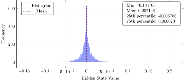
Figure 2: The histogram of FFN hidden state $\mathbf{h}$ for the $3$-th block and the $1,000$-th token.

As demonstrated in fig. 2, the distribution is sharply peaked at $0$ and constrained within a small range, indicating that most $h_{i}$ are concentrated near zero and confirming the sparsity. And it exhibits symmetry, suggesting a near-normal distribution centered around the mean. Based on what we discuss and observe above, the hidden state values work well as the basis for judgment of neuron activation, because of its high differentiation and independence across different neurons. Therefore, we propose a new metric, called absolute TopK (ATopK), to determine the activation status of a neuron with index $i$:

$$a_{i}=\left\{\begin{array}[]{rl}1,&\lvert h_{i}\rvert\in\text{TopK}(\{\lvert h_{j}\rvert\ |1\leq j\leq d_{h}\},K_{a}),\\ 0,&\text{otherwise},\end{array}\right.$$ (5)

where we choose neurons with $K_{a}$ highest absolute value among the hidden state values, and assign their labels in the activation marker $\mathbf{a}=\left[a_{1},a_{2},\cdots,a_{d_{h}}\right]$ with $1$.

To further evaluate the activation information, we make samples in the training set to record their activation markers. Given a batched input tensor $\mathbf{X}\in\mathbb{R}^{b\times s\times d}$, with $b$ the batch size and $s$ the sequence length, we obtain the batched hidden state $\mathbf{H}\in\mathbb{R}^{b\times s\times d_{h}}$ as follows:

$$\mathbf{H}=\text{Swish}(\mathbf{X}\mathbf{W}_{gate})\odot(\mathbf{X}\mathbf{W}_{up}).$$ (6)

Note that in practical implementation, we normalize $\mathbf{X}$, $\mathbf{W}_{gate}$ and $\mathbf{W}_{up}$ before the calculation to eliminate the influence of their magnitudes on the output. We then calculate the activation markers for the hidden state of all the tokens, which is reshaped as an activation feature matrix $\mathbf{A}\in\mathbb{R}^{q\times d_{h}},q=b\cdot s$. Denote the $i$-th column of $\mathbf{A}$ as the feature vector $\mathbf{c}_{i}\in\mathbb{R}^{q}$, i.e., $\mathbf{A}=[\mathbf{c}_{1}\;\mathbf{c}_{2}\;\cdots\;\mathbf{c}_{d_{h}}]$ which represents the $i$-th neuron’s activation status on the sampled $q$ tokens. By calculating the expected value of each $\mathbf{c}_{i}$, we can obtain the vector of activated rates $\bm{\mu}$ as:

$$\bm{\mu}=[\mu_{1},\mu_{2},\cdots,\mu_{d_{h}}],\mbox{ with }\mu_{i}=\frac{1}{q}\sum_{j=1}^{q}c_{j,i},$$ (7)

where $c_{j,i}$ indicates the $j$-th element of $\mathbf{c}_{i}$. We draw the histogram of $\bm{\mu}$ as in Fig. 3.

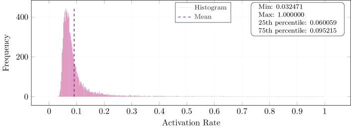
Figure 3: The histogram of activation rates $\bm{\mu}$ for the $3$-th block with $K_{a}=1,000$.

The histogram reveals a highly skewed distribution of activation rates, where the majority of neurons exhibit low activation rates (below 0.1), with a sharp peak near 0.07. However, the distribution also features a long tail, indicating the presence of a subset of neurons with significantly higher activation rates extending up to 1. These high-activation neurons are likely active across a wide range of input tokens, making them suitable for processing common knowledge rather than task-specific specialization. Therefore, we construct shared experts by grouping these high-activation neurons. Given the total number of shared experts as $N_{s}$ and the expert size $m$, we get the selection indices set $S_{N_{s}}$ by selecting $N_{s}\cdot m$ neurons with highest activation rates:

$$S_{N_{s}}=\{i\ :\ \mu_{i}\in\text{TopK}(\{\mu_{j}\mid 1\leq j\leq d_{h}\},N_{s}\cdot m)\}.$$ (8)

Since the independency across neurons, as we discussed, we build the experts using the same architecture as the original FFN and assign the expert parameters to the neurons of selected indices. Since all shared experts are always activated, we just construct them together for convenience:

$$\mathbf{W}_{up}^{s} =\mathbf{W}_{up}[:,S_{N_{s}}],$$ (9)

$$\mathbf{W}_{gate}^{s} =\mathbf{W}_{gate}[:,S_{N_{s}}],$$

$$\mathbf{W}_{down}^{s} =\mathbf{W}_{down}[S_{N_{s}},:],$$

where $\mathbf{W}_{up}^{s}\in\mathbb{R}^{d\times N_{s}\cdot m}$, $\mathbf{W}_{gate}^{s}\in\mathbb{R}^{d\times N_{s}\cdot m}$ and $\mathbf{W}_{down}^{s}\in\mathbb{R}^{N_{s}\cdot m\times d}$ are the weights of linear layers of the shared experts $E^{s}$. Given the input embedding $\mathbf{x}$, the output of $E^{s}$ is obtained via

$$E^{s}(\mathbf{x})\!=\!\mathbf{h}^{s}\mathbf{W}_{down}^{s},\mbox{ with }\mathbf{h}^{s}\!=\!\text{Swish}(\mathbf{x}\mathbf{W}_{gate}^{s})\!\odot\!(\mathbf{x}\mathbf{W}_{up}^{s}).$$

The majority of low activation rates also encourage us to construct routed experts, which are not always activated but are specialized for tokens encountered. To construct $N_{r}$ routed experts, we develop a customized balanced K-means clustering algorithm. We first identify $N_{r}$ centroids as the neurons (excluding those assigned to shared experts) with the highest activation rates, and group their feature vectors into a centroid set $C=\{\mathbf{c}_{i}:\mu_{i}\in\text{TopK}(\{\mu_{j}\mid 1\leq j\leq d_{h},j\notin S_{Ns}\},N_{r})\}=\{\hat{\mathbf{c}}_{1},\dots,\hat{\mathbf{c}}_{N_{r}}\}$, where, for convenience, we re-label the centroids with $\hat{\mathbf{c}}$.

By selecting these centroids, we ensure that the clusters are initialized around meaningful and prominent activation patterns, providing a strong starting point for clustering. Using the centroids selected, we will construct clusters with remaining neurons. We pay attention to their correlation to the centroids, i.e. we study the distances of their feature vectors to the centroids’. The feature vector $\mathbf{c}$ individually contains the activation status of a specific neuron, and we expect that neurons with similar functionalities will have similar patterns on the activation status, i.e. they are often activated and deactivated together during inference. Therefore, we compute the $L_{2}$ distance of each feature vector $\mathbf{c}$ to each centroid $\hat{\mathbf{c}}$. Define a distance matrix $\mathbf{D}\in\mathbb{R}^{N_{r}\cdot m\times N_{r}}$, whose element $d_{i,j}$ is the $L_{2}$ distance between the $i$-th feature vector $\mathbf{c}_{i}$ and the $j$-th centroid $\hat{\mathbf{c}}_{j}$:

$$d_{i,j}=\|\mathbf{c}_{i}-\hat{\mathbf{c}}_{j}\|_{2}=\sqrt{\sum_{k=1}^{q}(c_{k,i}-\hat{c}_{k,j})^{2}},$$ (10)

where, for convenience, we also include the original feature vectors of centroids inside the set to be grouped.

To group the neurons into routed experts, with the centroids designed above at $t=0$, the constrained balanced $K$-means clustering algorithm works as follows [31]. Given $N_{r}\cdot m$ vectors $\mathbf{c}$, the cluster membership value $m$ and cluster centroids $\hat{\mathbf{c}}_{1}^{t},\hat{\mathbf{c}}_{2}^{t},\dots,\hat{\mathbf{c}}_{N_{r}}^{t}$ at iteration $t$, compute $\hat{\mathbf{c}}_{1}^{t+1},\hat{\mathbf{c}}_{2}^{t+1},\dots,\hat{\mathbf{c}}_{N_{r}}^{t+1}$ at iteration $t+1$ with the following $2$ steps:

Cluster Assignment Let $T_{i,p}^{t}$ be a solution to the following linear program with $\hat{\mathbf{c}}_{p}^{t}$ fixed:

$$\min_{T} \sum_{i=1}^{N_{r}\cdot m}\sum_{p=1}^{N_{r}}T_{i,p}\cdot d_{i,p}$$ (11)

s.t. $$\sum_{i=1}^{N_{r}\cdot m}T_{i,p}=m,p=1,\dots N_{r}$$

$$\sum_{p=1}^{N_{r}}T_{i,p},i=1,\dots,N_{r}\cdot m$$

$$T_{i,p}\geq 0,i=1,\dots,N_{r}\cdot m,p=1,\dots N_{r}.$$

Cluster Update Update $\hat{\mathbf{c}}_{p}^{t+1}$ as follows:

$$\hat{\mathbf{c}}_{p}^{t+1}=\left\{\begin{array}[]{ll}\frac{\sum_{i=1}^{N_{r}\cdot m}T_{i,p}^{t}\cdot\mathbf{c}_{i}}{\sum_{i=1}^{N_{r}\cdot m}T_{i,p}^{t}},&\text{if}\sum_{i=1}^{N_{r}\cdot m}T_{i,p}^{t}>0,\\ \hat{\mathbf{c}}_{p}^{t},&\text{otherwise}.\end{array}\right.$$ (12)

The steps are terminated until $\hat{\mathbf{c}}_{p}^{t+1}=\hat{\mathbf{c}}_{p}^{t}$, $\forall p=1,\dots,N_{r}$.

We include the distance value $d_{i,j}$ into the cost function so that the balanced $K$-means clustering makes the intra-expert distances low and inter-expert distances high. However, the cluster assignment we defined above is an unbalanced assignment problem ($N_{r}\cdot m>m$) and cannot directly be solved by existing algorithms for balanced assignment. Therefore, we reduce it to a balanced assignment by extending the distance matrix $\mathbf{D}$ as follows:

$$\mathbf{D}^{ext} =\big{[}\underbrace{\mathbf{d}_{1},\dots,\mathbf{d}_{1}}_{m\text{ times}},\underbrace{\mathbf{d}_{2},\dots,\mathbf{d}_{2}}_{m\text{ times}},\dots,\underbrace{\mathbf{d}_{N_{r}},\dots,\mathbf{d}_{N_{r}}}_{m\text{ times}}\big{]},$$

where we repeat every column $\mathbf{d}$ of $\mathbf{D}$ $m$-times to obtain the extended matrix $\mathbf{D}^{ext}\in\mathbb{R}^{N_{r}\cdot m\times N_{r}\cdot m}$. Then the reduced balanced assignment problem is formulated as:

Balanced Assignment Let $T_{i,p^{\prime}}^{{}^{\prime},t}$ be a solution to the following linear program with $\hat{\mathbf{c}}_{p}^{t}$ fixed:

$$\min_{T^{\prime}} \sum_{i=1}^{N_{r}\cdot m}\sum_{p^{\prime}=1}^{N_{r}\cdot m}T^{\prime}_{i,p^{\prime}}\cdot d_{i,p^{\prime}}^{ext}$$ (13)

s.t. $$\sum_{i=1}^{N_{r}\cdot m}T^{\prime}_{i,p^{\prime}}=1,p^{\prime}=1,\dots N_{r}\cdot m$$

$$\sum_{p^{\prime}=1}^{N_{r}\cdot m}T^{\prime}_{i,p^{\prime}}=1,i=1,\dots,N_{r}\cdot m$$

$$T^{\prime}_{i,p^{\prime}}\geq 0,i=1,\dots,N_{r}\cdot m,p^{\prime}=1,\dots N_{r}\cdot m,$$

where $d_{i,p^{\prime}}^{ext}=d_{i,p}$ if $p\cdot m<p^{\prime}\leq(p+1)\cdot m$.

And the balanced cluster $\hat{\mathbf{c}}_{p}^{t+1}$ can be updated as follows:

$$\hat{\mathbf{c}}_{p}^{t+1}=\scriptstyle\left\{\begin{array}[]{ll}\frac{\sum\limits_{k=k_{0}}^{mp}\sum\limits_{i=1}^{N_{r}\cdot m}T_{i,k}^{{}^{\prime},t}\cdot\mathbf{c}_{i}}{\sum\limits_{k=k_{0}}^{mp}\sum\limits_{i=1}^{N_{r}\cdot m}T_{i,k}^{{}^{\prime},t}},&\text{if}\scriptstyle\sum\limits_{k=k_{0}}^{mp}\sum\limits_{i=1}^{N_{r}\cdot m}T_{i,k}^{{}^{\prime},t}>0,\\ \hat{\mathbf{c}}_{p}^{t},&\text{otherwise},\end{array}\right.$$ (14)

where $k_{0}=m(p-1)+1$. Drawing on the Jonker-Volgenant algorithm [32], this problem can be addressed as a reduced assignment problem in each step of the $K$-means algorithm, with a complexity of $O(n^{3})$.

The final solution $T^{\prime}$ gives us the optimized strategy to group the routed experts. We get the selection indices set $S_{N_{r},p}$, $p=1,\dots,N_{r}$, for each routed expert $E^{r}_{p}$:

$$S_{N_{r},p}=\{i\ :\exists\ T^{\prime}_{i,k}=1,\ \text{for}\ \forall k\in\{m(p-1)+1,\dots,m\}\}.$$

We then build the weights $\mathbf{W}_{up}^{r,p}\in\mathbb{R}^{d\times m}$, $\mathbf{W}_{gate}^{r,p}\in\mathbb{R}^{d\times m}$ and $\mathbf{W}_{down}^{r,p}\in\mathbb{R}^{m\times d}$ of each routed expert $E_{p}^{r}$ as in Equation 9. And the output of $E_{p}^{r}$ is given by:

$$E^{r}_{p}(\mathbf{x})\!=\!\mathbf{h}^{r}_{p}\mathbf{W}_{down}^{r,p},\mbox{ with }\mathbf{h}^{r}_{p}\!=\!\text{Swish}(\mathbf{x}\mathbf{W}_{gate}^{r,p})\odot(\mathbf{x}\mathbf{W}_{up}^{r,p}).$$

Suppose the MoE activates $N_{k}$ experts out of the $N_{r}$ routed experts. We expect the router to choose the routed experts with top $N_{k}$ scores. Therefore, we modify the MoE-version FFN as in (IV-A),

$$F_{MoE}(\mathbf{x}) =E^{s}(\mathbf{x})+\sum^{N_{r}}_{i=1}g_{i}E_{i}^{r}(\textbf{x}),$$

$$g_{i} =\left\{\begin{array}[]{rl}1,&s_{i}\in\text{TopK}(\{s_{i}|1\leq j\leq N_{r}\},N_{k}),\\ 0,&\text{otherwise},\end{array}\right.$$ (17)

s $$=\left[s_{1},s_{2},\cdots,s_{N_{r}}\right]=G(\textbf{x}),$$ (18)

where we make the expert score $g_{i}\in\{0,1\}$ to enable an un-scaled version of the expert output to avoid biases.

IV-B Training-free Router Construction

We now present the training-free router network $G$ for CMoE. Unlike previous works, which either built the router from scratch or intuitively used hidden features as initialization, we formulate the router construction as a minimization problem and then develop an algorithm with analysis to construct the router by approximating the optimal solution.

Given the same input embedding $\mathbf{x}$, the output of original output of the dense FFN, i.e. $F(\mathbf{x})$ in (1), is equivalent to the sum of the output of all the experts in $F_{MoE}$:

$$F(\mathbf{x}) =E^{s}(\mathbf{x})+\sum^{N_{r}}_{i=1}E_{i}^{r}(\textbf{x}).$$ (19)

The only difference between (19) and $F_{MoE}(\mathbf{x})$ in (IV-A) is the expert score $\mathbf{g}$, which is obtained from the TopK selection of the output of $G$. Therefore, to preserve important knowledge captured by the original dense FNN, $G$ can be constructed to enforce $F_{MoE}(\mathbf{x})$ to be close to $F(\mathbf{x})$ by solving the minimization problem (IV-B),

$$\arg\min_{G}|F_{MoE}(x;G)-F(x)|$$

$$=\! \!\arg\min_{G}|\sum^{N_{r}}_{i=1}(g_{i}-1)E_{i}^{r}(\textbf{x})|=\!\!\arg\min_{G}|\sum^{i\in S_{de}}E_{i}^{r}(\mathbf{x})|,$$

where $S_{de}\!=\!\{i:s_{i}\!\notin\!\text{TopK}(\{s_{i}|1\!\leq\!j\!\leq\!N_{r}\},N_{k})\}$ and $|S_{de}|\!=\!N_{r}\!-\!N_{k}$, and the problem becomes constructing the $G$ to minimize the absolute sum of the output of deactivated routed experts. Note that we have made a hypothesis in (4) that the output/sparsity of $F(x)$ is highly related to the norm/sparsity of $\mathbf{h}$, which is the same for the expert outputs. Based on (3) and (4), we reformulate (IV-B) as in (20):

$$\arg\min_{G}|\sum^{i\in S_{de}}E_{i}^{r}(\mathbf{x})|$$ (20)

$$\overset{\text{by}\ \eqref{eq:sum}}{=}\! \!\arg\min_{G}|\sum^{i\in S_{de}}\sum_{j\in S_{N_{r},i}}h_{j}\mathbf{w}_{down,j}|$$

$$\overset{\text{by}\ \eqref{eq:hypo}}{\approx}\! \!\arg\min_{G}|\sum^{i\in S_{de}}(\sum_{j\in S_{N_{r},i}}|h_{j}|)|$$

$$=\! \!\arg\min_{G}\mathbb{E}_{\mathbf{h}}\left[\|\mathbf{h}^{r}_{i}\|_{1}\mid i\in S_{de}\right].$$

The problem becomes constructing $G$ that can minimize the expected hidden states $\mathbf{h}$ of deactivated routed experts. Note that $G$ controls the de-/activation of routed experts by outputting the token-to-expert affinity $\mathbf{s}=[s_{1},\dots,s_{N_{r}}]$. Therefore, a solution for the above problem is to construct the $G$ such that matching the sorting indices of the set $\{s_{1},\dots,s_{N_{r}}\}$ and the set $\{\bar{\mathbf{h}}^{r}_{1},\dots,\bar{\mathbf{h}}^{r}_{N_{r}}\}$ ($\bar{\mathbf{h}}^{r}_{i}=\mathbb{E}_{\mathbf{h}}\left[||\mathbf{h}^{r}_{i}||_{1}\right]$), i.e. $\exists\ \text{permutation}\ \sigma\$ such that:

$$s_{\sigma(1)}\leq s_{\sigma(2)}\leq\dots\leq s_{\sigma(N_{r})}\mbox{ and}$$

$$\bar{\mathbf{h}}^{r}_{\sigma(1)}\leq\bar{\mathbf{h}}^{r}_{\sigma(2)}\leq\dots\leq\bar{\mathbf{h}}^{r}_{\sigma(N_{r})},$$ (21)

by which we can verify that the minimum of (20) is:

$$\min_{G}\ \mathbb{E}_{\mathbf{h}}\left[\|\mathbf{h}^{r}_{i}\|_{1}\mid i\in S_{de}\right]=\frac{1}{N_{r}-N_{k}}\!\!\sum_{i=1}^{N_{r}-N_{k}}\bar{\mathbf{h}}^{r}_{\sigma(i)},$$ (22)

which is obtained by setting $G(\mathbf{x})$ as:

$$S_{de} =\{\sigma(1),\dots,\sigma(N_{r}-N_{k})\}$$

$$=\{i:s_{i}\notin\text{TopK}(\{s_{i}|1\leq j\leq N_{r}\},N_{k})\}.$$ (23)

Finally, we pay attention to the hidden state $\mathbf{h}^{r}$ of any routed expert, which is the output by the neurons that we grouped in Section IV-A, where the cluster is centered to the centroid $\hat{\mathbf{c}}$. We denote the neuron in each cluster that has the lowest $L_{2}$ distance to the centroid as the representative neuron:

$$R_{j}=i,\mbox{ if }\|\mathbf{c}_{i}-\hat{\mathbf{c}}_{j}\|_{2}\leq\|\mathbf{c}_{k}-\hat{\mathbf{c}}_{j}\|_{2},\forall k\in S_{N_{r},j}.$$ (24)

Therefore, when we regard the hidden state value $h^{r}_{R_{j}}$ as feature of the representative neuron and assume that $h^{r}_{R_{j}}\approx\bar{\mathbf{h}}^{r}_{j}$, where $\bar{\mathbf{h}}^{r}_{j}$ refers to the expected hidden state value, we can construct the router by grouping the representative neurons of all the routed experts:

$$G(\mathbf{x}) =\text{Swish}(\mathbf{x}\mathbf{W}_{gate}^{R})\odot(\mathbf{x}\mathbf{W}_{up}^{R}),$$ (25)

where $\mathbf{W}_{gate}^{R}=\mathbf{W}_{gate}[:,S_{R}]$, $\mathbf{W}_{up}^{R}=\mathbf{W}_{up}[:,S_{R}]$, and $S_{R}=\{R_{1},\dots,R_{N_{r}}\}$. This leads to

$$G(\mathbf{x}) =\left[s_{1},s_{2},\cdots,s_{N_{r}}\right]=\left[h^{r}_{R_{1}},h^{r}_{R_{2}},\cdots,h^{r}_{R_{N_{r}}}\right]$$

$$\approx\left[\bar{\mathbf{h}}^{r}_{1},\mathbf{h}^{r}_{2},\cdots,\mathbf{h}^{r}_{N_{r}}\right],$$ (26)

which is hence an approximate solution for the original problem introduced in (IV-B).

IV-C Differentiable Routing and Load-balancing

Though we have constructed a well-designed router in Section IV-B, it is not differentiable since each expert score $g_{i}$ is a constant, as shown in (IV-A), hindering further alignment and performance recovery. Therefore, we introduce a learnable parameter $\mathbf{u}$ when computing the expert scores as follows,

$$g_{i}\! \!=\!\left\{\begin{array}[]{ll}\!\!1+s^{\prime}_{i}\cdot u_{i},&s^{\prime}_{i}\in\text{TopK}(\{s^{\prime}_{i}|1\leq j\leq N_{r}\},N_{k}),\\ \!\!0,&\text{otherwise},\end{array}\right.$$ (28)

$$\mathbf{s}^{\prime} =\text{Softmax}(\mathbf{s}),\ \textbf{u}=[u_{1},u_{2},\dots,u_{N_{r}}]$$ (29)

where the scale $\mathbf{u}$ is initialized as zero to avoid perturbation.

For MoE models, load-balancing is crucial to guarantee computational efficiency, especially expert parallelism in LLMs serving. As in DeepSeek-V3 [4], we use the auxiliary-loss-free load balancing by introducing a bias term $\mathbf{b}$ before the TopK selection:

$$g_{i}\! \!=\!\left\{\begin{array}[]{ll}\!\!1+s^{\prime}_{i}\cdot u_{i},&s^{\prime}_{i}+b_{i}\in\text{TopK}(\{s^{\prime}_{i}|1\leq j\leq N_{r}\},N_{k}),\\ \!\!0,&\text{otherwise},\end{array}\right.$$ (32)

$$\mathbf{b} =[b_{1},b_{2},\dots,b_{N_{r}}].$$ (33)

Here, $\mathbf{b}$ is initialized as zero and updated based on the expert load status during each step of training, as in DeepSeek-V3. The hyper-parameter update speed $\gamma$ is used to update the bias term $\mathbf{b}$ at the end of each step, i.e. decreasing/increasing the bias term by $\gamma$ if the corresponding expert is overloaded/underloaded.

V Experiments

TABLE I: Comparison of perplexity results. Randomly select samples from WikiText-2 training dataset for calibration and training.

Method Type LLaMA-2-7B LLaMA-3-8B Training-free Fine-tuning Training-free Fine-tuning WikiText-2 C4 WikiText-2 C4 WikiText-2 C4 WikiText-2 C4 Dense - 5.27 7.27 - - 6.14 9.44 - - LLaMA-MoE A2E8 nan nan 468.00 2660.68 nan nan 988.20 7521.83 LLaMA-MoE A4E16 nan nan 540.62 2690.68 nan nan 1094.24 7758.91 CMoE S1A1E8 60.86 135.61 12.76 32.12 162.74 324.71 21.16 64.03 CMoE S1A3E16 89.19 180.65 13.84 33.56 262.85 465.09 22.97 72.34 CMoE S2A2E16 62.30 136.12 12.73 32.37 143.38 284.19 21.01 65.57

CMoE is implemented based on Hugging Face Transformers [33] together with Pytorch [34]. The experiments are conducted on one NVIDIA H800 PCIe 80GB graphics card with CUDA Driver 12.6. We randomly select samples from WikiText-2 training dataset [35] as calibration and fine-tuning data. We use only 8 examples with 2,048 sequence length as calibration for calculating the hidden state $\mathbf{H}$ in (6). We set $K_{a}=10$ for the activation status record, which sounds counter-intuitive but works best in practice. For lightweight fine-tuning, we run $1$ epoch using the Adam optimizer [36] with $\beta_{1}$ = 0.9 and $\beta_{2}$ = 0.95. We also employ LoRA [37] with a rank of 8 and $lora\_alpha=32$. We fine-tune all the models including the baselines with $2,048$ samples. We set different initial learning rates for the score scale $\mathbf{u}$ and other parameters, i.e. $0.001$ and $5.95e^{-5}$, respectively. We set the bias update speed $\gamma$ to $0.001$.

V-A Main Results

We compare CMoE with the up-to-date baseline LLaMA-MoE [11], in which the neurons are randomly split, and continual pre-training is carried out with additional router networks. The experiments cover both training-free and lightweight fine-tuning versions. We design these experiments to demonstrate the remarkable post-training performance of CMoE. we demonstrate the results on two different datasets, i.e. WikiText-2 [35] and C4 [38]. The baseline models are chosen as LLaMA-2-7B and LLaMa-3-8B.

Language Modeling Performance. We evaluate the perplexity of the constructed Mixture-of-Experts (MoE) models in Table I. We use abbreviations to denote the composition of experts. For instance, ‘S2A2E16’ represents 2 shared experts, 2 activated routed experts, and a total of 16 experts and the total activation ratio is $(2+2)/16=25\%$. Our findings indicate that in the training-free scenario, the ppl of our baseline LLaMA-MoE on both LLaMA-2-7B and LLaMA-3-8B are NaN across different datasets. In contrast, the perplexity of the proposed CMoE can be effectively controlled. Moreover, after fine-tuning, we observe that the perplexity can be reduced to as low as 12.73 when the activation ratio is 25%, which corresponds to a sparsity of 75%. Additionally, the CMoE model outperforms all state-of-the-art (SOTA) structured pruning methods [9, 22, 23].

Downstream Tasks Performance. We also evaluate the performance of the constructed MoE models on various downstream tasks. We evaluate on the following benchmarks: 32-shot BoolQ [39], 0-shot PIQA [40], 0-shot SciQ [41], 5-shot Winogrande [42], 25-shot ARC-Challenge [43], and 10-shot HellaSwag [44]. The results are presented in table II, where we denote fine-tuning or not with ‘FT’. In all activation ratio configurations, we find that the proposed CMoE outperforms the LLaMA-MoE in accuracy across a diverse set of downstream tasks, on both training-free and fine-tuning scenarios.

To illustrate the performance of the models, we select the SciQ dataset for zero-shot testing and the BoolQ dataset for few-shot testing as representative examples. When the activation ratio is set at a fixed value of 25% (corresponding to a sparsity rate of 75%), after fine-tuning, the LLaMA-MoE model can only achieve an accuracy equivalent to 21.2% of that of the relevant dense model on the SciQ dataset and 45.31% on the BoolQ dataset. Given that the perplexity (ppl) of the LLaMA-MoE model is Not a Number (NaN) in the training-free scenario, we do not report its accuracy in this case. In contrast, even without fine-tuning (i.e., in the training-free scenario), the proposed CMoE model demonstrates superior performance, attaining an accuracy equivalent to 56.3% of that of the dense model on the SciQ dataset and 54% on the BoolQ dataset. After fine-tuning, the performance of the CMoE model is further enhanced, with the accuracy reaching 76.59% on the SciQ dataset and 74.3% on the BoolQ dataset (relative to dense model).

V-B Ablation Studies

We conduct ablation studies with LLaMA-2-7B and data randomly selected from WikiText-2 training datasets.

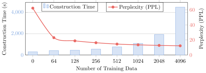
Figure 4: Trade-off between Model Performance and Construction Time with Increasing Training Data.

TABLE II: Comparison of downstream tasks. Randomly select samples from WikiText-2 training dataset as calibration and training data.

Model Method Type FT BoolQ(32) SciQ PIQA WinoGrande(5) ARC-C(25) HellaSwag(10) LLaMA-2-7B Dense - - 82.04 90.80 78.78 73.95 53.15 78.55 LLama-MoE A2E8 ✓ 37.83 20.00 49.73 50.12 25.79 26.18 LLama-MoE A4E16 ✓ 37.82 20.60 49.56 49.40 25.98 27.21 CMoE S1A1E8 ✗ 46.09 65.30 52.77 48.70 23.80 30.12 CMoE S1A3E16 ✗ 50.79 62.00 52.29 50.12 24.23 28.76 CMoE S2A2E16 ✗ 53.85 66.50 53.26 49.33 23.72 29.85 CMoE S1A1E8 ✓ 55.04 77.50 57.12 54.06 27.56 38.79 CMoE S1A3E16 ✓ 53.66 75.30 56.37 53.98 27.82 38.89 CMoE S2A2E16 ✓ 57.19 77.30 56.86 52.57 26.45 38.90 LLaMA-3-8B Dense - - 83.48 94.2 80.79 77.50 59.72 82.16 LLama-MoE A2E8 ✓ 37.82 20.30 49.02 50.74 25.68 25.76 LLama-MoE A4E16 ✓ 37.83 20.50 51.52 49.96 25.27 26.00 CMoE S1A1E8 ✗ 47.43 47.70 52.56 50.67 23.72 28.08 CMoE S1A3E16 ✗ 41.31 46.60 51.63 48.77 24.15 27.41 CMoE S2A2E16 ✗ 45.08 53.10 50.87 53.19 24.23 28.44 CMoE S1A1E8 ✓ 56.88 72.00 57.34 51.93 25.77 36.68 CMoE S1A3E16 ✓ 60.55 71.40 57.07 53.51 26.54 36.28 CMoE S2A2E16 ✓ 62.14 72.20 59.08 51.14 27.73 36.68

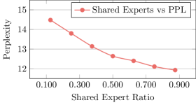
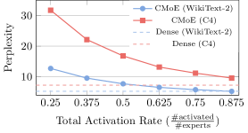
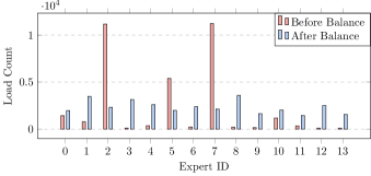
Figure 5: Ablation studies:(a) Impact of shared expert ratio on model performance; (b) Activation Rate vs. Model Performance; (c) Effect of Load Balancing.

Impact of Training Data Size. To quantify the relationship between training data volume, model performance, and computational efficiency, we systematically vary the number of training samples from 0 (initial state) to 4,096 while measuring perplexity (PPL) and construction time. Fig. 4 illustrates the results on the setting of “S2A2E16”, revealing critical trends in performance-cost trade-offs.

Increasing training data from 0 to 4,096 samples reduces perplexity by 80.4% (62.30 $\to$ 12.21) but non-linearly increases construction time from 298s to 4,502s. While performance improves sharply initially (64 samples cut PPL by 63%), gains diminish beyond 1,024 samples (13.47 PPL), with marginal improvements (12.21 PPL at 4,096 samples) requiring disproportionately higher runtime (+133% from 2,048 to 4,096 samples). The results demonstrate that CMoE only needs a modest of data to achieve low perplexity, while further performance increase is hard and possibly demands more diverse data.

Shared Experts Ratio. We carry out an extensive analysis of the influence of the shared expert ratio on perplexity. In our experimental setup, we have a total of 32 experts, among which 8 are activated. We systematically adjust the proportion of shared experts within these 8 activated experts. As depicted in Table Fig. 5, the results clearly demonstrate a distinct trend: as the ratio of shared experts rises from 0.125 to 0.875, the perplexity continuously decreases. There is a remarkable improvement in the perplexity value, dropping from 14.48 to 11.93. This finding indicates that shared experts generally contribute positively to the performance of the model. However, it is also evident that the marginal returns tend to diminish when the ratio of shared experts reaches a relatively high level.

Activation Rate. We conduct an external analysis to investigate how the total activation rate (comprising both shared and activated routed experts) impacts model performance across different domains, in comparison with dense baselines. We perform evaluations on the CMoE model featuring a total of 16 experts. Specifically, we vary the ratio of shared experts and activated routed experts at a fixed proportion of 1:1 on the WikiText-2 and C4 datasets. As illustrated in Table Fig. 5, a monotonic decrease in PPL can be found as the activation rate increases, gradually approaching the performance level of the dense model. For both datasets, an activation rate of 75% enables the model to achieve nearly comparable performance to the dense model. On the WikiText-2 dataset, the PPL values are 5.79 for the model under consideration and 5.27 for the dense model; on the C4 dataset, the corresponding values are 11.19 and 7.27. These results demonstrate that CMoE architectures can attain a performance quality comparable to that of dense models, even when characterized by relatively high sparsity.

Load Balancing. CMoE can inherently achieve effective load-balancing among routed experts, with the exception of some special blocks. For example, the last block of LLaMA-2-7B exhibits extremely unbalanced expert counts. However, this issue can be effectively resolved by the load-balancing mechanism we introduced in Section IV-C. As presented in Fig. 5, prior to the implementation of the load-balancing strategy, substantial disparities in the workloads assigned to different experts are clearly observable. Specifically, Expert 3 and Expert 8 are burdened with disproportionately high loads, handling 11,163 and 11,225 instances respectively. In stark contrast, other experts process a significantly lower number of instances. For example, Expert 12 and Expert 13 handle only 100 and 102 instances respectively. Upon the application of our proposed load - balancing mechanism, a more equitable and uniform distribution of the computational workload across all experts is successfully achieved. After the adjustment, the number of instances processed by each expert falls within the range of 1,443 to 3,584.

VI Conclusion

We present CMoE, a framework that efficiently carves sparse Mixture-of-Experts (MoE) architectures from dense LLMs through parameter reorganization and lightweight adaptation. By leveraging activation sparsity patterns in FFN layers, CMoE groups neurons into shared and routed experts via a novel balanced linear assignment formulation. The router is analytically initialized from activation statistics and refined via differentiable scaling and load balancing. Experiments show that CMoE can construct effective Mixture-of-Experts (MoE) models, achieving comparable perplexity to dense models and outperforming baseline models. For instance, on the SciQ dataset, CMoE can reach 56.3% even without fine-tuning and it can further improve the accuracy to 76.59% after fine-tuning, a huge outperforming compared with 21.2% (the accuracy of the baseline LLaMA-MoE). Extensive experiments have demonstrated that CMoE offers a practical approach for deploying large language models (LLMs) in resource-constrained environments.

References

- [1] S. Zhang, S. Roller, N. Goyal, M. Artetxe, M. Chen, S. Chen, C. Dewan, M. Diab, X. Li, X. V. Lin et al., “Opt: Open pre-trained transformer language models,” arXiv preprint arXiv:2205.01068, 2022.
- [2] H. Touvron, L. Martin, K. Stone, P. Albert, A. Almahairi, Y. Babaei, N. Bashlykov, S. Batra, P. Bhargava, S. Bhosale et al., “Llama 2: Open foundation and fine-tuned chat models,” arXiv preprint arXiv:2307.09288, 2023.
- [3] H. Liu, C. Li, Q. Wu, and Y. J. Lee, “Visual instruction tuning,” Advances in neural information processing systems, vol. 36, 2024.
- [4] A. Liu, B. Feng, B. Xue, B. Wang, B. Wu, C. Lu, C. Zhao, C. Deng, C. Zhang, C. Ruan et al., “Deepseek-v3 technical report,” arXiv preprint arXiv:2412.19437, 2024.
- [5] D. Lepikhin, H. Lee, Y. Xu, D. Chen, O. Firat, Y. Huang, M. Krikun, N. Shazeer, and Z. Chen, “Gshard: Scaling giant models with conditional computation and automatic sharding,” arXiv preprint arXiv:2006.16668, 2020.
- [6] N. Du, Y. Huang, A. M. Dai, S. Tong, D. Lepikhin, Y. Xu, M. Krikun, Y. Zhou, A. W. Yu, O. Firat et al., “Glam: Efficient scaling of language models with mixture-of-experts,” in International Conference on Machine Learning. PMLR, 2022, pp. 5547–5569.
- [7] W. Fedus, B. Zoph, and N. Shazeer, “Switch transformers: Scaling to trillion parameter models with simple and efficient sparsity,” Journal of Machine Learning Research, vol. 23, no. 120, pp. 1–39, 2022.
- [8] D. Dai, C. Deng, C. Zhao, R. Xu, H. Gao, D. Chen, J. Li, W. Zeng, X. Yu, Y. Wu et al., “Deepseekmoe: Towards ultimate expert specialization in mixture-of-experts language models,” arXiv preprint arXiv:2401.06066, 2024.
- [9] Z. Liu, J. Wang, T. Dao, T. Zhou, B. Yuan, Z. Song, A. Shrivastava, C. Zhang, Y. Tian, C. Re et al., “Deja vu: Contextual sparsity for efficient llms at inference time,” in International Conference on Machine Learning. PMLR, 2023, pp. 22 137–22 176.
- [10] Z. Zhang, Y. Lin, Z. Liu, P. Li, M. Sun, and J. Zhou, “Moefication: Transformer feed-forward layers are mixtures of experts,” arXiv preprint arXiv:2110.01786, 2021.
- [11] T. Zhu, X. Qu, D. Dong, J. Ruan, J. Tong, C. He, and Y. Cheng, “Llama-moe: Building mixture-of-experts from llama with continual pre-training,” in Proceedings of the 2024 Conference on Empirical Methods in Natural Language Processing, 2024, pp. 15 913–15 923.
- [12] X. Qu, D. Dong, X. Hu, T. Zhu, W. Sun, and Y. Cheng, “Llama-moe v2: Exploring sparsity of llama from perspective of mixture-of-experts with post-training,” arXiv preprint arXiv:2411.15708, 2024.
- [13] H. Zheng, X. Bai, X. Liu, Z. M. Mao, B. Chen, F. Lai, and A. Prakash, “Learn to be efficient: Build structured sparsity in large language models,” arXiv preprint arXiv:2402.06126, 2024.
- [14] S. Zuo, Q. Zhang, C. Liang, P. He, T. Zhao, and W. Chen, “Moebert: from bert to mixture-of-experts via importance-guided adaptation,” arXiv preprint arXiv:2204.07675, 2022.
- [15] A. Komatsuzaki, J. Puigcerver, J. Lee-Thorp, C. R. Ruiz, B. Mustafa, J. Ainslie, Y. Tay, M. Dehghani, and N. Houlsby, “Sparse upcycling: Training mixture-of-experts from dense checkpoints,” arXiv preprint arXiv:2212.05055, 2022.
- [16] H. Wu, H. Zheng, Z. He, and B. Yu, “Parameter-efficient sparsity crafting from dense to mixture-of-experts for instruction tuning on general tasks,” arXiv preprint arXiv:2401.02731, 2024.
- [17] J. Lin, J. Tang, H. Tang, S. Yang, W.-M. Chen, W.-C. Wang, G. Xiao, X. Dang, C. Gan, and S. Han, “Awq: Activation-aware weight quantization for on-device llm compression and acceleration,” Proceedings of Machine Learning and Systems, vol. 6, pp. 87–100, 2024.
- [18] Z. Pei, X. Yao, W. Zhao, and B. Yu, “Quantization via distillation and contrastive learning,” IEEE Transactions on Neural Networks and Learning Systems, 2023.
- [19] L. Zou, W. Zhao, S. Yin, C. Bai, Q. Sun, and B. Yu, “Bie: Bi-exponent block floating-point for large language models quantization,” in Forty-first International Conference on Machine Learning, 2024.
- [20] Y. Lin, H. Tang, S. Yang, Z. Zhang, G. Xiao, C. Gan, and S. Han, “Qserve: W4a8kv4 quantization and system co-design for efficient llm serving,” arXiv preprint arXiv:2405.04532, 2024.
- [21] X. Men, M. Xu, Q. Zhang, B. Wang, H. Lin, Y. Lu, X. Han, and W. Chen, “Shortgpt: Layers in large language models are more redundant than you expect,” arXiv preprint arXiv:2403.03853, 2024.
- [22] S. Ashkboos, M. L. Croci, M. G. d. Nascimento, T. Hoefler, and J. Hensman, “Slicegpt: Compress large language models by deleting rows and columns,” arXiv preprint arXiv:2401.15024, 2024.
- [23] Z. Pei, H.-L. Zhen, X. Yu, S. J. Pan, M. Yuan, and B. Yu, “Fusegpt: Learnable layers fusion of generative pre-trained transformers,” arXiv preprint arXiv:2411.14507, 2024.
- [24] H. Zheng, X. Bai, X. Liu, Z. M. Mao, B. Chen, F. Lai, and A. Prakash, “Learn to be efficient: Build structured sparsity in large language models,” arXiv preprint arXiv:2402.06126, 2024.
- [25] A. Dubey, A. Jauhri, A. Pandey, A. Kadian, A. Al-Dahle, A. Letman, A. Mathur, A. Schelten, A. Yang, A. Fan et al., “The llama 3 herd of models,” arXiv preprint arXiv:2407.21783, 2024.
- [26] N. Shazeer, “Glu variants improve transformer,” arXiv preprint arXiv:2002.05202, 2020.
- [27] V. Nair and G. E. Hinton, “Rectified linear units improve restricted boltzmann machines,” in Proceedings of the 27th international conference on machine learning (ICML-10), 2010, pp. 807–814.
- [28] Z. Zhang, Y. Lin, Z. Liu, P. Li, M. Sun, and J. Zhou, “Moefication: Transformer feed-forward layers are mixtures of experts,” arXiv preprint arXiv:2110.01786, 2021.
- [29] J. Song, K. Oh, T. Kim, H. Kim, Y. Kim, and J.-J. Kim, “Sleb: Streamlining llms through redundancy verification and elimination of transformer blocks,” arXiv preprint arXiv:2402.09025, 2024.
- [30] X. Chen, Y. Hu, and J. Zhang, “Compressing large language models by streamlining the unimportant layer,” arXiv preprint arXiv:2403.19135, 2024.
- [31] M. I. Malinen and P. Fränti, “Balanced k-means for clustering,” in Structural, Syntactic, and Statistical Pattern Recognition: Joint IAPR International Workshop, S+ SSPR 2014, Joensuu, Finland, August 20-22, 2014. Proceedings. Springer, 2014, pp. 32–41.
- [32] R. Jonker and T. Volgenant, “A shortest augmenting path algorithm for dense and sparse linear assignment problems,” in DGOR/NSOR: Papers of the 16th Annual Meeting of DGOR in Cooperation with NSOR/Vorträge der 16. Jahrestagung der DGOR zusammen mit der NSOR. Springer, 1988, pp. 622–622.
- [33] T. Wolf, “Huggingface’s transformers: State-of-the-art natural language processing,” arXiv preprint arXiv:1910.03771, 2019.
- [34] A. Paszke, S. Gross, F. Massa, A. Lerer, J. Bradbury, G. Chanan, T. Killeen, Z. Lin, N. Gimelshein, L. Antiga et al., “Pytorch: An imperative style, high-performance deep learning library,” Advances in neural information processing systems, vol. 32, 2019.
- [35] S. Merity, C. Xiong, J. Bradbury, and R. Socher, “Pointer sentinel mixture models,” arXiv preprint arXiv:1609.07843, 2016.
- [36] D. P. Kingma, “Adam: A method for stochastic optimization,” arXiv preprint arXiv:1412.6980, 2014.
- [37] E. J. Hu, Y. Shen, P. Wallis, Z. Allen-Zhu, Y. Li, S. Wang, L. Wang, and W. Chen, “Lora: Low-rank adaptation of large language models,” arXiv preprint arXiv:2106.09685, 2021.
- [38] C. Raffel, N. Shazeer, A. Roberts, K. Lee, S. Narang, M. Matena, Y. Zhou, W. Li, and P. J. Liu, “Exploring the limits of transfer learning with a unified text-to-text transformer,” Journal of machine learning research, vol. 21, no. 140, pp. 1–67, 2020.
- [39] C. Clark, K. Lee, M.-W. Chang, T. Kwiatkowski, M. Collins, and K. Toutanova, “Boolq: Exploring the surprising difficulty of natural yes/no questions,” arXiv preprint arXiv:1905.10044, 2019.
- [40] Y. Bisk, R. Zellers, J. Gao, Y. Choi et al., “Piqa: Reasoning about physical commonsense in natural language,” in Proceedings of the AAAI conference on artificial intelligence, vol. 34, no. 05, 2020, pp. 7432–7439.
- [41] J. Welbl, N. F. Liu, and M. Gardner, “Crowdsourcing multiple choice science questions,” arXiv preprint arXiv:1707.06209, 2017.
- [42] K. Sakaguchi, R. L. Bras, C. Bhagavatula, and Y. Choi, “Winogrande: An adversarial winograd schema challenge at scale,” Communications of the ACM, vol. 64, no. 9, pp. 99–106, 2021.
- [43] P. Clark, I. Cowhey, O. Etzioni, T. Khot, A. Sabharwal, C. Schoenick, and O. Tafjord, “Think you have solved question answering? try arc, the ai2 reasoning challenge,” arXiv preprint arXiv:1803.05457, 2018.
- [44] R. Zellers, A. Holtzman, Y. Bisk, A. Farhadi, and Y. Choi, “Hellaswag: Can a machine really finish your sentence?” arXiv preprint arXiv:1905.07830, 2019.