Phonon spectra, quantum geometry, and the Goldstone theorem

Abstract

Phonons are essential (quasi)particles of all crystals and play a key role in fundamental properties such as thermal transport and superconductivity. In particular, acoustic phonons can be viewed as the Goldstone modes arising from the spontaneous breaking of translational symmetry. In this article, we present a comprehensive—in the absence of Holstein phonons—theory of the quantum geometric contributions to the phonon spectra of crystals. Using graphene as a case study, we separate the dynamical matrix into several terms that depend differently on the electron energy and wavefunction, and demonstrate that the quantum geometric effects are crucial in shaping the phonon spectra of the material. Neglecting them leads to a gap in the acoustic phonon branches, which clearly violates the Goldstone theorem.

Introduction.—Every crystal supports elastic waves, which are traveling quanta of vibrational energy [1, 2] that Frenkel dubbed “phonons” in 1932. Phonons are quasiparticles that appear in a wide variety of condensed matter phenomena. Most notably, they serve as the bosonic glue that binds electrons into Cooper pairs in many conventional BCS superconductors [3]. They also play crucial roles in thermal and electrical transport, acting as an intrinsic and unavoidable source of scattering for electrons moving through a crystal. Additionally, phonons are important in atomically thin two-dimensional (2D) materials [4]: the authors of Ref. [5] demonstrated that graphene samples encapsulated in hexagonal Boron Nitride can display very large mobilities also at room temperature, which are solely limited by scattering of electrons against graphene’s acoustic phonons [6, 7, 8, 9, 10]. These are gapless modes near the center of the first Brillouin zone (FBZ)—see black lines labelled by “LA” and “TA” in Fig. 1—and play an important role in limiting plasmon lifetimes [11, 12, 13, 14] in the same devices. From a theoretical point of view, acoustic phonons can be thought of as the Goldstones associated with the spontaneous breaking of continuous translation symmetry [15, 18, 17, 16].

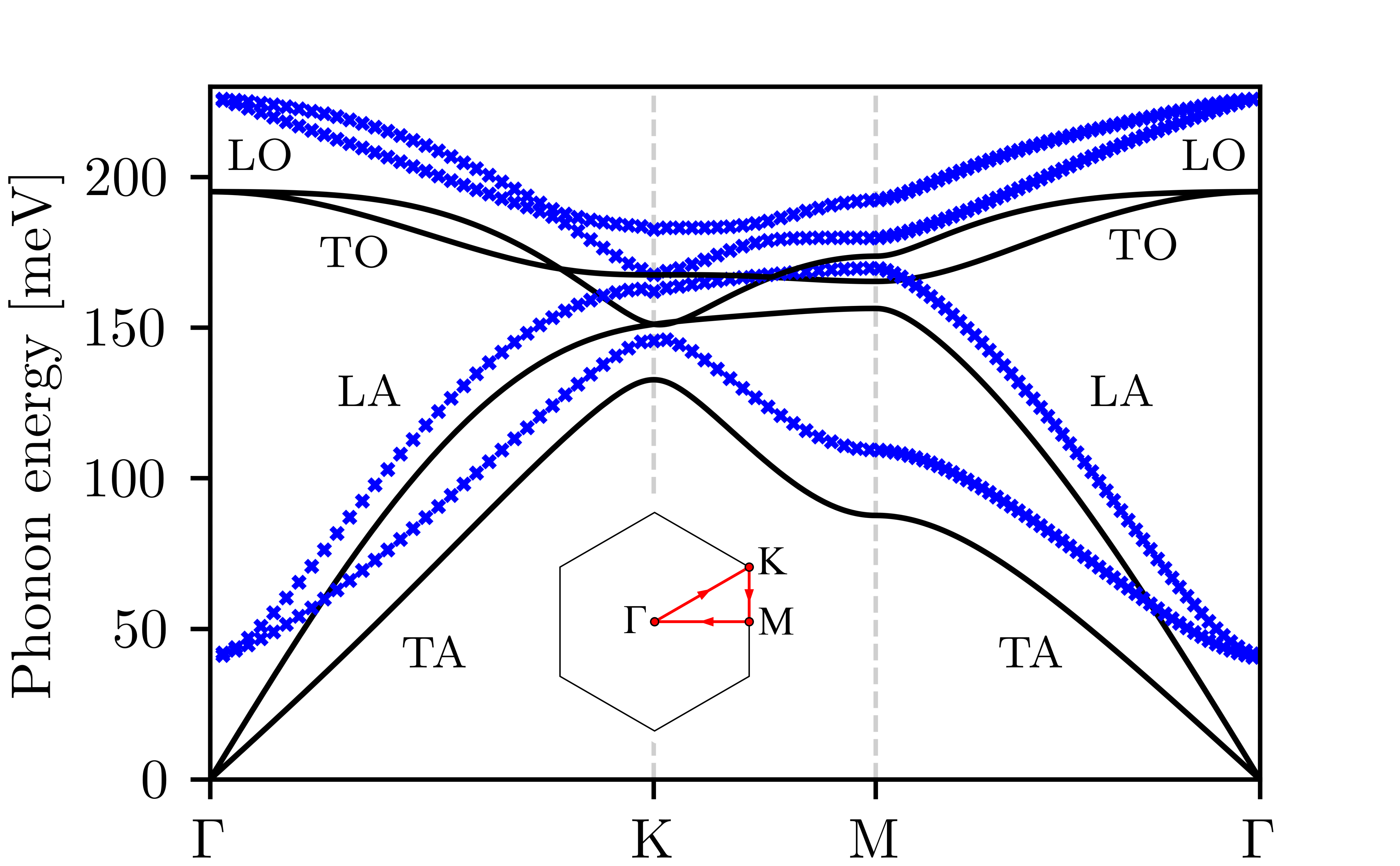
Figure 1: (Color online) Dispersion of the four in-plane phonon branches (LA, TA, LO, and TO) in graphene. Results in this figure are plotted along the $\Gamma$KM$\Gamma$ high-symmetry path in the first Brillouin zone illustrated in the inset. Black lines: Phonon dispersion $\omega_{\ell}(\bm{q})$ calculated analytically within a next-nearest neighbor Born-von Karman framework [66]. The relevant parameters needed to produce these plots have been determined by fitting ab initio density functional theory results. Blue crosses: Phonon dispersion $\tilde{\omega}_{\ell}(\bm{q})$ as calculated after removing from the full dynamical matrix ${\cal D}({\bm{q}})$ the quantum geometric contribution ${\cal D}_{\rm g}({\bm{q}})$—see Eqs. (27)-(28). Note that the dispersion represented by blue crosses violates the Goldstone theorem [15, 18, 17, 16].

The physical properties listed above depend critically on the electron-phonon interaction (EPI) [19, 20]. The coexistence of electrons and phonons in a single host crystal has recently prompted various authors to search for topological contributions to phonons that originate microscopically from the EPI (see, for example, Refs. [21] and [22]). After two decades of intense research on applying topology to material science properties [23, 24, 26, 25], a more general mathematical framework—now universally known as “quantum geometry”—is attracting significant attention in the community [27, 28]. In 1980, Provost and Vallee [29] understood that the usual Hermitian product on the projective Hilbert space induces a meaningful metric tensor on any manifold of quantum states. This intuition led them to introduce the quantum geometric tensor (QGT):

$$\mathcal{Q}_{ij}(\bm{k})=g_{ij}({\bm{k}})-\frac{i}{2}{\cal F}_{ij}({\bm{k}})~.$$ (1)

Here, $g_{ij}({\bm{k}})$ is a real, symmetric, and gauge-invariant tensor usually dubbed quantum metric (or Fubini-Study metric [30, 31]) and defined by

$$g_{ij}({\bm{k}})=\operatorname{Re}\bigl{[}\left\langle\partial_{k_{i}}\psi_{\bm{k}}\middle|\partial_{k_{j}}\psi_{\bm{k}}\right\rangle\bigr{]}-\left\langle\partial_{k_{i}}\psi_{\bm{k}}\middle|\psi_{\bm{k}}\right\rangle\left\langle\psi_{\bm{k}}\middle|\partial_{k_{j}}\psi_{\bm{k}}\right\rangle~.$$ (2)

Here, $\{|\psi_{\bm{k}}\rangle\}$ is a family of normalized vectors of some Hilbert space which smoothly depend on an $n$-dimensional parameter ${\bm{k}}\in{\mathbb{R}}^{n}$ (this is usually the Bloch quasi-momentum in solid-state physics). The quantum metric tensor $g_{ij}({\bm{k}})$ is a measure of the distance in amplitude between infinitesimally close wavefunctions in ${\bm{k}}$-space.

The second term in Eq. (1) is instead the more familiar Berry curvature [32, 24, 26]:

$${\cal F}_{ij}({\bm{k}}) =\left\langle\partial_{k_{i}}\psi_{\bm{k}}\middle|\partial_{k_{j}}\psi_{\bm{k}}\right\rangle-\left\langle\partial_{k_{j}}\psi_{\bm{k}}\middle|\partial_{k_{i}}\psi_{\bm{k}}\right\rangle$$

$$=2i\operatorname{Im}\left\langle\partial_{k_{i}}\psi_{\bm{k}}\middle|\partial_{k_{j}}\psi_{\bm{k}}\right\rangle~,$$ (3)

which, of course, is also gauge invariant. A more modern and compact definition of the QGT is provided below in Eq. (21) and in App. I of the Supplemental Material [33].

The QGT plays a fundamental role in a vast number of physical phenomena. Its importance in the theory of the insulating state, for example, has been known for more than two decades [34, 35, 36], and has been recently revisited [40, 41, 39, 37, 38]. Interest in the QGT has been recently revitalized in the context of strongly correlated electron systems with flat bands such as flat-band superconductors [42, 43, 45, 46, 44, 47, 48]. Quantum transport anomalies in systems with flat bands [49] as well as nonlinear optical response functions [50] have also been linked to the quantum geometry of states. Direct measurements of the QGT have been reported in optical lattices [51], qubits [52, 53], microcavities [54], and, more recently, in moiré materials [55]; however, further experimental replication is necessary.

A recent theoretical work [56] has incorporated the quantum geometry of the electron bands into the theory of EPIs, demonstrating the crucial contributions of the Fubini–Study metric [30] or its orbital selective version [56] to the dimensionless electron-phonon coupling constant. Concrete estimates have been provided for two materials, i.e. graphene and ${\rm MgB}_{2}$, where the geometric contributions account for approximately $50\%$ and $90\%$ of the total electron-phonon coupling constant, respectively. In this work, we study the role of the QGT on the phonon dispersion directly, using the same Gaussian approximation introduced in Ref. [56]. We do not consider Holstein-type EPI [57, 58, 59], for which the approximation used fails. Ions in the lattice experience both their mutual repulsion and the attractive force of the electron cloud. The latter is represented, within the Born-Oppenheimer approximation [1], by the variation of the electronic ground-state energy induced by the displacement of an ion from its equilibrium position. We show that this electronic term in the ionic equation of motion contains a contribution which is entirely due to the electronic QGT, thus affecting the phonon dispersion of the crystal. We calculate the geometric contribution to phonon dispersion analytically as a function of momentum, thereby providing the first ${\bm{k}}$-resolved quantifier of the impact of the electron geometry on the ionic motion. We then choose graphene as a case study. The choice of this material is well motivated: it exhibits a non-zero QGT due to its two-site unit cell, the electron dispersion relation in graphene is very well-described by a simple tight-binding model, and the EPI has already been benchmarked in [56] to be well-described by the approximation used here. We find that removing the non-trivial quantum geometric contribution from the calculation of phonons deeply affects the vibrational modes of this material, as clearly seen in Fig. 1. Removing the quantum geometric contribution spoils the massless nature of acoustic phonons, thus tampering with the above-mentioned Goldstone theorem.

Harmonic theory of phonons and Goldstone sum rules.—Consider a generic multipartite lattice in $D$ dimensions, with $N_{\bm{\tau}}$ atoms in the unit cell. In the following, we will denote with $\bm{R}_{p\nu}\equiv\bm{R}_{p}+\bm{\tau}_{\nu\vphantom{{}^{\prime}}}+\bm{u}_{p\nu\vphantom{{}^{\prime}}}\in{\mathbb{R}}^{D}$ the position of the ions in the lattice, where $\bm{R}_{p}$ is a Bravais lattice vector labelled by an integer $p=1,\dots,N$ in a finite $N$-unit-cell Born-von Karman (BvK) supercell [19], $\bm{\tau}_{\nu\vphantom{{}^{\prime}}}$ is a basis vector in the $\bm{R}_{p}=\bm{0}$ unit cell labelled by a sublattice number $\nu=1,\dots,N_{\bm{\tau}}$, and $\bm{u}_{p\nu}$ is the displacement of an ion from its equilibrium position $\bm{R}^{0}_{p\nu}\equiv\bm{R}_{p}+\bm{\tau}_{\nu}$.

Choosing a basis $\{\varphi_{\nu\alpha}(\bm{r})\}$ of sufficiently localized wavefunctions, the second-quantized one-electron Hamiltonian in the modified [56] tight-binding model can be expressed as

$$\hat{{\cal H}}_{{\rm e}}(\{\bm{u}_{p\nu}\})=\sum_{p\nu\alpha\vphantom{{}^{\prime}}}\sum_{p^{\prime}\nu^{\prime}\alpha^{\prime}}t_{\nu\nu^{\prime}}^{\alpha\alpha^{\prime}}\left(\bm{R}_{p\nu}-\bm{R}_{p^{\prime}\nu^{\prime}}\right)\hat{c}^{\dagger}_{p\nu\alpha\vphantom{{}^{\prime}}}\hat{c}^{\vphantom{\dagger}}_{p^{\prime}\nu^{\prime}\alpha^{\prime}}~,$$ (4)

where $\hat{c}^{\dagger}_{p\nu\alpha\vphantom{{}^{\prime}}}$ creates an electron in a generic orbital state identified by an additional set of quantum numbers $\alpha$ (including e.g. spin or internal atomic degrees of freedom) on the lattice site $\bm{R}^{0}_{p\nu}$, and $t^{\alpha\alpha^{\prime}}_{\nu\nu^{\prime}}(\bm{r})=[t(\bm{r})]_{\nu\nu^{\prime}}^{\alpha\alpha^{\prime}}$ denotes the matrix elements of the hopping matrix $t({\bm{r}})$, which carries both sublattice and orbital indices. Each matrix element is a smooth hopping function satisfying $[t(-\bm{r})]_{\nu\nu^{\prime}}^{\alpha\alpha^{\prime}}=[t^{*}(\bm{r})]_{\nu\nu^{\prime}}^{\alpha\alpha^{\prime}}$ in order to guarantee the Hermiticity of $\hat{\cal H}_{\rm e}(\{\bm{u}_{p\nu}\})$.

The Hamiltonian (4), the many-electron ground state $|\phi^{(0)}_{\{\bm{u}_{p\nu}\}}\rangle$, and the electronic contribution $\mathcal{E}_{0}(\{\bm{u}_{p\nu}\})$ to the ground-state energy,

$$\mathcal{E}_{0}(\{\bm{u}_{p\nu}\})\equiv\left\langle\phi^{(0)}_{\{\bm{u}_{p\nu}\}}\middle|\hat{\cal H}_{\rm e}(\{\bm{u}_{p\nu}\})\middle|\phi^{(0)}_{\{\bm{u}_{p\nu}\}}\right\rangle~,$$ (5)

depend parametrically on the set of displacements $\left\{\bm{u}_{p\nu}\right\}$ of the ions from their equilibrium positions. Both the ground state and the ground-state energy, as well as the Hamiltonian’s excited eigenstates introduced below, are evaluated within the one-electron approximation. Generalizations to include electron-electron interactions are of course possible in the spirit of density functional perturbation theory [19] but are beyond the scope of the present work.

The standard tight-binding formalism is recovered by employing the Born-Oppenheimer approximation (BOA) [1], where the ions are assumed to be frozen in a fixed configuration while solving for the electronic degrees of freedom. In the BOA, the classical ionic Hamiltonian can be expanded up to second order in the ionic displacements (harmonic approximation) as follows:

$$\hat{\cal H}_{\text{ion}}=\sum_{p\nu}\frac{\bm{P}^{2}_{p\nu}}{2M_{\nu}}+\frac{1}{2}\sum_{pp^{\prime}}\sum_{\nu\nu^{\prime}}\sum_{ij}\bigl{[}{\cal C}\bigr{]}_{p\nu i}^{p^{\prime}\nu^{\prime}j}u_{p\nu i}u_{p^{\prime}\nu^{\prime}j}~,$$ (6)

where $i,j$ are Cartesian indices and we have defined the inter-atomic force constants as

$$\begin{split}\bigl{[}{\cal C}\bigr{]}_{p\nu i}^{p^{\prime}\nu^{\prime}j}&\equiv\bigl{[}{\cal C}^{(\text{ion})}\bigr{]}_{p\nu i}^{p^{\prime}\nu^{\prime}j}+\bigl{[}{\cal C}^{(\text{el})}\bigr{]}_{p\nu i}^{p^{\prime}\nu^{\prime}j}\\ &=\left.\frac{\partial^{2}\mathcal{V}}{\partial u_{p\nu i}\,\partial u_{p^{\prime}\nu^{\prime}j}}\right|_{0}+\left.\frac{\partial^{2}\mathcal{E}_{0}}{\partial u_{p\nu i}\,\partial u_{p^{\prime}\nu^{\prime}j}}\right|_{0}~.\end{split}$$ (7)

This expression of the inter-atomic force constants highlights the natural separation into a term due to the ion-ion repulsive interactions, i.e. the first term in Eq. (7), and one which depends on the electronic degrees of freedom only, i.e. the second term in Eq. (7). Here and in what follows, the symbol $\left.A\right|_{0}$ denotes that the quantity $A$ is evaluated at the mechanical equilibrium configuration, i.e. for $\{{\bm{u}}_{p\nu}={\bm{0}}\}$. Consistently with the above mentioned one-electron approximation, the equilibrium-configuration ground state $|\phi^{(0)}_{\{{\bm{0}}\}}\rangle\equiv|\phi^{(0)}_{\{{\bm{u}_{p\nu}}={\bm{0}}\}}\rangle$ is taken to be the non-interacting Fermi sea [60].

We are now ready to introduce the dynamical matrix, whose diagonalization results in the phonon dispersion. Indeed, the dispersion $\omega_{\ell}(\bm{q})$ of the $\ell$-th phononic branch, where $\ell=1,\dots,D\times N_{\bm{\tau}}$ and $\bm{q}$ is the phonon wavevector, is determined by the eigenvalue equation

$$\sum_{\nu^{\prime}j}\bigl{[}{\cal D}(\bm{q})\bigr{]}_{\nu i}^{\nu^{\prime}j}\,w^{(\ell)}_{\nu^{\prime}j}(\bm{q})=\omega_{\ell}^{2}(\bm{q})\,w^{(\ell)}_{\nu i}(\bm{q})~.$$ (8)

Here, $\bm{w}^{(\ell)}_{\nu}(\bm{q})$ is the $\ell$-th normal mode of vibration and $\bigl{[}{\cal D}(\bm{q})\bigr{]}_{\nu i}^{\nu^{\prime}j}$ is the dynamical matrix (DM):

$$\bigl{[}{\cal D}(\bm{q})\bigr{]}_{\nu i}^{\nu^{\prime}j}\equiv\frac{1}{\sqrt{M_{\nu\vphantom{{}^{\prime}}}M_{\nu^{\prime}}}}\sum_{p}e^{-i\bm{q}\cdot(\bm{R}_{p}+\bm{\tau}_{\nu\vphantom{{}^{\prime}}}-\bm{\tau}_{\nu^{\prime}})}\,\bigl{[}{\cal C}\bigr{]}_{p\nu i}^{p^{\prime}=0,\,\nu^{\prime}j}~.$$ (9)

This is the key quantity of this work. It can be decomposed in the same fashion as in Eq. (7), i.e. ${\cal D}(\bm{q})={\cal D}^{\rm(ion)}(\bm{q})+{\cal D}^{\rm(el)}(\bm{q})$, with the latter term depending exclusively on electronic degrees of freedom. As shown in App. II, due to the invariance under global translations of the entire crystal, both the complete DM and, separately, its ionic and electronic parts, obey the so-called acoustic sum rules [61]:

$$\sum_{\nu^{\prime}}\sqrt{M_{\nu^{\prime}}}\bigl{[}{\cal D}({\bm{0}})\bigr{]}_{\nu i}^{\nu^{\prime}j}=0\quad\forall~\nu,i,j~,$$ (10)

$$\sum_{\nu^{\prime}}\sqrt{M_{\nu^{\prime}}}\bigl{[}{\cal D}^{({\rm ion})}(\bm{0})\bigr{]}_{\nu i}^{\nu^{\prime}j}=0\quad\forall~\nu,i,j~,$$ (11)

and

$$\sum_{\nu^{\prime}}\sqrt{M_{\nu^{\prime}}}\bigl{[}{\cal D}^{({\rm el})}(\bm{0})\bigr{]}_{\nu i}^{\nu^{\prime}j}=0\quad\forall~\nu,i,j~.$$ (12)

These sum rules imply that the acoustic phonon modes, i.e. those eigenmodes $\bm{w}_{\nu}^{\ell}(\bm{q})$ in which atoms in the unit cell vibrate in phase with each other, have to be Goldstones, i.e. their frequency must go to zero in the long-wavelength limit $\bm{q}\to\bm{0}$. Indeed, when $\bm{q}=\bm{0}$, acoustic modes correspond to global translations of the lattice, which are part of the symmetry group of the crystal.

The purely electronic contribution to the force-constant matrix (7) can be calculated directly from Eq. (5)—see App. III—by exploiting the Hellmann-Feynman theorem [60] and its Epstein generalization [1]. The result is

$$\bigl{[}{\cal C}^{(\text{el})}\bigr{]}_{p\nu i}^{p^{\prime}\nu^{\prime}j}=\bigl{[}{\cal C}^{(\text{el,\,1})}\bigr{]}_{p\nu i}^{p^{\prime}\nu^{\prime}j}+\bigl{[}{\cal C}^{(\text{el,\,2})}\bigr{]}_{p\nu i}^{p^{\prime}\nu^{\prime}j}~,$$ (13)

with

$$\begin{split}\bigl{[}{\cal C}^{(\text{el,\,1})}\bigr{]}_{p\nu i}^{p^{\prime}\nu^{\prime}j}\equiv&\sum_{m\neq 0}\frac{1}{{\cal E}_{0}-{\cal E}_{m}}\left\langle\phi^{(m)}_{\{\bm{0}\}}\middle|\partial_{p\nu i}\hat{\cal H}_{\rm e}\middle|\phi^{(0)}_{\{\bm{0}\}}\right\rangle\times\\ &\times\left\langle\phi^{(0)}_{\{\bm{0}\}}\middle|\partial_{p^{\prime}\nu^{\prime}j}\hat{\cal H}_{\rm e}\middle|\phi^{(m)}_{\{\bm{0}\}}\right\rangle+{\rm H.c.}~,\end{split}$$ (14)

$$\bigl{[}{\cal C}^{(\text{el,\,2})}\bigr{]}_{p\nu i}^{p^{\prime}\nu^{\prime}j} \equiv\left\langle\phi^{(0)}_{\{\bm{0}\}}\middle|\partial_{p\nu i}\partial_{p^{\prime}\nu^{\prime}j}\hat{\cal H}_{\rm e}\middle|\phi^{(0)}_{\{\bm{0}\}}\right\rangle~,$$ (15)

where $\partial_{p\nu i}\equiv\partial/\partial u_{p\nu i}$, $|\phi^{(m)}_{\{\bm{0}\}}\rangle$ with $m\neq 0$ is an excited state of $\hat{\cal H}_{\rm e}(\{\bm{u}_{p\nu}=\bm{0}\})$ and $\mathcal{E}_{m}$ is the associated eigenenergy.

Eqs. (14)-(15) have a very appealing physical interpretation. In calculating the electronic contribution to the force constants, one studies the response of the electronic Hamiltonian $\hat{\cal H}_{\rm e}(\{\bm{u}_{p\nu}\})$ to a static displacement field $\bm{u}_{p\nu}$, for small displacements. The latter quantity plays the role of a time-independent vector potential ${\bm{A}}({\bm{r}})$ [62] in the usual linear response theory for electronic systems coupled to the electromagnetic field [60]. In such an analogy, it is easy to recognize that two key operators entering Eqs. (14)-(15) are: i) the “paramagnetic” current operator

$$\hat{j}_{p\nu i}\equiv\left.\frac{\partial\hat{\cal H}_{\rm e}}{\partial u_{p\nu i}}\right|_{0}~,$$ (16)

which controls the first-order (i.e. linear) coupling between the electronic degrees of freedom and $\bm{u}_{p\nu}$, and ii) the “diamagnetic” tensor

$$\hat{\cal T}_{p\nu i}^{p^{\prime}\nu^{\prime}j}\equiv\left.\frac{\partial^{2}\hat{\cal H}_{\rm e}}{\partial u_{p\nu i}\partial u_{p^{\prime}\nu^{\prime}j}}\right|_{0}~,$$ (17)

which controls the second-order coupling between the electronic degrees of freedom and $\bm{u}_{p\nu}$. Recognizing these operators in Eqs. (14)-(15) leads to the following identities:

$$\bigl{[}{\cal C}^{(\text{el,\,1})}\bigr{]}_{p\nu i}^{p^{\prime}\nu^{\prime}j} \equiv\chi_{j_{p\nu i}\,j_{p^{\prime}\nu^{\prime}j}}^{\vphantom{\dagger}}~,$$ (18)

$$\bigl{[}{\cal C}^{(\text{el,\,2})}\bigr{]}_{p\nu i}^{p^{\prime}\nu^{\prime}j} \equiv\left\langle\phi^{(0)}_{\{\bm{0}\}}\middle|\hat{\cal T}_{p\nu i}^{p^{\prime}\nu^{\prime}j}\middle|\phi^{(0)}_{\{\bm{0}\}}\right\rangle~,$$ (19)

where $\chi_{j_{p\nu i}\,j_{p^{\prime}\nu^{\prime}j}}^{\vphantom{\dagger}}$ is the “paramagnetic” contribution to the $T=0$ current-current response function [60], in the static (i.e. $\omega=0$) limit. We therefore conclude that Eq. (14) is simply $\chi_{j_{p\nu i}\,j_{p^{\prime}\nu^{\prime}j}}^{\vphantom{\dagger}}$ in the Lehmann representation [60], while Eq. (15) is the “diamagnetic” contribution. The sum of these two contributions appearing in Eq. (13), which is the force constant matrix, actually coincides with the physical current-current response function of the electronic system.

In light of this formal analogy, we can rederive the acoustic sum rule (12) in a manner that emphasizes the Goldstone nature of the acoustic branches. Indeed, it is clear that a finite, physical electronic current cannot flow in response to a static and uniform displacement ${\bm{u}}_{p\nu}\equiv{\bm{u}}~(\forall~p,\nu)$ of all the atoms, which is simply a global translation of the lattice. Mathematically, this statement translates into the so-called TRK sum rule [63]:

$$\sum_{p^{\prime}\nu^{\prime}}\left[\chi_{j_{p\nu i}\,j_{p^{\prime}\nu^{\prime}j}}^{\vphantom{\dagger}}+\left\langle\phi^{(0)}_{\{\bm{0}\}}\middle|\hat{\cal T}_{p\nu i}^{p^{\prime}\nu^{\prime}j}\middle|\phi^{(0)}_{\{\bm{0}\}}\right\rangle\right]=0~,$$ (20)

which must hold $\forall~p,\nu,i,j$. Eq. (20) is just the real-space version of the acoustic sum rule (12) for the electronic contribution to the force constants. In the linear response theory to a static gauge field ${\bm{A}}({\bm{r}})$ the TRK sum rule expresses the fact that a finite physical current cannot flow in response to a static and spatially-uniform vector potential ${\bm{A}}({\bm{r}})={\bm{A}}$ since this constant field can be gauged away [64]. We refer the reader to Apps. III and  IV for all the necessary technical details on the calculation of the electronic contribution to the DM, App. V for the construction of the formal analogy with linear response theory, and App. VI for the explicit proof of the TRK sum rule in a simple 1D toy model.

In the Discussion section below, we will argue that there is an intimate relationship between the numerical results in Fig. 1 and the acoustic sum rule (12).

Quantum geometric terms in the dynamical matrix.—We now proceed to single out the quantum geometric contribution to ${\cal D}^{({\rm el})}({\bm{q}})$. As mentioned above, $\hbar\bm{k}$ has a sharp physical meaning in a crystal: it is the quasi-momentum of a Bloch electron and spans the FBZ. Each band, labeled by a discrete index $n$, can be interpreted as a separate manifold of states and is thus characterized by its own QGT, i.e. $\mathcal{Q}^{(n)}_{ij}(\bm{k})$. As shown in App. I, the QGT defined in Eq. (1) can be calculated from the following equivalent expression:

$$\mathcal{Q}^{(n)}_{ij}(\bm{k})=\operatorname{Tr}\left\{\partial_{k_{i}}P_{n}(\bm{k})\bigl{[}1-P_{n}(\bm{k})\bigr{]}\partial_{k_{j}}P_{n}(\bm{k})\right\}~,$$ (21)

where $P_{n}(\bm{k})$ is the projection matrix onto a Bloch eigenvector [56, 65]. As the group velocity $\partial_{k_{i}}E_{n}(\bm{k})$ characterizes the dispersion properties of a band [1], the derivatives $\partial_{k_{i}}P_{n}(\bm{k})$ of the projector fully characterize the quantum geometric properties. For single-band systems, $P(\bm{k})=1$ is the only non-zero projector, leading to a trivial quantum geometry.

We now isolate the non-trivial geometric terms in the DM, i.e. the terms of the DM which would be zero in the case of bands with trivial quantum geometry. To this end, we exploit the same Gaussian approximation (GA) for the hopping amplitude $t_{\nu\nu^{\prime}}^{\alpha\alpha^{\prime}}(\bm{r})$ that was proposed and extensively discussed in Ref. [56], i.e. we take

$$t_{\nu\nu^{\prime}}^{\alpha\alpha^{\prime}}(\bm{r})=t_{\nu\nu^{\prime}}^{\alpha\alpha^{\prime}}(\bm{0})\exp\left(\gamma_{\nu\nu^{\prime}}^{\alpha\alpha^{\prime}}r^{2}/2\right)~,$$ (22)

with $\gamma_{\nu\nu^{\prime}}^{\alpha\alpha^{\prime}}\equiv[\gamma]_{\nu\nu^{\prime}}^{\alpha\alpha^{\prime}}<0$. The theory described in this work relies on the GA for the hopping matrix elements and is therefore appropriate for materials whose hopping functions are well described by a spatial profile with a Gaussian shape.

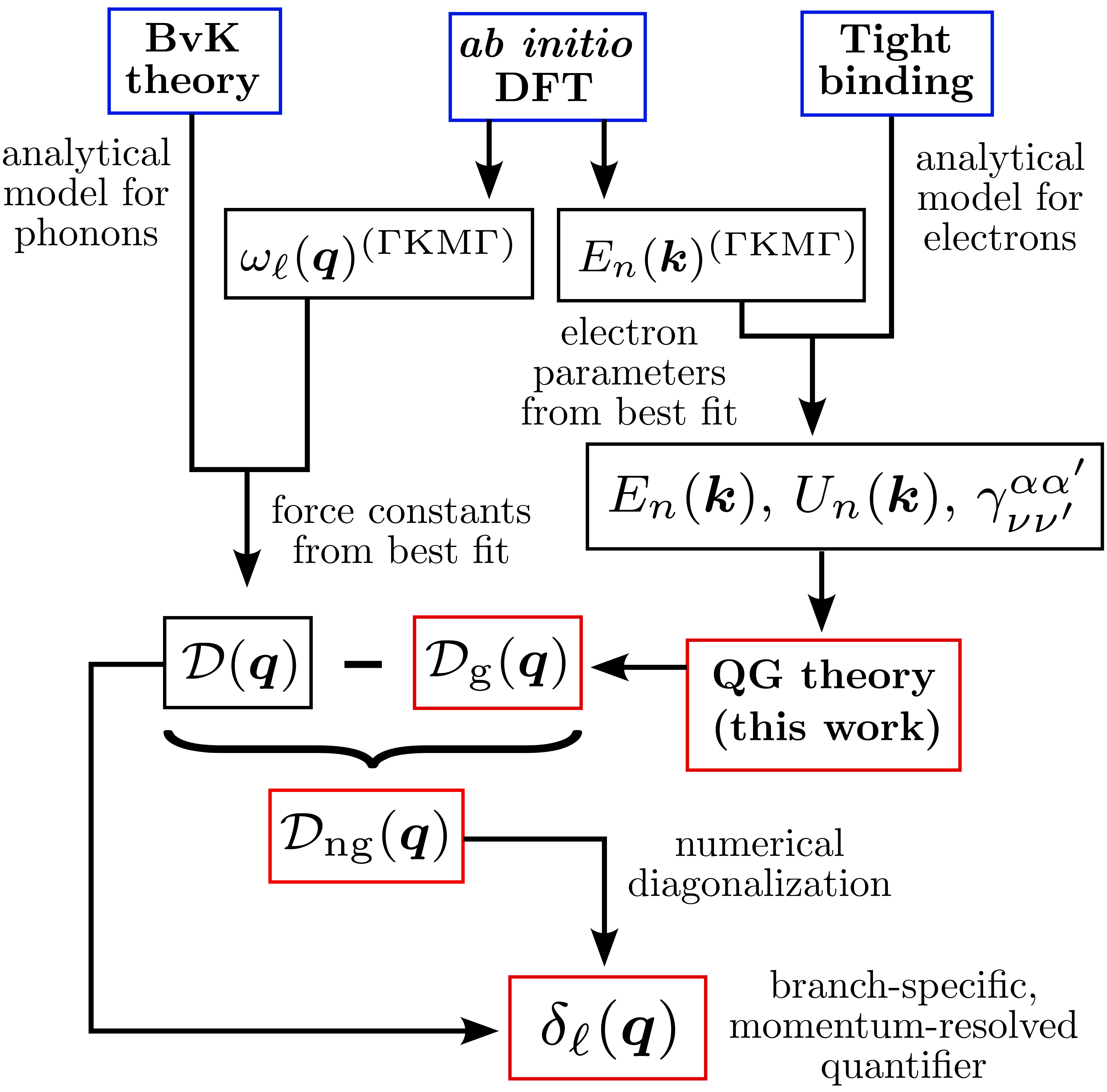
Figure 2: (Color online) Workflow followed for the case of graphene. The same method can be applied to any material for which the relevant hopping integrals are well-described by the GA. Fitting the BvK model to ab initio data on the high-symmetry line $\Gamma$KM$\Gamma$ allows us to extract the force constants and thus calculate the DM on the entire FBZ. The same fitting procedure is followed in order to obtain all the relevant information on electrons, thus allowing us to calculate the geometric contribution to the DM ${\cal D}_{\rm g}(\bm{q})$ and the momentum-resolved quantifier $\delta_{\ell}(\bm{q})$ of quantum geometry on the phonon spectra.

Within the GA, we are able to neatly separate the geometric contribution to the electronic force constants (13). We start from the Fourier transforms of the hopping matrix and of its derivatives, i.e. $h(\bm{k})=\sum_{p}e^{-i\bm{k}\cdot(\bm{R}_{p}+\bm{\tau}_{\nu}-\bm{\tau}_{\nu^{\prime}})}\left.t(\bm{r})\right|_{\bm{R}_{p}+\bm{\tau}_{\nu}-\bm{\tau}_{\nu^{\prime}}}$, $f_{i}(\bm{k})=\sum_{p}e^{-i\bm{k}\cdot(\bm{R}_{p}+\bm{\tau}_{\nu}-\bm{\tau}_{\nu^{\prime}})}\left.\partial_{r_{i}}t(\bm{r})\right|_{\bm{R}_{p}+\bm{\tau}_{\nu}-\bm{\tau}_{\nu^{\prime}}}$ and $M_{ij}(\bm{k})=\sum_{p}e^{-i\bm{k}\cdot(\bm{R}_{p}+\bm{\tau}_{\nu}-\bm{\tau}_{\nu^{\prime}})}\partial_{r_{i}r_{j}}^{2}\left.t(\bm{r})\right|_{\bm{R}_{p}+\bm{\tau}_{\nu}-\bm{\tau}_{\nu^{\prime}}}$. The key property of the GA is that the following identities hold true [65]: $\partial_{r_{i}}t(\bm{r})=\gamma r_{i}\,t(\bm{r})$ and $\partial^{2}_{r_{i}r_{j}}t(\bm{r})=(\gamma\delta_{ij}+\gamma^{2}r_{i}r_{j})\,t(\bm{r})$. We therefore find the following results, which are valid in the framework of the GA:

$$f_{i}(\bm{k}) =i\gamma\partial_{k_{i}}h(\bm{k})~,$$ (23)

$$M_{ij}(\bm{k}) =\big{(}\gamma\delta_{ij}-\gamma^{2}\partial_{k_{i}k_{j}}^{2}\big{)}h(\bm{k})~.$$ (24)

The Bloch Hamiltonian $h(\bm{k})$ defines both the energy bands $E_{n}(\bm{k})$ and the Bloch eigenvectors $U_{n}(\bm{k})$ via the eigenvalue equation $h(\bm{k})U_{n}(\bm{k})=E_{n}(\bm{k})U_{n}(\bm{k})$, thus providing the following explicit form $P_{n}(\bm{k})=U_{n}(\bm{k})U_{n}^{\dagger}(\bm{k})$ for the projection matrices. Identities (23) and (24), together with the spectral decomposition $h(\bm{k})=\sum_{n}E_{n}(\bm{k})P_{n}(\bm{k})$, allow us to decompose $f_{i}(\bm{k})$ and $M_{ij}(\bm{k})$ into dispersive (or energetic) and geometric parts. For $f_{i}(\bm{k})$, we have $f_{i}(\bm{k})=f_{i}^{\rm E}(\bm{k})+f_{i}^{\rm g}(\bm{k})$, with

$$f_{i}^{\rm E}(\bm{k}) =i\gamma\sum_{n}\partial_{k_{i}}E_{n}(\bm{k})P_{n}(\bm{k})~,$$ (25)

$$f_{i}^{\rm g}(\bm{k}) =i\gamma\sum_{n}E_{n}(\bm{k})\partial_{k_{i}}P_{n}(\bm{k})~.$$ (26)

The quantity $f_{i}^{\rm g}(\bm{k})$ is the geometric contribution to $f_{i}(\bm{k})$ [56], since it arises due to the momentum dependence of $P_{n}(\bm{k})$ and is zero in the case of trivial geometry. The term $f_{i}^{\rm E}(\bm{k})$, on the other hand, is a dispersive term, as it scales with the group velocity and is zero in the case of a perfectly flat band. The Fourier transform $M_{ij}(\bm{k})$ of the Hessian tensor is decomposed in the same fashion, as shown in detail in App. VII. While the geometric nature of the gradient $f_{i}(\bm{k})$ of the Bloch Hamiltonian has been discussed at length in Ref. [56]—where it was shown that $f_{i}(\bm{k})$ controls the strength of the EPI—in this work we deal with higher-order contributions contained in the Hessian tensor $M_{ij}(\bm{k})$, which scale as the second-order derivatives $\partial_{k_{i}}\partial_{k_{j}}P_{n}(\bm{k})$ of the projection matrix. While these are obviously recognizable as non-trivial geometric terms, they do not enter the QGT. This suggests the intriguing possibility that higher-order geometric structures have a role in defining the properties of crystals.

The purely electronic contribution to the force-constant matrix in Eq. (13) is a function of Hamiltonian derivatives only. Inserting the different contributions (25)-(26) to $f_{i}(\bm{k})$ into Eqs. (14)-(15) and doing the same for $M_{ij}(\bm{k})$, we can decompose the purely electronic part of the DM, ${\cal D}^{\rm(el)}(\bm{q})$, which has been introduced immediately after Eq. (9) into the sum of non-geometric and geometric contributions: ${\cal D}^{\rm(el)}(\bm{q})={\cal D}^{\rm(el)}_{\rm ng}(\bm{q})+{\cal D}_{\rm g}(\bm{q})$. Here, ${\cal D}_{\rm g}(\bm{q})$ is the non-trivial geometric contribution to the DM, which is solely of electronic nature and therefore has no ionic contribution, while ${\cal D}^{\rm(el)}_{\rm ng}(\bm{q})$ is that part of the electronic term in the DM which would be non-zero also in the case of a trivial quantum geometry. The entire DM can thus be decomposed as

$${\cal D}(\bm{q})={\cal D}_{\rm ng}(\bm{q})+{\cal D}_{\rm g}(\bm{q})~,$$ (27)

where ${\cal D}_{\rm ng}(\bm{q})\equiv{\cal D}^{\rm(ion)}(\bm{q})+{\cal D}_{\rm ng}^{\rm(el)}(\bm{q})$. Explicit expressions for the geometric contribution ${\cal D}_{\rm g}(\bm{q})$ to the DM can be found in App. VII.

The ability to identify the geometric contribution ${\cal D}_{\rm g}(\bm{q})$ to the DM allows us to define a momentum-resolved quantifier $\delta_{\ell}({\bm{q}})$ of quantum geometry in the phonon dispersion with the following procedure. First, we solve the secular problem defined by the Hermitian matrix ${\cal D}_{\rm ng}(\bm{q})$, i.e.

$$\sum_{\nu^{\prime}j}\left[{\cal D}_{\rm ng}(\bm{q})\right]_{\nu i}^{\nu^{\prime}j}\tilde{w}^{(\ell)}_{\nu^{\prime}j}(\bm{q})=\tilde{\omega}_{\ell}^{2}(\bm{q})\,\tilde{w}_{\nu i}^{(\ell)}(\bm{q})~.$$ (28)

For each phonon branch, defined by the label $\ell$, and phonon momentum $\bm{q}$, we consider the relative deviation $\delta_{\ell}(\bm{q})$ of $\tilde{\omega}_{\ell}(\bm{q})$ from the real phonon dispersion $\omega_{\ell}({\bm{q}})$—i.e. the phonon dispersion calculated with the full dynamical matrix as in Eq. (8)—thus defining:

$$\delta_{\ell}(\bm{q})\equiv\frac{\tilde{\omega}_{\ell}(\bm{q})-\omega_{\ell}(\bm{q})}{\tilde{\omega}_{\ell}(\bm{q})}~.$$ (29)

The quantifier $\delta_{\ell}(\bm{q})$ can be interpreted as a branch-specific, momentum-resolved indicator of how strong the ion motion couples to the quantum-geometric degrees of freedom of the electrons. While the dimensionless electron-phonon coupling [56] is just a number, $\delta_{\ell}(\bm{q})$ provides information about the role of quantum geometry on phonons throughout the FBZ.

Graphene as a case study.—The calculation of the geometric contribution to the phonons in graphene proceeds as schematized in Fig. 2. The DM is calculated analytically within a next-nearest-neighbor (NNN) BvK model [66], leaving the force constants as free parameters. The force constants are then determined by fitting the analytical results to ab initio density functional perturbation theory (DFPT) [67] calculations along the high-symmetry $\Gamma$KM$\Gamma$ path. Details on the ab initio calculations can be found in App. VIII and Refs. [68, 69, 70, 71, 72, 73, 74, 75, 76].

\begin{overpic}[width=216.81pt]{figures/fig3a.png} \put(7.0,140.0){\rm{(a)}} \end{overpic}

\begin{overpic}[width=216.81pt]{figures/fig3b.png} \put(7.0,140.0){\rm{(b)}} \end{overpic}

Figure 3: (Color online) (a) Momentum-resolved quantifier $\delta_{\ell}(\bm{q})$ as defined in Eq. (29) for the transverse (blue squares) and longitudinal (purple circles) acoustic phonon modes in graphene, evaluated along the high-symmetry contour shown in the inset of Fig 1. (b) Same as in panel (a), but for the transverse and longitudinal optical phonon modes.

The electronic Hamiltonian is calculated analytically by using a linear combination of atomic orbitals (LCAO) within the next-next-nearest-neighbor (NNNN) tight-binding approximation, leaving hopping and overlap integrals as free parameters [77]. These are in turn determined by fitting the analytical model to ab initio density functional theory (DFT) data on the $\Gamma$KM$\Gamma$ high-symmetry path. This allows us to reconstruct the Hamiltonian on the full FBZ, thus obtaining, by means of numerical diagonalization, all the information on the $\pi$ bands and their geometric structure, i.e. the energy bands $E_{\pm}(\bm{k})$ and the Bloch eigenvectors $U_{\pm}(\bm{k})$, where the subscript $+$ ($-$) denotes the conduction (valence) band. Only these two bands are considered in this calculation, as the hopping integrals that generate them are very well-described by the GA, as shown in App. VIII. We therefore fix $\alpha=\alpha^{\prime}=p_{z}$ and omit orbital labels from here on. The spatial dependence of $t_{AA}(\bm{r})$ and $t_{AB}(\bm{r})$, where $A$ and $B$ are sublattice labels, is obtained by repeating the best-fit procedure to determine the hopping integrals on a strained lattice, i.e. a graphene lattice on which a lattice constant different from that of the relaxed structure has been imposed.

Before presenting our main numerical results, we need to discuss the peculiarities of quantum geometry in graphene. The relevant quantum number in this material is the sublattice label, usually referred to as pseudospin [78]. Bloch states corresponding to the $\pi$ bands at a fixed wavevector $\bm{k}$ are obtained by producing a linear combination of states localized on the $A$ and $B$ sublattices. Thanks to this superposition, quantum geometry in graphene is non-trivial [27]. However, the singularity in the energy gradient at the location of the Dirac points—i.e. at the ${\bm{K}}$ and ${\bm{K}}^{\prime}$ points in the FBZ—translates into an infrared singularity in the $\bm{k}$-derivatives of the projection matrices, namely $\bm{\nabla}_{\bm{k}}P_{n}(\bm{k})\sim 1/k$, so the QGT (21) is ill-defined. In order to correct this behavior, we propose to use a natural regularization by shifting the energy of $p_{z}$ orbitals localized on $A$-type sublattice sites by a small amount $\Delta$ with respect to that of the $B$-type sublattice sites. This staggered potential breaks inversion symmetry (as in the case of graphene aligned to hBN [79]) and opens a gap $\Delta$ between the two $\pi$ bands, generating a finite Semenoff mass [78]. The trace of the Fubini-Study metric and the Berry curvature for a Semenoff-gapped graphene are shown in App. VIII. We emphasize that this regularization is not needed in the theory of the quantum geometric contribution to the EPI [56] because, by definition, the electron-phonon coupling constant $\lambda$ does not depend on integrals over the Fermi sea but, rather, only on integrals over the Fermi surface. In order to obtain the numerical results reported in Fig. 1 and Fig. 3, a gap $\Delta=1~{\rm meV}$ has been used for the regularization of the QGT. We have checked that the gap in the LA/TA modes is independent of the value of the Semenoff mass for $\Delta\lesssim 100~{\rm meV}$, as shown in App. VIII. Additional information on the application of our theory to graphene can be found in the latter, while analytical calculations for massless Dirac fermions ($\Delta=0$) are reported in App. IX.

Discussion.—Our main numerical results for $\omega_{\ell}(\bm{q})$, $\tilde{\omega}_{\ell}(\bm{q})$, and $\delta_{\ell}(\bm{q})$ for the case of in-plane phonons in graphene are illustrated in Figs. 1 and 3. (The role of quantum geometry on out-of-plane flexural phonons [78] is well beyond the scope of the present theory, which is strictly 2D.) As one could have guessed a priori, the removal of the geometric contribution does not tamper with the symmetries of the system. As a consequence, the degeneracy of the $\tilde{\omega}_{{\rm LO},{\rm TO}}({\bm{q}})$ modes at the $\Gamma$ point [80] is preserved. For these modes, $\delta_{{\rm LO},{\rm TO}}({\bm{q}})$ is at most $14\%$ at the zone center—see Fig. 3(b).

Removing the quantum geometric contribution from the DM has instead a remarkable qualitative implication on acoustic phonons. Indeed, as we clearly see in Fig. 1, the TA and LA phonon dispersions $\tilde{\omega}_{\ell}({\bm{q}})$ calculated without geometric contribution to the DM are gapped at the zone center, i.e. $\tilde{\omega}_{\rm LA,\,TA}({\bm{q}}={\bm{0}})\approx 40~{\rm meV}$. In this case, the dimensionless quantifier $\delta_{{\rm LA},{\rm TA}}({\bm{q}})$ reaches the value of $100\%$ at the zone center—see Fig. 3(a).

This result is truly significant in light of the fact that the removal of the geometric contribution ${\cal D}_{\rm g}(\bm{q})$ from the full DM ${\cal D}(\bm{q})$ does not imply neither the breaking of discrete lattice symmetries nor time reversal. What is the mechanism behind the gap opening in the LA/TA modes represented by blue crosses in Fig. 1? The key point is that the full electronic DM ${\cal D}^{\rm(el)}(\bm{q})$, comprising both the trivial contribution and the quantum geometric one, satisfies the acoustic sum rule (12). As stated above, the latter is responsible, together with Eq. (11), for the gapless nature of the LA/TA branches. Removing the geometric contribution from ${\cal D}^{\rm(el)}(\bm{q})$ leads to a violation of the acoustic sum rule (12). This is the origin of the gap opening in the LA/TA branches in Fig. 1. Our results therefore show that the Goldstone theorem is violated if one neglects the quantum geometric contribution to the DM, inherited by the geometric properties of Bloch electrons.

Acknowledgments.—G. P. and M. P. wish to thank Angelo Esposito for useful and inspiring discussions. This work was supported by the MUR - Italian Ministry of University and Research under the “Research projects of relevant national interest - PRIN 2020” - Project No. 2020JLZ52N (“Light-matter interactions and the collective behavior of quantum 2D materials, q-LIMA”) and by the European Union under grant agreements No. 101131579 - Exqiral and No. 873028 - Hydrotronics. Views and opinions expressed are however those of the author(s) only and do not necessarily reflect those of the European Union or the European Commission. Neither the European Union nor the granting authority can be held responsible for them. B.A.B. and H.H. were supported by the Gordon and Betty Moore Foundation through Grant No. GBMF8685 towards the Princeton theory program, the Gordon and Betty Moore Foundation’s EPiQS Initiative (Grant No. GBMF11070), the Office of Naval Research (ONR Grant No. N00014-20-1-2303), the Global Collaborative Network Grant at Princeton University, the Simons Investigator Grant No. 404513, the BSF Israel US foundation No. 2018226, the NSF-MERSEC (Grant No. MERSEC DMR 2011750), the Simons Collaboration on New Frontiers in Superconductivity (Grant No. SFI-MPS-NFS-00006741-01), and the Schmidt Foundation at the Princeton University. Y.J. was supported by the European Research Council (ERC) under the European Union’s Horizon 2020 research and innovation program (Grant Agreement No. 101020833), as well as by the IKUR Strategy under the collaboration agreement between Ikerbasque Foundation and DIPC on behalf of the Department of Education of the Basque Government.

This Supplemental Material is organized into nine Appendices. In App. I, we briefly present some fundamental identities regarding the QGT in a crystal. In App. II, we give a proof of the acoustic sum rules for the interatomic force constants. In App. III, we show how to write the electronic part of the force-constant matrix in terms of derivatives of the electronic Hamiltonian only. In App. IV we find explicit, general analytical formulas for the electronic part of the dynamical matrix of a crystal. App. V contains details on the construction of the formal analogy between phonon theory and linear response theory. In App. VI, we verify the TRK sum rule for a simple 1D toy model. App. VII is devoted to the isolation of nontrivial geometric terms in the dynamical matrix. In App. VIII, we discuss details of the application of the theory to graphene. Finally, in App. IX, we calculate analytically the diagonal terms in ${\cal D}^{(2)}_{\rm g}(\bm{0})$ for the case of massless Dirac fermions.

Appendix I The Quantum Geometric Tensor in solid-state systems

The problem of electrons in a periodic potential is described by the Hamiltonian

$$\hat{{\cal H}}_{\rm e}=\frac{\hat{\bm{p}}^{2}}{2m_{\rm e}}+\hat{V}(\bm{r})\qquad{\rm with}\qquad\hat{V}(\bm{r}+\bm{R}^{0}_{p\nu})=\hat{V}(\bm{r})~,$$ (1)

where we have used the same notation for the lattice structure as in the main text. The eigenstates $\psi_{n\bm{k}}(\bm{r})$ of the Hamiltonian (1) are of the Bloch type [1], i.e. $\psi_{n\bm{k}}(\bm{r})=e^{i\bm{k}\cdot\hat{\bm{r}}}u_{n\bm{k}}(\bm{r})$, with $u_{n\bm{k}}(\bm{r})=u_{n\bm{k}}(\bm{r}+\bm{R}^{0}_{p\nu})$. They are labelled by a discrete band number $n$ and depend parametrically on the Bloch quasi-momentum $\bm{k}\in{\rm FBZ}$. The crystal is therefore described by the Hamiltonian $\hat{{\cal H}}_{\rm e}$ which does not explicitly depend on the Bloch quasi-momentum, with boundary conditions that do depend on it. To transition to a formulation where the boundary conditions remain $\bm{k}$-independent while the Hamiltonian retains its $\bm{k}$-dependence, it is useful to apply a momentum shift [2]:

$$\hat{\cal H}_{\rm e}\to\hat{{\cal H}}_{\rm e}(\bm{k})\equiv e^{-i\bm{k}\cdot\hat{\bm{r}}}\,\hat{{\cal H}}_{\rm e}\,e^{i\bm{k}\cdot\hat{\bm{r}}}=\frac{{(\hat{\bm{p}}+\hbar\bm{k})}^{2}}{2m_{\rm e}}+\hat{V}(\bm{r})~.$$ (2)

The eigenstates of the Hamiltonian (2) reduce from being of the Bloch type to being only the periodic part of the Bloch wavefunction, i.e. they coincide with the quantity $u_{n\bm{k}}(\bm{r})$. This representation is well-suited to discuss topology and, more in general, quantum geometry.

As stated in the main text, in the case in which bands do not touch, the analysis of the geometry of wavefunctions requires the definition of a different QGT for each band [3]:

$$\mathcal{Q}^{(n)}_{ij}(\bm{k})=\operatorname{Tr}\left\{\partial_{k_{i}}\hat{P}_{n}(\bm{k})\left[1-\hat{P}_{n}(\bm{k})\right]\partial_{k_{j}}\hat{P}_{n}(\bm{k})\right\}~,$$ (3)

where $\hat{P}_{n}(\bm{k})\equiv|u_{n\bm{k}}\rangle\langle u_{n\bm{k}}|$ is the projection operator on the state $|u_{n\bm{k}}\rangle$. The expression (3) of the QGT is appropriate for numerical calculations, as it does not require any type of gauge smoothing. Indeed, the projectors $\hat{P}_{n}(\bm{k})$ are manifestly gauge-invariant. We note that, due to the presence of a Semenoff mass $\Delta$ acting as a regularizer in our description of the quantum geometry of graphene, we do not need to deal with band crossings.

We now show that the definition (3) is equivalent to the original definition provided by Provost and Vallee [4] and given in Eqs. (1)-(Phonon spectra, quantum geometry, and the Goldstone theorem) of the main text. We begin by transforming the projector-based expression (3) into a formulation that explicitly incorporates an exact eigenstate representation:

$$\mathcal{Q}^{(n)}_{ij}(\bm{k}) =\operatorname{Tr}\{\partial_{k_{i}}\Bigl{[}|u_{n\bm{k}}\rangle\langle u_{n\bm{k}}|\Bigr{]}\Bigl{[}1-|u_{n\bm{k}}\rangle\langle u_{n\bm{k}}|\Bigr{]}\partial_{k_{j}}\Bigl{[}|u_{n\bm{k}}\rangle\langle u_{n\bm{k}}|\Bigr{]}\}$$

$$=\sum_{m}\langle u_{m\bm{k}}|\Bigl{[}|\partial_{k_{i}}u_{n\bm{k}}\rangle\langle u_{n\bm{k}}|+|u_{n\bm{k}}\rangle\langle\partial_{k_{i}}u_{n\bm{k}}|\Bigr{]}\Bigl{[}\sum_{l\neq n}|u_{l\bm{k}}\rangle\langle u_{l\bm{k}}|\Bigr{]}\Bigl{[}|\partial_{k_{j}}u_{n\bm{k}}\rangle\langle u_{n\bm{k}}|+|u_{n\bm{k}}\rangle\langle\partial_{k_{j}}u_{n\bm{k}}|\Bigr{]}|u_{m\bm{k}}\rangle$$

$$=\sum_{m}\langle u_{m\bm{k}}|u_{n\bm{k}}\rangle\langle\partial_{k_{i}}u_{n\bm{k}}|\Bigl{[}\sum_{l\neq n}|u_{l\bm{k}}\rangle\langle u_{l\bm{k}}|\Bigl{]}|\partial_{k_{j}}u_{n\bm{k}}\rangle\langle u_{n\bm{k}}|u_{m\bm{k}}\rangle$$

$$=\sum_{m}\delta_{mn}\langle\partial_{k_{i}}u_{n\bm{k}}|\Bigl{[}\sum_{l\neq n}|u_{l\bm{k}}\rangle\langle u_{l\bm{k}}|\Bigr{]}|\partial_{k_{j}}u_{n\bm{k}}\rangle\delta_{nm}$$

$$=\bigl{\langle}\partial_{k_{i}}u_{n\bm{k}}|\partial_{k_{j}}u_{n\bm{k}}\bigr{\rangle}-\bigl{\langle}\partial_{k_{i}}u_{n\bm{k}}|u_{n\bm{k}}\bigr{\rangle}\bigl{\langle}u_{n\bm{k}}|\partial_{k_{j}}u_{n\bm{k}}\bigr{\rangle}~.$$ (4)

Here, we used the completeness relation $\sum_{n}|u_{n\bm{k}}\rangle\langle u_{n\bm{k}}|=\openone$ and orthogonality of the eigenstates, i.e. $\langle u_{n\bm{k}}|u_{m\bm{k}}\rangle=\delta_{nm}$, which are both valid at each fixed value of $\bm{k}$, as well as the definition of the trace on the parametric Hilbert space, $\operatorname{Tr}[\cdots]=\sum_{m}\langle u_{m\bm{k}}|\cdots|u_{m\bm{k}}\rangle$, again valid at each fixed value of ${\bm{k}}$.

We now note that the second term in the last line of Eq. (I) is real. We therefore have:

$$\operatorname{Re}\mathcal{Q}^{(n)}_{ij}(\bm{k}) = \operatorname{Re}\Bigl{[}\bigl{\langle}\partial_{k_{i}}u_{n\bm{k}}|\partial_{k_{j}}u_{n\bm{k}}\bigr{\rangle}\Bigr{]}-\bigl{\langle}\partial_{k_{i}}u_{n\bm{k}}|u_{n\bm{k}}\bigr{\rangle}\bigl{\langle}u_{n\bm{k}}|\partial_{k_{j}}u_{n\bm{k}}\bigr{\rangle}~,$$ (5a)

$$2i\operatorname{Im}\mathcal{Q}^{(n)}_{ij}(\bm{k}) = \mathcal{Q}^{(n)}_{ij}(\bm{k})-\bigl{[}\mathcal{Q}^{(n)}_{ij}(\bm{k})\bigr{]}^{*}=\bigl{\langle}\partial_{k_{i}}u_{n\bm{k}}|\partial_{k_{j}}u_{n\bm{k}}\bigr{\rangle}-\bigl{\langle}\partial_{k_{j}}u_{n\bm{k}}|\partial_{k_{i}}u_{n\bm{k}}\bigr{\rangle}~.$$ (5b)

By substituting $|u_{n\bm{k}}\rangle\leftrightarrow|\psi_{\bm{k}}\rangle$, we see that Eqs. (5a) and (5b) coincide with the definitions of $g_{ij}(\bm{k})$ and ${\cal F}_{ij}(\bm{k})$ given in Eqs. (2) and (Phonon spectra, quantum geometry, and the Goldstone theorem)of the main text, respectively.

The form given in Eq. (3), however, is not quite equivalent to that provided in Eq. (21) of the main text: the formal correspondence $\hat{P}_{n}(\bm{k})\to P_{n}(\bm{k})\equiv U_{n}(\bm{k})U_{n}^{\dagger}(\bm{k})$ between the projection operator and the projection matrix is only valid under the tight-binding approximation, within which all the information on the $\bm{k}$-dependence of the Bloch eigenstates $|u_{n\bm{k}}\rangle$ is contained in the Bloch eigenvector $U_{n}(\bm{k})$. A proof of this statement can be found in the Supplementary information of Ref. [5].

Appendix II Proof of the acoustic sum rules

We start by proving the acoustic sum rule for the complete dynamical matrix and for the ionic and electronic contributions to it. It is sufficient to impose invariance of the interatomic potential energy $V(\{\bm{u}_{p\nu}\})$ felt by each atom under a global translation of the entire crystal by a constant vector $\bm{b}$. Let us calculate the potential energy felt by an atom in the $p=0$ unit cell, with basis vector $\bm{\tau}_{\nu}$:

$$V(\bm{u}_{0\nu})=\sum_{p^{\prime}}\sum_{\nu^{\prime}}u_{0\nu i}\,\bigl{[}{\cal C}\bigr{]}_{0\nu i}^{p^{\prime}\nu^{\prime}j}u_{p^{\prime}\nu^{\prime}j}=\sum_{p^{\prime}}\sum_{\nu^{\prime}}\bigl{(}u_{0\nu i}+b_{i}\bigr{)}\,\bigl{[}{\cal C}\bigr{]}_{0\nu i}^{p^{\prime}\nu^{\prime}j}\bigl{(}u_{p^{\prime}\nu^{\prime}j}+b_{j}\bigr{)}~,$$ (6)

implying

$$\sum_{p^{\prime}}\sum_{\nu^{\prime}}b_{i}\,\bigl{[}{\cal C}\bigr{]}_{0\nu i}^{p^{\prime}\nu^{\prime}j}b_{j}=0\qquad\forall~\bm{b}\in\mathds{R}^{D}~,$$ (7)

and therefore

$$\sum_{\nu^{\prime}}\sqrt{M_{\nu^{\prime}}}\bigl{[}{\cal D}(\bm{q}=\bm{0})\bigr{]}_{\nu i}^{\nu^{\prime}j}=\frac{1}{\sqrt{M_{\nu}}}\sum_{p^{\prime},\nu^{\prime}}\bigl{[}{\cal C}\bigr{]}_{0\nu i}^{p^{\prime}\nu^{\prime}j}=0\qquad\forall~\nu,i,j~.$$ (8)

The same line of reasoning can be applied to ${\cal D}^{(\rm ion)}(\bm{q}=\bm{0})$, substituting the interatomic potential with the bare Coulomb repulsive potential, and thus to the electronic contribution ${\cal D}^{(\rm el)}(\bm{q}=\bm{0})$.

Appendix III The force constants in terms of Hamiltonian derivatives

To derive an explicit expression for the quantity ${\cal C}^{\rm(el)}$ as defined in Eq. (7), we use the Hellmann-Feynmann theorem [6] carefully combined with the second-order derivative:

$$\bigl{[}{\cal C}^{\text{(el)}}\bigr{]}^{p^{\prime}\nu^{\prime}j}_{p\nu i} =\left.\frac{\partial^{2}}{\partial u_{p\nu i}\,\partial u_{p^{\prime}\nu^{\prime}j}}\left\langle\phi^{(0)}_{\{\bm{u}_{p\nu}\}}\right|\hat{\cal H}_{\text{e}}(\{\bm{u}_{p\nu}\})\left|\phi^{(0)}_{\{\bm{u}_{p\nu}\}}\right\rangle\,\right|_{0}$$

$$=\left.\partial_{p\nu i}\left\langle\phi^{(0)}\right|\partial_{p^{\prime}\nu^{\prime}j}\hat{\cal H}_{\text{e}}\left|\phi^{(0)}\right\rangle\,\right|_{0}$$

$$=\left.\left\langle\partial_{p\nu i}\phi^{(0)}\right|\partial_{p^{\prime}\nu^{\prime}j}\hat{\cal H}_{\text{e}}\left|\phi^{(0)}\right\rangle\,\right|_{0}+\left.\left\langle\phi^{(0)}\right|\partial_{p^{\prime}\nu^{\prime}j}\hat{\cal H}_{\text{e}}\left|\partial_{p\nu i}\phi^{(0)}\right\rangle\,\right|_{0}$$

$$\,+\left.\left\langle\phi^{(0)}\right|\partial_{p\nu i}\partial_{p^{\prime}\nu^{\prime}j}\hat{\cal H}_{\text{e}}\left|\phi^{(0)}\right\rangle\,\right|_{0}~.$$ (9)

Here, we used the shorthand notation $\partial_{p\nu i}\equiv\partial/\partial u_{p\nu i}$ and omitted, starting from the second equality, the explicit parametric dependence of the Hamiltonian and its ground state on $\{\bm{u}_{p\nu}\}$.

Unfortunately, the parametric derivatives of the many-body ground state in the previous expression are unpractical formal expressions because there is no simple way to compute them. We therefore choose to eliminate them in favor of derivatives of the Hamiltonian. However, this comes at the cost of introducing the exact excited eigenstates of the Hamiltonian, which are defined by the Schrödinger equation:

$$\hat{\cal H}_{\text{e}}|{\phi^{(m)}}\rangle=\mathcal{E}_{m}|{\phi^{(m)}}\rangle~.$$ (10)

We then exploit the Epstein generalization [1] of the Hellmann-Feynman theorem:

$$\left|\partial_{p\nu i}\phi^{(0)}\right\rangle=\sum_{m\neq 0}\left|\phi^{(m)}\right\rangle\frac{\left\langle\phi^{(m)}\left|\partial_{p\nu i}\hat{\cal H}_{\text{e}}\right|\phi^{(0)}\right\rangle}{\mathcal{E}_{0}-\mathcal{E}_{m}}~.$$ (11)

Using Eq. (11) inside Eq. (III), we immediately obtain Eqs. (14)-(15) of the main text.

Appendix IV Formulas for the dynamical matrix

The amplitudes $\left\langle\phi^{(m)}_{\{\bm{0}\}}\middle|\partial_{p\nu i}\hat{\cal H}_{\rm e}\middle|\phi^{(0)}_{\{\bm{0}\}}\right\rangle$ appearing in Eq. (14) of the main text are nonzero only for the following class of states:

$$|{\phi^{(n\bm{k},\,n^{\prime}\bm{k}^{\prime})}_{\{\bm{0}\}}}\rangle=\hat{\gamma}_{n^{\prime}\bm{k}^{\prime}}^{\dagger}\hat{\gamma}_{n\bm{k}\vphantom{{}^{\prime}}}^{\vphantom{\dagger}}\left|\phi^{(0)}_{\{\bm{0}\}}\right\rangle~,\qquad\text{with}\qquad\begin{cases}E_{n}(\bm{k})<\mu\\ E_{n^{\prime}}(\bm{k}^{\prime})>\mu\end{cases}~,$$ (12)

where $\mu$ is the chemical potential.

The first derivatives of the Hamiltonian with respect to the displacements, which appear in Eq. (14) of the main text, can be calculated starting from the modified tight-binding Hamiltonian—see Eq. (4) of the main text. The evaluation of these derivatives on the states (12) allows us to get to an explicit form for the term ${\cal C}^{(\rm{el,\,1})}$ as defined in Eq. (14). The expectation value on the Fermi sea that appears in the Eq. (15) for $\bigl{[}{\cal C}^{(\rm{el,\,2})}_{ij}\bigr{]}^{pp^{\prime}}_{\nu\nu^{\prime}}$ in the main text is evaluated by explicit calculation of the second derivatives of the Hamiltonian with respect to the displacements. By taking the Fourier transform with respect to the ion positions, thereby defining

$$\bigl{[}{\cal D}^{\rm(el,\,1/2)}(\bm{q})\bigr{]}_{\nu i}^{\nu^{\prime}j}\equiv\frac{1}{\sqrt{M_{\nu\vphantom{{}^{\prime}}}M_{\nu^{\prime}}}}\sum_{p}e^{-i\bm{q}\cdot(\bm{R}_{p}+\bm{\tau}_{\nu\vphantom{{}^{\prime}}}-\bm{\tau}_{\nu^{\prime}})}\,\bigl{[}{\cal C}^{\rm(el,\,1/2)}_{ij}\bigr{]}^{p,p^{\prime}=0}_{\nu\nu^{\prime}}$$ (13)

so that ${\cal D}^{\rm(el)}(\bm{q})={\cal D}^{\rm(el,\,1)}(\bm{q})+{\cal D}^{\rm(el,\,2)}(\bm{q})$, we obtain the following explicit formulas for the dynamical matrix:

$$\bigl{[}{\cal D}^{\rm(el,\,1)}(\bm{q})\bigr{]}_{\nu i}^{\nu^{\prime}j}=\frac{1}{\sqrt{M_{\nu}M_{\nu^{\prime}}}}\,\frac{2}{N}\sum_{n}^{\rm occ.}\sum_{n^{\prime}}^{\rm unocc.}\sum_{\bm{k}}^{\text{FBZ}}\left\{\frac{\bigl{[}F_{i}(n\bm{k},n^{\prime}\bm{k}+\bm{q})\bigr{]}_{\nu}\bigl{[}F_{j}(n^{\prime}\bm{k}+\bm{q},n\bm{k})\bigr{]}_{\nu^{\prime}}}{E_{n}(\bm{k})-E_{n^{\prime}}(\bm{k}+\bm{q})}+{\rm H.c.}\right\}$$ (14)

and

$$\bigl{[}{\cal D}^{\rm(el,\,2)}(\bm{q})\bigr{]}_{\nu i}^{\nu^{\prime}j}=\frac{1}{\sqrt{M_{\nu}M_{\nu^{\prime}}}}\,\frac{2}{N}\sum_{\tilde{\nu}}\sum_{n}^{\rm occ.}\sum_{\bm{k}\tilde{\bm{k}}}^{\text{FBZ}}\sum_{\alpha\alpha^{\prime}}\left[\delta_{\nu\nu^{\prime}}\delta_{\tilde{\bm{k}},\,\bm{0}}-\delta_{\tilde{\nu}\nu^{\prime}}\delta_{\tilde{\bm{k}},\,\bm{q}}\right]\left\{\bigl{[}M_{ij}(\bm{k}+\tilde{\bm{k}})\bigr{]}_{\nu\alpha}^{\tilde{\nu}\alpha^{\prime}}\bigl{[}P_{n}(\bm{k})\bigr{]}_{\tilde{\nu}\alpha^{\prime}}^{\nu\alpha}+\rm{H.c.}\right\}~,$$ (15)

where $P_{n}(\bm{k})=U_{n}(\bm{k})U^{\dagger}_{n}(\bm{k})$ is the projection matrix onto the eigenvector $U_{n}(\bm{k})$ of the Bloch Hamiltonian $h(\bm{k})$, while $N$ is the number of atoms in the Born-von Karman supercell, which is equal to the number of Bloch wavevectors involved in the sum over the first Brillouin zone (FBZ). In writing Eqs. (14)-(15) we employed the following shorthand notation for summations over the Fermi sea,

$$\sum_{nn^{\prime}}\sum_{\bm{k}\bm{k}^{\prime}}^{\text{FBZ}}\Theta\bigl{(}\mu-E_{\nu}(\bm{k})\bigr{)}\,\Theta\bigl{(}E_{n^{\prime}}(\bm{k}^{\prime})-\mu\bigr{)}=\sum_{\bm{k}\in\text{FBZ}}^{E_{n}(\bm{k})<\mu}\sum_{\bm{k}^{\prime}\in\text{FBZ}}^{E_{\nu^{\prime}}(\bm{k}^{\prime})>\mu}\equiv\sum_{n\bm{k}}^{\rm occ.}\sum_{n^{\prime}\bm{k}^{\prime}}^{\rm unocc.}~,$$ (16)

and defined the following quantity:

$$\bigl{[}F_{i}(n\bm{k},n^{\prime}\bm{k}^{\prime})\bigr{]}_{\nu}\equiv\sum_{\tilde{\nu}}\sum_{\nu_{1}\nu_{2}}\sum_{\alpha\alpha^{\prime}}\bigl{[}U^{\dagger}_{n}(\bm{k})\bigr{]}_{\nu_{1}\alpha}\biggl{\{}\delta_{\nu\nu_{1}}\delta_{\tilde{\nu}\nu_{2}}\bigl{[}f_{i}(\bm{k}^{\prime})\bigr{]}_{\nu\alpha}^{\tilde{\nu}\alpha^{\prime}}-\delta_{\nu\nu_{2}}\delta_{\tilde{\nu}\nu_{1}}\bigl{[}f_{i}(\bm{k})]_{\tilde{\nu}\alpha}^{\nu\alpha^{\prime}}\biggr{\}}\bigl{[}U^{\vphantom{\dagger}}_{n^{\prime}}(\bm{k}^{\prime})\bigr{]}_{\nu_{2}\alpha^{\prime}}~.$$ (17)

Appendix V Formal analogy with linear response theory

The analogy with linear response theory is built as follows. The small-displacement expansion of the electronic Hamiltonian (Eq. (4) in the main text) is

$$\hat{{\cal H}}_{\bm{u}}=\left.\hat{{\cal H}}_{\bm{u}}\right|_{0}+\sum_{p,\nu,i}\left.\frac{\partial\hat{{\cal H}}_{\bm{u}}}{\partial u_{p\nu i}}\right|_{0}\,u_{p\nu i}+\frac{1}{2}\sum_{p,\nu,i}\sum_{p^{\prime}\nu^{\prime},j}\left.\frac{\partial^{2}\hat{{\cal H}}_{\bm{u}}}{\partial u_{p\nu i}\partial u_{p^{\prime}\nu^{\prime}j}}\right|_{0}\,u_{p\nu i}\,u_{p^{\prime}\nu^{\prime}j}~,$$ (18)

where we introduced the shorthand notation $\hat{{\cal H}}_{\bm{u}}\equiv\hat{\cal H}_{\rm e}(\{\bm{u}_{p\nu}\})$, and the $|_{0}$ subscript once again denotes the evaluation on the mechanical equilibrium configuration. The most general Hamiltonian of an electron system electron which has been minimally coupled to a time-independent gauge field $\bm{A}(\bm{r},t)=\bm{A}(\bm{r})$ is

$$\hat{\cal H}_{\bm{A}}=\left.\hat{\cal H}_{\bm{A}}\right|_{0}+\sum_{i}\int{\rm d}^{D}\bm{r}\,\left.\frac{\delta\hat{\cal H}_{\bm{A}}}{\delta A_{i}(\bm{r})}\right|_{{0}}\,A_{i}(\bm{r})+\frac{1}{2}\sum_{i,j}\iint{\rm d}^{D}\bm{r}\,{\rm d}^{D}\bm{r}^{\prime}\,\left.\frac{\delta^{2}\hat{\cal H}_{\bm{A}}}{\delta A_{i}(\bm{r})\delta A_{j}(\bm{r})}\right|_{0}\,A_{i}(\bm{r})A_{j}(\bm{r}^{\prime})~,$$ (19)

where $\delta$ denotes a functional derivative, and the $|_{0}$ subscript means $\bm{A}=0$. Considering a time-independent vector field parallels the Born-Oppenheimer approximation. The two expressions (18) and (19) are formally equivalent under exchange of

$$\bm{r}\leftrightarrow\bm{R}_{p\nu}~,\qquad\sum_{i}\int{\rm d}^{D}\bm{r}\leftrightarrow\sum_{i}\sum_{p,\,\nu}~,\qquad\hat{\cal H}_{\bm{A}}\leftrightarrow\hat{{\cal H}}_{\bm{u}}~,\qquad\bm{A}(\bm{r})\leftrightarrow\bm{u}_{p\nu}~,$$ (20)

Identifying $\bm{A}(\bm{r})$ with an electromagnetic vector potential, we can define the paramagnetic current operator $\hat{j}_{i}(\bm{r})$ and the diamagnetic operator $\hat{\cal T}_{ij}(\bm{r},\bm{r}^{\prime})$ respectively as

$$\hat{j}_{i}(\bm{r})\equiv\frac{c}{e}\left.\frac{\delta{\hat{\cal H}}_{\bm{A}}}{\delta A_{i}(\bm{r})}\right|_{0}~,$$ (21)

and

$$\hat{\cal T}_{ij}(\bm{r},\bm{r}^{\prime})\equiv\frac{c^{2}}{e^{2}}\left.\frac{\delta^{2}\hat{\cal H}_{\bm{A}}}{\delta A_{i}(\bm{r})\delta A_{j}(\bm{r}^{\prime})}\right|_{0}~.$$ (22)

The physical current operator for the Hamiltonian in Eq. (19) can be thus written as

$$\hat{J}_{i}(\bm{r})\equiv\frac{c}{e}\frac{\delta{\hat{\cal H}}_{\bm{A}}}{\delta A_{i}(\bm{r})}=\hat{j}_{p,i}(\bm{r})+\frac{e}{c}\sum_{j}\int{\rm d}^{D}\bm{r}^{\prime}\,\hat{\cal T}_{ij}(\bm{r},\bm{r}^{\prime})\,A_{j}(\bm{r}^{\prime})~.$$ (23)

By formal analogy, we can build the same operators for the theory described by the Hamiltonian (18):

$$\hat{j}_{p\nu i} \equiv\left.\frac{\partial\hat{{\cal H}}_{\bm{u}}}{\partial u_{p\nu i}}\right|_{0}~,$$ (24)

$$\hat{\cal T}_{p\nu i}^{p^{\prime}\nu^{\prime}j} \equiv\left.\frac{\partial^{2}\hat{{\cal H}}_{\bm{u}}}{\partial u_{p\nu i}\partial u_{p^{\prime}\nu^{\prime}j}}\right|_{0}~,$$ (25)

$$\hat{J}_{p\nu i} \equiv\hat{j}_{p\nu i}+\sum_{p^{\prime},\nu^{\prime},j}\hat{\cal T}_{p\nu i}^{p^{\prime}\nu^{\prime}j}u_{p^{\prime}\nu^{\prime}j}~.$$ (26)

For each of the two theories, we can build a zero-temperature, static, paramagnetic current-current response function, which can be written as follows in the Lehmann representation :

$$\chi_{j_{i}\,j_{j}}^{\vphantom{\dagger}}(\bm{r},\bm{r}^{\prime}) =\sum_{m\neq 0}\frac{\left\langle\phi^{(m)}_{\bm{A}=\bm{0}}\middle|\hat{j}_{i}(\bm{r})\middle|\phi^{(0)}_{\bm{A}=\bm{0}}\right\rangle\left\langle\phi^{(0)}_{\bm{A}=\bm{0}}\middle|\hat{j}_{j}(\bm{r}^{\prime})\middle|\phi^{(m)}_{\bm{A}=\bm{0}}\right\rangle}{{\cal E}_{0}-{\cal E}_{m}}+{\rm H.c.}~,$$ (27)

$$\chi_{j_{p\nu i}\,j_{p^{\prime}\nu^{\prime}j}}^{\vphantom{\dagger}} =\sum_{m\neq 0}\frac{\left\langle\phi^{(m)}_{\{\bm{0}\}}\middle|\hat{j}_{p\nu i}\middle|\phi^{(0)}_{\{\bm{0}\}}\right\rangle\left\langle\phi^{(0)}_{\{\bm{0}\}}\middle|\hat{j}_{p^{\prime}\nu^{\prime}j}\middle|\phi^{(m)}_{\{\bm{0}\}}\right\rangle}{{\cal E}_{0}-{\cal E}_{m}}+{\rm H.c.}~,$$ (28)

with the same notation for excited states of the Hamiltonian as in the main text. To obtain the electronic force constants, we start from Eq. (III), which states the following:

$$\bigl{[}{\cal C}^{\rm(el)}\bigr{]}_{p\nu i}^{p^{\prime}\nu^{\prime}j}=\left[\frac{\partial}{\partial u_{p^{\prime}\nu^{\prime}j}}\left\langle\phi^{(0)}_{\{\bm{u}_{p\nu}\}}\middle|\frac{\partial\hat{\cal H}_{\bm{u}}}{\partial u_{p\nu i}}\middle|\phi^{(0)}_{\{\bm{u}_{p\nu}\}}\right\rangle\right]_{0}\equiv\left[\frac{\partial}{\partial u_{p^{\prime}\nu^{\prime}j}}\left\langle\hat{J}_{p\nu i}\right\rangle\right]_{0}~,$$ (29)

where we introduced the shorthand notation $\langle\,\cdot\,\rangle\equiv\langle\phi^{(0)}_{\{\bm{u}_{p\nu}\}}|\cdot|\phi^{(0)}_{\{\bm{u}_{p\nu}\}}\rangle$. This equation parallels the definition of the physical current-current response function [6], i.e.

$$\chi^{J}_{ij}(\bm{r},\bm{r}^{\prime})\equiv\left[\frac{\delta}{\delta A_{j}(\bm{r}^{\prime})}\left\langle\phi^{(0)}_{\bm{A}}\middle|\frac{\delta\hat{\cal H}_{\bm{A}}}{\delta A_{i}(\bm{r})}\middle|\phi^{(0)}_{\bm{A}}\right\rangle\right]_{0}\equiv\left[\frac{\delta}{\delta A_{j}(\bm{r}^{\prime})}\left\langle\hat{J}_{i}(\bm{r})\right\rangle\right]_{0}~.$$ (30)

The expectation value of the physical current operator to first order in the gauge field amplitude is obtained as

$$\left\langle\hat{J}_{i}(\bm{r})\right\rangle=\frac{e}{c}\sum_{l}\int{\rm d}^{D}\bm{r}^{\prime}\left[\chi_{j_{i}\,j_{l}}^{\vphantom{\dagger}}(\bm{r},\bm{r}^{\prime})+\frac{e}{c}\left\langle\hat{\cal T}_{il}(\bm{r},\bm{r}^{\prime})\right\rangle\right]A_{l}(\bm{r}^{\prime})+{\cal O}(A^{2})~,$$ (31)

so we obtain

$$\chi^{J}_{ij}(\bm{r},\bm{r}^{\prime}) =\chi_{j_{i}\,j_{j}}^{\vphantom{\dagger}}(\bm{r},\bm{r}^{\prime})+\frac{e}{c}\left\langle\hat{\cal T}_{ij}(\bm{r},\bm{r}^{\prime})\right\rangle~,$$ (32)

$$\bigl{[}{\cal C}^{\rm(el)}\bigr{]}_{p\nu i}^{p^{\prime}\nu^{\prime}j} =\chi_{j_{p\nu i}\,j_{p^{\prime}\nu^{\prime}j}}^{\vphantom{\dagger}}+\left\langle\hat{\cal T}_{p\nu i}^{p^{\prime}\nu^{\prime}j}\right\rangle$$ (33)

We can therefore identify the linear contribution ${\cal C}^{(\rm el,\,1)}$ to the force constants, Eq. (14), as a paramagnetic current-current response function, through the formal substitution (21). The second-order contribution ${\cal C}^{\rm(el,\,2)}$, Eq. (15), is therefore the parallel of the diamagnetic operator ground-state expectation value.

Via this identification, the acoustic sum rule restricted to ${\cal D}^{(\rm el)}(\bm{q})$ can be inferred as follows. Since a static, uniform field $\bm{A}(\bm{r},t)\equiv\bm{A}$ can be gauged away by a unitary transformation of the Hamiltonian, the system cannot respond with a physical current to such a potential. Therefore, imposing that the physical current expectation value (Eq. (31)) vanishes at every order in $A$, i.e.

$$\sum_{j}\int{\rm d}^{D}\bm{r}^{\prime}\chi^{J}_{ij}(\bm{r},\bm{r}^{\prime})A_{j}(\bm{r})=\sum_{j}A_{j}\int{\rm d}^{D}\bm{r}^{\prime}\chi^{J}_{ij}(\bm{r},\bm{r}^{\prime})=0\qquad\forall~\bm{A}\in\mathds{R}^{D}~,$$ (34)

we find the real-space TRK sum rule [7, 8]:

$$\int{\rm d}^{D}\bm{r}^{\prime}\chi^{J}_{ij}(\bm{r},\bm{r}^{\prime})=\int{\rm d}^{D}\bm{r}^{\prime}\left[\chi_{j_{i}\,j_{j}}^{\vphantom{\dagger}}(\bm{r},\bm{r}^{\prime})+\frac{e}{c}\left\langle\hat{\cal T}_{ij}(\bm{r},\bm{r}^{\prime})\right\rangle\right]=0\qquad\forall\,\bm{r}\in\mathds{R}^{D},i,j~.$$ (35)

In App. VIII, we prove the TRK sum rule explicitly for a 1D toy model. By formal analogy, we can apply the same procedure to the parallel theory described by the Hamiltonian (18), for a static and uniform displacement ${\bm{u}}_{p\nu}\equiv{\bm{u}}~\forall~p,\nu$ of all the atoms. We impose

$$\sum_{p^{\prime},\nu^{\prime},j}\bigl{[}{\cal C}^{\rm(el)}\bigr{]}_{p\nu i}^{p^{\prime}\nu^{\prime}j}u_{p^{\prime}\nu^{\prime}j}=\sum_{j}u_{j}\sum_{p^{\prime},\nu^{\prime}}\bigl{[}{\cal C}^{\rm(el)}\bigr{]}_{p\nu i}^{p^{\prime}\nu^{\prime}j}=0\qquad\forall~\bm{u}\in\mathds{R}^{D}~,$$ (36)

thus obtaining the real-space version of the acoustic sum rule (Eq. (12) in the main text) as the counterpart of the TRK sum rule:

$$\sum_{p^{\prime},\nu^{\prime}}\bigl{[}{\cal C}^{\rm(el)}\bigr{]}_{p\nu i}^{p^{\prime}\nu^{\prime}j}=\sum_{p^{\prime},\nu^{\prime}}\left[\chi^{\vphantom{\dagger}}_{j_{p\nu i}\,j_{p^{\prime}\nu^{\prime}j}}+\left\langle\hat{\cal T}_{p\nu i}^{p^{\prime}\nu^{\prime}j}\right\rangle\right]=0\qquad\forall~p,\nu,i,j~.$$ (37)

Appendix VI Proof of the TRK sum rule in a simple case

We will now explicitly prove the TRK sum rule for a simple 1D toy model, the so-called extended Falikov-Kimball (EFK) model (see e.g. Ref. [8] and references therein to earlier work), which describes a 1D chain of identical atoms. EFK models are often used in the literature to describe excitonic insulators provided that interactions are added to the noninteracting Hamiltonian below (for a complete list of references see Ref. [8]). Each atom has an orbital degree of freedom $\alpha=\{s,p\}$, which may correspond to the $s$ and $p$ orbitals of a hydrogenoid atom. In the following, we will consider nearest neighbors (NN) interactions only. The first Brillouin zone (FBZ) for a monopartite 1D lattice of lattice spacing $a$ is just the ring $(-\pi/a,\pi/a]$.

We begin by explicitly writing the EFK Hamiltonian, including only NN terms, as defined in Ref. [8]:

$$\hat{\cal H}=\sum_{k\in{\rm FBZ}}\begin{pmatrix}\hat{c}^{\dagger}_{k,s},\hat{c}^{\dagger}_{k,p}\end{pmatrix}\begin{pmatrix}\varepsilon_{s}-2t_{s}\cos ka&2i\tilde{t}\sin ka\\[3.0pt] -2i\tilde{t}\sin ka&\varepsilon_{p}+2t_{p}\cos ka\end{pmatrix}\begin{pmatrix}\hat{c}_{k,s}\\[3.0pt] \hat{c}_{k,p}\end{pmatrix}\equiv\sum_{k\in{\rm FBZ}}\sum_{\alpha,\,\beta}\hat{c}^{\dagger}_{k,\alpha}H_{\alpha\beta}(k)\hat{c}_{k,\beta}~,$$ (38)

where $\hat{c}^{\dagger}_{k,\alpha}$ creates an electron in a Bloch state with momentum $k$ and orbital flavor $\alpha\in\{s,p\}$. In Eq. (38) we introduce on-site energies $\varepsilon_{\alpha}$, intra-orbital hopping amplitudes $t_{\alpha}$, and an inter-orbital amplitude $\tilde{t}\equiv t_{sp}=t_{ps}$, which is real by gauge choice. To simplify the model, we shift the zero-point energy by setting $\delta\equiv(\varepsilon_{s}-\varepsilon_{p})/2$, and assume $t_{s}=t_{p}\equiv t$. The Hamiltonian can therefore be written in the following pseudospin form:

$$\underline{H}(k)=\begin{pmatrix}\delta-2t\cos ka&2i\tilde{t}\sin ka\\[3.0pt] -2i\tilde{t}\sin ka&-\delta+2t\cos ka\end{pmatrix}=\bm{d}_{k}\cdot{\bm{\sigma}}~,$$ (39)

where $\bm{\sigma}=(\sigma_{x},\sigma_{y},\sigma_{z})$ is the usual vector of spin-$1/2$ Pauli matrices and $\bm{d}_{k}=(0,-2\tilde{t}\sin ka,\delta-2t\cos ka)$.

The energy bands of the noninteracting 1D EFK model can be readily obtained using the straightforward procedure outlined in Ref. [2]:

$$\varepsilon_{\pm,\,k}=\pm\varepsilon_{k}=\pm\sqrt{4\tilde{t}\,^{2}\sin^{2}ka+(\delta-2t\cos ka)^{2}}~,$$ (40)

together with the Bloch eigenvectors

$$U_{+,k} =\frac{1}{\sqrt{2\varepsilon_{k}(\varepsilon_{k}+\delta-2t\cos ka)}}\begin{pmatrix}\varepsilon_{k}+\delta-2t\cos ka\\[3.0pt] -2i\tilde{t}\sin ka\end{pmatrix}~,$$ (41)

$$U_{-,k} =\frac{1}{\sqrt{2\varepsilon_{k}(\varepsilon_{k}+\delta-2t\cos ka)}}\begin{pmatrix}-2i\tilde{t}\sin ka\\[3.0pt] \varepsilon_{k}+\delta-2t\cos ka\end{pmatrix}~.$$ (42)

We impose $\delta\neq 2t$ to avoid accidental band crossing. The Bloch states of the system are defined by the contraction of the Bloch eigenvectors with the orbital basis operators, i.e.

$$|\psi_{\pm,k}\rangle=\hat{\gamma}_{\pm,k}^{\dagger}|0\rangle=\sum_{\alpha}\bigl{[}U_{\pm,k}\bigr{]}_{\alpha}\,\hat{c}^{\dagger}_{k,\alpha}|{0}\rangle\equiv\sum_{\alpha}\bigl{[}U_{\pm,k}\bigr{]}_{\alpha}|k,\alpha\rangle~,$$ (43)

where $\hat{\gamma}_{\pm,k}^{\dagger}$ is the fermionic creation operator in the band basis.

The static $\omega=0,\,q=0$ paramagnetic current operator can be presented as

$$\hat{j}_{p}\equiv\sum_{k\in{\rm FBZ}}\sum_{\alpha,\,\beta}\hat{c}^{\dagger}_{k,\alpha}j_{p;\,\alpha\beta}(k)\hat{c}_{k,\beta}=\frac{2a}{\hbar}\sum_{k\in{\rm FBZ}}\begin{pmatrix}\hat{c}^{\dagger}_{k,s},\hat{c}^{\dagger}_{k,p}\end{pmatrix}\begin{pmatrix}t\sin ka&i\tilde{t}\cos ka\\[3.0pt] -i\tilde{t}\cos ka&-t\sin ka\end{pmatrix}\begin{pmatrix}\hat{c}_{k,s}\\[3.0pt] \hat{c}_{k,p}\end{pmatrix}~,$$ (44)

where we have introduced the following first derivative of the Hamiltonian with respect to $k$:

$$j_{p;\,\alpha\beta}(k)\equiv\frac{1}{\hbar}\frac{\partial H_{\alpha\beta}(k)}{\partial k}~.$$ (45)

This current operator finds a more convenient representation in the band basis:

$$\sum_{k\in\rm FBZ}\sum_{\alpha,\,\beta}\hat{c}^{\dagger}_{k,\alpha}j_{p;\,\alpha\beta}(k)\hat{c}_{k,\beta}=\sum_{k\in\rm FBZ}\sum_{\alpha,\,\beta}\sum_{n,m=\pm}\hat{\gamma}^{\dagger}_{n,k}\bigl{[}U^{\dagger}_{n,k}\bigr{]}_{\alpha}\,j_{p;\,\alpha\beta}(k)\,\bigl{[}U_{n,k}\bigr{]}_{\beta}\hat{\gamma}_{n,k}\equiv\sum_{k\in\rm FBZ}\sum_{n,m=\pm}\hat{\gamma}^{\dagger}_{n,k}\,j_{p;\,nm}(k)\,\hat{\gamma}_{n,k}~,$$ (46)

with

$$j_{p;\,nm}(k)=\sum_{\alpha,\,\beta}\bigl{[}U^{\dagger}_{n,k}\bigr{]}_{\alpha}\,j_{p;\,\alpha\beta}(k)\,\bigl{[}U_{m,k}^{\vphantom{\dagger}}\bigr{]}_{\beta}~.$$ (47)

The current vector is parallel to the Bravais lattice vector $\hat{\bm{u}}$, i.e. $\hat{\bm{j}}_{p}=\hat{j}_{p}\hat{\bm{u}}$, where $\hat{j}_{p}$ is defined above in Eq. (44). The total (i.e. physical) macroscopic (i.e. $q=0$) current operator, which measures the linear response of the system to a static and uniform vector potential $\bm{A}_{0}=A_{0}\hat{\bm{u}}$, contains the above paramagnetic contribution but also a diamagnetic one. This can be easily seen by coupling the 1D EFK model to ${\bm{A}}_{0}$ on the lattice via the Peierls substitution. The linear response of the system to ${\bm{A}}_{0}$ requires to expand the Peierls-coupled EFK model up to the second order in $A_{0}$:

$$\hat{J}_{\rm phys}=\hat{j}_{p}-\frac{e}{c}A_{0}\frac{a^{2}}{\hbar^{2}}\hat{\cal T}~.$$ (48)

Here we have introduced the “kinetic” operator:

$$\hat{\cal T}\equiv\sum_{k\in\rm FBZ}\sum_{\alpha,\,\beta}\hat{c}^{\dagger}_{k,\alpha}{\cal T}_{\alpha\beta}(k)\hat{c}_{k,\beta}=2\sum_{k\in\rm FBZ}\begin{pmatrix}\hat{c}^{\dagger}_{k,s},\hat{c}^{\dagger}_{k,p}\end{pmatrix}\begin{pmatrix}-t\cos ka&i\tilde{t}\sin ka\\[3.0pt] -i\tilde{t}\sin ka&t\cos ka\end{pmatrix}\begin{pmatrix}\hat{c}_{k,s}\\[3.0pt] \hat{c}_{k,p}\end{pmatrix}~,$$ (49)

where we have introduced the following second derivative of the Hamiltonian with respect to $k$:

$${\cal T}_{\alpha\beta}(k)\equiv-\frac{1}{a^{2}}\frac{\partial^{2}H_{\alpha\beta}(k)}{\partial k^{2}}~.$$ (50)

As discussed, for example, in the Supplemental Material of Ref. [8], gauge invariance ensures that the system cannot generate a finite physical current in response to a static and spatially uniform vector potential, i.e.,

$$\langle\hat{J}_{\rm phys}\rangle=\frac{e}{c}\chi_{j_{p}j_{p}}^{\vphantom{\dagger}}A_{0}-\frac{e}{c}A_{0}\frac{a^{2}}{\hbar^{2}}\langle\hat{\cal T}\rangle=\frac{e}{c}\left(\chi_{j_{p}j_{p}}^{\vphantom{\dagger}}-\frac{a^{2}}{\hbar^{2}}\langle\hat{\cal T}\rangle\right)A_{0}=0\qquad\forall~A_{0}~,$$ (51)

where $\chi_{j_{p}j_{p}}$ is the $\omega=0$ and $q\to 0$ limit of the paramagnetic current-current response function, explicitly given by:

$$\begin{split}\chi_{j_{p}j_{p}}^{\vphantom{\dagger}}\equiv\lim_{q\to 0}\chi_{j_{p;\,q}\,j_{p;\,-q}}^{\vphantom{\dagger}}(\omega=0)&=\lim_{q\to 0}\frac{1}{L}\sum_{n,m}\sum_{k\in{\rm FBZ}}\frac{f_{n,k}-f_{m,k+q}}{\varepsilon_{n,k}-\varepsilon_{m,k+q}}\,\langle\psi_{n,k}|\hat{\bm{j}}_{p;\,q}\cdot\hat{\bm{u}}|\psi_{m,k+q}\rangle\langle\psi_{m,k+q}|\hat{\bm{j}}_{p;\,-q}\cdot\hat{\bm{u}}|\psi_{n,k}\rangle\\ &=-\frac{1}{L}\sum_{n}\sum_{k\in{\rm FBZ}}\delta(\varepsilon_{n,k})\bigl{|}\langle\psi_{n,k}|\hat{j}_{p}|\psi_{n,k}\rangle\bigr{|}^{2}\\ &+\sum_{n\neq m}\frac{1}{L}\sum_{k\in{\rm FBZ}}\frac{f_{n,k}-f_{m,k}}{\varepsilon_{n,k}-\varepsilon_{m,k}}\bigl{|}\langle\psi_{n,k}|\hat{j}_{p}|\psi_{m,k}\rangle\bigr{|}^{2}=-\frac{2}{L}\sum_{k\in{\rm FBZ}}\frac{\bigl{|}\langle\psi_{+,k}|\hat{j}_{p}|\psi_{-,k}\rangle\bigr{|}^{2}}{\varepsilon_{+,\,k}-\varepsilon_{-,\,k}}~,\end{split}$$ (52)

where $L=Na$ is the lattice length and $N$ is the number of unit cells in the lattice. We have also employed the zero-temperature limit of the Fermi-Dirac distribution, i.e., $f_{n,k}\to\Theta(\mu-\varepsilon_{n,k})$. The first term in the second line of Eq. (52) is zero when the chemical potential $\mu=0$ is chosen to lie within the insulating gap. On the other hand, the zero-temperature expectation value of the kinetic operator is given by

$$\langle\hat{\cal T}\rangle=\frac{1}{N}\sum_{n=\pm}\sum_{k\in{\rm FBZ}}\Theta(-\varepsilon_{n,k})\langle\psi_{n,k}|\hat{\cal T}|\psi_{n,k}\rangle=\frac{1}{N}\sum_{k\in{\rm FBZ}}\langle\psi_{-,k}|\hat{\cal T}|\psi_{-,k}\rangle~.$$ (16)

The TRK sum rule (51) at temperature $T=0$ for the 1D EFK model can thus be written as:

$$-\frac{2}{L}\sum_{k\in{\rm FBZ}}\frac{\bigl{|}\langle\psi_{+,k}|\hat{j}_{p}|\psi_{-,k}\rangle\bigr{|}^{2}}{\varepsilon_{+,\,k}-\varepsilon_{-,\,k}}=\frac{a^{2}}{N\hbar^{2}}\sum_{k\in{\rm FBZ}}\langle\psi_{-,k}|\hat{\cal T}|\psi_{-,k}\rangle~.$$ (17)

We start by evaluating the relevant current operator matrix element:

$$\begin{split}\langle\psi_{+,k}|\hat{j}_{p}|\psi_{-,k}\rangle&=j_{p;\,+-}(k)=\sum_{\alpha,\,\beta}\bigl{[}U^{\dagger}_{+,k}\bigr{]}_{\alpha}\,j_{p;\,\alpha\beta}(k)\,\bigl{[}U_{-,k}\bigr{]}_{\beta}~.\end{split}$$ (18)

The argument of the FBZ sum in Eq. (51) is therefore

$$\frac{\bigl{|}\langle\psi_{+,k}|\hat{j}_{p}|\psi_{-,k}\rangle\bigr{|}^{2}}{\varepsilon_{+,k}-\varepsilon_{-,k}}=\frac{2a^{2}\tilde{t}\,^{2}}{\hbar^{2}}\frac{(\delta\cos ka-2t)^{2}}{\varepsilon_{k}^{3}}~.$$ (19)

We take the thermodynamic limit,

$$\frac{1}{N}\sum_{k\in{\rm FBZ}}\to\frac{1}{2\pi}\int_{-\pi}^{\pi}\mathrm{d}(ka)~,$$ (20)

and find

$$-\frac{\hbar^{2}}{a^{2}}\frac{2}{L}\sum_{k\in{\rm FBZ}}\frac{\bigl{|}\langle\psi_{+,k}|\hat{j}_{p}|\psi_{-,k}\rangle\bigr{|}^{2}}{\varepsilon_{+,\,k}-\varepsilon_{-,\,k}}\to-\frac{2}{\pi}\int_{0}^{\pi}\mathrm{d}(ka)\,\frac{2(\delta\cos ka-2t)^{2}}{\tilde{t}\left(4\sin^{2}ka+(\delta-2t\cos ka)^{2}/\tilde{t}\,^{2}\right)^{3/2}}~,$$ (21)

where the integration domain was reduced due to parity of the integrand. We proceed to explicitly evaluate the kinetic operator expectation value, i.e.

$$\begin{split}\langle\hat{\cal T}\rangle&=\frac{1}{N}\sum_{\alpha,\,\beta}\sum_{k\in\rm FBZ}\bigl{[}U^{\dagger}_{-,k}\bigr{]}_{\alpha}\,{\cal T}_{\alpha\beta}(k)\,\bigl{[}U_{-,k}\bigr{]}_{\beta}\\ &=\frac{1}{N}\sum_{k\in\rm FBZ}\frac{2[t\cos ka(\delta-2t\cos ka)-2\tilde{t}\,^{2}\sin^{2}ka)]}{\tilde{t}\,\left(4\sin^{2}ka+(\delta-2t\cos ka)^{2}/\tilde{t}\,^{2}\right)^{1/2}}\\ &\to\frac{2}{\pi}\int_{0}^{\pi}\mathrm{d}(ka)\,\frac{t\cos ka(\delta-2t\cos ka)-2\tilde{t}\,^{2}\sin^{2}ka}{\tilde{t}\,\left(4\sin^{2}ka+(\delta-2t\cos ka)^{2}/\tilde{t}\,^{2}\right)^{1/2}}~.\end{split}$$ (22)

The TRK sum rule

$$\chi_{j_{p}j_{p}}^{\vphantom{\dagger}}=\frac{a^{2}}{\hbar^{2}}\langle\hat{\cal T}\rangle$$ (23)

thus reduces to an identity between two integrals:

$$\int_{0}^{\pi}\mathrm{d}x\,\frac{2(\delta\cos x-2t)^{2}}{\left(4\sin^{2}x+(\delta-2t\cos x)^{2}/\tilde{t}\,^{2}\right)^{3/2}}=\int_{0}^{\pi}\mathrm{d}x\,\frac{2\tilde{t}\,^{2}\sin^{2}x-t\cos x(\delta-2t\cos x)}{\,\left(4\sin^{2}x+(\delta-2t\cos x)^{2}/\tilde{t}\,^{2}\right)^{1/2}}~.$$ (24)

The correctness of the previous equality can be easily verified by evaluating the integral of the difference between the two integrand functions. Defining:

$$F(x) \equiv\frac{2(\delta\cos x-2t)^{2}}{\left(4\sin^{2}x+(\delta-2t\cos x)^{2}/\tilde{t}\,^{2}\right)^{3/2}}~,$$ (25)

$$G(x) \equiv\frac{2\tilde{t}\,^{2}\sin^{2}x-t\cos x(\delta-2t\cos x)}{\,\left(4\sin^{2}x+(\delta-2t\cos x)^{2}/\tilde{t}\,^{2}\right)^{1/2}}~,$$ (26)

we obtain

$$\int_{0}^{\pi}\mathrm{d}x\,\Bigl{[}F(x)-G(x)\Bigr{]}=\left.\frac{[2(t^{2}-\tilde{t}\,^{2})\cos x-\delta t]}{\left[{\delta^{2}+2(t^{2}+\tilde{t}\,^{2})-4\delta t\cos x+2(t^{2}-\tilde{t}\,^{2})\cos 2x}\right]^{1/2}}\,\sin x\,\right|_{0}^{\pi}=0~,$$ (27)

thus proving the TRK sum rule for the noninteracting 1D EFK model.

Appendix VII Isolation of the non-trivial geometric terms

The Gaussian approximation introduced in Eq. (22) of the main text allows us to decompose the ${\bm{k}}$-space hopping gradient $f_{i}(\bm{k})$, effectively isolating non-trivial quantum geometric terms, as demonstrated in Eqs. (25) and (26) of the main text:

$$M_{ij}(\bm{k})=M^{\,\rm H}_{ij}(\bm{k})+M^{\,\rm E}_{ij}(\bm{k})+M^{\,\rm E-g}_{ij}(\bm{k})+M^{\,\rm g}_{ij}(\bm{k})~,$$ (28)

where we introduced the following quantities:

$$M^{\,\rm H}_{ij}(\bm{k}) \equiv\delta_{ij}\gamma h(\bm{k})~,$$ (29)

$$M^{\,\rm E}_{ij}(\bm{k}) \equiv-\gamma^{2}\sum_{n}\partial_{i}\partial_{j}E_{n}(\bm{k})P_{n}(\bm{k})~,$$ (30)

$$M^{\,\rm E-g}_{ij}(\bm{k}) \equiv-\gamma^{2}\sum_{n}\partial_{i}E_{n}(\bm{k})\partial_{j}P_{n}(\bm{k})+(i\leftrightarrow j)~,$$ (31)

$$M^{\,\rm g}_{ij}(\bm{k}) \equiv-\gamma^{2}\sum_{n}E_{n}(\bm{k})\partial_{i}\partial_{j}P_{n}(\bm{k})~.$$ (32)

Here, $M^{\rm H}_{ij}(\bm{k})$ is directly proportional to the Hamiltonian $h({\bm{k}})$ and $M^{\rm E-g}_{ij}(\bm{k})$ is a cross term, which depends on both energy dispersion and quantum geometry. Therefore, using Eqs. (14) and (15), together with the decomposition $f_{i}(\bm{k})=f_{i}^{\rm E}(\bm{k})+f_{i}^{\rm g}(\bm{k})$ of the $\bm{k}$-space hopping gradient provided in the main text and the analogous decomposition for the Hessian tensor given in Eqs. (28)-(32), we obtain the following explicit formulas for the geometric term ${\cal D}_{\rm g}(\bm{q})\equiv{\cal D}_{\rm g}^{\rm(1)}(\bm{q})+{\cal D}_{\rm g}^{\rm(2)}(\bm{q})$:

$$\begin{split}\bigl{[}{\cal D}^{\rm(1)}_{\rm g}(\bm{q})\bigr{]}_{\nu i}^{\nu^{\prime}j}=\frac{1}{\sqrt{M_{\nu}M_{\nu^{\prime}}}}\,\frac{2}{N}\sum_{n}^{\rm occ.}\sum_{n^{\prime}}^{\rm unocc.}\sum_{\bm{k}}^{\text{FBZ}}&\left\{\frac{\bigl{[}F_{i}^{\rm g}(n\bm{k},n^{\prime}\bm{k}+\bm{q})\bigr{]}_{\nu}\bigl{[}F_{j}^{\rm g}(n^{\prime}\bm{k}+\bm{q},n\bm{k})\bigr{]}_{\nu^{\prime}}}{E_{n}(\bm{k})-E_{n^{\prime}}(\bm{k}+\bm{q})}\right.+\\ &\left.+\,2\,\frac{\bigl{[}F_{i}^{\rm E}(n\bm{k},n^{\prime}\bm{k}+\bm{q})\bigr{]}_{\nu}\bigl{[}F_{j}^{\rm g}(n^{\prime}\bm{k}+\bm{q},n\bm{k})\bigr{]}_{\nu^{\prime}}}{E_{n}(\bm{k})-E_{n^{\prime}}(\bm{k}+\bm{q})}+{\rm H.c.}\right\}~,\end{split}$$ (33)

$$\begin{split}\bigl{[}{\cal D}^{\rm(2)}_{\rm g}(\bm{q})\bigr{]}_{\nu i}^{\nu^{\prime}j}=\frac{1}{\sqrt{M_{\nu}M_{\nu^{\prime}}}}\,\frac{2}{N}&\sum_{\tilde{\nu}}\sum_{n}^{\rm occ.}\sum_{\bm{k}\tilde{\bm{k}}}^{\text{FBZ}}\sum_{\alpha\alpha^{\prime}}\left[\delta_{\nu\nu^{\prime}}\delta_{\tilde{\bm{k}},\,\bm{0}}-\delta_{\tilde{\nu}\nu^{\prime}}\delta_{\tilde{\bm{k}},\,\bm{q}}\right]\times\\ &\times\left\{\Bigl{[}\bigl{[}M^{\rm g}_{ij}(\bm{k}+\tilde{\bm{k}})\bigr{]}_{\nu\alpha}^{\tilde{\nu}\alpha^{\prime}}+\bigl{[}M^{\rm E-g}_{ij}(\bm{k}+\tilde{\bm{k}})\bigr{]}_{\nu\alpha}^{\tilde{\nu}\alpha^{\prime}}\Bigr{]}\bigl{[}P_{n}(\bm{k})\bigr{]}_{\tilde{\nu}\alpha^{\prime}}^{\nu\alpha}+\rm{H.c.}\right\}~,\end{split}$$ (34)

where we have introduced the following quantities:

$$\bigl{[}F^{\rm E}_{i}(n\bm{k},n^{\prime}\bm{k}^{\prime})\bigr{]}_{\nu} =\sum_{\tilde{\nu}}\sum_{\nu_{1}\nu_{2}}\sum_{\alpha\alpha^{\prime}}\bigl{[}U^{\dagger}_{n}(\bm{k})\bigr{]}_{\nu_{1}\alpha}\biggl{\{}\delta_{\nu\nu_{1}}\delta_{\tilde{\nu}\nu_{2}}\bigl{[}f^{\rm E}_{i}(\bm{k}^{\prime})\bigr{]}_{\nu\alpha}^{\tilde{\nu}\alpha^{\prime}}-\delta_{\nu\nu_{2}}\delta_{\tilde{\nu}\nu_{1}}\bigl{[}f^{\rm E}_{i}(\bm{k})]_{\tilde{\nu}\alpha}^{\nu\alpha^{\prime}}\biggr{\}}\bigl{[}U^{\vphantom{\dagger}}_{n^{\prime}}(\bm{k}^{\prime})\bigr{]}_{\nu_{2}\alpha^{\prime}}~,$$ (35)

$$\bigl{[}F^{\rm g}_{i}(n\bm{k},n^{\prime}\bm{k}^{\prime})\bigr{]}_{\nu} =\sum_{\tilde{\nu}}\sum_{\nu_{1}\nu_{2}}\sum_{\alpha\alpha^{\prime}}\bigl{[}U^{\dagger}_{n}(\bm{k})\bigr{]}_{\nu_{1}\alpha}\biggl{\{}\delta_{\nu\nu_{1}}\delta_{\tilde{\nu}\nu_{2}}\bigl{[}f^{\rm g}_{i}(\bm{k}^{\prime})\bigr{]}_{\nu\alpha}^{\tilde{\nu}\alpha^{\prime}}-\delta_{\nu\nu_{2}}\delta_{\tilde{\nu}\nu_{1}}\bigl{[}f^{\rm g}_{i}(\bm{k})]_{\tilde{\nu}\alpha}^{\nu\alpha^{\prime}}\biggr{\}}\bigl{[}U^{\vphantom{\dagger}}_{n^{\prime}}(\bm{k}^{\prime})\bigr{]}_{\nu_{2}\alpha^{\prime}}~.$$ (36)

Appendix VIII Further details on graphene

\begin{overpic}[width=108.405pt]{figures/sm_fig1a.png} \put(10.0,140.0){\rm(a)} \end{overpic}

\begin{overpic}[width=108.405pt]{figures/sm_fig1b.png} \put(10.0,140.0){\rm(b)} \end{overpic}

Figure 1: (Color online) (a) Plot of the $\pi$ bands of graphene along the high-symmetry $\Gamma{\rm KM}\Gamma$ path in the first Brillouin zone illustrated in the inset. Red circles: Results of the ab initio DFT calculations. Black line: best fit based on our analytical overlap-inclusive NNNN model. (b) Hopping integrals generating the graphene’s $\pi$ bands, obtained via the strained-lattice method. Red circles: inter-sublattice ($AB$) hopping integrals. Blue dots: intra-sublattice ($AA$) hopping integrals. Both are obtained as optimal parameters from a least-square best-fit procedure on the ab initio bands of strained lattices. Black crosses: hopping integrals in a relaxed graphene lattice. Red (blue) lines: Gaussian best fit to the inter- (intra-) sublattice hopping integral as a function of the inter-atomic distance $r$. The inset shows the hierarchy of nearest neighbors in a honeycomb lattice.

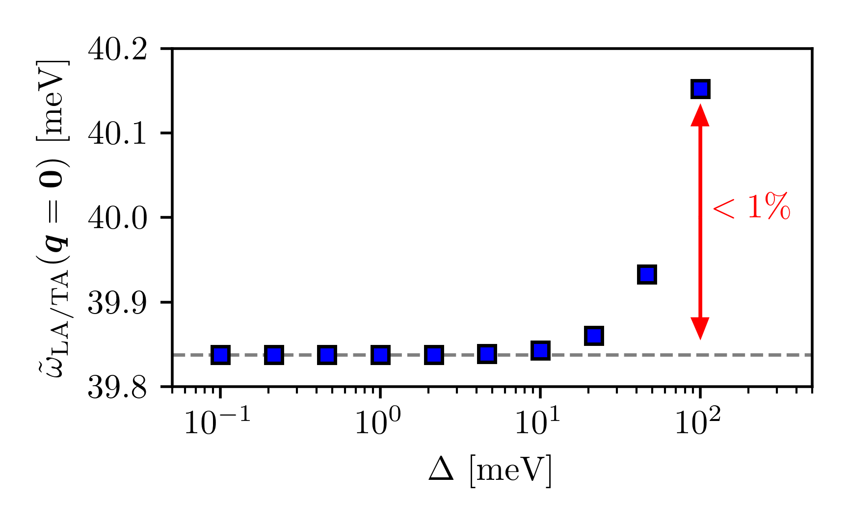
Figure 2: (Color online) Frequency of the degenerate acoustic branches at $\bm{q}=\bm{0}$. It is calculated after removing the geometric contribution to the dynamical matrix for different values of the regularizing Semenoff mass $\Delta$ and shows convergence for $\Delta\to 0$. Varying $\Delta$ over three orders of magnitude alters the phonon gap value by less than $1\%$. This result is reasonable, as the magnitude of the regularizer must be compared to the dominant electronic energy scale, which is the nearest-neighbor hopping amplitude $t^{(1)}\approx 3$ eV.

\begin{overpic}[width=108.405pt]{figures/sm_fig3a.png} \put(-4.0,147.0){\rm{(a)}} \end{overpic}	\begin{overpic}[width=108.405pt]{figures/sm_fig3b.png} \put(7.0,147.0){\rm{(b)}} \end{overpic}
\begin{overpic}[width=108.405pt]{figures/sm_fig3c.png} \put(-4.0,140.0){\rm{(c)}} \put(120.0,100.0){$\bm{K}$} \put(120.0,57.0){$\bm{K^{\prime}}$} \end{overpic}	\begin{overpic}[width=108.405pt]{figures/sm_fig3d.png} \put(7.0,140.0){\rm{(d)}} \put(120.0,100.0){$\bm{K}$} \put(120.0,57.0){$\bm{K^{\prime}}$} \end{overpic}

Figure 3: (Color online) Regularized QGT for gapped graphene. For better illustration, results in this figure have been calculated with a large gap of $\Delta=20~{\rm meV}$. (a) Trace of the Fubini-Study metric $g^{(\pm)}_{ij}(\bm{k})$— which is the same for both conduction and valence bands due to the quasi-exact particle-hole symmetry in the vicinity of the $\bm{K}$ point—plotted along the path in the FBZ shown as a red arrow in the inset. Cyan circles: numerical results obtained within the NN tight-binding model. Magenta squares: numerical results obtained within the NNNN model. Solid blue line: analytical results for massive Dirac fermions. (b) The only non-zero component of the conduction-band Berry curvature, ${\cal F}_{xy}^{(+)}(\bm{k})\equiv-2\operatorname{Im}{\cal Q}_{xy}^{(+)}(\bm{k})={\cal F}_{yx}^{(-)}(\bm{k})$, plotted along the same path as in panel (a). The valence-band curvature is identical apart from a sign. Legend is the same as in panel (a). (c)-(d) 2D color plots of $g^{(\pm)}_{ij}(\bm{k})$ and ${\cal F}_{xy}^{(+)}(\bm{k})$ calculated within the NNNN model as functions of $\bm{k}$. The insets provide a zoom-in view of the $\bm{K}$ point, where the singularity discussed in the text has been cured.

In order to obtain a complete description of electrons and phonons in graphene, as well as extract the relevant parameters of the hopping function within the Gaussian approximation, we have carried out ab initio density functional theory (DFT) and density-functional perturbation theory (DFPT) [9] calculations using Quantum ESPRESSO (QE) [10, 11].

The necessary pseudopotentials were taken from the standard solid-state pseudopotential (SSSP) accuracy library [12, 13]. The exchange-correlation potential was treated in the Generalized Gradient Approximation (GGA), as parametrized by the Perdew-Burke-Ernzerhof (PBE) formula [72], with the vdW-D2 correction proposed by Grimme [15]. For integrations over the FBZ, we employed a Methfessel-Paxton smearing function [16] of $10^{-2}~{\rm Ryd}$. A dense Monkhorst-Pack (MP) [17] ${\bm{k}}$-point grid with $96\times 96\times 1$ points is chosen to sample for self-consistent calculations of the charge density. The equilibrium lattice parameter of graphene is $a=2.467~{\rm\AA}$. We considered a simulation cell with approximately $22~{\rm\AA}$ of vacuum between periodic images along the $c$-direction. We also introduced a 2D Coulomb cutoff for a better description of phonons at small wavevectors [18].

The next-nearest-neighbor (NNN) Born-von Karman model for in-plane phonon dispersion has four force constants $\alpha,\beta,\gamma,\delta$ as free parameters. These parameters are optimized via least absolute deviations fitting to DFPT results.

The electronic dispersion in graphene is described by a next-next-nearest-neighbor (NNNN) tight-binding model [19], which depends on seven parameters: three hopping integrals $t^{(i)}$, three overlap integrals $s^{(i)}$ with $i=1,2,3$, and an on-site energy $\varepsilon_{p_{z}}$. The latter parameter can be set equal to zero due to gauge freedom. The remaining six physical parameters are determined via a least-squares procedure applied to the results of our DFT calculations. The results of this procedure are reported in Fig. 1. Fixing the six above-mentioned parameters allows us to reconstruct the Bloch Hamiltonian $h(\bm{k})$ on the entire FBZ, thus obtaining the Bloch eigenvectors $U_{n}(\bm{k})$ and the electron bands $E_{n}(\bm{k})$ with $\bm{k}\in\rm FBZ$. The reconstructed Hamiltonian is then regularized following the standard prescription [20]

$$h(\bm{k})\to h(\bm{k})+\begin{pmatrix}\Delta/2&0\\ 0&-\Delta/2\end{pmatrix}~,$$ (37)

fixing a gap $\Delta=1$ meV at the Dirac point. Numerical analysis has demonstrated that the gap size does not influence the key features $\tilde{\omega}_{\ell}(\bm{q})$ curves along the high-symmetry $\Gamma$KM$\Gamma$ contour, as shown for $\bm{q}=\bm{0}$ in Fig. 2. The regularized Fubini-Study metric and Berry curvature are shown in Fig. 3.

The hopping functions in graphene are modeled within the Gaussian approximation (Eq. (22) in the main text):

$$t^{p_{z}p_{z}}_{AB}(r)=t^{p_{z}p_{z}}_{AB}(0)\exp\left(\frac{1}{2}\gamma^{\vphantom{*}}_{AB}r^{2}\right)~,\qquad t^{p_{z}p_{z}}_{AA}(r)=t^{p_{z}p_{z}}_{AA}(0)\exp\left(\frac{1}{2}\gamma^{\vphantom{*}}_{AA}r^{2}\right)~.$$ (38)

Clearly, NN- and NNNN-type hopping integrals are parametrized by the first of the two equations above, while NNN-type hopping integrals are parametrized by the second one. The spatial dependence of the hopping integrals is determined as follows: after calculating the hopping integrals $t^{(1,2,3)}$ for a relaxed graphene lattice with lattice constant $a$, starting from the band structure as discussed above, the procedure is repeated by calculating electron bands on strained graphene lattices, i.e. graphene lattices whose lattice spacing $a^{*}$ is imposed to be $a^{*}\neq a$. This approach allows us to extract sufficient information about the spatial dependence of $t^{(1,2,3)}(r)$ to perform a Gaussian interpolation, as shown in Fig. 1. From this interpolation, the relevant parameters are estimated to be $\gamma_{AA}^{\vphantom{*}}=-1.37$ Å^-2 and $\gamma_{AB}^{\vphantom{*}}=-1.10$ Å^-2.

Summations over electron wavevectors $\bm{k}\in{\rm FBZ}$ appearing in Eqs. (14)-(15) have been carried out on a $N=420\times 420$ grid within the hexagonal FBZ. The evaluation of ${\cal D}_{\rm g}(\bm{q})$ at fixed $\bm{q}$ was repeated for each phonon wavevector $\bm{q}\in\Gamma{\rm KM}\Gamma$.

Appendix IX Calculation of the diagonal terms in ${\cal D}^{(2)}_{\rm g}(0)$ for massless Dirac fermions

We want to prove, with a fully analytical argument, the well-definiteness of our results when the derivative regularization parameter, i.e. the Semenoff mass $\Delta$, is equal to zero. Thus, we explicitly calculate the diagonal terms of the contribution ${\cal D}_{\rm g}(0)$ in Eq. (34) for the case of massless Dirac fermions, for which the energy bands are

$$\varepsilon_{\pm,\bm{k}}=\pm\varepsilon_{\bm{k}}=\pm\hbar v_{\rm F}k~,$$ (39)

and $v_{\rm F}=3a|t|/2\hbar$ is the Fermi velocity. We obtain

$$\begin{split}\bigl{[}{\cal D}^{\rm(2)}_{\rm g}(\bm{q}=\bm{0})\bigr{]}_{Ax}^{Ax}&=-\frac{1}{{M_{\rm C}}}\,\frac{2}{N}\sum_{\bm{k}}^{\text{FBZ}}\left\{\Bigl{[}\bigl{[}M^{\rm g}_{xx}(\bm{k})\bigr{]}_{A}^{B}+\bigl{[}M^{\rm E-g}_{xx}(\bm{k})\bigr{]}_{A}^{B}\Bigr{]}\bigl{[}P_{-}(\bm{k})\bigr{]}_{B}^{A}+\rm{H.c.}\right\}\\ &\simeq-\frac{2}{{M_{\rm C}}}\,\int_{D(\kappa)}\frac{{\rm d}^{2}k}{\pi\kappa^{2}}\,\gamma^{2}\frac{5\hbar^{4}v_{\rm F}^{4}}{\varepsilon_{\bm{k}}^{3}}\left(1-5\frac{\hbar^{2}v_{\rm F}^{2}}{\varepsilon_{\bm{k}}^{2}}k_{x}^{2}\right)k_{x}^{2}\\ &=-\frac{10\hbar v_{\rm F}\gamma^{2}}{M_{\rm C}\pi\kappa^{2}}\int_{0}^{\kappa}k\,\mathrm{d}k\int_{0}^{2\pi}\mathrm{d}\varphi\,\frac{1}{k^{3}}\left[1-5\cos^{2}\varphi\right]k^{2}\cos^{2}\varphi\\ &=\frac{55\hbar v_{\rm F}\gamma^{2}}{2M_{\rm C}\kappa}~,\end{split}$$ (40)

$$\begin{split}\bigl{[}{\cal D}^{\rm(2)}_{\rm g}(\bm{q}=\bm{0})\bigr{]}_{Ay}^{Ay}&=-\frac{1}{{M_{\rm C}}}\,\frac{2}{N}\sum_{\bm{k}}^{\text{FBZ}}\left\{\Bigl{[}\bigl{[}M^{\rm g}_{yy}(\bm{k})\bigr{]}_{A}^{B}+\bigl{[}M^{\rm E-g}_{yy}(\bm{k})\bigr{]}_{A}^{B}\Bigr{]}\bigl{[}P_{-}(\bm{k})\bigr{]}_{B}^{A}+\rm{H.c.}\right\}\\ &\simeq-\frac{2}{{M_{\rm C}}}\int_{D(\kappa)}\frac{{\rm d}^{2}k}{\pi\kappa^{2}}\,\gamma^{2}\frac{5\hbar^{4}v_{\rm F}^{4}}{\varepsilon_{\bm{k}}^{3}}\left(1-5\frac{\hbar^{2}v_{\rm F}^{2}}{\varepsilon_{\bm{k}}^{2}}k_{y}^{2}\right)(k_{x}+4k_{y})k_{x}\\ &=-\frac{10\hbar v_{\rm F}\gamma^{2}}{M_{\rm C}\pi\kappa^{2}}\int_{0}^{\kappa}k\,\mathrm{d}k\int_{0}^{2\pi}\mathrm{d}\varphi\,\frac{1}{k^{3}}\left[1-5\sin^{2}\varphi\right]k^{2}\cos^{2}\varphi\\ &=\frac{5\hbar v_{\rm F}\gamma^{2}}{2M_{\rm C}\kappa}~,\end{split}$$ (41)

where $\kappa$ is an integration cutoff around the $\bm{K}$ point. By direct calculation, we found that the integrals (40)-(41) are well-definite and finite for $\Delta=0$. The $\nu=\nu^{\prime}=B$ diagonal terms are identical due to the fact that exchanging sublattices only affects the imaginary part of the integrand, which is cancelled out by the Hermitian conjugate.

The ultraviolet cutoff $\kappa$ can be chosen as [21]

$$\kappa=2\eta\sqrt{\frac{\pi}{{\cal A}_{0}}}\sim\frac{1}{a}~,$$ (42)

where ${\cal A}_{0}=3\sqrt{3}a^{2}/2$ is the area of the unit cell of the honeycomb lattice, and $\eta\in[0,1]$ is a number which can be fine-tuned such that the result of the discrete sum appearing in the first lines of Eqs. (40)-(41) matches the value of the integral introduced in the second line.

References

- [1] G. Grosso and G. Pastori Parravicini, Solid State Physics, 2nd edition (Academic Press, Oxford, 2014).
- [2] M. P. Marder, Condensed Matter Physics, 2nd edition (John Wiley & Sons, Inc., New Jersey, 2010).
- [3] M. Tinkham, Introduction to Superconductivity, 2nd edition (Dover Publications, New York, 2004).
- [4] A. K. Geim and I. V. Grigorieva, Van der Waals heterostructures Nature 499, 419 (2013).
- [5] L. Wang, I. Meric, P. Y. Huang, Q. Gao, Y. Gao, H. Tran, T. Taniguchi, K. Watanabe, L. M. Campos, D. A. Muller, J. Guo, P. Kim, J. Hone, K.L. Shepard, and C. R. Dean, One-dimensional electrical contact to a two-dimensional material, Science 342, 614 (2013).
- [6] N. Mounet and N. Marzari, First-principles determination of the structural, vibrational and thermodynamic properties of diamond, graphite, and derivatives, Phys. Rev. B 71, 205214 (2005).
- [7] A. C. Ferrari, J. C. Meyer, V. Scardaci, C. Casiraghi, M. Lazzeri, F. Mauri, S. Piscanec, D. Jiang, K. S. Novoselov, S. Roth, and A. K. Geim, Raman spectrum of graphene and graphene layers, Phys. Rev. Lett. 97, 187401 (2006).
- [8] A. C. Ferrari, Raman spectroscopy of graphene and graphite: Disorder, electron–phonon coupling, doping and nonadiabatic effects, Solid State Commun. 143, 47 (2007).
- [9] D. L. Nika and A. A. Balandin, Two-dimensional phonon transport in graphene, J. Phys. Condens. Matter 24, 233203 (2012).
- [10] A. C. Ferrari and D. Basko, Raman spectroscopy as a versatile tool for studying the properties of graphene, Nature Nanotech. 8, 235 (2013).
- [11] A. Principi, M. Carrega, M. B. Lundeberg, A. Woessner, F. H. L. Koppens, G. Vignale, and M. Polini, Plasmon losses due to electron-phonon scattering: The case of graphene encapsulated in hexagonal boron nitride. Phys. Rev. B 90, 165408 (2014).
- [12] A. Woessner, M. B. Lundeberg, Y. Gao, A. Principi, P. Alonso-González, M. Carrega, K. Watanabe, T. Taniguchi, G. Vignale, M. Polini, J. Hone, R. Hillenbrand, and F. H. L. Koppens, Highly confined low-loss plasmons in graphene–boron nitride heterostructures, Nat. Mater. 14, 421 (2015).
- [13] M. B. Lundeberg, Y. Gao, R. Asgari, C. Tan, B. Van Duppen, M. Autore, P. Alonso-González, A. Woessner, K. Watanabe, T. Taniguchi, R. Hillenbrand, J. Hone, M. Polini, and F. H. L. Koppens, Tuning quantum nonlocal effects in graphene plasmonics, Science 357, 187 (2017).
- [14] G. X. Ni, A. S. McLeod, Z. Sun, L. Wang, L. Xiong, K. W. Post, S. S. Sunku, B.-Y. Jiang, J. Hone, C. R. Dean, M. M. Fogler, and D. N. Basov, Fundamental limits to graphene plasmonics, Nature 557, 530 (2018).
- [15] H. Leutwyler, Phonons as Goldstone bosons, Helv. Phys. Acta 70, 275 (1997).
- [16] S. Endlich, A. Nicolis, and J. Wang, Solid inflation, J. Cosmol. Astropart. Phys. 10, 011 (2013).
- [17] A. Nicolis, R. Penco, F. Piazza, and R. Rattazzi, Zoology of condensed matter: framids, ordinary stuff, extra-ordinary stuff, J. High Energ. Phys. 2015, 155 (2015).
- [18] A. Esposito, E. Geoffray, and T. Melia, Effective field theory for acoustic and pseudoacoustic phonons in solids, Phys. Rev. D 102, 105009 (2020).
- [19] F. Giustino, Electron-phonon interactions from first principles, Rev. Mod. Phys. 89, 015003 (2017).
- [20] M. Engel, M. Marsman, C. Franchini, and G. Kresse, Electron-phonon interactions using the projector augmented-wave method and Wannier functions, Phys. Rev. B 101, 184302 (2020).
- [21] J. Li, J. Li, J. Tang, Z. Tao, S. Xue, J. Liu, H. Peng, X.-Q. Chen, J. Guo, and X. Zhu, Direct observation of topological phonons in graphene, Phys. Rev. Lett. 131, 116602 (2023).
- [22] Y. Xu, M. G. Vergniory, D.-S. Ma, J. L. Mañes, Z.-D. Song, B. A. Bernevig, N. Regnault, and L. Elcoro, Catalog of topological phonon materials, Science 384, 638 (2024).
- [23] R. Resta, Manifestations of Berry’s phase in molecules and condensed matter, J. Phys. Condens. Matter 12, R107 (2000).
- [24] D. Vanderbilt, Berry Phases in Electronic Structure Theory (Cambridge University Press, Cambridge, 2018).
- [25] D. Xiao, M.-C. Chang, and Q. Niu, Berry phase effects on electronic properties, Rev. Mod. Phys. 82, 1959 (2010).
- [26] B. A. Bernevig and T. L. Hughes, Topological Insulators and Topological Superconductors (Princeton University Press, Princeton and Oxford, 2013).
- [27] P. Törmä, Essay: where can quantum geometry lead us?, Phys. Rev. Lett. 131, 240001 (2023).
- [28] J. Yu, B. A. Bernevig, R. Queiroz, E. Rossi, P. Törmä, and B.-J. Yang, Quantum Geometry in Quantum Materials, arXiv:2501.00098.
- [29] J. P. Provost and G. Vallee, Riemannian structure on manifolds of quantum states, Comm. Math. Phys. 76, 289 (1980).
- [30] D. N. Page, Geometrical description of Berry’s phase, Phys. Rev. A 36, 3479 (1987).
- [31] J. Anandan and Y. Aharonov, Geometry of quantum evolution, Phys. Rev. Lett. 65, 1697 (1990).
- [32] M. V. Berry, Quantal phase factors accompanying adiabatic changes, Proc. R. Soc. London, Ser. A 392, 45 (1984).
- [33] See Supplemental Material for additional information on the QGT in crystals, proof of the acoustic sum rules, calculation of electronic force constants within the BOA, explicit formulas for the dynamical matrix, discussion of the analogy between phonon theory and linear response theory, proof of the TRK sum rule for a 1D toy model, isolation of non-trivial geometric terms via the Gaussian approximation, details on the application of the theory to graphene, and explicit analytical calculation of some terms in for massless Dirac fermions.
- [34] R. Resta and S. Sorella, Electron localization in the insulating state, Phys. Rev. Lett. 82, 370 (1999).
- [35] I. Souza, T. Wilkens, and R. M. Martin, Polarization and localization in insulators: Generating function approach, Phys. Rev. B 62, 1666 (2000).
- [36] R. Resta, The insulating state of matter: A geometrical theory, Eur. Phys. J. B 79, 121 (2011).
- [37] M. F. Lapa and T. L. Hughes, Semiclassical wave packet dynamics in nonuniform electric fields, Phys. Rev. B 99, 121111 (2019).
- [38] S. Kwon and B.-J. Yang, Quantum geometric bound and ideal condition for Euler band topology, Phys. Rev. B 109, L161111 (2024).
- [39] Y. Onishi and L. Fu, Fundamental bound on topological gap, Phys. Rev. X 14, 011052 (2024).
- [40] I. Komissarov, T. Holder, and R. Queiroz, The quantum geometric origin of capacitance in insulators, Nat. Comm. 15, 4621 (2024).
- [41] N. Verma and R. Queiroz, Instantaneous response and quantum geometry of insulators, arXiv:2403.07052.
- [42] S. Peotta and P. Törmä, Superfluidity in topologically nontrivial flat bands, Nature Commun. 6, 8944 (2015).
- [43] J. S. Hofmann, E. Berg, and D. Chowdhury, Superconductivity, pseudogap, and phase separation in topological flat bands, Phys. Rev. B 102, 201112 (2020).
- [44] J. Herzog-Arbeitman, A. Chew, K.-E. Huhtinen, P. Törmä, and B. A. Bernevig, Many-Body superconductivity in topological flat bands, arXiv:2209.00007.
- [45] E. Rossi, Quantum metric and correlated states in two-dimensional systems, Curr. Opin. Solid State Mater. Sci. 25, 100952 (2021).
- [46] P. Törmä, S. Peotta, and B. A. Bernevig, Superconductivity, superfluidity and quantum geometry in twisted multilayer systems, Nat. Rev. Phys. 4, 528 (2022).
- [47] S. Peotta, K.-E. Huhtinen, and P. Törmä, Quantum geometry in superfluidity and superconductivity, arXiv:2308.08248.
- [48] J. S. Hofmann, E. Berg, and D. Chowdhury, Superconductivity, charge density wave, and supersolidity in flat bands with a tunable quantum metric, Phys. Rev. Lett. 130, 226001 (2023).
- [49] A. Kruchkov, Quantum transport anomalies in dispersionless quantum states, Phys. Rev. B 107, L241102 (2023).
- [50] J. Ahn, G.-Y. Guo, N. Nagaosa, and A. Vishwanath, Riemannian geometry of resonant optical responses, Nat. Phys. 18, 290 (2021).
- [51] C.-R. Yi, J. Yu, H. Yuan, R.-H. Jiao, Y.-M. Yang, X. Jiang, J.-Y. Zhang, S. Chen, and J.-W. Pan, Extracting the quantum geometric tensor of an optical Raman lattice by Bloch-state tomography, Phys. Rev. Res. 5, L032016 (2023).
- [52] M. Yu, P. Yang, M. Gong, Q. Cao, Q. Lu, H. Liu, S. Zhang, M. B. Plenio, F. Jelezko, T. Ozawa, N. Goldman, and J. Cai, Experimental measurement of the quantum geometric tensor using coupled qubits in diamond, Natl. Sci. Rev. 7, 254 (2019).
- [53] W. Zheng, J. Xu, Z. Ma, Y. Li, Y. Dong, Y. Zhang, X. Wang, G. Sun, P. Wu, J. Zhao, S. Li, D. Lan, X. Tan, and Y. Yu, Measuring quantum geometric tensor of non-Abelian system in superconducting circuits, Chin. Phys. Lett. 39, 100202 (2022).
- [54] A. Gianfrate, O. Bleu, L. Dominici, V. Ardizzone, M. De Giorgi, D. Ballarini, G. Lerario, K. W. West, L. N. Pfeiffer, D. D. Solnyshkov, D. Sanvitto, and G. Malpuech, Measurement of the quantum geometric tensor and of the anomalous Hall drift, Nature 578, 381 (2020).
- [55] R. K. Kumar, G. Li, R. Bertini, S. Chaudhary, K. Nowakowski, J. M. Park, S. Castilla, Z. Zhan, P. A. Pantaleón, H. Agarwal, S. Battle-Porro, E. Icking, M. Ceccanti, A. Reserbat-Plantey, G. Piccinini, J. Barrier, E. Khestanova, T. Taniguchi, K. Watanabe, C. Stampfer, G. Refael, F. Guinea, P. Jarillo-Herrero, J. C. W. Song, P. Stepanov, C. Lewandowski, and F. H. L. Koppens, Terahertz photocurrent probe of quantum geometry and interactions in magic-angle twisted bilayer graphene, arXiv:2406.16532.
- [56] J. Yu, C. J. Ciccarino, R. Bianco, I. Errea, P. Narang, and B. A. Bernevig, Non-trivial quantum geometry and the strength of electron–phonon coupling, Nature Phys. 20, 1262 (2024).
- [57] T. Holstein, Studies of polaron motion: Part I. The molecular-crystal model, Ann. Phys. 8, 325 (1959).
- [58] T. Holstein, Studies of polaron motion: Part II. The “small” polaron, Ann. Phys. 8, 343 (1959).
- [59] J. Sous, B. Kloss, D. M. Kennes, D. R. Reichman, and A. J. Millis, Phonon-induced disorder in dynamics of optically pumped metals from nonlinear electron-phonon coupling, Nat. Commun. 12, 5803 (2021).
- [60] G. F. Giuliani and G. Vignale, Quantum Theory of the Electron Liquid (Cambridge University Press, Cambridge, 2005).
- [61] X. Gonze and C. Lee, Dynamical matrices, Born effective charges, dielectric permittivity tensors, and interatomic force constants from density-functional perturbation theory, Phys. Rev. B 55, 10355 (1997).
- [62] M. A. H. Vozmediano, M. I. Katsnelson, and F. Guinea, Gauge fields in graphene, Phys. Rep. 496, 109 (2010).
- [63] J. J. Sakurai and J. Napolitano, Modern Quantum Mechanics, 2nd edition (Cambridge University Press, Cambridge, 2017).
- [64] G. M. Andolina, F. M. D. Pellegrino, V. Giovannetti, A. H. MacDonald, and M. Polini, Cavity quantum electrodynamics of strongly correlated electron systems: A no-go theorem for photon condensation, Phys. Rev. B 100, 121109 (2019).
- [65] Throughout this work we have taken the liberty to omit orbital and sublattice indices when referring to the projection matrix and the Bloch eigenvectors . These indices have instead been written down explicitly for the hopping matrix , the force-constant matrix , and the DM . Other quantities defined in the following, such as the Bloch Hamiltonian and its derivatives and , trivially inherit their matrix structure from the hopping matrix . Wherever the symbol appears in front of a matrix, e.g. , the product is intended to be element-wise, i.e. and . The same applies when .
- [66] L. Falkovsky, Phonon dispersion in graphene, J. Exp. Theor. Phys. 105, 397 (2007).
- [67] S. Baroni, S. de Gironcoli, A. Dal Corso, and P. Giannozzi, Phonons and related crystal properties from density-functional perturbation theory, Rev. Mod. Phys. 73, 515 (2001).
- [68] P. Giannozzi, S. Baroni, N. Bonini, M. Calandra, R. Car, C. Cavazzoni, D. Ceresoli, G. L. Chiarotti, M. Cococcioni, I. Dabo, A. Dal Corso, S. de Gironcoli, S. Fabris, G. Fratesi, R. Gebauer, U. Gerstmann, C. Gougoussis, A. Kokalj, M. Lazzeri, L. Martin-Samos, N. Marzari, F. Mauri, R. Mazzarello, S. Paolini, A. Pasquarello, L. Paulatto, C. Sbraccia, S. Scandolo, G. Sclauzero, A. P. Seitsonen, A. Smogunov, P. Umari, and R. M. Wentzcovitch, QUANTUM ESPRESSO: a modular and open-source software project for quantum simulations of materials, J. Phys. Condens. Matter 21, 395502 (2009).
- [69] P. Giannozzi, O. Andreussi, T. Brumme, O. Bunau, M. Buongiorno Nardelli, M. Calandra, R. Car, C. Cavazzoni, D. Ceresoli, M. Cococcioni, N. Colonna, I. Carnimeo, A. Dal Corso, S. de Gironcoli, P. Delugas, R. A. DiStasio, A. Ferretti, A. Floris, G. Fratesi, G. Fugallo, R. Gebauer, U. Gerstmann, F. Giustino, T. Gorni, J. Jia, M. Kawamura, H.-Y. Ko, A. Kokalj, E. Küçükbenli, M. Lazzeri, M. Marsili, N. Marzari, F. Mauri, N. L. Nguyen, H.-V. Nguyen, A. Otero-de-la-Roza, L. Paulatto, S. Poncé, D. Rocca, R. Sabatini, B. Santra, M. Schlipf, A. P. Seitsonen, A. Smogunov, I. Timrov, T. Thonhauser, P. Umari, N. Vast, X. Wu, and S. Baroni, Advanced capabilities for materials modelling with Quantum ESPRESSO, J. Phys. Condens. Matter 29, 465901 (2017).
- [70] G. Prandini, A. Marrazzo, I. E. Castelli, N. Mounet, and N. Marzari, Precision and efficiency in solid-state pseudopotential calculations, npj Comput. Mater. 4, 72 (2018).
- [71] A. Dal Corso, Pseudopotentials periodic table: From H to Pu, Comput. Mater. Sci. 95, 337 (2014).
- [72] J. P. Perdew, K. Burke, and M. Ernzerhof, Generalized gradient approximation made simple, Phys. Rev. Lett. 77, 3865 (1996).
- [73] S. Grimme, Semiempirical GGA-type density functional constructed with a long-range dispersion correction, J. Comput. Chem. 27, 1787 (2006).
- [74] M. Methfessel and A. T. Paxton, High-precision sampling for Brillouin-zone integration in metals, Phys. Rev. B 40, 3616 (1989).
- [75] H. J. Monkhorst and J. D. Pack, Special points for Brillouin-zone integrations, Phys. Rev. B 13, 5188 (1976).
- [76] T. Sohier, M. Calandra, and F. Mauri, Density functional perturbation theory for gated two-dimensional heterostructures: Theoretical developments and application to flexural phonons in graphene, Phys. Rev. B 96, 075448 (2017).
- [77] S. Reich, J. Maultzsch, C. Thomsen, and P. Ordejón, Tight-binding description of graphene, Phys. Rev. B 66, 035412 (2002).
- [78] M. I. Katsnelson, The Physics of Graphene, 2nd edition (Cambridge University Press, Cambridge, 2020).
- [79] G. Giovannetti, P. A. Khomyakov, G. Brocks, V. M. Karpan, J. van den Brink, and P. J. Kelly, Substrate-induced band gap in graphene on hexagonal boron nitride: Ab initio density functional calculations, Phys. Rev. B 76, 073103 (2007).
- [80] J. L. Mañes, Symmetry-based approach to electron-phonon interactions in graphene, Phys. Rev. B 76, 045430 (2007).
Supplemental Material for:

References

- [1] G. Grosso and G. Pastori Parravicini, Solid State Physics, 2nd edition (Academic Press, Oxford, 2014).
- [2] B. A. Bernevig and T. L. Hughes, Topological Insulators and Topological Superconductors (Princeton University Press, Princeton and Oxford, 2013).
- [3] R. Resta, The insulating state of matter: A geometrical theory, Eur. Phys. J. B 79, 121 (2011).
- [4] J. P. Provost and G. Vallee, Riemannian structure on manifolds of quantum states, Comm. Math. Phys. 76, 289 (1980).
- [5] J. Yu, C. J. Ciccarino, R. Bianco, I. Errea, P. Narang, and B. A. Bernevig, Non-trivial quantum geometry and the strength of electron–phonon coupling, Nature Phys. 20, 1262 (2024).
- [6] G. F. Giuliani and G. Vignale, Quantum Theory of the Electron Liquid (Cambridge University Press, Cambridge, 2005).
- [7] J. J. Sakurai and J. Napolitano, Modern Quantum Mechanics, 2nd edition (Cambridge University Press, Cambridge, 2017).
- [8] G. M. Andolina, F. M. D. Pellegrino, V. Giovannetti, A. H. MacDonald, and M. Polini, Cavity quantum electrodynamics of strongly correlated electron systems: A no-go theorem for photon condensation, Phys. Rev. B 100, 121109 (2019).
- [9] S. Baroni, S. de Gironcoli, A. Dal Corso, and P. Giannozzi, Phonons and related crystal properties from density-functional perturbation theory, Rev. Mod. Phys. 73, 515 (2001).
- [10] P. Giannozzi, S. Baroni, N. Bonini, M. Calandra, R. Car, C. Cavazzoni, D. Ceresoli, G. L. Chiarotti, M. Cococcioni, I. Dabo, A. Dal Corso, S. de Gironcoli, S. Fabris, G. Fratesi, R. Gebauer, U. Gerstmann, C. Gougoussis, A. Kokalj, M. Lazzeri, L. Martin-Samos, N. Marzari, F. Mauri, R. Mazzarello, S. Paolini, A. Pasquarello, L. Paulatto, C. Sbraccia, S. Scandolo, G. Sclauzero, A. P. Seitsonen, A. Smogunov, P. Umari, and R. M. Wentzcovitch, QUANTUM ESPRESSO: a modular and open-source software project for quantum simulations of materials, J. Phys. Condens. Matter 21, 395502 (2009).
- [11] P. Giannozzi, O. Andreussi, T. Brumme, O. Bunau, M. Buongiorno Nardelli, M. Calandra, R. Car, C. Cavazzoni, D. Ceresoli, M. Cococcioni, N. Colonna, I. Carnimeo, A. Dal Corso, S. de Gironcoli, P. Delugas, R. A. DiStasio, A. Ferretti, A. Floris, G. Fratesi, G. Fugallo, R. Gebauer, U. Gerstmann, F. Giustino, T. Gorni, J. Jia, M. Kawamura, H.-Y. Ko, A. Kokalj, E. Küçükbenli, M. Lazzeri, M. Marsili, N. Marzari, F. Mauri, N. L. Nguyen, H.-V. Nguyen, A. Otero-de-la-Roza, L. Paulatto, S. Poncé, D. Rocca, R. Sabatini, B. Santra, M. Schlipf, A. P. Seitsonen, A. Smogunov, I. Timrov, T. Thonhauser, P. Umari, N. Vast, X. Wu, and S. Baroni, Advanced capabilities for materials modelling with Quantum ESPRESSO, J. Phys. Condens. Matter 29, 465901 (2017).
- [12] G. Prandini, A. Marrazzo, I. E. Castelli, N. Mounet, and N. Marzari, Precision and efficiency in solid-state pseudopotential calculations, npj Comput. Mater. 4, 72 (2018).
- [13] A. Dal Corso, Pseudopotentials periodic table: From H to Pu, Comput. Mater. Sci. 95, 337 (2014).
- [14] J. P. Perdew, K. Burke, and M. Ernzerhof, Generalized gradient approximation made simple, Phys. Rev. Lett. 77, 3865 (1996).
- [15] S. Grimme, Semiempirical GGA-type density functional constructed with a long-range dispersion correction, J. Comput. Chem. 27, 1787 (2006).
- [16] M. Methfessel and A. T. Paxton, High-precision sampling for Brillouin-zone integration in metals, Phys. Rev. B 40, 3616 (1989).
- [17] H. J. Monkhorst and J. D. Pack, Special points for Brillouin-zone integrations, Phys. Rev. B 13, 5188 (1976).
- [18] T. Sohier, M. Calandra, and F. Mauri, Density functional perturbation theory for gated two-dimensional heterostructures: Theoretical developments and application to flexural phonons in graphene, Phys. Rev. B 96, 075448 (2017).
- [19] S. Reich, J. Maultzsch, C. Thomsen, and P. Ordejón, Tight-binding description of graphene, Phys. Rev. B 66, 035412 (2002).
- [20] M. I. Katsnelson, The Physics of Graphene, 2nd edition (Cambridge University Press, Cambridge, 2020).
- [21] M. Gibertini, A. Tomadin, M. Polini, A. Fasolino, and M. I. Katsnelson, Electron density distribution and screening in rippled graphene sheets, Phys. Rev. B 81, 125437, 2010.