“Short-length” Adversarial Training Helps LLMs
Defend “Long-length” Jailbreak Attacks:
Theoretical and Empirical Evidence

Abstract

Jailbreak attacks against large language models (LLMs) aim to induce harmful behaviors in LLMs through carefully crafted adversarial prompts. To mitigate attacks, one way is to perform adversarial training (AT)-based alignment, i.e., training LLMs on some of the most adversarial prompts to help them learn how to behave safely under attacks. During AT, the length of adversarial prompts plays a critical role in the robustness of aligned LLMs. This paper focuses on adversarial suffix jailbreak attacks and unveils that to defend against a jailbreak attack with an adversarial suffix of length $\Theta(M)$, it is enough to align LLMs on prompts with adversarial suffixes of length $\Theta(\sqrt{M})$. Theoretically, we analyze the adversarial in-context learning of linear transformers on linear regression tasks and prove a robust generalization bound for trained transformers. The bound depends on the term $\Theta(\sqrt{M_{\text{test}}}/M_{\text{train}})$, where $M_{\text{train}}$ and $M_{\text{test}}$ are the number of adversarially perturbed in-context samples during training and testing. Empirically, we conduct AT on popular open-source LLMs and evaluate their robustness against jailbreak attacks of different adversarial suffix lengths. Results confirm a positive correlation between the attack success rate and the ratio of the square root of the adversarial suffix during jailbreaking to the length during AT. Our findings show that it is practical to defend “long-length” jailbreak attacks via efficient “short-length” AT. The code is available at https://github.com/fshp971/adv-icl.

1 Introduction

Large language models (LLMs) (Brown et al., 2020; Touvron et al., 2023a; Liu et al., 2024a; Yang et al., 2024a) have been widely integrated into various real-world applications to assist human users, but their safety is found to be vulnerable toward jailbreak attacks (Wei et al., 2023). With carefully crafted adversarial prompts, one can “jailbreak” the safety mechanism of LLMs and induce arbitrary harmful behaviors (Zou et al., 2023; Chao et al., 2023; Liu et al., 2024b). To address this challenge, recent studies (Xhonneux et al., 2024; Mazeika et al., 2024; Yu et al., 2024; Casper et al., 2024) have proposed performing safety alignment through adversarial training (AT) (Madry et al., 2018) to enhance LLMs’ robustness against jailbreaking. A standard AT for LLMs would train them on harmful adversarial prompts synthesized by strong jailbreak attacks to learn to refuse these harmful instructions (Mazeika et al., 2024).

In such AT, the length of synthesized adversarial prompts used for model training is critical to the final jailbreak robustness of LLMs. Anil et al. (2024) and Xu et al. (2024) have shown that longer adversarial prompts enjoy stronger jailbreaking abilities. Thus, it is reasonable to deduce that performing AT with longer adversarial prompts can help LLMs achieve stronger robustness to defend against “long-length” jailbreak attacks. However, synthesizing long-length adversarial prompts in adversarial training is usually time-consuming since it requires solving discrete optimization problems in high-dimensional spaces. This may limit the application of AT in LLMs’ safety alignment and further raises the following research question:

How will the adversarial prompt length during AT affect trained LLMs’ robustness against jailbreaking with different prompt lengths?

This paper studies this research question by analyzing suffix jailbreak attacks, where each jailbreak prompt is constructed by concatenating a harmful instruction with a synthesized adversarial suffix. Our main finding is: To defend against a suffix jailbreak attack with suffix length of $\Theta(M)$, it is enough to adversarially train LLMs on adversarial prompts with suffix length of only $\Theta(\sqrt{M})$. In other words, we show that it is possible to defend long-length jailbreak attacks via efficient short-length AT.

Our finding is supported by theoretical and empirical evidence. Theoretically, we leverage the in-context learning theory (Von Oswald et al., 2023; Zhang et al., 2024) to investigate how linear transformers learn linear regression tasks from in-context task samples under AT. To better simulate suffix jailbreak attacks in real-world LLMs, our analysis introduces a new in-context adversarial attack. Concretely, for any in-context task sample, this attack will adversarially perturb the last several in-context training points to maximize the squared prediction error that linear transformers made on the in-context test point. Under our theoretical framework, we prove a robust generalization bound for adversarially trained linear transformers. This bound has a positive correlation with the term $\Theta(\sqrt{M_{\text{test}}}/M_{\text{train}})$, where $M_{\text{train}}$ and $M_{\text{test}}$ are the number of perturbed in-context points in training and testing in-context task samples, respectively.

Empirically, we conduct AT with the GCG attack (Zou et al., 2023), one of the most effective jailbreak attacks, under various adversarial suffix lengths on five popular real-world LLMs and evaluate their robustness against jailbreak attacks with different adversarial suffix lengths. We use the jailbreak attack success rate (ASR) to express the robust generalization error of trained LLMs and find that this ASR has a clear positive correlation with the ratio of the square root of test-time adversarial suffix length to the AT adversarial suffix length. Such a correlation empirically verifies our main finding. We also find that AT with an adversarial suffix (token) length of $20$ is already able to reduce the ASR of jailbreak attacks with an adversarial suffix (token) length of up to $120$ by at least $30\%$ in all experiments.

2 Related Works

Jailbreak attacks. Jailbreaking (Wei et al., 2023) can be seen as adversarial attacks (Szegedy et al., 2014; Goodfellow et al., 2015) toward LLMs, which aim to synthesize adversarial prompts to induce targeted harmful behaviors from LLMs. Many efforts have been made on token-level jailbreak attacks, i.e., searching adversarial prompts in the token space of LLMs, which can be achieved via gradient-based optimization (Shin et al., 2020; Guo et al., 2021; Zou et al., 2023; Liao and Sun, 2024; Schwinn et al., 2024), heuristic greedy search (Sadasivan et al., 2024; Hayase et al., 2024; Jin et al., 2024), or fine-tuning prompt generators from pre-trained LLMs (Paulus et al., 2024). Other attempts include word-level adversarial prompt searching (Liu et al., 2024b) or directly prompting LLMs to generate adversarial prompts (Chao et al., 2023; Liu et al., 2024c). Our work focuses on token-level jailbreaking since it make it easier for us to control the adversarial prompt length for our analysis.

More recent studies have found that increasing the length of adversarial prompts by adding more harmful demonstrations (Anil et al., 2024) or synthesizing longer adversarial suffixes (Xu et al., 2024) can make jailbreaking more effective. These works motivate us to investigate the problem of defending against “long-length” jailbreak attacks.

Adversarial training on LLMs. To defend against jailbreak attacks, a large body of studies focus on aligning LLMs to refuse responding jailbreak prompts (Ouyang et al., 2022; Rafailov et al., 2023; Qi et al., 2024a, b; Chen et al., 2024a). More recent works have started to adopt adversarial training (AT) (Madry et al., 2018) to align LLMs. Mazeika et al. (2024) trained LLMs on (discrete) adversarial prompts synthesized by GCG attack (Zou et al., 2023), in which they cached the intermediate synthesized results to reduce the heavy cost of searching adversarial prompts from scratch. Meanwhile, various studies (Xhonneux et al., 2024; Casper et al., 2024; Sheshadri et al., 2024; Yu et al., 2024) conduct AT with adversarial examples found in the continuous embedding space rather than the discrete text space since searching in the continuous embedding space is more computationally efficient. Nevertheless, as a preliminary study of the length of adversarial prompts during AT, our work only analyzes AT with discrete adversarial prompts.

In-context learning theory (ICL). Transformer-based large models like LLMs are strong in performing ICL: Given a series of inputs (also known as “prompt”) specified by a certain task, LLMs can make predictions well for this certain task without adjusting model parameters. Current theories in understanding ICL can be roughly divided into two categories. The first category aims to understand ICL via constructing explicit multi-layer transformers to simulate the optimization process of learning function classes (Garg et al., 2022; Von Oswald et al., 2023; Ahn et al., 2023; Chen et al., 2024b; Mahankali et al., 2024; Wang et al., 2024a). The second category focuses on directly analyzing the training (Zhang et al., 2024; Yang et al., 2024b; Huang et al., 2023; Wu et al., 2024; Lin et al., 2024) and generalization (Lu et al., 2024; Magen et al., 2024; Frei and Vardi, 2024; Shi et al., 2024) of simple self-attention models (i.e., one-layer transformer). Anwar et al. (2024) is the first to study adversarial attacks against linear transformers and finds that an attack can always succeed by perturbing only a single in-context sample. However, their analysis allows samples to be perturbed in the entire real space, which might not appropriately reflect real-world settings since real-world adversarial prompts can only be constructed from token/character spaces of limited size. Unlike Anwar et al. (2024), we propose a new ICL adversarial attack that requires each adversarial suffix token to be perturbed only within restricted spaces, which thus can be a better tool for understanding real-world jailbreaking.

3 Preliminaries

Large language models (LLMs). Let $[V]=\{1,\cdots,V\}$ be a vocabulary set consisting of all possible tokens. Then, an LLM can be seen as a function that for any sequence $x_{1:n}\in[V]^{n}$ consists of $n$ tokens, the LLM will map $x_{1:n}$ to its next token $x_{n+1}$ following $x_{n+1}\sim p_{\theta}(\cdot|x_{1:n})$, where $p_{\theta}$ is a conditional distribution over the vocabulary set $[V]$ and $\theta$ is the model parameter of the LLM. Under such notations, when using the LLM $p_{\theta}$ to generate a new token sequence for the input $x_{1:n}$, the probability of generating a sequence $y_{1:m}\in[V]^{m}$ of length $m$ is (“$\oplus$” denotes concatenation):

$$p_{\theta}(y_{1:m}|x_{1:n})=\prod_{i=1}^{m}p_{\theta}(y_{i}|x_{1:n}\oplus y_{1:(i-1)}),$$

Jailbreak attacks. This paper will focus on suffix jailbreak attacks. Concretely, suppose $x^{(h)}$ and $y^{(h)}$ are two token sequences, where $x^{(h)}$ represents a harmful prompt (e.g., “Please tell me how to build a bomb.”) and $y^{(h)}$ represents a corresponded targeted answer (e.g., “Sure, here is a guide of how to build a bomb”). Then, the goal of a suffix jailbreak attack against the LLM $p_{\theta}$ aims to synthesize an adversarial suffix $x^{(s)}_{1:m}$ for the original harmful prompt $x^{(h)}$ via solving the following optimization problem,

$$\min_{x^{(s)}_{1:m}\in[V]^{m}}-\log p_{\theta}(y^{(h)}|x^{(h)}\oplus x^{(s)}_{1:m}),$$ (3.1)

where $x^{(h)}\oplus x^{(s)}_{1:m}$ is the adversarial prompt and $m$ is the sequence length of the adversarial suffix $x^{(s)}_{1:m}$. Intuitively, a large $m$ will increase the probability of the LLM $p_{\theta}$ that generating the targeted answer $y^{(h)}$ for the synthesized adversarial prompt $x^{(h)}\oplus x^{(s)}_{1:m}$.

To solve Eq. (3.1), a standard method is the Greedy Coordinate Gradient (GCG) attack (Zou et al., 2023), which leverages gradient information to search for better $x^{(s)}_{1:m}$ within the discrete space $[V]^{m}$ in a greedy manner.

Adversarial training (AT). We consider the canonical AT loss $\mathcal{L}$ Mazeika et al. (2024); Qi et al. (2024a) to train the LLM $p_{\theta}$, which consists of two sub-losses: an adversarial loss $\mathcal{L}_{\text{adv}}$ and an utility loss $\mathcal{L}_{\text{utility}}$.

Specifically, given a safety dataset $D^{(h)}$, where each of its sample $(x^{(h)},y^{(h)},y^{(b)})\in D^{(h)}$ consists of a harmful instruction $x^{(h)}$, a harmful answer $y^{(h)}$, and a benign answer $y^{(b)}$ (e.g., “As a responsible AI, I can’t tell you how to…”). The adversarial loss $\mathcal{L}_{\text{adv}}$ is defined as follows,

$$\mathcal{L}_{\text{adv}}(\theta,M,D^{(h)}):=\mathop{\mathbb{E}}_{(x^{(h)},y^{(h)},y^{(b)})\in D^{(h)}}[-\log p_{\theta}(y^{(b)}|x^{(h)}\oplus x_{1:m}^{(s)})],$$ (3.2)

where $x^{(s)}_{1:m}$ is the adversarial suffix obtained from Eq. (3.1) and $m$ is the adversarial suffix length. Note that the probability terms in Eqs. (3.1) and (3.2) look similar to each other. The difference is that the term in Eq. (3.1) denotes the probability that $p_{\theta}$ generates the harmful answer $y^{(h)}$ for the adversarial prompt, while that in Eq. (3.2) denotes the probability of generating the benign answer $y^{(b)}$.

Besides, let $D^{(u)}$ be a utility dataset where each of its sample $(x^{(u)},y^{(u)})\in D^{(u)}$ consists of a pair of normal instruction and answer. Then, the utility loss $\mathcal{L}_{\text{utility}}$ is given by

$$\mathcal{L}_{\text{utility}}(\theta,D^{(u)}):=\mathop{\mathbb{E}}_{(x^{(u)},y^{(u)})\in D^{(u)}}[-\log p_{\theta}(y^{(u)}|x^{(u)})].$$

Thus, the overall AT optimization problem for improving the jailbreak robustness of the LLM $p_{\theta}$ is given as follows,

$$\min_{\theta}\{\alpha\mathcal{L}_{\text{adv}}(\theta,M,D^{(h)})+(1-\alpha)\mathcal{L}_{\text{utility}}(\theta,D^{(u)})\},$$ (3.3)

where $\alpha\in[0,1]$ is a factor that balances between the adversarial and utility sub-losses. The idea behind such a loss design is that: (1) help LLM learn to respond harmlessly even when strong jailbreak prompts present (achieved via $\mathcal{L}_{\text{adv}}$), (2) retain the utility of LLM gained from pre-training (achieved via $\mathcal{L}_{\text{utility}}$). Intuitively, a larger adversarial suffix length $m$ during AT will help the LLM gain robustness against jailbreak attacks with longer adversarial suffixes.

4 Theoretical Evidence

This section establishes the theoretical foundation of how “short-length” AT can defend against “long-length” jailbreaking. Our analysis is based on the in-context learning (ICL) theory (Zhang et al., 2024; Shi et al., 2024; Anwar et al., 2024), and we will bridge the ICL theory and the LLM AT problem defined in Eq. (3.3) later. Here we first introduce the necessary notations to describe the problem. To avoid confusion, we note that all notations in this section will only be used within this section and have no relevance to those in other sections (e.g., Section 3).

In-context learning (ICL). In the ICL theory, a prompt with length $N$ related to a specific task indexed by $\tau$ is defined as $(x_{\tau,1},y_{\tau,1},\cdots,x_{\tau,N},y_{\tau,N},x_{\tau,q})$, where $x_{\tau,i}\in\mathbb{R}^{d}$ is the $i$-th in-context training sample (demonstration), $y_{\tau,i}\in\mathbb{R}$ is the label for the $i$-th training sample, and $x_{\tau,q}\in\mathbb{R}^{d}$ is the in-context query sample. Then, the embedding matrix $E_{\tau}$ for this task-related prompt is defined as follows,

$$E_{\tau}:=\begin{pmatrix}x_{\tau,1}&\cdots&x_{\tau,N}&x_{\tau,q}\\ y_{\tau,1}&\cdots&y_{\tau,N}&0\\ \end{pmatrix}\in\mathbb{R}^{(d+1)\times(N+1)}.$$ (4.1)

Given a prompt embedding matrix $E_{\tau}$ of task $\tau$, the goal of an ICL model is to make a prediction based on $E_{\tau}$ for the query sample $x_{\tau,q}$. Such an ICL model design aims to model the ability of real-world LLMs in making decisions based on prompting without updating model parameters.

Linear self-attention (LSA) models. LSA models are a kind of linear transformer that has been widely adopted in existing theoretical ICL studies. Ahn et al. (2024) empirically show that LSA models share similar properties with non-linear ones and thus are useful for understanding transformers. We follow Zhang et al. (2024) to study the following single-layer LSA model,

$$f_{\text{LSA},\theta}(E_{\tau}):=\left[E_{\tau}+W^{V}E_{\tau}\cdot\frac{E_{\tau}^{\top}W^{KQ}E_{\tau}}{N}\right]\in\mathbb{R}^{(d+1)\times(N+1)}$$

where $\theta:=(W^{V},W^{KQ})$ is the model parameter, $W^{V}\in\mathbb{R}^{(d+1)\times(d+1)}$ is the value weight matrix, $W^{KQ}\in\mathbb{R}^{(d+1)\times(d+1)}$ is a matrix merged from the key and query weight matrices of attention models, $E_{\tau}\in\mathbb{R}^{(d+1)\times(N+1)}$ is the prompt embedding matrix, and $N$ is the prompt length. The model prediction $\hat{y}_{q,\theta}$ for the query sample $x_{\tau,q}$ is given by the right-bottom entry of the output matrix of the LSA model, i.e., $\hat{y}_{q,\theta}(E_{\tau}):=f_{\text{LSA},\theta}(E_{\tau})_{(d+1),(N+1)}$.

We further follow Zhang et al. (2024) to denote that

$$W^{V}=\begin{pmatrix}W^{V}_{11}&w^{V}_{12}\\ (w^{V}_{21})^{\top}&w^{V}_{22}\end{pmatrix}\in\mathbb{R}^{(d+1)\times(d+1)},\ \ W^{KQ}=\begin{pmatrix}W^{KQ}_{11}&w^{KQ}_{12}\\ (w^{KQ}_{21})^{\top}&w^{KQ}_{22}\end{pmatrix}\in\mathbb{R}^{(d+1)\times(d+1)},$$

where $W^{V}_{11},W^{KQ}_{11}\in\mathbb{R}^{d\times d}$, $w^{V}_{12},w^{V}_{21},w^{KQ}_{12},w^{KQ}_{21}\in\mathbb{R}^{d\times 1}$ and $w^{V}_{22},W^{KQ}_{22}\in\mathbb{R}$. Under this setting, the model prediction $\hat{y}_{q,\theta}$ can be further simplified as follows,

$$\hat{y}_{q,\theta}(E_{\tau}):=f_{\text{LSA},\theta}(E_{\tau})_{(d+1)\times(N+1)}=\begin{pmatrix}(w^{V}_{21})^{\top}&w^{V}_{22}\end{pmatrix}\cdot\frac{E_{\tau}E_{\tau}^{\top}}{N}\cdot\begin{pmatrix}W^{KQ}_{11}\\ (w^{KQ}_{21})^{\top}\end{pmatrix}\cdot x_{\tau,q}.$$ (4.2)

Other notations. We denote $[n]:=\{1,\cdots,n\}$ for any $n\in\mathbb{N}^{+}$. For any matrix $A\in\mathbb{R}^{n\times m}$, we denotes $\|A\|_{2,\infty}:=\max_{1\leq i\leq m}\|A_{i,:}\|_{2}$, $\|A\|_{2}$ be the operator norm, and $\|A\|_{F}$ be the Frobenius norm. $\mathrm{Tr}(A):=\sum_{i=1}^{n}A_{i,i}$ is the trace function for any matrix $A\in\mathbb{R}^{n\times n}$. Finally, we use standard big O notations $\mathcal{O}(\cdot)$ and $\Theta(\cdot)$.

4.1 Problem Definition for Adversarial ICL

We now formalize the AT problem in ICL with the previously introduced notations. Concretely, we focus on the linear regression task and introduce a novel in-context “suffix” adversarial attack, where in-context adversarial points are appended to the end of in-context prompts, to analyze the robustness of LSA models.

Data distribution and statistical model. For any task indexed by $\tau$, we assume that there is a task weight $w_{\tau}\in\mathbb{R}^{d}$ drawn from $w_{\tau}\sim\mathcal{N}(0,I_{d})$. Besides, for any in-context training point $x_{\tau,i}\ (1\leq i\leq N)$ and the query point $x_{\tau,q}$ (see Eq. (4.1)), we assume that they are drawn from $x_{\tau,i},x_{\tau,q}\sim\mathcal{N}(0,\Lambda)$, where $\Lambda\in\mathbb{R}^{d\times d}$ is a positive-definite covariance matrix. Moreover, the ground-truth labels of training points $x_{\tau,i}$ and the query point $x_{\tau,q}$ are given by $y_{\tau,i}=w_{\tau}^{\top}x_{\tau,i}$ and $y_{\tau,q}=w_{\tau}^{\top}x_{\tau,q}$.

ICL (suffix) adversarial attack. Our novel adversarial attack against ICL models is launched via concatenating (clean) prompt embedding matrices with adversarial embedding suffixes. Specifically, for a prompt embedding matrix $E_{\tau}$ of length $N$ (see Eq. (4.1)), we will form its corresponding adversarial prompt embedding matrix $E^{\text{adv}}_{\tau,M}\in\mathbb{R}^{(d+1)\times(N+M+1)}$ by concatenating $E_{\tau}$ with an adversarial suffix of length $M$ as follows,

$$E^{\text{adv}}_{\tau,M} :=\begin{pmatrix}\underbrace{\begin{pmatrix}X_{\tau}\\ Y_{\tau}\end{pmatrix}}_{\shortstack{\tiny Training Data \\ \tiny of Length $N$}}&\underbrace{\begin{pmatrix}X^{\text{sfx}}_{\tau}+\Delta_{\tau}\\ Y^{\text{sfx}}_{\tau}\end{pmatrix}}_{\shortstack{\tiny Adversarial Suffix \\ \tiny of Length $M$}}&\underbrace{\begin{pmatrix}x_{\tau,q}\\ 0\end{pmatrix}}_{\shortstack{\tiny Query Sample \\ \tiny From $E_{\tau}$}}\end{pmatrix},$$ (4.3)

where

$$\left\{\begin{aligned} X_{\tau}&:=\begin{pmatrix}x_{\tau,1}&\cdots&x_{\tau,N}\end{pmatrix}\in\mathbb{R}^{d\times N}\\ Y_{\tau}&:=\begin{pmatrix}y_{\tau,1}&\cdots&y_{\tau,N}\end{pmatrix}\in\mathbb{R}^{1\times N}\end{aligned}\right.$$

denote the $N$ original training samples and labels, and

$$\left\{\begin{aligned} X^{\text{sfx}}_{\tau}&:=\begin{pmatrix}x^{\text{sfx}}_{\tau,1}&\cdots&x^{\text{sfx}}_{\tau,M}\end{pmatrix}\in\mathbb{R}^{d\times M}\\ Y^{\text{sfx}}_{\tau}&:=\begin{pmatrix}y^{\text{sfx}}_{\tau,1}&\cdots&y^{\text{sfx}}_{\tau,M}\end{pmatrix}\in\mathbb{R}^{1\times M}\\ \Delta^{\text{sfx}}_{\tau}&:=\begin{pmatrix}\delta_{\tau,1}&\cdots&\delta_{\tau,M}\end{pmatrix}\in\mathbb{R}^{d\times M}\end{aligned}\right.$$

denotes the new $M$ clean suffix samples, clean suffix labels, and adversarial perturbations. The clean suffix samples $X^{\text{sfx}}_{\tau}$ and labels $Y^{\text{sfx}}_{\tau}$ here follow the same distribution as those in-context data in the embedding $E_{\tau}$, i.e., $x^{\text{sfx}}_{\tau,i}\sim\mathcal{N}(0,\Lambda)$ and $y^{\text{sfx}}_{\tau,i}=w_{\tau}^{\top}x^{\text{sfx}}_{\tau,i}$ hold for every $i\in[M]$. For the adversarial perturbation matrix $\Delta_{\tau}$, we require each perturbation $\delta_{\tau,i}$ is restricted within a ball-sphere as $\|\delta_{\tau,i}\|_{2}\leq\epsilon$, where $\epsilon>0$ is the perturbation radius. This aims to simulate that in jailbreak attacks, and each adversarial token is searched within a token vocabulary set of limited size.

The goal of the ICL adversarial attack is to add an optimal suffix adversarial perturbation matrix $\Delta_{\tau}$ to maximize the difference between the model prediction $\hat{y}_{q}(E^{\text{adv}}_{\tau})$ based on the adversarial prompt embedding matrix $E^{\text{adv}}_{\tau}$ and the ground-truth query label $y_{\tau,q}$. We adopt the squared loss to measure such a prediction difference, which thus leads to the robust generalization error for the model $f^{\text{LSA}}_{\theta}$ as follows,

$$\mathcal{R}^{\text{adv}}(\theta,M)=\mathop{\mathbb{E}}_{\tau}\max_{\|\Delta_{\tau}^{\top}\|_{2,\infty}\leq\epsilon}\frac{1}{2}|\hat{y}_{q,\theta}(E^{\text{adv}}_{\tau,M})-y_{\tau,q}|^{2},$$ (4.4)

where $M$ is the length of the adversarial suffix and the expectation $\mathop{\mathbb{E}}_{\tau}[\cdot]$ is calculated over the randomness of $w_{\tau}$, $X_{\tau}$, $X^{\text{sfx}}_{\tau}$, and $x_{\tau,q}$. Since this paper aims to understand how the adversarial prompt length in AT would affect the robustness of LLM, Eq. (4.4) will also only focus on how the adversarial suffix length $M$ in ICL adversarial attacks would affect the robust generalization error $\mathcal{R}^{\text{adv}}(\theta,M)$.

Adversarial in-context learning. Following previous studies on minimax AT (Madry et al., 2018; Javanmard et al., 2020; Ribeiro et al., 2023; Fu and Wang, 2024; Wang et al., 2024b), here we also adopt a minimax AT loss to train the LSA model. Concretely, we first use the aforementioned ICL adversarial attack to synthesize adversarial prompts and then update the LSA model based on these adversarial prompts to help the model gain robustness against adversarial prompts. We further assume that the adversarial suffix length is fixed during AT, which thus leads to the following AT optimization problem formalization,

$$\min_{\theta}\mathcal{L}^{\text{adv}}(\theta):=\min_{\theta}\mathcal{R}^{\text{adv}}(\theta,M_{\text{train}})=\min_{\theta}\left\{\mathop{\mathbb{E}}_{\tau}\max_{\|\Delta_{\tau}^{\top}\|_{2,\infty}\leq\epsilon}\frac{1}{2}|\hat{y}_{q,\theta}(E^{\text{adv}}_{\tau,M_{\text{train}}})-y_{\tau,q}|^{2}\right\},$$ (4.5)

where $\mathcal{L}^{\text{adv}}(\theta):=\mathcal{R}^{\text{adv}}(\theta,M_{\text{train}})$ is the AT loss in ICL and $M_{\text{train}}\in\mathbb{N}^{+}$ is the fixed adversarial suffix length during AT. We will perform AT with continuous gradient flow, and further following Zhang et al. (2024) to make the following assumption on the LSA model parameter initialization.

Assumption 1 (c.f. Assumption 3.3 in Zhang et al. (2024)).

Let $\sigma>0$ be a parameter and $\Theta\in\mathbb{R}^{d\times d}$ be any matrix satisfying $\|\Theta\Theta^{\top}\|_{F}=1$ and $\Theta\Lambda\neq 0_{d\times d}$. We assume that

$$W^{V}(0)=\left(\begin{matrix}0_{d\times d}&0_{d\times 1}\\ 0_{1\times d}&\sigma\end{matrix}\right),\ \ W^{KQ}(0)=\left(\begin{matrix}\sigma\Theta\Theta^{\top}&0_{d\times 1}\\ 0_{1\times d}&0\end{matrix}\right).$$

Recall in Eq. (4.2), $w^{V}_{12}$, $w^{KQ}_{12}$, and $w^{KQ}_{22}$ do not contribute to the model prediction function $\hat{y}_{q,\theta}(\cdot)$. Thus, Assumption 1 directly sets them to be zero at initialization. To ensure symmetric initialization, Assumption 1 further sets $w^{V}_{21}(0)$ and $w^{KQ}_{21}(0)$ to zero. In the next section, we will see how Assumption 1 helps simplify the analysis of ICL AT.

Bridging ICL AT and LLM AT. Finally, we explain the similarities between AT on ICL models and LLMs to motivate why ICL AT (i.e., Eq. (4.5)) can be a good artifact to theoretically understand LLM AT (i.e., Eq. (3.3)).

We first compare the ICL suffix adversarial attack in Eq. (4.4) with the LLM suffix jailbreak attack in Eq. (3.1). We find that their attack goals are similar since both attacks aim to make targeted models behave wrongly via manipulating suffixes of input prompts. The only difference is that jailbreak attacks aim to induce LLMs to generate specified harmful content while our ICL attack aims to maximize linear regression prediction errors made by ICL models. Besides, unlike Anwar et al. (2024), which performs ICL attacks by perturbing a single in-context sample in the entire real space, our attack allows perturbing multiple in-context samples but only within restricted spaces, thus better simulating how LLM jailbreak attacks allow adversarial token suffixes to be searched only in the limited token vocabulary set.

We then compare the ICL AT problem in Eq. (4.5) with the LLM AT problem in Eq. (3.3). One can find that the motivations behind the two AT problems are the same, which is to enhance models’ robustness by training them on adversarial prompts. However, we notice that the LLM AT problem introduces an additional utility loss to maintain the performance of LLMs on benign data. This is because in LLM jailbreak attacks, adversarial prompts would be crafted only from harmful prompts but not benign ones. We argue that this discrepancy has little impact on our theoretical analysis, as both our theory and experiments focus on studying how adversarially trained models can defend against adversarial prompts rather than their performance on benign data.

4.2 Training Dynamics of Adversarial ICL

We now start to analyze the training dynamics of the minimax ICL AT problem formalized in Eq. (4.5).

The main technical challenge is that to solve the inner maximization problem in Eq. (4.5), one needs to analyze the optimization of the adversarial perturbation matrix $\Delta_{\tau}$. However, the matrix $\Delta_{\tau}$ along with the clean data embedding $E_{\tau}$ and the clean adversarial suffix $(X^{\text{sfx}}_{\tau},Y^{\text{sfx}}_{\tau})$ are entangled together within the adversarial embedding matrix $E^{\text{adv}}_{\tau,M_{\text{train}}}$, which makes it very difficult to solve the inner maximization problem and further analyze the ICL AT dynamics.

To tackle such a challenge, we propose to instead study the dynamics of a closed-form upper bound of the original AT loss $\mathcal{L}^{\text{adv}}(\theta)$. Formally, we will analyze the following surrogate AT problem for the LSA model $f_{\text{LSA},\theta}$:

$$\min_{\theta}\tilde{\mathcal{L}}^{\text{adv}}(\theta):=\min_{\theta}\Bigl{\{}\sum_{i=1}^{4}\ell_{i}(\theta)\Bigr{\}},$$ (4.6)

where $\tilde{\mathcal{L}}^{\text{adv}}(\theta):=\sum_{i=1}^{4}\ell_{i}(\theta)$ is the surrogate AT loss, and

$$E^{\text{clean}}_{\tau,M_{\text{train}}}=\begin{pmatrix}X_{\tau}&X^{\text{sfx}}_{\tau}&x_{\tau,q}\\ Y_{\tau}&Y^{\text{sfx}}_{\tau}&0\end{pmatrix},$$

$$\ell_{1}(\theta)=2\mathop{\mathbb{E}}_{\tau}\Bigl{[}((w^{V}_{21})^{\top}\ \ w^{V}_{22})\frac{E^{\text{clean}}_{\tau,M_{\text{train}}}E^{\text{clean}\top}_{\tau,M_{\text{train}}}}{N+M_{\text{train}}}\begin{pmatrix}W^{KQ}_{11}\\ (w^{KQ}_{21})^{\top}\end{pmatrix}x_{\tau,q}-y_{\tau,q}\Bigr{]}^{2},$$

$$\ell_{2}(\theta)=\frac{2\epsilon^{4}M_{\text{train}}^{2}}{(N+M_{\text{train}})^{2}}\|w^{V}_{21}\|_{2}^{2}\mathop{\mathbb{E}}_{\tau}\Bigl{[}\|W^{KQ}_{11}x_{\tau,q}\|_{2}^{2}\Bigr{]},$$

$$\ell_{3}(\theta)=\frac{2\epsilon^{2}M_{\text{train}}}{(N+M_{\text{train}})^{2}}\mathop{\mathbb{E}}_{\tau}\Bigl{[}\|W^{KQ}_{11}x_{\tau,q}\|_{2}^{2}\cdot\|((w^{V}_{21})^{\top}\ \ w^{V}_{22})\begin{pmatrix}X^{\text{sfx}}_{\tau}\\ Y^{\text{sfx}}_{\tau}\end{pmatrix}\|_{2}^{2}\Bigr{]},$$

$$\ell_{4}(\theta)=\frac{2\epsilon^{2}M_{\text{train}}}{(N+M_{\text{train}})^{2}}\|w^{V}_{21}\|_{2}^{2}\cdot\mathop{\mathbb{E}}_{\tau}\Bigl{[}\|\begin{pmatrix}X^{\text{sfx}}_{\tau}\\ Y^{\text{sfx}}_{\tau}\end{pmatrix}^{\top}\begin{pmatrix}W^{KQ}_{11}\\ (w^{KQ}_{21})^{\top}\end{pmatrix}x_{\tau,q}\|_{2}^{2}\Bigr{]}.$$

In the surrogate AT problem defined as Eq. (4.6), the surrogate AT loss function $\tilde{\mathcal{L}}^{\text{adv}}(\theta)$ is the closed-form upper bound for the original AT loss function $\mathcal{L}^{\text{adv}}(\theta)$ in Eq. (4.5). This is illustrated in the following proposition:

Proposition 1.

For the AT loss function $\mathcal{L}^{\text{\rm adv}}(\theta)$ defined in Eq. (4.5) and the surrogate AT loss function $\tilde{\mathcal{L}}^{\text{\rm adv}}(\theta)$ defined in Eq. (4.6), for any model parameter $\theta:=(W^{V},W^{KQ})$ of the LSA model $f_{\text{\rm LSA},\theta}$, we uniformly have that

$$\mathcal{L}^{\text{\rm adv}}(\theta)\leq\tilde{\mathcal{L}}^{\text{\rm adv}}(\theta).$$

The proof of Proposition 1 is presented in Appendix A.2. This result indicates that when we are training the LSA model via solving the surrogate AT problem Eq. (4.6), we are also reducing the model training loss in the original AT problem Eq. (4.5). Thus, solving the surrogate AT problem will also intuitively improve the robustness of the model.

Based on our previous analysis, we now turn to study the training dynamics of surrogate AT defined in Eq. (4.6). To better describe our results, we define two functions $\Gamma(\cdot):\mathbb{N}\rightarrow\mathbb{R}^{d\times d}$ and $\psi(\cdot):\mathbb{N}\rightarrow\mathbb{R}$, both of which depend on the adversarial suffix length $M$, as follows,

$$\Gamma(M) :=\frac{N+M+1}{N+M}\Lambda+\frac{\mathrm{Tr}(\Lambda)}{N+M}I_{d}\in\mathbb{R}^{d\times d},$$ (4.7)

$$\psi(M) :=\frac{M^{2}\mathrm{Tr}(\Lambda)}{(N+M)^{2}}\in\mathbb{R},$$ (4.8)

where $N$ is the prompt length of the original embedding matrix $E_{\tau}$ (see Eq. (4.1)) and $\Lambda$ is the covariance matrix of in-context linear regression samples. The closed-form surrogate AT dynamics of the LSA model $f_{\text{LSA},\theta}$ is then given in the following theorem.

Theorem 1 (Closed-form Surrogate AT Dynamics).

Suppose Assumption 1 holds and $f_{\text{\rm LSA},\theta}$ is trained from the surrogate AT problem defined in Eq. (4.6) with continuous gradient flow. When the $\sigma$ in Assumption 1 satisfies $\sigma<\sqrt{\frac{2}{d\cdot\|(\Gamma(M_{\text{\rm train}})\Lambda+\epsilon^{2}\psi(M_{\text{\rm train}})I_{d})\Lambda^{-1}\|_{2}}}$, after training for infinite long time, the model parameter $\theta$ will converge to $\theta_{*}(M_{\text{\rm train}}):=(W^{V}_{*}(M_{\text{\rm train}}),W^{KQ}_{*}(M_{\text{\rm train}}))$, satisfying: $w^{KQ}_{*,12}=w^{KQ}_{*,21}=w^{V}_{*,12}=w^{V}_{*,21}=0_{d\times 1}$, $w^{KQ}_{*,22}=0$, $W^{V}_{*,11}=0_{d\times d}$, and

$$w^{V}_{*,22}W^{KQ}_{*,11}=\Bigl{(}\Gamma(M_{\text{\rm train}})\Lambda+\epsilon^{2}\psi(M_{\text{\rm train}})I_{d}\Bigr{)}^{-1}\Lambda.$$

The proof of Theorem 1 is presented in Appendix A.3.

Remark 1.

When the $l_{2}$-norm adversarial perturbation radius $\epsilon$ is zero, the closed-form AT solution $\theta_{*}$ derived in Theorem 1 degenerates to that obtained without AT (see Theorem 4.1 in Zhang et al. (2024)). Thus, a sufficient large adversarial perturbation $\epsilon$ is a key to helping the LSA model $f_{\text{LSA},\theta}$ obtain significant adversarial robustness. This will be further justified in the next section.

4.3 Robust Generalization Upper-bound

With the closed-form AT solution $\theta_{*}(M_{\text{train}})$ in Theorem 1, we now analyze the robustness of the trained LSA model. All proofs in this section are presented in Appendix A.4.

We study how a LSA model adversarially trained under a fixed adversarial suffix length $M_{\text{train}}$ can defend against the ICL adversarial attack with a different adversarial suffix length $M_{\text{test}}$. That is, we aim to analyze the magnitude of the robust generalization error $\mathcal{R}^{\text{adv}}(\theta_{*}(M_{\text{train}}),M_{\text{test}})$ for the converged robust model parameter $\theta_{*}(M_{\text{train}})$. Here, we prove an upper-bound for it in the following theorem.

Theorem 2 (Surrogate AT Robust Generalization Bound).

Suppose all conditions in Theorem 1 hold and $\theta_{*}(M_{\text{\rm train}})$ is the surrogate AT solution in Theorem 1. We have

$$\mathcal{R}^{\text{\rm adv}}(\theta_{*}(M_{\text{\rm train}}),M_{\text{\rm test}})\leq 2\mathrm{Tr}\Bigl{[}\Lambda^{3}\Bigl{(}\Gamma_{\text{\rm test}}\Lambda+\epsilon^{2}\psi_{\text{\rm test}}I_{d}\Bigr{)}\Bigl{(}\Gamma_{\text{\rm train}}\Lambda+\epsilon^{2}\psi_{\text{\rm train}}I_{d}\Bigr{)}^{-2}+\Lambda\Bigr{]},$$

where $M_{\text{\rm train}}$ is the adversarial suffix length in the ICL adversarial attack, $\Gamma_{\text{\rm train}}:=\Gamma(M_{\text{\rm train}})$ and $\Gamma_{\text{\rm test}}:=\Gamma(M_{\text{\rm test}})$ are functions in Eq. (4.7), and $\psi_{\text{\rm train}}:=\psi(M_{\text{\rm train}})$ and $\psi_{\text{\rm test}}:=\psi(M_{\text{\rm test}})$ are functions in Eq. (4.8).

We further adopt the following assumption to help us better understand our proposed robust generalization bound.

Assumption 2.

For adversarial suffix lengths during AT and testing, we assume that $M_{\text{train}},M_{\text{test}}\leq\mathcal{O}(N)$, where $N$ is the original ICL prompt length. Besides, for the $l_{2}$-norm adversarial perturbation radius, we assume that $\epsilon=\Theta(\sqrt{d})$, where $d$ is the ICL sample dimension.

In the above Assumption 2, the assumption made on adversarial suffix lengths means that they should not be too long to make the model “forget” the original ICL prompt. Besides, the assumption made on the perturbation radius $\epsilon$ ensures that it is large enough to simulate the large (but limited) token vocabulary space of real-world LLMs to help model gain robustness.

Corollary 1.

Suppose Assumption 2 and all conditions in Theorem 2 hold. Suppose $\|\Lambda\|_{2}\leq\mathcal{O}(1)$. Then, we have the following robust generalization bound,

$$\mathcal{R}^{\text{\rm adv}}(\theta_{*}(M_{\text{\rm train}}),M_{\text{\rm test}})\leq\mathcal{O}(d)+\mathcal{O}\left(\frac{d^{2}}{N}\right)+\mathcal{O}\left(N^{2}\cdot\frac{M_{\text{\rm test}}^{2}}{M_{\text{\rm train}}^{4}}\right).$$

Corollary 1 is our main theoretical result, which clearly show that for an adversarially trained LSA model, its robust generalization bound depends on the term $\Theta(\sqrt{M_{\text{test}}}/M_{\text{train}})$, where $M_{\text{train}}$ and $M_{\text{test}}$ are the number of adversarially perturbed in-context samples during training and testing. In other words, for an ICL adversarial attack with an adversarial suffix length $\Theta(M)$, to maintain the order of the robust generalization bound, it is enough to perform surrogate AT with only an adversarial suffix length $\Theta(\sqrt{M})$. Such an observation is useful in practice, since one can thus leverage a “short-length” AT, which is efficient in terms of both GPU memory and training time usage, to defend against “long-length” jailbreak attacks.

5 Empirical Evidence

In this section, we conduct comprehensive experiments to empirically investigate the relationship between adversarial suffix lengths during AT and jailbreak attacks.

5.1 Experimental Setup

We follow Eq. (3.3) to perform AT on LLMs and then launch suffix jailbreak attacks with different adversarial suffix lengths. Detailed setups are presented as follows.

Models. We adopt five pre-trained LLMs: Vicuna-7B-v1.5 (Zheng et al., 2023), Mistral-7B-Instruct-v0.3 (Jiang et al., 2023), Llama-2-7B-Chat (Touvron et al., 2023b), Llama-3-8B-Instruct (Grattafiori et al., 2024), and Qwen2.5-7B-Instruct (Yang et al., 2024a). All models can be downloaded from the Hugging Face Model Repository.

Datasets. For AT, we use the training set from Harmbench (Mazeika et al., 2024) as the safety dataset and Alpaca (Taori et al., 2023) as the utility dataset. For the robustness evaluation, we construct a test set of size $100$ that consists of the first $50$ samples from the test set of Harmbench (Mazeika et al., 2024) and the first $50$ samples from AdvBench (Zou et al., 2023). For the utility analysis, we use the benchmark data from AlpacaEval (Dubois et al., 2024).

Adversarial training. We leverage GCG (Zou et al., 2023), a token-level jailbreak attack, to synthesize (suffix) jailbreak prompts, in which the adversarial suffix length is fixed to one of $\{5,10,20,30,40,50\}$ during AT. To reduce computational complexity of tuning LLMs, LoRA (Hu et al., 2022) is applied to all query and key projection matrices in attentions. In every AT experiment, we follow Eq. (3.3) to perform AT with AdamW for $125$ iterations, in which the learning rate is set as $5\times 10^{-5}$ and the factor $\alpha$ is set as $0.2$. Besides, the batch size is set as $64$, in which $8$ samples are jailbreak prompts crafted from data from the safety training set, and the remaining $56$ samples are from the utility training set. Please refer to Appendix B.2 for omitted settings.

Jailbreak attacks. Two token-level jailbreak attacks are adopted to evaluate the adversarial robustness of trained LLMs, which are GCG (Zou et al., 2023) and BEAST (Sadasivan et al., 2024). The token length of the adversarial suffix is varied within $\{5,10,20,40,60,80,100,120\}$. Please refer to Appendix B.3 for more details.

Evaluations. Our experiments focus on evaluating the jailbreak robustness and the utility of trained LLMs. For the robustness evaluation, we report the Attack Success Rate (ASR) of jailbreak attacks. An LLM-based judger from Mazeika et al. (2024) is used to determine whether a jailbreak attack succeeds or not. Besides, for the utility evaluation, we use the AlpacaEval2 framework (Dubois et al., 2024) to report the Length-controlled WinRate (LC-WinRate) of targeted models against a reference model Davinci003 based on their output qualities on the utility test set judged by the Llama-3-70B model. An LC-WinRate of $50\%$ means that the output qualities of the two models are equal, while an LC-WinRate of $100\%$ means that the targeted model is consistently better than the reference Davinci003. Please refer to Appendix B.3 for the detailed settings of model evaluations.

5.2 Results Analysis

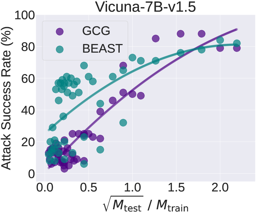
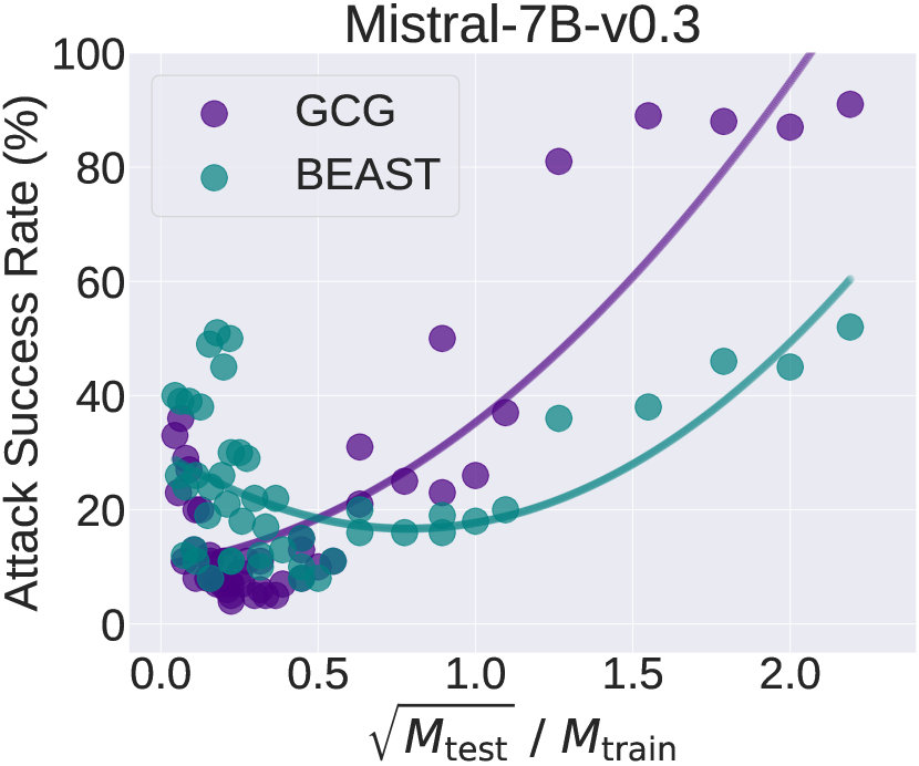
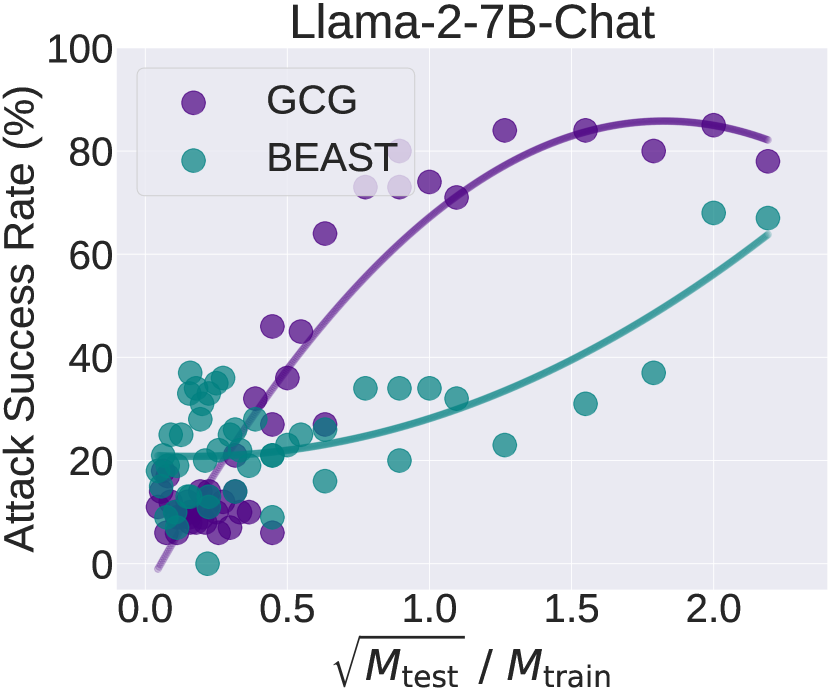
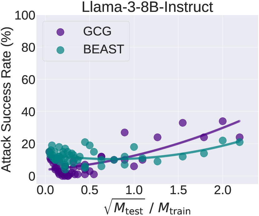
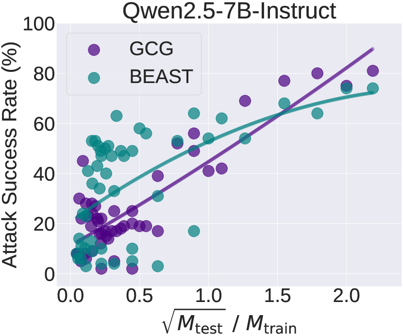
Figure 1: Scatter plots of ASR to the ratio of the square root of the adversarial token suffix length in jailbreak attacks to the adversarial token suffix length during AT (i.e., $\sqrt{M_{\text{test}}}/M_{\text{train}}$). For each pair of base model and attack, $48$ points are plotted. A high ASR indicates a weak jailbreak robustness of the model.

Table 1: PCCs and $p$-values calculated between ASR and the ratio $\sqrt{M_{\text{test}}}/M_{\text{train}}$. A high PCC (within the range $[-1,1]$) indicate a strong correlation between ASR and the ratio.

Model	GCG Attack		BEAST Attack
	PCC ($\uparrow$)	$p$-value ($\downarrow$)	PCC ($\uparrow$)	$p$-value ($\downarrow$)
Vicuna-7B	$0.93$	$4.70\times 10^{-21}$	$0.63$	$1.43\times 10^{-6}$
Mistral-7B	$0.86$	$3.97\times 10^{-15}$	$0.29$	$4.41\times 10^{-2}$
Llama-2-7B	$0.88$	$9.04\times 10^{-17}$	$0.68$	$1.32\times 10^{-7}$
Llama-3-8B	$0.76$	$2.75\times 10^{-10}$	$0.26$	$7.67\times 10^{-2}$
Qwen2.5-7B	$0.87$	$1.06\times 10^{-15}$	$0.58$	$1.03\times 10^{-5}$

Correlation between the jailbreak robustness and the ratio of the square root of the jailbreak adversarial suffix length to the adversarial suffix length in AT (i.e., $\sqrt{M_{\text{test}}}/M_{\text{train}}$). We plot the ASR of models trained and attacked with different adversarial suffix lengths in Figure 1. This results in $48$ points for each pair of base model and jailbreak attack. We also calculate the Pearson correlation coefficient (PCC) and the corresponding $p$-value between the ratio $\sqrt{M_{\text{test}}}/M_{\text{train}}$ and the ASR, as shown in Table 1.

When the jailbreak attack used during AT is the same as that used during robustness evaluation (i.e., GCG), one can observe from Figure 1 that a clear positive correlation between the ratio $\sqrt{M_{\text{test}}}/M_{\text{train}}$ and the ASR for all evaluated base models. Further, high PCCs ($>0.7$) and low $p$-values ($<0.05$) in Table 1 also confirm that the observed correlation is statistically significant.

However, when the jailbreak attack in AT is different from that in robustness evaluation (i.e., BEAST), from Table 1, the correlation between the ratio $\sqrt{M_{\text{test}}}/M_{\text{train}}$ and the ASR can only be observed from some of the base models (i.e., Vicuna-7B, Llama-2-7B, and Qwen2.5-7B) but not others. This may be due to the fact that AT with only a single jailbreak attack may not help the model generalize well to unseen attacks. Therefore, it might be necessary to adopt multiple attacks when performing AT-based alignment on LLMs. Nevertheless, from Figure 1, we find that for those models where the correlation between the ratio and ASR is not significant (i.e., Mistral-7B, and Llama-3-8B), GCG-based AT can still suppress the ASR to no more than $50\%$. This indicates that single-attack AT can still help models gain a certain degree of robustness against unseen attacks.

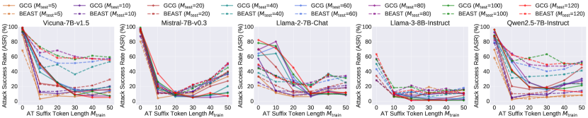
Figure 2: Curves of the ASR versus the adversarial suffix token length during AT (i.e., $M_{\text{train}}$) under jailbreak attacks with different adversarial suffix token lengths (i.e., $M_{\text{test}}$). $M_{\text{train}}=0$ means that AT is not performed on the evaluated model. A high ASR indicates a weak jailbreak robustness of the model.

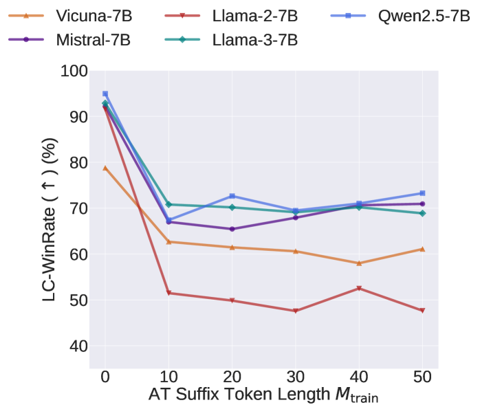
Figure 3: Utility analysis based on LC-WinRate. A high LC-WinRate indicates strong model utility. An LC-WinRate of $50\%$ means that the evaluated model has the same quality as the reference model Davinci003.

Relationship between adversarial suffix lengths in AT (i.e., $M_{\text{train}}$) and jailbreaking (i.e., $M_{\text{test}}$). We further plot curves of the model ASR versus the adversarial suffix token length during AT in Figure 2. From the figure, we find that as the adversarial suffix token length increases, AT can effectively reduce the ASR of both GCG and BEAST attacks. Furthermore, when the AT adversarial suffix token length is set to $20$, AT is already able to reduce the ASR by at least $30\%$ under all settings. Besides, it is worth noting that the adversarial suffix length during AT is only up to $50$, while that during jailbreaking can vary from $5$ to $120$. All these results suggest the effectiveness of defending against long-length jailbreaking with short-length AT.

Utility analysis. We plot the LC-WinRate of models trained under different adversarial suffix token lengths and the original pre-trained model (i.e., $M_{\text{train}}=0$) in Figure 3. We find that while AT reduces the utility of models, they can still achieve WinRates close to or more than $50\%$ against the reference Davinci003. This means that these adversarially trained models achieve utility comparable to Davinci003.

6 Conclusion

This paper studies the AT problem in LLMs and unveils that to defend against a suffix jailbreak attack with suffix length of $\Theta(M)$, it is sufficient to perform AT on adversarial prompts with suffix length of $\Theta(\sqrt{M})$. The finding is supported by both theoretical and empirical evidence. Theoretically, we define a new AT problem in the ICL theory and prove a robust generalization upper bound for adversarially trained linear transformers. This bound has a positive correlation with $\Theta(\sqrt{M_{\text{test}}}/M_{\text{train}})$. Empirically, we conduct AT on real-world LLMs and confirm a clear positive correlation between jailbreak ASR and ratio $\sqrt{M_{\text{test}}}/M_{\text{train}}$. Our results show that it is possible to conduct efficient “short-length” AT, which requires less GPU memory and training time, against strong “long-length” jailbreak attacks.

Appendix A Proofs

This section collects all the proofs in this paper.

A.1 Technical Lemmas

This section presents several technical lemmas that will be used in our proofs.

Lemma 1 (c.f. Lemma D.2 in Zhang et al. (2024)).

If $x\in\mathbb{R}^{d\times 1}$ is Gaussian random vector of $d$ dimension, mean zero and covariance matrix $\Lambda$, and $A\in\mathbb{R}^{d\times d}$ is a fixed matrix. Then

$$\mathop{\mathbb{E}}[xx^{\top}Axx^{\top}]=\Lambda(A+A^{\top})\Lambda+\mathrm{Tr}(A\Lambda)\Lambda.$$

Lemma 2.

If $x\in\mathbb{R}^{d\times 1}$ is Gaussian random vector of $d$ dimension, mean zero and covariance matrix $\Lambda$, and $A\in\mathbb{R}^{d\times d}$ is a fixed matrix. Then

$$\mathop{\mathbb{E}}[x^{\top}Ax]=\mathrm{Tr}(A\Lambda).$$

Proof.

Since

$$\mathop{\mathbb{E}}[x^{\top}Ax]=\mathop{\mathbb{E}}\Bigl{[}\sum_{i,j}x_{i}A_{i,j}x_{j}\Bigr{]}=\sum_{i,j}A_{i,j}\cdot\mathop{\mathbb{E}}[x_{i}x_{j}]=\sum_{i,j}A_{i,j}\cdot\Lambda_{i,j}=\sum_{i=1}^{d}(A\Lambda^{\top})_{i,i}=\mathrm{Tr}(A\Lambda),$$

which completes the proof. ∎

Lemma 3.

For any matrices $A\in\mathbb{R}^{n\times m}$ and $B\in\mathbb{R}^{m\times n}$, we have

$$\mathrm{Tr}(AB)=\mathrm{Tr}(BA).$$

Proof.

Since

$$\mathrm{Tr}(AB)=\sum_{i=1}^{n}(AB)_{i,i}=\sum_{i=1}^{n}\sum_{j=1}^{m}A_{i,j}B_{j,i}=\sum_{j=1}^{m}\sum_{i=1}^{n}B_{j,i}A_{i,j}=\sum_{j=1}^{m}(BA)_{j,j}=\mathrm{Tr}(BA),$$

which completes the proof. ∎

Lemma 4 (From Lemma D.1 in Zhang et al. (2024); Also in Petersen et al. (2008)).

Let $X\in\mathbb{R}^{n\times m}$ be a variable matrix and $A\in\mathbb{R}^{a\times n}$ and $B\in\mathbb{R}^{n\times m}$ be two fixed matrices. Then, we have

$$\partial_{X}\mathrm{Tr}(BX^{\top})=B\in\mathbb{R}^{n\times m},$$

$$\partial_{X}\mathrm{Tr}(AXBX^{\top})=(AXB+A^{\top}XB^{\top})\in\mathbb{R}^{n\times m}.$$

Lemma 5 (Von Neumann’s Trace Inequality; Also in Lemma D.3 in Zhang et al. (2024)).

Let $A\in\mathbb{R}^{n\times m}$ and $B\in\mathbb{R}^{m\times n}$ be two matrices. Suppose $\sigma_{1}(A)\leq\cdots\leq\sigma_{\min\{n,m\}}(A)$ and $\sigma_{1}(B)\leq\cdots\leq\sigma_{\min\{n,m\}}(B)$ are all the (ordered) singular values of $A$ and $B$, respectively. We have

$$\mathrm{Tr}(AB)\leq\sum_{i=1}^{\min\{n,m\}}\sigma_{i}(A)\sigma_{i}(B)\leq\sum_{i=1}^{\min\{n,m\}}\|A\|_{2}\cdot\|B\|_{2}=\min\{n,m\}\cdot\|A\|_{2}\cdot\|B\|_{2}.$$

A.2 Proof of Proposition 1

This section presents the proof of Proposition 1.

Proof of Proposition 1.

For the AT loss $\mathcal{L}(\theta)$ defined in Eq. (4.5), we have that

$$\mathcal{L}^{\text{adv}}(\theta):= \mathcal{R}^{\text{adv}}(\theta,M_{\text{train}})=\mathop{\mathbb{E}}_{\tau}\max_{\|\Delta_{\tau}^{\top}\|_{2,\infty}\leq\epsilon}|\hat{y}_{q,\theta}(E^{\text{adv}}_{\tau,M_{\text{train}}})-y_{\tau,q}|^{2}$$

$$= \mathop{\mathbb{E}}_{\tau}\left\{\max_{\|\Delta_{\tau}^{\top}\|_{2,\infty}\leq\epsilon}\frac{1}{2}\left|\begin{pmatrix}(w^{V}_{21})^{\top}&w^{V}_{22}\end{pmatrix}\cdot\frac{E^{\text{adv}}_{\tau,M_{\text{train}}}E^{\text{adv},\top}_{\tau,M_{\text{train}}}}{N+M_{\text{train}}}\cdot\begin{pmatrix}W^{KQ}_{11}\\ (w^{KQ}_{21})^{\top}\end{pmatrix}\cdot x_{\tau,q}-y_{\tau,q}\right|^{2}\right\}.$$ (A.1)

Then, the term $E^{\text{adv}}_{\tau,M_{\text{train}}}E^{\text{adv},\top}_{\tau,M_{\text{train}}}$ can be decomposed as follows,

$$E^{\text{adv}}_{\tau,M_{\text{train}}}E^{\text{adv},\top}_{\tau,M_{\text{train}}}=\begin{pmatrix}\begin{pmatrix}X_{\tau}\\ Y_{\tau}\end{pmatrix}&\begin{pmatrix}X^{\text{sfx}}_{\tau}+\Delta_{\tau}\\ Y^{\text{sfx}}_{\tau}\end{pmatrix}&\begin{pmatrix}x_{\tau,q}\\ 0\end{pmatrix}\end{pmatrix}\cdot\begin{pmatrix}\begin{pmatrix}X_{\tau}\\ Y_{\tau}\end{pmatrix}&\begin{pmatrix}X^{\text{sfx}}_{\tau}+\Delta_{\tau}\\ Y^{\text{sfx}}_{\tau}\end{pmatrix}&\begin{pmatrix}x_{\tau,q}\\ 0\end{pmatrix}\end{pmatrix}^{\top}$$

$$=\begin{pmatrix}X_{\tau}&X^{\text{sfx}}_{\tau}&x_{\tau,q}\\ Y_{\tau}&Y^{\text{sfx}}_{\tau}&0\end{pmatrix}\begin{pmatrix}X_{\tau}&X^{\text{sfx}}_{\tau}&x_{\tau,q}\\ Y_{\tau}&Y^{\text{sfx}}_{\tau}&0\end{pmatrix}^{\top}+\begin{pmatrix}0_{d\times N}&\Delta_{\tau}&0_{d\times 1}\\ 0_{1\times N}&0_{1\times M_{\text{train}}}&0\end{pmatrix}\begin{pmatrix}0_{d\times N}&\Delta_{\tau}&0_{d\times 1}\\ 0_{1\times N}&0_{1\times M_{\text{train}}}&0\end{pmatrix}^{\top}$$

$$\quad\quad+\begin{pmatrix}X_{\tau}&X^{\text{sfx}}_{\tau}&x_{\tau,q}\\ Y_{\tau}&Y^{\text{sfx}}_{\tau}&0\end{pmatrix}\begin{pmatrix}0_{d\times N}&\Delta_{\tau}&0_{d\times 1}\\ 0_{1\times N}&0_{1\times M_{\text{train}}}&0\end{pmatrix}^{\top}+\begin{pmatrix}0_{d\times N}&\Delta_{\tau}&0_{d\times 1}\\ 0_{1\times N}&0_{1\times M_{\text{train}}}&0\end{pmatrix}\begin{pmatrix}X_{\tau}&X^{\text{sfx}}_{\tau}&x_{\tau,q}\\ Y_{\tau}&Y^{\text{sfx}}_{\tau}&0\end{pmatrix}^{\top}$$

$$=\begin{pmatrix}X_{\tau}&X^{\text{sfx}}_{\tau}&x_{\tau,q}\\ Y_{\tau}&Y^{\text{sfx}}_{\tau}&0\end{pmatrix}\begin{pmatrix}X_{\tau}&X^{\text{sfx}}_{\tau}&x_{\tau,q}\\ Y_{\tau}&Y^{\text{sfx}}_{\tau}&0\end{pmatrix}^{\top}+\begin{pmatrix}\Delta_{\tau}\\ 0_{1\times M_{\text{train}}}\end{pmatrix}\begin{pmatrix}\Delta_{\tau}\\ 0_{1\times M_{\text{train}}}\end{pmatrix}^{\top}+\begin{pmatrix}X^{\text{sfx}}_{\tau}\\ Y^{\text{sfx}}_{\tau}\end{pmatrix}\begin{pmatrix}\Delta_{\tau}\\ 0_{1\times M_{\text{train}}}\end{pmatrix}^{\top}+\begin{pmatrix}\Delta_{\tau}\\ 0_{1\times M_{\text{train}}}\end{pmatrix}\begin{pmatrix}X^{\text{sfx}}_{\tau}\\ Y^{\text{sfx}}_{\tau}\end{pmatrix}^{\top},$$

which further means that

$$\begin{pmatrix}(w^{V}_{21})^{\top}&w^{V}_{22}\end{pmatrix}\cdot\frac{E^{\text{adv}}_{\tau,M_{\text{train}}}E^{\text{adv},\top}_{\tau,M_{\text{train}}}}{N+M_{\text{train}}}\cdot\begin{pmatrix}W^{KQ}_{11}\\ (w^{KQ}_{21})^{\top}\end{pmatrix}\cdot x_{\tau,q}$$

$$=\begin{pmatrix}(w^{V}_{21})^{\top}&w^{V}_{22}\end{pmatrix}\cdot\frac{\begin{pmatrix}X_{\tau}&X^{\text{sfx}}_{\tau}&x_{\tau,q}\\ Y_{\tau}&Y^{\text{sfx}}_{\tau}&0\end{pmatrix}\begin{pmatrix}X_{\tau}&X^{\text{sfx}}_{\tau}&x_{\tau,q}\\ Y_{\tau}&Y^{\text{sfx}}_{\tau}&0\end{pmatrix}^{\top}}{N+M_{\text{train}}}\cdot\begin{pmatrix}W^{KQ}_{11}\\ (w^{KQ}_{21})^{\top}\end{pmatrix}\cdot x_{\tau,q}+(w^{V}_{21})^{\top}\cdot\frac{\Delta_{\tau}\Delta_{\tau}^{\top}}{N+M_{\text{train}}}\cdot W^{KQ}_{11}x_{\tau,q}$$

$$\quad\quad+\begin{pmatrix}(w^{V}_{21})^{\top}&w^{V}_{22}\end{pmatrix}\cdot\frac{\begin{pmatrix}X^{\text{sfx}}_{\tau}\\ Y^{\text{sfx}}_{\tau}\end{pmatrix}\Delta_{\tau}^{\top}}{N+M_{\text{train}}}\cdot W^{KQ}_{11}x_{\tau,q}+(w^{V}_{21})^{\top}\cdot\frac{\Delta_{\tau}\begin{pmatrix}X^{\text{sfx}}_{\tau}\\ Y^{\text{sfx}}_{\tau}\end{pmatrix}^{\top}}{N+M_{\text{train}}}\cdot\begin{pmatrix}W^{KQ}_{11}\\ (w^{KQ}_{21})^{\top}\end{pmatrix}x_{\tau,q}.$$ (A.2)

Inserting Eq. (A.2) into Eq. (A.1) and applying the inequality that $|a+b|^{2}\leq 2\cdot(a^{2}+b^{2})$, $\mathcal{L}^{\text{adv}}(\theta)$ can thus be bounded as

$$\mathcal{L}^{\text{adv}}(\theta) \leq 2\cdot\mathop{\mathbb{E}}_{\tau}\Bigl{[}\begin{pmatrix}(w^{V}_{21})^{\top}&w^{V}_{22}\end{pmatrix}\cdot\frac{\begin{pmatrix}X_{\tau}&X^{\text{sfx}}_{\tau}&x_{\tau,q}\\ Y_{\tau}&Y^{\text{sfx}}_{\tau}&0\end{pmatrix}\begin{pmatrix}X_{\tau}&X^{\text{sfx}}_{\tau}&x_{\tau,q}\\ Y_{\tau}&Y^{\text{sfx}}_{\tau}&0\end{pmatrix}^{\top}}{N+M_{\text{train}}}\cdot\begin{pmatrix}W^{KQ}_{11}\\ (w^{KQ}_{21})^{\top}\end{pmatrix}\cdot x_{\tau,q}-y_{\tau,q}\Bigr{]}^{2}$$

$$\quad+\underbrace{2\cdot\mathop{\mathbb{E}}_{\tau}\max_{\|\Delta_{\tau}^{\top}\|_{2,\infty}\leq\epsilon}\Bigl{[}(w^{V}_{21})^{\top}\cdot\frac{\Delta_{\tau}\Delta_{\tau}^{\top}}{N+M_{\text{train}}}\cdot W^{KQ}_{11}x_{\tau,q}\Bigr{]}^{2}}_{:=A_{1}(\theta)}$$

$$\quad+\underbrace{2\cdot\mathop{\mathbb{E}}_{\tau}\max_{\|\Delta_{\tau}^{\top}\|_{2,\infty}\leq\epsilon}\Bigl{[}\begin{pmatrix}(w^{V}_{21})^{\top}&w^{V}_{22}\end{pmatrix}\cdot\frac{\begin{pmatrix}X^{\text{sfx}}_{\tau}\\ Y^{\text{sfx}}_{\tau}\end{pmatrix}\Delta_{\tau}^{\top}}{N+M_{\text{train}}}\cdot W^{KQ}_{11}x_{\tau,q}\Bigr{]}^{2}}_{:=A_{2}(\theta)}$$

$$\quad+\underbrace{2\cdot\mathop{\mathbb{E}}_{\tau}\max_{\|\Delta_{\tau}^{\top}\|_{2,\infty}\leq\epsilon}\Bigl{[}(w^{V}_{21})^{\top}\cdot\frac{\Delta_{\tau}\begin{pmatrix}X^{\text{sfx}}_{\tau}\\ Y^{\text{sfx}}_{\tau}\end{pmatrix}^{\top}}{N+M_{\text{train}}}\cdot\begin{pmatrix}W^{KQ}_{11}\\ (w^{KQ}_{21})^{\top}\end{pmatrix}x_{\tau,q}\Bigr{]}^{2}}_{:=A_{3}(\theta)}.$$ (A.3)

We then bound terms $A_{1}(\theta)$, $A_{2}(\theta)$, and $A_{3}(\theta)$ in Eq. (A.3) seprately. For the term $A_{1}(\theta)$ in Eq. (A.3), we have

$$A_{1}(\theta):=\frac{2}{(N+M_{\text{train}})^{2}}\cdot\mathop{\mathbb{E}}_{\tau}\max_{\|\Delta_{\tau}^{\top}\|_{2,\infty}\leq\epsilon}\Bigl{[}(w^{V}_{21})^{\top}\cdot\sum_{i=1}^{M_{\text{train}}}\delta_{\tau,i}\delta_{\tau,i}^{\top}\cdot W^{KQ}_{11}x_{\tau,q}\Bigr{]}^{2}$$

$$\leq\frac{2}{(N+M_{\text{train}})^{2}}\cdot\mathop{\mathbb{E}}_{\tau}\max_{\|\Delta_{\tau}^{\top}\|_{2,\infty}\leq\epsilon}\Bigl{[}\underbrace{\sum_{i=1}^{M_{\text{train}}}[(w^{V}_{21})^{\top}\delta_{\tau,i}]^{2}\cdot\sum_{i=1}^{M_{\text{train}}}[\delta_{\tau,i}^{\top}W^{KQ}_{11}x_{\tau,q}]^{2}}_{\text{by Cauchy-Schwarz Inequality}}\Bigr{]}$$

$$\leq\frac{2}{(N+M_{\text{train}})^{2}}\cdot\mathop{\mathbb{E}}_{\tau}\Bigl{[}\sum_{i=1}^{M_{\text{train}}}\max_{\|\delta_{\tau,i}\|_{2}\leq\epsilon}[(w^{V}_{21})^{\top}\delta_{\tau,i}]^{2}\cdot\sum_{i=1}^{M_{\text{train}}}\max_{\|\delta_{\tau,i}\|_{2}\leq\epsilon}[\delta_{i}^{\top}W^{KQ}_{11}x_{\tau,q}]^{2}\Bigr{]}$$

$$=\frac{2}{(N+M_{\text{train}})^{2}}\cdot\mathop{\mathbb{E}}_{\tau}\Bigl{[}\sum_{i=1}^{M_{\text{train}}}[\|w^{V}_{21}\|_{2}\cdot\epsilon]^{2}\cdot\sum_{i=1}^{M_{\text{train}}}[\|W^{KQ}_{11}x_{\tau,q}\|_{2}\cdot\epsilon]^{2}\Bigr{]}$$

$$=\frac{2\epsilon^{4}M_{\text{train}}^{2}}{(N+M_{\text{train}})^{2}}\cdot\|w^{V}_{21}\|_{2}^{2}\cdot\mathop{\mathbb{E}}_{\tau}\|W^{KQ}_{11}x_{\tau,q}\|_{2}^{2}.$$ (A.4)

For the term $A_{2}(\theta)$ in Eq. (A.3), we have

$$A_{2}(\theta):=\frac{2}{(N+M_{\text{train}})^{2}}\cdot\mathop{\mathbb{E}}_{\tau}\max_{\|\Delta_{\tau}^{\top}\|_{2,\infty}\leq\epsilon}\Bigl{[}\begin{pmatrix}(w^{V}_{21})^{\top}&w^{V}_{22}\end{pmatrix}\cdot\sum_{i=1}^{M_{\text{train}}}\begin{pmatrix}x^{\text{sfx}}_{\tau,i}\\ y^{\text{sfx}}_{\tau,i}\end{pmatrix}\delta_{\tau,i}^{\top}\cdot W^{KQ}_{11}x_{\tau,q}\Bigr{]}^{2}$$

$$\leq\frac{2}{(N+M_{\text{train}})^{2}}\cdot\mathop{\mathbb{E}}_{\tau}\max_{\|\Delta_{\tau}^{\top}\|_{2,\infty}\leq\epsilon}\Bigl{[}\underbrace{\sum_{i=1}^{M_{\text{train}}}\Bigl{[}\begin{pmatrix}(w^{V}_{21})^{\top}&w^{V}_{22}\end{pmatrix}\begin{pmatrix}x^{\text{sfx}}_{\tau,i}\\ y^{\text{sfx}}_{\tau,i}\end{pmatrix}\Bigr{]}^{2}\cdot\sum_{i=1}^{M_{\text{train}}}[\delta_{\tau,i}^{\top}W^{KQ}_{11}x_{\tau,q}]^{2}}_{\text{by Cauchy-Schwarz Inequality}}\Bigr{]}$$

$$=\frac{2}{(N+M_{\text{train}})^{2}}\cdot\sum_{i=1}^{M_{\text{train}}}\mathop{\mathbb{E}}_{\tau}\Bigl{[}\begin{pmatrix}(w^{V}_{21})^{\top}&w^{V}_{22}\end{pmatrix}\begin{pmatrix}x^{\text{sfx}}_{\tau,i}\\ y^{\text{sfx}}_{\tau,i}\end{pmatrix}\Bigr{]}^{2}\cdot\sum_{i=1}^{M_{\text{train}}}\mathop{\mathbb{E}}_{\tau}\Bigl{[}\max_{\|\delta_{\tau,i}\|_{2}\leq\epsilon}[\delta_{\tau,i}^{\top}W^{KQ}_{11}x_{\tau,q}]^{2}\Bigr{]}$$

$$=\frac{2}{(N+M_{\text{train}})^{2}}\cdot\sum_{i=1}^{M_{\text{train}}}\mathop{\mathbb{E}}_{\tau}\Bigl{[}\begin{pmatrix}(w^{V}_{21})^{\top}&w^{V}_{22}\end{pmatrix}\begin{pmatrix}x^{\text{sfx}}_{\tau,i}\\ y^{\text{sfx}}_{\tau,i}\end{pmatrix}\Bigr{]}^{2}\cdot\sum_{i=1}^{M_{\text{train}}}\mathop{\mathbb{E}}_{\tau}[\|W^{KQ}_{11}x_{\tau,q}\|_{2}\cdot\epsilon]^{2}$$

$$=\frac{2\epsilon^{2}M_{\text{train}}}{(N+M_{\text{train}})^{2}}\cdot\mathop{\mathbb{E}}_{\tau}\|W^{KQ}_{11}x_{\tau,q}\|_{2}^{2}\cdot\sum_{i=1}^{M_{\text{train}}}\mathop{\mathbb{E}}_{\tau}\Bigl{[}\begin{pmatrix}(w^{V}_{21})^{\top}&w^{V}_{22}\end{pmatrix}\begin{pmatrix}x^{\text{sfx}}_{\tau,i}\\ y^{\text{sfx}}_{\tau,i}\end{pmatrix}\Bigr{]}^{2}.$$ (A.5)

For the term $A_{3}(\theta)$ in Eq. (A.3), we have

$$A_{3}(\theta):=\frac{2}{(N+M_{\text{train}})^{2}}\cdot\mathop{\mathbb{E}}_{\tau}\max_{\|\Delta_{\tau}^{\top}\|_{2,\infty}\leq\epsilon}\Bigl{[}(w^{V}_{21})^{\top}\cdot\sum_{i=1}^{M_{\text{train}}}\delta_{\tau,i}\begin{pmatrix}x^{\text{sfx}}_{\tau,i}\\ y^{\text{sfx}}_{\tau,i}\end{pmatrix}^{\top}\cdot\begin{pmatrix}W^{KQ}_{11}\\ (w^{KQ}_{21})^{\top}\end{pmatrix}x_{\tau,q}\Bigr{]}^{2}$$

$$\leq\frac{2}{(N+M_{\text{train}})^{2}}\cdot\mathop{\mathbb{E}}_{\tau}\max_{\|\Delta_{\tau}^{\top}\|_{2,\infty}\leq\epsilon}\Bigl{[}\underbrace{\sum_{i=1}^{M_{\text{train}}}[(w^{V}_{21})^{\top}\delta_{\tau,i}]^{2}\cdot\sum_{i=1}^{M_{\text{train}}}\Bigl{[}\begin{pmatrix}x^{\text{sfx}}_{\tau,i}\\ y^{\text{sfx}}_{\tau,i}\end{pmatrix}^{\top}\begin{pmatrix}W^{KQ}_{11}\\ (w^{KQ}_{21})^{\top}\end{pmatrix}x_{\tau,q}\Bigr{]}^{2}}_{\text{by Cauchy-Schwarz Inequality}}\Bigr{]}$$

$$=\frac{2}{(N+M_{\text{train}})^{2}}\cdot\mathop{\mathbb{E}}_{\tau}\Bigl{[}\sum_{i=1}^{M_{\text{train}}}\max_{\|\delta_{\tau,i}\|_{2}\leq\epsilon}[(w^{V}_{21})^{\top}\delta_{\tau,i}]^{2}\cdot\sum_{i=1}^{M_{\text{train}}}\Bigl{[}\begin{pmatrix}x^{\text{sfx}}_{\tau,i}\\ y^{\text{sfx}}_{\tau,i}\end{pmatrix}^{\top}\begin{pmatrix}W^{KQ}_{11}\\ (w^{KQ}_{21})^{\top}\end{pmatrix}x_{\tau,q}\Bigr{]}^{2}\Bigr{]}$$

$$=\frac{2}{(N+M_{\text{train}})^{2}}\cdot\mathop{\mathbb{E}}_{\tau}\Bigl{[}\sum_{i=1}^{M_{\text{train}}}[\|w^{V}_{21}\|_{2}\cdot\epsilon]^{2}\cdot\sum_{i=1}^{M_{\text{train}}}\Bigl{[}\begin{pmatrix}x^{\text{sfx}}_{\tau,i}\\ y^{\text{sfx}}_{\tau,i}\end{pmatrix}^{\top}\begin{pmatrix}W^{KQ}_{11}\\ (w^{KQ}_{21})^{\top}\end{pmatrix}x_{\tau,q}\Bigr{]}^{2}\Bigr{]}$$

$$=\frac{2\epsilon^{2}M_{\text{train}}}{(N+M_{\text{train}})^{2}}\cdot\|w^{V}_{21}\|_{2}^{2}\cdot\sum_{i=1}^{M_{\text{train}}}\mathop{\mathbb{E}}_{\tau}\Bigl{[}\begin{pmatrix}x^{\text{sfx}}_{\tau,i}\\ y^{\text{sfx}}_{\tau,i}\end{pmatrix}^{\top}\begin{pmatrix}W^{KQ}_{11}\\ (w^{KQ}_{21})^{\top}\end{pmatrix}x_{\tau,q}\Bigr{]}^{2}.$$ (A.6)

As a result, by inserting Eqs. (A.4), (A.5), and (A.6) into Eq. (A.3), we finally have that

$$\mathcal{L}^{\text{adv}}(\theta) \leq 2\cdot\mathop{\mathbb{E}}_{\tau}\Bigl{[}\begin{pmatrix}(w^{V}_{21})^{\top}&w^{V}_{22}\end{pmatrix}\cdot\frac{\begin{pmatrix}X_{\tau}&X^{\text{sfx}}_{\tau}&x_{\tau,q}\\ Y_{\tau}&Y^{\text{sfx}}_{\tau}&0\end{pmatrix}\begin{pmatrix}X_{\tau}&X^{\text{sfx}}_{\tau}&x_{\tau,q}\\ Y_{\tau}&Y^{\text{sfx}}_{\tau}&0\end{pmatrix}^{\top}}{N+M_{\text{train}}}\cdot\begin{pmatrix}W^{KQ}_{11}\\ (w^{KQ}_{21})^{\top}\end{pmatrix}\cdot x_{\tau,q}-y_{\tau,q}\Bigr{]}^{2}$$

$$\quad+\frac{2\epsilon^{4}M_{\text{train}}^{2}}{(N+M_{\text{train}})^{2}}\cdot\|w^{V}_{21}\|_{2}^{2}\cdot\mathop{\mathbb{E}}_{\tau}\|W^{KQ}_{11}x_{\tau,q}\|_{2}^{2}$$

$$\quad+\frac{2\epsilon^{2}M_{\text{train}}}{(N+M_{\text{train}})^{2}}\cdot\mathop{\mathbb{E}}_{\tau}\|W^{KQ}_{11}x_{\tau,q}\|_{2}^{2}\cdot\sum_{i=1}^{M_{\text{train}}}\mathop{\mathbb{E}}_{\tau}\Bigl{[}\begin{pmatrix}(w^{V}_{21})^{\top}&w^{V}_{22}\end{pmatrix}\begin{pmatrix}x^{\text{sfx}}_{\tau,i}\\ y^{\text{sfx}}_{\tau,i}\end{pmatrix}\Bigr{]}^{2}$$

$$\quad+\frac{2\epsilon^{2}M_{\text{train}}}{(N+M_{\text{train}})^{2}}\cdot\|w^{V}_{21}\|_{2}^{2}\cdot\sum_{i=1}^{M_{\text{train}}}\mathop{\mathbb{E}}_{\tau}\Bigl{[}\begin{pmatrix}x^{\text{sfx}}_{\tau,i}\\ y^{\text{sfx}}_{\tau,i}\end{pmatrix}^{\top}\begin{pmatrix}W^{KQ}_{11}\\ (w^{KQ}_{21})^{\top}\end{pmatrix}x_{\tau,q}\Bigr{]}^{2}.$$ (A.7)

The right-hand-side of Eq. (A.7) is exactly the surrogate AT loss $\tilde{\mathcal{L}}^{\text{adv}}(\theta)$ in Eq. (4.6), which thus completes the proof. ∎

A.3 Proof of Theorem 1

This section presents the proof of Theorem 1, which is inspired by that in Zhang et al. (2024). Specifically:

1. we first prove that terms $w^{V}_{21}$ and $w^{KQ}_{21}$ stay zero during the surrogate AT (Lemma 6) via continuous gradient-flow, which thus can simplify the surrogate AT loss $\tilde{\mathcal{L}}^{\text{adv}}(\theta)$ defined in Eq. (4.6) (Lemma 7).

2. We then calculate a closed-form solution $\theta_{*}$ for the surrogate AT problem based on the simplified $\tilde{\mathcal{L}}^{\text{adv}}(\theta)$ (Lemma 8), which is exactly the solution given in Theorem 1.

3. Finally, we prove that under the continuous gradient flow, the LSA model starts from the initial point defined in Assumption 1 can indeed converge to the closed-form solution $\theta_{*}$ (Lemma 12), which thus completes the proof of Theorem 1.

We now start to prove the following Lemma 6.

Lemma 6.

Suppose Assumption 1 holds and the LSA model $f_{\text{\rm LSA},\theta}$ is trained via minimizing surrogate AT loss $\tilde{\mathcal{L}}^{\text{\rm adv}}(\theta)$ in Eq. (4.6) with continuous gradient flow. Then, for any continuous training time $t\geq 0$, we uniformly have that $w^{V}_{21}(t)=w^{KQ}_{21}(t)=0_{d\times 1}$.

Proof.

When the LSA model $f_{\text{LSA},\theta}$ is trained with continuous gradient-flow, the updates of $w^{V}_{21}$ and $w^{KQ}_{21}$ with respect to the continuous training time $t\geq 0$ are given by

$$\partial_{t}w^{V}_{21}(t):=-\partial_{w^{V}_{21}}\tilde{\mathcal{L}}^{\text{adv}}(\theta),$$

$$\partial_{t}w^{KQ}_{21}(t):=-\partial_{w^{KQ}_{21}}\tilde{\mathcal{L}}^{\text{adv}}(\theta).$$

Meanwhile, since Assumption 1 assumes that $w^{V}_{21}(0)=W^{KQ}_{21}(0)=0_{d\times 1}$, therefore, to complete the proof, we only need to show that $\partial_{t}w^{V}_{21}(t)=\partial_{t}W^{KQ}_{21}(t)=0_{1\times d}$ as long as $w^{V}_{21}(t)=W^{KQ}_{21}(t)=0_{d\times 1}$ for any $t\geq 0$. In other words, below we need to show that $w^{V}_{21}=W^{KQ}_{21}=0_{d\times 1}$ indicates $\partial_{w^{V}_{21}}\tilde{\mathcal{L}}^{\text{adv}}(\theta)=\partial_{w^{KQ}_{21}}\tilde{\mathcal{L}}^{\text{adv}}(\theta)=0_{1\times d}$.

Toward this end, we adopt the notation in Eq. (4.6) to decompose the surrogate AT loss $\tilde{\mathcal{L}}(\theta)$ as follows,

$$\tilde{\mathcal{L}}^{\text{adv}}(\theta):=[\ell_{1}(\theta)+\ell_{2}(\theta)+\ell_{3}(\theta)+\ell_{4}(\theta)],$$

where

$$\ell_{1}(\theta)=2\mathop{\mathbb{E}}_{\tau}\Bigl{[}((w^{V}_{21})^{\top}\ \ w^{V}_{22})\frac{\begin{pmatrix}X_{\tau}&X^{\text{sfx}}_{\tau}&x_{\tau,q}\\ Y_{\tau}&Y^{\text{sfx}}_{\tau}&0\end{pmatrix}\begin{pmatrix}X_{\tau}&X^{\text{sfx}}_{\tau}&x_{\tau,q}\\ Y_{\tau}&Y^{\text{sfx}}_{\tau}&0\end{pmatrix}^{\top}}{N+M_{\text{train}}}\begin{pmatrix}W^{KQ}_{11}\\ (w^{KQ}_{21})^{\top}\end{pmatrix}x_{\tau,q}-y_{\tau,q}\Bigr{]}^{2},$$ (A.8)

$$\ell_{2}(\theta)=\frac{2\epsilon^{4}M_{\text{train}}^{2}}{(N+M_{\text{train}})^{2}}\|w^{V}_{21}\|_{2}^{2}\mathop{\mathbb{E}}_{\tau}\Bigl{[}\|W^{KQ}_{11}x_{\tau,q}\|_{2}^{2}\Bigr{]},$$ (A.9)

$$\ell_{3}(\theta)=\frac{2\epsilon^{2}M_{\text{train}}}{(N+M_{\text{train}})^{2}}\mathop{\mathbb{E}}_{\tau}\Bigl{[}\|W^{KQ}_{11}x_{\tau,q}\|_{2}^{2}\cdot\|((w^{V}_{21})^{\top}\ \ w^{V}_{22})\begin{pmatrix}X^{\text{sfx}}_{\tau}\\ Y^{\text{sfx}}_{\tau}\end{pmatrix}\|_{2}^{2}\Bigr{]},$$ (A.10)

$$\ell_{4}(\theta)=\frac{2\epsilon^{2}M_{\text{train}}}{(N+M_{\text{train}})^{2}}\|w^{V}_{21}\|_{2}^{2}\cdot\mathop{\mathbb{E}}_{\tau}\Bigl{[}\|\begin{pmatrix}X^{\text{sfx}}_{\tau}\\ Y^{\text{sfx}}_{\tau}\end{pmatrix}^{\top}\begin{pmatrix}W^{KQ}_{11}\\ (w^{KQ}_{21})^{\top}\end{pmatrix}x_{\tau,q}\|_{2}^{2}\Bigr{]}.$$ (A.11)

In the remaining of this proof, we will show that when $w^{V}_{21}=w^{KQ}_{21}=0_{d\times 1}$ holds, one has: (1) $\partial_{W^{V}_{21}}\ell_{1}(\theta)=\partial_{W^{KQ}_{21}}\ell_{1}(\theta)=0_{1\times d}$, (2) $\partial_{W^{V}_{21}}\ell_{2}(\theta)=\partial_{W^{KQ}_{21}}\ell_{2}(\theta)=0_{1\times d}$, (3) $\partial_{W^{V}_{21}}\ell_{3}(\theta)=\partial_{W^{KQ}_{21}}\ell_{3}(\theta)=0_{1\times d}$, and (4) $\partial_{W^{V}_{21}}\ell_{4}(\theta)=\partial_{W^{KQ}_{21}}\ell_{4}(\theta)=0_{1\times d}$, which thus automatically indicates that $\partial_{W^{V}_{21}}\tilde{\mathcal{L}}^{\text{adv}}(\theta)=\partial_{W^{KQ}_{21}}\tilde{\mathcal{L}}^{\text{adv}}(\theta)=0_{1\times d}$.

Step 1: Show that $w^{V}_{21}=w^{KQ}_{21}=0_{d\times 1}$ indicates $\partial_{W^{V}_{21}}\ell_{1}(\theta)=\partial_{W^{KQ}_{21}}\ell_{1}(\theta)=0_{1\times d}$. Such a claim can be directly obtained from the proofs in Zhang et al. (2024). Specifically, when setting the (original) ICL prompt length from $N$ to $(N+M_{\text{train}})$, the ICL training loss $L$ in Zhang et al. (2024) is equivalent to our $\ell_{1}(\theta)$ defined in Eq. (A.8). Therefore, one can then follow the same procedures as those in the proof of Lemma 5.2 in Zhang et al. (2024) to show that the continuous gradient flows of $W^{V}_{21}$ and $W^{KQ}_{21}$ are zero when Assumption 1 holds. Please refer accordingly for details.

Step 2: Show that $w^{V}_{21}=w^{KQ}_{21}=0_{d\times 1}$ indicates $\partial_{w^{V}_{21}}\ell_{2}(\theta)=\partial_{w^{KQ}_{21}}\ell_{2}(\theta)=0_{1\times d}$. Since the term $w^{KQ}_{21}$ does not exist in the expression of $\ell_{2}(\theta)$ in Eq. (A.9), we directly have that $\partial_{w^{KQ}_{21}}\ell_{2}(\theta)=0_{1\times d}$. Besides, for the derivative $\partial_{w^{V}_{21}}\ell_{2}(\theta)$, based on Eq. (A.9) we further have that

$$\left.\partial_{w^{V}_{21}}\ell_{2}(\theta)\right|_{w^{V}_{21}=0_{d\times 1}}=\partial_{w^{V}_{21}}\left.\Bigl{[}\frac{2\epsilon^{4}M_{\text{train}}^{2}}{(N+M_{\text{train}})^{2}}\cdot\|w^{V}_{21}\|_{2}^{2}\cdot\mathop{\mathbb{E}}_{\tau}\|W^{KQ}_{11}x_{\tau,q}\|_{2}^{2}\Bigr{]}\right|_{w^{V}_{21}=0_{d\times 1}}$$

$$=\left.\Bigl{[}\frac{4\epsilon^{4}M_{\text{train}}^{2}}{(N+M_{\text{train}})^{2}}\cdot\mathop{\mathbb{E}}_{\tau}\|W^{KQ}_{11}x_{\tau,q}\|_{2}^{2}\cdot(w^{V}_{21})^{\top}\Bigr{]}\right|_{w^{V}_{21}=0_{d\times 1}}$$

$$=\frac{4\epsilon^{4}M_{\text{train}}^{2}}{(N+M_{\text{train}})^{2}}\cdot\mathop{\mathbb{E}}_{\tau}\|W^{KQ}_{11}x_{\tau,q}\|_{2}^{2}\cdot 0_{d\times 1}^{\top}=0_{1\times d},$$

which justifies our claim in Step 2.

Step 3: Show that $w^{V}_{21}=w^{KQ}_{21}=0_{d\times 1}$ indicates $\partial_{w^{V}_{21}}\ell_{3}(\theta)=\partial_{w^{KQ}_{21}}\ell_{3}(\theta)=0_{1\times d}$. We first rewrite $\ell_{3}(\theta)$ that defined in Eq. (A.10) as follows,

$$\ell_{3}(\theta)=\frac{2\epsilon^{2}M_{\text{train}}}{(N+M_{\text{train}})^{2}}\mathop{\mathbb{E}}_{\tau}\Bigl{[}\|W^{KQ}_{11}x_{\tau,q}\|_{2}^{2}\cdot\|((w^{V}_{21})^{\top}\ \ w^{V}_{22})\begin{pmatrix}X^{\text{sfx}}_{\tau}\\ Y^{\text{sfx}}_{\tau}\end{pmatrix}\|_{2}^{2}\Bigr{]}$$

$$=\frac{2\epsilon^{2}M_{\text{train}}}{(N+M_{\text{train}})^{2}}\cdot\mathop{\mathbb{E}}_{\tau}\Bigl{[}\|W^{KQ}_{11}x_{\tau,q}\|_{2}^{2}\Bigr{]}\cdot\sum_{i=1}^{M_{\text{train}}}\mathop{\mathbb{E}}_{\tau}\Bigl{[}\begin{pmatrix}(w^{V}_{21})^{\top}&w^{V}_{22}\end{pmatrix}\cdot\begin{pmatrix}x^{\text{sfx}}_{\tau,i}\\ y^{\text{sfx}}_{\tau,i}\end{pmatrix}\begin{pmatrix}x^{\text{sfx}}_{\tau,i}\\ y^{\text{sfx}}_{\tau,i}\end{pmatrix}^{\top}\cdot\begin{pmatrix}(w^{V}_{21})^{\top}&w^{V}_{22}\end{pmatrix}^{\top}\Bigr{]}$$

$$=\frac{2\epsilon^{2}M_{\text{train}}}{(N+M_{\text{train}})^{2}}\cdot\mathop{\mathbb{E}}_{\tau}\Bigl{[}\|W^{KQ}_{11}x_{\tau,q}\|_{2}^{2}\Bigr{]}\cdot\begin{pmatrix}(w^{V}_{21})^{\top}&w^{V}_{22}\end{pmatrix}\cdot\left(\sum_{i=1}^{M_{\text{train}}}\mathop{\mathbb{E}}_{\tau}\Bigl{[}\begin{pmatrix}x^{\text{sfx}}_{\tau,i}\\ y^{\text{sfx}}_{\tau,i}\end{pmatrix}\begin{pmatrix}x^{\text{sfx}}_{\tau,i}\\ y^{\text{sfx}}_{\tau,i}\end{pmatrix}^{\top}\Bigr{]}\right)\cdot\begin{pmatrix}(w^{V}_{21})^{\top}&w^{V}_{22}\end{pmatrix}^{\top}.$$ (A.12)

Then, for any $i\in[M]$ we have

$$\mathop{\mathbb{E}}_{\tau}\Bigl{[}\begin{pmatrix}x^{\text{sfx}}_{\tau,i}\\ y^{\text{sfx}}_{\tau,i}\end{pmatrix}\begin{pmatrix}x^{\text{sfx}}_{\tau,i}\\ y^{\text{sfx}}_{\tau,i}\end{pmatrix}^{\top}\Bigr{]}=\mathop{\mathbb{E}}_{w_{\tau},x^{\text{sfx}}_{\tau,i}}\begin{pmatrix}x^{\text{sfx}}_{\tau,i}\cdot(x^{\text{sfx}}_{\tau,i})^{\top}&x^{\text{sfx}}_{\tau,i}\cdot(w_{\tau}^{\top}x^{\text{sfx}}_{\tau,i})^{\top}\\ w_{\tau}^{\top}x^{\text{sfx}}_{\tau,i}\cdot(x^{\text{sfx}}_{\tau,i})^{\top}&w_{\tau}^{\top}x^{\text{sfx}}_{\tau,i}\cdot(w_{\tau}^{\top}x^{\text{sfx}}_{\tau,i})^{\top}\end{pmatrix}$$

$$=\begin{pmatrix}\Lambda&\Lambda\cdot 0_{d\times 1}\\ 0_{1\times d}\cdot\Lambda&\mathop{\mathbb{E}}_{w_{\tau}}\Bigl{[}w_{\tau}^{\top}\Lambda w_{\tau}\Bigr{]}\end{pmatrix}=\begin{pmatrix}\Lambda&0_{d\times 1}\\ 0_{1\times d}&\underbrace{\mathrm{Tr}(I_{d}\Lambda)}_{\text{by Lemma~\ref{lem:icl:tech-x-quad}}}\end{pmatrix}=\begin{pmatrix}\Lambda&0_{d\times 1}\\ 0_{1\times d}&\mathrm{Tr}(\Lambda)\end{pmatrix}.$$ (A.13)

Finally, by inserting Eq. (A.13) into Eq. (A.12), $\ell_{3}(\theta)$ can thus be simplified as follows,

$$\ell_{3}(\theta)=\frac{2\epsilon^{2}M_{\text{train}}}{(N+M_{\text{train}})^{2}}\cdot\mathop{\mathbb{E}}_{\tau}\Bigl{[}\|W^{KQ}_{11}x_{\tau,q}\|_{2}^{2}\Bigr{]}\cdot\begin{pmatrix}(w^{V}_{21})^{\top}&w^{V}_{22}\end{pmatrix}\cdot\left(\sum_{i=1}^{M_{\text{train}}}\begin{pmatrix}\Lambda&0_{d\times 1}\\ 0_{1\times d}&\mathrm{Tr}(\Lambda)\end{pmatrix}\right)\cdot\begin{pmatrix}(w^{V}_{21})^{\top}&w^{V}_{22}\end{pmatrix}^{\top}$$

$$=\frac{2\epsilon^{2}M_{\text{train}}^{2}}{(N+M_{\text{train}})^{2}}\cdot\mathop{\mathbb{E}}_{\tau}\Bigl{[}\|W^{KQ}_{11}x_{\tau,q}\|_{2}^{2}\Bigr{]}\cdot\Bigl{(}(w^{V}_{21})^{\top}\Lambda w^{V}_{21}+\mathrm{Tr}(\Lambda)(w^{V}_{22})^{2}\Bigr{)}.$$ (A.14)

According to Eq. (A.14), $\ell_{3}(\theta)$ does not depend on $w^{KQ}_{21}$, which means that $\partial_{w^{KQ}_{21}}\ell_{3}(\theta)=0_{1\times d}$. On the other hand, based on Eq. (A.14), when $w^{V}_{21}=0$, the derivative of $\ell_{3}(\theta)$ with respect to $w^{V}_{21}$ is calculated as follows,

$$\left.\partial_{w^{V}_{21}}\ell_{3}(\theta)\right|_{w^{V}_{21}=0}=\left.\partial_{w^{V}_{21}}\Bigl{[}\frac{2\epsilon^{2}M_{\text{train}}^{2}}{(N+M_{\text{train}})^{2}}\cdot\mathop{\mathbb{E}}_{\tau}\Bigl{[}\|W^{KQ}_{11}x_{\tau,q}\|_{2}^{2}\Bigr{]}\cdot\Bigl{(}(w^{V}_{21})^{\top}\Lambda w^{V}_{21}+\mathrm{Tr}(\Lambda)(w^{V}_{22})^{2}\Bigr{)}\Bigr{]}\right|_{w^{V}_{21}=0}$$

$$=\left.\frac{2\epsilon^{2}M_{\text{train}}^{2}}{(N+M_{\text{train}})^{2}}\cdot\mathop{\mathbb{E}}_{\tau}\Bigl{[}\|W^{KQ}_{11}x_{\tau,q}\|_{2}^{2}\Bigr{]}\cdot\partial_{w^{V}_{21}}\Bigl{[}(w^{V}_{21})^{\top}\Lambda w^{V}_{21}\Bigr{]}\right|_{w^{V}_{21}=0}$$

$$=\left.\frac{4\epsilon^{2}M_{\text{train}}^{2}}{(N+M_{\text{train}})^{2}}\cdot\mathop{\mathbb{E}}_{\tau}\Bigl{[}\|W^{KQ}_{11}x_{\tau,q}\|_{2}^{2}\Bigr{]}\cdot\Bigr{[}(w^{V}_{21})^{\top}\Lambda\Bigr{]}\right|_{w^{V}_{21}=0}$$

$$=\frac{4\epsilon^{2}M_{\text{train}}^{2}}{(N+M_{\text{train}})^{2}}\cdot\mathop{\mathbb{E}}_{\tau}\Bigl{[}\|W^{KQ}_{11}x_{\tau,q}\|_{2}^{2}\Bigr{]}\cdot 0_{d\times 1}^{\top}\Lambda=0_{1\times d},$$

which justifies our claim in Step 3.

Step 4: Show that $w^{V}_{21}=w^{KQ}_{21}=0_{d\times 1}$ indicates $\partial_{w^{V}_{21}}\ell_{4}(\theta)=\partial_{w^{KQ}_{21}}\ell_{4}(\theta)=0_{1\times d}$. When $w^{V}_{21}=w^{KQ}_{21}=0_{d\times 1}$, based on the expression of $\ell_{4}(\theta)$ given in Eq. (A.11), the derivative of $\ell_{4}(\theta)$ with respect to $w^{V}_{21}$ is calculated as follows,

$$\left.\partial_{w^{V}_{21}}\ell_{4}(\theta)\right|_{w^{V}_{21}=w^{KQ}_{21}=0_{d\times 1}}=\left.\partial_{w^{V}_{21}}\Bigl{[}\frac{2\epsilon^{2}M_{\text{train}}}{(N+M_{\text{train}})^{2}}\|w^{V}_{21}\|_{2}^{2}\cdot\mathop{\mathbb{E}}_{\tau}\|\begin{pmatrix}X^{\text{sfx}}_{\tau}\\ Y^{\text{sfx}}_{\tau}\end{pmatrix}^{\top}\begin{pmatrix}W^{KQ}_{11}\\ (w^{KQ}_{21})^{\top}\end{pmatrix}x_{\tau,q}\|_{2}^{2}\Bigr{]}\right|_{w^{V}_{21}=w^{KQ}_{21}=0_{d\times 1}}$$

$$=\left.\Bigl{[}\frac{4\epsilon^{2}M_{\text{train}}}{(N+M_{\text{train}})^{2}}\cdot\mathop{\mathbb{E}}_{\tau}\|\begin{pmatrix}X^{\text{sfx}}_{\tau}\\ Y^{\text{sfx}}_{\tau}\end{pmatrix}^{\top}\begin{pmatrix}W^{KQ}_{11}\\ (w^{KQ}_{21})^{\top}\end{pmatrix}x_{\tau,q}\|_{2}^{2}\cdot(w^{V}_{21})^{\top}\Bigr{]}\right|_{w^{V}_{21}=w^{KQ}_{21}=0_{d\times 1}}$$

$$=\frac{4\epsilon^{2}M_{\text{train}}}{(N+M_{\text{train}})^{2}}\cdot\mathop{\mathbb{E}}_{\tau}\|\begin{pmatrix}X^{\text{sfx}}_{\tau}\\ Y^{\text{sfx}}_{\tau}\end{pmatrix}^{\top}\begin{pmatrix}W^{KQ}_{11}\\ 0_{d\times 1}^{\top}\end{pmatrix}x_{\tau,q}\|_{2}^{2}\cdot 0_{d\times 1}^{\top}=0_{1\times d}.$$

Besides, for the derivative of $\ell_{4}(\theta)$ with respect to $w^{KQ}_{21}$, we also have that

$$\left.\partial_{w^{KQ}_{21}}\ell_{4}(\theta)\right|_{w^{V}_{21}=w^{KQ}_{21}=0_{d\times 1}}=\left.\partial_{w^{KQ}_{21}}\Bigl{[}\frac{2\epsilon^{2}M_{\text{train}}}{(N+M_{\text{train}})^{2}}\|w^{V}_{21}\|_{2}^{2}\cdot\mathop{\mathbb{E}}_{\tau}\|\begin{pmatrix}X^{\text{sfx}}_{\tau}\\ Y^{\text{sfx}}_{\tau}\end{pmatrix}^{\top}\begin{pmatrix}W^{KQ}_{11}\\ (w^{KQ}_{21})^{\top}\end{pmatrix}x_{\tau,q}\|_{2}^{2}\Bigr{]}\right|_{w^{V}_{21}=w^{KQ}_{21}=0_{d\times 1}}$$

$$=\left.\Bigl{[}\frac{2\epsilon^{2}M_{\text{train}}}{(N+M_{\text{train}})^{2}}\cdot\|w^{V}_{21}\|_{2}^{2}\cdot\partial_{w^{KQ}_{21}}\mathop{\mathbb{E}}_{\tau}\|\begin{pmatrix}X^{\text{sfx}}_{\tau}\\ Y^{\text{sfx}}_{\tau}\end{pmatrix}^{\top}\begin{pmatrix}W^{KQ}_{11}\\ (w^{KQ}_{21})^{\top}\end{pmatrix}x_{\tau,q}\|_{2}^{2}\Bigr{]}\right|_{w^{V}_{21}=w^{KQ}_{21}=0_{d\times 1}}$$

$$=\frac{2\epsilon^{2}M_{\text{train}}}{(N+M_{\text{train}})^{2}}\cdot\|0_{d\times 1}\|_{2}^{2}\cdot\left.\partial_{w^{KQ}_{21}}\Bigl{[}\mathop{\mathbb{E}}_{\tau}\|\begin{pmatrix}X^{\text{sfx}}_{\tau}\\ Y^{\text{sfx}}_{\tau}\end{pmatrix}^{\top}\begin{pmatrix}W^{KQ}_{11}\\ (w^{KQ}_{21})^{\top}\end{pmatrix}x_{\tau,q}\|_{2}^{2}\Bigr{]}\right|_{w^{KQ}_{21}=0_{d\times 1}}=0_{1\times d}.$$

The above two equations justify the claim in Step 4.

Step 5: Based on results from previous Steps 1 to 4, we eventually have that

$$\left.\partial_{w^{V}_{21}}\tilde{\mathcal{L}}^{\text{adv}}(\theta)\right|_{w^{V}_{21}=w^{KQ}_{21}=0_{d\times 1}}=\left.\partial_{w^{V}_{21}}[\ell_{1}(\theta)+\ell_{2}(\theta)+\ell_{3}(\theta)+\ell_{4}(\theta)]\right|_{w^{V}_{21}=w^{KQ}_{21}=0_{d\times 1}}=\sum_{i=1}^{4}0_{1\times d}=0_{1\times d},$$

$$\left.\partial_{w^{KQ}_{21}}\tilde{\mathcal{L}}^{\text{adv}}(\theta)\right|_{w^{V}_{21}=w^{KQ}_{21}=0_{d\times 1}}=\left.\partial_{w^{KQ}_{21}}[\ell_{1}(\theta)+\ell_{2}(\theta)+\ell_{3}(\theta)+\ell_{4}(\theta)]\right|_{w^{V}_{21}=w^{KQ}_{21}=0_{d\times 1}}=\sum_{i=1}^{4}0_{1\times d}=0_{1\times d}.$$

The proof is completed. ∎

With Lemma 6, we can then simplify the surrogate AT loss $\tilde{\mathcal{L}}^{\text{\rm adv}}(\theta)$, as shown in the following Lemma 7.

Lemma 7.

Under Assumption 1, the surrogate AT loss $\tilde{\mathcal{L}}^{\text{\rm adv}}(\theta)$ defined in Eq. (4.6) can be simplified as follows,

$$\tilde{\mathcal{L}}^{\text{\rm adv}}(\theta)=2\mathrm{Tr}\Bigl{[}(\Gamma(M_{\text{\rm train}})\Lambda+\epsilon^{2}\psi(M_{\text{\rm train}})I_{d})\cdot(w^{V}_{22}W^{KQ}_{11}\Lambda^{\frac{1}{2}})\cdot(w^{V}_{22}W^{KQ}_{11}\Lambda^{\frac{1}{2}})^{\top}\Bigr{]}-4\mathrm{Tr}\Bigl{[}(w^{V}_{22}W^{KQ}_{11}\Lambda^{\frac{1}{2}})\cdot\Lambda^{\frac{3}{2}}\Bigr{]}+2\mathrm{Tr}(\Lambda),$$

where $\Gamma(M):=\frac{N+M+1}{N+M}\Lambda+\frac{\mathrm{Tr}(\Lambda)}{N+M}I_{d}$ and $\psi(M):=\frac{M^{2}\mathrm{Tr}(\Lambda)}{(N+M)^{2}}$ are same functions as that defined in Eqs. (4.7) and (4.8).

Proof.

When Assumption 1 holds, by applying Lemma 6, one can substitute terms $w^{V}_{21}$ and $w^{KQ}_{21}$ in the surrogate AT loss $\tilde{\mathcal{L}}^{\text{adv}}(\theta)$ with the zero vector $0_{d\times 1}$, which thus simplifies $\tilde{\mathcal{L}}^{\text{adv}}(\theta)$ as follows,

$$\tilde{\mathcal{L}}^{\text{adv}}(\theta)=2\mathop{\mathbb{E}}_{\tau}\Bigl{[}\begin{pmatrix}0_{1\times d}&w^{V}_{22}\end{pmatrix}\frac{\begin{pmatrix}X_{\tau}&X^{\text{sfx}}_{\tau}&x_{\tau,q}\\ Y_{\tau}&Y^{\text{sfx}}_{\tau}&0\end{pmatrix}\begin{pmatrix}X_{\tau}&X^{\text{sfx}}_{\tau}&x_{\tau,q}\\ Y_{\tau}&Y^{\text{sfx}}_{\tau}&0\end{pmatrix}^{\top}}{N+M_{\text{train}}}\begin{pmatrix}W^{KQ}_{11}\\ 0_{1\times d}\end{pmatrix}x_{\tau,q}-y_{\tau,q}\Bigr{]}^{2}$$

$$\quad\quad\quad\quad+0+\frac{2\epsilon^{2}M_{\text{train}}}{(N+M_{\text{train}})^{2}}\mathop{\mathbb{E}}_{\tau}\Bigl{[}\|W^{KQ}_{11}x_{\tau,q}\|_{2}^{2}\cdot\|\begin{pmatrix}0_{1\times d}&w^{V}_{22}\end{pmatrix}\begin{pmatrix}X^{\text{sfx}}_{\tau}\\ Y^{\text{sfx}}_{\tau}\end{pmatrix}\|_{2}^{2}\Bigr{]}+0$$

$$=\underbrace{2\cdot\mathop{\mathbb{E}}_{\tau}\Bigl{[}w^{V}_{22}\cdot\frac{Y_{\tau}X_{\tau}+Y^{\text{sfx}}_{\tau}X^{\text{sfx}}_{\tau}}{N+M_{\text{train}}}\cdot W^{KQ}_{11}x_{\tau,q}-y_{\tau,q}\Bigr{]}^{2}}_{:=B_{1}(\theta)}+\underbrace{\frac{2\epsilon^{2}M_{\text{train}}}{(N+M_{\text{train}})^{2}}\cdot\mathop{\mathbb{E}}_{\tau}\Bigl{[}\|W^{KQ}_{11}x_{\tau,q}\|_{2}^{2}\cdot\|w^{V}_{22}Y^{\text{sfx}}_{\tau}\|_{2}^{2}\Bigr{]}}_{:=B_{2}(\theta)}.$$ (A.15)

For the term $B_{1}(\theta)$ in Eq. (A.15), we have that

$$B_{1}(\theta):=2\cdot\mathop{\mathbb{E}}_{\tau}\Bigl{[}w^{V}_{22}\cdot\frac{Y_{\tau}X_{\tau}^{\top}+Y^{\text{sfx}}_{\tau}(X^{\text{sfx}}_{\tau})^{\top}}{N+M_{\text{train}}}\cdot W^{KQ}_{11}x_{\tau,q}-y_{\tau,q}\Bigr{]}^{2}$$

$$=2\cdot\mathop{\mathbb{E}}_{\tau}\Bigl{[}\frac{w_{\tau}^{\top}\cdot(X_{\tau}X_{\tau}^{\top}+X^{\text{sfx}}_{\tau}(X^{\text{sfx}}_{\tau})^{\top})}{N+M_{\text{train}}}\cdot w^{V}_{22}W^{KQ}_{11}\cdot x_{\tau,q}-w_{\tau}^{\top}x_{\tau,q}\Bigr{]}^{2}$$

$$=2\cdot\mathop{\mathbb{E}}_{\tau}\left[\Bigl{[}\frac{X_{\tau}X_{\tau}^{\top}+X^{\text{sfx}}_{\tau}(X^{\text{sfx}}_{\tau})^{\top}}{N+M_{\text{train}}}\cdot w^{V}_{22}W^{KQ}_{11}\cdot x_{\tau,q}-x_{\tau,q}\Bigr{]}^{\top}\cdot w_{\tau}w_{\tau}^{\top}\cdot\Bigl{[}\frac{X_{\tau}X_{\tau}^{\top}+X^{\text{sfx}}_{\tau}(X^{\text{sfx}}_{\tau})^{\top}}{N+M_{\text{train}}}\cdot w^{V}_{22}W^{KQ}_{11}\cdot x_{\tau,q}-x_{\tau,q}\Bigr{]}\right]$$

$$=2\cdot\mathop{\mathbb{E}}_{\tau}\left[\Bigl{[}\frac{X_{\tau}X_{\tau}^{\top}+X^{\text{sfx}}_{\tau}(X^{\text{sfx}}_{\tau})^{\top}}{N+M_{\text{train}}}\cdot w^{V}_{22}W^{KQ}_{11}x_{\tau,q}-x_{\tau,q}\Bigr{]}^{\top}\cdot I_{d}\cdot\Bigl{[}\frac{X_{\tau}X_{\tau}^{\top}+X^{\text{sfx}}_{\tau}(X^{\text{sfx}}_{\tau})^{\top}}{N+M_{\text{train}}}\cdot w^{V}_{22}W^{KQ}_{11}x_{\tau,q}-x_{\tau,q}\Bigr{]}\right]$$

$$=2\cdot\mathop{\mathbb{E}}_{\tau}\Bigl{[}x_{\tau,q}^{\top}\cdot(w^{V}_{22}W^{KQ}_{11})^{\top}\cdot\frac{\mathop{\mathbb{E}}_{\tau}\Bigl{[}(X_{\tau}X_{\tau}^{\top}+X^{\text{sfx}}_{\tau}(X^{\text{sfx}}_{\tau})^{\top})(X_{\tau}X_{\tau}^{\top}+X^{\text{sfx}}_{\tau}(X^{\text{sfx}}_{\tau})^{\top})\Bigr{]}}{(N+M_{\text{train}})^{2}}\cdot w^{V}_{22}W^{KQ}_{11}\cdot x_{\tau,q}\Bigr{]}$$

$$\quad-4\cdot\mathop{\mathbb{E}}_{\tau}\Bigl{[}x_{\tau,q}^{\top}\cdot\frac{\mathop{\mathbb{E}}_{\tau}\Bigl{[}(X_{\tau}X_{\tau}^{\top}+X^{\text{sfx}}_{\tau}(X^{\text{sfx}}_{\tau})^{\top})\Bigr{]}}{N+M_{\text{train}}}\cdot(w^{V}_{22}W^{KQ}_{11})\cdot x_{\tau,q}\Bigr{]}+2\cdot\mathop{\mathbb{E}}_{\tau}\Bigl{[}x_{\tau,q}^{\top}\cdot x_{\tau,q}\Bigr{]}.$$ (A.16)

For $\mathop{\mathbb{E}}_{\tau}\Bigl{[}(X_{\tau}X_{\tau}^{\top}+X^{\text{sfx}}_{\tau}(X^{\text{sfx}}_{\tau})^{\top})(X_{\tau}X_{\tau}^{\top}+X^{\text{sfx}}_{\tau}(X^{\text{sfx}}_{\tau})^{\top})\Bigr{]}$ in Eq. (A.16), we have

$$\mathop{\mathbb{E}}_{\tau}\Bigl{[}(X_{\tau}X_{\tau}^{\top}+X^{\text{sfx}}_{\tau}(X^{\text{sfx}}_{\tau})^{\top})(X_{\tau}X_{\tau}^{\top}+X^{\text{sfx}}_{\tau}(X^{\text{sfx}}_{\tau})^{\top})\Bigr{]}$$

$$=\mathop{\mathbb{E}}_{\tau}[X_{\tau}X_{\tau}^{\top}X_{\tau}X_{\tau}^{\top}]+\mathop{\mathbb{E}}_{\tau}[X^{\text{sfx}}_{\tau}(X^{\text{sfx}}_{\tau})^{\top}]\cdot\mathop{\mathbb{E}}_{\tau}[X_{\tau}X_{\tau}^{\top}]+\mathop{\mathbb{E}}_{\tau}[X_{\tau}X_{\tau}^{\top}]\cdot\mathop{\mathbb{E}}_{\tau}[X^{\text{sfx}}_{\tau}(X^{\text{sfx}}_{\tau})^{\top}]+\mathop{\mathbb{E}}_{\tau}[X^{\text{sfx}}_{\tau}(X^{\text{sfx}}_{\tau})^{\top}X^{\text{sfx}}_{\tau}(X^{\text{sfx}}_{\tau})^{\top}]$$

$$=\mathop{\mathbb{E}}_{\tau}\Bigl{[}\sum_{i,j}x_{\tau,i}x_{\tau,i}^{\top}x_{\tau,j}x_{\tau,j}^{\top}\Bigr{]}+\mathop{\mathbb{E}}_{\tau}\Bigl{[}\sum_{i}x^{\text{sfx}}_{\tau,i}(x^{\text{sfx}}_{\tau,i})^{\top}\Bigr{]}\cdot\mathop{\mathbb{E}}_{\tau}\Bigl{[}\sum_{i}x_{\tau,i}x_{\tau,i}^{\top}\Bigr{]}$$

$$\quad+\mathop{\mathbb{E}}_{\tau}\Bigl{[}\sum_{i}x_{\tau,i}x_{\tau,i}^{\top}\Bigr{]}\cdot\mathop{\mathbb{E}}_{\tau}\Bigl{[}x^{\text{sfx}}_{\tau,i}(x^{\text{sfx}}_{\tau,i})^{\top}\Bigr{]}+\mathop{\mathbb{E}}_{\tau}\Bigl{[}\sum_{i,j}x^{\text{sfx}}_{\tau,i}(x^{\text{sfx}}_{\tau,i})^{\top}x^{\text{sfx}}_{\tau,j}(x^{\text{sfx}}_{\tau,j})^{\top}\Bigr{]}$$

$$=\mathop{\mathbb{E}}_{\tau}\Bigl{[}\sum_{i}x_{\tau,i}x_{\tau,i}^{\top}x_{\tau,i}x_{\tau,i}^{\top}+\sum_{1\leq i,j\leq N,i\neq j}\Lambda^{2}\Bigr{]}+M_{\text{train}}\Lambda\cdot N\Lambda+N\Lambda\cdot M_{\text{train}}\Lambda+\mathop{\mathbb{E}}_{\tau}\Bigl{[}\sum_{i}x^{\text{sfx}}_{\tau,i}(x^{\text{sfx}}_{\tau,i})^{\top}x^{\text{sfx}}_{\tau,i}(x^{\text{sfx}}_{\tau,i})^{\top}+\sum_{1\leq i,j\leq M_{\text{train}},i\neq j}\Lambda^{2}\Bigr{]}$$

$$=\mathop{\mathbb{E}}_{\tau}\Bigl{[}\sum_{i=1}^{N}\underbrace{(2\Lambda^{2}+\mathrm{Tr}(\Lambda)\Lambda)}_{\text{by Lemma~\ref{lem:icl:tech-x-pow4}}}\Bigr{]}+(N^{2}-N)\cdot\Lambda^{2}+2NM_{\text{train}}\cdot\Lambda^{2}+\mathop{\mathbb{E}}_{\tau}\Bigl{[}\sum_{i=1}^{M_{\text{train}}}\underbrace{(2\Lambda^{2}+\mathrm{Tr}(\Lambda)\Lambda)}_{\text{by Lemma~\ref{lem:icl:tech-x-pow4}}}\Bigr{]}+(M_{\text{train}}^{2}-M_{\text{train}})\cdot\Lambda^{2}$$

$$=(N^{2}+N+M_{\text{train}}^{2}+M_{\text{train}}+2NM_{\text{train}})\cdot\Lambda^{2}+(N+M_{\text{train}})\cdot\mathrm{Tr}(\Lambda)\cdot\Lambda$$

$$=(N+M_{\text{train}})\cdot((N+M_{\text{train}}+1)\cdot\Lambda^{2}+\mathrm{Tr}(\Lambda)\cdot\Lambda)=(N+M_{\text{train}})^{2}\cdot\Gamma(M_{\text{train}})\Lambda.$$ (A.17)

For $\mathop{\mathbb{E}}_{\tau}\Bigl{[}X_{\tau}X_{\tau}^{\top}+X^{\text{sfx}}_{\tau}(X^{\text{sfx}}_{\tau})^{\top}\Bigr{]}$ in Eq. (A.16), we have

$$\mathop{\mathbb{E}}_{\tau}\Bigl{[}X_{\tau}X_{\tau}^{\top}+X^{\text{sfx}}_{\tau}(X^{\text{sfx}}_{\tau})^{\top}\Bigr{]}=\mathop{\mathbb{E}}_{\tau}\Bigl{[}\sum_{i}x_{\tau,i}x_{\tau,i}^{\top}\Bigr{]}+\mathop{\mathbb{E}}_{\tau}\Bigl{[}\sum_{i}x^{\text{sfx}}_{\tau,i}(x^{\text{sfx}}_{\tau,i})^{\top}\Bigr{]}=N\Lambda+M_{\text{train}}\Lambda=(N+M_{\text{train}})\cdot\Lambda.$$ (A.18)

Inserting Eqs. (A.17) and (A.18) into Eq. (A.16) leads to

$$B_{1}(\theta)=2\cdot\mathop{\mathbb{E}}_{\tau}\Bigl{[}x_{\tau,q}^{\top}\cdot(w^{V}_{22}W^{KQ}_{11})^{\top}\cdot\Gamma(M_{\text{train}})\Lambda\cdot w^{V}_{22}W^{KQ}_{11}\cdot x_{\tau,q}\Bigr{]}-4\cdot\mathop{\mathbb{E}}_{\tau}\Bigl{[}x_{\tau,q}^{\top}\cdot\Lambda\cdot w^{V}_{22}W^{KQ}_{11}\cdot x_{\tau,q}\Bigr{]}+2\cdot\mathop{\mathbb{E}}_{\tau}\Bigl{[}x_{\tau,q}^{\top}\cdot x_{\tau,q}\Bigr{]}.$$

$$=2\cdot\underbrace{\mathrm{Tr}\Bigl{[}(w^{V}_{22}W^{KQ}_{11})^{\top}\cdot\Gamma(M_{\text{train}})\Lambda\cdot w^{V}_{22}W^{KQ}_{11}\cdot\Lambda\Bigr{]}}_{\text{by Lemma~\ref{lem:icl:tech-x-quad}}}-4\cdot\underbrace{\mathrm{Tr}\Bigl{[}\Lambda\cdot w^{V}_{22}W^{KQ}_{11}\cdot\Lambda\Bigr{]}}_{\text{by Lemma~\ref{lem:icl:tech-x-quad}}}+2\cdot\mathrm{Tr}(\Lambda)$$

$$=2\cdot\underbrace{\mathrm{Tr}\Bigl{[}\Gamma(M_{\text{train}})\Lambda\cdot(w^{V}_{22}W^{KQ}_{11}\Lambda^{\frac{1}{2}})\cdot(w^{V}_{22}W^{KQ}_{11}\Lambda^{\frac{1}{2}})^{\top}\Bigr{]}}_{\text{by Lemma~\ref{lem:icl:tech:mat-permute}}}-4\cdot\underbrace{\mathrm{Tr}\Bigl{[}(w^{V}_{22}W^{KQ}_{11}\Lambda^{\frac{1}{2}})\cdot\Lambda^{\frac{3}{2}}\Bigr{]}}_{\text{by Lemma~\ref{lem:icl:tech:mat-permute}}}+2\cdot\mathrm{Tr}(\Lambda).$$ (A.19)

Besides, for the term $B_{2}(\theta)$ in Eq. (A.15), we have that

$$B_{2}(\theta):=\frac{2\epsilon^{2}M_{\text{train}}}{(N+M_{\text{train}})^{2}}\cdot\mathop{\mathbb{E}}_{\tau}\Bigl{[}\|W^{KQ}_{11}x_{\tau,q}\|_{2}^{2}\cdot\|w^{V}_{22}Y^{\text{sfx}}_{\tau}\|_{2}^{2}\Bigr{]}$$

$$=\frac{2\epsilon^{2}M_{\text{train}}}{(N+M_{\text{train}})^{2}}\cdot(w^{V}_{22})^{2}\cdot\mathop{\mathbb{E}}_{\tau}\Bigl{[}x_{\tau,q}^{\top}\cdot(W^{KQ}_{11})^{\top}W^{KQ}_{11}\cdot x_{\tau,q}\Bigr{]}\cdot\mathop{\mathbb{E}}_{\tau}\Bigl{[}w_{\tau}^{\top}\cdot X^{\text{sfx}}_{\tau}(X^{\text{sfx}}_{\tau})^{\top}\cdot w_{\tau}\Bigr{]}$$

$$=\frac{2\epsilon^{2}M_{\text{train}}}{(N+M_{\text{train}})^{2}}\cdot(w^{V}_{22})^{2}\cdot\underbrace{\mathrm{Tr}\Bigl{[}(W^{KQ}_{11})^{\top}W^{KQ}_{11}\cdot\Lambda\Bigr{]}}_{\text{by Lemma~\ref{lem:icl:tech-x-quad}}}\cdot\mathop{\mathbb{E}}_{\tau}\Bigl{[}w_{\tau}^{\top}\cdot M_{\text{train}}\Lambda\cdot w_{\tau}\Bigr{]}$$

$$=\frac{2\epsilon^{2}M_{\text{train}}}{(N+M_{\text{train}})^{2}}\cdot(w^{V}_{22})^{2}\cdot\underbrace{\mathrm{Tr}\Bigl{[}W^{KQ}_{11}\cdot\Lambda\cdot(W^{KQ}_{11})^{\top}\Bigr{]}}_{\text{by Lemma~\ref{lem:icl:tech:mat-permute}}}\cdot\underbrace{\mathrm{Tr}\Bigl{[}M_{\text{train}}\Lambda\cdot I_{d}\Bigr{]}}_{\text{by Lemma~\ref{lem:icl:tech-x-quad}}}$$

$$=2\epsilon^{2}\cdot\frac{M_{\text{train}}^{2}\mathrm{Tr}(\Lambda)}{(N+M_{\text{train}}\Lambda^{\frac{1}{2}})^{2}}\cdot\mathrm{Tr}\Bigl{[}(w^{V}_{22}W^{KQ}_{11}\Lambda^{\frac{1}{2}})\cdot\Lambda\cdot(w^{V}_{22}W^{KQ}_{11})^{\top}\Bigr{]}$$

$$=2\epsilon^{2}\cdot\psi(M_{\text{train}})\cdot\mathrm{Tr}\Bigl{[}(w^{V}_{22}W^{KQ}_{11}\Lambda^{\frac{1}{2}})\cdot\Lambda\cdot(w^{V}_{22}W^{KQ}_{11})^{\top}\Bigr{]}.$$ (A.20)

Finally, by inserting Eqs. (A.19) and (A.20) into Eq. (A.15), we have

$$\tilde{\mathcal{L}}^{\text{adv}}(\theta):= 2\cdot\mathrm{Tr}\Bigl{[}\Gamma(M_{\text{train}})\Lambda\cdot(w^{V}_{22}W^{KQ}_{11}\Lambda^{\frac{1}{2}})\cdot(w^{V}_{22}W^{KQ}_{11}\Lambda^{\frac{1}{2}})^{\top}\Bigr{]}-4\cdot\mathrm{Tr}\Bigl{[}(w^{V}_{22}W^{KQ}_{11}\Lambda^{\frac{1}{2}})\cdot\Lambda^{\frac{3}{2}}\Bigr{]}+2\cdot\mathrm{Tr}(\Lambda)$$

$$+2\epsilon^{2}\cdot\psi(M_{\text{train}})\cdot\mathrm{Tr}\Bigl{[}(w^{V}_{22}W^{KQ}_{11}\Lambda^{\frac{1}{2}})\cdot\Lambda\cdot(w^{V}_{22}W^{KQ}_{11})^{\top}\Bigr{]}$$

$$= 2\cdot\mathrm{Tr}\Bigl{[}(\Gamma(M_{\text{train}})\Lambda+\epsilon^{2}\psi(M_{\text{train}})I_{d})\cdot(w^{V}_{22}W^{KQ}_{11}\Lambda^{\frac{1}{2}})\cdot(w^{V}_{22}W^{KQ}_{11}\Lambda^{\frac{1}{2}})^{\top}\Bigr{]}-4\cdot\mathrm{Tr}\Bigl{[}(w^{V}_{22}W^{KQ}_{11}\Lambda^{\frac{1}{2}})\cdot\Lambda^{\frac{3}{2}}\Bigr{]}+2\cdot\mathrm{Tr}(\Lambda),$$

which completes the proof. ∎

Based on the simplified surrogate AT loss, the closed-form global minimizer $\theta_{*}$ for the surrogate AT problem is then calculated in the following Lemma 8.

Lemma 8.

Suppose Assumption 1 holds. Then, $\theta_{*}:=(W^{V}_{*}W^{KQ}_{*})$ is a minimizer for the surrogate AT loss $\tilde{\mathcal{L}}^{\text{\rm adv}}(\theta)$ in Eq. (4.5) if and only if $w^{V}_{*,22}W^{KQ}_{*,11}=(\Gamma(M_{\text{\rm train}})\Lambda+\epsilon^{2}\psi(M_{\text{\rm train}})I_{d})^{-1}\Lambda$.

Proof.

For the simplified surrogate AT loss proved in Lemma 7, we rewrite it as follows,

$$\tilde{\mathcal{L}}^{\text{\rm adv}}(\theta)$$

$$=2\mathrm{Tr}\Bigl{[}(\Gamma(M_{\text{\rm train}})\Lambda+\epsilon^{2}\psi(M_{\text{\rm train}})I_{d})\cdot(w^{V}_{22}W^{KQ}_{11}\Lambda^{\frac{1}{2}})\cdot(w^{V}_{22}W^{KQ}_{11}\Lambda^{\frac{1}{2}})^{\top}\Bigr{]}-4\mathrm{Tr}\Bigl{[}(w^{V}_{22}W^{KQ}_{11}\Lambda^{\frac{1}{2}})\cdot\Lambda^{\frac{3}{2}}\Bigr{]}+2\mathrm{Tr}(\Lambda)$$

$$=2\cdot\mathrm{Tr}\Bigl{[}(\Gamma_{\text{train}}\Lambda+\epsilon^{2}\psi_{\text{train}}I_{d})\cdot\Bigl{(}w^{V}_{22}W^{KQ}_{11}\Lambda^{\frac{1}{2}}-(\Gamma_{\text{train}}\Lambda+\epsilon^{2}\psi_{\text{train}}I_{d})^{-1}\Lambda^{\frac{3}{2}}\Bigr{)}\cdot\Bigl{(}w^{V}_{22}W^{KQ}_{11}\Lambda^{\frac{1}{2}}-(\Gamma_{\text{train}}\Lambda+\epsilon^{2}\psi_{\text{train}}I_{d})^{-1}\Lambda^{\frac{3}{2}}\Bigr{)}^{\top}\Bigr{]}$$

$$\quad-\mathrm{Tr}\Bigl{[}\Lambda^{3}(\Gamma_{\text{train}}\Lambda+\epsilon^{2}\psi_{\text{train}}I_{d})^{-1}\Bigr{]}+2\cdot\mathrm{Tr}(\Lambda),$$ (A.21)

where $\Gamma_{\text{train}}:=\Gamma(M_{\text{train}})$ and $\psi_{\text{train}}:=\psi(M_{\text{train}})$.

Notice that the second and third terms in Eq. (A.21) are constants. Besides, the matrix $(\Gamma_{\text{train}}\Lambda+\epsilon^{2}\psi I_{d})$ in the first term in Eq. (A.21) is positive definite, which means that this first term is non-negative. As a result, the surrogate AT loss $\tilde{\mathcal{L}}^{\text{adv}}(\theta)$ will be minimized when the first term in Eq. (A.21) becomes zero. This can be achieved by setting

$$w^{V}_{*,22}W^{KQ}_{*,11}\Lambda^{\frac{1}{2}}-(\Gamma(M_{\text{train}})\Lambda+\epsilon^{2}\psi(M_{\text{train}})I_{d})^{-1}\Lambda^{\frac{3}{2}}=0,$$

which is

$$w^{V}_{*,22}W^{KQ}_{*,11}=(\Gamma(M_{\text{train}})\Lambda+\epsilon^{2}\psi(M_{\text{train}})I_{d})^{-1}\Lambda.$$

The proof is completed. ∎

We now turn to prove an PL-inequality for the surrogate AT problem. The proof idea follows that in Zhang et al. (2024). Specifically, we will first prove several technical lemmas (i.e., Lemma 9, Lemma 10, and Lemma 11), and then present the PL-inequality in Lemma 12, which can then enable the surrogate AT model in Eq. (4.6) approaches its global optimal solution.

Lemma 9.

Suppose Assumption 1 holds and the model $f_{\text{\rm LSA},\theta}$ is trained via minimizing the surrogate AT loss $\tilde{\mathcal{L}}^{\text{\rm adv}}(\theta)$ in Eq. (4.6) with continuous training flow. Then, for any continuous training time $t\geq 0$, we uniformly have that

$$(w^{V}_{22}(t))^{2}=\mathrm{Tr}[W^{KQ}_{11}(t)(W^{KQ}_{11}(t))^{\top}].$$

Proof.

Since the model is trained via continuous gradient flow, thus $\partial_{t}W^{KQ}_{11}(t)$ can be calculated based on the simplified surrogate AT loss proved in Lemma 7 as follows,

$$\partial_{t}W^{KQ}_{11}(t):=-\partial_{W^{KQ}_{11}}\tilde{\mathcal{L}}^{\text{adv}}(\theta)$$

$$=-2\cdot\partial_{W^{KQ}_{11}}\mathrm{Tr}\Big{[}(\Gamma(M_{\text{\rm train}})\Lambda+\epsilon^{2}\psi(M_{\text{\rm train}})I_{d})\cdot(w^{V}_{22}W^{KQ}_{11}\Lambda^{\frac{1}{2}})\cdot(w^{V}_{22}W^{KQ}_{11}\Lambda^{\frac{1}{2}})^{\top}\Bigr{]}+4\cdot\partial_{W^{KQ}_{11}}\mathrm{Tr}\Bigl{[}(w^{V}_{22}W^{KQ}_{11}\Lambda^{\frac{1}{2}})\cdot\Lambda^{\frac{3}{2}}\Bigr{]}$$

$$=-2\cdot(w^{V}_{22})^{2}\cdot\partial_{W^{KQ}_{11}}\mathrm{Tr}\Big{[}(\Gamma(M_{\text{\rm train}})\Lambda+\epsilon^{2}\psi(M_{\text{\rm train}})I_{d})\cdot W^{KQ}_{11}\cdot\Lambda\cdot(W^{KQ}_{11})^{\top}\Bigr{]}+\underbrace{4w^{V}_{22}\Lambda^{2}}_{\text{by Lemma~\ref{lem:icl:tech:trace-diff}}}$$

$$=\underbrace{-4\cdot(w^{V}_{22})^{2}\cdot(\Gamma(M_{\text{\rm train}})\Lambda+\epsilon^{2}\psi(M_{\text{\rm train}})I_{d})\cdot W^{KQ}_{11}\cdot\Lambda}_{\text{by Lemma~\ref{lem:icl:tech:trace-diff}}}+4w^{V}_{22}\Lambda^{2}.$$ (A.22)

Similarly, for $\partial_{t}w^{V}_{22}(t)$, we have

$$\partial_{t}w^{V}_{22}(t):=-\partial_{w^{V}_{22}}\tilde{\mathcal{L}}^{\text{adv}}(\theta)$$

$$=-2\cdot\partial_{w^{V}_{22}}\mathrm{Tr}\Big{[}(\Gamma(M_{\text{\rm train}})\Lambda+\epsilon^{2}\psi(M_{\text{\rm train}})I_{d})\cdot(w^{V}_{22}W^{KQ}_{11}\Lambda^{\frac{1}{2}})\cdot(w^{V}_{22}W^{KQ}_{11}\Lambda^{\frac{1}{2}})^{\top}\Bigr{]}+4\cdot\partial_{w^{V}_{22}}\mathrm{Tr}\Bigl{[}(w^{V}_{22}W^{KQ}_{11}\Lambda^{\frac{1}{2}})\cdot\Lambda^{\frac{3}{2}}\Bigr{]}$$

$$=-4w^{V}_{22}\cdot\mathrm{Tr}\Big{[}(\Gamma(M_{\text{\rm train}})\Lambda+\epsilon^{2}\psi(M_{\text{\rm train}})I_{d})\cdot(W^{KQ}_{11}\Lambda^{\frac{1}{2}})\cdot(W^{KQ}_{11}\Lambda^{\frac{1}{2}})^{\top}\Bigr{]}+4\cdot\mathrm{Tr}\Bigl{[}(W^{KQ}_{11}\Lambda^{\frac{1}{2}})\cdot\Lambda^{\frac{3}{2}}\Bigr{]}.$$ (A.23)

Combining Eqs (A.22) and (A.23), we thus have

$$\mathrm{Tr}\Bigl{[}\partial_{t}W^{KQ}_{11}(t)(W^{KQ}_{11}(t))^{\top}\Bigr{]}$$

$$=-4\cdot(w^{V}_{22})^{2}\cdot\mathrm{Tr}\Bigl{[}(\Gamma(M_{\text{\rm train}})\Lambda+\epsilon^{2}\psi(M_{\text{\rm train}})I_{d})\cdot(W^{KQ}_{11}\Lambda^{\frac{1}{2}})\cdot(W^{KQ}_{11}\Lambda^{\frac{1}{2}})^{\top}\Bigr{]}+4w^{V}_{22}\cdot\mathrm{Tr}\Bigl{[}\Lambda^{\frac{3}{2}}\cdot(\Lambda^{\frac{1}{2}}W^{KQ}_{11})^{\top}\Bigr{]}$$

$$=(\partial_{t}w^{V}_{22}(t))w^{V}_{22}(t),$$

which further indicates that

$$\partial_{t}\mathrm{Tr}\Bigl{[}W^{KQ}_{11}(t)(W^{KQ}_{11}(t))^{\top}\Bigr{]}=\mathrm{Tr}\Bigl{[}\partial_{t}W^{KQ}_{11}(t)\cdot(W^{KQ}_{11}(t))^{\top}\Bigr{]}+\mathrm{Tr}\Bigl{[}W^{KQ}_{11}(t)\cdot\partial_{t}(W^{KQ}_{11}(t))^{\top}\Bigr{]}$$

$$=(\partial_{t}w^{V}_{22}(t))\cdot w^{V}_{22}(t)+W^{V}_{22}(t)\cdot(\partial_{t}w^{V}_{22}(t))=\partial_{t}(w^{V}_{22}(t)^{2}).$$ (A.24)

Finally, according to Assumption 1, we have that when the continuous training time is $t=0$,

$$\mathrm{Tr}\Bigl{[}W^{KQ}_{11}(0)(W^{KQ}_{11}(0))^{\top}\Bigr{]}=\|W^{KQ}_{11}(0)\|_{F}^{2}=\sigma^{2}=w^{V}_{22}(0)^{2}.$$

Combine with Eq. (A.24), we thus have that

$$\mathrm{Tr}\Bigl{[}W^{KQ}_{11}(t)(W^{KQ}_{11}(t))^{\top}\Bigr{]}=w^{V}_{22}(t)^{2},\quad\forall t\geq 0.$$

The proof is completed. ∎

Lemma 10.

Suppose Assumption 1 holds and the model $f_{\text{\rm LSA},\theta}$ is trained via minimizing the surrogate AT loss $\tilde{\mathcal{L}}^{\text{\rm adv}}(\theta)$ in Eq. (4.6) with continuous training flow. Then, if the parameter $\sigma$ in Assumption 1 satisfies

$$\sigma<\sqrt{\frac{2}{d\cdot\|(\Gamma(M_{\text{\rm train}})\Lambda+\epsilon^{2}\psi(M_{\text{\rm train}})I_{d})\Lambda^{-1}\|_{2}}},$$

we have $w^{V}_{22}(t)>0$ holds for any continuous training time $t\geq 0$.

Proof.

According to the simplified AT loss calculated in Lemma 7, we know that if $w^{V}_{22}(t)=0$, then $\tilde{\mathcal{L}}^{\text{adv}}(\theta_{t})=2\mathrm{Tr}(\Lambda)$. Besides, under Assumption 1, we have $w^{V}_{22}(0)=\sigma>0$. Therefore, if we can show that $\tilde{\mathcal{L}}^{\text{adv}}(\theta_{t})\neq 2\mathrm{Tr}(\Lambda)$ for any $t\geq 0$, then it is proved that $w^{V}_{22}(t)>0$ for any $t\geq 0$.

To this end, we first analyze the surrogate AT loss $\tilde{\mathcal{L}}^{\text{adv}}(\theta_{t})$ at the initial training time $t=0$. By applying Assumption 1, we have

$$\tilde{\mathcal{L}}^{\text{adv}}(\theta_{0})$$

$$=2\mathrm{Tr}\Bigl{[}(\Gamma(M_{\text{\rm train}})\Lambda+\epsilon^{2}\psi(M_{\text{\rm train}})I_{d})\cdot(w^{V}_{22}(0)W^{KQ}_{11}(0)\Lambda^{\frac{1}{2}})\cdot(w^{V}_{22}(0)W^{KQ}_{11}(0)\Lambda^{\frac{1}{2}})^{\top}\Bigr{]}-4\mathrm{Tr}\Bigl{[}(w^{V}_{22}(0)W^{KQ}_{11}(0)\Lambda^{\frac{1}{2}})\cdot\Lambda^{\frac{3}{2}}\Bigr{]}+2\mathrm{Tr}(\Lambda)$$

$$=2\mathrm{Tr}\Bigl{[}(\Gamma(M_{\text{\rm train}})\Lambda+\epsilon^{2}\psi(M_{\text{\rm train}})I_{d})\cdot(\sigma^{2}\Theta\Theta^{\top}\Lambda^{\frac{1}{2}})\cdot(\sigma^{2}\Theta\Theta^{\top}\Lambda^{\frac{1}{2}})^{\top}\Bigr{]}-4\mathrm{Tr}\Bigl{[}(\sigma^{2}\Theta\Theta^{\top}\Lambda^{\frac{1}{2}})\cdot\Lambda^{\frac{3}{2}}\Bigr{]}+2\mathrm{Tr}(\Lambda)$$

$$=2\sigma^{4}\cdot\mathrm{Tr}\Bigl{[}(\Gamma(M_{\text{\rm train}})\Lambda+\epsilon^{2}\psi(M_{\text{\rm train}})I_{d})\Lambda^{-1}\cdot\Lambda\Theta\Theta^{\top}\Lambda\Theta\Theta^{\top}\Bigr{]}-4\sigma^{2}\|\Lambda\Theta\|_{F}^{2}+2\mathrm{Tr}(\Lambda)$$

$$\leq 2\sigma^{4}\cdot\underbrace{d\cdot\|(\Gamma(M_{\text{\rm train}})\Lambda+\epsilon^{2}\psi(M_{\text{\rm train}})I_{d})\Lambda^{-1}\|_{2}\cdot\|\Lambda\Theta\Theta^{\top}\Lambda\Theta\Theta^{\top}\|_{2}}_{\text{by Lemma~\ref{lem:icl:tech-von-trace}}}-4\sigma^{2}\|\Lambda\Theta\|_{F}^{2}+2\mathrm{Tr}(\Lambda)$$

$$\leq 2\sigma^{4}\cdot d\cdot\|(\Gamma(M_{\text{\rm train}})\Lambda+\epsilon^{2}\psi(M_{\text{\rm train}})I_{d})\Lambda^{-1}\|_{2}\cdot\|\Lambda\Theta\Theta^{\top}\Lambda\|_{F}\cdot\|\Theta\Theta^{\top}\|_{F}-4\sigma^{2}\|\Lambda\Theta\|_{F}^{2}+2\mathrm{Tr}(\Lambda)$$

$$\leq 2\sigma^{4}\cdot d\cdot\|(\Gamma(M_{\text{\rm train}})\Lambda+\epsilon^{2}\psi(M_{\text{\rm train}})I_{d})\Lambda^{-1}\|_{2}\cdot\|\Lambda\Theta\|_{F}^{2}\cdot 1-4\sigma^{2}\|\Lambda\Theta\|_{F}^{2}+2\mathrm{Tr}(\Lambda)$$

$$=2\sigma^{2}\cdot\|\Lambda\Theta\|_{F}^{2}\cdot(d\cdot\sigma^{2}\cdot\|(\Gamma(M_{\text{\rm train}})\Lambda+\epsilon^{2}\psi(M_{\text{\rm train}})I_{d})\Lambda^{-1}\|_{2}-2)+2\mathrm{Tr}(\Lambda).$$ (A.25)

By Assumption 1, we have $\|\Lambda\Theta\|_{F}^{2}>0$. Thus, when $(d\cdot\sigma^{2}\cdot\|(\Gamma(M_{\text{\rm train}})\Lambda+\epsilon^{2}\psi(M_{\text{\rm train}})I_{d})\Lambda^{-1}\|_{2}-2)<0$, which is

$$\sigma<\sqrt{\frac{2}{d\cdot\|(\Gamma(M_{\text{\rm train}})\Lambda+\epsilon^{2}\psi(M_{\text{\rm train}})I_{d})\Lambda^{-1}\|_{2}}},$$

we will have $\tilde{\mathcal{L}}^{\text{adv}}(\theta_{0})<\mathrm{Tr}(\Lambda)$.

Finally, since the surrogate AT loss $\tilde{\mathcal{L}}^{\text{adv}}(\theta_{t})$ is minimized with continuous gradient, thus when the above condition holds, for any $t>0$, we always have that $\tilde{\mathcal{L}}^{\text{adv}}(\theta_{t})\leq\tilde{\mathcal{L}}^{\text{adv}}(\theta_{0})<\mathrm{Tr}(\Lambda)$.

The proof is completed. ∎

Lemma 11.

Suppose Assumption 1 holds and the $\sigma$ in Assumption 1 satisfies $\sigma<\sqrt{\frac{2}{d\cdot\|(\Gamma(M_{\text{\rm train}})\Lambda+\epsilon^{2}\psi(M_{\text{\rm train}})I_{d})\Lambda^{-1}\|_{2}}}$. Then, for any continuous training time $t\geq 0$, we have $(w^{V}_{22}(t))^{2}\geq\nu>0$, where

$$\nu:=\frac{\sigma^{2}\cdot\|\Lambda\Theta\|_{F}^{2}\cdot(2-d\cdot\sigma^{2}\cdot\|(\Gamma(M_{\text{\rm train}})\Lambda+\epsilon^{2}\psi(M_{\text{\rm train}})I_{d})\Lambda^{-1}\|_{2})}{2d\|\Lambda^{2}\|_{2}}>0.$$

Proof.

By applying Eq. (A.25) in Lemma 10, we have that for any $t\geq 0$,

$$2\sigma^{2}\cdot\|\Lambda\Theta\|_{F}^{2}\cdot(d\cdot\sigma^{2}\cdot\|(\Gamma(M_{\text{\rm train}})\Lambda+\epsilon^{2}\psi(M_{\text{\rm train}})I_{d})\Lambda^{-1}\|_{2}-2)+2\mathrm{Tr}(\Lambda)$$

$$\geq\tilde{\mathcal{L}}^{\text{adv}}(\theta_{0})\geq\tilde{\mathcal{L}}^{\text{adv}}(\theta_{t})$$

$$=2\mathrm{Tr}\Bigl{[}(\Gamma(M_{\text{\rm train}})\Lambda+\epsilon^{2}\psi(M_{\text{\rm train}})I_{d})\cdot(w^{V}_{22}W^{KQ}_{11}\Lambda^{\frac{1}{2}})\cdot(w^{V}_{22}W^{KQ}_{11}\Lambda^{\frac{1}{2}})^{\top}\Bigr{]}-4\mathrm{Tr}\Bigl{[}(w^{V}_{22}W^{KQ}_{11}\Lambda^{\frac{1}{2}})\cdot\Lambda^{\frac{3}{2}}\Bigr{]}+2\mathrm{Tr}(\Lambda)$$

$$=2\|(\Gamma(M_{\text{\rm train}})\Lambda+\epsilon^{2}\psi(M_{\text{\rm train}})I_{d})^{\frac{1}{2}}\cdot(w^{V}_{22}W^{KQ}_{11}\Lambda^{\frac{1}{2}})\|_{F}^{2}-4\mathrm{Tr}\Bigl{[}w^{V}_{22}W^{KQ}_{11}\Lambda^{2}\Bigr{]}+2\mathrm{Tr}(\Lambda)$$

$$\geq 0-\underbrace{4d\cdot|w^{V}_{22}|\cdot\|\Lambda^{2}\|_{2}\cdot\|W^{KQ}_{11}\|_{2}}_{\text{by Lemma~\ref{lem:icl:tech-von-trace}}}+2\mathrm{Tr}(\Lambda),$$

which indicates

$$2\sigma^{2}\cdot\|\Lambda\Theta\|_{F}^{2}\cdot(d\cdot\sigma^{2}\cdot\|(\Gamma(M_{\text{\rm train}})\Lambda+\epsilon^{2}\psi(M_{\text{\rm train}})I_{d})\Lambda^{-1}\|_{2}-2)\geq-4d\cdot|w^{V}_{22}|\cdot\|\Lambda^{2}\|_{2}\cdot\|W^{KQ}_{11}\|_{F},$$

thus

$$|w^{V}_{22}|\cdot\|W^{KQ}_{11}\|_{F}\geq\frac{\sigma^{2}\cdot\|\Lambda\Theta\|_{F}^{2}\cdot(2-d\cdot\sigma^{2}\cdot\|(\Gamma(M_{\text{\rm train}})\Lambda+\epsilon^{2}\psi(M_{\text{\rm train}})I_{d})\Lambda^{-1}\|_{2})}{2d\|\Lambda^{2}\|_{2}}.$$ (A.26)

Besides, by combining Lemma 9 and Lemma 10, we know that

$$w^{V}_{22}(t)=\sqrt{\mathrm{Tr}[W^{KQ}_{11}(t)(W^{KQ}_{11}(t))^{\top}]}=\sqrt{\|W^{KQ}_{11}(t)\|_{F}^{2}}=\|W^{KQ}_{11}(t)\|_{F}.$$ (A.27)

Finally, inserting Eq. (A.27) into Eq. (A.26), we thus have

$$(w^{V}_{22}(t))^{2}\geq\frac{\sigma^{2}\cdot\|\Lambda\Theta\|_{F}^{2}\cdot(2-d\cdot\sigma^{2}\cdot\|(\Gamma(M_{\text{\rm train}})\Lambda+\epsilon^{2}\psi(M_{\text{\rm train}})I_{d})\Lambda^{-1}\|_{2})}{2d\|\Lambda^{2}\|_{2}}>0.$$

The proof is completed. ∎

Lemma 12 (PL-inequality).

Suppose Assumption 1 holds and the LSA model $f_{\text{\rm LSA},\theta}$ is trained via minimizing the surrogate AT loss $\tilde{\mathcal{L}}^{\text{\rm adv}}(\theta)$ in Eq. (4.6) with continuous training flow. Suppose the $\sigma$ in Assumption 1 satisfies $\sigma<\sqrt{\frac{2}{d\cdot\|(\Gamma(M_{\text{\rm train}})\Lambda+\epsilon^{2}\psi(M_{\text{\rm train}})I_{d})\Lambda^{-1}\|_{2}}}$. Then for any continuous training time $t>0$, we uniformly have that

$$\|\partial_{\theta}\tilde{\mathcal{L}}^{\text{\rm adv}}(\theta_{t})\|_{2}^{2}\geq\mu\cdot\Bigl{(}\tilde{\mathcal{L}}^{\text{adv}}(\theta_{t})-\min_{\theta}\tilde{\mathcal{L}}^{\text{adv}}(\theta)\Bigr{)},$$

where

$$\mu:=\frac{8\nu}{\|(\Gamma_{\text{\rm train}}\Lambda+\epsilon^{2}\psi_{\text{\rm train}}I_{d})^{-\frac{1}{2}}\|_{F}^{2}\cdot\|\Lambda^{-\frac{1}{2}}\|_{F}^{2}},$$

$\nu$ is defined in Lemma 11, and $\mathrm{Vec}(\cdot)$ denotes the vectorization function.

Proof.

From Eq. (A.22) in Lemma 9, we have that

$$\partial_{t}W^{KQ}_{11}(t)=-4\cdot(w^{V}_{22})^{2}\cdot(\Gamma(M_{\text{\rm train}})\Lambda+\epsilon^{2}\psi(M_{\text{\rm train}})I_{d})\cdot W^{KQ}_{11}\cdot\Lambda+4w^{V}_{22}\Lambda^{2}$$

$$=-4w^{V}_{22}\cdot(\Gamma(M_{\text{\rm train}})\Lambda+\epsilon^{2}\psi(M_{\text{\rm train}})I_{d})\cdot D(\theta_{t})\cdot\Lambda^{\frac{1}{2}},$$

where

$$D(\theta_{t}):=\Bigl{(}w^{V}_{22}W^{KQ}_{11}\Lambda^{\frac{1}{2}}-(\Gamma(M_{\text{\rm train}})\Lambda+\epsilon^{2}\psi(M_{\text{\rm train}})I_{d})^{-1}\Lambda^{\frac{3}{2}}\Bigr{)}\in\mathbb{R}^{d\times d}.$$ (A.28)

As a result, the gradient norm square $\|\partial_{\theta}\tilde{\mathcal{L}}^{\text{\rm adv}}(\theta_{t})\|_{2}^{2}$ can be further lower-bounded as follows,

$$\|\partial_{\theta}\tilde{\mathcal{L}}^{\text{\rm adv}}(\theta_{t})\|_{2}^{2}:=(\partial_{w^{V}_{22}}\tilde{\mathcal{L}}^{\text{\rm adv}}(\theta_{t}))^{2}+\|\partial_{W^{KQ}_{11}}\tilde{\mathcal{L}}^{\text{\rm adv}}(\theta_{t})\|_{F}^{2}$$

$$\geq\|\partial_{W^{KQ}_{11}}\tilde{\mathcal{L}}^{\text{\rm adv}}(\theta_{t})\|_{F}^{2}$$

$$=\|4\cdot w^{V}_{22}\cdot(\Gamma(M_{\text{\rm train}})\Lambda+\epsilon^{2}\psi(M_{\text{\rm train}})I_{d})\cdot D(\theta_{t})\cdot\Lambda^{\frac{1}{2}}\|_{F}^{2}$$

$$=16\cdot(w^{V}_{22})^{2}\cdot\|(\Gamma(M_{\text{\rm train}})\Lambda+\epsilon^{2}\psi(M_{\text{\rm train}})I_{d})\cdot D(\theta_{t})\cdot\Lambda^{\frac{1}{2}}\|_{F}^{2}$$

$$\geq\underbrace{16\cdot\nu}_{\text{by Lemma~\ref{lem:icl:wv22-lower-bd}}}\cdot\|(\Gamma(M_{\text{\rm train}})\Lambda+\epsilon^{2}\psi(M_{\text{\rm train}})I_{d})\cdot D(\theta_{t})\cdot\Lambda^{\frac{1}{2}}\|_{F}^{2},$$ (A.29)

where $\nu>0$ is defined in Lemma 11.

Meanwhile, according to the proof of Lemma 8, we can rewrite and upper-bound $\Bigl{(}\tilde{\mathcal{L}}^{\text{adv}}(\theta_{t})-\min_{\theta}\tilde{\mathcal{L}}^{\text{adv}}(\theta)\Bigr{)}$ as follows,

$$\Bigl{(}\tilde{\mathcal{L}}^{\text{adv}}(\theta_{t})-\min_{\theta}\tilde{\mathcal{L}}^{\text{adv}}(\theta)\Bigr{)}$$

$$=2\cdot\mathrm{Tr}\Bigl{[}(\Gamma_{\text{train}}\Lambda+\epsilon^{2}\psi_{\text{train}}I_{d})\cdot\Bigl{(}w^{V}_{22}W^{KQ}_{11}\Lambda^{\frac{1}{2}}-(\Gamma_{\text{train}}\Lambda+\epsilon^{2}\psi_{\text{train}}I_{d})^{-1}\Lambda^{\frac{3}{2}}\Bigr{)}\cdot\Bigl{(}w^{V}_{22}W^{KQ}_{11}\Lambda^{\frac{1}{2}}-(\Gamma_{\text{train}}\Lambda+\epsilon^{2}\psi_{\text{train}}I_{d})^{-1}\Lambda^{\frac{3}{2}}\Bigr{)}^{\top}\Bigr{]}$$

$$=2\cdot\mathrm{Tr}[(\Gamma_{\text{train}}\Lambda+\epsilon^{2}\psi_{\text{train}}I_{d})\cdot D(\theta_{t})\cdot D(\theta_{t})^{\top}]$$

$$=2\cdot\underbrace{\mathrm{Tr}[(\Gamma_{\text{train}}\Lambda+\epsilon^{2}\psi_{\text{train}}I_{d})^{\frac{1}{2}}\cdot D(\theta_{t})\cdot D(\theta_{t})^{\top}\cdot(\Gamma_{\text{train}}\Lambda+\epsilon^{2}\psi_{\text{train}}I_{d})^{\frac{1}{2}}]}_{\text{Lemma~\ref{lem:icl:tech:mat-permute}}}$$

$$=2\cdot\|(\Gamma_{\text{train}}\Lambda+\epsilon^{2}\psi_{\text{train}}I_{d})^{\frac{1}{2}}\cdot D(\theta_{t})\|_{F}^{2}$$

$$\leq 2\cdot\|(\Gamma_{\text{train}}\Lambda+\epsilon^{2}\psi_{\text{train}}I_{d})^{-\frac{1}{2}}\|_{F}^{2}\cdot\|\Lambda^{-\frac{1}{2}}\|_{F}^{2}\cdot\|(\Gamma_{\text{train}}\Lambda+\epsilon^{2}\psi_{\text{train}}I_{d})\cdot D(\theta_{t})\cdot\Lambda^{\frac{1}{2}}\|_{F}^{2},$$ (A.30)

where $\Gamma_{\text{train}}:=\Gamma(M_{\text{train}})$ and $\psi_{\text{train}}:=\psi(M_{\text{train}})$.

Combining Eqs. (A.29) and (A.30), we thus know that

$$\|\partial_{\theta}\tilde{\mathcal{L}}^{\text{\rm adv}}(\theta_{t})\|_{2}^{2}\geq\frac{8\nu}{\|(\Gamma_{\text{train}}\Lambda+\epsilon^{2}\psi_{\text{train}}I_{d})^{-\frac{1}{2}}\|_{F}^{2}\cdot\|\Lambda^{-\frac{1}{2}}\|_{F}^{2}}\cdot\Bigl{(}\tilde{\mathcal{L}}^{\text{adv}}(\theta_{t})-\min_{\theta}\tilde{\mathcal{L}}^{\text{adv}}(\theta)\Bigr{)}.$$

The proof is completed. ∎

Finally, we prove Theorem 1 based on Lemma 8 and Lemma 12.

Proof of Theorem 1.

When all the conditions hold, when the surrogate AT problem defined in Eq. (4.6) is solved via continuous gradient flow, by Lemma 8 we have

$$\partial_{t}\Bigl{(}\tilde{\mathcal{L}}^{\text{adv}}(\theta_{t})-\min_{\theta}\tilde{\mathcal{L}}^{\text{adv}}(\theta)\Bigr{)}=\partial_{\theta}\tilde{\mathcal{L}}^{\text{adv}}(\theta_{t})\cdot\partial_{t}\theta_{t}=\partial_{\theta}\tilde{\mathcal{L}}^{\text{adv}}(\theta_{t})\cdot(-\partial_{\theta}^{\top}\tilde{\mathcal{L}}^{\text{adv}}(\theta_{t}))=-\|\partial_{\theta}\tilde{\mathcal{L}}^{\text{adv}}(\theta_{t})\|_{2}^{2}$$

$$\leq-\mu\cdot\Bigl{(}\tilde{\mathcal{L}}^{\text{adv}}(\theta_{t})-\min_{\theta}\tilde{\mathcal{L}}^{\text{adv}}(\theta)\Bigr{)},$$

which means

$$\Bigl{(}\tilde{\mathcal{L}}^{\text{adv}}(\theta_{t})-\min_{\theta}\tilde{\mathcal{L}}^{\text{adv}}(\theta)\Bigr{)}\leq\Bigl{(}\tilde{\mathcal{L}}^{\text{adv}}(\theta_{0})-\min_{\theta}\tilde{\mathcal{L}}^{\text{adv}}(\theta)\Bigr{)}\cdot e^{-\mu t}.$$

As a result, when performing continuous gradient flow optimization for an infinitely long time, since $\mu>0$, the surrogate AT loss will eventually converge to the global minima, i.e.,

$$\Bigl{(}\tilde{\mathcal{L}}^{\text{adv}}(\theta_{*})-\min_{\theta}\tilde{\mathcal{L}}^{\text{adv}}(\theta)\Bigr{)}=\lim_{t\rightarrow\infty}\Bigl{(}\tilde{\mathcal{L}}^{\text{adv}}(\theta_{t})-\min_{\theta}\tilde{\mathcal{L}}^{\text{adv}}(\theta)\Bigr{)}\leq\Bigl{(}\tilde{\mathcal{L}}^{\text{adv}}(\theta_{0})-\min_{\theta}\tilde{\mathcal{L}}^{\text{adv}}(\theta)\Bigr{)}\cdot\lim_{t\rightarrow\infty}e^{-\mu t}=0,$$

where $\theta_{*}:=\lim_{t\rightarrow\infty}\theta_{t}$ is the converged model parameter. Meanwhile, from Lemma 8, we know that $\theta_{*}$ is a global minimizer if and only if $w^{V}_{*,22}W^{KQ}_{*,11}=(\Gamma(M_{\text{train}})\Lambda+\epsilon^{2}\psi(M_{\text{train}})I_{d})^{-1}\Lambda$, which completes the proof. ∎

A.4 Proofs in Section 4.3

This section collects all proofs that omitted from Section 4.3.

Proof of Theorem 2.

By substituting all $M_{\text{train}}$ with $M_{\text{test}}$ in proofs of Proposition 1 and Lemma 7, we immediately have that for any model parameter $\theta$ of the LSA model $f_{\text{LSA},\theta}$,

$$\mathcal{R}(\theta,M_{\text{test}})\leq 2\mathrm{Tr}\Bigl{[}(\Gamma(M_{\text{test}})\Lambda+\epsilon^{2}\psi(M_{\text{test}})I_{d})\cdot(w^{V}_{22}W^{KQ}_{11}\Lambda^{\frac{1}{2}})\cdot(w^{V}_{22}W^{KQ}_{11}\Lambda^{\frac{1}{2}})^{\top}\Bigr{]}-4\mathrm{Tr}\Bigl{[}(w^{V}_{22}W^{KQ}_{11}\Lambda^{\frac{1}{2}})\cdot\Lambda^{\frac{3}{2}}\Bigr{]}+2\mathrm{Tr}(\Lambda).$$

By inserting the converged model parameter $\theta_{*}(M_{\text{train}})$, which satisfies $(w^{V}_{*,22}W^{KQ}_{*,11})=(\Gamma(M_{\text{train}})\Lambda+\epsilon^{2}\psi(M_{\text{train}})I_{d})^{-1}\Lambda$, into the above robust generalization bound, we thus have that

$$\mathcal{R}(\theta_{*}(M_{\text{train}}),M_{\text{test}})$$

$$\leq 2\mathrm{Tr}\Bigl{[}(\Gamma(M_{\text{test}})\Lambda+\epsilon^{2}\psi(M_{\text{test}})I_{d})\cdot((\Gamma(M_{\text{train}})\Lambda+\epsilon^{2}\psi(M_{\text{train}})I_{d})^{-1}\Lambda\cdot\Lambda^{\frac{1}{2}})\cdot((\Gamma(M_{\text{train}})\Lambda+\epsilon^{2}\psi(M_{\text{train}})I_{d})^{-1}\Lambda\cdot\Lambda^{\frac{1}{2}})^{\top}\Bigr{]}$$

$$\quad-4\mathrm{Tr}\Bigl{[}(\Gamma(M_{\text{train}})\Lambda+\epsilon^{2}\psi(M_{\text{train}})I_{d})^{-1}\Lambda\cdot\Lambda^{\frac{1}{2}}\cdot\Lambda^{\frac{3}{2}}\Bigr{]}+2\mathrm{Tr}(\Lambda)$$

$$\overset{(*)}{\leq}2\mathrm{Tr}\Bigl{[}(\Gamma(M_{\text{test}})\Lambda+\epsilon^{2}\psi(M_{\text{test}})I_{d})\cdot((\Gamma(M_{\text{train}})\Lambda+\epsilon^{2}\psi(M_{\text{train}})I_{d})^{-1}\cdot\Lambda^{3}\cdot((\Gamma(M_{\text{train}})\Lambda+\epsilon^{2}\psi(M_{\text{train}})I_{d})^{-1})^{\top}\Bigr{]}+0+2\mathrm{Tr}(\Lambda)$$

$$\overset{(**)}{\leq}2\mathrm{Tr}\Bigl{[}\Lambda^{3}\cdot(\Gamma(M_{\text{test}})\Lambda+\epsilon^{2}\psi(M_{\text{test}})I_{d})\cdot(\Gamma(M_{\text{train}})\Lambda+\epsilon^{2}\psi(M_{\text{train}})I_{d})^{-2}\Bigr{]}+2\mathrm{Tr}(\Lambda),$$

where $(*)$ is due to that the matrix $((\Gamma(M_{\text{train}})\Lambda+\epsilon^{2}\psi(M_{\text{train}})I_{d})^{-1}\Lambda^{3})$ is positive definite, and $(**)$ is due to that: (1) $(\Gamma(M_{\text{train}})\Lambda+\epsilon^{2}\psi(M_{\text{train}})I_{d})^{-1}$ is symmetric and is commutative with $\Lambda^{3}$, and (2) Lemma 3.

The proof is completed. ∎

Proof of Corollary 1.

Let $\lambda_{1},\cdots,\lambda_{d}$ be the $d$ singular values of the matrix $\Lambda$. Then, the robust generalization bound in Theorem 2 can be rewritten as follows,

$$\mathcal{R}(\theta_{*}(M_{\text{train}}),M_{\text{test}})\leq 2\mathrm{Tr}\Bigl{[}\Lambda^{3}\cdot(\Gamma(M_{\text{test}})\Lambda+\epsilon^{2}\psi(M_{\text{test}})I_{d})\cdot(\Gamma(M_{\text{train}})\Lambda+\epsilon^{2}\psi(M_{\text{train}})I_{d})^{-2}\Bigr{]}+2\mathrm{Tr}(\Lambda),$$

$$\leq\sum_{i=1}^{d}\lambda_{i}^{3}\cdot\frac{\frac{N+M_{\text{test}}+1}{N+M_{\text{test}}}\lambda_{i}+\frac{\mathrm{Tr}(\Lambda)}{N+M_{\text{test}}}+\epsilon^{2}\cdot\frac{M_{\text{test}}^{2}\mathrm{Tr}(\Lambda)}{(N+M_{\text{test}})^{2}}}{\Bigl{(}\frac{N+M_{\text{train}}+1}{N+M_{\text{train}}}\lambda_{i}+\frac{\mathrm{Tr}(\Lambda)}{N+M_{\text{train}}}+\epsilon^{2}\cdot\frac{M_{\text{train}}^{2}\mathrm{Tr}(\Lambda)}{(N+M_{\text{train}})^{2}}\Bigr{)}^{2}}+2\mathrm{Tr}(\Lambda)$$

$$\leq\sum_{i=1}^{d}\lambda_{i}^{3}\cdot\frac{\frac{N+M_{\text{test}}+1}{N+M_{\text{test}}}\lambda_{i}+\frac{\mathrm{Tr}(\Lambda)}{N+M_{\text{test}}}}{\Bigl{(}\frac{N+M_{\text{train}}+1}{N+M_{\text{train}}}\lambda_{i}\Bigr{)}^{2}}+\sum_{i=1}^{d}\lambda_{i}^{3}\cdot\frac{\epsilon^{2}\cdot\frac{M_{\text{test}}^{2}\mathrm{Tr}(\Lambda)}{(N+M_{\text{test}})^{2}}}{\Bigl{(}\epsilon^{2}\cdot\frac{M_{\text{train}}^{2}\mathrm{Tr}(\Lambda)}{(N+M_{\text{train}})^{2}}\Bigr{)}^{2}}+2\mathrm{Tr}(\Lambda)$$

$$\leq\sum_{i=1}^{d}\lambda_{i}\cdot\left(\frac{N+M_{\text{train}}}{N+M_{\text{train}}+1}\right)^{2}\cdot\left(\frac{N+M_{\text{test}}+1}{N+M_{\text{test}}}\lambda_{i}+\frac{\sum_{k=1}^{d}\lambda_{k}}{N}\right)+\sum_{i=1}^{d}\frac{\lambda_{i}^{3}}{\epsilon^{2}\cdot\max_{k=1}^{d}\{\lambda_{k}\}}\cdot\frac{(N+M_{\text{train}})^{4}}{N^{2}}\cdot\frac{M_{\text{test}}^{2}}{M_{\text{train}}^{4}}+2\sum_{i=1}^{d}\lambda_{i}$$

$$\leq\mathcal{O}(d)\cdot\mathcal{O}(1)\cdot\left(\mathcal{O}(1)+\frac{\mathcal{O}(d)}{N}\right)+\mathcal{O}(d)\cdot\mathcal{O}\left(\frac{1}{\epsilon^{2}}\right)\cdot\frac{(N+M_{\text{train}})^{4}}{N^{2}}\cdot\frac{M_{\text{test}}^{2}}{M_{\text{train}}^{4}}+\mathcal{O}(d)$$

$$\leq\mathcal{O}(d)+\mathcal{O}\left(\frac{d^{2}}{N}\right)+\mathcal{O}\left(\frac{d}{\epsilon^{2}}\right)\cdot\frac{(N+M_{\text{train}})^{4}}{N^{2}}\cdot\frac{M_{\text{test}}^{2}}{M_{\text{train}}^{4}}.$$

Then, by applying Assumption 2, we further have that

$$\mathcal{R}(\theta_{*}(M_{\text{train}}),M_{\text{test}})\leq\mathcal{O}(d)+\mathcal{O}\left(\frac{d^{2}}{N}\right)+\mathcal{O}\left(\frac{d}{\epsilon^{2}}\right)\cdot\frac{(N+M_{\text{train}})^{4}}{N^{2}}\cdot\frac{M_{\text{test}}^{2}}{M_{\text{train}}^{4}}$$

$$\leq\mathcal{O}(d)+\mathcal{O}\left(\frac{d^{2}}{N}\right)+\mathcal{O}\left(\frac{d}{(\sqrt{d})^{2}}\right)\cdot\frac{(N+O(N))^{4}}{N^{2}}\cdot\frac{M_{\text{test}}^{2}}{M_{\text{train}}^{4}}$$

$$=\mathcal{O}(d)+\mathcal{O}\left(\frac{d^{2}}{N}\right)+\mathcal{O}\left(N^{2}\cdot\frac{M_{\text{test}}^{2}}{M_{\text{train}}^{4}}\right),$$

which completes the proof. ∎

Appendix B Additional Experimental Details

This section collects experimental details omitted from Section 5.

B.1 Jailbreak Attacks

Our experiments adopt two token-level jailbreak attacks, which are GCG (Zou et al., 2023) and BEAST (Sadasivan et al., 2024). We only use token-level attacks since they make it easier for us to control the adversarial prompt length in our analysis. We re-implemented both attacks by ourselves to enable fast batching operations during jailbreak, which can thus improve the efficiency of AT. Besides, other than the adversarial suffix length, we will also tune the following hyperparameters of jailbreak attacks:

• GCG: According to Algorithm 1 in Zou et al. (2023), hyperparameters that we need to tune for GCG include the iteration number $T$, the top-k parameter $k$, and the “batch-size” $B$.

• BEAST: According to Algorithm 1 in Sadasivan et al. (2024), hyperparameters that we need to tune for BEAST are two beam-search parameters $k_{1}$ and $k_{2}$.

B.2 Model Training

Jailbreak attacks during AT. We use GCG to search adversarial prompts during AT. The adversarial suffix token length is fixed to one of $\{5,10,20,30,40,50\}$ during the overall AT. For other hyparameters described in Appendix B.1, we set $T$ as $150$, $k$ as $256$, and $B$ as $64$.

LoRA setting. We use the PEFT library (Mangrulkar et al., 2022) to apply LoRA (Hu et al., 2022) to all query and key projection matrices in attentions. The PEFT hyperparameters are r=64, lora_alpha=32, and lora_dropout=0.1.

Benign answer $y^{(b)}$ for the safety dataset $D^{(h)}$. We adopt four benign answers for the safety data during AT, which are:

• “As a responsible AI assistant, I cannot generate content that promotes illegal activities or violence.”

• “Sorry, but I can’t do that. Please try other instructions that are safe and responsible.”

• “I cannot fulfill your request. I am designed to provide safe and helpful information.”

• “This is a topic I am not permitted to discuss since it contain illegal or violent information.”

B.3 Model Evaluations

Robustness evaluation. We report the Attack Success Rate (ASR) of jailbreak attacks to assess the robustness of models. Specifically, for each instruction from the safety test set, we synthesize the corresponding jailbreak prompt and use it to induce the targeted LLM to generate $10$ responses. Then, we use an LLM-based judge from Mazeika et al. (2024), which was fine-tuned from the Llama-2-13B model , to determine whether the $10$ generated LLM responses are harmful or not. If any of them is determined to be harmful, the jailbreak attack is considered successful.

Jailbreak attacks for robustness evaluation. For every attack, the adversarial suffix length is varied within $\{5,10,20,40,60,80,100,120\}$. Besides, for jailbreak hyperparameters described in Appendix B.1:

• For the GCG attack, we set $T$ as $500$, $k$ as $256$, and $T$ as 64.

• For the BEAST attack, we set $k_{1}$ as $64$ and $k_{2}$ as $16$.

Utility evaluation. We use the AlpacaEval2 framework (Dubois et al., 2024) to report the Length-controlled WinRate (LC-WinRate) of targeted models against a reference model based on their output qualities on the utility test set. An LC-WinRate of $50\%$ means that the output qualities of the two models are equal, while an LC-WinRate of $100\%$ means that the targeted model is consistently better than the reference model. We use Davinci003 as the reference model and use the Llama-3-70B model to judge output quality. The official code of the AlpacaEval2 framework is used to conduct the evaluation. Additionally, the Llama-3-70B judger is run locally via the vLLM model serving framework (Kwon et al., 2023).

References

• Brown et al. (2020) Tom Brown, Benjamin Mann, Nick Ryder, Melanie Subbiah, Jared D Kaplan, Prafulla Dhariwal, Arvind Neelakantan, Pranav Shyam, Girish Sastry, Amanda Askell, et al. Language models are few-shot learners. In Conference on Neural Information Processing Systems, volume 33, pages 1877–1901, 2020.
• Touvron et al. (2023a) Hugo Touvron, Thibaut Lavril, Gautier Izacard, Xavier Martinet, Marie-Anne Lachaux, Timothée Lacroix, Baptiste Rozière, Naman Goyal, Eric Hambro, Faisal Azhar, Aurelien Rodriguez, Armand Joulin, Edouard Grave, and Guillaume Lample. Llama: Open and efficient foundation language models. arXiv preprint arXiv:2302.13971, 2023a.
• Liu et al. (2024a) Aixin Liu, Bei Feng, Bin Wang, Bingxuan Wang, Bo Liu, Chenggang Zhao, Chengqi Dengr, Chong Ruan, Damai Dai, Daya Guo, et al. Deepseek-v2: A strong, economical, and efficient mixture-of-experts language model. arXiv preprint arXiv:2405.04434, 2024a.
• Yang et al. (2024a) An Yang, Baosong Yang, Beichen Zhang, Binyuan Hui, Bo Zheng, Bowen Yu, Chengyuan Li, Dayiheng Liu, Fei Huang, Haoran Wei, et al. Qwen2.5 technical report. arXiv preprint arXiv:2412.15115, 2024a.
• Wei et al. (2023) Alexander Wei, Nika Haghtalab, and Jacob Steinhardt. Jailbroken: How does LLM safety training fail? In Conference on Neural Information Processing Systems, 2023.
• Zou et al. (2023) Andy Zou, Zifan Wang, Nicholas Carlini, Milad Nasr, J Zico Kolter, and Matt Fredrikson. Universal and transferable adversarial attacks on aligned language models. arXiv preprint arXiv:2307.15043, 2023.
• Chao et al. (2023) Patrick Chao, Alexander Robey, Edgar Dobriban, Hamed Hassani, George J Pappas, and Eric Wong. Jailbreaking black box large language models in twenty queries. arXiv preprint arXiv:2310.08419, 2023.
• Liu et al. (2024b) Xiaogeng Liu, Nan Xu, Muhao Chen, and Chaowei Xiao. AutoDAN: Generating stealthy jailbreak prompts on aligned large language models. In International Conference on Learning Representations, 2024b.
• Xhonneux et al. (2024) Sophie Xhonneux, Alessandro Sordoni, Stephan Günnemann, Gauthier Gidel, and Leo Schwinn. Efficient adversarial training in LLMs with continuous attacks. In Conference on Neural Information Processing Systems, 2024.
• Mazeika et al. (2024) Mantas Mazeika, Long Phan, Xuwang Yin, Andy Zou, Zifan Wang, Norman Mu, Elham Sakhaee, Nathaniel Li, Steven Basart, Bo Li, David Forsyth, and Dan Hendrycks. HarmBench: A standardized evaluation framework for automated red teaming and robust refusal. arXiv preprint arXiv:2402.04249, 2024.
• Yu et al. (2024) Lei Yu, Virginie Do, Karen Hambardzumyan, and Nicola Cancedda. Robust LLM safeguarding via refusal feature adversarial training. arXiv preprint arXiv:2409.20089, 2024.
• Casper et al. (2024) Stephen Casper, Lennart Schulze, Oam Patel, and Dylan Hadfield-Menell. Defending against unforeseen failure modes with latent adversarial training. arXiv preprint arXiv:2403.05030, 2024.
• Madry et al. (2018) Aleksander Madry, Aleksandar Makelov, Ludwig Schmidt, Dimitris Tsipras, and Adrian Vladu. Towards deep learning models resistant to adversarial attacks. In International Conference on Learning Representations, 2018.
• Anil et al. (2024) Cem Anil, Esin Durmus, Nina Rimsky, Mrinank Sharma, Joe Benton, Sandipan Kundu, Joshua Batson, Meg Tong, Jesse Mu, Daniel J Ford, et al. Many-shot jailbreaking. In Conference on Neural Information Processing Systems, 2024.
• Xu et al. (2024) Zhao Xu, Fan Liu, and Hao Liu. Bag of tricks: Benchmarking of jailbreak attacks on LLMs. In Conference on Neural Information Processing Systems Datasets and Benchmarks Track, 2024.
• Von Oswald et al. (2023) Johannes Von Oswald, Eyvind Niklasson, Ettore Randazzo, João Sacramento, Alexander Mordvintsev, Andrey Zhmoginov, and Max Vladymyrov. Transformers learn in-context by gradient descent. In International Conference on Machine Learning, pages 35151–35174. PMLR, 2023.
• Zhang et al. (2024) Ruiqi Zhang, Spencer Frei, and Peter L Bartlett. Trained transformers learn linear models in-context. Journal of Machine Learning Research, 25(49):1–55, 2024.
• Szegedy et al. (2014) Christian Szegedy, Wojciech Zaremba, Ilya Sutskever, Joan Bruna, Dumitru Erhan, Ian Goodfellow, and Rob Fergus. Intriguing properties of neural networks. arXiv preprint arXiv:1312.6199, 2014.
• Goodfellow et al. (2015) Ian J. Goodfellow, Jonathon Shlens, and Christian Szegedy. Explaining and harnessing adversarial examples. arXiv preprint arXiv:1412.6572, 2015.
• Shin et al. (2020) Taylor Shin, Yasaman Razeghi, Robert L. Logan IV, Eric Wallace, and Sameer Singh. AutoPrompt: Eliciting knowledge from language models with automatically generated prompts. In Empirical Methods in Natural Language Processing (EMNLP), 2020.
• Guo et al. (2021) Chuan Guo, Alexandre Sablayrolles, Hervé Jégou, and Douwe Kiela. Gradient-based adversarial attacks against text transformers. In Conference on Empirical Methods in Natural Language Processing, 2021.
• Liao and Sun (2024) Zeyi Liao and Huan Sun. AmpleGCG: Learning a universal and transferable generative model of adversarial suffixes for jailbreaking both open and closed LLMs. In Conference on Language Modeling, 2024.
• Schwinn et al. (2024) Leo Schwinn, David Dobre, Sophie Xhonneux, Gauthier Gidel, and Stephan Günnemann. Soft prompt threats: Attacking safety alignment and unlearning in open-source LLMs through the embedding space. In Conference on Neural Information Processing Systems, 2024.
• Sadasivan et al. (2024) Vinu Sankar Sadasivan, Shoumik Saha, Gaurang Sriramanan, Priyatham Kattakinda, Atoosa Chegini, and Soheil Feizi. Fast adversarial attacks on language models in one GPU minute. In International Conference on Machine Learning, 2024.
• Hayase et al. (2024) Jonathan Hayase, Ema Borevković, Nicholas Carlini, Florian Tramèr, and Milad Nasr. Query-based adversarial prompt generation. In Conference on Neural Information Processing Systems, 2024.
• Jin et al. (2024) Haibo Jin, Andy Zhou, Joe D. Menke, and Haohan Wang. Jailbreaking large language models against moderation guardrails via cipher characters. In Conference on Neural Information Processing Systems, 2024.
• Paulus et al. (2024) Anselm Paulus, Arman Zharmagambetov, Chuan Guo, Brandon Amos, and Yuandong Tian. Advprompter: Fast adaptive adversarial prompting for LLMs. arXiv preprint arXiv:2404.16873, 2024.
• Liu et al. (2024c) Xiaogeng Liu, Peiran Li, Edward Suh, Yevgeniy Vorobeychik, Zhuoqing Mao, Somesh Jha, Patrick McDaniel, Huan Sun, Bo Li, and Chaowei Xiao. Autodan-turbo: A lifelong agent for strategy self-exploration to jailbreak LLMs. arXiv preprint arXiv:2410.05295, 2024c.
• Ouyang et al. (2022) Long Ouyang, Jeffrey Wu, Xu Jiang, Diogo Almeida, Carroll Wainwright, Pamela Mishkin, Chong Zhang, Sandhini Agarwal, Katarina Slama, Alex Ray, et al. Training language models to follow instructions with human feedback. Conference on Neural Information Processing Systems, 35:27730–27744, 2022.
• Rafailov et al. (2023) Rafael Rafailov, Archit Sharma, Eric Mitchell, Christopher D Manning, Stefano Ermon, and Chelsea Finn. Direct preference optimization: Your language model is secretly a reward model. Conference on Neural Information Processing Systems, 36, 2023.
• Qi et al. (2024a) Xiangyu Qi, Ashwinee Panda, Kaifeng Lyu, Xiao Ma, Subhrajit Roy, Ahmad Beirami, Prateek Mittal, and Peter Henderson. Safety alignment should be made more than just a few tokens deep. arXiv preprint arXiv:2406.05946, 2024a.
• Qi et al. (2024b) Xiangyu Qi, Yi Zeng, Tinghao Xie, Pin-Yu Chen, Ruoxi Jia, Prateek Mittal, and Peter Henderson. Fine-tuning aligned language models compromises safety, even when users do not intend to! In International Conference on Learning Representations, 2024b.
• Chen et al. (2024a) Sizhe Chen, Arman Zharmagambetov, Saeed Mahloujifar, Kamalika Chaudhuri, and Chuan Guo. Aligning LLMs to be robust against prompt injection. arXiv preprint arXiv:2410.05451, 2024a.
• Sheshadri et al. (2024) Abhay Sheshadri, Aidan Ewart, Phillip Guo, Aengus Lynch, Cindy Wu, Vivek Hebbar, Henry Sleight, Asa Cooper Stickland, Ethan Perez, Dylan Hadfield-Menell, and Stephen Casper. Latent adversarial training improves robustness to persistent harmful behaviors in LLMs. arXiv preprint arXiv:2407.15549, 2024.
• Garg et al. (2022) Shivam Garg, Dimitris Tsipras, Percy S Liang, and Gregory Valiant. What can transformers learn in-context? a case study of simple function classes. Conference on Neural Information Processing Systems, 2022.
• Ahn et al. (2023) Kwangjun Ahn, Xiang Cheng, Hadi Daneshmand, and Suvrit Sra. Transformers learn to implement preconditioned gradient descent for in-context learning. Conference on Neural Information Processing Systems, 36:45614–45650, 2023.
• Chen et al. (2024b) Xingwu Chen, Lei Zhao, and Difan Zou. How transformers utilize multi-head attention in in-context learning? A case study on sparse linear regression. arXiv preprint arXiv:2408.04532, 2024b.
• Mahankali et al. (2024) Arvind V. Mahankali, Tatsunori Hashimoto, and Tengyu Ma. One step of gradient descent is provably the optimal in-context learner with one layer of linear self-attention. In International Conference on Learning Representations, 2024.
• Wang et al. (2024a) Zhijie Wang, Bo Jiang, and Shuai Li. In-context learning on function classes unveiled for transformers. In International Conference on Machine Learning, 2024a.
• Yang et al. (2024b) Tong Yang, Yu Huang, Yingbin Liang, and Yuejie Chi. In-context learning with representations: Contextual generalization of trained transformers. In Conference on Neural Information Processing Systems, 2024b.
• Huang et al. (2023) Yu Huang, Yuan Cheng, and Yingbin Liang. In-context convergence of transformers. arXiv preprint arXiv:2310.05249, 2023.
• Wu et al. (2024) Jingfeng Wu, Difan Zou, Zixiang Chen, Vladimir Braverman, Quanquan Gu, and Peter Bartlett. How many pretraining tasks are needed for in-context learning of linear regression? In International Conference on Learning Representations, 2024.
• Lin et al. (2024) Licong Lin, Yu Bai, and Song Mei. Transformers as decision makers: Provable in-context reinforcement learning via supervised pretraining. In International Conference on Learning Representations, 2024.
• Lu et al. (2024) Yue M Lu, Mary I Letey, Jacob A Zavatone-Veth, Anindita Maiti, and Cengiz Pehlevan. Asymptotic theory of in-context learning by linear attention. arXiv preprint arXiv:2405.11751, 2024.
• Magen et al. (2024) Roey Magen, Shuning Shang, Zhiwei Xu, Spencer Frei, Wei Hu, and Gal Vardi. Benign overfitting in single-head attention. arXiv preprint arXiv:2410.07746, 2024.
• Frei and Vardi (2024) Spencer Frei and Gal Vardi. Trained transformer classifiers generalize and exhibit benign overfitting in-context. arXiv preprint arXiv:2410.01774, 2024.
• Shi et al. (2024) Zhenmei Shi, Junyi Wei, Zhuoyan Xu, and Yingyu Liang. Why larger language models do in-context learning differently? In International Conference on Machine Learning, 2024.
• Anwar et al. (2024) Usman Anwar, Johannes Von Oswald, Louis Kirsch, David Krueger, and Spencer Frei. Adversarial robustness of in-context learning in transformers for linear regression. arXiv preprint arXiv:2411.05189, 2024.
• Ahn et al. (2024) Kwangjun Ahn, Xiang Cheng, Minhak Song, Chulhee Yun, Ali Jadbabaie, and Suvrit Sra. Linear attention is (maybe) all you need (to understand transformer optimization). In International Conference on Learning Representations, 2024.
• Javanmard et al. (2020) Adel Javanmard, Mahdi Soltanolkotabi, and Hamed Hassani. Precise tradeoffs in adversarial training for linear regression. arXiv preprint arXiv:2002.10477, 2020.
• Ribeiro et al. (2023) Antonio H. Ribeiro, Dave Zachariah, Francis Bach, and Thomas B. Schön. Regularization properties of adversarially-trained linear regression. In Conference on Neural Information Processing Systems, 2023.
• Fu and Wang (2024) Shaopeng Fu and Di Wang. Theoretical analysis of robust overfitting for wide DNNs: An NTK approach. In International Conference on Learning Representations, 2024.
• Wang et al. (2024b) Yunjuan Wang, Kaibo Zhang, and Raman Arora. Benign overfitting in adversarial training of neural networks. In International Conference on Machine Learning, 2024b.
• Zheng et al. (2023) Lianmin Zheng, Wei-Lin Chiang, Ying Sheng, Siyuan Zhuang, Zhanghao Wu, Yonghao Zhuang, Zi Lin, Zhuohan Li, Dacheng Li, Eric Xing, Hao Zhang, Joseph E. Gonzalez, and Ion Stoica. Judging LLM-as-a-judge with MT-bench and chatbot arena. In Conference on Neural Information Processing Systems Datasets and Benchmarks Track, 2023.
• Jiang et al. (2023) Albert Q Jiang, Alexandre Sablayrolles, Arthur Mensch, Chris Bamford, Devendra Singh Chaplot, Diego de las Casas, Florian Bressand, Gianna Lengyel, Guillaume Lample, Lucile Saulnier, et al. Mistral 7B. arXiv preprint arXiv:2310.06825, 2023.
• Touvron et al. (2023b) Hugo Touvron, Louis Martin, Kevin Stone, Peter Albert, Amjad Almahairi, Yasmine Babaei, Nikolay Bashlykov, Soumya Batra, Prajjwal Bhargava, Shruti Bhosale, et al. Llama 2: Open foundation and fine-tuned chat models. arXiv preprint arXiv:2307.09288, 2023b.
• Grattafiori et al. (2024) Aaron Grattafiori, Abhimanyu Dubey, Abhinav Jauhri, Abhinav Pandey, Abhishek Kadian, Ahmad Al-Dahle, Aiesha Letman, Akhil Mathur, Alan Schelten, Amy Yang, Angela Fan, et al. The Llama 3 herd of models. arXiv preprint arXiv:2407.21783, 2024.
• Taori et al. (2023) Rohan Taori, Ishaan Gulrajani, Tianyi Zhang, Yann Dubois, Xuechen Li, Carlos Guestrin, Percy Liang, and Tatsunori B. Hashimoto. Stanford Alpaca: An instruction-following LLaMA model. https://github.com/tatsu-lab/stanford_alpaca, 2023.
• Dubois et al. (2024) Yann Dubois, Balázs Galambosi, Percy Liang, and Tatsunori B Hashimoto. Length-controlled AlpacaEval: A simple way to debias automatic evaluators. arXiv preprint arXiv:2404.04475, 2024.
• Hu et al. (2022) Edward J Hu, yelong shen, Phillip Wallis, Zeyuan Allen-Zhu, Yuanzhi Li, Shean Wang, Lu Wang, and Weizhu Chen. LoRA: Low-Rank adaptation of large language models. In International Conference on Learning Representations, 2022.
• Petersen et al. (2008) Kaare Brandt Petersen, Michael Syskind Pedersen, et al. The matrix cookbook. Technical University of Denmark, 7(15):510, 2008.
• Mangrulkar et al. (2022) Sourab Mangrulkar, Sylvain Gugger, Lysandre Debut, Younes Belkada, Sayak Paul, and Benjamin Bossan. PEFT: State-of-the-art parameter-efficient fine-tuning methods. https://github.com/huggingface/peft, 2022.
• Kwon et al. (2023) Woosuk Kwon, Zhuohan Li, Siyuan Zhuang, Ying Sheng, Lianmin Zheng, Cody Hao Yu, Joseph E. Gonzalez, Hao Zhang, and Ion Stoica. Efficient memory management for large language model serving with pagedattention. In Proceedings of the ACM SIGOPS 29th Symposium on Operating Systems Principles, 2023.