Causality in the maximally extended extreme Reissner–Nordström spacetime with identifications

Abstract

In continuation of the similarly titled paper on the $e^{2}<m^{2}$ Reissner – Nordström (RN) metric, in this paper it was verified whether it is possible to send (by means of timelike and null geodesics) messages to one’s own past in the maximally extended extreme ($e^{2}=m^{2}$) RN spacetime with the asymptotically flat regions being identified. Numerical examples show that timelike and nonradial null geodesics originating outside the horizon have their turning points to the future of the past light cone of the future copy of the emitter. This means that they cannot reach the causal past of the emitter’s future copy. Ingoing radial null geodesics hit the singularity at $r=0$ and stop there. So, unlike in the $e^{2}<m^{2}$ case, identification of the asymptotically flat regions does not lead to causality breaches. A formal mathematical proof of this thesis (as opposed to the numerical examples given in this paper) is still lacking and desired.

1. Motivation and summary

This paper is a continuation of Ref. [1]. In that one it was shown that in the maximally extended Reissner [2] – Nordström [3] (RN) spacetime with $e^{2}<m^{2}$ and with the consecutive asymptotically flat regions being identified, it is possible to send messages to one’s own past by means of radial timelike geodesics, provided the message is emitted early enough. Thus, the identifications lead to causality breaches.

In the present paper the same problem was investigated for the extreme ($e^{2}=m^{2}$) RN spacetime with the asymptotically flat regions identified. Numerical integrations of the geodesic equations showed that for timelike and nonradial null geodesics their turning points lie to the future of the past light cone of the copy of the initial point. This means that the geodesics can come back to the copy of the observer’s worldline only later than they were emitted, i.e. no breach of causality is caused by the identifications. Now it remains an open problem to prove this thesis by formal mathematical arguments (as opposed to numerical examples given here).

In Sec. 2. the basic facts about the extreme RN metric are recalled, and its maximal extension is re-derived, including a few details that are omitted in textbook presentations. In suitably chosen coordinates, the image of the singularity at $r=0$ is a straight line [4].

In Sec. 3., the equations of timelike and null geodesics in the extreme RN metric are discussed. It is shown that ingoing radial null geodesics hit the singularity at $r=0$ and stop there. For a radial timelike geodesic, the $r$ coordinate of its turning point is explicitly calculated. It is also shown that timelike and nonradial null geodesics are tangent to the horizon in the $(U,V)$ coordinates of the maximal extension.

In Sec. 4., numerical examples of radial timelike geodesics are investigated. They show that the turning points of these geodesics lie to the future of the past light cone of the first future copy of the initial point. This means that such geodesics cannot carry messages to the past of their emitters and so do not break causality.

In Sec. 5., nonradial timelike and null geodesics originating in an asymptotically flat region were investigated and the positions of their turning points (TPs) were discussed. For null geodesics, these positions were explicitly calculated. One TP, inside the horizon, exists for all values of the energy ($\Gamma$) and nonzero angular momentum ($J_{0}\neq 0$) constants. For sufficiently large $|J_{0}|$, two (in a limiting case one) extra TPs exist outside the horizon. In this case a light ray can either propagate between the outermost TP and infinity (these are irrelevant for the problem of causality) or oscillate between the other two TPs, passing all through the black hole in each cycle.

In Sec. 6., examples of nonradial timelike and null geodesics that cross the horizon are numerically integrated. Together with the examples from Sec. 4. they show that the TPs of timelike and null geodesics lie to the future of the past light cones of the future copies of their initial points, and so no breach of causality occurs. The null geodesics that have large $|J_{0}|$ and go off a point between the horizon and the middle TP should go through the black hole to the next asymptotically flat region. However, the numerical integration of their paths beyond the horizon was impossible in consequence of the extreme compression of the large-$r$ regions involved in the transformation to the coordinates of the maximal extension.

In Sec. 7., conclusions are presented.

Six appendices present details of selected reasonings and calculations.

2. Basic facts about the maximally extended extreme RN metric

The signature $(+---)$ will be used throughout the paper.

The extreme RN metric is a spherically symmetric electrovacuum solution of the Einstein – Maxwell equations that describes the vicinity of a body (or black hole) of mass $m$ and electric charge $e$ such that $|e|=m$. It is called extreme because it has the largest $|e|/m$ ratio, for which a horizon still exists (with $|e|<m$ there are two horizons that merge into one when $|e|\to m$, and there is no horizon when $|e|>m$). In curvature coordinates it is

$${\rm d}s^{2}=\phi\ {\rm d}t^{2}-{\rm d}r^{2}/\phi-r^{2}\left({\rm d}\vartheta^{2}+\sin^{2}\vartheta\ {\rm d}\varphi^{2}\right),\qquad\phi\ {\overset{\rm def}{=}}\ (1-m/r)^{2}.$$ (2.1)

The mass $m$ and the charge $e$ are expressed in units of length. They are related to the mass $M$ and charge $Q$ in physical units by $m=GM/c^{2}$ and $e=\sqrt{G}Q/c^{2}$, where $G$ is the gravitational constant and $c$ is the velocity of light (see Eq. (19.62) in Ref. [5]). The metric (2.1) has a spurious singularity at $r=m$, see Appendix A. The singularity at $r=0$ is genuine because there the scalar components of the Riemann tensor diverge.

We transform the $r$ coordinate by

$$\zeta\ {\overset{\rm def}{=}}\ \int\frac{{\rm d}r}{\phi}=r-m-\frac{m^{2}}{r-m}+2m\ln|r/m-1|,$$ (2.2)

see Appendix B for remarks on the inverse function $r(\zeta)$. The transformed metric is

$${\rm d}s^{2}=\left[(1-m/r)^{2}\left({\rm d}t^{2}-{\rm d}\zeta^{2}\right)-r^{2}\left({\rm d}\vartheta^{2}+\sin^{2}\vartheta{\rm d}\varphi^{2}\right)\right]_{r=r(\zeta)}.$$ (2.3)

In these coordinates there is no singularity in the Christoffel symbols at $r=m$, see Appendix C (so no singularity in the geodesic equations). We have (see Fig. 1):

$$\zeta(0)=0,\quad\lim_{r\to m^{-}}\zeta(r)=+\infty,\quad\lim_{r\to m^{+}}\zeta(r)=-\infty,\quad\lim_{r\to+\infty}\zeta(r)=+\infty.$$ (2.4)

The domain $r\in(0,+\infty)$ is thus covered by two $(t,\zeta)$ coordinate patches, one for $r\in(0,m)$ and the other for $r\in(m,+\infty)$. The inverse function $r(\zeta)$ is uniquely defined in each of the ranges $r\in(0,m)$ and $r\in(m,+\infty)$ since ${{\rm d}{\zeta}}/{{\rm d}{r}}>0$ for all $r$.

Fig. 1: The graph of the function $\zeta(r)$ defined by (2.2), with $m=0.95$ (the same value as in Ref. [1]).

We now transform $(t,\zeta)$ to the null coordinates

$$p=t-\zeta,\qquad q=t+\zeta,$$ (2.5)

and then to

$$(P,Q)=(\tanh p,\tanh q)\Longleftrightarrow(p,q)=\left(\frac{1}{2}\ \ln\frac{1+P}{1-P},\frac{1}{2}\ \ln\frac{1+Q}{1-Q}\right).$$ (2.6)

The $(P,Q)$ have the ranges $P\in[-1,+1]$, $Q\in[-1,+1]$, with $r\to+\infty$ corresponding to $P=-1$ (past null infinity) and $Q=+1$ (future null infinity). The set $r=m$ has the equation $\{P=-1\}\cup\{Q=+1\}$ in the $r\leq m$ patch and $\{P=+1\}\cup\{Q=-1\}$ in the $r\geq m$ patch. At the singularity $r=0$ we have $\zeta=0$, so $P=Q$.

It is convenient to introduce the space – time coordinates $(U,V)$ by

$$U=(Q-P)/2,\qquad V=(P+Q)/2,$$ (2.7)

of which $V$ is timelike and $U$ is spacelike. From the properties of $P$ and $Q$ we see that

$$|U|\leq 1,\quad|V|\leq 1,\qquad|U+V|\leq 1,\quad|U-V|\leq 1.$$ (2.8)

The singularity now lies on the $V$ coordinate axis. The set $r=m$ belongs to the $r=$ constant family, that is to

$$p-q=-2\zeta\ {\overset{\rm def}{=}}\ C={\rm constant}$$ (2.9)

and corresponds to $C\to-\infty$ on the $r<m$ side and $C\to+\infty$ on the $r>m$ side. By (2.6) and (2.7), $p-q=C$ is equivalent to

$$\frac{(1-U)^{2}-V^{2}}{(1+U)^{2}-V^{2}}={\rm e}^{2C}\Longleftrightarrow V^{2}=U^{2}+2\ \frac{\cosh C}{\sinh C}\ U+1.$$ (2.10)

The lines of constant $r$ are thus hyperbolae in the $(U,V)$ plane with vertices on the $U$ axis. From the above, we obtain for $r\to m^{-}$, i.e. for $C\to-\infty$

$$V^{2}=(1-U)^{2}\Longrightarrow V=1-U\quad{\rm and}\quad V=U-1,$$ (2.11)

and for $r\to m^{+}$, i.e. for $C\to+\infty$

$$V^{2}=(1+U)^{2}\Longrightarrow V=1+U\quad{\rm and}\quad V=-U-1.$$ (2.12)

Fig. 2: The subsets of the $(U,V)$ coordinate plane corresponding to $r\leq m$ (left panel) and $r\geq m$ (right panel). The vertical hyperbolae are the $r=$ constant lines, they are timelike. They degenerate to the pairs of straight segments (which are null) in the limits $r\to m$ and $r\to\infty$. The horizontal hyperbolae are the $t=$ constant lines.

The subset of the $(U,V)$ plane delimited by the lines (2.11) includes $r=0$, i.e. $U=0$. The subset delimited by (2.12) includes $p-q\to-\infty$ at $r\to+\infty$. These two subsets are shown in Fig. 2. In constructing the maximal extension we lay them side by side so that the $r=m$ lines coincide. The result is shown in Fig. 3. The image of the $r=0$ singularity in the $({\cal U},{\cal V})$ plane is the straight line ${\cal U}=-1$, unlike in the $e^{2}<m^{2}$ case [1], where the shape of this line depended on $m$ and $e$. A diagram equivalent to Fig. 3 was first presented by Carter [4, 9]. The $({\cal U},{\cal V})$ coordinates in Fig. 3 coincide with the internal $(U,V)$ coordinates of (2.7) only in sector I. In other sectors, $({\cal U},{\cal V})$ are shifted with respect to $(U,V)$, for example in sector II $({\cal U},{\cal V})=(U-1,V+1)$. Similarly to the $e^{2}<m^{2}$ case, we can identify sector I^′ with sector I. This could possibly lead to breaches of causality, and this possibility is the main subject of this paper.

Fig. 3: The maximal extension of the extreme ($e^{2}=m^{2}$) R–N metric. The thin straight segments are the images of the null infinities, where $r\to\infty$. The hyperbola arcs are the timelike $r=$ constant $\neq m$ lines. The thick straight segments are the spurious singularities (event horizons) at $r=m$. The hatched straight line is the true singularity at $r=0$; it coincides with the ${\cal U}=-1$ coordinate line and is timelike. Just as in the $e^{2}<m^{2}$ case, we can identify sectors I and I^′.

By the same method as above we conclude that in the $(U,V)$ coordinates the lines of constant $t=(p+q)/2\ {\overset{\rm def}{=}}\ D$ are hyperbolae with the vertices on the $V$ axis given by

$$U^{2}=V^{2}-2\frac{\cosh D}{\sinh D}\ V+1.$$ (2.13)

In the limit $D\to+\infty$ they coincide with the upper $r=m$ line in the $r\leq m$ sector and with the upper $r=m$ and $r=\infty$ lines in the $r\geq m$ sector. In the limit $D\to-\infty$, they coincide with the lower $r=m$ line in the $r\leq m$ sector and with the lower $r=m$ and $r=\infty$ lines in the $r\geq m$ sector.

3. The geodesics in the metric (2.1)

Coordinates may be adapted to each single geodesic so that it lies in the $\vartheta=\pi/2$ hypersurface of (2.1) [1, 5]. Then the geodesic equations in the metric (2.1) have the following first integrals [1]:

$$\phi{{\rm d}{t}}/{{\rm d}{s}} = \Gamma,$$ (3.1)

$$\left({{\rm d}{r}}/{{\rm d}{s}}\right)^{2} = \Gamma^{2}-E\phi,$$ (3.2)

$$E \ {\overset{\rm def}{=}}\ \varepsilon+{J_{0}}^{2}/r^{2},$$ (3.3)

$${{\rm d}{\varphi}}/{{\rm d}{s}} = J_{0}/r^{2},$$ (3.4)

where $\Gamma$ and $J_{0}$ are arbitrary constants, $\varepsilon=+1$ for timelike and $\varepsilon=0$ for null geodesics (spacelike geodesics, on which $\varepsilon=-1$, will not be considered). With $J_{0}=0$ the geodesic is radial, with $\Gamma>0$ ($\Gamma<0$) it is future- (past-) directed (with $\Gamma=0$ it must be spacelike). By virtue of (3.2) a timelike geodesic can reach $r\to\infty$ only when $\Gamma^{2}\geq 1$. Null geodesics can reach $r\to\infty$ with any $\Gamma$ (see, however, Sec. 5.: whether they actually reach infinity depends on $J_{0}$ and the initial point). Timelike and nonradial null geodesics can run only where $\Gamma^{2}-E\phi>0$ and have turning points where $\Gamma^{2}-E\phi=0$. For a radial timelike geodesic, the solution of $\Gamma^{2}-E\phi=0$ is

$$r_{{\rm TP}\pm}=\frac{m}{1\pm|\Gamma|}.$$ (3.5)

This shows that hyperbolic or parabolic ($|\Gamma|\geq 1$) radial timelike geodesics have only one turning point (at $r=r_{{\rm TP}+}$), which is inside the horizon (at $r<m/2$ when $|\Gamma|>1$ and at $r=m/2$ when $|\Gamma|=1$). The elliptic ($0<|\Gamma|<1$) geodesics have one turning point inside (at $r=r_{{\rm TP}+}$) and the other outside the horizon.

Using (2.2), Eq. (3.2) is equivalent to

$$\phi\ {{\rm d}{\zeta}}/{{\rm d}{s}}=\sigma\sqrt{\Gamma^{2}-E\phi},$$ (3.6)

where $\sigma=+1$ for outgoing and $\sigma=-1$ for ingoing geodesics. Thus, on a radial null geodesic (for which $E=0$),

$$\left.\phi\ {{\rm d}{\zeta}}/{{\rm d}{s}}\right|_{rn}=\pm\Gamma.$$ (3.7)

From here and (3.1), the equation of a radial null geodesic in the $(t,\zeta)$ coordinates is

$${{\rm d}{t}}/{{\rm d}{\zeta}}=\pm 1\Longrightarrow t\pm\zeta={\rm constant}.$$ (3.8)

Via (2.5) – (2.7), Eq. (3.8) shows that radial null geodesics obey $U\pm V=$ constant, i.e. in Figs. 2 and 3 they are straight lines parallel to the $r=m$ lines. They can be extended to arbitrary values of $\zeta$, so they can hit the singularity at $r=0$ (and stop there).

From (2.6), (2.5) and (2.2) we find for ${{\rm d}{P}}/{{\rm d}{s}}$ and ${{\rm d}{Q}}/{{\rm d}{s}}$ along a geodesic:

$$\frac{{\rm d}{P}}{{\rm d}{s}} = \frac{\partial{P}}{\partial{t}}\ \frac{{\rm d}{t}}{{\rm d}{s}}+\frac{\partial{P}}{\partial{r}}\ \frac{{\rm d}{r}}{{\rm d}{s}}=\frac{1-P^{2}}{\phi}\ \left(\Gamma-\sigma{\sqrt{\Gamma^{2}-E\phi}}\right),$$ (3.9)

$$\frac{{\rm d}{Q}}{{\rm d}{s}} = \frac{\partial{Q}}{\partial{t}}\ \frac{{\rm d}{t}}{{\rm d}{s}}+\frac{\partial{Q}}{\partial{r}}\ \frac{{\rm d}{r}}{{\rm d}{s}}=\frac{1-Q^{2}}{\phi}\ \left(\Gamma+\sigma{\sqrt{\Gamma^{2}-E\phi}}\right).$$ (3.10)

Suppose we choose an initial point E1 in sector I of Fig. 3 and consider a future-directed ($\Gamma>0$) ingoing ($\sigma=-1$) or outgoing ($\sigma=+1$) geodesic, timelike or nonradial null (see examples in Figs. 4 and 6). Since $P^{2}\leq 1$, $Q^{2}\leq 1$, $E>0$ and $\phi\geq 0$, it is clear from (3.9) – (3.10) that ${{\rm d}{P}}/{{\rm d}{s}}\geq 0$ and ${{\rm d}{Q}}/{{\rm d}{s}}\geq 0$ (equality only at $r=m$ and $r=\infty$) and they cannot change sign, so such a geodesic will keep proceeding towards larger $P$ and larger $Q$ as long as $r\in(m,\infty)$.

Now consider a geodesic going off the same initial point E1 to the past ($\Gamma<0$) and towards decreasing ($\sigma=-1$) or increasing ($\sigma=+1$) $r$. This time ${{\rm d}{P}}/{{\rm d}{s}}\leq 0$ and ${{\rm d}{Q}}/{{\rm d}{s}}\leq 0$, and they again cannot change sign.

An ingoing ($\sigma=-1$) future-directed ($\Gamma>0$) geodesic with the initial point in sector I reaches the upper $r=m$ line in the right panel of Fig. 2 with $Q\in(-1,+1)$ and $P=1$. From (3.9) – (3.10) and (2.7) we have

$$\frac{{\rm d}{V}}{{\rm d}{U}}=\frac{\left(1-Q^{2}\right)E+\frac{1-P^{2}}{\phi}\ \left(\Gamma+\sqrt{\Gamma^{2}-E\phi}\right)^{2}}{\left(1-Q^{2}\right)E-\frac{1-P^{2}}{\phi}\ \left(\Gamma+\sqrt{\Gamma^{2}-E\phi}\right)^{2}}\ .$$ (3.11)

As shown in Appendix D,

$$\lim_{r\to m}\frac{1-P^{2}}{\phi}=0.$$ (3.12)

Hence

$$\lim_{r\to m}\frac{{\rm d}{V}}{{\rm d}{U}}=+1.$$ (3.13)

Thus, such a geodesic, timelike or null, radial or nonradial, in the $(U,V)$ coordinates is tangent to the horizon at the point of contact. The numerical examples further on will confirm this.

4. Examples of radial timelike geodesics

We now take the point E1 in sector I of Fig. 3, of coordinates $(U,V)=(0,-0.6)$, as the initial point of two radial timelike ($E=1$) ingoing ($\sigma=-1$) geodesics, future-directed ($\Gamma>0$), with $\Gamma=1.1$ in one example (the G1a in the right panel of Fig. 4) and $\Gamma=3.0$ in another example (the G2a). We calculate the corresponding initial $(P,Q)$ and $(p,q)$ from (2.7) and (2.6) and the initial $r_{i}=1.8999999999292900$ via $\zeta$ from (2.5) and (2.2). We proceed with step $\Delta s=10^{-6}$ calculating $P(s)$ and $Q(s)$ from (3.9) – (3.10), then $U(s)$ and $V(s)$ from (2.7). As predicted in Sec. 3. both these geodesics approach the horizon $r=m$ tangentially, see Fig. 4.

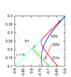
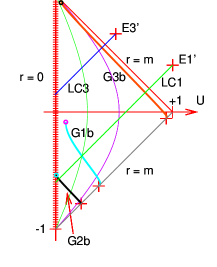
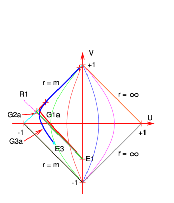
Fig. 4: Right panel: Three future-directed radial timelike geodesics emitted at points E1 and E3 in sector I of Fig. 3. The G1a has $\Gamma=1.1$, G2a has $\Gamma=3.0$ (i.e. larger energy in the Newtonian limit), G3a is ‘elliptic’ and has $\Gamma=0.5$. R1 is a radial ray emitted at E1; it hits the singularity at $r=0$ in a finite interval of the affine parameter. The crosses at the upper ends of G1a, G2a and G3a mark the first points on them at which $r<m$. Left panel: The continuation of G1a, G2a and G3a into sector II of Fig. 3. Their endpoints, marked with dots, are at the turning points. LC1 is the radial generator of the past light cone of E1^′ – the copy of E1 in sector I^′ of Fig. 3, LC3 is the analogue of LC1 for point E3^′. See the text for more explanation. Upper inset: An enlarged image of the area around the upper endpoints of G1a and G2a.

In choosing the initial point E3 of the elliptic geodesic G3a one must ensure that the initial $r=r_{i}$ is smaller than the $r_{{\rm TP}-}$ of (3.5) (otherwise, $\Gamma^{2}-E\phi<0$ at the initial point, and the numerical program will refuse to proceed). Consequently, $(t_{i},r_{i})$ are more convenient initial data than $(U_{i},V_{i})$. Given $m=0.95$, we thus choose

$$(t_{i},r_{i})=(0.1,\ \ r_{{\rm TP}-}-0.2).$$ (4.1)

Then we calculate the initial $\zeta$ from (2.2), the initial $(P,Q)$ from (2.6) and the initial $(U,V)$ from (2.7). From this point on, we follow the scheme described in the preceding paragraph: we send the ingoing radial timelike geodesic G3a towards the future, see the right panel of Fig. 4.

The left panel of Fig. 4 shows the continuation of the three geodesics into sector II, these are G1b, G2b and G3b, respectively (see below for a technical comment). Their upper endpoints are at their turning points. The line marked LC1 is the radial generator of the past light cone of E1^′, the copy of point E1 in sector I^′ of Fig. 3. The turning points of G1b and G2b lie to the future of LC1. This means that if they were continued beyond the turning points, they could not enter the causal past of E1^′, so they could not carry a message to the past of E1^′, i.e. causality is not broken in these two cases. The point E3^′ is the copy of E3 in sector I^′, the line LC3 is the radial generator of the past light cone of E3^′. One can see that also for this geodesic, the turning point lies to the future of LC3, so causality is not broken.

Here comes the technical comment: as stated earlier, G1a, G2a and G3a are tangent to the horizon the point of contact, so numerical approximation errors cause that G1b, G2b and G3b cannot get off the horizon on the other side. Therefore, the initial values of $V$ in sector II were corrected by $V\to V+10^{-6}$. This correction is invisible at the scale of Fig. 4. See Appendix E for more comments and technical details.

Figure 5 shows the two lower panels of Fig. 4 in their correct relative positions.

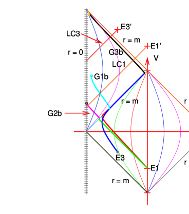
Fig. 5: The two lower panels of Fig. 4 put into their correct relative positions.

All three geodesics G1b, G2b and G3b have their turning points to the future of the past light cones of the copies of their points of origin, E1 and E3. It is thus clear that if they were continued beyond the turning points, they could not enter the causal past of E1^′ and E3^′, respectively, so could not carry messages from E1 and E3 to the past of E1^′ and E3^′. Consequently, the identifications of the asymptotically flat regions do not lead to causality breaches in these numerical examples. It remains an open problem to prove by a formal mathematical reasoning that this is so for all geodesics.

5. Nonradial timelike and null geodesics

The turning points of nonradial timelike or null geodesics are at the values of $r$ that obey $\Gamma^{2}-E\phi=0$ in (3.2) – (3.3), which is equivalent to

$$\Gamma^{2}r^{4}-\left(\varepsilon r^{2}+{J_{0}}^{2}\right)\left(r^{2}-2mr+m^{2}\right)=0$$ (5.1)

and also to

$$\left(\Gamma^{2}/E-1\right)r^{2}+2mr-m^{2}=0.$$ (5.2)

Equivalently, (5.2) may be written as

$$r=m\frac{1-\sigma|\Gamma|/\sqrt{E}}{1-\Gamma^{2}/E}\equiv\frac{m}{1+\sigma|\Gamma|/\sqrt{E}},\qquad\sigma=\pm 1.$$ (5.3)

This is still an equation to solve (because $E$ depends on $r$), but it it is more useful than (5.1) for a discussion. The fourth-degree equation (5.1) may have 0 to 4 real solutions for $r$. If it has any solutions, then those with $\sigma=+1$ have $r<m$, and those with $\sigma=-1$ either have no physical implications (because $r<0$ or $r\to\pm\infty$ when $|\Gamma|/\sqrt{E(r)}\geq 1$) or have $r>m$ (when $|\Gamma|/\sqrt{E(r)}<1$). The latter are irrelevant for the problem of causality because they do not enter the black hole region.

Equation (5.3) has elementary solutions for null geodesics, for which $\varepsilon=0$ and so $E={J_{0}}^{2}/r^{2}$. For $\sigma=+1$, the solution is

$${\overset{N}{r}}{}_{\rm TP}=\frac{1}{2}\ \left|J_{0}/\Gamma\right|\left(-1+\sqrt{1+4m\left|\Gamma/J_{0}\right|}\right)\equiv\frac{2m}{1+\sqrt{1+4m\left|\Gamma/J_{0}\right|}}<m$$ (5.4)

(the other solution with $\sigma=+1$ in (5.3) has minus in front of the square root in (5.4), so $r<0$ and such a TP does not exist). The solution (5.4) exists for all values of $m$, $\Gamma$ and $J_{0}$, and $\lim_{J_{0}\to 0}{\overset{N}{r}}{}_{\rm TP}=0$, which is consistent with our earlier finding that a radial null geodesic can hit $r=0$.

For $\sigma=-1$, two extra solutions of (5.3) (i.e. two additional TPs) exist when

$$4m|\Gamma/J_{0}|<1.$$ (5.5)

For these, ${\overset{N}{r}}{}_{\rm TP}>m$ as announced, but they create an interesting situation. They are

$$\left[\begin{array}[]{l}{\overset{N}{r}}{}_{\rm TP4}\\ \\ {\overset{N}{r}}{}_{\rm TP5}\end{array}\right]=\left[\begin{array}[]{l}{\displaystyle{\frac{2m}{1-\sqrt{1-4m\left|\Gamma/J_{0}\right|}}}}\\ \\ {\displaystyle{\frac{2m}{1+\sqrt{1-4m\left|\Gamma/J_{0}\right|}}}}\\ \end{array}\right].$$ (5.6)

Then, the set of of nonradial null geodesics splits into two families. In one, the geodesics (light rays) move between ${\overset{N}{r}}{}_{\rm TP}$ and ${\overset{N}{r}}{}_{\rm TP5}$, in the other they move between ${\overset{N}{r}}{}_{\rm TP4}$ and infinity. The geodesics of the second family never leave sector I, and so are irrelevant for the problem of causality. But the geodesics of the first family cross the horizon from sector I into sector II, and then continue to sector I^′. These are relevant, and they will be mentioned again in the next section.

When $4m|\Gamma/J_{0}|=1$, we have ${\overset{N}{r}}{}_{\rm TP5}={\overset{N}{r}}{}_{\rm TP4}\ {\overset{\rm def}{=}}\ {\overset{N}{r}}{}_{\rm TP}$. Then the geodesics of the two families mentioned above approach the TP from opposite sides and bounce – one towards infinity, the other towards the horizon. This situation is qualitatively not much different from that with $4m|\Gamma/J_{0}|<1$.

6. Numerical examples of nonradial geodesics

We now numerically calculate a nonradial timelike geodesic J1a and a nonradial null geodesic N1a that cross the horizon outside in, with the initial point in sector I. We take

$$\left(m,\Gamma,J_{0}\right)=(0.95,\quad 3.0,\quad 2.6);$$ (6.1)

the first parameter as in this whole paper, the second as for the radial geodesic G2a, the third one chosen at random, and we take the same E1 as before for the initial point with the coordinates $(U,V)=(0.0,-0.6)$. With $J_{0}\neq 0$ the geodesics do not stay in the initial $(U,V)$ plane, but go around the $V$ axis. For comparing them with the radial one, we rotate each of their points around the $r=0$ (i.e., $U=-1$) axis into the $(U,V)$ plane. (This happens simply by placing the $(U,V)$ coordinates of a point P in the $(U,V)$ plane and ignoring the fact that P has a nonzero $\varphi$. An illustration is given at the end of this section.) The comparison of those projections with the radial G2a is shown in Fig. 6. Both projections are close to G2a throughout sector I. While crossing the horizon, the projections of J1a and N1a are offset further than G2a, but reach the turning point also above the past light cone of E^′. The projection of N1a stays between that of J1a and G2a and, for better transparency, is not shown in sector I.

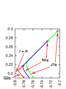
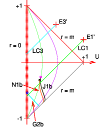
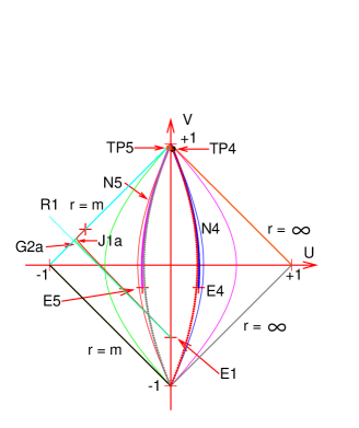
Fig. 6: Right panel: The radial geodesic G2a and the image of the nonradial timelike geodesic J1a going off point E1 in sector I of Fig. 3. At this scale they nearly coincide. The image of the nonradial null geodesic N1a is squeezed between them and invisible. The cross nearly on $r=m$ marks the endpoint of J1a (the first point at which $r<m$). The upper inset: A closeup view on the neighbourhood of the points where the geodesic G2a and the images of N1a and J1a cross the horizon. The crosses that seemingly lie on $r=m$ mark the first points on the geodesics at which $r<m$. Left panel: The continuation of G2a and of the images of N1a and J1a into sector II of Fig. 3. The turning points of the nonradial geodesics are above the past light cone of E1^′. See the text for explanations concerning the other curves and points in the right panel.

For illustration, the lower right panel of Fig. 6 shows also two nonradial null geodesics N4 (initially ingoing) and N5 (initially outgoing), whose parameters obey (5.5):

$$\left(m,\Gamma,J_{0}\right)=(0.95,\quad 3.0,\quad 11.41).$$ (6.2)

They are examples of the nonradial null geodesics with large $|J_{0}|$, discussed in connection with (5.5) and (5.6). The $r$ coordinates of their extra turning points are

$$\left({\overset{N}{r}}{}_{\rm TP5},{\overset{N}{r}}{}_{\rm TP4}\right)=(1.8453688474864800,\quad 1.9579644858468537).$$ (6.3)

The dotted arcs are at $r={\overset{N}{r}}{}_{\rm TP5}$ (the left one) and $r={\overset{N}{r}}{}_{\rm TP4}$ (the right one). The initial point E4 of N4 has coordinates

$$(t,r)=(-0.2,\quad{\overset{N}{r}}{}_{\rm TP4}+0.005).$$ (6.4)

The N4 goes towards smaller $r$ until it reaches the turning point TP4. Then it becomes outgoing and recedes to infinity. The $(U,V)$ coordinates of TP4 are

$$(U,V)_{\rm TP4}=(0.016897625562350471,\quad 0.95928250934355219).$$ (6.5)

The other geodesic, N5, goes off point E5, with coordinates

$$(t,r)=(-0.2,\quad{\overset{N}{r}}{}_{\rm TP5}-0.005).$$ (6.6)

and is initially outgoing. It reaches the turning point TP5 at $r={\overset{N}{r}}{}_{\rm TP5}$, where it becomes ingoing. The $(U,V)$ coordinates of TP5 are

$$(U,V)_{\rm TP5}=(-0.012965471226367431,\quad 0.96888417351466494).$$ (6.7)

Unfortunately, N5 crosses the horizon so near to $(U,V)=(0,1)$ that its continuation into sector II could not be calculated even at double precision in Fortran 90.

Another null geodesic, with the same parameters as N5 and the same initial point E5 but ingoing from the start, coincided with N5 at the scale of Fig. 6 and had the point of contact with the horizon also very near to $(U,V)=(0,1)$.

As a curiosity, Fig. 7 shows the view on geodesics J1a, J1b, N1a and N1b from atop the $r=0$ axis in Fig. 5. The radial coordinate here is $(U+1)$ with $U$ as in Fig. 5, the origin is at $U=-1$, the $V$ axis goes perpendicularly to the figure plane towards the viewer, and

$$X=(U+1)\cos\varphi-1,\qquad Y=(U+1)\sin\varphi.$$ (6.8)

The initial point (the right end of J1a and N1a) is at $(U,\varphi)=(0,0)$. The consecutive values of $\varphi$ were calculated using (3.4). The short horizontal bars are where the geodesics cross the horizon. The inclined straight segment and the arc at its end show how the projections of the points of the geodesics to the plane of Fig. 6 were constructed. The projections of J1a and N1a nearly coincide between $X=0$ and $X=-0.78$.

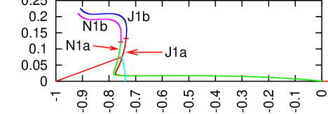
Fig. 7: The view on nonradial geodesics from atop the $r=0$ axis in Fig. 5. See the text for explanation.

Finally, Fig. 8 shows the view on J1a and J1b analogous to that in Fig. 7, but in the $(x,y)=(r\cos\varphi,r\sin\varphi)$ coordinates. In this projection, N1a and N1b nearly coincide with J1a and J1b, so they are not shown. As can be seen, in these coordinates the geodesic is not tangent to the horizon. This agrees with (3.2), which shows that ${{\rm d}{r}}/{{\rm d}{s}}=\pm\Gamma\neq 0$ at $r=m$. Drawing Fig. 8 required a trick that is explained in Appendix F.

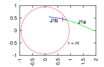
Fig. 8: The view on the geodesics J1a and J1b analogous to Fig. 7, but in the $(x,y)=(r\cos\varphi,r\sin\varphi)$ coordinates. See the text for a comment.

7. Summary and conclusions

The aim of this paper was to verify whether an observer in the maximally extended extreme RN spacetime with asymptotically flat regions (AFRs) identified can send messages to its own past by means of timelike or null geodesics (in other words, whether the identifications of the AFRs lead to acausality). By this opportunity, images of geodesics in this extension were derived and discussed.

In Sec. 2., the maximal extension of the extreme RN metric was re-derived in more detail than in standard textbook presentations. In particular, in the coordinates of the extension chosen here, the shapes of the singular set $r=0$ and of the lines of constant $t$ and $r$ were explicitly calculated.

In Sec. 3., the geodesic equations in the extreme RN metric were discussed. It was shown that radial null geodesics (NGs) can hit the singularity at $r=0$, and those that do stop there. Timelike and nonradial NGs that cross the horizon $r=m$ are tangent to it in the $(U,V)$ coordinates of the maximal extension. The $r$-coordinate of the turning point (TP) of a radial timelike geodesic (TG) is given by the simple Eq. (3.5).

In Sec. 4., three examples of radial TGs were numerically calculated, with different values of the energy constant $\Gamma$. As predicted, they cross the horizon tangentially. Their TPs lie to the future of the past light cones (PLCs) of the copies of their initial points (the copies are created by identifying the asymptotically flat regions). Therefore, they cannot carry messages to the past of their emitters, i.e. the identifications of the AFRs do not lead to causality breaches.

In Sec. 5., general properties of nonradial TGs and NGs were discussed. For NGs, the $r$-coordinates of their TPs are given by explicit exact formulae, and so they were discussed in more detail. One TP exists for every nonradial NG and lies inside the horizon. With sufficiently large $|J_{0}|$ (where $J_{0}$ is the angular momentum constant), two extra TPs exist outside the horizon. In this case, the nonradial NGs move either between the outermost TP and the infinity, or between the other two TPs. In the second case, they cross the horizon and go into the next AFR.

In Sec. 6., numerical examples of the nonradial geodesics that cross the horizon were presented, one timelike (named J1) and one null (named N1). For them, too, the TPs lie to the future of the PLCs of the copies of their emission points, so causality is not broken. Two numerical examples of nonradial NGs with large $|J_{0}|$ that illustrate the calculations of Sec. 5. were also presented. In addition, the projections of J1 and N1 on surfaces of constant $V$, one in the $(U,\varphi)$ coordinates and one in the $(r,\varphi)$ coordinates, were shown in illustrations.

In contrast to the RN metric with $e^{2}<m^{2}$, in the $e^{2}=m^{2}$ case all numerical examples show the same:

Let E be the initial point of a geodesic in the asymptotically flat region I of the maximally extended extreme RN spacetime. Let E^′ be the copy of E in the first future copy of I. A timelike or nonradial null geodesic emitted at E will have its turning point outside the past light cone of E^′. Thus, a message sent by this geodesic will not reach the causal past of E^′. This means that the identification of E^′ with E does not cause acausality.

However, it remains an open problem to prove the same by a formal mathematical reasoning. Nonexistence (here: of geodesics breaking causality) cannot be proved by examples alone.

Appendix A The singularity of (2.1) at $r=m$ is spurious

The orthonormal tetrad of differential forms connected with the metric (2.1) is

$$e^{0}=(1-m/r){\rm d}t,\quad e^{1}=(1-m/r)^{-1}{\rm d}r,\quad e^{2}=r{\rm d}\vartheta,\quad e^{3}=r\sin\vartheta{\rm d}\varphi.$$ (A1)

The independent nonzero tetrad components of the Riemann tensor in this tetrad are

$$R_{0101} = 2m/r^{3}-3m^{2}/r^{4},\qquad R_{2323}=-2m/r^{3}+m^{2}/r^{4}$$

$$R_{0202} = R_{0303}=-R_{1212}=-R_{1313}=-\frac{m}{r^{3}}\left(1-\frac{m}{r}\right).$$ (A2)

They are all regular at $r=m$, so there is no curvature singularity at this $r$. $\square$

Appendix B Solving (2.2) numerically for $r$ given $\zeta(r)$

While numerically integrating the geodesic equations, we are confronted with the problem of determining $r$ from (2.2) for a given $\zeta$. This is done by the bisection method, separately in the $r\in(0,m)$ and in the $r\in(m,\infty)$ domain. In $(0,m)$, the initial bounds for $r$ are obviously $0<r<m$. In $(m,\infty)$, the lower bound is $r=m$, but the upper bound is not self-evident. This is how it can be determined.

Since the function $\zeta(r)$ changes monotonically in the whole $(-\infty,+\infty)$ range, we have to find a function $Z(r)$ that has the same range, $Z(r)<\zeta(r)$ for all $r\in(m,\infty)$ and $Z(r_{1})=Z_{1}$ is easy to solve for $r_{1}$ given $Z_{1}$. For every $x>0$ we have $2\ln x>-1/x$ (the proof is left as an exercise for the reader). Hence, for $r>m$ we have in (2.2)

$$2m\ln|r/m-1|>-m/(r/m-1)\equiv-m^{2}/(r-m)\quad{\rm for\ all}\ \ r>m.$$ (B1)

Consequently,

$$\zeta(r)>Z(r)\ {\overset{\rm def}{=}}\ r-m-2m^{2}/(r-m)\quad{\rm for\ all}\ \ r>m.$$ (B2)

Thus, given $\zeta_{0}\ {\overset{\rm def}{=}}\ \zeta(r_{0})$, where $r_{0}$ is to be found, we solve $Z(r_{1})=\zeta_{0}$ for $r_{1}$ and find

$$r_{1}=m+\frac{1}{2}\ \left(\zeta_{0}+\sqrt{{\zeta_{0}}^{2}+8m^{2}}\right)$$ (B3)

(the other solution, with “$-$” in front of $\sqrt{\ }$, would have $r_{1}<m$). By construction, $r_{0}<r_{1}$. This calculation is illustrated in Fig. 9.

Fig. 9: Comparison of the functions $\zeta(r)$ and $Z(r)$ for small $r>m$ (left panel) and for large $r$ (right panel). The right panel shows how to determine the initial $r_{1}$ in finding $r_{0}$ for a given $\zeta(r_{0})$.

Appendix C Christoffel symbols in the $(t,\zeta)$ coordinates

The symbol $S_{1}$ stands for

$$S_{1}=1-m/r,$$ (C1)

so $S_{1}=0$ at $r=m$. The formulae below show that there is no singularity in the Christoffel symbols there (in the coordinates of (2.1), some Christoffel symbols contain the factor $S^{-1}$). Only the independent nonzero components of $\begin{Bmatrix}\alpha\ \\ \beta\gamma\end{Bmatrix}$ are shown; $(x^{0},x^{1},x^{2},x^{3})=(t,\zeta,\vartheta,\varphi)$.

$$\mbox{\small$\begin{Bmatrix}0\ \\ 01\end{Bmatrix}$}=\mbox{\small$\begin{Bmatrix}1\ \\ 00\end{Bmatrix}$}=\mbox{\small$\begin{Bmatrix}1\ \\ 11\end{Bmatrix}$}=mr^{-2}{S_{1}},$$ (C2)

$$\mbox{\small$\begin{Bmatrix}1\ \\ 22\end{Bmatrix}$}=\mbox{\small$\begin{Bmatrix}1\ \\ 33\end{Bmatrix}$}/{\sin}^{2}(\vartheta)=-r,$$ (C3)

$$\mbox{\small$\begin{Bmatrix}2\ \\ 12\end{Bmatrix}$}=\mbox{\small$\begin{Bmatrix}3\ \\ 13\end{Bmatrix}$}=r^{-1}{S_{1}}^{2},$$ (C4)

$$\mbox{\small$\begin{Bmatrix}2\ \\ 33\end{Bmatrix}$}=-\cos(\vartheta)\sin(\vartheta),\qquad\mbox{\small$\begin{Bmatrix}3\ \\ 23\end{Bmatrix}$}=\cos(\vartheta)/\sin(\vartheta).$$ (C5)

Appendix D The limit of ${{\rm d}{V}}/{{\rm d}{U}}$ at $r\to m$ with $\sigma=-1$ and $\Gamma>0$

Since $P=1$ and $\phi=0$ at $r=m$, we have in (3.11)

$$\lim_{r\to m}\frac{1-P^{2}}{\phi}=\lim_{r\to m}\left[\frac{-2P{{\rm d}{P}}/{{\rm d}{s}}}{2(1-m/r)(m/r^{2}){{\rm d}{r}}/{{\rm d}{s}}}\right].$$ (D1)

Using (3.2) with ${{\rm d}{r}}/{{\rm d}{s}}<0$ and (3.9) with $\sigma=-1$, we obtain from this

$$\lim_{r\to m}\frac{1-P^{2}}{\phi}=\lim_{r\to m}\left[\frac{P\left(\Gamma+\sqrt{\Gamma^{2}-E\phi}\right)}{(1-m/r)(m/r^{2})\sqrt{\Gamma^{2}-E\phi}}\times\frac{1-P^{2}}{\phi}\right].$$ (D2)

Hence,

$$\lim_{r\to m}\left\{\frac{1-P^{2}}{\phi}\left[1-\frac{r^{2}P}{m(1-m/r)}\ \left(\frac{\Gamma}{\sqrt{\Gamma^{2}-E\phi}}+1\right)\right]\right\}=0.$$ (D3)

But the second term in square brackets clearly tends to $(\mp\infty)$ as $r\to m^{\pm}$. So, (D3) can hold only when

$$\lim_{r\to m}\frac{1-P^{2}}{\phi}=0.\qquad\square$$ (D4)

Appendix E Crossing the horizon with numerical integration of the geodesic equations

As already stated in Sec. 4., the G1a, G2a and G3a curves in Fig. 4 approach the horizon tangentially. When their points of contact with $r=m$ were used as the initial points of their continuations into sector II, numerical imprecisions caused that the continuations kept going along $r=m$. The initial coordinates of the continuations had to be hand-corrected to manageable values. Here we demonstrate the consequences of this correction for the G3a,b geodesic, see Fig. 10.

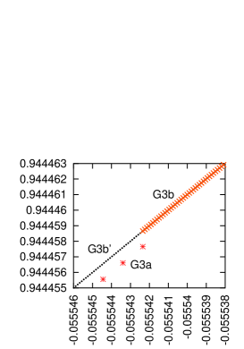
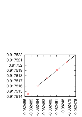
Fig. 10: Left panel: The neighbourhood of the upper endpoint of G3a. The artificially introduced jump $\Delta V=10^{-6}$ in the $V$ coordinate between the endpoint of G3a and the initial point of G3b is visible. The G3b^′ is the result of backtracking G3b from its upper end in Fig. 4 to the intersection with $r=m$. Right panel: The neighbourhood of the lower endpoint of G3b^′, where it crosses $r=m$. Here, the $V$ coordinates of points on G3b^′ (drawn with dots) coincide with those on G3a (drawn with crosses) to better than $10^{-6}$.

Recall: the G3a was numerically integrated from point E3 to the first point (call it P) at which $r$ became smaller than $m$. The $V_{P}$ coordinate of P was increased ‘by hand’ to $V^{\prime}_{P}=V_{P}+10^{-6}$. Then, the $(U_{P},V^{\prime}_{P})$ coordinates of P in sector I were transformed to $(\widetilde{U},\widetilde{V})=(1+U_{P},V^{\prime}_{P}-1)$ – the coordinates of the same point in sector II. Using $(\widetilde{U},\widetilde{V})$ as the initial data, the geodesic equations were integrated up to the turning point, at which $r=r_{{\rm TP}+}$ given by (3.5); this second segment of G3a is denoted G3b. The $(U,V)$ coordinates of the turning point were

$$(U_{f},V_{f})=(0.043718751055178640,\quad 0.93765063538654081).$$ (E1)

To verify the precision of the code, a past-directed radial timelike geodesic G3b^′ was sent from $(U_{f},V_{f})$ backward with the same $\Gamma$ (backward means towards increasing $r$, i.e. with $\sigma=+1$ in (3.9) – (3.10)). The endpoint of G3b^′ was where $r$ became larger than $m$. Figure 10 shows the relations between G3a, G3b and G3b^′ in the neighbourhood of point P. The left panel shows that at P G3b^′ coincides with G3b to better than $10^{-6}$; it also shows the jump between G3a and G3b. The right panel shows that at its lower end G3b^′ coincides with G3a to better than $10^{-6}$.

Appendix F Drawing Fig. 8

The hand-correction described at the beginning of Appendix E caused a visible jump in $r$. The geodesic J1b had its initial point in Fig. 8 at the short vertical bar. To close the gap, another geodesic J1b^′ was issued from the future endpoint of J1b backward, and allowed to cross the $r=m$ circle. This is the arc marked J1b in Fig. 8; it coincides with the proper J1b between the bar and the left endpoint.

In the first calculation it was assumed that the first value of $\varphi$ on J1b is the same as the last value on J1a, which caused another (small) discontinuity between J1a and J1b. Consequently, to make J1a and J1b^′ meet with the precision of $\Delta y=10^{-5}$ shown in the figure, the correction $\Delta\varphi=0.011826$ had to be applied to the value of $\varphi$ at the left end of J1b^′. It was determined by trial and error. The value of $\varphi$ does not appear in (3.1) – (3.3), so such manipulations with it did not require any change in the numerical algorithm of calculating the geodesics.

Acknowledgement. For some calculations, the computer algebra system Ortocartan [10, 11] was used.

References

- [1] A. Krasiński, Causality in the maximally extended Reissner–Nordström spacetime with identifications. Rep. Math. Phys., in press; arXiv 2409.03786.
- [2] H. Reissner, Über die Eigengravitation des elektrischen Feldes nach der Einsteinschen Theorie [On the self-gravitation of the electric field according to Einstein’s theory], Ann. Physik 50, 106 (1916).
- [3] G. Nordström, On the energy of the gravitational field in Einstein’s theory, Koninklijke Nederlandsche Akademie van Wetenschappen Proceedings 20, 1238 (1918).
- [4] B. Carter, The complete analytic extension of the Reissner–Nordström metric in the special case , Phys. Lett. 21, 423 (1966).
- [5] J. Plebański and A. Krasiński, An Introduction to General Relativity and Cosmology, second edition. Cambridge University Press 2024.
- [6] G. Lemaître, L’Univers en expansion [The expanding Universe], Ann. Soc. Sci. Bruxelles A53, 51 (1933); English translation: Gen. Relativ. Gravit. 29, 641 (1997), with an editorial note by A. Krasiński, Gen. Relativ. Gravit. 29, 637 (1997).
- [7] I. D. Novikov, R- i T-oblasti v prostranstve-vremeni so sfericheski-simetrichnym prostranstvom [R- and T-regions in a spacetime with a spherically symmetric space], Soobshcheniya GAISh 132, 3 (1964); English translation: Gen. Relativ. Gravit. 33, 2259 (2001), with an editorial note by A. Krasiński, Gen. Relativ. Gravit. 33, 2255 (2001). See also Ref. [8], pp. 397 – 438.
- [8] A. Krasiński, G. F. R. Ellis and M. A. H. MacCallum, Golden Oldies in General Relativity, Hidden Gems. Springer Verlag, Berlin Heidelberg (2013).
- [9] B. Carter, Black hole equilibrium states. Part I: Analytic and geometric properties of the Kerr solutions. In: Black Holes – les astres occlus. Edited by C. de Witt and B. S. de Witt. Gordon and Breach, New York, London, Paris 1973, p. 61. Reprinted in Gen. Relativ. Gravit. 41, 2874 (2009), with an editorial note by N. Kamran and A. Krasiński, Gen. Relativ. Gravit. 41, 2867 (2009).
- [10] A. Krasiński, The newest release of the Ortocartan set of programs for algebraic calculations in relativity. Gen. Relativ. Gravit. 33, 145 (2001).
- [11] A. Krasiński, M. Perkowski, The system ORTOCARTAN – user’s manual. Fifth edition, Warsaw 2000.