Phase diagram of the interacting partially directed self-avoiding walk attracted by a vertical wall

Abstract.

In the present paper, we consider the interacting partially-directed self-avoiding walk (IPDSAW) attracted by a vertical wall. The IPDSAW was introduced by Zwanzig and Lauritzen (J. Chem. Phys., 1968) as a manner of investigating the collapse transition of a homopolymer dipped in a repulsive solvent. We prove in particular that a surface transition occurs inside the collapsed phase between (i) a regime where the attractive vertical wall does not influence the geometry of the polymer and (ii) a regime where the polymer is partially attached at the wall on a length that is comparable to its horizontal extension, modifying its asymptotic Wulff shape. The latter rigorously confirms the conjecture exposed by physicists in (Physica A: Stat. Mech. & App., 2002). We push the analysis even further by providing sharp asymptotics of the partition function inside the collapsed phase.

Notation

Let $(a_{L})_{L\geq 1}$ and $(b_{L})_{L\geq 1}$ be two sequences of positive numbers. We will write

$$a_{L}\underset{L\to\infty}{\sim}b_{L}\quad\text{if}\quad\lim_{L\to\infty}a_{L}/b_{L}=1.$$ (0.1)

We will also write $({\rm{cst.}})$ to denote generic positive constants whose value may change from line to line. We denote by $\mathbb{N}=\{1,2,3,\ldots\}$ the set of positive integers while $\mathbb{N}_{0}=\{0,1,2,\ldots\}$ is the set of non-negative integers. If $X=(X_{i})_{i\in\mathbb{N}}$ is a random process, we note $X_{I}=(X_{i})_{i\in I}$ for every $I\subseteq\mathbb{N}$ and abbreviate $\{X_{I}>0\}:=\{X_{i}>0,\ i\in I\}$.

1. Introduction

The collapse transition of a polymer dipped in a repulsive solvent is a physical phenomenon that has been extensively studied in the physics literature (see e.g. [4, 6] for theoretical background and more recently [16] or [9, Section 8] for computational background). There are so far very few mathematical models for which the collapse transition has been rigorously proven. Among this latter class of models, the Interacting Partially Directed Self-Avoiding Walk (IPDSAW) was initially introduced in [19] and investigated first with the help of combinatorial tools (see e.g. [8, 15]) and then, in the last decade, thanks to a random walk representation of the trajectories. This probabilistic perspective allowed for a much deeper mathematical understanding of both the phase transition and the geometric features of a typical trajectory sampled from the polymer measure, in each regime (see [2] for a review).

Physicists have also considered the effect of an interaction between the polymer and the container inside which the poor solvent is kept, see e.g. [13, 17]. Such an additional interaction with the bottom of the container triggers a surface transition inside the collapsed phase of the IPDSAW, which was recently put on rigorous grounds in [12]. In the present paper, we focus on another interaction of interest, that is an attractive interaction between the polymer and one of the vertical walls of the container. In particular, we display the phase diagram of the model and exhibit another surface transition inside the collapsed phase.

When only the solvent-monomers interactions are taken into account, it was shown in [11] that, inside the collapsed phase, a typical configuration of the polymer is made of a macroscopic volume called bead, which is unique since only finitely many monomers are to be found outside this bead. For a polymer of length $L\in\mathbb{N}$, this bead, once rescaled horizontally and vertically by $\sqrt{L}$ converges in probability towards a deterministic Wulff shape (see [1]). In [12], the polymer is investigated inside its collapsed phase and some additional interactions are taken into account between the monomers and the bottom of the container. In order to keep the model tractable, a geometric restriction has been imposed on the allowed configurations, namely they are required to describe a unique bead. In the present paper, although we consider additional interactions as well (this time between the monomers and the vertical walls), we managed to get rid of the single bead restriction and display our result in the general framework. From that perspective, the results displayed here are more ambitious.

1.1. The IPDSAW with an attractive wall

The configurations of the polymer are modeled by random walk paths on $\mathbb{Z}^{2}$ that are self-avoiding and take exclusively unitary steps upwards, downwards and to the right (see Fig. 1). The fact that the polymer is placed in a repulsive solvent is taken into account by assuming that the monomers try to exclude the solvent and therefore attract one another. For this reason, any pair of non-consecutive vertices of the walk that are adjacent on the lattice is called self-touching and the interactions between monomers are taken into account by assigning an energetic reward $\beta$ to the polymer for each self-touching. In the present paper, we take into account another interaction between the polymer and the medium around it, namely an attraction of the monomer at the vertical wall of the container. This interaction is of intensity $\delta$. Note that we consider non-negative interactions, i.e. $(\beta,\delta)\in\mathcal{Q}:=[0,+\infty)^{2}$. It is convenient to represent the configurations of the model as collections of oriented vertical stretches separated by horizontal steps. To be more specific, for a polymer made of $L\in\mathbb{N}$ monomers, the set of allowed paths is $\Omega_{L}:=\bigcup_{N=1}^{L}\mathcal{L}_{N,L}$, where $\mathcal{L}_{N,L}$ consists of all the collections made of $N$ vertical stretches that have a total length $L-N$, that is

$$\textstyle\mathcal{L}_{N,L}=\Bigl{\{}\ell:=(\ell_{i})_{i=1}^{N}\in\mathbb{Z}^{N}:\sum_{n=1}^{N}|\ell_{n}|+N=L\Bigr{\}}.$$ (1.1)

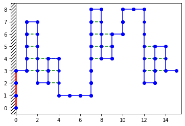
Figure 1. Picture of the trajectory $\ell\in\mathcal{L}_{15,54}$ whose vertical stretches are $(3,4,-5,2,-3,0,0,7,-4,2,2,0,-6,3,-2)$. The wall interaction is highlighted in red, and the self-interaction is represented by a dashed line.

With this representation, the modulus of a given stretch corresponds to the number of monomers constituting this stretch (and the sign gives the direction upwards or downwards). For convenience, we require every configuration to end with a horizontal step, and we note that any two consecutive vertical stretches are separated by a horizontal step. The latter explains why $\sum_{n=1}^{N}|\ell_{n}|$ must equal $L-N$ in order for $\ell=(\ell_{i})_{i=1}^{N}$ to be associated with a polymer made of $L$ monomers (see Fig. 1). We define the set of all trajectories as $\Omega=\cup_{L\geq 1}\Omega_{L}$ and for a given trajectory $\ell\in\Omega$, we let $N_{\ell}$ be its horizontal extension (that is also its number of vertical stretches) and $|\ell|$ be its total length, i.e., $\ell\in{\mathcal{L}}_{N_{\ell},|\ell|}$. The interactions between the polymer and the medium around it are taken into account in a Hamiltonian associated with each path $\ell\in\Omega_{L}$ and denoted by $\textstyle H_{L,\beta,\delta}(\ell)$. To be more specific, for every configuration $\ell\in\Omega_{L}$, the attraction between the vertical hard wall and the polymer holds along the first vertical stretch of the configuration as $\delta|\ell_{1}|$. Moreover, the repulsion between the monomers and the solvent is taken into account by rewarding energetically those pairs of consecutive stretches with opposite directions, i.e.,

$$\textstyle H_{L,\beta,\delta}(\ell_{1},\ldots,\ell_{N})=\delta|\ell_{1}|+\beta\sum_{n=1}^{N-1}(\ell_{n}\;\widetilde{\wedge}\;\ell_{n+1}),$$ (1.2)

where

$$x\,\widetilde{\wedge}\,y=\begin{dcases*}|x|\wedge|y|&if $xy<0$,\\ 0&otherwise.\end{dcases*}$$ (1.3)

With the Hamiltonian in hand we can define the polymer measure as

$$P_{L,\beta,\delta}(\ell)=\frac{e^{H_{L,\beta,\delta}(\ell)}}{Z_{L,\beta,\delta}},\quad\ell\in\Omega_{L},$$ (1.4)

where $Z_{L,\beta,\delta}$ is the partition function of the model, i.e.,

$$Z_{L,\beta,\delta}=\sum_{N=1}^{L}\sum_{\ell\in\mathcal{L}_{N,L}}\,e^{H_{L,\beta,\delta}(\ell)}.$$ (1.5)

1.2. Reminder on the model without a wall

The particular case where the interaction between the monomers and the vertical wall is switched off (corresponding to $\delta=0$) has been studied in depth in [1, 11, 14]. In this case the existence of the exponential growth rate of the partition function sequence $(Z_{L,\beta,0})_{L\geq 1}$ is obtained by subadditivity (in $L$) of the logarithm of the former sequence combined with Fekete’s lemma. Then, the free energy defined as

$$f(\beta,0)=\lim_{L\to\infty}\frac{1}{L}\log Z_{L,\beta,0},$$ (1.6)

allows us to divide the phase diagram into (i) an extended phase $[0,\beta_{c})=\{\beta\geq 0\colon f(\beta,0)>\beta\}$ and (ii) a collapsed phase $[\beta_{c},\infty)=\{\beta\geq 0\colon f(\beta,0)=\beta\}$. Note that the inequality $f(\beta,0)\geq\beta$ is easily obtained with the following observation. For $L\in\{k^{2}\colon k\in\mathbb{N}\}$, we restrict the partition function to a single trajectory $\widetilde{\ell}\in{\mathcal{L}}_{\sqrt{L},L}$ defined as

$$\widetilde{\ell}_{i}:=(-1)^{i-1}(\sqrt{L}-1)\quad\text{ for}\quad i\in\{1,\dots,\sqrt{L}\}.$$ (1.7)

Thus, the Hamiltonian of $\widetilde{\ell}$ at $\delta=0$ equals $\beta(\sqrt{L}-1)^{2}=\beta L(1+o_{L}(1))$ which guarantees us that $f(\beta,0)\geq\beta$.

1.3. Outline of the paper

In Section 2, we state and comment the most important results of the present paper. To begin with, we describe the three different phases (extended, collapsed and glued) into which the phase diagram is divided. Then, we present the surface transition that splits the collapsed phase into three regimes (desorbed-collapsed, critical and adsorbed-collapsed). We provide the formula of the associated critical curve and we display some sharp asymptotics of the partition function in each regime. In Section 3, the phase transitions are proven rigorously, namely the existence of critical curves separating the three aforementioned phases. We take this opportunity to introduce the random walk representation that allows us to provide an alternative expression of the partition function using a random walk of law $\mathbf{P}_{\beta}$ (defined in (2.9)). In Section 4 we introduce notation and auxiliary mathematical tools that are required to prove our main results. Thus, in Section 4.1, we settle a class of auxiliary partition functions involving a random walk of law $\mathbf{P}_{\beta}$ constrained to enclose an atypically large area. Some sharp asymptotics of those partition functions are provided in Section 4.5 and proven in Section 6. In section 4.2 we display a method to decompose each polymer trajectory into beads that consist of collections of non-zero vertical stretches whose signs alternate. Such decomposition is useful when working inside the collapsed phase because a typical trajectory sampled from the polymer measure turns out to be made of a unique macroscopic bead. Sections 4.3 and 4.4 are dedicated to two tilted versions of the law of a random walk under $\mathbf{P}_{\beta}$. One tilting is homogeneous in time whereas the other one is inhomogeneous. Both versions will be applied to study random walk trajectories enclosing an abnormally large area. Some local limit theorems are stated in Section 4.6 concerning both the arithmetic area and the final position of a random walk sampled from the (above mentioned) inhomogeneous tilting of $\mathbf{P}_{\beta}$. Finally, some bounds on the polymer horizontal extension inside the collapsed phase are displayed in Section 4.7. With Section 5, we prove the existence of the surface transition and compute its critical curve. Finally, with Sections 6 and 7 we prove the asymptotics of the partition function corresponding to each of the three regimes in the collapsed phase.

2. Results

We distinguish between two types of results. First, in Section 2.1 below, we describe the phase diagram of the model which is divided into three phases: extended, collapsed and glued (denoted respectively by ${\mathcal{E}}$, ${\mathcal{C}}$ and ${\mathcal{G}}$). A typical trajectory sampled from $P_{L,\beta,\delta}$ has a horizontal extension of order $L$ inside ${\mathcal{E}}$, $o(L)$ inside ${\mathcal{C}}$, and finally, inside ${\mathcal{G}}$, such trajectory takes only finitely many horizontal steps after a very long vertical stretch attached to the wall. The second type of results consists in analyzing more in depth the collapsed phase. The free energy in ${\mathcal{C}}$ is equal to $\beta$, which guarantees us that there is no phase transition inside ${\mathcal{C}}$. However, depending on the value of $(\beta,\delta)\in{\mathcal{C}}$ we will observe that the behavior of the polymer with respect to the attractive wall may change drastically. This latter phenomenon is associated with a surface transition taking place along a critical curve that divides ${\mathcal{C}}$ into three regimes:

• A desorbed-collapsed (${\mathcal{D}}{\mathcal{C}}$) regime inside which $\delta$ is not large enough to pin the first vertical stretch of the polymer to the wall. Thus, the first vertical stretch remains of length $O(1)$;

• An adsorbed-collapsed (${\mathcal{A}}{\mathcal{C}}$) regime inside which $\delta$ is large enough for the polymer to be pinned at the attractive wall along its first vertical stretch, on a length $O(\sqrt{L})$;

• A critical regime at which the first vertical stretch has length $O(L^{1/4})$.

2.1. Phase transition

Let us denote by $f(\beta,\delta)$ the free energy of the system, that is the exponential growth rate of $(Z_{L,\beta,\delta})_{L\geq 1}$. It turns out that $f(\beta,\delta)$ may actually be expressed as the maximum of $\delta$ and $f(\beta,0)$. We recall that $f(\beta,0)\geq\beta$ by (1.7) and that $\mathcal{Q}:=[0,+\infty)^{2}$.

Proposition 2.1.

For every $(\beta,\delta)\in\mathcal{Q}$, the following limit exists:

$$\underset{L\longrightarrow\infty}{\lim}\frac{1}{L}\log Z_{L,\beta,\delta}=f(\beta,\delta)\in[0,\infty),$$ (2.1)

and $f(\beta,\delta)=f(\beta,0)\vee\delta$.

The free energy allows us to distinguish between three phases: collapsed (${\mathcal{C}}$), extended (${\mathcal{E}}$) and glued along the vertical wall (${\mathcal{G}}$). We let $\beta_{c}$ be the unique positive solution to the equation $\Gamma_{\beta}=1$ with

$$\Gamma_{\beta}=c_{\beta}\,e^{-\beta}=\frac{e^{-\beta}+e^{-3\beta/2}}{1-e^{-\beta/2}}$$ (2.2)

with $c_{\beta}$ properly defined in (2.9).

Definition 2.2.

Rigorously, the three phases are

• ${\mathcal{E}}:=\{(\beta,\delta)\in\mathcal{Q}\colon\,\beta<\beta_{c}{\rm\ and\ }f(\beta,\delta)>\delta\}$

• ${\mathcal{C}}:=\{(\beta,\delta)\in\mathcal{Q}\colon\,\beta\geq\beta_{c}{\rm\ and\ }f(\beta,\delta)=\beta\}$

• ${\mathcal{G}}:=\{(\beta,\delta)\in\mathcal{Q}\colon\,f(\beta,\delta)=\delta\}$

With Proposition 2.1, we may rewrite these three phases as follows:

$${\mathcal{E}} :=\{(\beta,\delta)\in\mathcal{Q}\colon\,\beta<\beta_{c},\ \delta\leq f(\beta,0)\},$$

$${\mathcal{C}} :=\{(\beta,\delta)\in\mathcal{Q}\colon\,\beta\geq\beta_{c},\ \delta\leq\beta\},$$

$${\mathcal{G}} :=\{(\beta,\delta)\in\mathcal{Q}\colon\,\delta>f(\beta,0)\}.$$

Fig. 2 provides a picture of the phase diagram. We observe that the boundaries meet at the tri-critical point $(\beta_{c},\beta_{c})$.

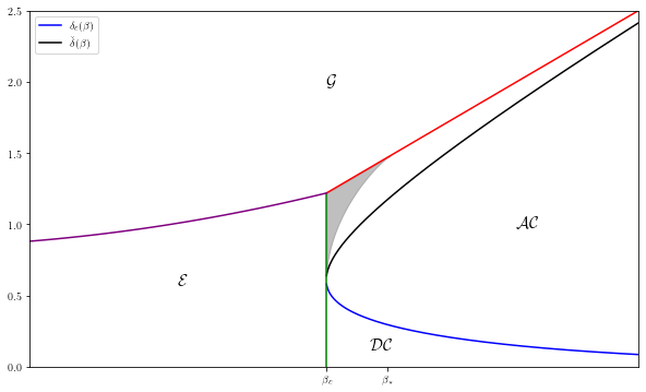
Figure 2. Phase diagram of the polymer pinned at the vertical wall. The three phases ${\mathcal{E}}$, ${\mathcal{C}}$ and ${\mathcal{G}}$ are separated by the purple ($\delta=f(\beta,0)$), red ($\delta=\beta$) and green ($\beta=\beta_{c}$) curves. The surface transition between the regimes ${\mathcal{D}}{\mathcal{C}}$ and ${\mathcal{A}}{\mathcal{C}}$ is indicated by the blue curve ($\delta=\delta_{c}(\beta)$), for which we have an explicit expression. A change of convexity happens for the Wulff shape at the black curve ($\delta=\check{\delta}(\beta)$). The bounded grey set ${\mathcal{C}}_{\rm bad}$, see (2.17), is where our method fails and has been computed numerically. The first coordinate of the rightmost point in ${\mathcal{C}}_{\rm bad}$, denoted by $\beta_{*}$, is smaller than $\pi/\sqrt{3}\approx 1.81$ (rigorously) and around 1.47 (numerically).

The phase transitions being now identified, the rest of the present section is dedicated to the collapsed phase ${\mathcal{C}}$ and in particular to the surface transition that takes place inside ${\mathcal{C}}$.

2.2. Surface transition

Figuring out the regime associated with a given coupling parameter $(\beta,\delta)\in{\mathcal{C}}$ requires a detailed analysis of the second-order term of the exponential growth rate of the partition function sequence $(Z_{L,\beta,\delta})_{L\in\mathbb{N}}$. For this reason, we set for $L\in\mathbb{N}$,

$$\widetilde{Z}_{L,\beta,\delta}=Z_{L,\beta,\delta}\ e^{-\beta L}.$$ (2.3)

We will prove that the exponential growth rate of $(\widetilde{Z}_{L,\beta,\delta})_{L\in\mathbb{N}}$ is $\sqrt{L}$ with a prefactor $g(\beta,\delta)$ which loses analyticity precisely where the polymer switches from ${\mathcal{A}}{\mathcal{C}}$ to ${\mathcal{D}}{\mathcal{C}}$. For $\beta>\beta_{c}$ and $\delta<\beta$, we denote by

$$g(\beta,\delta):=\lim_{L\to\infty}\frac{1}{\sqrt{L}}\log\widetilde{Z}_{L,\beta,\delta}=\lim_{L\to\infty}\frac{1}{\sqrt{L}}\Big{(}\log Z_{L,\beta,\delta}-\beta L\Big{)},$$ (2.4)

the so-called surface free energy (in contrast with the volume free energy) provided that the limit exists. The adsorbed-collapsed regime and the desorbed-collapsed regime may be rigorously defined as follows:

$$\mathcal{DC} :=\{(\beta,\delta)\in{\mathcal{C}}\colon\,g(\beta,\delta)=g(\beta,0)\},$$ (2.5)

$$\mathcal{AC} :=\{(\beta,\delta)\in{\mathcal{C}}\colon\,g(\beta,\delta)>g(\beta,0)\}.$$

Since for every $\beta>\beta_{c}$, the function $\delta\mapsto g(\beta,\delta)$ is obviously non-decreasing, we may define the critical curve as

$$\delta_{c}(\beta):=\inf\{\delta>0\colon\,g(\beta,\delta)>g(\beta,0)\},\qquad\beta>\beta_{c}$$ (2.6)

so that

$$\mathcal{DC} :=\{(\beta,\delta)\in{\mathcal{C}}\colon\,\delta\leq\delta_{c}(\beta)\},$$ (2.7)

$$\mathcal{AC} :=\{(\beta,\delta)\in{\mathcal{C}}\colon\,\delta>\delta_{c}(\beta)\}.$$

In the case that $\beta>\beta_{c}$ and $\delta=0$, it is known from [1, Eq. (1.27)] that

$$g(\beta,0)<0.$$ (2.8)

We provide a variational formula for $g$ in Theorem 2.3 below. It turns out that, for technical reasons, this result only holds in a subset of the collapsed phase, which we call ${\mathcal{C}}_{\text{good}}$ and whose precise definition in (2.17) below calls for additional notation and lemmas. Let us slightly anticipate by pointing out that the complement ${\mathcal{C}}\setminus{\mathcal{C}}_{\text{good}}$ is a bounded subset of ${\mathcal{A}}{\mathcal{C}}$, located far away from the surface transition critical curve. In particular, for $\beta$ large enough, $(\delta,\beta)\in{\mathcal{C}}_{\text{good}}$ for every $\delta\in[0,\beta)$. Providing an analytic expression of $g$ requires to introduce a handful of auxiliary functions. To that aim, we introduce a probability law $\mathbf{P}_{\beta}$ on $\mathbb{Z}$ (with $\mathbf{E}_{\beta}$ its associated expectation) as

$$\mathbf{P}_{\beta}\Big{(}\cdot=k\Big{)}=\frac{e^{-\frac{\beta}{2}|k|}}{c_{\beta}}\ ,\qquad c_{\beta}:=\underset{k\in\mathbb{Z}}{\overset{}{\sum}}e^{-\frac{\beta}{2}|k|}=\frac{1+e^{-\beta/2}}{1-e^{-\beta/2}}.$$ (2.9)

We set $X_{0}=0$ and we let $X=(X_{i})_{i\geq 0}$ be a random walk with i.i.d. increments of law $\mathbf{P}_{\beta}$. Throughout the paper we will need to consider trajectories of $X$ that enclose an abnormally large area. This leads us to apply some tilting procedures to the increments of $X$ that will be explained in more details in Section 4.3. All functions below arise in this context, namely

$$\mathcal{L}(h):=\log\mathbf{E}_{\beta}[e^{hX_{1}}],\quad\quad h\in\big{(}-\tfrac{\beta}{2},\tfrac{\beta}{2}\big{)},$$ (2.10)

and ${\mathcal{G}}:(-\beta,\beta)\longrightarrow\mathbb{R}$ as

$${\mathcal{G}}(h):=\int_{0}^{1}\mathcal{L}\Big{(}h\Big{(}x-\frac{1}{2}\Big{)}\Big{)}\mathrm{d}x.$$ (2.11)

For every $q\geq 0$ we denote by $\widetilde{h}(q)$ the unique solution in $h\in[0,\beta)$ of

$${\mathcal{G}}^{\prime}(h)=\int_{0}^{1}(x-\tfrac{1}{2})\mathcal{L}^{\prime}\Big{(}h\Big{(}x-\tfrac{1}{2}\Big{)}\Big{)}\,\mathrm{d}x=q.$$ (2.12)

Then, for $\delta\in[0,\beta)$, we define ${\mathcal{H}}_{\delta}:(-\delta,\beta-\delta)\longrightarrow\mathbb{R}$ as

$${\mathcal{H}}_{\delta}(s):=\int_{0}^{1}\mathcal{L}\left(sx+\delta-\frac{\beta}{2}\right)\mathrm{d}x,$$ (2.13)

and we denote by $s_{\delta}(q)$ the unique solution in $s\in(-\delta,\beta-\delta)$ of

$${\mathcal{H}}_{\delta}^{\prime}(s)=q.$$ (2.14)

At this stage, we introduce the function

$$\psi(q,\delta):=\begin{cases}-q\widetilde{h}(q)+{\mathcal{G}}(\widetilde{h}(q))&\text{for}\quad 0\leq\delta\leq\delta_{0}(q),\\ -qs_{\delta}(q)+{\mathcal{H}}_{\delta}(s_{\delta}(q))&\text{for}\quad\delta_{0}(q)<\delta<\beta,\end{cases}$$ (2.15)

where

$$\delta_{0}(q):=\frac{\beta}{2}-\frac{\widetilde{h}(q)}{2}.$$ (2.16)

We observe in particular that $\psi(q,\delta)=\psi(q,0)$ as long as $\delta\in[0,\delta_{0}(q)]$. Note that $\psi(q,\delta)$ will be the exponential growth rate of a sequence of auxiliary partition functions introduced in Section 4 (see (4.1)). As mentioned above, there is a tiny subset of $\mathcal{C}$, which we denote as $\mathcal{C}_{\text{bad}}$, inside which the variational characterization of $g$ given in Theorem 2.3 below is not valid. To be more specific, $\mathcal{C}_{\text{bad}}:={\mathcal{C}}\setminus{\mathcal{C}}_{\text{good}}$ with

$${\mathcal{C}}_{\rm good}=\{(\beta,\delta)\in{\mathcal{C}}\colon\delta\leq\bar{\delta}(\beta)\},$$ (2.17)

with

$$\bar{\delta}(\beta)=\beta\wedge\inf\{\delta\in(0,\beta)\colon{\mathcal{H}}^{\prime}_{\delta}(\beta/2-\delta-x_{\beta})>0\},$$ (2.18)

and where $x_{\beta}$ is the unique solution in $(0,\beta/2)$ of $\mathcal{L}(x)=-\log\Gamma_{\beta}$. Note in particular that $\bar{\delta}(\beta)=\beta$ when the set in the r.h.s. in (2.18) is empty.

Theorem 2.3.

For $(\beta,\delta)\in{\mathcal{C}}_{\rm{good}}$, the limit in (2.4) exists and equals

$$g(\beta,\delta)=\max\{a\log\Gamma_{\beta}+a\,\psi(\tfrac{1}{a^{2}},\delta)\colon\,a>0\}.$$ (2.19)

2.3. Critical curve and order of the surface transition

With the following theorem, we provide an analytic expression of the critical curve and state that the surface transition inside the collapsed phase is second-order. It turns out that the critical value of $\delta$ corresponds to the value in (2.16) for a suitable choice of $q$:

Theorem 2.4.

For $\beta>\beta_{c}$ ,

$$\delta_{c}(\beta)=\frac{\beta}{2}-\frac{\widetilde{h}(a_{\beta}^{-2})}{2},$$ (2.20)

where

$$a_{\beta}:=\operatorname*{arg\,max}\{a\log\Gamma_{\beta}+a\psi(\tfrac{1}{a^{2}},0)\colon a>0\}.$$ (2.21)

The critical curve admits the following explicit expression:

$$\delta_{c}(\beta)=\log(\cosh(\beta)-\sqrt{\cosh(\beta)^{2}-e^{\beta}}),$$ (2.22)

and

$$\delta_{c}(\beta)=e^{-\beta}[1+O(e^{-\beta})],\qquad\text{as }\beta\to\infty.$$ (2.23)

Moreover, there exists a positive constant $C_{\beta}$ such that:

$$g(\beta,\delta_{c}(\beta)+\varepsilon)-g(\beta,\delta_{c}(\beta))\underset{\varepsilon\to 0}{\sim}C_{\beta}\,\varepsilon^{2}.$$ (2.24)

Note that the existence and uniqueness of $a_{\beta}$ will be guaranteed by Lemmas 4.15 and 4.16. Moreover, an explicit expression of $C_{\beta}$ above can be found in (D.22), and an observation on the large $\beta$-limit of $q_{\beta}:=a_{\beta}^{-2}$ (interpreted in terms of the model without a wall) is stated in Proposition 5.1. The explicit expression in (2.22) appeared in [17, Equation (21)].

2.4. Sharp asymptotics of the partition function

With Theorems 2.3 and 2.4 above we analytically characterized the surface transition. With Theorem 2.5 below, we push one step further our analysis of the partition functions by providing sharp asymptotics. In particular, we answer a group of questions raised in [9, p. 10] and prove that for our model, following the notation therein, $\sigma=1/2$, $\mu=\exp(\beta)$, $\mu_{1}=\exp(g(\beta,\delta))$ and $g=-1/2$ inside ${\mathcal{A}}{\mathcal{C}}$ (including the critical regime) or $g=-3/4$ inside ${\mathcal{D}}{\mathcal{C}}$.

Theorem 2.5.

For $\beta>\beta_{c}$ we have in each of the three regimes, as $L\to\infty$:

1. If $\delta<\delta_{c}(\beta)$ then there exists a positive constant $K_{\beta,\delta}$ such that

   $$Z_{L,\beta,\delta}\underset{L\to\infty}{\sim}\frac{K_{\beta,\delta}}{L^{3/4}}\,e^{\beta L+g(\beta,0)\sqrt{L}}.$$ (2.25)

2. If $\delta=\delta_{c}(\beta)$ then there exists a positive constant $K_{\beta,\delta}$ such that

   $$Z_{L,\beta,\delta}\underset{L\to\infty}{\sim}\frac{K_{\beta,\delta}}{\sqrt{L}}\,e^{\beta L+g(\beta,\delta)\sqrt{L}}.$$ (2.26)

3. If $\delta>\delta_{c}(\beta)$ and $(\beta,\delta)\in{\mathcal{C}}_{\rm{good}}$ then there exists a positive constant $K_{\beta,\delta}$ such that

   $$Z_{L,\beta,\delta}\underset{L\to\infty}{\sim}\frac{K_{\beta,\delta}}{\sqrt{L}}\,e^{\beta L+g(\beta,\delta)\sqrt{L}}.$$ (2.27)

Explicit expressions for the constants above can be found in Section 6.

2.5. Uniqueness of the macroscopic bead

We close this section with a result concerning the geometry of the partially-directed self-avoiding walk under the polymer measure. To prove this result, we first need to break down every trajectory into a series of beads. These beads are sub-trajectories consisting of non-zero vertical stretches that alternate in direction. We shall expand on this notion in Section 4.2. In the context of the collapsed phase, physicists have been interested in determining whether a typical trajectory contains a single large bead or multiple smaller ones, and whether the large one touches the vertical wall or not. Thus, for every $\ell\in\Omega_{L}$ we let $N_{\ell}$ be its horizontal extension (i.e., $\ell\in L_{N_{\ell}},L$) and also $|I_{\text{max}}(\ell)|$ be the length of its largest bead, i.e.,

$$|I_{\max}(\ell)|:=\max\left\{\sum_{i=u}^{v}(1+|\ell_{i}|):1\leq u\leq v\leq N_{\ell},\ \ell_{i}\ell_{i+1}<0\,\ \forall\,u\leq i<v\right\}.$$ (2.28)

We set $I_{0}$ the length of the first bead, i.e:

$$|I_{0}(\ell)|:=\sum_{i=1}^{\tau_{1}}(1+|\ell_{i}|),$$ (2.29)

with $\tau_{1}$ defined as the end of the first bead, i.e. $\tau_{1}=\sup\{n\geq 0:\exists k\in\mathbb{N},\ \ell_{0}=...=\ell_{k-1}=0,\ \text{ and }\ \forall k\leq i\leq n-1,\ \ell_{i}\ell_{i+1}<0\}$ (with the convention that $\ell_{0}=0$). Our next theorem states that there is a unique macroscopic bead in the collapsed phase (in agreement with previous work of [11]). Moreover, in the adsorbed-collapsed phase, this unique bead is necessarily the first one in the bead decomposition of the trajectory, that is the one pinned at the wall.

Theorem 2.6.

For all $\beta>\beta_{c}$ and $\delta\in[0,\delta_{c}(\beta)]$,

$$\lim_{k\to\infty}\liminf_{L\to\infty}P_{L,\beta,\delta}\left(|I_{\max}(\ell)|\geq L-k\right)=1.$$ (2.30)

For all $\beta>\beta_{c}$ and $\delta\in[\delta_{c}(\beta),\beta)$,

$$\lim_{k\to\infty}\liminf_{L\to\infty}P_{L,\beta,\delta}\left(|I_{0}(\ell)|\geq L-k\right)=1.$$ (2.31)

We prove this theorem here, as it directly follows from Theorem 2.5.

Proof of Theorem 2.6.

Let us start with the proof of (2.31). A rough upper bound on the contribution to the partition function of those trajectories whose first bead has length $i$ gives

$$P_{L,\beta,\delta}(|I_{0}(\ell)|\leq L-k) \leq\underset{i=1}{\overset{L-k}{\sum}}\frac{Z_{i,\beta,\delta}Z_{L-i,\beta,0}}{Z_{L,\beta,\delta}}$$

$$\leq({\rm{cst.}})\sum_{i=1}^{L-k}\frac{L^{1/2}}{i^{1/2}(L-i)^{3/4}}\,e^{\,g(\beta,\delta)\,(\sqrt{i}-\sqrt{L})+g(\beta,0)\,\sqrt{L-i}},$$ (2.32)

where we have used the asymptotics (2) and (3) in Theorem 2.5 to obtain the second inequality. After considering separately the case $i\leq L/2$ and $L/2\leq i\leq L-k$, we observe that

$$\max_{i\in\{1,\dots,L-k\}}\frac{L^{1/2}}{i^{1/2}\,(L-i)^{3/4}}\leq\max\Big{\{}\frac{2^{3/4}}{L^{1/4}},\frac{\sqrt{2}}{k^{3/4}}\Big{\}}$$ (2.33)

so that for $L$ large enough the l.h.s. in (2.33) is smaller that $\sqrt{2}/k^{3/4}$. We also need to bound from above the exponential terms in the sum in (2.5). Using that $g(\beta,\delta)\geq g(\beta,0)$, we obtain:

$$g(\beta,\delta)(\sqrt{i}-\sqrt{L})+g(\beta,0)\sqrt{L-i}\leq g(\beta,0)(\sqrt{L-i}+\sqrt{i}-\sqrt{L}).$$ (2.34)

We observe that

$$\sqrt{L-i}+\sqrt{i}-\sqrt{L}=\sqrt{L}\Big{[}\Big{(}1+2\sqrt{\tfrac{i}{L}(1-\tfrac{i}{L})}\Big{)}^{1/2}-1\Big{]}$$ (2.35)

and that $2\sqrt{\tfrac{i}{L}(1-\tfrac{i}{L})}\in[0,1]$ for every $i\in\{0,\dots,L\}$. At this stage, given that $\sqrt{1+x}-1\geq x/4$ for $x\in[0,1]$ we derive from (2.35) that

$$\sqrt{L-i}+\sqrt{i}-\sqrt{L}\geq\tfrac{1}{2}\,\sqrt{i(1-\tfrac{i}{L})}.$$

Since $g(\beta,0)<0$ [1, Eq. (1.27)], we can rewrite (2.5) as

$$P_{L,\beta,\delta}(|I_{0}(\ell)|\leq L-k) \leq({\rm{cst.}})\frac{1}{k^{3/4}}\sum_{i=1}^{L-k}e^{\,\frac{1}{2}g(\beta,0)\,\sqrt{i(1-\tfrac{i}{L})}}.$$ (2.36)

The sum in the r.h.s. in (2.36) may be bounded above by

$$\sum_{i=1}^{L-k}e^{\,\frac{1}{2}g(\beta,0)\,\sqrt{i(1-\tfrac{i}{L})}} \leq\sum_{i=1}^{L/2}e^{\,\frac{1}{4}g(\beta,0)\,\sqrt{i}}+\sum_{i=L/2}^{L-k}e^{\,\frac{1}{4}g(\beta,0)\,\sqrt{L-i}}$$

$$\leq 2\,\sum_{i\geq 1}e^{\,\frac{1}{4}g(\beta,0)\,\sqrt{i}}<\infty.$$ (2.37)

This completes the proof of (2.31).

Since the proof of (2.30) is almost identical to the proof of [11, Theorem 2.2], we will not reproduce it here with every detail. However, let us stress that Item (1) in Proposition 6.1 will play the role of [11, equation (6.4)] which is the key to obtain the result. ∎

2.6. On the shape of the bead

In this section we discuss an (unexpected) consequence of our analysis concerning the convexity of the globule (i.e. the unique macroscopic bead). Let us first recall that in the absence of the pinning interaction ($\delta=0$), it was proven in [1] that the properly rescaled polymer converges, in the Hausdorff distance, to the following (convex) set

$${\mathcal{S}}_{\beta}=\Big{\{}(x,y)\in\mathbb{R}^{2}\colon x\in[0,a_{\beta}],\ |y|\leq\tfrac{1}{2}a_{\beta}\mathsf{W}_{\beta}(x/a_{\beta})\Big{\}},$$ (2.38)

where $a_{\beta}$ is as in (2.21) and the so-called Wulff shape (that is a concave curve)

$$\mathsf{W}_{\beta}(t)=\int_{0}^{t}\mathcal{L}^{\prime}\Big{(}(\tfrac{1}{2}-x)\widetilde{h}(a_{\beta}^{-2})\Big{)}\mathrm{d}x,\qquad t\in[0,1],$$ (2.39)

is intimately linked to the tilt function set forth in (2.11). In this paper we claim without proof that the Wulff shape should remain the same when $\delta\leq\delta_{c}(\beta)$ while, in the case $\delta>\delta_{c}(\beta)$, it should become

$$\mathsf{W}_{\beta,\delta}(t):=\int_{0}^{t}\mathcal{L}^{\prime}\Big{(}s_{\delta}(\bar{a}_{\beta,\delta}^{-2})(1-x)+\delta-\beta/2\Big{)}\mathrm{d}x,\qquad t\in[0,1],$$ (2.40)

where this time we used the tilt function from (2.13) with the special value $s=s_{\delta}(\bar{a}_{\beta,\delta}^{-2})$, see (2.14) and (5.1) below. This is also natural in view of (4.7). We are actually able to prove the following:

Proposition 2.7.

Let $\check{\delta}(\beta)$ be the unique solution in $(\beta/2,\beta)$ of the equation $\mathcal{L}(\delta-\beta/2)=-\log\Gamma_{\beta}$. Assume $(\beta,\delta)\in{\mathcal{C}}_{\rm good}$. If $\delta_{c}(\beta)<\delta<\check{\delta}(\beta)$ then $\mathsf{W}_{\beta,\delta}$ is concave (convex globule phase). If $\check{\delta}(\beta)<\delta<\beta$ then $\mathsf{W}_{\beta,\delta}$ is convex (concave globule phase).

The proof can be found in Section A.4. Note that $\check{\delta}(\beta)=\beta/2+x_{\beta}$, where $x_{\beta}$ has been defined below (2.18). Anticipating on Remark 4.20, it turns out that $x_{\beta}=\widetilde{h}(a_{\beta}^{-2})/2$ and, by virtue of (2.20), we notice that

$$\check{\delta}(\beta)+\delta_{c}(\beta)=\beta.$$ (2.41)

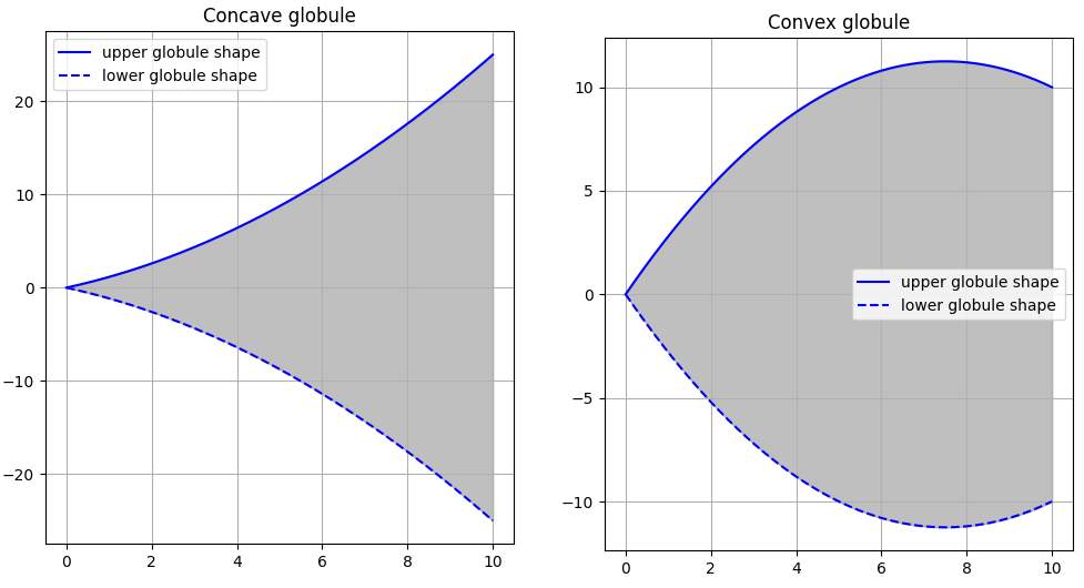
Figure 3. Schematic picture of a concave and a convex globule, on the left ($\delta>\check{\delta}(\beta)$) and right ($\delta<\check{\delta}(\beta)$) respectively.

3. Proof of Proposition 2.1: volume free energy

This section is devoted to the proof of Proposition 2.1, that is the existence of the (volume) free energy. Indeed, in statistical physics, the loss of analyticity in the free energy function indicates the presence of a phase transition. Extending the definition of the free energy in (1.6) to the case $\delta>0$ is not immediate since the sequence $(Z_{L,\beta,\delta})_{L\geq 1}$ is no longer trivially sub-additive in $L$. To that aim, we begin by defining the free energy as

Definition 3.1.

$$f(\beta,\delta):=\limsup_{L\to\infty}\frac{1}{L}\log Z_{L,\beta,\delta}\in\mathbb{R}.$$ (3.1)

To prove Proposition 2.1, we first need some classical results on a random walk representation, first stated in [14].

3.1. Random walk representation

Let $X:=(X_{i})_{i\geq 0}$ be a random walk on $\mathbb{Z}$ starting at the origin, with i.i.d. increments distributed as in (2.9). We will need to consider the geometric area enclosed between the random walk trajectory and the horizontal axis up to time $N$, as well as its arithmetic counterpart:

$$G_{N}(X):=\sum_{i=0}^{N}|X_{i}|\quad\text{and}\quad A_{N}(X):=\sum_{i=0}^{N}X_{i}.$$ (3.2)

Recall (1.1)–(1.5). For $A\subset\Omega_{L}$ we denote by $Z_{L,\beta,\delta}(A)$ the partition function restricted to those trajectories $\ell\in A$, i.e.,

$$Z_{L,\beta,\delta}(A)=\sum_{\ell\in A}e^{H_{L,\beta,\delta}(\ell)}.$$ (3.3)

For $N\in\mathbb{N}$ we define the one-to-one correspondence:

$$T_{N}:\{0\}\times{\mathcal{L}}_{N,L} \mapsto\{(X_{i})_{i=0}^{N}\in\{0\}\times\mathbb{Z}^{N}\colon\,G_{N}(X)=L-N\}$$

$$(\ell_{i})_{i=0}^{N} \mapsto((-1)^{i-1}\ell_{i})_{i=0}^{N}.$$ (3.4)

Then, any subset $A\subset\Omega_{L}$ is said to be stable by time inversion if for every $N\in\mathbb{N}$ we have that $(\ell_{i})_{i=1}^{N}\in A\cap{\mathcal{L}}_{N,L}$ implies $(\ell_{N+1-i})_{i=1}^{N}\in A\cap{\mathcal{L}}_{N,L}$.

Lemma 3.2.

Let $L\in\mathbb{N}$ and $A\subset\Omega_{L}$ be stable by time inversion. Then,

$$Z_{L,\beta,\delta}(A)=e^{\beta L}\,\underset{N=1}{\overset{L}{\sum}}\,\Gamma_{\beta}^{N}\,\mathbf{E}_{\beta}\Big{(}e^{(\delta-\frac{\beta}{2})|X_{N}|}1_{\{X\in T_{N}(A\cap{\mathcal{L}}_{N,L})\}}\Big{)}.$$ (3.5)

Proof of Lemma 3.2.

To begin with, we use the stability of $A$ by time inversion to get

$$Z_{L,\beta,\delta}(A) =\underset{N=1}{\overset{L}{\sum}}\,\sum_{\ell\in A\cap{\mathcal{L}}_{N,L}}e^{|\ell_{1}|\delta}\,\underset{i=1}{\overset{N-1}{\prod}}e^{\frac{\beta|\ell_{i}|+\beta|\ell_{i+1}|-\beta|\ell_{i}+\ell_{i+1}|}{2}}$$ (3.6)

$$=\underset{N=1}{\overset{L}{\sum}}\,\sum_{\ell\in A\cap{\mathcal{L}}_{N,L}}e^{|\ell_{N}|\delta}\,\underset{i=1}{\overset{N-1}{\prod}}e^{\frac{\beta|\ell_{i}|+\beta|\ell_{i+1}|-\beta|\ell_{i}+\ell_{i+1}|}{2}}.$$

For computational reasons, we add to every $\ell\in{\mathcal{L}}_{N,L}$ a zero-length stretch at the beginning of the configuration, that is, $\ell_{0}=0$. Thus,

$$Z_{L,\beta,\delta}(A)=e^{\beta L}\underset{N=1}{\overset{L}{\sum}}\Gamma_{\beta}^{N}\sum_{\ell\in A\cap{\mathcal{L}}_{N,L}}e^{|\ell_{N}|(\delta-\frac{\beta}{2})}\,\underset{i=0}{\overset{N-1}{\prod}}\frac{e^{-\frac{\beta|\ell_{i}+\ell_{i+1}|}{2}}}{c_{\beta}},$$ (3.7)

where $\Gamma_{\beta}=c_{\beta}\,e^{-\beta}$ and where we have used that $\sum_{i=1}^{N}|\ell_{i}|=L-N$. We observe that the product in the r.h.s. of (3.7) coincides with the probability that the random walk $X$ defined above follows the trajectory $X_{i}=(-1)^{i-1}\ell_{i}$ for $i\in\{0,\ldots,N\}$. Thus, (3.7) can be written as

$$Z_{L,\beta,\delta}(A)=e^{\beta L}\underset{N=1}{\overset{L}{\sum}}\Gamma_{\beta}^{N}\sum_{\ell\in A\cap{\mathcal{L}}_{N,L}}e^{|\ell_{N}|(\delta-\frac{\beta}{2})}\,\mathbf{P}_{\beta}\Big{(}X_{i}=(-1)^{i-1}\ell_{i},\ 0\leq i\leq N\Big{)},$$ (3.8)

Using the one-to-one correspondence $T_{N}$ defined in (3.1), we may conclude. ∎

3.2. Proof

In the core of the proof of Proposition 2.1 we will show that the $\limsup$ in (3.1) equals the $\liminf$, hence the convergence of the full sequence. We first prove Proposition 2.1 subject to Claim 3.3 and then prove Claim 3.3. We recall (2.9), (3.2) and for $x\in\mathbb{R}$, we define $x^{+}:=\max\{0,x\}$.

Claim 3.3.

For $u\leq\beta/2$ and $\gamma>0$, there exists $C>0$ such that, for every $N\geq 1$,

$$\mathbf{E}_{\beta}\Big{(}e^{u|X_{N}|}e^{-\gamma G_{N}(X)}\Big{)}\leq C\mathbf{E}_{\beta}\Big{(}e^{(u-\gamma)^{+}|X_{N-1}|}e^{-\gamma G_{N-1}(X)}\Big{)}.$$ (3.9)

with $X_{0}=G_{0}=0$.

Proof of Proposition 2.1.

We proceed with lim sup and lim inf successively. By (i) restricting the partition function to the path taking only one vertical stretch of length $L-1$ and (ii) noticing that $Z_{L,\beta,\delta}\geq Z_{L,\beta,0}$ for $L\in\mathbb{N}$ and $\delta\geq 0$, we get that

$$\underset{L\longrightarrow\infty}{\liminf}\frac{1}{L}\log Z_{L,\beta,\delta}\geq f(\beta,0)\vee\delta.$$ (3.10)

To complete the proof, it remains to consider lim sup instead of lim inf in (3.10). Therefore, we want to prove that:

$$f(\beta,\delta)\leq f(\beta,0)\vee\delta.$$ (3.11)

We first decompose the partition function according to the length of the first vertical stretch (either up or down) and add a reward $\beta$ along the whole second stretch, which gives us the following upper bound :

$$Z_{L,\beta,\delta}\leq 2\underset{k=0}{\overset{L-1}{\sum}}e^{k\delta}Z_{L-k-1,\beta,\beta}.$$ (3.12)

Hence, after taking the logarithm and dividing by the polymer length $L$ we obtain

$$\frac{1}{L}\log Z_{L,\beta,\delta}\leq\underset{0\leq k<L}{\max}\Big{\{}\tfrac{k}{L}\delta+(1-\tfrac{k+1}{L})\,\tfrac{1}{L-k-1}\,\log(Z_{L-k-1,\beta,\beta})\Big{\}}+o_{L}(1),$$ (3.13)

from which we deduce, after letting $L\to\infty$ that $f(\beta,\delta)\leq f(\beta,\beta)\vee\delta$. Thus, the proof will be complete once we show that $f(\beta,0)=f(\beta,\beta)$. To that aim, we start by applying the Cauchy-Hadamard Theorem, which guarantees us that for $(\beta,\delta)\in\mathcal{Q}$,

$$f(\beta,\delta)=\inf\Big{\{}\gamma\geq 0:\underset{L\geq 1}{\overset{}{\sum}}Z_{L,\beta,\delta}e^{-\gamma L}<\infty\Big{\}}.$$ (3.14)

Using Lemma 3.2 with $A=\Omega_{L}$ and the fact that $\{X\in T_{N}({\mathcal{L}}_{N,L})\}=\{G_{N}(X)=L-N\}$, we obtain for $\gamma\geq 0$,

$$\underset{L\geq 1}{\overset{}{\sum}}Z_{L,\beta,\delta}\,e^{-\gamma L} =\underset{N\geq 1}{\overset{}{\sum}}\underset{L\geq N}{\overset{}{\sum}}e^{-(\gamma-\beta)N}\,\Gamma_{\beta}^{N}\,\mathbf{E}_{\beta}\Big{(}e^{(\delta-\beta/2)|X_{N}|}1_{\{G_{N}(X)=L-N\}}e^{-(\gamma-\beta)(L-N)}\Big{)}$$ (3.15)

$$=\underset{N\geq 1}{\overset{}{\sum}}\left(\Gamma_{\beta}e^{-(\gamma-\beta)}\right)^{N}\mathbf{E}_{\beta}\Big{(}e^{(\delta-\beta/2)|X_{N}|}e^{-(\gamma-\beta)G_{N}(X)}\Big{)}.$$

We now pick $\delta=\beta$ and $\gamma>f(\beta,0)$. If we manage to prove that $\sum_{L\geq 1}Z_{L,\beta,\beta}e^{-\gamma L}<\infty$ then $f(\beta,\beta)\leq f(\beta,0)$ by (3.14), which would complete the proof (the reverse inequality clearly holds true). Using (3.15), it comes that:

$$\underset{L\geq 1}{\overset{}{\sum}}Z_{L,\beta,\beta}e^{-\gamma L}=\underset{N\geq 1}{\overset{}{\sum}}\left(\Gamma_{\beta}e^{-(\gamma-\beta)}\right)^{N}\mathbf{E}_{\beta}\Big{(}e^{(\beta/2)|X_{N}|}e^{-(\gamma-\beta)G_{N}(X)}\Big{)}.$$ (3.16)

We recall from (1.7) that $f(\beta,0)\geq\beta$ and therefore $\gamma-\beta>0$. Thus, we can denote by $k$ the smallest positive integer satisfying $\beta/2-k(\gamma-\beta)\leq 0$. It remains to successively use Claim 3.3 $k$ times to assert that there exists $C>0$, such that for $N\geq k$

$$\mathbf{E}_{\beta}\Big{(}e^{(\beta/2)|X_{N}|}e^{-(\gamma-\beta)G_{N}(X)}\Big{)}\leq C\ \mathbf{E}_{\beta}\Big{(}e^{-(\gamma-\beta)G_{N-k}(X)}\Big{)}.$$ (3.17)

As a consequence, there exists $C_{1}>0$ such that (3.16) becomes

$$\underset{L\geq 1}{\overset{}{\sum}}Z_{L,\beta,\beta}e^{-\gamma L} \leq C_{1}+C\underset{N\geq k}{\overset{}{\sum}}\left(\Gamma_{\beta}e^{-(\gamma-\beta)}\right)^{N}\mathbf{E}_{\beta}\Big{(}e^{-(\gamma-\beta)G_{N-k}(X)}\Big{)}$$ (3.18)

$$=C_{1}+C(\Gamma_{\beta}e^{\beta-\gamma})^{k}\underset{N\geq 0}{\overset{}{\sum}}\left(\Gamma_{\beta}e^{-(\gamma-\beta)}\right)^{N}\mathbf{E}_{\beta}\Big{(}e^{-(\gamma-\beta)G_{N}(X)}\Big{)}.$$

At this stage, we recall the following exponential growth rate from [1, Lemma 2.1]:

$$\mathfrak{h}_{\beta}(u):=\lim_{N\to\infty}\frac{1}{N}\log\mathbf{E}_{\beta}\Big{(}e^{-uG_{N}(X)}\Big{)}\leq 0,\quad u\in[0,\infty).$$ (3.19)

We now distinguish between two cases. If $\Gamma_{\beta}\leq 1$, then clearly $\log\Gamma_{\beta}-(\gamma-\beta)+\mathfrak{h}_{\beta}(\gamma-\beta)\leq-(\gamma-\beta)$, which is negative, since $\gamma>f(\beta,0)=\beta$. Assume now that $\Gamma_{\beta}>1$. Then, it was proven in [1, Theorem A] that

$$f(\beta,0)=\sup\{u\geq\beta\colon\log\Gamma_{\beta}-(u-\beta)+\mathfrak{h}_{\beta}(u-\beta)>0\}>\beta,$$ (3.20)

and that $f(\beta,0)$ is the only solution in $u$ of $\log\Gamma_{\beta}-(u-\beta)+\mathfrak{h}_{\beta}(u-\beta)=0$ (we pay attention to the fact that the excess free energy is $f(\beta,0)-\beta$). Since $\gamma>f(\beta,0)$ we necessarily have that $\log\Gamma_{\beta}-(\gamma-\beta)+\mathfrak{h}_{\beta}(\gamma-\beta)<0$ which implies that the r.h.s. in (3.18) is finite. This completes the proof. ∎

Proof of Claim 3.3.

Let $u\in(0,\beta/2]$ and $\gamma>0$. Since $G_{N}(X)-G_{N-1}(X)=|X_{N}|$,

$$\mathbf{E}_{\beta}\Big{(}e^{u|X_{N}|}e^{-\gamma G_{N}(X)}\Big{)}\leq\mathbf{E}_{\beta}\Big{(}e^{(u-\gamma)^{+}|X_{N}|}e^{-\gamma G_{N-1}(X)}\Big{)}.$$ (3.21)

If $u-\gamma\leq 0$, the claim readily follows. Otherwise, we use the triangular inequality, independence of the increments, and the fact that $u-\gamma<\beta/2$ to obtain as an upper bound:

$$\mathbf{E}_{\beta}\Big{(}e^{(u-\gamma)|X_{N}-X_{N-1}+X_{N-1}|}e^{-\gamma G_{N-1}(X)}\Big{)}$$ (3.22)

$$\leq\mathbf{E}_{\beta}\Big{(}e^{(u-\gamma)|X_{1}|}\Big{)}\mathbf{E}_{\beta}\Big{(}e^{(u-\gamma)|X_{N-1}|}e^{-\gamma G_{N-1}(X)}\Big{)}$$

$$\leq C\mathbf{E}_{\beta}\Big{(}e^{(u-\gamma)|X_{N-1}|}e^{-\gamma G_{N-1}(X)}\Big{)}.$$

This completes the proof. ∎

4. Preparation

4.1. Auxiliary partition functions

In what follows, for $q\geq 0$ and $\delta\in[0,\beta)$, we set

$$D_{N}(q,\delta): =\mathbf{E}_{\beta}\big{[}e^{(\delta-\frac{\beta}{2})X_{N}}\,1_{\{{\mathcal{V}}_{N,qN^{2},+}\}}\big{]},\qquad N\in\mathbb{N},$$ (4.1)

where

$${\mathcal{V}}_{N,k,+} =\{A_{N}=k,\ X_{i}>0,\ 0<i\leq N\},$$ (4.2)

and $A_{N}$ has been defined in (3.2). It turns out that $\psi(q,\delta)$ defined in (2.15) is the exponential growth rate of the sequence $(D_{N}(q,\delta))_{N\in\mathbb{N}}$. This result will be established as a byproduct of the proof of Proposition 4.22.

4.2. Bead decomposition

The aim of this section is to show how one can decompose a given trajectory in $\Omega_{L}$ into sub-trajectories that do not interact with each other, referred to as beads.

Note that we will extract some estimates from [11] where a similar decomposition has been introduced to study the same model when the wall-polymer interaction is shut-down ($\delta=0$). In the latter case, it was proven in [11, Theorem 2.2] that, inside the collapsed phase, a typical trajectory is made of a unique macroscopic bead from which only finitely many monomers may escape. In the present paper, although the uniqueness of the macroscopic bead still holds true inside the collapsed phase, the presence of an attractive wall both changes drastically the asymptotics of the partition function, but triggers also a much richer phenomenology including a surface transition and a radical change of the shape of the macroscopic bead.

The main difference between the model at $\delta>0$ and the model at $\delta=0$ is that in the former, the very first bead of a trajectory and the following beads need to be considered separately. The polymer-wall interaction indeed entails that, in large parts of the collapsed phase, the very first bead is the unique macroscopic bead. Therefore, deriving results on the polymer in this phase requires a deep understanding of most features of this first bead.

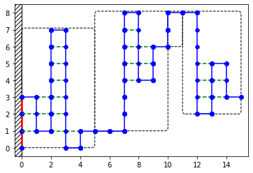
Figure 4. Bead decomposition of a trajectory. The blue lines stand for the polymer configuration, the orange dashed lines stand for the attractive self-interaction, and the red lines stand for the edges pinned at the attractive wall. In this example, we can see four beads each delimited by black dashed lines. The sign of the initial stretch of the third bead is determined by the last stretch of the previous bead. Since the second and fourth beads start with horizontal stretches, the sign of their first non-zero stretch may be either positive or negative.

Decomposition of a trajectory into beads

Let us start with a handful of notation. Set $\Omega^{\,\text{o}}:=\emptyset\cup(\cup_{L\geq 1}\,\Omega_{L}^{\,\text{o}})$ with $\Omega_{L}^{\,\text{o}}:=\cup_{N=1}^{L/2}\,{\mathcal{L}}_{N,L}^{\,\text{o}}$ where

$${\mathcal{L}}_{N,L}^{\,\text{o}}:=\Big{\{}(\ell_{i})_{i=1}^{N}\in\mathbb{Z}^{N}\colon\,\sum_{i=1}^{N}|\ell_{i}|=L-N,\ \ell_{i}\ell_{i+1}<0,\ \forall\,1\leq i<N\Big{\}},$$ (4.3)

so that $\Omega_{L}^{\,\text{o}}$ gathers those trajectories forming a unique bead of length $L$. The associated bead partition function is defined by

$$Z_{L,\beta,\delta}^{\,\text{o}}:=\sum_{\ell\in\Omega_{L}^{o}}e^{H_{L,\beta,\delta}(\ell)}=\sum_{N=1}^{L/2}Z_{L,\beta,\delta}({\mathcal{L}}_{N,L}^{\,\text{o}}).$$ (4.4)

Recall the definitions of $\Gamma_{\beta}$, $D_{N}(q,\delta)$ and ${\mathcal{V}}_{N,k,+}$ in (2.2), (4.1) and (4.2). By using Lemma 3.2 with $A={\mathcal{L}}_{N,L}^{\,\text{o}}$ and by noticing that $T_{N}$ (defined in (3.1)) is a one-to-one correspondance between ${\mathcal{L}}_{N,L}^{\,\text{o}}$ and ${\mathcal{V}}_{N,L-N,+}\cup{\mathcal{V}}_{N,L-N,-}$ we obtain that

$$\widetilde{Z}_{L,\beta,\delta}^{\,\text{o}}:=e^{-\beta L}Z_{L,\beta,\delta}^{\,\text{o}}=2\sum_{N=1}^{L/2}\Gamma_{\beta}^{N}D_{N}\big{(}\tfrac{L-N}{N^{2}},\delta\big{)}.$$ (4.5)

We now allow beads to start with stretches of zero length. To that aim, we define $\widehat{\Omega}^{\,\text{o}}:=\cup_{L\geq 1}\,\widehat{\Omega}_{L}^{\,\text{o}}$ where $\widehat{\Omega}_{L}^{\,\text{o}}:=\cup_{k=0}^{L-2}\,\widehat{\Omega}^{\text{o},k}_{L}$ with

$$\widehat{\Omega}_{L}^{\,\text{o},0} :=\{\ell\in\Omega_{L}^{\,\text{o}}\colon\,\ell_{1}>0\},$$ (4.6)

$$\widehat{\Omega}_{L}^{\,\text{o},k} :=\{\ell\in\Omega_{L}\colon\,N_{\ell}\geq k,\ \ell_{1}=\dots=\ell_{k}=0,\ (\ell_{i+k})_{i=1}^{N_{\ell}-k}\in\Omega_{L-k}^{\,\text{o}}\},\ k\in\mathbb{N}.$$

Those trajectories shall be called extended beads. Note that the condition $\ell_{1}>0$ in the first line of (4.6) is imposed by the fact that, when there is no zero-length stretch between two beads, the sign of the first vertical stretch of the second bead must correspond to that of the last stretch of the first bead. For the sake of simplicity, we define $\Omega^{c}_{L}$ as the subset of $\Omega_{L}$ that contains trajectories ending with a non-zero stretch, i.e.,

$$\Omega^{c}_{L}=\left\{\ell\in\Omega_{L}:\ell_{N_{\ell}}\neq 0\right\}.$$ (4.7)

With those subsets of trajectories in hand, we may divide a given trajectory as follows: $\tau_{0}:=0$ and for $j\in\mathbb{N}$ such that $\tau_{j-1}<N_{\ell}$,

$$\tau_{j}:=\tau_{j-1}+\max\{s>0\colon\,(\ell_{\tau_{j-1}+i})_{i=1}^{s}\in\widehat{\Omega}^{\,\text{o}}\quad\text{or}\quad(-\ell_{\tau_{j-1}+i})_{i=1}^{s}\in\widehat{\Omega}^{\,\text{o}}\}.$$ (4.8)

Finally, we let $n(\ell)$ be the number of (extended) beads into which a given trajectory $\ell\in\Omega_{L}$ may be divided. Thus, $\tau_{n(\ell)}=N_{\ell}$ and $\ell$ may be seen as the concatenation of $n(\ell)$ beads denoted by ${\mathcal{B}}_{j}:=(\ell_{\tau_{j-1}+1},\dots,\ell_{\tau_{j}})$, $j\in\{1,\dots,n_{\ell}\}$. The number of monomers in the $j$-th bead is denoted by $|{\mathcal{B}}_{j}|$ and has value $|{\mathcal{B}}_{j}|=\tau_{j}-\tau_{j-1}+\sum_{i=\tau_{j-1}+1}^{\tau_{j}}|\ell_{i}|$.

Bead decomposition of the partition function

We recall (4.4) and we note that only the first bead of the trajectory interacts with the vertical wall, provided that the trajectory does not begin with a horizontal stretch. This leads us to define

$$\bar{Z}_{L,\beta,\delta}^{\,\text{o}}:=Z_{L,\beta,\delta}^{\,\text{o}}+\sum_{k=1}^{L}Z_{L-k,\beta,0}^{\,\text{o}}=e^{\beta L}\widetilde{Z}_{L,\beta,\delta}^{\,\text{o}}+e^{\beta L}\sum_{k=1}^{L}e^{-\beta k}\widetilde{Z}_{L-k,\beta,0}^{\,\text{o}},$$ (4.9)

where $k$ stands for the number of initial stretches with zero length, as the contribution of the first (extended) bead to the partition function. The contribution of the following beads to the partition function does not involve $\delta$ since they cannot touch the vertical wall, leading us to define

$$\widehat{Z}_{L,\beta}^{\,\text{o}}:=\frac{1}{2}e^{\beta L}\widetilde{Z}_{L,\beta,0}^{\,\text{o}}+e^{\beta L}\sum_{k=1}^{L}e^{-\beta k}\widetilde{Z}_{L-k,\beta,0}^{\,\text{o}}.$$ (4.10)

Finally, we can decompose the full partition function $Z_{L,\beta,\delta}^{c}$, that is the partition function restrained to $\Omega^{c}_{L}$ according to the number of beads and the length of those beads, namely

$$Z_{L,\beta,\delta}^{c} =\sum_{k=1}^{L/2}\,\sum_{\begin{subarray}{c}t_{1}+\dots+t_{k}=L\\ t_{1},\ldots,t_{k}>1\end{subarray}}\,Z_{L,\beta,\delta}(n_{\ell}=k,|{\mathcal{B}}_{1}|=t_{1},\dots,|{\mathcal{B}}_{k}|=t_{k})$$ (4.11)

$$=\sum_{k=1}^{L/2}\,\sum_{\begin{subarray}{c}t_{1}+\dots+t_{k}=L\\ t_{1},\ldots,t_{k}>1\end{subarray}}\bar{Z}^{\,\text{o}}_{t_{1},\beta,\delta}\,\prod_{i=2}^{k}\widehat{Z}^{\,\text{o}}_{t_{i},\beta}.$$

Because of (4.11) above, proving Theorem 2.5 requires to derive both the asymptotics of the partition function sequence of the first bead, i.e., $(\bar{Z}_{L,\beta,\delta}^{\,\text{o}})_{L\in\mathbb{N}}$ and the asymptotics of the partition function of the following beads, namely $(\widehat{Z}_{L,\beta}^{\,\text{o}})_{L\in\mathbb{N}}$. The former is one of the main issue that we tackle in the present paper whereas the latter has been established in details in [11] and we recall it below.

Proposition 4.1 (Corollary 4.2 in [11]).

For $\beta>\beta_{c}$, there exists $K_{\beta}^{\text{o}},\widehat{K}_{\beta}^{\text{o}}>0$ such that

$$Z_{L,\beta,0}^{\,\text{o}} \underset{L\to\infty}{\sim}\frac{K_{\beta}^{\text{o}}}{L^{3/4}}\,e^{\beta L+g(\beta,0)\sqrt{L}}$$ (4.12)

$$\widehat{Z}_{L,\beta}^{\,\text{o}} \underset{L\to\infty}{\sim}\frac{\widehat{K}_{\beta}^{\text{o}}}{L^{3/4}}\,e^{\beta L+g(\beta,0)\sqrt{L}}$$

Remark 4.2.

Although in [11, Corollary 4.2] the prefactor in front of the $\sqrt{L}$ term in the exponential is expressed as $\widetilde{\mathcal{G}}(a_{\beta})$ and looks different from $g(\beta,0)$ that is used above, these two quantities are in fact equal to $\max\{T_{0}(a),a>0\}$ (see the definition of $T_{\delta}$ in Section 4.4 below). The expressions of $K_{\beta}^{\text{o}}$ and $\widehat{K}_{\beta}^{\text{o}}$ are available in [11, Equation (4.36)].

Remark 4.3.

As a non-trivial by-product of the proof of Theorem 2.5, we will prove in Lemma 6.13 that the beads which start with a non-zero vertical stretch bear all the mass coming from the extended beads in the partition function when $\delta\geq\delta_{c}(\beta)$, that is not only in the adsorbed-collapsed phase but also at criticality.

4.3. Change of measure

In this section we introduce several changes of measure for the position and area of the random walk that will be instrumental in deriving the asymptotics of the partition function.

Uniform tilting

We remind the reader that $\mathcal{L}$ is the logarithmic moment generating function of $X_{1}$ a random variable of law $\mathbf{P}_{\beta}$, defined in (2.10). That is a smooth, even and strictly convex function on $(-\beta/2,\beta/2)$ with a second derivative bounded from below by a positive constant. Let us first define a tilted transformation of $\mathbf{P}_{\beta}$. For $|h|<\beta/2$, we let $\widetilde{\mathbf{P}}_{h}$ be the probability law defined on $\mathbb{Z}$ by perturbing $\mathbf{P}_{\beta}$ as follows:

$$\frac{\text{d}\widetilde{\mathbf{P}}_{h}}{\text{d}\mathbf{P}_{\beta}}(\,\cdot\,=k)=e^{hk-\mathcal{L}(h)}\quad k\in\mathbb{Z}.$$ (4.13)

In the paper, we will consider the probability that a random walk $X:=(X_{i})_{i\in\mathbb{N}}$ starting from $x\in\mathbb{N}$ and with i.i.d. increments of law $\widetilde{\mathbf{P}}_{h}$ remains positive (or equivalently, that the random walk starting at the origin remains above level $-x$). To that aim, we state Lemma 4.4 below that will be proven in Section 7.1.

Lemma 4.4.

Let $\beta>0$. For every $x\in\mathbb{N}$ and $h\in(0,\beta/2)$, we have

$$\kappa^{x}(h):=\widetilde{\mathbf{P}}_{h}\Big{(}X_{i}>-x,\,\forall i\in\mathbb{N}\Big{)}=1-e^{-2hx}\frac{1-e^{h-\beta/2}}{1-e^{-h-\beta/2}},$$ (4.14)

that is continuous in $h$. Moreover, for every $c>0$ and $[h_{1},h_{2}]\subseteq(0,\beta/2)$,

$$\sup_{\begin{subarray}{c}0\leq x\leq c\log k\\ h\in[h_{1},h_{2}]\end{subarray}}\lim_{k\to\infty}|\widetilde{\mathbf{P}}_{h}\left(X_{[1,k]}>-x\right)-\kappa^{x}(h)|=0.$$ (4.15)

Tilting of the area enclosed by a random walk

We denote by $A_{n}(X)$ the algebraic area enclosed by $X$ up to time $n$, i.e.:

$$A_{n}(X)=X_{1}+...+X_{n}$$ (4.16)

and by $\Lambda_{n}$ the random vector recording the latter area renormalized by $n$ and the final position $X_{n}$ of the walk, that is,

$$\Lambda_{n}:=\left(\frac{A_{n}}{n},X_{n}\right).$$ (4.17)

Throughout the paper, we will need to estimate the probability of the event $\frac{1}{n}\Lambda_{n}=(q,p)\in\mathbb{R}^{2}$ and more importantly to work with the random walk conditioned on such events. To that aim, we will use an inhomogeneous exponential perturbation of the law of each increment of $X$, as it was first displayed in [5]. Thus, we define

$$\frac{\mathrm{d}\mathbf{P}_{n,\boldsymbol{h}}}{\mathrm{d}\mathbf{P}_{\beta}}(X)=e^{\boldsymbol{h}\cdot\Lambda_{n}-\mathcal{L}_{\Lambda_{n}}(\boldsymbol{h})}\quad\text{ with }\quad\mathcal{L}_{\Lambda_{n}}(\boldsymbol{h}):=\log\mathbf{E}_{\beta}\left[e^{\boldsymbol{h}\cdot\Lambda_{n}}\right]$$ (4.18)

where

$$\boldsymbol{h}\in\mathcal{D}_{\beta,n}:=\left\{\left(h_{0},h_{1}\right)\in\mathbb{R}^{2}\colon\Big{|}\tfrac{h_{0}}{n}+h_{1}\Big{|}<\beta/2,\ \left|h_{0}+h_{1}\right|<\beta/2\right\}.$$ (4.19)

Noticing that

$$\boldsymbol{h}\cdot\Lambda_{n}=\sum_{k=1}^{n}(X_{k}-X_{k-1})\Big{(}h_{0}[1-\tfrac{k-1}{n}]+h_{1}\Big{)},$$ (4.20)

we see that this change of measure corresponds to an inhomogeneous tilt on the increments of the random walk. We also set a continuous counterpart, namely

$$\mathcal{D}_{\beta}:=\left\{\left(h_{0},h_{1}\right)\in\mathbb{R}^{2}\colon\left|h_{1}\right|<\beta/2,\ \left|h_{0}+h_{1}\right|<\beta/2\right\},$$ (4.21)

and we observe that, by (4.20), the sequence $(\frac{1}{n}\mathcal{L}_{\Lambda_{n}}(\boldsymbol{h}))_{n\in\mathbb{N}}$ converges for any $\boldsymbol{h}\in\mathcal{D}_{\beta}$ (note that $\mathcal{D}_{\beta}\subseteq\mathcal{D}_{\beta,n}$ for every $n\in\mathbb{N}$) towards:

$$\mathcal{L}_{\Lambda}(\boldsymbol{h}):=\int_{0}^{1}\mathcal{L}\left(h_{0}x+h_{1}\right)\mathrm{d}x.$$ (4.22)

The two items of the following proposition come from [1, Lemma 5.4] and [1, Lemma 5.3] respectively. We take this occasion to correct a mistake in the original proof of  [1, Lemma 5.3], see Appendix E.

Proposition 4.5.

Let $\beta>0$.

1. For every $n\in\mathbb{N}$, the gradient $\nabla\left[\frac{1}{n}\mathcal{L}_{\Lambda_{n}}\right]$ is a $\mathcal{C}^{1}$-diffeomorphism from $\mathcal{D}_{\beta,n}$ to $\mathbb{R}^{2}$. For this reason, for $(q,p)\in\mathbb{R}^{2}$ there exists a unique

   $$\boldsymbol{h}:=\boldsymbol{h}_{n}(q,p)=(h_{n,0}(q,p),h_{n,1}(q,p))$$ (4.23)

   which solves:

   $$\mathbf{E}_{n,\boldsymbol{h}}\Big{[}\frac{1}{n}\Lambda_{n}\Big{]}=\nabla\Big{[}\frac{1}{n}\mathcal{L}_{\Lambda_{n}}\Big{]}(\boldsymbol{h})=(q,p).$$ (4.24)

2. $\nabla\mathcal{L}_{\Lambda}$ is a $\mathcal{C}^{1}$-diffeomorphism from $\mathcal{D}_{\beta}$ to $\mathbb{R}^{2}$. Thus, for $(q,p)\in\mathbb{R}^{2}$ we let $\widetilde{\boldsymbol{h}}(q,p)$ be the unique solution in $\boldsymbol{h}\in\mathcal{D}_{\beta}$ of the equation $\nabla\mathcal{L}_{\Lambda}(\boldsymbol{h})=(q,p)$.

Along the present paper we will need to consider two particular cases of the tilting procedure set up in (4.18), namely (i) a tilting for which the second coordinate in $\boldsymbol{h}$ is prescribed and (ii) a tilting for which $p=0$.

Case (i): The tilt on the final position is prescribed

This is the case where the value of $h_{1}$ is set to be $\delta-\beta/2$ (as suggested by Lemma 3.2). Let $\delta\in(0,\beta)$, $n\in\mathbb{N}$ and set

$${\mathcal{A}}_{n,\delta}:=\Big{(}-\frac{2n}{2n-1}\delta,\frac{2n}{2n-1}(\beta-\delta)\Big{)},$$

so that for $s\in{\mathcal{A}}_{n,\delta}$ and after recalling (4.18) we may consider the perturbed probability measure $\mathbf{P}_{n,(s,\delta-\frac{\beta}{2}-\frac{s}{2n})}$ . Note that the correction $\frac{s}{2n}$ in the second parameter is introduced as a technical artifact to obtain Proposition 4.8 below. To be more specific, we come back to (4.20) and write

$$\frac{\mathrm{d}\mathbf{P}_{n,(s,\delta-\frac{\beta}{2}-\frac{s}{2n})}}{\mathrm{d}\mathbf{P}_{\beta}}(X)=e^{(s,\delta-\frac{\beta}{2}-\frac{s}{2n})\cdot\Lambda_{n}-n\,{\mathcal{H}}_{n,\delta}(s)}$$ (4.25)

where

$${\mathcal{H}}_{n,\delta}(s)=\frac{1}{n}\,\mathcal{L}_{\Lambda_{n}}\Big{(}s,\delta-\frac{\beta}{2}{-\frac{s}{2n}}\Big{)},\quad s\in{\mathcal{A}}_{n,\delta}.$$ (4.26)

In what follows, we will need to tune $s\in{\mathcal{A}}_{n,\delta}$ in such a way that the expectation of $A_{n}$ equals $qn^{2}$ for some $q>0$. This is the object of Lemma 4.6 below, which guarantees the existence and uniqueness of such a parameter $s$. We extend this result to the continuous counterpart of ${\mathcal{H}}_{n,\delta}(s)$ that is, in view of (4.20),

$${\mathcal{H}}_{\delta}(s):=\int_{0}^{1}\mathcal{L}\Big{(}sx+\delta-\frac{\beta}{2}\Big{)}\,\mathrm{d}x,\quad s\in{\mathcal{A}}_{\delta}:=(-\delta,\beta-\delta),$$ (4.27)

where we observe that ${\mathcal{A}}_{\delta}\subseteq{\mathcal{A}}_{n,\delta}$ for every $n\geq 1$.

Lemma 4.6.

Let $\delta\in(0,\beta)$.

1. For every $n\geq 2$, the mapping ${\mathcal{H}}_{n,\delta}$ is $\mathscr{C}^{\infty}$ and strictly convex on ${\mathcal{A}}_{n,\delta}$. Moreover, ${\mathcal{H}}_{n,\delta}^{\prime}$ is a $\mathscr{C}^{1}$-diffeomorphism from ${\mathcal{A}}_{n,\delta}$ to $\mathbb{R}$.

2. The mapping ${\mathcal{H}}_{\delta}$ is $\mathscr{C}^{\infty}$ and strictly convex on ${\mathcal{A}}_{\delta}$. Moreover, the function ${\mathcal{H}}_{\delta}^{\prime}$ is a $\mathscr{C}^{1}$-diffeomorphism from ${\mathcal{A}}_{\delta}$ to $\mathbb{R}$.

3. The function ${\mathcal{H}}_{\delta}$ is bounded on ${\mathcal{A}}_{\delta}$.

Proof of Lemma 4.6.

The first item of Lemma 4.6 being a discrete counterpart of the second item, we will only prove the foremost here. Recalling that $\mathcal{L}$ is strictly convex and $\mathscr{C}^{\infty}$ on $(-\beta/2,\beta/2)$, it comes that ${\mathcal{H}}_{N,\delta}$ is also strictly convex and $\mathscr{C}^{\infty}$ as the finite sum of strictly convex and $\mathscr{C}^{\infty}$ functions. Moreover, ${\mathcal{H}}_{N,\delta}^{\prime}$ is increasing as the finite sum of increasing functions. Finally, since $\mathcal{L}^{\prime\prime}$ is bounded from below by a positive constant, we obtain that $\mathcal{L}^{\prime}(h)$ goes to $\pm\infty$ as $h\to\pm\beta/2$, respectively. Necessarily, ${\mathcal{H}}_{N,\delta}^{\prime}({\mathcal{A}}_{N,\delta})=\mathbb{R}$, which completes the proof. Let us now turn to the third item. It is sufficient to look at the function outside a neighborhood of the origin. A straightforward change of variable yields, provided $s\neq 0$:

$${\mathcal{H}}_{\delta}(s)=\int_{0}^{1}\mathcal{L}(sx+\delta-\beta/2)\mathrm{d}x\leq\frac{1}{|s|}\int_{-\beta/2}^{\beta/2}\mathcal{L}(x)\mathrm{d}x,$$ (4.28)

which proves our claim, since the last integral is finite. ∎

As a consequence of Lemma 4.6, we may define $s_{\delta,n}(q)$ and $s_{\delta}(q)$ for every $q>0$ as the respective solutions of

$${\mathcal{H}}_{n,\delta}^{\prime}(s)=q\quad\text{and}\quad{\mathcal{H}}_{\delta}^{\prime}(s)=q.$$ (4.29)

For $N\in\mathbb{N}$ and $q>0$ we will need in several instances to consider $\mathbf{P}_{N,\rm{sup}}^{\delta,q}$ the probability law on random walk trajectories displayed in (4.25) with $n=N$ and with parameter $s=s_{\delta,N}(q)$, i.e.,

$$\mathbf{P}_{N,\rm{sup}}^{\delta,q}=\mathbf{P}_{N,\big{(}s_{\delta,N}(q),\delta-\frac{\beta}{2}-\frac{s_{\delta,N}(q)}{2N}\big{)}}\,.$$ (4.30)

Remark 4.7.

Under $\mathbf{P}_{N,\rm{sup}}^{\delta,q}$ the increments of $X$, namely $X_{k}-X_{k-1}$ for $k\in\{1,\dots,N\}$ are independent and follow respectively the tilted law defined in (4.13) with tilt parameter $\delta-\frac{\beta}{2}+s_{\delta,N}(q)\frac{2N+1-2k}{2N}$.

The following proposition quantifies the convergence speed of ${\mathcal{H}}_{N,\delta}$ and $s_{\delta,N}(q)$ towards ${\mathcal{H}}_{\delta}$ and $s_{\delta}(q)$, respectively.

Proposition 4.8.

For every $[q_{1},q_{2}]\subseteq(0,\infty)$ and $[s_{1},s_{2}]\subseteq{\mathcal{A}}_{\delta}$, there exists $C>0$ and $N_{0}\in\mathbb{N}$ such that, for every $N\geq N_{0}$ and $s\in[s_{1},s_{2}]$:

$$|{\mathcal{H}}_{N,\delta}(s)-{\mathcal{H}}_{\delta}(s)|\leq\frac{C}{N^{2}}$$ (4.31)

and for every $q\in[q_{1},q_{2}]\cap\frac{\mathbb{N}}{N^{2}}$:

$$|s_{\delta,N}(q)-s_{\delta}(q)|\leq\frac{C}{N^{2}}.$$ (4.32)

The proof of Proposition 4.8 can be found in Appendix B.1. As we will see, the correction in $1/N^{2}$ is crucial in order to obtain the sharp asymptotics in Theorem 2.5, as well as in Lemma 4.9 below, the proof of which is deferred to Appendix B.2.

Lemma 4.9.

For every $B\in\sigma(X_{0},\dots,X_{N})$, for every $0<q_{1}<q_{2}<\infty$ and uniformly in $q\in[q_{1},q_{2}]$, as $N\to\infty$,

$$\mathbf{E}_{\beta}\Big{[}e^{(\delta-\frac{\beta}{2})X_{N}}1_{\{A_{N}=qN^{2},\,X\in B\}}\Big{]}=$$ (4.33)

$$\widetilde{c}e^{N\big{[}{\mathcal{H}}_{\delta}(s_{\delta}(q))-s_{\delta}(q)q\big{]}}\left(\mathbf{P}_{N,\rm{sup}}^{\delta,q}\left(A_{N}=qN^{2},X\in B\right)(1+o(1))+O(e^{-\log(N)^{2}})\right),$$

with $\widetilde{c}=\exp\Big{(}\frac{1}{2}\Big{[}{\mathcal{L}}(\delta-\beta/2+s_{\delta}(q))-{\mathcal{L}}(\delta-\beta/2)\Big{]}\Big{)}$.

Case (ii): The final position is set to zero.

This is the case where the value of the final position $p$ in Proposition 4.5 (1) equals $0$. For every $q>0$ and $n\in\mathbb{N}$ there exists a unique solution of $\nabla\left[\frac{1}{n}\mathcal{L}_{\Lambda_{n}}\right](\boldsymbol{h})=(q,0)$ denoted by $\boldsymbol{h}_{n}(q,0)=(h_{n,0}(q,0),h_{n,1}(q,0))$. However the fact that $\mathcal{L}$ is even entails that

$$h_{n,1}(q,0))=-\frac{h_{n,0}(q,0)}{2}\,\Big{(}1+\frac{1}{n}\Big{)}.$$ (4.34)

Equality (4.34), combined with (4.18) brings us to introduce a new probability law $\mathbf{P}_{n,h}$ on the random walk $X$ obtained as

$$\mathbf{P}_{n,h}:=\mathbf{P}_{n,\big{(}h,-\frac{1}{2}h(1+\frac{1}{n})\big{)}}\quad\text{for}\quad h\in\bigg{(}-\frac{n\beta}{n-1},\frac{n\beta}{n-1}\bigg{)}.$$ (4.35)

The normalisation constant of $\mathbf{P}_{n,h}$ may be expressed as $e^{-n\,{\mathcal{G}}_{n}(h)}$ with

$${\mathcal{G}}_{n}(h) :=\frac{1}{n}\mathcal{L}_{\Lambda_{n}}\left[h,-\frac{h}{2}\left(1+\frac{1}{n}\right)\right]\quad\text{ for }\quad h\in\left(-\frac{n\beta}{n-1},\frac{n\beta}{n-1}\right).$$ (4.36)

In view of (4.20), its continuous counterpart comes as

$${\mathcal{G}}(h):=\int_{0}^{1}\mathcal{L}\left(h\left(\frac{1}{2}-x\right)\right)\mathrm{d}x,\quad\text{ for }h\in(-\beta,\beta).$$ (4.37)

The following lemma can be seen as the particular case of Items (1) and (2) in Proposition 4.5 when $p=0$.

Lemma 4.10 (Lemma 5.3 in [11]).

Let $\beta>0$.

1. For $n\geq 2$, the mapping ${\mathcal{G}}_{n}$ is $\mathscr{C}^{2}$ and strictly convex on $(-\frac{n\beta}{n-1},\frac{n\beta}{n-1})$. Moreover, ${\mathcal{G}}_{n}^{\prime}$ is a $\mathscr{C}^{1}$-diffeomorphism from $(-\frac{n\beta}{n-1},\frac{n\beta}{n-1})$ to $\mathbb{R}$.

2. The mapping ${\mathcal{G}}$ is $\mathscr{C}^{2}$ and strictly convex on $(-\beta,\beta)$. Moreover, ${\mathcal{G}}^{\prime}$ is a $\mathscr{C}^{1}$-diffeomorphism from $(-\beta,\beta)$ to $\mathbb{R}$.

Remark 4.11.

For the sake of conciseness, for every $q\geq 0$ we set

$$h_{n}^{q}:=h_{n,0}(q,0)$$ (4.38)

and we let $\widetilde{h}(q)$ be the first coordinate of $\widetilde{\boldsymbol{h}}(q,0)$ that we introduced in Proposition 4.5 (2). Once again, because $\mathcal{L}$ is even we observe that the continuous counterpart of (4.34) holds true, i.e.,

$$\boldsymbol{\tilde{h}}(q,0)=\Big{(}\widetilde{h}(q),-\frac{\widetilde{h}(q)}{2}\Big{)}.$$ (4.39)

The functions $q\mapsto h_{n}^{q}$ and $q\mapsto\widetilde{h}(q)$ are consequently the restrictions to $(0,\infty)$ of the inverse functions of ${\mathcal{G}}_{n}^{\prime}$ and ${\mathcal{G}}^{\prime}$. As a consequence of Lemma 4.10 the function $q\longrightarrow\widetilde{h}(q)$ is increasing.

We finally observe that the exponential tilt of $\mathbf{P}_{n,h}$ may be expressed as

$$\frac{\mathrm{d}\mathbf{P}_{n,h}}{\mathrm{\leavevmode\nobreak\ d}\mathbf{P}_{\beta}}(X)=e^{-\psi_{n,h}\left(A_{n},X_{n}\right)},\text{ with }\psi_{n,h}(a,x):=-\frac{h}{n}a+\frac{h}{2}\left(1+\frac{1}{n}\right)x+n{\mathcal{G}}_{n}(h),\quad x,a\in\mathbb{Z}.$$ (4.40)

As in the previous case, Proposition 4.12 below provides the convergence speed of the discrete quantities ${\mathcal{G}}_{N}(h)$ and $h_{N}^{q}$ towards ${\mathcal{G}}(h)$ and $\widetilde{h}(q)$ respectively.

Proposition 4.12 (Propositions 5.1 and 5.4 in [11]).

For every $[q_{1},q_{2}]\subseteq(0,\infty)$ and $[h_{1},h_{2}]\subseteq(-\beta,\beta)$, there exists $C>0$ and $N_{0}\in\mathbb{N}$ such that, for every $N\geq N_{0}$ and $h\in[h_{1},h_{2}]$:

$$|{\mathcal{G}}_{N}(h)-{\mathcal{G}}(h)|\leq\frac{C}{N^{2}}\ ,$$ (4.41)

and for every $q\in[q_{1},q_{2}]\cap\frac{\mathbb{N}}{N^{2}}$:

$$|h_{N}^{q}-\widetilde{h}(q)|\leq\frac{C}{N^{2}}.$$ (4.42)

Remark 4.13 (Time-reversal property).

If $|h|<\beta/2$ and $Z$ is distributed as $\widetilde{\mathbf{P}}_{h}$, as in (4.13), then one can check that $-Z$ is distributed as $\widetilde{\mathbf{P}}_{-h}$. Recalling (4.20) we note that under $\mathbf{P}_{n,h}$, the increments of $X$, namely $X_{k}-X_{k-1}$ for $k\in\{1,\dots,N\}$ are independent and follow respectively the tilted law $\widetilde{\mathbf{P}}_{\frac{h}{2}\left(1-\frac{2k-1}{n}\right)}$. Therefore, $X$ is time-reversible, i.e.,

$$\left(X_{k}\right)_{k=0}^{n}\underset{\text{(law)}}{=}\left(X_{n-k}-X_{n}\right)_{k=0}^{n}$$ (4.43)

We deduce therefrom that the random walk $X$ distributed as $\mathbf{P}_{n,h}$ is an inhomogeneous Markov chain that satisfies for all $j\in\{1,\ldots,n-1\}$ and $y\in\mathbb{Z}$,

$$\mathbf{P}_{n,h}\left(\left(X_{j+k}\right)_{k=1}^{n-j-1}\in\cdot\ ,\ X_{n}=0\mid X_{j}=y\right)=\mathbf{P}_{n,h}\left(\left(X_{n-j-k}\right)_{k=1}^{n-j-1}\in\cdot\ ,\ X_{n-j}=y\right).$$ (4.44)

Finally, note that the case $h=0$ corresponds to the random walk $X$ with i.i.d. increments of law $\mathbf{P}_{\beta}$.

4.4. Analysis of auxiliary functions

In this section we analyse the function $\psi$ displayed in (2.15) and the function

$$T_{\delta}:a\in(0,\infty)\mapsto a\log\Gamma_{\beta}+a\psi(\tfrac{1}{a^{2}},\delta),$$ (4.45)

which play a key role in deriving the asymptotic behaviour of the auxiliary partition functions in (4.1) and ultimately expressing the surface free energy as a variational formula, see (2.19).

Let us start with the regularity properties of $\psi$. Recalling the two cases in (2.15), we first define, for every $0\leq\delta<\beta$:

$$q_{\delta}:=\inf\Big{\{}q>0\colon\delta>\delta_{0}(q)=\tfrac{\beta}{2}-\tfrac{\widetilde{h}(q)}{2}\Big{\}}.$$ (4.46)

Two cases arise:

1. If $0\leq\delta<\beta/2$ then, by Remark 4.11, $q_{\delta}$ is actually the unique solution in $q>0$ of ${\widetilde{h}(q)}/{2}={\beta}/{2}-\delta$ and, by definition of $\widetilde{h}(q)$, we have the following explicit expression:

   $$q_{\delta}:=\int_{0}^{1}(x-\tfrac{1}{2})\mathcal{L}^{\prime}\Big{(}(\tfrac{\beta}{2}-\delta)(2x-1)\Big{)}\mathrm{d}x.$$ (4.47)

   Note that the factor $x-1/2$ in (4.47) may be replaced by $x$, since $\mathcal{L}^{\prime}$ is odd. Moreover, the cases $\delta\leq\delta_{0}(q)$ and $\delta>\delta_{0}(q)$ in the expression of $\psi$, see (2.15), correspond to $q\leq q_{\delta}$ and $q>q_{\delta}$, respectively.

2. If $\beta/2\leq\delta<\beta$ then the inequality in (4.46) is always true, hence $q_{\delta}=0$ and, from (2.15), $\psi(q,\delta)={\mathcal{H}}_{\delta}(s_{\delta}(q))-qs_{\delta}(q)$ for every $q>0$.

Lemma 4.14.

Let $0\leq\delta<\beta$. The mapping $q\mapsto\psi(q,\delta)$ is $\mathscr{C}^{1}$ on $(0,\infty)$. Moreover, it is $\mathscr{C}^{2}$ on $(0,q_{\delta})\cup(q_{\delta},\infty)$ if $0<\delta<\beta/2$ (in which case $q_{\delta}>0)$ and it is $\mathscr{C}^{2}$ on $(0,\infty)$ if $\beta/2\leq\delta<\beta$ (in which case $q_{\delta}=0)$.

Proof of Lemma 4.14.

By (2.16) and (2.15),

$$\psi(q,\delta)={1}_{\{\frac{\widetilde{h}(q)}{2}\leq\frac{\beta}{2}-\delta\}}\ \big{(}{\mathcal{G}}(\widetilde{h}(q))-q\widetilde{h}(q)\big{)}+{1}_{\{\frac{\widetilde{h}(q)}{2}>\frac{\beta}{2}-\delta\}}\ \big{(}{\mathcal{H}}_{\delta}(s_{\delta}(q))-qs_{\delta}(q)\big{)}.$$ (4.48)

Since, by Lemmas 4.10 and 4.6, both functions $q\mapsto{\mathcal{G}}(\widetilde{h}(q))-q\widetilde{h}(q)$ and $q\mapsto{\mathcal{H}}_{\delta}(s_{\delta}(q))-qs_{\delta}(q)$ are $\mathscr{C}^{2}$ on $(0,\infty)$, it is sufficient to show that the first derivatives coincide at $q_{\delta}$. Indeed, we compute, when $q\in(0,q_{\delta})$,

$$(\partial_{q}\psi)(q,\delta)=\widetilde{h}^{\prime}(q){\mathcal{G}}^{\prime}(\widetilde{h}(q))-q\widetilde{h}^{\prime}(q)-\widetilde{h}(q)=-\widetilde{h}(q),$$ (4.49)

and when $q\in(q_{\delta},\infty)$,

$$(\partial_{q}\psi)(q,\delta)=\partial_{q}(s_{\delta}(q))({\mathcal{H}}_{\delta})^{\prime}(s_{\delta}(q))-q\partial_{q}(s_{\delta}(q))-s_{\delta}(q)=-s_{\delta}(q).$$ (4.50)

We may now check that the first derivatives coincide at $q_{\delta}$. Indeed, one can verify that ${\mathcal{H}}^{\prime}_{\delta}(\widetilde{h}(q_{\delta}))={\mathcal{H}}^{\prime}_{\delta}(\beta-2\delta)=q_{\delta}$, by (4.47). As for the second derivatives, we obtain

$$(\partial^{2}_{q}\psi)(q,\delta)=\begin{cases}\widetilde{h}^{\prime}(q)&q\in(0,q_{\delta}),\\ s_{\delta}^{\prime}(q)&q\in(q_{\delta},\infty).\end{cases}$$ (4.51)

∎

Let us now turn to the properties of the function $T_{\delta}$ defined in (4.45). In the rest of the paper we often jump from one dummy variable $a\in(0,\infty)$ to another dummy variable $q\in(0,\infty)$ via the relation $q=1/a^{2}$. First, we focus on the concavity of the function. To this end, we define:

$$q^{*}_{\delta}:=\inf\{q>0\colon\delta-\beta/2+s_{\delta}(q)\geq 0\}$$ (4.52)

and notice that

$${\mathcal{H}}^{\prime}_{\delta}(\beta/2-\delta)=\int_{0}^{1}x\mathcal{L}^{\prime}((\delta-\beta/2)(1-x))\mathrm{d}x,$$ (4.53)

which implies, since $\mathcal{L}$ is odd, that

$$\textrm{sign}({\mathcal{H}}^{\prime}_{\delta}(\beta/2-\delta))=\textrm{sign}(\delta-\beta/2).$$ (4.54)

We may now distinguish between two cases:

1. If $0<\delta\leq\beta/2$ then ${\mathcal{H}}_{\delta}^{\prime}(\beta/2-\delta)\leq 0$, hence $s_{\delta}(0)\geq\beta/2-\delta$, by Lemma 4.6. Since $s_{\delta}$ is increasing, $\delta-\beta/2+s_{\delta}(q)\geq 0$ for every $q>0$, and $q^{*}_{\delta}=0$.

2. If $\beta/2<\delta<\beta$ then ${\mathcal{H}}_{\delta}^{\prime}(\beta/2-\delta)>0$, hence $s_{\delta}(0)<\beta/2-\delta$. Therefore, $q_{\delta}^{*}$ is the only solution in $q>0$ of the equation $\delta-\beta/2+s_{\delta}(q)=0$.

Lemma 4.15 (Concavity/Convexity).

For every $\beta>\beta_{c}$ and $\delta<\beta$, the function $T_{\delta}$ is $\mathscr{C}^{1}$ on $(0,\infty)$. It is $\mathscr{C}^{2}$ on $(0,1/\sqrt{q_{\delta}})\cup(1/\sqrt{q_{\delta}},\infty)$ if $0<\delta<\beta/2$ and it is $\mathscr{C}^{2}$ on $(0,\infty)$ if $\beta/2\leq\delta<\beta$. If $\delta\leq\beta/2$ (in which case $q^{*}_{\delta}=0$) it is strictly concave on $(0,\infty)$. If $\beta/2<\delta<\beta$ (in which case $q^{*}_{\delta}>0$) then it is strictly concave on $(0,1/\sqrt{q^{*}_{\delta}})$ and strictly convex on $(1/\sqrt{q^{*}_{\delta}},\infty)$.

The proof can be found in Appendix A.1 The next step is to determine the limits of $T_{\delta}(a)$ when $a\to 0$ and $a\to+\infty$. Recall that the parameter $a$ stands for the prescribed horizontal extension ($L=qN^{2}$ hence $N=a\sqrt{L}$ from (4.1) and (4.2)). This step is important to restrict the set of possible horizontal extensions to a compact set, see Section 4.7. To this end, we first notice that for every $|x|<\beta/2$, the map $\delta\mapsto{\mathcal{H}}^{\prime}_{\delta}(\beta/2-\delta-x)$ is increasing. Indeed, its derivative writes:

$$\int_{0}^{1}t(1-t)\mathcal{L}^{\prime\prime}((\beta/2-\delta-x)t+\delta-\beta/2)\mathrm{d}t>0,$$ (4.55)

which is positive, by strict convexity of $\mathcal{L}$. Recall the definitions of ${\mathcal{C}}_{\rm{good}}$ and $\bar{\delta}(\beta)$ in (2.17) and (2.18).

Lemma 4.16 (Limits).

For every $0<\delta<\beta$, $T_{\delta}(a)$ converges to $-\infty$ as $a\to 0$. For every $0<\delta<\bar{\delta}(\beta)$, $T_{\delta}(a)$ converges to $-\infty$ as $a\to+\infty$ and for every $\bar{\delta}(\beta)<\delta<\beta$ (provided this case is not empty), $T_{\delta}(a)$ converges to $+\infty$ as $a\to+\infty$.

The proof of this lemma can be found in Appendix A.2. As an immediate corollary of Lemma 4.15 and Lemma 4.16, we obtain:

Corollary 4.17.

If $(\beta,\delta)\in{\mathcal{C}}_{\rm{good}}$ then $T_{\delta}$ admits a unique maximizer on $(0,\infty)$.

In view of Lemma 4.16, a natural question is to determine for which values of $\beta$ we have $\bar{\delta}(\beta)<\beta$, respectively $\bar{\delta}(\beta)=\beta$. This is the content of the following lemma.

Lemma 4.18.

If $\beta>\beta_{c}$ is close enough to $\beta_{c}$ then $\beta/2\leq\bar{\delta}(\beta)<\beta$. However, there exists $\beta_{*}>\beta_{c}$ such that $\bar{\delta}(\beta)=\beta$ for every $\beta\geq\beta_{*}$.

The proof of Lemma 4.18 can be found in Appendix A.3. Numerically, we have $\beta_{c}\approx 1,219$ and $\beta_{*}\leq\pi/\sqrt{3}\approx 1,814$ (see the proof of Lemma A.13). As a straightforward consequence of Lemma 4.18, the set $\mathcal{C}_{\text{bad}}:={\mathcal{C}}\setminus{\mathcal{C}}_{\text{good}}$ defined in (2.17) is bounded.

Let us now make a few remarks on the maximizer of $q\mapsto T_{\delta}(1/\sqrt{q})$ when $(\beta,\delta)\in{\mathcal{C}}_{\rm{good}}$. First, we observe that:

Lemma 4.19.

For every $q\geq 0$:

$${\mathcal{H}}_{\delta}(s_{\delta}(q))=\mathcal{L}(s_{\delta}(q)+\delta-\beta/2)-qs_{\delta}(q);$$ (4.56)

$${\mathcal{G}}(\widetilde{h}(q))=\mathcal{L}({\widetilde{h}(q)}/{2})-q\widetilde{h}(q).$$ (4.57)

Proof of Lemma 4.19.

An integration by part gives:

$${\mathcal{H}}_{\delta}(s)=\int_{0}^{1}\mathcal{L}(st+\delta-\beta/2)\mathrm{d}t =[t\mathcal{L}(st+\delta-\beta/2)]_{0}^{1}-s\int_{0}^{1}t\mathcal{L}^{\prime}(st+\delta-\beta/2)\mathrm{d}t$$ (4.58)

$$=\mathcal{L}(s+\delta-\beta/2)-s{\mathcal{H}}_{\delta}^{\prime}(s),$$

and (4.56) readily follows from (2.14). A similar computation combined with (2.12) gives (4.57). ∎

Combining the derivative of $T_{\delta}$ in (A.1) and (A.2) with Lemma 4.19, we get that

$$T_{\delta}^{\prime}(1/\sqrt{q})=\begin{cases}\log\Gamma_{\beta}+\mathcal{L}(s_{\delta}(q)+\delta-\beta/2)&(q>q_{\delta})\\ \log\Gamma_{\beta}+\mathcal{L}(\widetilde{h}(q)/2)&(q<q_{\delta}).\end{cases}$$ (4.59)

These observations lead to the following:

Remark 4.20 (On the maximizer of $T_{\delta}$).

If $(\beta,\delta)\in{\mathcal{C}}_{\rm{good}}$ then the unique maximizer of $q\mapsto T_{\delta}(1/\sqrt{q})$, that we denote by $\bar{q}_{\beta,\delta}$, satisfies $\bar{q}_{\beta,\delta}=\bar{q}_{\beta,0}$ and $-\log\Gamma_{\beta}=\mathcal{L}(\widetilde{h}(\bar{q}_{\beta,0})/2)$ if $(\beta,\delta)\in{\mathcal{D}}{\mathcal{C}}$ and $-\log\Gamma_{\beta}=\mathcal{L}(s_{\delta}(\bar{q}_{\beta,\delta})+\delta-\beta/2)$ if $(\beta,\delta)\in{\mathcal{A}}{\mathcal{C}}$.

To close this section, we shortly come back to the function $\psi$ and state a lemma that will be essential for computing the order of the surface transition. Recall that $\delta_{0}(q)=\frac{\beta}{2}-\frac{\widetilde{h}(q)}{2}$.

Lemma 4.21.

For $(\beta,\delta)\in{\mathcal{C}}$ and $q>0$ such that $\delta>\delta_{0}(q)$ it holds that $\psi(q,\delta)>\psi(q,0)$. Moreover, as $\varepsilon\to 0^{+}$,

$$\psi(q,\delta_{0}(q)+\varepsilon)-\psi(q,0)\sim C\varepsilon^{2},$$ (4.60)

where $C=\frac{\mathcal{L}^{\prime}(\widetilde{h}(q)/2)(\mathcal{L}^{\prime}(\widetilde{h}(q)/2)-4q)}{2\widetilde{h}(q)(\mathcal{L}^{\prime}(\widetilde{h}(q)/2)-2q)}>0$.

The detailed proof is deferred to Appendix D.1.

4.5. Sharp asymptotics of auxiliary partition functions

In Proposition 4.22 below, we provide sharp asymptotics for the auxiliary partition function introduced in Section 4.1, in each of the three (desorbed, critical and adsorbed) regimes lying in the collapsed phase. Its proof is postponed to Section 7. Beforehand, we define $\vartheta:(-\beta/2,\beta/2)\rightarrow\mathbb{R}$ as:

$$\vartheta(h)=\int_{0}^{1}x^{2}\mathcal{L}^{\prime\prime}\Big{(}h\Big{(}x-\frac{1}{2}\Big{)}\Big{)}\mathrm{d}x\int_{0}^{1}\mathcal{L}^{\prime\prime}\Big{(}h\Big{(}x-\frac{1}{2}\Big{)}\Big{)}\mathrm{d}x-\left[\int_{0}^{1}x\mathcal{L}^{\prime\prime}\Big{(}h\Big{(}x-\frac{1}{2}\Big{)}\Big{)}\mathrm{d}x\right]^{2}\,.$$ (4.61)

We also recall the definitions of $\kappa^{x}(h)$ in (4.14), $\psi$ in (2.15), $\delta_{0}(q)$ in (2.16), and $q^{*}_{\delta}$ in (4.52).

Proposition 4.22.

Let $\beta>\beta_{c}$ and $0<q_{1}<q_{2}<\infty$.

1. For $\delta<\min\{\delta_{0}(q)\colon\;q\in[q_{1},q_{2}]\}$,

   $$D_{N}(q,\delta)=\frac{C_{\beta,q,\delta}}{N^{2}}e^{N{\psi}(q,0)}(1+o(1)),$$ (4.62)

   where $o(1)$ is uniform in $q\in(q_{1},q_{2})$, and

   $$C_{\beta,q,\delta}=\frac{\kappa^{0}\big{(}\tfrac{\widetilde{h}(q)}{2}\big{)}}{2\pi\vartheta(\widetilde{h}(q))^{\frac{1}{2}}}\left(\frac{1}{1-e^{\widetilde{u}}}-\frac{1-\kappa^{0}\big{(}\frac{\widetilde{h}(q)}{2}\big{)}}{1-e^{\widetilde{u}-\widetilde{h}(q)}}\right),$$ (4.63)

   with $\widetilde{u}:=\delta-\delta_{0}(q)$.

2. For $q\in(q_{1},q_{2})$ and $\delta=\delta_{0}(q)$, for all $R\geq 0$ and uniformly over $c\in[-R,R]$

   $$D_{N}(q+\tfrac{c}{\sqrt{N}},\delta)=\frac{C_{\beta,q,c}^{\rm{crit}}}{N^{3/2}}e^{N\psi(q,0)-\widetilde{h}(q)c\sqrt{N}}(1+o(1)),$$ (4.64)

   where $o(1)$ is uniform in $q\in(q_{1},q_{2})$, and

   $$C_{\beta,q,c}^{\rm{crit}}=\kappa^{0}(\widetilde{h}(q)/2)\int_{0}^{\infty}f_{\widetilde{h}(q)}(c,z)\mathrm{d}z,$$ (4.65)

   with $f_{\widetilde{h}(q)}$ defined in (4.74).

3. For $\delta>0$ and $[q_{1},q_{2}]\subset(q^{*}_{\delta},+\infty)$ such that $\delta>\delta_{0}(q_{1})$. We have the following estimate:

   $$D_{N}(q,\delta)=\kappa^{0}\big{(}\widetilde{h}(q)\big{)}\frac{\xi(q,\delta)}{N^{3/2}}e^{N\psi(q,\delta)}(1+o(1)),$$ (4.66)

   where the $o(1)$ is uniform over $q\in(q_{1},q_{2})$, and

   $$\xi(q,\delta):=\frac{e^{\mathcal{L}(\delta-\frac{\beta}{2}+s_{\delta}(q))-\mathcal{L}(\delta-\frac{\beta}{2})}}{\sqrt{2\pi\int_{0}^{1}x^{2}\mathcal{L}^{\prime\prime}\Big{(}\delta-\frac{\beta}{2}+s_{\delta}(q)x\Big{)}\mathrm{d}x}}.$$ (4.67)

In our way of proving Theorem 2.3, we shall need to check the assumption in Item (3) of Proposition 4.22. To this end, we can rely on the following lemma:

Lemma 4.23.

If $(\beta,\delta)\in{\mathcal{C}}_{\rm{good}}$ then the maximizer of $q\mapsto T_{\delta}(1/\sqrt{q})$ is larger than $q^{*}_{\delta}$.

Proof of Lemma 4.23.

If $\delta\leq\beta/2$ there is nothing to prove since then $q^{*}_{\delta}=0$ by Item (1) below (4.54). Now assume that $\beta/2<\delta<\beta$. By the definition of $q_{\delta}^{*}$ in (4.52) and Remark 4.20, when $\delta\geq\beta/2$, we have $s_{\delta}(q_{\delta}^{*})+\delta-\beta/2=0$, and the maximizer $\bar{q}_{\beta,\delta}$ satisfies $\mathcal{L}(s_{\delta}(\bar{q}_{\beta,\delta})+\delta-\beta/2)=-\log\Gamma_{\beta}>0$. Because both $q\in\mathbb{R}_{+}\mapsto s(q)$ and $x\in[0,\beta/2]\mapsto\mathcal{L}(x)$ are increasing functions, and since $\mathcal{L}(0)=0$, this proves that $\bar{q}_{\beta,\delta}>q_{\delta}^{*}$. ∎

Finally, Lemma 4.24 gives a uniform control on the sequence $(D_{N}(q,\delta))_{N\geq 1}$:

Lemma 4.24.

Let $q_{2}>0$. There exists $c>0$ such that for every $N\in\mathbb{N}$ and $q\in(0,q_{2}]$,

$$D_{N}(q,\delta)\leq c\,e^{N\psi(q,\delta)}.$$ (4.68)

Proof of Lemma 4.24.

We distinguish between two cases.
(i) If $\delta_{0}(q)<\delta\leq\beta$, we obtain with the help of Lemma 4.9:

$$D_{N}(q,\delta)=\mathbf{E}_{\beta}\Big{[}e^{(\delta-\frac{\beta}{2})X_{N}}1_{\{{\mathcal{V}}_{N,qN^{2},+}\}}\Big{]} \leq({\rm{cst.}})\mathbf{P}_{N,\rm{sup}}^{\delta,q}\left({\mathcal{V}}_{N,qN^{2},+}\right)\ e^{N\big{[}{\mathcal{H}}_{N,\delta}(s_{q}^{\delta})-s_{q}^{\delta}q\big{]}}$$ (4.69)

$$\leq({\rm{cst.}})\,e^{N\big{[}{\mathcal{H}}_{N,\delta}(s_{q}^{\delta})-s_{q}^{\delta}q\big{]}}.$$

It remains to apply (4.32) in Proposition 4.8 to conclude that for $N$ large enough, and for $q\in[q_{1},q_{2}]$,

$$e^{N\big{[}{\mathcal{H}}_{N,\delta}(s_{q}^{\delta})-s_{q}^{\delta}q\big{]}} \leq 2e^{N\big{[}{\mathcal{H}}_{\delta}(s_{q}^{\delta})-s_{q}^{\delta}q\big{]}}=2e^{\psi(q,\delta)N}.$$ (4.70)

(ii) If $0\leq\delta\leq\delta_{0}(q)$, we apply the tilting in (4.18) with $\boldsymbol{h}=(\widetilde{h}(q),-\frac{\widetilde{h}(q)}{2})$ to get

$$D_{N}(q,\delta) =\mathbf{E}_{\beta}\Big{[}e^{(\delta-\frac{\beta}{2})X_{N}}1_{\{{\mathcal{V}}_{N,qN^{2},+}\}}\Big{]}$$ (4.71)

$$=\mathbf{E}_{N,\widetilde{h}(q),-\frac{1}{2}\widetilde{h}(q)}\Big{[}e^{(\delta-\delta_{0}(q))X_{N}}1_{\{{\mathcal{V}}_{N,qN^{2},+}\}}\Big{]}\ e^{N\big{[}{\mathcal{G}}_{N}(\widetilde{h}(q))-\widetilde{h}_{q}q\big{]}}$$

$$\leq e^{N\big{[}{\mathcal{G}}_{N}(\widetilde{h}(q))-\widetilde{h}_{q}q\big{]}},$$

where we have used that $X\in{\mathcal{V}}_{N,q,+}$ necessarily implies $X_{N}\geq 0$. Using (4.41) in Proposition 4.12, together with the continuity of $q\mapsto\widetilde{h}(q)$, there exists an $N_{0}\in\mathbb{N}$ such that uniformly in $q\in[0,q_{2}]$, for $N\geq N_{0}$,

$$e^{N\big{[}{\mathcal{G}}_{N}(\widetilde{h}(q))-\widetilde{h}_{q}q\big{]}} \leq 2e^{N\big{[}{\mathcal{G}}(\widetilde{h}(q))-\widetilde{h}(q)q\big{]}}=2e^{\psi(q,\delta)N}.$$ (4.72)

This completes the proof. ∎

4.6. Local limits

The last main tool that we will use throughout the paper are Gnedenko-type local limit theorems. In this section, we present three theorems of that type involving $A_{N}$ and $X_{N}$, and introduce a change of measure used in the $\mathcal{AC}$ phase.

Local limit inside $\mathcal{DC}$ phase and at the critical curve

We recall the definitions of $\mathcal{L}_{\Lambda}$ in (4.22) and of ${\mathcal{D}}_{\beta}$ in (4.21). For every $\mathbf{h}\in{\mathcal{D}}_{\beta}$, we define the matrix

$$\mathbf{B}(\mathbf{h}):=\text{Hess }\mathcal{L}_{\Lambda}(\mathbf{h})$$ (4.73)

and the following Gaussian probability density:

$$f_{\mathbf{h}}:z\in\mathbb{R}^{2}\mapsto\frac{1}{2\pi\sqrt{\det\mathbf{B}(\mathbf{h})}}\exp\left(-\frac{1}{2}\langle\mathbf{B}(\mathbf{h})^{-1}z,z\rangle\right).$$ (4.74)

Recall the definition of $\boldsymbol{\tilde{h}}(q,0)$ in (4.39). The following proposition is a slight quantitative upgrade of [1, Proposition 6.1], in the sense that we provide a rate of convergence to zero.

Proposition 4.25.

Let $[q_{1},q_{2}]\subset\mathbb{R}$. As $N\to\infty$,

$$\underset{q\in[q_{1},q_{2}]}{\sup}\underset{x,y\in\mathbb{Z}}{\sup}\left|N^{2}\mathbf{P}_{N,h_{N}^{q}}(A_{N}=qN^{2}+x,X_{N}=y)-f_{\boldsymbol{\tilde{h}}(q,0)}\left(\frac{x}{N^{3/2}},\frac{y}{N^{1/2}}\right)\right|=O\left(\frac{(\log N)^{4}}{\sqrt{N}}\right).$$ (4.75)

Proof of Proposition 4.75.

Change the constant $A$ by $\log N$ in the proof of [1, Proposition 6.1], and everything follows. ∎

We also need a local limit theorem that applies exclusively to the area enclosed by the walk. Let us first denote by $l_{\sigma^{2}}$ the density of ${\mathcal{N}}(0,\sigma^{2})$, i.e.,

$$l_{\sigma^{2}}(x)=\frac{1}{\sqrt{2\pi\sigma^{2}}}\exp\Big{(}-\frac{x^{2}}{2\sigma^{2}}\Big{)},\qquad x\in\mathbb{R}.$$ (4.76)

We also set

$$b(h):=\int_{0}^{1}(x-1/2)^{2}\mathcal{L}^{\prime\prime}(h(x-1/2))\mathrm{d}x,\nobreakspace\qquad|h|<\beta/2.$$ (4.77)

Lemma 4.26.

Let $[q_{1},q_{2}]\subset\mathbb{R}$. As $N\longrightarrow\infty$,

$$\underset{q\in[q_{1},q_{2}]}{\sup}\underset{x\in\mathbf{Z}}{\sup}\left|N^{3/2}\mathbf{P}_{N,h_{N}^{q}}\Big{(}A_{N}=qN^{2}+x\Big{)}-l_{b\big{(}\widetilde{h}(q)\big{)}}\left(\frac{x}{N^{3/2}}\right)\right|=O\left(\frac{(\log N)^{4}}{\sqrt{N}}\right),$$ (4.78)

The proof of this lemma is left to the reader, as it follows very closely that of Carmona, Nguyen and Pétrélis [1, Section 6.1]. The purpose of the next lemma is to show that the endpoint $X_{N}$ has variations of size $\sqrt{N}$ around $0$ under $\mathbf{P}_{N,h_{N}^{q}}$. Its proof is postponed to Appendix B.3.

Lemma 4.27.

Let $0<q_{1}<q_{2}<\infty$. There exists $C,c>0$ such that, for all $q\in[q_{1},q_{2}]$ and $b>0$,

$$\limsup_{N\to\infty}\ \mathbf{P}_{N,h_{N}^{q}}\Big{(}|X_{N}|\geq b\sqrt{N}\Big{)}\leq Ce^{-cb^{2}}.$$ (4.79)

Local limit for the $\mathcal{AC}$ phase

First, we recall (4.30), that is the relevant change of measure in the $\mathcal{AC}$ phase. We then define $c(s):=\int_{0}^{1}x^{2}\mathcal{L}^{\prime\prime}(\delta-\beta/2+sx)\mathrm{d}x$ for $s\in(-\delta,\beta-\delta)$.

Lemma 4.28.

Let $\delta>0$ and $[q_{1},q_{2}]\subset(q^{*}_{\delta},+\infty)$. As $N\longrightarrow\infty$,

$$\underset{q\in[q_{1},q_{2}]}{\sup}\underset{x\in\mathbb{Z}}{\sup}\left|N^{3/2}\mathbf{P}_{N,\rm{sup}}^{\delta,q}\left(A_{N}=qN^{2}+x\right)-l_{c\big{(}s_{\delta}(q)\big{)}}\left(\frac{x}{N^{3/2}}\right)\right|=O\left(\frac{(\log N)^{4}}{\sqrt{N}}\right).$$ (4.80)

The proof of this lemma can be found in Appendix B.5. We are now left with stating the counterpart of Lemma 4.79 inside the $\mathcal{AC}$ phase, which ensures us that the endpoint $X_{N}$ has variations of size $\sqrt{N}$ around its mean under $\mathbf{P}_{N,\rm{sup}}^{\delta,q}$.

Lemma 4.29.

Let $\delta>0$ and $[q_{1},q_{2}]\subset(q^{*}_{\delta},+\infty)$. There exists $C,c>0$ such that, for all $q\in[q_{1},q_{2}]$ and $b>0$,

$$\limsup_{N\to\infty}\ \mathbf{P}_{N,\rm{sup}}^{\delta,q}\left(\Big{|}X_{N}-\mathbf{E}_{N,\rm{sup}}^{\delta,q}\left(X_{N}\right)\Big{|}\geq b\sqrt{N}\right)\leq Ce^{-cb^{2}}.$$ (4.81)

The proof of Lemma 4.81 is postponed to Appendix B.3. Note that the following equation, derived in (B.30), will be useful in the sequel:

$$\mathbf{E}_{N,\rm{sup}}^{\delta,q}\left(X_{N}\right) =O(1)+N\int_{0}^{1}\mathcal{L}^{\prime}\left(\delta-\frac{\beta}{2}+s_{\delta,N}(q)t\right)\mathrm{d}t,\qquad\text{as }N\to\nobreakspace\infty.$$ (4.82)

Remark 4.30.

We can actually deduce from (4.82) and Lemma 4.81 the limiting value for the size of the (renormalized) last stretch when $q>0$ is fixed. For $\delta>\delta_{0}(q)$ and $X_{N}$ sampled from $\mathbf{P}_{N,\rm{sup}}^{\delta,q}$, the following convergence in probability holds:

$$\frac{X_{N}}{N}\rightarrow\int_{0}^{1}\mathcal{L}^{\prime}\left(\delta-\frac{\beta}{2}+s_{\delta,N}(q)t\right)\mathrm{d}t\quad\text{ as $N\rightarrow\infty$.}$$ (4.83)

4.7. A-priori bounds on the horizontal extension

Let us recall the notation used in (4.4).

Lemma 4.31.

For $(\beta,\delta)\in{\mathcal{C}}_{\rm{good}}$, there exists $0<a_{1}<a_{2}<\infty$ such that

$$Z_{L,\beta,\delta}^{\text{o}}=[1+o(1)]Z_{L,\beta,\delta}^{\text{o}}(N_{\ell}\in[a_{1},a_{2}]\sqrt{L}).$$ (4.84)

We will see in the proof that the lower bound on $N_{\ell}$ does not require that $(\beta,\delta)\in{\mathcal{C}}_{\text{good}}$.

Proof.

We split the proof into two parts, and prove that there there exists a function $g:\mathbb{R}_{+}\to\mathbb{R}$ such that $\lim g(a_{1})=+\infty$ as $a_{1}\to 0$, a function $\widetilde{g}:\mathbb{R}_{+}\to\mathbb{R}$ such that $\lim\widetilde{g}(a_{2})=+\infty$ as $a_{2}\nobreakspace\to\infty$, and $L_{0}\geq 0$ such that, for $L\geq L_{0}$,

$$Z_{L,\beta,\delta}^{\text{o}}(N_{\ell}\leq a_{1}\sqrt{L})e^{-\beta L}\leq e^{-g(a_{1})\sqrt{L}},$$ (4.85)

$$Z_{L,\beta,\delta}^{\text{o}}(N_{\ell}\geq a_{2}\sqrt{L})e^{-\beta L}\leq e^{-\widetilde{g}(a_{2})\sqrt{L}}.$$ (4.86)

This is enough to conclude the proof: if we consider the trajectory $B=((-1)^{i}N)_{i<N}$ with $N=\lfloor\sqrt{L}\rfloor$, which we complete with an additional vertical stretch (not longer than $N$) if some monomers remain, we obtain

$$Z_{L,\beta,\delta}^{\text{o}}e^{-\beta L}\geq Z_{L,\beta,\delta}^{\text{o}}(B)e^{-\beta L}\geq e^{-\beta\sqrt{L}}.$$ (4.87)

Combining (4.87) with (4.85) and (4.86) gives the desired result.

Let us now prove (4.85). Let $a_{1}>0$ (to be specified later) and $\varepsilon\leq a_{1}$. By Lemma 3.2, and since $\Gamma_{\beta}\leq 1$, we have

$$Z_{L,\beta,\delta}^{\text{o}}(N_{\ell}=\varepsilon\sqrt{L})e^{-\beta L}\leq\mathbf{E}_{\beta}\Big{(}e^{(\delta-\beta/2)X_{\varepsilon\sqrt{L}}}1\{A_{\varepsilon\sqrt{L}}=L-\varepsilon\sqrt{L}\}\Big{)}.$$ (4.88)

Using the tilting defined in (4.13), one has:

$$Z_{L,\beta,\delta}^{\text{o}}(N_{\ell}=\varepsilon\sqrt{L})e^{-\beta L}=\widetilde{\mathbf{P}}_{\delta-\beta/2}\Big{(}A_{\varepsilon\sqrt{L}}=L-\varepsilon\sqrt{L}\Big{)}\left(\mathbf{E}_{\beta}\Big{(}e^{(\delta-\beta/2)U_{1}}\Big{)}\right)^{\varepsilon\sqrt{L}}.$$ (4.89)

Denoting $(U_{i})_{i\geq 1}$ the increments of the random walk $X$, one has that

$$\{A_{\varepsilon\sqrt{L}}=L-\varepsilon\sqrt{L}\}\subset\Big{\{}|U_{1}|+...+|U_{\varepsilon\sqrt{L}}|\geq\frac{\sqrt{L}}{2\varepsilon}\Big{\}},$$ (4.90)

for $L$ large enough. Hence, by Chernov’s bound, for every $\lambda>0$:

$$\widetilde{\mathbf{P}}_{\delta-\beta/2}\Big{(}A_{\varepsilon\sqrt{L}}=L-\varepsilon\sqrt{L}\Big{)}\leq\exp\left(-\lambda\frac{\sqrt{L}}{2\varepsilon}+\varepsilon\sqrt{L}\log\left(\widetilde{\mathbf{E}}_{\delta-\beta/2}\Big{(}e^{\lambda|U_{1}|}\Big{)}\right)\right).$$ (4.91)

Since $\widetilde{\mathbf{E}}_{\delta-\beta/2}\Big{(}e^{\lambda|U_{1}|}\Big{)}=1+\lambda\widetilde{\mathbf{E}}_{\delta-\beta/2}\Big{(}|U_{1}|\Big{)}+O(\lambda^{2})$ as $\lambda\to 0$ and $\log(1+x)\leq 2x$ for $x$ small enough, we obtain for $\lambda$ small enough:

$$\widetilde{\mathbf{P}}_{\delta-\beta/2}\Big{(}A_{\varepsilon\sqrt{L}}=L-\varepsilon\sqrt{L}\Big{)}\leq\exp\left(-\lambda\frac{\sqrt{L}}{2\varepsilon}+2\lambda\varepsilon\sqrt{L}\widetilde{\mathbf{E}}_{\delta-\beta/2}\Big{(}|U_{1}|\Big{)}\right).$$ (4.92)

From (4.89) and (4.92) there indeed exists $g:\mathbb{R}_{+}\rightarrow\mathbb{R}$ such that

$$Z_{L,\beta,\delta}^{\text{o}}(N_{\ell}=\varepsilon\sqrt{L})e^{-\beta L}\leq e^{-g(\varepsilon)\sqrt{L}}\quad\text{and}\quad\underset{\varepsilon\longrightarrow 0}{\lim}g(\varepsilon)=+\infty.$$ (4.93)

Choosing $a_{1}$ small enough completes this part of the proof.

Let us now move on to the proof of (4.86), starting again from the formula in Lemma 3.2. If $\delta\leq\beta/2$, we simply bound the exponential therein by one and get

$$\mathbf{E}_{\beta}\Big{(}e^{(\delta-\beta/2)X_{N}}1\{A_{N}=qN^{2},X_{[1,N]}>0\}\Big{)}\Gamma_{\beta}^{N}\leq e^{-cN},\qquad\text{with }c=-\log\Gamma_{\beta}>0,$$ (4.94)

which is enough to conclude. Assume now that $\delta>\beta/2$ and $(\beta,\delta)\in{\mathcal{C}}_{\rm good}$ (defined in (2.17)). Using Lemma 4.24, for every $q>0$,

$$\mathbf{E}_{\beta}\Big{(}e^{(\delta-\beta/2)X_{N}}1\{A_{N}=qN^{2},X_{[1,N]}>0\}\Big{)}\leq({\rm{cst.}})e^{N\psi(q,\delta)}.$$ (4.95)

Using the function $T_{\delta}$ defined in (4.45), we therefore have for every $a_{2}>0$,

$$\underset{N=a_{2}\sqrt{L}}{\overset{L}{\sum}}\Gamma_{\beta}^{N}\mathbf{E}_{\beta}\Big{(}e^{(\delta-\beta/2)X_{N}}1\{A_{N}=L-N,X_{[1,N]}>0\}\Big{)}\leq({\rm{cst.}})\underset{a\in[a_{2},\infty)\cap(\mathbb{N}/\sqrt{L})}{\overset{}{\sum}}e^{\sqrt{L}T_{\delta}(a)}.$$ (4.96)

Using (A.9) (proof of Lemma 4.16), one can see that $\underset{a\longrightarrow\infty}{\lim}T_{\delta}^{\prime}(a)<0$. Therefore, there exists $a_{3}>0$ such that $T_{\delta}^{\prime}(a)<({\rm{cst.}})<0$ for all $a\geq a_{3}$, hence $T_{\delta}(a)\leq T_{\delta}(a_{3})+({\rm{cst.}})(a-a_{3})$, which settles (4.86). ∎

Remark 4.32.

Combining the second equations in (4.84) with (4.5) we obtain also

$$\widetilde{Z}^{\,\text{o}}_{L,\beta,\delta}=(1+o(1))\sum_{a\in[a_{1},a_{2}]\cap(\mathbb{N}/\sqrt{L})}\Gamma_{\beta}^{a\sqrt{L}}D_{a\sqrt{L}}(q(a,L),\delta),$$ (4.97)

with

$$q(a,L):=\frac{1}{a^{2}}-\frac{1}{a\sqrt{L}}.$$ (4.98)

5. Proof of Theorems 2.3 and 2.4

5.1. Proof of Theorem 2.3

We will actually restrict the partition function to beads during the proof and show in this section that the variational formula written in (2.19) is the limit of $(1/L)\log\widetilde{Z}^{\,o}_{L,\beta,\delta}$ as $L\to\infty$ instead of (2.4). This change is actually harmless, since both the restricted and unrestricted partition functions have the same surface free energy, as we shall establish in Theorem 2.5. Pick $(\beta,\delta)\in{\mathcal{C}}_{\rm{good}}$ and recall the definition of $T_{\delta}$ in (4.45). By Corollary 4.17, the maximum of $T_{\delta}$ is unique so that we may set

$$\bar{a}_{\beta,\delta}:=\operatorname*{arg\,max}\{T_{\delta}(a),\ a\in(0,\infty)\},$$ (5.1)

and we write $\bar{a}$ instead of $\bar{a}_{\beta,\delta}$ when there is no risk of confusion. Let us now recall Lemma 4.31 and point out that we may always enlarge the width of the interval $[a_{1},a_{2}]$ given therein, if needed, so that (4.84) holds with $\bar{a}\in(a_{1},a_{2})$. At this stage, we let $\bar{a}_{L}$ be the closest point of $\bar{a}$ in $\frac{\mathbb{N}}{\sqrt{L}}$. Therefore $|\bar{a}_{L}-\bar{a}|\leq\frac{1}{\sqrt{L}}$ and there exists $L_{0}\in\mathbb{N}$ such that $\bar{a}_{L}\in(a_{1},a_{2})$ for every $L\geq L_{0}$. We proceed in two steps.

(I) Let us start with the upper bound. We use (4.97) to state that

$$\limsup_{L\to\infty}\frac{1}{\sqrt{L}}\log\widetilde{Z}^{\,o}_{L,\beta,\delta}=\limsup_{L\to\infty}\frac{1}{\sqrt{L}}\log\sum_{a\in[a_{1},a_{2}]\cap(\mathbb{N}/\sqrt{L})}\Gamma_{\beta}^{a\sqrt{L}}D_{a\sqrt{L}}(q(a,L),\delta),$$ (5.2)

where, for every $a\in[a_{1},a_{2}]\cap(\mathbb{N}/\sqrt{L})$ we have that $q(a,L)\in[\tfrac{1}{a_{1}^{2}},\tfrac{1}{a_{2}^{2}}]$ and $|q(a,L)-\frac{1}{a^{2}}|\leq 1/(a_{2}\sqrt{L})$. Then, by Lemma 4.24,

$$\limsup_{L\to\infty}\frac{1}{\sqrt{L}}\log\widetilde{Z}^{\,o}_{L,\beta,\delta}\leq\limsup_{L\to\infty}\frac{1}{\sqrt{L}}\log\sum_{a\in[a_{1},a_{2}]\cap(\mathbb{N}/\sqrt{L})}\Gamma_{\beta}^{a\sqrt{L}}e^{a\sqrt{L}\,\psi(q(a,L),\delta)}.$$ (5.3)

We recall from Lemma 4.14 that $q\mapsto\psi(q,\delta)$ is $\mathscr{C}^{1}$ and therefore Lipshitz on $[q_{1},q_{2}]:=[1/a_{1}^{2},1/a_{2}^{2}]$. Thus, there exists $c>0$ such that for every $L\in\mathbb{N}$ and $a\in[a_{1},a_{2}]\cap(\mathbb{N}/\sqrt{L})$ we have

$$|\psi(q(a,L),\delta)-\psi(\tfrac{1}{a^{2}},\delta)|\leq\frac{c}{\sqrt{L}}.$$ (5.4)

Thus, (5.3) becomes

$$\limsup_{L\to\infty}\frac{1}{\sqrt{L}}\log\widetilde{Z}^{\,o}_{L,\beta,\delta}\leq\limsup_{L\to\infty}\frac{1}{\sqrt{L}}\log\sum_{a\in[a_{1},a_{2}]\cap(\mathbb{N}/\sqrt{L})}e^{\sqrt{L}T_{\delta}(a)}.$$ (5.5)

Recalling (5.1), we obtain for $L$ large enough,

$$\sum_{a\in[a_{1},a_{2}]\cap(\mathbb{N}/\sqrt{L})}e^{\sqrt{L}T_{\delta}(a)}\leq(a_{2}-a_{1})\sqrt{L}e^{\sqrt{L}\big{[}\bar{a}\log\Gamma_{\beta}+\bar{a}\psi(\tfrac{1}{\bar{a}^{2}},\delta)\big{]}}.$$ (5.6)

It remains to combine (5.5) with (5.6) to assert that

$$\limsup_{L\to\infty}\frac{1}{\sqrt{L}}\log\widetilde{Z}^{\,o}_{L,\beta,\delta}\leq\bar{a}\log\Gamma_{\beta}+\bar{a}\psi(\tfrac{1}{\bar{a}^{2}},\delta),$$ (5.7)

which completes the proof of the upper bound.

(II) It remains to prove the lower bound. We first consider the case $\delta\neq\delta_{0}(1/\bar{a}^{2})={\beta}/{2}-{\widetilde{h}(1/\bar{a}^{2})}/{2}$. More precisely we will focus on the case $\delta>\delta_{0}(1/\bar{a}^{2})$ since the case $\delta<\delta_{0}(1/\bar{a}^{2})$ is dealt with in a similar manner. We recall (4.97) and we restrict the sum to $a=\bar{a}_{L}$ such that

$$\liminf_{L\to\infty}\frac{1}{\sqrt{L}}\log\widetilde{Z}^{\,\text{o}}_{L,\beta,\delta}\geq\liminf_{L\to\infty}\frac{1}{\sqrt{L}}\log\Gamma_{\beta}^{\,\bar{a}_{L}\sqrt{L}}\ D_{\bar{a}_{L}\sqrt{L}}\big{(}q(\bar{a}_{L},L),\delta\big{)}.$$ (5.8)

Since $q\mapsto\widetilde{h}(q)$ is continuous, we can assert that there exists $\varepsilon>0$ such that $\delta>\delta_{0}(q):=\frac{\beta}{2}-\frac{\widetilde{h}(q)}{2}$ for every $q\in(\frac{1}{\bar{a}^{2}}-\varepsilon,\frac{1}{\bar{a}^{2}}+\varepsilon)$. For $L$ large enough, it comes straightforwardly that $|q(\bar{a}_{L},L)-1/\bar{a}^{2}|<\varepsilon$, and therefore, thanks to Lemma 4.23, we may apply Proposition 4.22, Case (3) to assert that there exists $c>0$ such that for $L$ large enough

$$\widetilde{Z}^{\,\text{o}}_{L,\beta,\delta}\geq\frac{c}{L^{3/4}}\ \Gamma_{\beta}^{\,\bar{a}_{L}\sqrt{L}}\ e^{\bar{a}_{L}\sqrt{L}\ \psi\big{(}q(\bar{a}_{L},L),\delta\big{)}}.$$ (5.9)

We take the logarithm on both sides in (5.9), divide by $\sqrt{L}$ and use the continuity of $q\mapsto\psi(q,\delta)$ together with the fact that $\lim_{L\to\infty}q(\bar{a}_{L},L)=1/\bar{a}^{2}$ to deduce that

$$\liminf_{L\to\infty}\frac{1}{\sqrt{L}}\log\widetilde{Z}^{\,o}_{L,\beta,\delta} \geq\bar{a}\log\Gamma_{\beta}+\bar{a}\psi(\tfrac{1}{\bar{a}^{2}},\delta).$$ (5.10)

This completes the proof of the lower bound in the case $\delta\neq\delta_{0}(1/\bar{a}^{2})$.

It remains to obtain the lower bound in the case $\delta=\delta_{0}(1/\bar{a}^{2})$. By monotonicity in $\delta$ and using the above case, we can write for every $n\in\mathbb{N}$ that

$$\liminf_{L\to\infty}\frac{1}{\sqrt{L}}\log\widetilde{Z}^{\,o}_{L,\beta,\delta} \geq\liminf_{L\to\infty}\frac{1}{\sqrt{L}}\log\widetilde{Z}^{\,o}_{L,\beta,\delta-\frac{1}{n}}$$ (5.11)

$$=\max\big{\{}T_{\delta-\frac{1}{n}}(a),a>0\big{\}}\geq T_{\delta-\frac{1}{n}}(\bar{a}_{\beta,\delta}).$$

It remains to prove that, at $x>0$ fixed, $\delta\in(0,\beta)\rightarrow T_{\delta}(x)$ is continuous to assert that $\lim_{n\to\infty}T_{\delta-\frac{1}{n}}(\bar{a})=T_{\delta}(\bar{a})$. Indeed, by (4.45), one can see that $\delta\in(0,\beta)\rightarrow T_{\delta}(x)$ is continuous if and only if $\delta\in(0,\beta)\rightarrow\psi(q,\delta)$ is continuous. Recall the definition of $\psi$ in (2.15). One can see that $\psi$ is continuous when $\delta\leq\delta_{0}(q)$, as it is equal to $\psi(q,0)$. When $\delta>\delta_{0}(q)$, $\delta\rightarrow{\mathcal{H}}_{\delta}(x)$ is continuous, see (2.13), and $\delta\rightarrow s_{\delta}(q)$ is continuous by Lemma 4.6 (recall that $s_{\delta}=({\mathcal{H}}_{\delta}^{\prime})^{-1}$). Finally, $\delta\in(0,\beta)\rightarrow\psi(q,\delta)$ is also continuous at $\delta=\delta_{0}(q)$ thanks to Lemma 4.21. This completes the proof of Theorem 2.3.

5.2. Proof of Theorem 2.4

(i) We start by proving (2.20) via upper and lower bounds. Recall the definitions of $\delta_{c}(\beta)$ and $T_{\delta}$ in (2.6) and (4.45), and assume that $\delta>\delta_{0}(1/a_{\beta}^{2})=(\beta-\widetilde{h}(1/a_{\beta}^{2}))/{2}$. Then, Lemma 4.21 guarantees that $\psi(1/a_{\beta}^{2},\delta)>\psi(1/a_{\beta}^{2},0)$. Therefore, by Theorem 2.3, $g(\beta,\delta)\geq T_{\delta}(a_{\beta})>T_{0}(a_{\beta})=g(\beta,0)$, implying that

$$\delta_{c}(\beta)\leq\frac{\beta}{2}-\frac{\widetilde{h}(1/a_{\beta}^{2})}{2}.$$ (5.12)

Let us now assume by contradiction that this inequality is strict, i.e. there exists $0<\delta_{0}<\delta_{0}(1/a_{\beta}^{2})$ such that $g(\beta,\delta_{0})>g(\beta,0)$. By (2.15) we may claim that $T_{\delta_{0}}(a_{\beta})=T_{0}(a_{\beta})$. Moreover, since $g(\beta,\delta_{0})>g(\beta,0)$, Theorem 2.3 yields that there exists $a_{0}>0$ such that $a_{0}\neq a_{\beta}$ and $T_{\delta_{0}}(a_{0})>T_{0}(a_{\beta})=T_{\delta_{0}}(a_{\beta})$. Assume that $a_{0}<a_{\beta}$ (the proof is similar otherwise). Since $\delta_{0}\leq\beta/2$, Lemma 4.15 yields that $T_{\delta_{0}}$ is strictly concave and we obtain, for every $\varepsilon>0$

$$0 >\frac{T_{\delta_{0}}(a_{\beta})-T_{\delta_{0}}(a_{0})}{a_{\beta}-a_{0}}>\frac{T_{\delta_{0}}(a_{\beta}+\varepsilon)-T_{\delta_{0}}(a_{\beta})}{\varepsilon}\geq\frac{T_{0}(a_{\beta}+\varepsilon)-T_{0}(a_{\beta})}{\varepsilon},$$ (5.13)

where, for the last inequality, we have used that $\delta\mapsto T_{\delta}(a)$ is non-decreasing for every $a>0$. It remains to let $\varepsilon\to 0$ in the r.h.s. of (5.13) to obtain, on the one hand,

$$0>\lim_{\varepsilon\to 0^{+}}\frac{T_{0}(a_{\beta}+\varepsilon)-T_{0}(a_{\beta})}{\varepsilon}=(T_{0})^{{}^{\prime}}(a_{\beta}).$$ (5.14)

On the other hand, $(T_{0})^{{}^{\prime}}(a_{\beta})=0$ since, by Lemmas 4.15 and 4.16, $T_{0}$ is $\mathscr{C}^{1}$ and reaches its maximum on $(0,\infty)$ at $a_{\beta}$. We finally get the contradiction, which proves that the inequality in (5.12) is actually an equality.
(ii) Let us now prove (2.22) and (2.23). Using Remark 4.20 and (B.1), one can see that:

$$-\log\Gamma_{\beta}=\mathcal{L}(\mathsf{h}/2)=\log\left(\frac{1}{c_{\beta}}\left(\frac{1}{1-e^{(\mathsf{h}-\beta)/2}}+\frac{1}{1-e^{(-\mathsf{h}-\beta)/2}}-1\right)\right).$$ (5.15)

By (2.2) and (2.20), we obtain:

$$e^{\beta}+1=\frac{1}{1-e^{-\delta_{c}(\beta)}}+\frac{1}{1-e^{\delta_{c}(\beta)}e^{-\beta}}.$$ (5.16)

Letting $u=\exp(\beta/2)>1$ and $\mathsf{X}=\exp(\delta_{c}(\beta))$, we are left to solve

$$u^{2}+1=\frac{\mathsf{X}}{\mathsf{X}-1}+\frac{u^{2}}{u^{2}-\mathsf{X}},$$ (5.17)

that is

$$\mathsf{X}^{2}-\Big{(}u^{2}+\frac{1}{u^{2}}\Big{)}\mathsf{X}+u^{2}=0,\qquad\Big{(}\text{or}\quad\mathsf{X}^{2}-2\cosh(\beta)\mathsf{X}+e^{\beta}=0\Big{)},$$ (5.18)

for which we compute

$$\Delta(u):=\Big{(}u^{2}+\frac{1}{u^{2}}-2u\Big{)}\Big{(}u^{2}+\frac{1}{u^{2}}+2u\Big{)}.$$ (5.19)

It turns out that

$$u^{4}\Delta(u)=(u-1)(u^{3}-u^{2}-u-1)(u^{4}+2u^{3}+1)>0$$ (5.20)

as soon as $\beta>\beta_{c}$, see [10, p.19]. Therefore,

$$\mathsf{X}=\cosh(\beta)\pm\nobreakspace\sqrt{\cosh(\beta)^{2}-e^{\beta}}.$$ (5.21)

Since $\delta_{c}(\beta)\leq\beta/2$, we readily obtain (2.22) and (2.23).
(iii) The proof of (2.24) (second-order transition) is quite computational, hence its proof is postponed to Appendix D.2.

Let us end this section with a remark. Some of the observations made during the proof of Item (ii) in Theorem 2.4 lead to the following:

Proposition 5.1.

When $\beta$ goes to infinity, $q_{\beta}=1+O(\beta^{-2})$.

This implies that the horizontal extension of the polymer, after renormalization by $\sqrt{L}$, converges to one for the model without the attractive wall, in the large $\beta$-limit. In other words, the associated Wulff shape looks more and more like a square.

Proof of Proposition 5.1.

Let us denote $\mathsf{h}:=\widetilde{h}(q_{\beta})$ in this proof. By Remark 4.11 and the lines below, $\mathsf{h}$ is defined by

$$q_{\beta}=\int_{0}^{1}x\mathcal{L}^{\prime}\Big{(}\mathsf{h}\Big{(}x-\frac{1}{2}\Big{)}\Big{)}\mathrm{d}x.$$ (5.22)

An integration by part gives:

$$q_{\beta}=\frac{1}{\mathsf{h}}\mathcal{L}\Big{(}\frac{\mathsf{h}}{2}\Big{)}-\frac{1}{\mathsf{h}}\int_{0}^{1}\mathcal{L}\Big{(}\mathsf{h}\Big{(}x-\frac{1}{2}\Big{)}\Big{)}\mathrm{d}x.$$ (5.23)

We consider the first and second terms separately. By (2.20) and (2.22), we first obtain

$$\mathsf{h}=\beta-2e^{-\beta}[1+O(e^{-\beta})],\qquad\text{as }\beta\to\infty.$$ (5.24)

Using (5.15), (5.24) and the fact that $-\log\Gamma_{\beta}=\beta+O(e^{-\beta/2})$, we have, for the first term,

$$\frac{1}{\mathsf{h}}\mathcal{L}\Big{(}\frac{\mathsf{h}}{2}\Big{)}=1+O(e^{-\beta/2}).$$ (5.25)

Letting $a:=[1-e^{(\mathsf{h}-\beta)/2}]^{-1}>0$ and $b:=[1-e^{(-\mathsf{h}-\beta)/2}]^{-1}-1>0$ in (5.15), and using that $\log(a)\leq\log(a+b)\leq\log(a)+b/a$, one has:

$$\log\left(\frac{1}{1-e^{(\mathsf{h}-\beta)/2}}+\frac{1}{1-e^{(-\mathsf{h}-\beta)/2}}-1\right)=-\log(1-e^{(\mathsf{h}-\beta)/2})+O(e^{-\beta/2}).$$ (5.26)

Using (5.26), the parity of $\mathcal{L}$, and (5.24), we obtain, for the second term,

$$\frac{1}{\mathsf{h}}\int_{0}^{1}\mathcal{L}\Big{(}\mathsf{h}\Big{(}x-\frac{1}{2}\Big{)}\Big{)}\mathrm{d}x =\frac{2}{\mathsf{h}}\int_{1/2}^{1}\mathcal{L}\Big{(}\mathsf{h}\Big{(}x-\frac{1}{2}\Big{)}\Big{)}\mathrm{d}x$$ (5.27)

$$=\frac{2+O(e^{-\beta/2})}{\beta}\int_{1/2}^{1}-\log(1-e^{\mathsf{h}(x-1/2)-\beta/2})\mathrm{d}x.$$

Letting $u:=e^{\mathsf{h}(x-1/2)-\beta/2}$, we now write that

$$-\int_{1/2}^{1}\log\Big{(}{1-e^{\mathsf{h}(x-1/2)-\beta/2}}\Big{)}\mathrm{d}x =-\frac{1}{\mathsf{h}}\int_{e^{-\beta/2}}^{e^{(\mathsf{h}-\beta)/2}}\frac{\log(1-u)}{u}\mathrm{d}u$$ (5.28)

$$\leq-\frac{1}{\mathsf{h}}\int_{0}^{1}\frac{\log(1-u)}{u}\mathrm{d}u=\frac{\pi^{2}}{6\mathsf{h}}.$$

Combining (5.22), (5.25), (5.27) and (5.28), we finally obtain:

$$q_{\beta}=1+O(\beta^{-2}).$$ (5.29)

∎

6. Proof of Theorem 2.5

In order to obtain the asymptotics of the sequence of partition functions $(Z_{L,\beta,\delta})_{L\in\mathbb{N}}$, we will use three mains tools:

• the bead decomposition of the partition function introduced in Section 4.2;

• Proposition 6.1 stated below and proved in Section 6.4 that provides us with the asymptotics of the partition function associated with the very first bead;

• Proposition 4.1 that provides the asymptotics of the partition function associated with the beads that cannot touch the wall.

Proposition 6.1.

For $\beta>\beta_{c}$, we have in each of the three regimes, as $L\to\infty$:

1. If $\delta<\delta_{c}(\beta)$ then there exists a positive constant $C^{-}_{\beta,\delta}$ such that

   $$\bar{Z}^{\,\text{o}}_{L,\beta,\delta}\underset{L\to\infty}{\sim}\frac{C^{-}_{\beta,\delta}}{L^{3/4}}\,e^{\beta L+g(\beta,0)\sqrt{L}}.$$ (6.1)

2. If $\delta=\delta_{c}(\beta)$ then there exists a positive constant $C^{\rm{crit}}_{\beta,\delta}$ such that

   $$\bar{Z}^{\,\text{o}}_{L,\beta,\delta}\underset{L\to\infty}{\sim}\frac{C^{\rm{crit}}_{\beta,\delta}}{\sqrt{L}}\,e^{\beta L+g(\beta,\delta)\sqrt{L}}.$$ (6.2)

3. If $\delta>\delta_{c}(\beta)$ and $(\beta,\delta)\in{\mathcal{C}}_{\rm good}$ then there exists a positive constant $C^{+}_{\beta,\delta}$ such that

   $$\bar{Z}^{\,\text{o}}_{L,\beta,\delta}\underset{L\to\infty}{\sim}\frac{C^{+}_{\beta,\delta}}{\sqrt{L}}\,e^{\beta L+g(\beta,\delta)\sqrt{L}}.$$ (6.3)

Let us now prove Theorem 2.5 subject to Proposition 6.1.

6.1. Proof of (2.27): Supercritical case

Let $(\beta,\delta)\in{\mathcal{C}}_{\rm good}$ and $\delta>\delta_{c}(\beta)$. We define

$$\zeta_{\beta}:=\rm argcosh(e^{-\beta/2}\cosh(\beta))$$ (6.4)

and introduce a probability measure on $\mathbb{N}$:

$$\mu_{2}(n):=C_{0}^{-1}\widehat{Z}_{n,\beta}^{\circ}e^{-\beta n},\qquad\text{ with }C_{0}=\Big{(}1+\frac{2e^{-\beta}}{1-e^{-\beta}}\Big{)}\big{(}e^{\beta}-1-e^{\zeta_{\beta}+\beta/2}\big{)}.$$ (6.5)

It is indeed a probability thanks to [11, (4.8)] and $C_{0}<1$ for every $\beta>\beta_{c}$ [11, Corollary 3.3]. We also state a lemma that will be proven at the end of this section:

Lemma 6.2.

For $(\beta,\delta)\in{\mathcal{C}}_{\rm{good}}$

$$R(\beta,\delta):=\underset{L\geq 2}{\overset{}{\sum}}\bar{Z}^{\circ}_{L,\beta,\delta}e^{-\beta L}=\bar{K}_{\beta,\delta}+\frac{e^{-\beta}}{1-e^{-\beta}}\bar{K}_{\beta,0},$$ (6.6)

with

$$\bar{K}_{\beta,\delta}=\begin{cases}\frac{2(e^{\delta-\beta/2-\zeta_{\beta}}-e^{\delta-\beta})}{1-e^{\delta-\beta/2-\zeta_{\beta}}}&\text{ when }\delta<\zeta_{\beta}+\beta/2\\ +\infty&\text{otherwise}.\end{cases}$$ (6.7)

Hence, we introduce another probability measure, when $\delta<\zeta_{\beta}+\beta/2$:

$$\mu_{3}(n):=R(\beta,\delta)^{-1}\bar{Z}_{n,\beta,\delta}^{\circ}e^{-\beta n}.$$ (6.8)

We now prove that:

$$Z_{L,\beta,\delta}\leq e^{\beta L+g(\beta,\delta)\sqrt{L}}\frac{C_{\beta,\delta}^{+}}{\sqrt{L}(1-C_{0})\big{(}1-e^{-\beta}\big{)}}(1+o(1))$$ (6.9)

and that

$$Z_{L,\beta,\delta}\geq e^{\beta L+g(\beta,\delta)\sqrt{L}}\frac{C_{\beta,\delta}^{+}}{\sqrt{L}(1-C_{0})\big{(}1-e^{-\beta}\big{)}}(1+o(1)),$$ (6.10)

the combination of which settles (2.27). Beforehand, we state a useful inequality: using the sub-exponential asymptotics of $\bar{Z}^{\circ}_{L,\beta,\delta}e^{-\beta L}$ in (6.3), there exists $\varepsilon_{1}:\mathbb{N}\rightarrow\mathbb{R}_{+}$, $\varepsilon_{2}:\mathbb{N}\rightarrow\mathbb{R}_{+}$ and $(M_{L})_{L\in\mathbb{N}}$ a sequence of integer such that $M_{L}\rightarrow\infty$ with $M_{L}=o(L)$, $\varepsilon_{1}(L),\varepsilon_{2}(L)\rightarrow 0$, and

$$\forall\,k\in[0,M_{L}],\quad(1-\varepsilon_{1}(L))\bar{Z}^{\circ}_{L,\beta,\delta}e^{-\beta L}\leq\bar{Z}^{\circ}_{L-k,\beta,\delta}e^{-\beta(L-k)}\leq(1-\varepsilon_{2}(L))\bar{Z}^{\circ}_{L,\beta,\delta}e^{-\beta L}.$$ (6.11)

Proof of (6.9).

Since $C_{0}<1$, the series $\underset{r\geq 0}{\overset{}{\sum}}C_{0}^{r}\mu_{2}^{r*}[1,\infty]$ converges. Therefore, for all $\varepsilon>0$ there exists $K>0$ such that $\underset{r\geq 0}{\overset{}{\sum}}C_{0}^{r}\mu_{2}^{r*}[K,\infty]<\varepsilon$. We start from (4.11). The proof depends on the sign of $g(\beta,\delta)$:
(i) If $g(\beta,\delta)>0$ then, by (6.3), $e^{-\beta t_{1}}\bar{Z}^{\circ}_{t_{1},\beta,\delta}\sim_{t_{1}}\frac{C_{\beta,\delta}^{+}e^{g(\beta,\delta)\sqrt{t_{1}}}}{\sqrt{t_{1}}}$, which is a nondecreasing sequence diverging to $+\infty$. Hence, there exists $\varepsilon:\mathbb{N}\mapsto\mathbb{R}_{+}$ such that $\varepsilon(t_{1})\to 0$ as $t_{1}\to+\infty$ and, for all $t_{1}\in\mathbb{N}$, $e^{-\beta t_{1}}\bar{Z}^{\circ}_{t_{1},\beta,\delta}\leq(1+\varepsilon(t_{1}))\frac{C_{\beta,\delta}^{+}e^{g(\beta,\delta)\sqrt{t_{1}}}}{\sqrt{t_{1}}}$ and $\Big{\{}(1+\varepsilon(t_{1}))\frac{C_{\beta,\delta}^{+}e^{g(\beta,\delta)\sqrt{t_{1}}}}{\sqrt{t_{1}}}\Big{\}}_{t_{1}\in\mathbb{N}}$ is a nondecreasing sequence. Therefore,

$$Z_{L,\beta,\delta}^{c} =e^{\beta L}\sum_{r=1}^{L/2}\sum_{t_{1}+\cdots+t_{r}=L}e^{-\beta t_{1}}\bar{Z}^{\circ}_{t_{1},\beta,\delta}\prod_{j=2}^{r}\widehat{Z}^{\circ}_{t_{j},\beta}e^{-\beta t_{j}}$$ (6.12)

$$\leq(1+\varepsilon(L))e^{\beta L+g(\beta,\delta)\sqrt{L}}\frac{C_{\beta,\delta}^{+}}{\sqrt{L}}\sum_{r=1}^{L/2}\sum_{t_{1}+\cdots+t_{r}=L}\prod_{j=2}^{r}\widehat{Z}^{\circ}_{t_{j},\beta}e^{-\beta t_{j}}$$

$$\stackrel{{\scriptstyle\text{by\leavevmode\nobreak\ \eqref{Nantes 6.4}}}}{{\leq}}(1+\varepsilon(L))e^{\beta L+g(\beta,\delta)\sqrt{L}}\frac{C_{\beta,\delta}^{+}}{\sqrt{L}}\Big{(}1+\underset{r\geq 1}{\overset{}{\sum}}C_{0}^{r}\mu_{2}^{r*}([1,L])\Big{)}.$$

To conclude, one can observe that

$$Z_{L,\beta,\delta}e^{-\beta L}=\underset{k=0}{\overset{L}{\sum}}e^{-\beta k}(e^{-\beta(L-k)}Z_{L-k,\beta,\delta}^{c}),$$ (6.13)

where $k$ is the number of zero-length stretches at the end of the polymer, and use dominated convergence.
(ii) If $g(\beta,\delta)<0$, using Lemma 6.2, one has :

$$Z_{L,\beta,\delta}^{c} =e^{\beta L}R(\beta,\delta)\underset{r\geq 0}{\overset{}{\sum}}C_{0}^{r}(\mu_{3}*\mu_{2}^{r*})(L).$$ (6.14)

To compute this sum, we use [7, Corollary 4.13 and Theorem 4.14] that stands the two following claims:

Claim 6.3.

For $\beta>0$, $r\geq 0$ and $\delta\in[\delta_{c}(\beta),\zeta_{\beta}+\delta/2)$, it holds that $\mu_{3}*\mu_{2}^{r*}(n)\sim_{n}\frac{e^{g(\beta,\delta)\sqrt{n}}}{\sqrt{n}}$.

Claim 6.4.

For $\beta>0$, $\varepsilon>0$ and $\delta\in[\delta_{c}(\beta),\zeta_{\beta}+\delta/2)$, there exists $n_{0}(\varepsilon)\in\mathbb{N}$ and $C(\varepsilon)>0$ such that

$$\mu_{3}*\mu_{2}^{r*}(n)\leq C(\varepsilon)(1+\varepsilon)^{r}\frac{e^{g(\beta,\delta)\sqrt{n}}}{\sqrt{n}},\qquad n\geq n_{0}(\varepsilon),\ r\in\mathbb{N}\cup\{0\}.$$ (6.15)

Dominated convergence gives

$$Z_{L,\beta,\delta}^{c}=e^{\beta L+g(\beta,\delta)\sqrt{L}}\frac{C_{\beta,\delta}^{+}}{\sqrt{L}(1-C_{0})}.$$ (6.16)

Equation (6.13) concludes.
(iii) When $g(\beta,\delta)=0$, we decompose the partition function according to the extended beads and split the sum according to whether the volume of the first bead is smaller or greater than $L-\sqrt{L}$:

$$Z_{L,\beta,\delta}^{c} =e^{\beta L}\sum_{r=1}^{L/2}\sum_{t_{1}+\cdots+t_{r}=L}e^{-\beta t_{1}}\bar{Z}^{\circ}_{t_{1},\beta,\delta}\prod_{j=2}^{r}\widehat{Z}^{\circ}_{t_{j},\beta}e^{-\beta t_{j}}$$ (6.17)

$$\leq e^{\beta L}\frac{C_{\beta,\delta}^{+}}{\sqrt{L}}(1+o(1))\underset{r\geq 0}{\overset{}{\sum}}C_{0}^{r}\mu_{2}^{r*}([1,\sqrt{L}])+e^{\beta L}\sum_{r=1}^{L/2}\underset{t_{1}=1}{\overset{L-\sqrt{L}}{\sum}}\sum_{t_{2}+\cdots+t_{r}=L-t_{1}}\prod_{j=2}^{r}\widehat{Z}^{\circ}_{t_{j},\beta}e^{-\beta t_{j}}$$

$$\leq e^{\beta L}\frac{C_{\beta,\delta}^{+}}{\sqrt{L}(1-C_{0})}(1+o(1))+CLe^{\beta L+g(\beta,0)L^{1/4}}$$

$$\leq e^{\beta L}\frac{C_{\beta,\delta}^{+}}{\sqrt{L}(1-C_{0})}(1+o(1)),$$

having used that $g(\beta,0)<0$.

This completes the proof of (6.9). ∎

Proof of (6.10).

Recalling (6.11) and restricting the sum in (4.11) to $t_{1}\geq L-M_{L}$, we obtain :

$$Z_{L,\beta,\delta}^{c}\geq e^{\beta L}Z^{\circ}_{L,\beta,\delta}(1-\varepsilon_{1}(L))\sum_{r=0}^{\infty}C_{0}^{r}\mu_{2}^{r*}([1,M_{L}])\geq\frac{e^{\beta L}Z^{\circ}_{L,\beta,\delta}(1-\varepsilon_{1}(L))}{1-C_{0}}(1+o(1)).$$ (6.18)

To conclude, one can use (6.13). ∎

Using (6.9) and (6.10), we therefore have, with $C_{0}$ defined in (6.5) and $C_{\beta,\delta}^{+}$ in (6.3):

$$K_{\beta,\delta}=\frac{C_{\beta,\delta}^{+}}{(1-C_{0})\big{(}1-e^{-\beta}\big{)}}.$$ (6.19)

Proof of Lemma 6.2.

We take large inspiration from the proof of [11, Lemma 3.2]. Recalling that

$$Z^{\circ}_{L,\beta,\delta}e^{-\beta L}=\underset{N=1}{\overset{L/2}{\sum}}\Gamma_{\beta}^{N}\mathbf{E}_{\beta}\Big{(}e^{(\delta-\beta/2)X_{N}}1\{X_{[1,N]}>0,A_{N}=L-N\}\Big{)},$$ (6.20)

a computation gives:

$$\underset{L=2}{\overset{\infty}{\sum}}Z_{L,\beta,\delta}^{\circ}e^{-\beta L} =2\underset{N\geq 1}{\overset{}{\sum}}\Gamma_{\beta}^{N}\underset{L\geq 2N-1}{\overset{}{\sum}}\underset{k\in\mathbb{N}}{\overset{}{\sum}}e^{(\delta-\beta/2)k}\mathbf{P}_{\beta}\Big{(}X_{[1,N-1]}>0,X_{N}=k,A_{N}=L-N\Big{)}$$ (6.21)

$$=2\underset{k\geq 1}{\overset{}{\sum}}e^{(\delta-\beta/2)k}\underset{N\geq 1}{\overset{}{\sum}}\Gamma_{\beta}^{N}\mathbf{P}_{\beta}\Big{(}X_{N}=k,X_{[1,N-1]}>0\Big{)}$$

$$=2\underset{k\geq 1}{\overset{}{\sum}}e^{(\delta-\beta/2)k}\underset{N\geq 1}{\overset{}{\sum}}\Gamma_{\beta}^{N}\mathbf{P}_{\beta}\Big{(}X_{N}=-k,X_{[1,N-1]}>-k\Big{)},$$

having used the time-reversal property for the last equality. Defining $\rho_{k}=\inf\{i\geq 1:X_{i}\leq-k\}$, it comes:

$$\underset{L=2}{\overset{\infty}{\sum}}Z_{L,\beta,\delta}^{\circ}e^{-\beta L}=2\underset{k\geq 1}{\overset{}{\sum}}e^{(\delta-\beta/2)k}\mathbf{E}_{\beta}\Big{(}\Gamma_{\beta}^{\rho_{k}}1\{X_{\rho_{k}=-k}\}\Big{)}.$$ (6.22)

We denote $r_{\beta,k}:=\mathbf{E}_{\beta}\Big{(}\Gamma_{\beta}^{\rho_{k}}1\{X_{\rho_{k}=-k}\}\Big{)}$. We now compute $\mathbf{E}_{\beta}\Big{(}\Gamma_{\beta}^{\rho_{k}}\Big{)}$, which will lead us to have an exact expression of $r_{\beta,k}$. First, we remark that, because the increments of $X$ follow discrete Laplace law, $(\rho_{k},X_{1},...,X_{\rho_{k}-1})$ and $X_{\rho_{k}}$ are independent, and $-X_{\rho_{k}}=k+{\mathcal{G}}(1-e^{-\beta/2})$, with ${\mathcal{G}}(.)$ a geometric law over $\mathbb{N}\cup\{0\}$. Reminding that $\Gamma_{\beta}=c_{\beta}/e^{\beta}$:

$$\mathbf{E}_{\beta}\Big{(}\Gamma_{\beta}^{\rho_{k}}\Big{)} =\frac{r_{\beta,k}}{\mathbf{P}_{\beta}\Big{(}X_{\rho_{k}}=-k\Big{)}}=\frac{r_{\beta,k}}{1-e^{-\beta/2}}.$$ (6.23)

Thanks to [11, (3.23)], $(e^{-\zeta_{\beta}X_{n}+\log(\Gamma_{\beta})n})_{n\in\mathbb{N}}$ is a martingale. A stopping-time argument therefore gives:

$$\mathbf{E}_{\beta}\Big{(}\Gamma_{\beta}^{\rho_{k}}\Big{)}=\mathbf{E}_{\beta}\Big{(}e^{-\zeta_{\beta}X_{\rho_{k}}}\Big{)}^{-1}=e^{-k\zeta_{\beta}}\frac{1-e^{\zeta_{\beta}-\beta/2}}{1-e^{-\beta/2}}.$$ (6.24)

Hence, $r_{\beta,k}=e^{-k\zeta_{\beta}}(1-e^{\zeta_{\beta}-\beta/2})$. Note that the polymer does not interact with the wall if the first stretch is zero. Hence, using (4.9) at the first line and a change of variable at the second line:

$$\underset{L\geq 2}{\overset{}{\sum}}\bar{Z}^{\circ}_{L,\beta,\delta}e^{-\beta L} =\underset{L\geq 2}{\overset{}{\sum}}e^{-\beta L}Z_{L,\beta,\delta}^{\circ}+\underset{L\geq 2}{\overset{}{\sum}}\underset{k=1}{\overset{L-2}{\sum}}e^{-\beta L}Z_{L-k,\beta,0}^{\circ}$$ (6.25)

$$=\underset{L\geq 2}{\overset{}{\sum}}e^{-\beta L}Z_{L,\beta,\delta}^{\circ}+\frac{e^{-\beta}}{1-e^{-\beta}}\underset{L\geq 2}{\overset{}{\sum}}e^{-\beta L}Z_{L,\beta,0}^{\circ}.$$

A geometric sum gives (6.6). ∎

6.2. Proof of (2.26): Critical case

To prove (2.26), one can use the exact same ideas and nothing changes much. Henceforth,

$$K_{\beta,\delta}=\frac{C_{\beta,\delta}^{\text{crit}}}{(1-C_{0})\big{(}1-e^{-\beta}\big{)}},$$ (6.26)

with $C_{0}$ defined in (6.5) and $C_{\beta,\delta}^{\text{crit}}$ in (6.54).

6.3. Proof of (2.25): Subcritical case

We have to change our strategy to prove (2.25). Indeed, in this case, the contribution from the first bead does not dominate the total partition function. We start with computation of $\bar{Z}^{\circ}_{L,\beta,\delta}$:

Lemma 6.5.

With $C_{\beta,\delta}^{-}$ defined in (6.74),

$$\bar{Z}^{\circ}_{L,\beta,\delta}\underset{L\longrightarrow\infty}{\sim}\frac{\bar{K}_{\beta,\delta}}{L^{3/4}}e^{\beta L+g(0,\beta)\sqrt{L}},$$ (6.27)

with $\bar{K}_{\beta,\delta}=C_{\beta,\delta}^{-}+e^{\beta}(1-e^{-\beta})^{-1}C_{\beta,0}$.

Proof of Lemma 6.5.

The proof is identical to the one from [11, Corollary 4.2]. To remind it briefly, we denote $h(L):=L^{-3/4}e^{\sqrt{L}g(0,\beta)}$. Noticing that $h(L)\sim h(L-k)$ as $L\to\infty$, dominated convergence implies that

$$\frac{e^{-\beta L}}{h(L)}\bar{Z}^{\circ}_{L,\beta,\delta}=\frac{e^{-\beta L}}{h(L)}Z^{\circ}_{L,\beta,\delta}+\underset{k=1}{\overset{L-2}{\sum}}e^{-\beta k}\frac{e^{-\beta(L-k)}}{h(L)}Z^{\circ}_{L-k,\beta,0}\stackrel{{\scriptstyle L\to\infty}}{{\longrightarrow}}C_{\beta,\delta}^{-}+\frac{e^{\beta}}{1-e^{-\beta}}C_{\beta,0}.$$ (6.28)

∎

We now move on to the computation of $Z_{L,\beta,\delta}$ . By doing the same as (4.5) to (4.15) in [11], one can have

$$Z_{L,\beta,\delta}=\frac{K_{\beta,\delta}}{L^{3/4}}e^{\beta L+\sqrt{L}g(\beta,\delta)},$$ (6.29)

with $C_{0}$ defined in (6.5) and

$$K_{\beta,\delta}=\frac{1}{1-e^{-\beta}}\left(\frac{\bar{K}_{\beta,\delta}}{1-K_{2}}+\frac{K_{1}R(\beta,\delta)}{(1-C_{0})^{2}}\right).$$ (6.30)

$C_{0}$ defined in (6.5) and $K_{1}:=\frac{1+e^{-\beta}}{2(1-e^{-\beta})}C_{\beta,0}^{-}$.

6.4. Proof of Proposition 6.1.

To prove this proposition, we first work on $\widetilde{Z}_{L,\beta,\delta}^{\text{o}}$, that is the partition function of a (simple) bead. It will be then necessary to consider the zero horizontal segments at the beginning of the polymer, which will be addressed in Lemma 6.13, see Section 6.8 below.

Thanks to Lemma 4.31, it suffices to consider the partition function restricted to those trajectories with a horizontal extension in $[a_{1},a_{2}]\sqrt{L}$. The unique maximizer of $T_{\delta}$ (see Corollary 4.17 and (5.1)) is denoted by $\bar{a}$ instead of $\bar{a}_{\beta,\delta}$ in the present proof, for ease of notation. Provided we enlarge a little bit the interval $[a_{1},a_{2}]$ above, we may always assume that $\bar{a}\in(a_{1},a_{2})$. Let us pick $b,\eta>0$ and set, for $L\in\mathbb{N}$,

$${\mathcal{T}}_{L} :=[a_{1},a_{2}]\cap\frac{\mathbb{N}}{\sqrt{L}},$$

$${\mathcal{S}}_{\eta,L} :=\big{[}\bar{a}-\eta,\bar{a}+\eta\big{]}\cap\frac{\mathbb{N}}{\sqrt{L}},$$

$${\mathcal{R}}_{b,L} :=\big{[}\bar{a}-\frac{b}{L^{1/4}},\bar{a}+\frac{b}{L^{1/4}}\big{]}\cap\frac{\mathbb{N}}{\sqrt{L}}.$$ (6.31)

The structure of the proof for the supercritical case (Section 6.5), the critical case (Section 6.6) and the subcritical case (Section 6.7) are the same: we first show in Claim 6.6 that the partition function can be restricted to ${\mathcal{S}}_{\eta,L}$ for any $\eta>0$. The proof of this part is common to all three cases. Then, we prove that the partition function can be restricted to ${\mathcal{R}}_{b,L}$, which finally enables us to provide the desired sharp asymptotics. Those two parts require specific ideas, which are displayed in the following sections. Throughout the rest of the section we shall use the notation $q_{a,L}$ defined in (4.98).

Claim 6.6.

For every $\eta>0$, there exists $\gamma>0$ such that for $L\in\mathbb{N}$,

$$\widetilde{Z}^{\text{o}}_{L,\beta,\delta}(N_{\ell}/\sqrt{L}\in{\mathcal{T}}_{L}\setminus{\mathcal{S}}_{\eta,L})\leq e^{\sqrt{L}T_{\delta}(\bar{a})}e^{-\gamma\sqrt{L}}.$$ (6.32)

Proof of Claim 6.6.

We combine Lemma 4.24 with (5.4) to obtain that there exists $c>0$ such that for every $L\in\mathbb{N}$ and $a\in[a_{1},a_{2}]\cap(\mathbb{N}/\sqrt{L})$ we have

$$D_{a\sqrt{L}}(q_{a,L},\delta) \leq ce^{a\sqrt{L}\psi(q_{a,L},\delta)}$$

$$\leq ce^{a\sqrt{L}\psi(\frac{1}{a^{2}},\delta)}.$$ (6.33)

From (4.5) and (6.4) we deduce that

$$\widetilde{Z}_{L,\beta,\delta}^{\,\circ}(N_{\ell}/\sqrt{L}\in{\mathcal{T}}_{L}\setminus{\mathcal{S}}_{\eta,L})\leq 2c\sum_{a\in{\mathcal{T}}_{L}\setminus{\mathcal{S}}_{\eta,L}}e^{\sqrt{L}T_{\delta}(a)}.$$ (6.34)

By uniqueness of the maximizer of $T_{\delta}$ on $(0,\infty)$, see (5.1), we have $\sup\{T_{\delta}(a),a\notin[\bar{a}-\eta,\bar{a}+\eta]\}<T_{\delta}(\bar{a})$, which completes the proof. ∎

6.5. Proof of (6.3): Supercritical case

Let $(\beta,\delta)\in{\mathcal{C}}_{\rm{good}}$. The proof of (6.3) is a straightforward consequence of Lemma 6.13, Claim 6.6, and the two following claims.

Claim 6.7.

For every $\varepsilon>0$ and $\eta>0$, there exists $b>0$ such that for $L\in\mathbb{N}$,

$$\widetilde{Z}^{\text{o}}_{L,\beta,\delta}(N_{\ell}/\sqrt{L}\in{\mathcal{S}}_{\eta,L}\setminus{\mathcal{R}}_{b,L})\leq\frac{\varepsilon}{\sqrt{L}}e^{\sqrt{L}T_{\delta}(\bar{a})}.$$ (6.35)

Claim 6.8.

There exists $m:(0,\infty)\mapsto(0,1)$ such that $\lim_{b\to\infty}m(b)=1$ and such that for every $b>0$,

$$\widetilde{Z}^{\text{o}}_{L,\beta,\delta}\big{(}N_{\ell}/\sqrt{L}\in{\mathcal{R}}_{b,L}\big{)}=(1+o_{\color[rgb]{.5,0,.5}L}(1))\,m(b)\frac{c_{3,\beta,\delta}}{\sqrt{L}}e^{\sqrt{L}T_{\delta}(\bar{a})}$$ (6.36)

where $o_{\color[rgb]{.5,0,.5}L}(1)$ depends on $b$ and $c_{3,\beta,\delta}:=\kappa^{0}\big{(}\widetilde{h}(\bar{a}^{-2})\big{)}\xi\big{(}\bar{a}^{-2},\delta\big{)}e^{\partial_{1}\psi(\bar{a}^{-2},\delta)}\sqrt{\frac{2\pi}{-T_{\delta}^{\prime\prime}(\bar{a})}}$.

Proof of Claim 6.7.

Since $\delta>\delta_{c}(\beta)$ we may use Theorem 2.3 and (2.6) to get that

$$T_{\delta}(\bar{a})=\max\{T_{\delta}(a),\,a>0\}>\max\{T_{0}(a),\,a>0\}\geq T_{0}(\bar{a}).$$ (6.37)

As a consequence, $\psi(1/\bar{a}^{2},\delta)>\psi(1/\bar{a}^{2},0)$ which, with the help of (2.15), guarantees that

$$\delta>\delta_{0}(1/\bar{a}^{2}):=\frac{\beta}{2}-\frac{\widetilde{h}(1/\bar{a}^{2})}{2}.$$ (6.38)

For a given $\eta>0$, $a\in{\mathcal{S}}_{\eta,L}$ implies that

$$q_{a,L}=\tfrac{1}{a^{2}}-\tfrac{1}{a\sqrt{L}}\in[(\bar{a}+\eta)^{-2}-\eta,(\bar{a}-\eta)^{-2}+\eta],$$ (6.39)

provided $L$ is chosen large enough. By continuity of $q\mapsto\widetilde{h}(q)$ and (6.38), we obtain that $\delta>\delta_{0}(q_{a,L})$ for every $a\in{\mathcal{S}}_{\eta,L}$, provided $L$ is large and $\eta>0$ is small enough. We can therefore use Item (3) in Proposition 4.22 for every $a\in{\mathcal{S}}_{\eta,L}$ to get that there exists $c_{1}>0$ such that for $L\in\mathbb{N}$,

$$\widetilde{Z}_{L,\beta,\delta}^{\circ}(N_{\ell}/\sqrt{L}\in{\mathcal{S}}_{\eta,L}\setminus{\mathcal{R}}_{b,L}) =\sum_{a\in{\mathcal{S}}_{\eta,L}\setminus{\mathcal{R}}_{b,L}}\,(\Gamma_{\beta})^{a\sqrt{L}}D_{a\sqrt{L}}(q_{a,L},\delta)$$

$$\leq\frac{c_{1}}{L^{3/4}}\sum_{a\in{\mathcal{S}}_{\eta,L}\setminus{\mathcal{R}}_{b,L}}\,e^{\sqrt{L}\big{[}a\log\Gamma_{\beta}+a\psi(q_{a,L},\delta)\big{]}}.$$ (6.40)

At this stage we split the sum in the r.h.s. in (6.5) into $A_{L}+B_{L}$ where

$$A_{L} :=\sum_{a\in[\bar{a}-\eta,\bar{a}-\frac{b}{L^{1/4}}]\cap\frac{\mathbb{N}}{\sqrt{L}}}\,e^{\sqrt{L}\big{[}a\log\Gamma_{\beta}+a\psi(q_{a,L},\delta)\big{]}}$$ (6.41)

$$B_{L} :=\sum_{a\in[\bar{a}+\frac{b}{L^{1/4}},\bar{a}+\eta]\cap\frac{\mathbb{N}}{\sqrt{L}}}\,e^{\sqrt{L}\big{[}a\log\Gamma_{\beta}+a\psi(q_{a,L},\delta)\big{]}}.$$

We only consider $A_{L}$ in the rest for the proof since $B_{L}$ is dealt with in a completely similar manner. With (5.4) we assert that there exists $c_{3}>0$ such that $|\psi(q_{a,L},\delta)-\psi(\frac{1}{a^{2}},\delta)|\leq\frac{c_{3}}{\sqrt{L}}$ Consequently, there exists $c_{4}>0$ such that

$$A_{L} \leq c_{4}\sum_{a\in[\bar{a}-\eta,\bar{a}-\frac{b}{L^{1/4}}]\cap\frac{\mathbb{N}}{\sqrt{L}}}\,e^{\sqrt{L}T_{\delta}(a)}=c_{4}e^{\sqrt{L}T_{\delta}(\bar{a})}\sum_{a\in[\bar{a}-\eta,\bar{a}-\frac{b}{L^{1/4}}]\cap\frac{\mathbb{N}}{\sqrt{L}}}\,e^{\sqrt{L}[T_{\delta}(a)-T_{\delta}(\bar{a})]}.$$ (6.42)

By Lemma 4.15, there exists $c>0$ such that $T_{\delta}^{\prime\prime}(a)\leq-c,$ for all $a$ in any compact subset of $(0,1/\sqrt{q_{\delta}^{*}})=:(0,a^{*})$. Moreover, by Lemma 4.23, we have $\bar{a}<a^{*}$. Therefore,

$$A_{L}\leq c_{4}e^{\sqrt{L}T_{\delta}(\bar{a})}\sum_{a\in[\bar{a}-\eta,\bar{a}-\frac{b}{L^{1/4}}]\cap\frac{\mathbb{N}}{\sqrt{L}}}\,e^{-\frac{c}{2}(a-\bar{a})^{2}\sqrt{L}}.$$ (6.43)

The sum in the r.h.s. of (6.43) may then be bounded from above by

$$\sum_{n\geq bL^{1/4}}e^{-\frac{c}{2}\,(\frac{n}{L^{1/4}})^{2}}=L^{1/4}\int_{b}^{\infty}e^{-\frac{c}{2}x^{2}}\mathrm{d}x\,(1+o(1)).$$ (6.44)

The claim follows by combining (6.5)–(6.44). ∎

Proof of Claim 6.8.

We start by defining (omitting some parameters for conciseness):

$$\widetilde{Z}^{+}_{L,b}:=\widetilde{Z}_{L,\beta,\delta}^{\circ}\Big{(}N_{\ell}/\sqrt{L}\in{\mathcal{R}}_{b,L}\Big{)} =\sum_{a\in{\mathcal{R}}_{b,L}}\,(\Gamma_{\beta})^{a\sqrt{L}}D_{a\sqrt{L}}(q_{a,L},\delta).$$ (6.45)

We observe that there exists $c_{6}>0$ such that $|q_{a,L}-\frac{1}{\bar{a}^{2}}|\leq c_{6}/L^{1/4}$ for $a\in{\mathcal{R}}_{b,L}$. Thus, since $h\mapsto\kappa^{0}(h)$ and $q\mapsto\widetilde{h}(q)$ are continuous (see Lemma 4.4, Lemma 4.10 and Remark 4.11) we deduce from Item (3) in Proposition 4.22 that

$$D_{a\sqrt{L}}(q_{a,L},\delta)=\kappa^{0}(\widetilde{h}(\tfrac{1}{\bar{a}^{2}}))\,\frac{\xi(\frac{1}{\bar{a}^{2}},\delta)}{(a\sqrt{L})^{3/2}}\,e^{a\psi(q_{a,L},\delta)\sqrt{L}}\ (1+o(1))$$ (6.46)

with $o(1)$ uniform in $a\in{\mathcal{R}}_{b,L}$. Lemma 4.14 and a Taylor expansion gives

$$\Big{|}\psi\big{(}q_{a,L},\delta\big{)}-\psi\Big{(}\tfrac{1}{a^{2}},\delta\Big{)}+\partial_{1}\psi\Big{(}\tfrac{1}{a^{2}},\delta\Big{)}\,\tfrac{1}{a\sqrt{L}}\Big{|}\leq\tfrac{1}{a\sqrt{L}}\sup_{t\in[0,1]}\Big{|}\partial_{1}\psi\Big{(}\tfrac{1}{a^{2}}-\tfrac{t}{a\sqrt{L}},\delta\Big{)}-\partial_{1}\psi\Big{(}\tfrac{1}{a^{2}},\delta\Big{)}\Big{|}$$ (6.47)

that is $o(\frac{1}{\sqrt{L}})$ uniformly in $a\in[\bar{a}-\tfrac{b}{L^{1/4}},\bar{a}+\tfrac{b}{L^{1/4}}]$. This allows us to rewrite (6.45) as

$$\widetilde{Z}^{+}_{L,b} =(1+o(1))\,\frac{\kappa^{0}(\widetilde{h}(\tfrac{1}{\bar{a}^{2}}))\ \xi(\frac{1}{\bar{a}^{2}},\delta)}{\bar{a}^{3/2}L^{3/4}}\,e^{\partial_{1}\psi\big{(}\frac{1}{\bar{a}^{2}},\delta\big{)}}\sum_{a\in{\mathcal{R}}_{b,L}}e^{\sqrt{L}\,T_{\delta}(a)}.$$ (6.48)

At this stage, we recall that $\bar{a}$ is the maximizer of $T_{\delta}$ on $(0,\infty)$. Thus, $(T_{\delta})^{{}^{\prime}}(\bar{a})=0$ and

$$T_{\delta}(a)=T_{\delta}(\bar{a})+\tfrac{1}{2}(T_{\delta})^{{}^{\prime\prime}}(\bar{a})(a-\bar{a})^{2}+o((a-\bar{a})^{2}).$$ (6.49)

As a consequence, we can rewrite (6.48) as

$$\widetilde{Z}^{+}_{L,b} =(1+o(1))\,\frac{c_{3,\beta,\delta}}{\bar{a}^{3/2}L^{3/4}}e^{\sqrt{L}T_{\delta}(\bar{a})}\sum_{a\in{\mathcal{R}}_{b,L}}e^{\frac{1}{2}(T_{\delta})^{{}^{\prime\prime}}(\bar{a})(a-\bar{a})^{2}\sqrt{L}}.$$ (6.50)

We finally set $v=-(T_{\delta})^{{}^{\prime\prime}}(\bar{a})>0$ and compute by a Riemann sum approximation:

$$\lim_{L\to\infty}\frac{1}{L^{1/4}}\sum_{a\in{\mathcal{R}}_{b,L}}e^{\frac{1}{2}(T_{\delta})^{{}^{\prime\prime}}(\bar{a})(a-\bar{a})^{2}\sqrt{L}} =\int_{-b}^{b}e^{-\frac{1}{2}vx^{2}}\,\mathrm{d}x=\sqrt{\frac{2\pi}{v}}\int_{-\sqrt{v}b}^{\sqrt{v}b}e^{-\frac{1}{2}u^{2}}\,\frac{\mathrm{d}u}{\sqrt{2\pi}}.$$ (6.51)

∎

6.6. Proof of (6.2): Critical case

Analogously to Section 6.5, the proof of (6.2) is a consequence of Lemma 6.13, Claim 6.6, and the two following claims:

Claim 6.9.

For every $\varepsilon>0$ and every $\eta>0$, there exists $b>0$ such that for $L\in\mathbb{N}$,

$$\widetilde{Z}_{L,\beta,\delta}^{\circ}(N_{\ell}/\sqrt{L}\in{\mathcal{S}}_{\eta,L}\setminus{\mathcal{R}}_{b,L})\leq\frac{\varepsilon}{\sqrt{L}}e^{\sqrt{L}T_{\delta}(\bar{a})}.$$ (6.52)

Claim 6.10.

There exists $m:(0,\infty)\mapsto(0,1)$ such that $\lim_{b\to\infty}m(b)=1$ and such that for every $b>0$,

$$\widetilde{Z}_{L,\beta,\delta}^{\circ}(N_{\ell}/\sqrt{L}\in{\mathcal{R}}_{b,L})=(1+o_{L}(1))m(b)\frac{C^{\rm{crit}}_{\beta,\delta,b}}{\sqrt{L}}\,e^{g(\beta,\delta)\sqrt{L}},$$ (6.53)

where $o_{L}(1)$ depends on $b$, and

$$C^{\rm{crit}}_{\beta,\delta,b}=\frac{(1+o(1))\kappa^{0}(\widetilde{h}(\bar{q})/2)e^{\widetilde{h}(\bar{q})}}{\bar{a}^{3/2}2\pi\sqrt{\det}\sqrt{L}}\int_{-\infty}^{\infty}e^{-\gamma t^{2}}\int_{0}^{\infty}\exp\left(-\frac{\alpha_{0}}{2\det}\left(z+\frac{\alpha_{1}2t}{\alpha_{2}\bar{a}^{5/2}}\right)^{2}\right)\mathrm{d}z\mathrm{d}t,$$ (6.54)

with $\bar{q}=1/{\bar{a}^{2}}$, $\det:=\det[\mathbf{B}(\boldsymbol{\tilde{h}}(\bar{q},0))]$ (see (4.73)) and $\gamma=\bar{q}^{3/2}\widetilde{h}(\bar{q})\Big{(}1+\frac{\bar{q}}{2\mathcal{L}^{\prime}(\widetilde{h}(\bar{q})/2)}\Big{)}$.

Proof of Claim 6.9.

Let us first remind from Remark 4.11 that $q\mapsto\widetilde{h}(q)$ is increasing. The proof of Claim 6.9 requires more attention, as we have to treat separately the cases $a<\bar{a}$ and $a>\bar{a}$. We therefore set

$$A_{L}:=\sum_{a\in[\bar{a}-\eta,\bar{a}-\frac{b}{L^{1/4}}]\cap\frac{\mathbb{N}}{\sqrt{L}}}(\Gamma_{\beta})^{a\sqrt{L}}D_{a\sqrt{L}}(q_{a,L},\delta),$$ (6.55)

and

$$B_{L}:=\sum_{a\in[\bar{a}+\frac{b}{L^{1/4}},\bar{a}+\eta]\cap\frac{\mathbb{N}}{\sqrt{L}}}(\Gamma_{\beta})^{a\sqrt{L}}D_{a\sqrt{L}}(q_{a,L},\delta).$$ (6.56)

(i) Let us start with (6.56). Using Lemma 4.9 and removing the condition $X_{[1,a\sqrt{L}]}>0$, one can see that

$$D_{a\sqrt{L}}(q_{a,L},\delta)\leq ce^{a\psi(q_{a,L},0)\sqrt{L}}\mathbf{P}_{a\sqrt{L},\widetilde{h}(q_{a,L})}(A_{a\sqrt{L}}=q_{a,L}a^{2}L).$$ (6.57)

We now use Lemma 4.78 to bound from above this probability. Note that $\widetilde{h}(q_{a,L})=h^{q^{\prime}}_{a\sqrt{L}}$ for a certain $q^{\prime}$ verifying $|q_{a,L}-q^{\prime}|\leq{({\rm{cst.}})}/{(a\sqrt{L})}$, by Proposition 4.12. Hence, using Lemma 4.78 with this $q^{\prime}$, we get that there exists $c>0$ such that, uniformly in $a\in[a_{1},a_{2}]$ such that $a\leq\bar{a}$,

$$D_{a\sqrt{L}}(q_{a,L},\delta)\leq\frac{c}{L^{3/4}}e^{a\psi(q_{a,L},0)\sqrt{L}}.$$ (6.58)

The same ideas as displayed between (6.5) and (6.44) end the proof.
(ii) Let us now move on to (6.55). Using (4.69) with $q=q_{a,L}$ and $N=a\sqrt{L}$, and deleting the condition $X_{[1,N]}>0$, we may write

$$D_{a\sqrt{L}}(q_{a,L},\delta) \leq({\rm{cst.}})\,\mathbf{P}_{N,\rm{sup}}^{\delta,q}\left(A_{N}=q_{a,L}a^{2}L\right)e^{a\psi(q_{a,L},\delta)\sqrt{L}}.$$ (6.59)

Using Lemma 4.80, one has that there exists $c>0$ such that, uniformly in $a\in[a_{1},a_{2}]$ such that $a\geq\bar{a}$,

$$D_{a\sqrt{L}}(q_{a,L},\delta)\leq\frac{c}{L^{3/4}}e^{a\psi(q_{a,L},\delta)\sqrt{L}}.$$ (6.60)

The same ideas as displayed between (6.5) and (6.44) end the proof. ∎

Proof of Claim 6.10.

We compute:

$$\widetilde{Z}_{L,\beta,\delta}^{\circ}(N_{\ell}/\sqrt{L}\in{\mathcal{R}}_{b,L})=\underset{a\in{\mathcal{R}}_{b,L}}{\overset{}{\sum}}\left(\Gamma_{\beta}\right)^{a\sqrt{L}}D_{a\sqrt{L}}(q_{a,L},\delta).$$ (6.61)

Let $\bar{q}=1/{\bar{a}^{2}}$. We start by computing:

$$\sum_{\begin{subarray}{c}|k|\leq bL^{1/4}\colon\\ N(k)=\bar{a}\sqrt{L}+k\in\mathbb{N}\end{subarray}}\left(\Gamma_{\beta}\right)^{N(k)}\mathbf{E}_{\beta}\Big{(}e^{(\delta-\beta/2)X_{N(k)}}1_{\{A_{N(k)}=L-N(k)\}}\Big{)}.$$ (6.62)

Expanding the following expression as $L\to\infty$, we note that

$$L-N(k)=\bar{q}N(k)^{2}+\mathsf{c}\,N(k)^{3/2},$$ (6.63)

with

$$\mathsf{c}=-\Big{(}\frac{1}{\bar{a}^{1/2}}+\frac{2k}{\bar{a}^{5/2}}\Big{)}\frac{1}{L^{1/4}}+\Big{(}{\frac{k}{2\bar{a}^{3/2}}}+\frac{2k^{2}}{\bar{a}^{7/2}}\Big{)}\frac{1}{L^{3/4}}+O\Big{(}\frac{1}{L^{5/4}}\Big{)}.$$ (6.64)

$${\mathsf{c}\,N(k)^{1/2}=-1-\frac{2k}{\bar{a}^{2}}+\frac{k^{2}}{\bar{a}^{3}L^{1/2}}+O\Big{(}\frac{1}{L}\Big{)}.}$$

Recall Proposition 4.25 and all definitions therein. We set and compute:

$$\begin{cases}&\alpha_{0}=\int_{0}^{1}\mathcal{L}^{\prime\prime}(\widetilde{h}(\bar{q})(x-1/2))\mathrm{d}x=2\mathcal{L}^{\prime}(\widetilde{h}(\bar{q})/2)/\widetilde{h}(\bar{q}),\\ &\alpha_{1}=\int_{0}^{1}x\mathcal{L}^{\prime\prime}(\widetilde{h}(\bar{q})(x-1/2))\mathrm{d}x=\mathcal{L}^{\prime}(\widetilde{h}(\bar{q})/2)/\widetilde{h}(\bar{q}),\\ &\alpha_{2}=\int_{0}^{1}x^{2}\mathcal{L}^{\prime\prime}(\widetilde{h}(\bar{q})(x-1/2))\mathrm{d}x=(\mathcal{L}^{\prime}(\widetilde{h}(\bar{q})/2)-2\bar{q})/\widetilde{h}(\bar{q}),\end{cases}$$ (6.65)

and we set

$$\det:=\det[\mathbf{B}(\boldsymbol{\tilde{h}}(q,0))],\qquad\textrm{where}\quad\mathbf{B}(\boldsymbol{\tilde{h}}(q,0))=\begin{pmatrix}\alpha_{2}&\alpha_{1}\\ \alpha_{1}&\alpha_{0}\end{pmatrix}.$$ (6.66)

Using (4.64) and expanding the scalar product in (4.74), the sum in (6.62) is shown to be asymptotically equivalent to

$$\frac{\kappa^{0}(\widetilde{h}(\bar{q})/2)}{\bar{a}^{3/2}L^{3/4}}\sum_{\begin{subarray}{c}|k|\leq bL^{1/4}\colon\\ N(k)=\bar{a}\sqrt{L}+k\in\mathbb{N}\end{subarray}} \exp\Big{(}[\log\Gamma_{\beta}+\psi(\bar{q},0)]N(k)-\mathsf{c}\widetilde{h}(\bar{q})N(k)^{1/2}-\frac{\mathsf{c}^{2}}{2\alpha_{0}}\Big{)}$$ (6.67)

$$\qquad\times\int_{0}^{\infty}\exp\Big{(}-\frac{\alpha_{0}}{2\det}\Big{(}z-\mathsf{c}\frac{\alpha_{1}}{\alpha_{0}}\Big{)}^{2}\Big{)}\frac{\mathrm{d}z}{{2\pi\sqrt{\det}}}.$$

By (LABEL:eq:expand-mathsf-c), one has:

$$-\mathsf{c}\widetilde{h}(\bar{q})N(k)^{1/2}-\frac{\mathsf{c}^{2}}{2\alpha_{0}}=\widetilde{h}(\bar{q})+\frac{2k\widetilde{h}(\bar{q})}{\bar{a}^{2}}-\frac{k^{2}}{\sqrt{L}}\left(\frac{\widetilde{h}(\bar{q})}{\bar{a}^{3}}+\frac{2}{\bar{a}^{5}\alpha_{0}}\right)+o(1),$$ (6.68)

where we neglected the terms which vanish as $L\to\infty$, uniformly in $|k|\leq bL^{1/4}$. Therefore, the sum in (6.67) is equal to:

$$e^{\widetilde{h}(\bar{q})}\sum_{\begin{subarray}{c}|k|\leq bL^{1/4}\colon\\ N(k)=\bar{a}\sqrt{L}+k\in\mathbb{N}\end{subarray}} \exp\left(k\Big{(}\log\Gamma_{\beta}+\psi(\bar{q},0)+2\frac{\widetilde{h}(\bar{q})}{\bar{a}^{2}}\Big{)}-\frac{k^{2}}{\sqrt{L}}\Big{(}\frac{\widetilde{h}(\bar{q})}{\bar{a}^{3}}+\frac{1}{\bar{a}^{5}\alpha_{0}}\Big{)}\right)$$ (6.69)

$$\qquad\times\int_{0}^{\infty}\exp\left(-\frac{\alpha_{0}}{2\det}\left(z-\mathsf{c}\frac{\alpha_{1}}{\alpha_{0}}\right)^{2}\right)\frac{\mathrm{d}z}{{2\pi\sqrt{\det}}}.$$

The terms in front of $k$ in the exponential turn out to cancel out. Indeed,

$$\log\Gamma_{\beta}+\psi(\bar{q},0)+2\frac{\widetilde{h}(\bar{q})}{\bar{a}^{2}} =\log\Gamma_{\beta}+{\mathcal{G}}(\widetilde{h}(\bar{q}))+\bar{q}\widetilde{h}(\bar{q})\quad$$ by (2.15), (6.70)

$$=\log\Gamma_{\beta}+{\mathcal{L}}(\widetilde{h}(\bar{q})/2)\quad$$ by (4.57),

$$=0\quad$$ by Remark 4.20.

As for the coefficient in front of $-k^{2}/\sqrt{L}$, we obtain

$$\frac{\widetilde{h}(\bar{q})}{\bar{a}^{3}}+\frac{1}{\bar{a}^{5}\alpha_{0}}=\bar{q}^{3/2}\widetilde{h}(\bar{q})\Big{(}1+\frac{\bar{q}}{2\mathcal{L}^{\prime}(\widetilde{h}(\bar{q})/2)}\Big{)}=:\gamma>0.$$ (6.71)

We therefore get that (6.67) is asymptotically equivalent to:

$$\frac{\kappa^{0}(\widetilde{h}(\bar{q})/2)e^{\widetilde{h}(\bar{q})}}{2\pi\bar{a}^{3/2}\sqrt{\det\times L}}e^{\sqrt{L}T_{\delta}(\bar{a})}\int_{-b}^{b}e^{-\gamma t^{2}}\int_{0}^{\infty}\exp\Big{(}-\frac{\alpha_{0}}{2\det}\Big{(}z+\frac{2}{\bar{a}^{5/2}}{\frac{\alpha_{1}}{\alpha_{0}}}t\Big{)}^{2}\Big{)}\mathrm{d}z\mathrm{d}t.$$ (6.72)

∎

6.7. Proof of (6.1): Subcritical case

Let $\delta<\delta_{c}(\beta)$. Analogously to the two previous sections, the proof of (6.1) is a consequence of Lemma 6.13, Claim 6.6, and the two following claims:

Claim 6.11.

For every $\varepsilon>0$ and every $\eta>0$, there exists $b>0$ such that for $L\in\mathbb{N}$,

$$\widetilde{Z}^{\,\text{o}}_{L,\beta,\delta}(N_{\ell}/\sqrt{L}\in{\mathcal{S}}_{\eta,L}\setminus{\mathcal{R}}_{b,L})\leq\frac{\varepsilon}{L^{3/4}}e^{\sqrt{L}T_{\delta}(\bar{a})}.$$ (6.73)

Claim 6.12.

There exists $m:(0,\infty)\mapsto(0,1)$ such that $\lim_{b\to\infty}m(b)=1$ and such that for every $b>0$,

$$\widetilde{Z}^{\,\text{o}}_{L,\beta,\delta}{(N_{\ell}/\sqrt{L}\in{\mathcal{R}}_{b,L})}=(1+o_{L}(1))m(b)\frac{C^{-}_{\beta,\delta}}{L^{3/4}}\,e^{g(\beta,{0})\sqrt{L}},$$ (6.74)

with $C^{-}_{\beta,\delta}=C_{\beta,1/\bar{a}^{2},\delta}\sqrt{\frac{2\pi}{|T_{\delta}^{\prime\prime}(\bar{a})|}}$, $C_{\beta,1/\bar{a}^{2},\delta}$ defined in (4.63) and the $o_{L}(1)$ depends on $b$.

The proofs of Claim 6.12 follow that of Claim 6.8. The prefactor $1/L^{3/4}$ in (6.74) instead of $1/L^{1/2}$ in the critical and supercritical regimes comes from the application of Item (1) in Proposition 4.22, which carries a prefactor $1/N^{2}$ instead of the $1/N^{3/2}$ present in Items (2) and (3). We thus focus on:

Proof of Claim 6.11.

The line of proof follows that of Claim 6.7. By the definition of $\delta_{0}(q)$ in (2.16) and Theorem 2.4, $\delta_{0}(1/\bar{a}^{2})=\delta_{c}(\beta)>\delta$. Since $a\rightarrow\delta_{0}(1/a^{2})$ is continuous in $a$, there exists a constant $\nu_{0}>0$ such that, for every $\nu<\nu_{0}$ and $a\in[\bar{a}-\nu,\bar{a}+\nu]$, $\delta_{0}(1/a^{2})<\delta_{c}(\beta)$. Hence, picking $\nu$ smaller than $\nu_{0}$ and using Item (1) instead of Item (3) in Proposition 4.22, we get the claim, following the same ideas as in (6.5)–(6.44). ∎

6.8. Conclusion : from beads to extended beads

We may finally conclude the proof of Proposition 6.1 by proving the following:

Lemma 6.13.

We have

$$\bar{Z}^{\,\text{o}}_{L,\beta,\delta}=e^{\beta L}\left(\widetilde{Z}^{\,\text{o}}_{L,\beta,\delta}+[1+o(1)]\frac{e^{-\beta}}{1-e^{-\beta}}\widetilde{Z}^{\,\text{o}}_{L,\beta,0}\right),\qquad L\to\infty.$$ (6.75)

Moreover, when $\delta\geq\delta_{c}(\beta)$,

$$\bar{Z}^{\,\text{o}}_{L,\beta,\delta}=e^{\beta L}\widetilde{Z}^{\,\text{o}}_{L,\beta,\delta}[1+o(1)],\qquad L\to\infty.$$ (6.76)

Proof of Lemma 6.13.

The proof follows from (i) the decomposition of $\bar{Z}^{\,\text{o}}_{L,\beta,\delta}$ in (4.9), (ii) the asymptotics in Claim 6.12 and (iii) and application of the dominated convergence theorem, in the same fashion as in the proof of Lemma 6.5. ∎

7. Proof of Proposition 4.22: Sharp asymptotics of the auxiliary partition functions

In this section we prove Proposition 4.22 in several steps. We recall that the aim is to provide sharp asymptotics for the auxiliary partition functions introduced in (4.1) in terms of the function $\psi$ defined in (2.15). The proof is close in spirit to [11, Section 5]. In complement to the event ${\mathcal{V}}_{N,k,+}$ defined in (4.2), we define, for $N,k,x\in\mathbb{N}^{3}$,

$${\mathcal{V}}_{N,k}^{x}=\{X_{N}=x,\ A_{N}=k,\ X_{i}>0,\ 0<i<N\},$$ (7.1)

so that

$${\mathcal{V}}_{N,k,+}=\bigcup_{x\in\mathbb{N}}{\mathcal{V}}_{N,k}^{x}.$$ (7.2)

This section is divided into subsections corresponding to the different items in Proposition 4.22.

7.1. Proof of Item (1): the subcritical regime

In this regime, only small changes are required to make the proof in [11, Section 5] work. For the purpose of the proof we set:

$$\widetilde{u}:=\delta-\delta_{0}(q)=\delta-\frac{\beta}{2}+\frac{\widetilde{h}(q)}{2}<0.$$ (7.3)

We divide the proof into four steps. In the first step, we present a decomposition of the partition function that is suitable for computations. In Step 2, we compute the main term. In Step 3, we prove Lemma 4.4, that we use to compute the main term. In Step 4, we handle the error term.

Step 1 : Decomposition of the auxiliary partition function and main ideas

Using (7.3) and the fact that $A_{N}=qN^{2}$ on the event under consideration, we get

$$D_{N}(q,\delta) =\mathbf{E}_{\beta}\Big{(}e^{(\delta-\beta/2)|X_{N}|}{1}_{\{{\mathcal{V}}_{N,qN^{2},+}\}}\Big{)}$$ (7.4)

$$=\mathbf{E}_{\beta}\Big{(}e^{\left(\widetilde{u}+\frac{\widetilde{h}(q)}{2N}\right)X_{N}}e^{\frac{\widetilde{h}(q)}{N}A_{N}-\frac{\widetilde{h}(q)}{2}\left(1{+}\frac{1}{N}\right)X_{N}}{1}_{\{{\mathcal{V}}_{N,qN^{2},+}\}}\Big{)}e^{-q{\widetilde{h}(q)}{N}}.$$

Recall the definition of $\mathbf{E}_{n,h}$ in (4.40). Since $\widetilde{u}<0$, there exists $N_{0}\in\mathbb{N}$ and $c>0$ that depends on $\delta$ only such that, for all $N\geq N_{0}$,

$$\mathbf{E}_{\beta}\Big{(}e^{\left(\widetilde{u}+\frac{\widetilde{h}(q)}{2N}\right)X_{N}}e^{\frac{\widetilde{h}(q)}{N}A_{N}-\frac{\widetilde{h}(q)}{2}\left(1+\frac{1}{N}\right)X_{N}}{1}_{\{{\mathcal{V}}_{N,qN^{2},+}\}}\Big{)}$$ (7.5)

$$=\mathbf{E}_{N,\widetilde{h}(q)}{e^{\left(\widetilde{u}+\frac{\widetilde{h}(q)}{2N}\right)X_{N}}{1}_{\{{\mathcal{V}}_{N,qN^{2},+}\}}}e^{N{\mathcal{G}}_{N}(\widetilde{h}(q))}$$

$$=\Big{[}\mathbf{E}_{N,\widetilde{h}(q)}{e^{\left(\widetilde{u}+\frac{\widetilde{h}(q)}{2N}\right)X_{N}}{1}_{\{{\mathcal{V}}_{N,qN^{2},+},\ X_{N}\leq c\log N\}}}+O\left(N^{-3}\right)\Big{]}e^{N{\mathcal{G}}_{N}(\widetilde{h}(q))}.$$

Therefore, it remains to prove that

$$\mathbf{E}_{N,\widetilde{h}(q)}{e^{\left(\widetilde{u}+\frac{\widetilde{h}(q)}{2N}\right)X_{N}}{1}_{\{{\mathcal{V}}_{N,qN^{2},+},\ X_{N}\leq c\log N\}}}=\frac{C_{\beta,q,\delta}}{N^{2}}(1+o(1)).$$ (7.6)

Indeed, combining (7.4), (7.5) and recalling from (2.15) that $\psi(q,\delta)=\psi(q,0)=-q\widetilde{h}(q)+{\mathcal{G}}(\widetilde{h}(q))$ when $\delta\leq\delta_{0}(q)$ leads to the desired result. For the rest of the proof we focus on obtaining (7.6). Using the change of measure used above in the opposite direction, we retrieve:

$$\mathbf{E}_{N,\widetilde{h}(q)}{e^{\left(\widetilde{u}+\frac{\widetilde{h}(q)}{2N}\right)X_{N}}1_{\{{\mathcal{V}}_{N,qN^{2},+},\ X_{N}\leq c\log N\}}}e^{\psi(\delta,0)N}$$ (7.7)

$$\qquad=\mathbf{E}_{\beta}\Big{(}e^{(\delta-\beta/2)X_{N}}{1}_{\{{\mathcal{V}}_{N,qN^{2},+},\ X_{N}\leq c\log N\}}\Big{)}.$$

Recall the definition of $h_{N}^{q}$ below Lemma 4.10. We now set $\textsl{a}_{N}:=(\log N)^{2}$ and define two boxes:

$${\mathcal{C}}_{N} :=\left[\mathbf{E}_{N,h_{N}^{q}}\left(X_{\textsl{a}_{N}}\right)-\left(\textsl{a}_{N}\right)^{3/4},\mathbf{E}_{N,h_{N}^{q}}\left(X_{\textsl{a}_{N}}\right)+\left(\textsl{a}_{N}\right)^{3/4}\right]$$ (7.8)

$$\mathcal{D}_{N} :=\left[\mathbf{E}_{N,h_{N}^{q}}\left(A_{\textsl{a}_{N}}\right)-\left(\textsl{a}_{N}\right)^{7/4},\mathbf{E}_{N,h_{N}^{q}}\left(A_{\textsl{a}_{N}}\right)+\left(\textsl{a}_{N}\right)^{7/4}\right]$$

and rewrite

$$\mathbf{E}_{\beta}\Big{(}e^{(\delta-\beta/2)X_{N}}1_{\{{\mathcal{V}}_{N,qN^{2},+},\ X_{N}\leq c\log N\}}\Big{)}=M_{N,q}+E_{N,q}$$ (7.9)

where

$$M_{N,q}:=\mathbf{E}_{\beta}\Big{(}e^{(\delta-\beta/2)X_{N}}1\Big{\{}\mathcal{V}_{N,qN^{2},+} \cap\{X_{N}\leq c\log N\}\cap\left\{X_{\textsl{a}_{N}}\in{\mathcal{C}}_{N},A_{\textsl{a}_{N}}\in\mathcal{D}_{N}\right\}$$ (7.10)

$$\cap\left\{X_{N-\textsl{a}_{N}}\in{\mathcal{C}}_{N},A_{N}-A_{N-\textsl{a}_{N}}\in\mathcal{D}_{N}\right\}\Big{\}}\Big{)}.$$

is the main term and $E_{N,q}$ is the remaining (or error) term. The proof of Item (1) will be complete once we establish Lemmas 7.1 and 7.2 below, which we do in Steps 2 and 3 respectively. Lemma 7.1 allows us to estimate the main term uniformly in $q\in K$ for $K$ any compact set of $(0,\infty)$. Recalling the definitions of $\vartheta$ and $\kappa$ in (4.61) and (4.14), we have:

Lemma 7.1.

Let $\beta>\beta_{c}$. If $0<q_{1}<q_{2}<\infty$ and $\delta<\delta_{0}(q)$ for every $q\in[q_{1},q_{2}]$, then

$$M_{N,q}=\kappa^{0}(\widetilde{h}(q)/{2})\frac{\vartheta(\widetilde{h}(q))^{-\frac{1}{2}}}{2\pi N^{2}}\left(\frac{1}{1-e^{\widetilde{u}}}-\frac{1-\kappa^{0}(\widetilde{h}(q)/{2})}{1-e^{\widetilde{u}-\widetilde{h}(q)}}\right)e^{N\psi(q,0)}(1+o(1))$$ (7.11)

where o(1) is a function that converges to 0 as $N\rightarrow\infty$ uniformly in $q\in\left[q_{1},q_{2}\right]\cap\frac{\mathbb{N}}{N^{2}}$.

Lemma 7.2 allows us deal with the error term:

Lemma 7.2.

Under the same assumption as in Lemma 7.1, there exists $\varepsilon:\mathbb{N}\longrightarrow\mathbb{R}^{+}$ such that $\underset{N\longrightarrow\infty}{\lim}\varepsilon(N)=0$ and for every $N\in\mathbb{N}$ and $q\in[q_{1},q_{2}]\cap\frac{1}{N^{2}}\mathbb{N}$,

$$E_{N,q}\leq\frac{\varepsilon(N)}{N^{2}}e^{N{\psi}(q,0)}.$$ (7.12)

Before going to the proof, let us remind the reader that a random walk $X$ with law $\mathbf{P}_{N,h}$ has a time-reversibility property, see Remark 4.13.

Step 2 : Proof of Lemma 7.1

In the following, we use the notation $\bar{x}=\left(x_{1},x_{2}\right)$ and $\bar{a}=\left(a_{1},a_{2}\right)$ for couples. Recall the definitions of $\mathcal{C}_{N}$ and $\mathcal{D}_{N}$ in (7.8) and define:

$$\mathcal{H}_{N}:=\left\{(\bar{x},\bar{a})\in\mathcal{C}_{N}^{2}\times\mathcal{D}_{N}^{2}\right\}.$$ (7.13)

We use the Markov property on the walk $X$ at times $\textsl{a}_{N}$ and $N-\textsl{a}_{N}$ and apply time-reversibility between times $N-\textsl{a}_{N}$ and $N$ so as to obtain

$$M_{N,q}=\sum_{(\bar{x},\bar{a})\in\mathcal{H}_{N}}R_{N}\left(x_{1},a_{1}\right)T_{N}(\bar{x},\bar{a})\underset{x=1}{\overset{c\log N}{\sum}}e^{(\delta-\beta/2)x}\widetilde{R}^{x}_{N}\left(x_{2},a_{2}\right),$$ (7.14)

with

$$R_{N}(x,a) :=\mathbf{P}_{\beta}\left(X_{\left[1,\textsl{a}_{N}\right]}>0,X_{\textsl{a}_{N}}=x,A_{\textsl{a}_{N}}=a\right)$$ (7.15)

$$\widetilde{R}^{y}_{N}\left(x,a\right) :=\mathbf{P}_{\beta}\left(X_{\left[1,\textsl{a}_{N}\right]}>0,X_{\textsl{a}_{N}}=x,A_{\textsl{a}_{N}}=a\,|X_{0}=y\right),$$

and, after setting $N^{\prime}=N-2\textsl{a}_{N}$,

$$T_{N}(\bar{x},\bar{a}):=\mathbf{P}_{\beta}\left(X_{\left[0,N^{\prime}\right]}>-x_{1},X_{N^{\prime}}=x_{2}-x_{1},A_{N^{\prime}-1}=qN^{2}-a_{1}-a_{2}-x_{1}\left(N^{\prime}-1\right)\right).$$ (7.16)

By tilting $X_{i+1}-X_{i}$ for $0\leq i<\textsl{a}_{N}$ according to $\widetilde{\mathbf{P}}_{h}$ with $h:=\widetilde{h}(q)/2$, see (4.13), we obtain

$$\widetilde{R}^{y}_{N}\left(x,a\right) =\mathbf{P}_{\beta}\left(X_{\left[1,\textsl{a}_{N}\right]}>{-y},X_{\textsl{a}_{N}}=x-y,A_{\textsl{a}_{N}}=a-y\textsl{a}_{N}\right)$$ (7.17)

$$=e^{-\widetilde{h}(q)(x-y)/2+\textsl{a}_{N}\mathcal{L}(\widetilde{h}(q))}\widetilde{\mathbf{P}}_{\widetilde{h}(q)/2}\left(X_{[1,\textsl{a}_{N}]}>{-y},X_{\textsl{a}_{N}}=x-y,A_{\textsl{a}_{N}}=a-y\textsl{a}_{N}\right).$$

We deal with $T_{N}(\bar{x},\bar{a})$ and $R_{N}(x_{1},a_{1})$ in the same way as it was done in [11, (5.43) to (5.64)]. More specifically, combining [11, (5.55) and (5.64)] gives:

$$M_{N,q}= (1+o(1))e^{N[{\mathcal{G}}(\widetilde{h}(q))-q\widetilde{h}(q)]}\frac{\vartheta(\widetilde{h}(q))^{-\frac{1}{2}}}{2\pi N^{2}}\kappa^{0}(h)$$ (7.18)

$$\underset{x=1}{\overset{c\log N}{\sum}}e^{\widetilde{u}x}\widetilde{\mathbf{P}}_{\widetilde{h}(q)/2}\Big{(}X_{[1,\textsl{a}_{N}]}>{-x},X_{\textsl{a}_{N}}\in{\mathcal{C}}_{N}-x,A_{\textsl{a}_{N}}\in{\mathcal{D}}_{N}-x\textsl{a}_{N}\Big{)}$$

We now have to estimate the probability inside the sum, that we will denote $P_{N,q,x}$. A first computation gives, when $h=\widetilde{h}(q)/2$,

$$\left|P_{N,q,x}-\widetilde{\mathbf{P}}_{h}\left(X_{\left[1,\textsl{a}_{N}\right]}{>-x}\right)\right|\leq\widetilde{\mathbf{P}}_{h}\left(X_{\textsl{a}_{N}}\notin\mathcal{C}_{N}-x\right)+\widetilde{\mathbf{P}}_{h}\left(A_{\textsl{a}_{N}}\notin\mathcal{D}_{N}-x\textsl{a}_{N}\right).$$ (7.19)

As a consequence of [11, (5.70)], letting $\alpha_{q}=\mathcal{L}^{\prime}(h)$ with $h=\widetilde{h}(q)/2$,

$$\Big{\{}X_{\textsl{a}_{N}}\notin\mathcal{C}_{N}-x\Big{\}}\subset\Big{\{}|X_{\textsl{a}_{N}}-\textsl{a}_{N}\alpha_{q}|\geq\tfrac{1}{2}(\textsl{a}_{N})^{3/4}-x\Big{\}}.$$ (7.20)

Remind that $\textsl{a}_{N}=(\log N)^{2}$ and $x\leq c\log N$. Hence, for $N$ large enough,

$$\Big{\{}|X_{\textsl{a}_{N}}-\textsl{a}_{N}\alpha_{q}|\geq\tfrac{1}{2}(\textsl{a}_{N})^{3/4}-x\Big{\}}\subset\Big{\{}|X_{\textsl{a}_{N}}-\textsl{a}_{N}\alpha_{q}|\geq\tfrac{1}{4}(\textsl{a}_{N})^{3/4}\Big{\}}.$$ (7.21)

Using Tchebychev’s inequality:

$$\widetilde{\mathbf{P}}_{\widetilde{h}(q)/2}\Big{(}|X_{\textsl{a}_{N}}-\textsl{a}_{N}\alpha_{q}|\geq\tfrac{1}{4}\left(\textsl{a}_{N}\right)^{3/4}\Big{)}\leq\frac{({\rm{cst.}})}{\sqrt{\textsl{a}_{N}}}\operatorname{Var}_{\widetilde{h}(q)/2}\left(X_{1}\right)\leq\frac{({\rm{cst.}})}{\sqrt{\textsl{a}_{N}}},$$ (7.22)

where we have used that $\operatorname{Var}_{h}\left(X_{1}\right)=\mathcal{L}^{\prime\prime}(h)$ for every $|h|<\beta/2$. Therefore, we get that $\lim_{N\rightarrow\infty}\widetilde{\mathbf{P}}_{h}\left(X_{\textsl{a}_{N}}\notin\mathcal{C}_{N}\right)=0$ and, with similar computations, $\lim_{N\rightarrow\infty}\widetilde{\mathbf{P}}_{h}\left(A_{\textsl{a}_{N}}\notin\mathcal{D}_{N}\right)=0$. Both convergences hold true uniformly in $q\in\left[q_{1},q_{2}\right]$, because the variance $\operatorname{Var}_{h}$ is a continuous function of $h$, and is equal to $0$ only if $h=0$. Coming back to (7.19), we may now write

$$P_{N,q,x}=\widetilde{\mathbf{P}}_{\widetilde{h}(q)/2}\left(X_{\left[1,\textsl{a}_{N}\right]}{>-x}\right)(1+o(1))$$ (7.23)

where $o(1)$ is uniform in $q\in\left[q_{1},q_{2}\right]\cap\frac{\mathbb{N}}{N^{2}}$. By Lemma 4.10, we have $\widetilde{h}(q)\in[\widetilde{h}(q_{1}),\widetilde{h}(q_{2})]\subset(0,\beta)$ for every $q\in[q_{1},q_{2}]$. Therefore, we may apply Lemma 4.4 to (7.23) with $[h_{1},h_{2}]:=[\widetilde{h}(q_{1}),\widetilde{h}(q_{2})]$, combine the outcome with (7.18) and finally get:

$$M_{N,q}=(1+o(1))e^{N[{\mathcal{G}}(\widetilde{h}(q))-q\widetilde{h}(q)]}\frac{[\vartheta(\widetilde{h}(q))]^{-\frac{1}{2}}}{2\pi N^{2}}\kappa^{0}(h)\underset{x=1}{\overset{c\log N}{\sum}}e^{\widetilde{u}x}\Big{(}1-e^{-2hx}\frac{1-e^{h-\beta/2}}{1-e^{-h-\beta/2}}\Big{)}.$$ (7.24)

Lemma 7.1 follows directly. We continue this section with the proof of Lemma 4.4 and Step 3.

Proof of Lemma 4.4

Let us begin with (4.15). Using the same idea as in [11, (5.69)], we pick $h\in[h_{1},h_{2}]$, $k\geq 1$, and we set $\varepsilon:={h_{1}}/{2}>0$. Then, by Chernov’s inequality,

$$0\leq\widetilde{\mathbf{P}}_{h}\Big{(}X_{[1,k]}>-x\Big{)}-\kappa^{x}(h)\leq\sum_{j=k+1}^{\infty}\widetilde{\mathbf{P}}_{h}\Big{(}X_{j}\leq-x\Big{)}\leq e^{-\varepsilon x}\sum_{j=k+1}^{\infty}e^{-(\mathcal{L}(h)-\mathcal{L}(h-\varepsilon))j},$$ (7.25)

and from the convexity of $\mathcal{L}$, $\mathcal{L}(h)-\mathcal{L}(h-\varepsilon)\geq\mathcal{L}^{\prime}(h)\varepsilon>0$, so that (4.15) follows. Let us now prove (4.14). Pick $h\in[0,\beta/2)$ and define the stopping time $\rho=\inf\{i\geq 1,X_{i}\leq-x\}$. Then,

$$1-\kappa^{x}(h)=\widetilde{\mathbf{P}}_{h}\Big{(}\rho<\infty\Big{)}=\mathbb{E}_{\beta}[e^{hX_{\rho}-\mathcal{L}(h)\rho}1_{\{\rho<\infty\}}]=\mathbb{E}_{\beta}[e^{hX_{\rho}-\mathcal{L}(h)\rho}],$$ (7.26)

where we used (4.13) and the fact that $\rho$ is finite $\mathbf{P}_{\beta}$-a.s. It is well known (easily adapting [3, Lemma 6.2]) that $\rho$ and $X_{\rho}$ are independent, with $-X_{\rho}$ distributed as $x$ plus a geometric law on $\mathbb{N}\cup\{0\}$ with parameter $1-e^{-\beta/2}$. Furthermore, $(e^{-hX_{n\wedge\rho}-\mathcal{L}(h)(n\wedge\rho)})_{n\geq 1}$ is a martingale under $\mathbf{P}_{\beta}$ that is is bounded from above, hence uniformly integrable. Thus, by Doob’s optional stopping theorem,

$$\mathbb{E}_{\beta}[e^{-\mathcal{L}(h)\rho}]=\mathbb{E}_{\beta}[e^{-hX_{\rho}}]^{-1}.$$ (7.27)

As a consequence:

$$1-\kappa^{x}(h)=\widetilde{\mathbf{P}}_{h}\Big{(}\rho<\infty\Big{)}=\frac{\mathbb{E}_{\beta}[e^{hX_{\rho}}]}{\mathbb{E}_{\beta}[e^{-hX_{\rho}}]}=e^{-2hx}\frac{1-e^{h-\beta/2}}{1-e^{-h-\beta/2}}.$$ (7.28)

Step 3: Proof of Lemma 7.2

A direct application of (4.43) with $n=N$ and $h=0$ leads to bound the error term from above by:

$$E_{N,q}\leq\underset{x=1}{\overset{c\log N}{\sum}} e^{(\delta-\beta/2)x}\mathbf{P}_{\beta}\Big{(}\mathcal{V}_{N,qN^{2}}^{x}\cap\left\{X_{\textsl{a}_{N}}\notin\mathcal{C}_{N}\right\}\Big{)}$$ (7.29)

$$+ e^{(\delta-\beta/2)x}\mathbf{P}_{\beta}\Big{(}\mathcal{V}_{N,qN^{2}}^{x}\cap\left\{A_{\textsl{a}_{N}}\notin\mathcal{D}_{N}\right\}\Big{)}.$$

$$+ e^{(\delta-\beta/2)x}\mathbf{P}_{\beta}\Big{(}\widetilde{\mathcal{V}}_{N,qN^{2}-xN}^{-x}\cap\left\{A_{\textsl{a}_{N}}\notin\mathcal{C}_{N}-x\right\}\Big{)}$$

$$+ e^{(\delta-\beta/2)x}\mathbf{P}_{\beta}\Big{(}\widetilde{\mathcal{V}}_{N,qN^{2}-xN}^{-x},\cap\left\{A_{\textsl{a}_{N}}\notin\mathcal{D}_{N}-a_{N}x\right\}\Big{)},$$

with $\widetilde{\mathcal{V}}_{N,k}^{-x}=\{X_{N}=-x,\ A_{N}=k,\ X_{i}>-x,\ 0<i<N\},$ We will only bound from above $\mathbf{P}_{\beta}\Big{(}\mathcal{V}_{N,qN^{2}}^{x}\cap\left\{X_{\textsl{a}_{N}}\notin\mathcal{C}_{N}\right\}\Big{)}$ and $\mathbf{P}_{\beta}\Big{(}\mathcal{V}_{N,qN^{2}}^{x}\cap\left\{X_{\textsl{a}_{N}}\notin\mathcal{D}_{N}\right\}\Big{)}$ : the two other terms can be bounded from above using the same method. Tilting the law with (4.40), we obtain that for $\mathcal{B}=\left\{X_{\textsl{a}_{N}}\notin\mathcal{C}_{N}\right\}$ or $\mathcal{B}=\left\{A_{\textsl{a}_{N}}\notin\mathcal{D}_{N}\right\}$ and neglecting the $e^{(\widetilde{h}(q)x)/(2N)}$ term :

$$e^{(\delta-\beta/2)x}\mathbf{P}_{\beta}\left(\mathcal{V}_{N,qN^{2}}^{x}\cap\mathcal{B}\right)\leq e^{\psi_{N,h_{N}^{q}}\left(qN^{2},0\right)}e^{\widetilde{u}x}\mathbf{P}_{N,h_{N}^{q}}\left(\mathcal{V}_{N,qN^{2}}^{x}\cap\mathcal{B}\right).$$ (7.30)

Using Proposition 4.12 and the definition in (4.40) and (4.48), we change $\psi_{N,h_{N}^{q}}\left(qN^{2},0\right)$ to $\psi(q,0)N$ in the exponential of the r.h.s. in (7.30), paying at most a constant factor. Therefore, the proof of Lemma 7.2 is complete if we prove the following claim, since $\widetilde{u}<0$.

Claim 7.3.

For $\left[q_{1},q_{2}\right]\subset(0,\infty)$, there exists $\varepsilon:\mathbb{N}\mapsto\mathbb{R}^{+}$such that $\lim_{N\rightarrow\infty}\varepsilon(N)=0$ and for every $N\in\mathbb{N}$, $q\in\left[q_{1},q_{2}\right]\cap\frac{1}{N^{2}}$ and $0<x\leq c\log N$,

$$\mathbf{P}_{N,h_{N}^{q}}\left(\mathcal{V}^{x}_{N,qN^{2}}\cap\left\{X_{\textsl{a}_{N}}\notin\mathcal{C}_{N}\right\}\right)+\mathbf{P}_{N,h_{N}^{q}}\left(\mathcal{V}^{x}_{N,qN^{2}}\cap\left\{A_{\textsl{a}_{N}}\notin\mathcal{D}_{N}\right\}\right)\leq\frac{\varepsilon(N)}{N^{2}}.$$ (7.31)

Proof of Claim 7.31.

For the purpose of the proof, let us note

$$R_{N,q}^{x}:=\mathbf{P}_{N,h_{N}^{q}}\left(\mathcal{V}^{x}_{N,qN^{2}}\cap\left\{X_{\textsl{a}_{N}}\notin\mathcal{C}_{N}\right\}\right)$$ (7.32)

and

$$S_{N,q}^{x}:=\mathbf{P}_{N,h_{N}^{q}}\left(\mathcal{V}^{x}_{N,qN^{2}}\cap\left\{A_{\textsl{a}_{N}}\notin\mathcal{D}_{N}\right\}\right).$$ (7.33)

We decompose $R_{N,q}^{x}$ according to the values taken by $X_{\textsl{a}_{N}}$ and $A_{\textsl{a}_{N}}$. Then, we use the Markov property at time $\textsl{a}_{N}$, combined with the time reversal property of Remark 4.13 with $n:=N$, $h:=h_{N}^{q}$, $j:=\textsl{a}_{N}$ and the event

$$\Big{\{}x\in\mathbb{N}^{N-j-1}:\sum_{1\leq i<N-j}x_{i}=qN^{2}-z\Big{\}}$$ (7.34)

on the time interval $\left[\textsl{a}_{N},N\right]$, in order to obtain

$$R_{N,q}^{x}=\sum_{y\in\mathbb{N}\backslash\mathcal{C}_{N}}\sum_{z\in\mathbb{N}}\mathbf{P}_{N,h_{N}^{q}}\left(X_{\textsl{a}_{N}}=y,\ A_{\textsl{a}_{N}}=z,\ X_{\left[1,\textsl{a}_{N}\right]}>0\right)$$ (7.35)

$$\times\mathbf{P}_{N,h_{N}^{q}}\left(X_{\left[1,N-\textsl{a}_{N}\right]}>0,\ X_{N-\textsl{a}_{N}}=y,\ A_{N-\textsl{a}_{N}-1}=qN^{2}-z{\,|\,X_{0}=x}\right).$$

Using Proposition 4.25, one can see that

$$R_{N,q}^{x}\leq\frac{({\rm{cst.}})}{N^{2}}\mathbf{P}_{N,h_{N}^{q}}(X_{a_{N}}\notin{\mathcal{C}}_{N}).$$ (7.36)

This was dealt with in [11, (5.28) to (5.30)]. Hence we have the existence of $\varepsilon:\mathbb{N}\longrightarrow\mathbb{R}$ such that $\varepsilon(N)\to 0$ as $N\to\infty$ and $R_{N,q}^{x}\leq{\varepsilon(N)}/{N^{2}}$ for all $x\leq c\log N$.

Let us now consider $S_{N,q}^{x}$, which we decompose similarly to (7.35). The same idea AS for $R_{N,q}^{x}$ gives:

$$S_{N,q}^{x}\leq\frac{({\rm{cst.}})}{N^{2}}\mathbf{P}_{N,h_{N}^{q}}(A_{a_{N}}\notin{\mathcal{D}}_{N}).$$ (7.37)

This was dealt in [11, (5.33)]. Hence we have the existence of $\varepsilon:\mathbb{N}\longrightarrow\mathbb{R}$ such that $\varepsilon(N)\to 0$ as $N\to\infty$ and $R_{N,q}^{x}\leq{\varepsilon(N)}/{N^{2}}$ for all $x\leq c\log N$. ∎

7.2. Proof of Item (2): the critical regime

The aim of this section is to estimate the partition function at the critical point. We will follow the idea set forth 7.1 and use the same symmetric change of measure. We set $\textsl{a}_{N}:=(\log N)^{2}$ and $(\textsl{b}_{N})$ a sequence such that $(\log N)^{2}\leq\textsl{b}_{N}=o(\sqrt{N}/(\log N))$. Recall the sets ${\mathcal{C}}_{N}$ and ${\mathcal{D}}_{N}$ defined in (7.8). By Lemma 4.10 and Proposition 4.12, $\widetilde{h}(q)$ and $h_{N}^{q}$ belong to a compact subset of $(0,\beta)$ as $q$ varies $[q_{1},q_{2}]$ and $N\geq N_{0}$, hence we denote by ${K}/{2}$ the maximum of $\widetilde{\mathbf{E}}_{N,h_{N}^{q}}\Big{(}X_{1}\Big{)}$ for all $N\geq N_{0}$. We now split the partition function as follows:

$$\mathbf{E}_{\beta}\Big{(}e^{(\delta-\beta/2)X_{N}}1_{\{{\mathcal{V}}_{N,(q+c/\sqrt{N})N^{2},+}\}}\Big{)}=M_{N,q}+E_{N,q}\,,$$ (7.38)

with

$$M_{N,q}:=\mathbf{E}_{\beta}\Big{(}e^{(\delta-\beta/2)X_{N}}1_{\{\mathcal{V}_{N,(q+c/\sqrt{N})N^{2},+},\,K\textsl{a}_{N}\leq X_{N}\leq\textsl{b}_{N}\sqrt{N},\,X_{\textsl{a}_{N}}\in{\mathcal{C}}_{N},\,A_{\textsl{a}_{N}}\in\mathcal{D}_{N}\}}\Big{)}$$ (7.39)

and $E_{N,q}$ the remainder term. The proof will come out as a consequence of Lemmas 7.4 and 7.42, respectively proven in Steps 1 and 2 below. First, recall the definitions of $f$, $\kappa$ and $\psi$ in (4.74), (4.14) and (2.15).

Lemma 7.4.

Let $\beta>\beta_{c}$ and $0<q_{1}<q_{2}<\infty$. As $N\to\infty$, uniformly in $q\in\left[q_{1},q_{2}\right]\cap\frac{\mathbb{N}}{N^{2}}$ and assuming $\delta=\delta_{0}(q)$,

$$M_{N,q}=\frac{\gamma({q,c})}{N^{3/2}}e^{\psi(q,0)N-\widetilde{h}(q)[c\sqrt{N}]}(1+o(1)),$$ (7.40)

where

$$\gamma({q,c}):=\kappa^{0}(\widetilde{h}(q))\int_{0}^{\infty}f_{\boldsymbol{\tilde{h}}(q,0)}(c,u)\mathrm{d}u$$ (7.41)

and $c$ comes from the left-hand side of (4.64).

The next lemma allows us to control the error term.

Lemma 7.5.

Let $\beta>\beta_{c}$ and $0<q_{1}<q_{2}<\infty$. As $N\to\infty$, uniformly in $q\in\left[q_{1},q_{2}\right]\cap\frac{\mathbb{N}}{N^{2}}$ and assuming $\delta=\delta_{0}(q)$,

$$E_{N,q}=o(N^{-3/2})e^{{\psi}(q,0)N-\widetilde{h}(q)[c\sqrt{N}]}.$$ (7.42)

Step 1: proof of Lemma 7.4 (main term)

We first change the measure similarly as in Section 7.1:

$$M_{N,q}=\sum_{(x,a)\in{\mathcal{C}}_{N}\times{\mathcal{D}}_{N}}R_{N}\left(x,a\right)\underset{z=K\textsl{a}_{N}}{\overset{\textsl{b}_{N}\sqrt{N}}{\sum}}T_{N}(x,a,z)e^{(\delta-\beta/2)z},$$ (7.43)

with

$$R_{N}(x,a):=\mathbf{P}_{\beta}\left(X_{\left[1,\textsl{a}_{N}\right]}>0,X_{\textsl{a}_{N}}=x,A_{\textsl{a}_{N}}=a\right)$$ (7.44)

and, setting $N_{1}=N-\textsl{a}_{N}$,

$$T_{N}(x,a,z):=\mathbf{P}_{\beta}\big{(}X_{N_{1}}=z-x,A_{N_{1}}=qN^{2}+cN^{3/2}-a-xN_{1},X_{\left[0,N_{1}\right]}>-x\big{)}.$$ (7.45)

We first work on $T_{N}(x,a,z)$. Using the tilting defined in (4.40),

$$T_{N}(x,a,z)\,e^{(\delta-\beta/2)z}=G_{N,x,a,z}^{q}\,e^{m_{N,x,a,z}^{q}},$$ (7.46)

with

$$G_{N,x,a,z}^{q}:=\mathbf{P}_{N_{1},h_{N_{1}}^{q}}\Big{(}X_{N_{1}}=z-x,A_{N_{1}}=qN^{2}+cN^{3/2}-a-xN_{1},X_{[0,N_{1}]}>-x\Big{)},$$ (7.47)

and

$$m_{N,x,a,z}^{q}:={-h_{N_{1}}^{q}\big{[}\tfrac{qN^{2}-a}{N_{1}}-x+c\,\tfrac{N^{3/2}}{N_{1}}-\tfrac{1}{2}(1-\tfrac{1}{N_{1}})(z-x)\big{]}}+N_{1}{\mathcal{G}}_{N_{1}}(h_{N_{1}}^{q})+(\delta-\tfrac{\beta}{2})z.$$ (7.48)

At this stage, we aim at simplifying (7.48). We use that

$$\frac{1}{N_{1}}=\frac{1}{N}+O\Big{(}\frac{\textsl{a}_{N}}{N^{2}}\Big{)}$$ (7.49)

and Proposition 4.42 in order to obtain

$$m_{N,x,a,z}^{q} ={-\widetilde{h}(q)\Big{[}qN+c\sqrt{N}+q\textsl{a}_{N}-\tfrac{x}{2}\Big{]}}+(N-\textsl{a}_{N}){\mathcal{G}}(\widetilde{h}(q))+(\delta-\tfrac{\beta}{2}+\tfrac{\widetilde{h}(q)}{2})z+{O(\tfrac{a_{N}^{2}}{N})}$$

$$={-\widetilde{h}(q)\Big{[}qN+c\sqrt{N}+q\textsl{a}_{N}-\tfrac{x}{2}\Big{]}}+(N-\textsl{a}_{N}){\mathcal{G}}(\widetilde{h}(q))+O(\tfrac{a_{N}^{2}}{N}),$$ (7.50)

where we used that $\delta=\delta_{0}(q)={\beta}/{2}-{\widetilde{h}(q)}/{2}$ to go to the last line.

We now consider $R_{N}(x,a)$. By using the tilting procedure set forth in (4.13) to the increments $(X_{i+1}-X_{i})_{i=0}^{\textsl{a}_{N}-1}$ with the value $h:={\widetilde{h}(q)}/{2}$, we obtain

$$R_{N}(x,a)=e^{-\frac{\widetilde{h}(q)}{2}x+\textsl{a}_{N}\,\mathcal{L}(\frac{\widetilde{h}(q)}{2})}\ \widetilde{\mathbf{P}}_{\frac{\widetilde{h}(q)}{2}}\left(X_{[1,\textsl{a}_{N}]}>0,X_{\textsl{a}_{N}}=x,A_{\textsl{a}_{N}}=a\right).$$ (7.51)

At this stage, we recall from Lemma 4.19 that ${\mathcal{G}}(\widetilde{h}(q))+\widetilde{h}(q)q-\mathcal{L}(\frac{\widetilde{h}(q)}{2})=0$. We also recall that $\psi(q,0)={\mathcal{G}}(\widetilde{h}(q))-\widetilde{h}(q)q$ and that $a_{N}=o(\sqrt{N})$. Thus, by combining (7.46), (7.2) and (7.51) we obtain

$$R_{N} (x,a)\ T_{N}(x,a,z)\ e^{(\delta-\beta/2)z}$$ (7.52)

$$=(1+o(1))\ G_{N,x,a,z}^{q}\ \widetilde{\mathbf{P}}_{\frac{\widetilde{h}(q)}{2}}\left(X_{[1,\textsl{a}_{N}]}>0,X_{\textsl{a}_{N}}=x,A_{\textsl{a}_{N}}=a\right)\,e^{N\psi(q,0)-\widetilde{h}(q)[c\,\sqrt{N}]}.$$

Let us now estimate $G_{N,x,a,z}^{q}$ with the help of Proposition 4.25. To that aim, we first state a lemma that allows us to drop the constraint $X_{[0,N_{1}]}>-x$ in the definition of $G_{N,x,a,z}^{q}$. To that aim, we set

$$\widetilde{G}_{N,x,a,z}^{q}=\mathbf{P}_{N_{1},h_{N_{1}}^{q}}\Big{(}A_{N_{1}}=qN^{2}+cN^{3/2}-a-xN_{1},\,X_{N_{1}}=z-x\Big{)},$$ (7.53)

and we use Lemma 7.54 below, proven in C.2:

Lemma 7.6.

With $\textsl{b}_{N}=o(\sqrt{N})$, $\textsl{a}_{N}=(\log N)^{2}$, $K$ defined before (7.39) and $z\in[K\textsl{a}_{N},\textsl{b}_{N}\sqrt{N}]\cap\mathbb{N}$, we have

$$\sup_{\begin{subarray}{c}(x,a)\in{\mathcal{C}}_{N}\times{\mathcal{D}}_{N}\\ q\in[q_{1},q_{2}]\end{subarray}}|\widetilde{G}_{N,x,a,z}^{q}-G_{N,x,a,z}^{q}|=o(N^{-3}).$$ (7.54)

At this stage, we have:

$$M_{N,q}\,e^{-N\psi(q,0)+\widetilde{h}(q)[c\,\sqrt{N}]}$$ (7.55)

$$= (1+o(1))\sum_{(x,a)\in{\mathcal{C}}_{N}\times{\mathcal{D}}_{N}}\underset{z=K\textsl{a}_{N}}{\overset{\textsl{b}_{N}\sqrt{N}}{\sum}}\widetilde{\mathbf{P}}_{\frac{\widetilde{h}(q)}{2}}\left(X_{[1,\textsl{a}_{N}]}>0,X_{\textsl{a}_{N}}=x,A_{\textsl{a}_{N}}=a\right)\widetilde{G}_{N,x,a,z}^{q}+O(N^{-2})$$

and Proposition 4.25 allows us to write that

$$\widetilde{G}_{N,x,a,z}^{q} =f_{\boldsymbol{\tilde{h}}(q,0)}\Big{(}\tfrac{cN^{3/2}-a-xN_{1}}{N_{1}^{3/2}},\tfrac{z-x}{N_{1}^{1/2}}\Big{)}\frac{1}{N_{1}^{2}}+O\Big{(}\frac{\log N}{N^{5/2}}\Big{)}$$

$$=f_{\boldsymbol{\tilde{h}}(q,0)}\Big{(}c,\tfrac{z}{\sqrt{N}}\Big{)}\frac{1}{N^{2}}+O\Big{(}\frac{\textsl{a}_{N}}{N^{5/2}}\Big{)}.$$ (7.56)

The terms $O(1/N^{2})$ in (7.55) and $O(\textsl{a}_{N}/N^{5/2})$ in (7.2) turn out to be negligible, hence we do not write them in what follows:

$$\bar{M}_{N,q}:=M_{N,q}\,e^{-N\psi(q,0)+\widetilde{h}(q)[c\,\sqrt{N}]}$$ (7.57)

$$\sim\frac{1}{N^{2}}\ \sum_{(x,a)\in{\mathcal{C}}_{N}\times{\mathcal{D}}_{N}}\widetilde{\mathbf{P}}_{\frac{\widetilde{h}(q)}{2}}\left(X_{[1,\textsl{a}_{N}]}>0,X_{\textsl{a}_{N}}=x,A_{\textsl{a}_{N}}=a\right)\underset{z=K\textsl{a}_{N}}{\overset{\textsl{b}_{N}\sqrt{N}}{\sum}}f_{\boldsymbol{\tilde{h}}(q,0)}\Big{(}c,\tfrac{z}{\sqrt{N}}\Big{)}$$

$$\sim\frac{1}{N^{3/2}}\ \widetilde{\mathbf{P}}_{\frac{\widetilde{h}(q)}{2}}\left(X_{[1,\textsl{a}_{N}]}>0,X_{\textsl{a}_{N}}\in{\mathcal{C}}_{N},A_{\textsl{a}_{N}}\in{\mathcal{D}}_{N}\right)\left[\frac{1}{\sqrt{N}}\underset{z=K\textsl{a}_{N}}{\overset{\textsl{b}_{N}\sqrt{N}}{\sum}}f_{\boldsymbol{\tilde{h}}(q,0)}\Big{(}c,\tfrac{z}{\sqrt{N}}\Big{)}\right]$$

$$\sim\frac{1}{N^{3/2}}\ \kappa^{0}(\tfrac{\widetilde{h}(q)}{2})\int_{0}^{\infty}f_{\boldsymbol{\tilde{h}}(q,0)}(c,u)\mathrm{d}u,$$

with the help of (7.23) and a Riemman sum approximation to go to the last line.

Step 2: proof of Lemma 7.42 (error term)

We split the error term in four parts, namely

$$E_{1} :=\mathbf{E}_{\beta}(e^{(\delta-\beta/2)X_{N}}1\{X_{N}\geq\textsl{b}_{N}\sqrt{N}\}),$$ (7.58)

$$E_{2} :=\mathbf{E}_{\beta}(e^{(\delta-\beta/2)X_{N}}1\{0\leq X_{N}\leq K\textsl{a}_{N},(X_{\textsl{a}_{N}},A_{\textsl{a}_{N}})\in{\mathcal{C}}_{N}\times{\mathcal{D}}_{N},A_{N}=qN^{2}\}),$$

$$E_{3} :=\mathbf{E}_{\beta}(e^{(\delta-\beta/2)X_{N}}1\{A_{\textsl{a}_{N}}\notin\mathcal{D}_{N},A_{N}=qN^{2}\}),$$

$$E_{4} :=\mathbf{E}_{\beta}(e^{(\delta-\beta/2)X_{N}}1\left\{X_{\textsl{a}_{N}}\notin{\mathcal{C}}_{N},A_{N}=qN^{2}\right\}),$$

so that $E_{N,q}\leq E_{1}+E_{2}+E_{3}+E_{4}$. Let us first focus on $E_{1}$. Using the change of variable defined in (4.40) and computational ideas displayed in (7.43) and below, we get, for $N$ large enough,

$$E_{1}\leq 2e^{N\psi(q,0)-\widetilde{h}(q)[c\sqrt{N}]}\mathbf{P}_{N,h}\Big{(}X_{N}\geq\textsl{b}_{N}\sqrt{N}\Big{)}.$$ (7.59)

Lemma 7.7.

For every $0<q_{1}<q_{2}<\infty$, there exist $C_{1},C_{2}>0$ such that, for every sequence $(\textsl{b}_{N})_{N\in\mathbb{N}}$ diverging to $+\infty$ and $q\in[q_{1},q_{2}]$,

$$\mathbf{P}_{N,h_{N}^{q}}\Big{(}X_{N}\geq\textsl{b}_{N}\sqrt{N}\Big{)}\leq C_{1}e^{-C_{2}\textsl{b}_{N}^{2}}.$$ (7.60)

This lemma is proven in Appendix C.1. Using Lemma 7.60 and the fact that $\textsl{b}_{N}\geq(\log N)^{2}$, we get

$$E_{1}=o(N^{-3/2})e^{N\psi(q,0)-\widetilde{h}(q)[C_{2}\sqrt{N}]}.$$ (7.61)

To work on $E_{2}$, we perform the same change of variable. Copying (7.55), it comes:

$$E_{2}\leq 2e^{N\psi(q,0)-C_{2}\widetilde{h}(q)\sqrt{N}} \sum_{(x,a)\in{\mathcal{C}}_{N}\times{\mathcal{D}}_{N}}\widetilde{\mathbf{P}}_{\widetilde{h}(q)}\left(X_{[1,\textsl{a}_{N}]}>0,X_{\textsl{a}_{N}}=x,A_{\textsl{a}_{N}}=a\right)\underset{z=0}{\overset{K\textsl{a}_{N}}{\sum}}G_{N,x,a,z}^{q}.$$ (7.62)

Using the local limit theorem in Proposition 4.75, we get that, uniformly in $z\in\mathbb{Z}$ and $q\in[q_{1},q_{2}]$, $G_{N,x,a,z}^{q}$ can be bounded from above by ${c}/{N^{2}}$, with $c$ being a function of $[q_{1},q_{2}]$. Hence,

$$E_{2} \leq\frac{K\textsl{a}_{N}{(c+o(1))}}{N^{2}}e^{N\psi(q,0)-C_{2}\widetilde{h}(q)\sqrt{N}}\sum_{(x,a)\in{\mathcal{C}}_{N}\times{\mathcal{D}}_{N}}\widetilde{\mathbf{P}}_{\widetilde{h}(q)}\left(X_{[1,\textsl{a}_{N}]}>0,X_{\textsl{a}_{N}}=x,A_{\textsl{a}_{N}}=a\right)$$ (7.63)

$$\leq\frac{K\textsl{a}_{N}{(c+o(1))}}{N^{2}}e^{N\psi(q,0)-C_{2}\widetilde{h}(q)\sqrt{N}}=\frac{\varepsilon_{2}(N)}{N^{3/2}}e^{N\psi(q,0)-C_{2}\widetilde{h}(q)\sqrt{N}}.$$

To deal with $E_{3}$, we use the same decomposition and change of variable as displayed in (7.43) and below. It gives:

$$E_{3}=(1+o(1))e^{N\psi(q,0)}\sum_{(x,a)\in\mathbb{Z}\times\mathbb{Z}\backslash{\mathcal{D}}_{N}} \widetilde{\mathbf{P}}_{\widetilde{h}(q)}\left(X_{\textsl{a}_{N}}=x,A_{\textsl{a}_{N}}=a\right)$$ (7.64)

$$\times\mathbf{P}_{N_{1},h_{N_{1}}^{q}}\Big{(}A_{N_{1}}=qN^{2}-N_{1}x-a\Big{)}.$$

Using the local limit theorem in Lemma 4.78 and the fact that $g_{\widetilde{h}(q)}$ is uniformly bounded from above when $q\in[q_{1},q_{2}]$ by a constant $c$, we get:

$$E_{3} \leq\frac{c+o(1)}{N^{3/2}}e^{N\psi(q,0)-C_{2}\widetilde{h}(q)\sqrt{N}}\sum_{(x,a)\in\mathbb{Z}\times\mathbb{Z}\backslash{\mathcal{D}}_{N}}\widetilde{\mathbf{P}}_{\widetilde{h}(q)}\left(X_{\textsl{a}_{N}}=x,A_{\textsl{a}_{N}}=a\right)$$ (7.65)

$$\leq\frac{c+o(1)}{N^{3/2}}e^{N\psi(q,0)-C_{2}\widetilde{h}(q)\sqrt{N}}\widetilde{\mathbf{P}}_{\widetilde{h}(q)}\Big{(}\Big{|}A_{\textsl{a}_{N}}-\widetilde{\mathbf{E}}_{\widetilde{h}(q)}\Big{(}A_{\textsl{a}_{N}}\Big{)}\Big{|}\geq(\textsl{a}_{N})^{7/4}\Big{)}$$

$$\leq\frac{c+o(1)}{N^{3/2}}e^{N\psi(q,0)-C_{2}\widetilde{h}(q)\sqrt{N}}\frac{\widetilde{\mathbb{V}\mathrm{ar}}_{\widetilde{h}(q)}(A_{N})}{\textsl{a}_{N}^{3}\sqrt{\textsl{a}_{N}}}\leq\frac{c+o(1)}{N^{3/2}}e^{N\psi(q,0)-C_{2}\widetilde{h}(q)\sqrt{N}}\frac{\widetilde{\mathbb{V}\mathrm{ar}}_{\widetilde{h}(q)}(X_{1})}{\sqrt{\textsl{a}_{N}}}.$$

We now use that $\widetilde{\mathbb{V}\mathrm{ar}}_{\widetilde{h}(q)}(X_{1})$ is a continuous function over $q\in[q_{1},q_{2}]$ (for instance, using that $\mathcal{L}$ is $\mathscr{C}^{\infty}$), hence has a maximum over this compact set to conclude the proof. Dealing with $E_{4}$ uses the same kind of ideas, so we do not repeat the proof there.

7.3. Proof of Item (3): the supercritical regime

We divide the proof into three steps. In Step 1, we decompose the partition function in a way that is suitable for computations. In Step 2, we compute the main term, and in Step 3, we handle the error term.

Step 1: decomposition of the auxiliary partition function

Recall (7.1). We seek to estimate $D_{N}(q,\delta)$, defined in (4.1). We set

$$h:=s_{\delta}(q)+\delta-\beta/2$$ (7.66)

and note that $h>0$ since we assumed that $q>q^{*}_{\delta}$, see (4.52). Recall the definitions of ${\mathcal{C}}_{N}$ and $\mathcal{D}_{N}$ in (7.8), which will be applied throughout this section with the newly defined $h$. As done in Section LABEL:Section_proof_of_critical, we write

$$D_{N}(q,\delta)=M_{N,q}+E_{N,q},$$ (7.67)

where

$$M_{N,q}:=\mathbf{E}_{\beta}\Big{(}e^{\left(\delta-\frac{\beta}{2}\right)X_{N}}1\Big{\{}\mathcal{V}_{N,qN^{2},+}\cap\left\{X_{\textsl{a}_{N}}\in{\mathcal{C}}_{N},A_{\textsl{a}_{N}}\in\mathcal{D}_{N}\right\}\Big{)}$$ (7.68)

is the main term and $E_{N,q}$ is the remainder or “error term”. The proof of Item (3) is a straightforward consequence of Lemmas 7.70 and 7.9 below. Those lemmas are proven in Steps 2 and 3 respectively.

Lemma 7.8.

For $\delta>0$ and $[q_{1},q_{2}]\subset(q^{*}_{\delta},+\infty)$ such that $\delta>\delta_{0}(q_{1})$ then

$$M_{N,q}=\kappa^{0}(h)\frac{\xi(q,\delta)}{N^{3/2}}e^{N\psi(q,\delta)}(1+o(1)),$$ (7.69)

where the $o(1)$ is uniform in $q\in[q_{1},q_{2}]$, $\kappa^{0}$ is defined in (4.14), and

$$\xi(q,\delta)=\frac{e^{\mathcal{L}(\delta-\frac{\beta}{2}+s_{\delta}(q))-\mathcal{L}(\delta-\frac{\beta}{2})}}{\sqrt{2\pi\int_{0}^{1}x^{2}\mathcal{L}^{\prime\prime}(\delta-\frac{\beta}{2}+s_{\delta}(q)x)\mathrm{d}x}}.$$ (7.70)

Lemma 7.9.

For $\delta>0$ and $[q_{1},q_{2}]\subset(q^{*}_{\delta},+\infty)$ such that $\delta>\delta_{0}(q_{1})$ then,

$$E_{N,q}=o(N^{-3/2})e^{N\psi(q,\delta)},$$ (7.71)

where the $o(1)$ is uniform in $q\in[q_{1},q_{2}]$.

Step 2: Proof of Lemma 7.70

We split $M_{N,q}$ as in the proof of Item (1):

$$M_{N,q}=\sum_{(x,a)\in{\mathcal{C}}_{N}\times{\mathcal{D}}_{N}}R_{N}\left(x,a\right)T_{N}(x,a),$$ (7.72)

with

$$R_{N}(x,a):=\mathbf{P}_{\beta}\Big{(}X_{\textsl{a}_{N}}=x,A_{\textsl{a}_{N}}=a,\,X_{[1,\textsl{a}_{N}]}>0\Big{)}$$ (7.73)

and

$$T_{N}(x,a):=\mathbf{E}_{\beta}\Big{(}e^{(\delta-\beta/2)(X_{N-\textsl{a}_{N}}+x)}1\{A_{N-\textsl{a}_{N}}=qN^{2}-a-(N-\textsl{a}_{N})x,\,X_{[1,N-\textsl{a}_{N}]}>-x\}\Big{)}.$$ (7.74)

Setting $N_{1}:=N-\textsl{a}_{N}$, we rewrite the latter quantity as

$$T_{N}(x,a)$$ (7.75)

$$=\mathbf{E}_{\beta}\Big{(}e^{(\delta-\beta/2)({X_{N_{1}}}+x)}1\{A_{N_{1}}=qN_{1}^{2}+2q\textsl{a}_{N}N_{1}+q\textsl{a}_{N}^{2}-a-N_{1}x,X_{[1,N_{1}]}>-x\}\Big{)}.$$

Recall the value of $h$ set in (7.66). Using the tilting in (4.13), it comes:

$$R_{N}(x,a)=e^{\textsl{a}_{N}\mathcal{L}(h)-xh}\widetilde{\mathbf{P}}_{h}\Big{(}X_{\textsl{a}_{N}}=x,A_{\textsl{a}_{N}}=a,X_{[1,\textsl{a}_{N}]}>0\Big{)}.$$ (7.76)

We now use Lemma 7.10, whose proof is postponed after the proof of Lemma 7.70. Recall the expression of $\psi(q,\delta)$ in (2.15):

Lemma 7.10.

Let $\alpha_{0}>0$ and $q^{*}_{\delta}\leq q_{1}<q_{2}<\infty$. For $\delta>\delta_{0}(q_{1})$ we have, uniformly in $q\in[q_{1},q_{2}]$, $\mathfrak{a}\in\mathbb{Z}$ and $\alpha\geq\alpha_{0}$,

$$\mathbf{E}_{\beta}\Big{(}e^{(\delta-\beta/2)X_{N}}1\{A_{N}=qN^{2}+\mathfrak{a},X_{[1,N]}\geq-\alpha\textsl{a}_{N}\}\Big{)}$$ (7.77)

$$=\frac{\xi(q,\delta)}{N^{3/2}}\exp\Big{(}N\psi(q,\delta)-\frac{\mathfrak{a}s_{\delta}(q)}{N}\Big{)}\left(1+o(1)+O\left(\frac{\mathfrak{a}}{N^{3/2}}\right)\right),$$

with $\xi(q,\delta)$ as in (7.70).

Recall the definitions of ${\mathcal{C}}_{N}$ and ${\mathcal{D}}_{N}$ in (7.8). The condition $x\in{\mathcal{C}}_{N}$ gives that $x/\textsl{a}_{N}\geq\nu$ for a certain $\nu>0$ . We can therefore apply Lemma 7.10, substituting $N-\textsl{a}_{N}$ for $N$ and $-xN_{1}+2q\textsl{a}_{N}N_{1}+q\textsl{a}_{N}^{2}-a$ for $\mathfrak{a}$:

$$T_{N}(x,a)\stackrel{{\scriptstyle N\to\infty}}{{\sim}}\frac{\xi(q,\delta)}{N^{3/2}}\exp\Big{\{}(N-\textsl{a}_{N})\psi(q,\delta)-\frac{(-xN_{1}+2q\textsl{a}_{N}N_{1}+q\textsl{a}_{N}^{2}-a)s_{\delta}(q)}{N_{1}}+x\Big{(}\delta-\frac{\beta}{2}\Big{)}\Big{\}}.$$ (7.78)

We first notice that $q\textsl{a}_{N}-a=o(N_{1})$. Hence, using (7.76) and (7.78), it comes:

$$M_{N,q}\stackrel{{\scriptstyle N\to\infty}}{{\sim}}\frac{\xi(q,\delta)}{N^{3/2}}e^{N\psi(q,\delta)}\sum_{(x,a)\in{\mathcal{C}}_{N}\times{\mathcal{D}}_{N}} e^{\textsl{a}_{N}\left(-2qs_{\delta}(q)+\mathcal{L}(h)-\psi(q,\delta)\right)+x\left(\delta-\frac{\beta}{2}+s_{\delta}(q)-h\right)}$$ (7.79)

$$\times\widetilde{\mathbf{P}}_{h}\Big{(}X_{\textsl{a}_{N}}=x,A_{\textsl{a}_{N}}=a,X_{[1,\textsl{a}_{N}]}>0\Big{)}.$$

Using Lemma 4.19, we remark that

$$-2qs_{\delta}(q)+\mathcal{L}\Big{(}\delta-\frac{\beta}{2}+s_{\delta}(q)\Big{)}{-}\psi(q,\delta)=0$$ (7.80)

Recalling (7.66), (7.79) gives:

$$M_{N,q}\stackrel{{\scriptstyle N\to\infty}}{{\sim}}\frac{\xi(q,\delta)}{N^{3/2}}e^{N\psi(q,\delta)}\sum_{(x,a)\in{\mathcal{C}}_{N}\times{\mathcal{D}}_{N}}\widetilde{\mathbf{P}}_{h}\Big{(}X_{\textsl{a}_{N}}=x,A_{\textsl{a}_{N}}=a,X_{[1,\textsl{a}_{N}]}>0\Big{)}.$$ (7.81)

Using [11, (5.67)], we have

$$\lim_{N\to\infty}\sum_{(x,a)\in{\mathcal{C}}_{N}\times{\mathcal{D}}_{N}}\widetilde{\mathbf{P}}_{h}\Big{(}X_{\textsl{a}_{N}}=x,A_{\textsl{a}_{N}}=a,X_{[1,\textsl{a}_{N}]}>0\Big{)}=\kappa^{0}(h)$$ (7.82)

uniformly in $q\in(q_{1},q_{2})$. Hence, Lemma 7.70 is proven. It remains to prove Lemma 7.10 to conclude this step. For this purpose, recall (4.7).

Proof of Lemma 7.10.

Using Lemma 4.9 and (2.15), it comes:

$$\mathbf{E}_{\beta}\Big{(}e^{(\delta-\beta/2)X_{N}}1\{A_{N}=qN^{2}+\mathfrak{a},X_{[1,N]}\geq-\alpha\textsl{a}_{N}\}\Big{)}$$ (7.83)

$$\stackrel{{\scriptstyle N\to\infty}}{{\sim}}\widetilde{c}\left(\mathbf{P}_{N,\rm{sup}}^{\delta,q}\left(A_{N}=qN^{2}+\mathfrak{a},X_{[1,N]}\geq-\alpha a_{N}\right)+O(N^{-3})\right)e^{N\psi(q+\mathfrak{a}/N^{2},\delta)}$$

$$\stackrel{{\scriptstyle N\to\infty}}{{\sim}}\widetilde{c}\left(\mathbf{P}_{N,\rm{sup}}^{\delta,q}\left(A_{N}=qN^{2}+\mathfrak{a},X_{[1,N]}\geq-\alpha a_{N}\right)+O(N^{-3})\right)e^{N\psi(q,\delta)}.$$

The last term we have to deal with is $\mathbf{P}_{N,\rm{sup}}^{\delta,q}\left(A_{N}=qN^{2}+\mathfrak{a},X_{[1,N]}\geq-\alpha\textsl{a}_{N}\right)$. We first deal with the condition $\{X_{[1,N]}>-\alpha\textsl{a}_{N}\}$, that will reveal to be useless.

Lemma 7.11.

For $\delta>0$ and $[q_{1},q_{2}]\subset(q^{*}_{\delta},+\infty)$ such that $\delta>\delta_{0}(q_{1})$, there exists $C>0$ such that, uniformly in $q\in[q_{1},q_{2}]\subset(q^{*}_{\delta},\infty)$:

$$\left|\mathbf{P}_{N,\rm{sup}}^{\delta,q}\left(A_{N}=qN^{2}+\mathfrak{a},X_{[1,N]}\geq-\alpha\textsl{a}_{N}\right)-\mathbf{P}_{N,\rm{sup}}^{\delta,q}\left(A_{N}=qN^{2}+\mathfrak{a}\right)\right|\leq O\left({N^{-3}}\right).$$ (7.84)

The proof of Lemma 7.84, that is done in Appendix B.4, actually makes use of the assumption $q>q^{*}_{\delta}$. Using Lemma 7.84 and local limit theorems (see Lemma 4.80), one has:

$$\mathbf{P}_{N,\rm{sup}}^{\delta,q}\left(A_{N}=qN^{2}+\mathfrak{a},X_{[1,N]}\geq-\alpha\textsl{a}_{N}\right)=\frac{l_{c(s_{\delta}(q))}(0)}{N^{3/2}}\Big{(}1+O\Big{(}\frac{\mathfrak{a}}{N^{3/2}}\Big{)}\Big{)}.$$ (7.85)

∎

Step 3: proof of Lemma 7.9

We split the error term in two parts:

$$E_{N,q}\leq$$ (7.86)

$$\mathbf{E}_{\beta}\Big{(}e^{(\delta-\beta/2)X_{N}}1\left\{X_{\textsl{a}_{N}}\notin{\mathcal{C}}_{N},A_{N}=qN^{2}\right\}\Big{)}+\mathbf{E}_{\beta}\Big{(}e^{(\delta-\beta/2)X_{N}}1\{A_{\textsl{a}_{N}}\notin\mathcal{D}_{N},A_{N}=qN^{2}\}\Big{)}$$

$$=E_{1}+E_{2}.$$

We first work on $E_{1}$. We use the same decomposition and change of variable as displayed in Equations (7.72) to (7.81). It gives:

$$E_{1}=(1+o(1))e^{N\psi(q,\delta)}\sum_{(x,a)\in(\mathbb{Z}\backslash{\mathcal{C}}_{N})\times\mathbb{Z}} \widetilde{\mathbf{P}}_{h}\left(X_{\textsl{a}_{N}}=x,A_{\textsl{a}_{N}}=a\right)$$ (7.87)

$$\times\mathbf{P}_{N_{1},h_{N_{1}}^{q}}\Big{(}A_{N_{1}}=qN^{2}-N_{1}x-a\Big{)},$$

with $h$ as in (7.66). Using a local limit theorem, see Lemma 4.80, and the fact that $l_{c(s_{\delta}(q))}$ is uniformly bounded from above by some constant when $q\in[q_{1},q_{2}]$, we get:

$$E_{1} \leq\frac{({\rm{cst.}})}{N^{3/2}}e^{N\psi(q,\delta)}\sum_{(x,a)\in(\mathbb{Z}\backslash{\mathcal{C}}_{N})\times\mathbb{Z}}\widetilde{\mathbf{P}}_{h}\left(X_{\textsl{a}_{N}}=x,A_{\textsl{a}_{N}}=a\right)$$ (7.88)

$$\leq\frac{({\rm{cst.}})}{N^{3/2}}e^{N\psi(q,\delta)}\widetilde{\mathbf{P}}_{h}\left(\Big{|}X_{\textsl{a}_{N}}-\widetilde{\mathbf{E}}_{h}\Big{(}X_{1}\Big{)}\textsl{a}_{N}\Big{|}\geq(\textsl{a}_{N})^{3/4}\right)$$

$$\leq\frac{({\rm{cst.}})}{N^{3/2}}e^{N\psi(q,\delta)}\frac{\widetilde{\mathbb{V}\mathrm{ar}}_{h}(X_{1})}{\sqrt{\textsl{a}_{N}}}.$$

We now use that when $h$ is as in (7.66), $\widetilde{\mathbb{V}\mathrm{ar}}_{h}(X_{1})$ is a continuous function of $q\in[q_{1},q_{2}]$ (for instance, using that $\mathcal{L}$ is $\mathscr{C}^{\infty}$), hence has a maximum over this compact set, in order to conclude the proof. Dealing with $E_{2}$ uses the same idea, hence we do not repeat the proof there.

Appendix A On auxiliary functions

A.1. Proof of Lemma 4.15

Proof.

The regularity of $T_{\delta}$ is clear from (4.45) and Lemma 4.14 so we focus on concavity and compute the first and second derivatives. We split between two cases:

• If $q<q_{\delta}$, i.e. $a>1/\sqrt{q_{\delta}}$, then (4.46) and (4.48) give $T_{\delta}(a)=a\log\Gamma_{\beta}+a{\mathcal{G}}(\tilde{h}(\frac{1}{a^{2}}))-\frac{1}{a}\tilde{h}(\frac{1}{a^{2}})$. Recalling that $\tilde{h}(q)$ is the solution of ${\mathcal{G}}^{\prime}(\tilde{h}(q))=q$, we obtain:

  $$T_{\delta}^{\prime}(a)=\log\Gamma_{\beta}+{\mathcal{G}}(\tilde{h}(\tfrac{1}{a^{2}}))+\tfrac{1}{a^{2}}\tilde{h}(\tfrac{1}{a^{2}});$$ (A.1)

  $$T_{\delta}^{\prime\prime}(a)=-\tfrac{2}{a^{5}}(2\tilde{h}^{\prime}(\tfrac{1}{a^{2}})+a^{2}\tilde{h}(\tfrac{1}{a^{2}})).$$

  By Lemma 4.10, $\tilde{h}^{\prime}(x)=1/{{\mathcal{G}}^{\prime\prime}(h(x))}>0$, and $\mathcal{L}^{\prime}$ being odd, it comes that $\tilde{h}(q)\geq 0$. Hence, $T_{\delta}^{\prime\prime}(a)<0$.

• If $q>q_{\delta}$, i.e. $a<1/\sqrt{q_{\delta}}$, similar computations give:

  $$T_{\delta}^{\prime}(a) =\log\Gamma_{\beta}+{\mathcal{H}}_{\delta}(s_{\delta}(\tfrac{1}{a^{2}}))+\tfrac{1}{a^{2}}s_{\delta}(\tfrac{1}{a^{2}})$$ (A.2)

  $$T_{\delta}^{\prime\prime}(a) =-\tfrac{2}{a^{5}}(2s_{\delta}^{\prime}(\tfrac{1}{a^{2}})+a^{2}s_{\delta}(\tfrac{1}{a^{2}})).$$

  We obtain thereof, letting $q=1/a^{2}$, that $\textrm{sign}(T_{\delta}^{\prime\prime}(1/\sqrt{q}))=-\textrm{sign}(s(q)+2qs^{\prime}(q))$. Using that $s^{\prime}(q)=1/{\mathcal{H}}^{\prime\prime}_{\delta}(s(q))>0$, we get:

  $$\textrm{sign}(T_{\delta}^{\prime\prime}(1/\sqrt{q}))=-\textrm{sign}\Big{(}\frac{s(q)}{s^{\prime}(q)}+2q\Big{)}.$$ (A.3)

  Recalling that ${\mathcal{H}}_{\delta}^{\prime\prime}(s)=\int_{0}^{1}x^{2}\mathcal{L}^{\prime\prime}(\delta-\beta/2+sx)\mathrm{d}x$ and integrating by part,

  $$\frac{s(q)}{s^{\prime}(q)}+2q =s(q)\int_{0}^{1}x^{2}\mathcal{L}^{\prime\prime}(\delta-\beta/2+s(q)x)\mathrm{d}x$$ (A.4)

  $$\qquad\qquad+\int_{0}^{1}2x\mathcal{L}^{\prime}(\delta-\beta/2+s(q)x)\mathrm{d}x$$

  $$=\mathcal{L}^{\prime}(\delta-\beta/2+s(q)),$$

  which leads to

  $$\textrm{sign}(T_{\delta}^{\prime\prime}(1/\sqrt{q}))=-\textrm{sign}(\delta-\beta/2+s(q)),$$ (A.5)

  since $\mathcal{L}^{\prime}$ is odd. We may now conclude from the definition of $q^{*}_{\delta}$ in (4.52) and the comments below it.

∎

A.2. Proof of Lemma 4.16

Proof.

(i) Small-$a$ limit. As $a\rightarrow 0$, $\tilde{h}(1/a^{2})$ converges to $\beta$ by Lemma 4.10, and eventually $a<1/\sqrt{q_{\delta}}$, so that,

$$T_{\delta}(a)=a\Big{[}\log\Gamma_{\beta}+{\mathcal{H}}_{\delta}(s(\tfrac{1}{a^{2}}))\Big{]}-\tfrac{1}{a}s(\tfrac{1}{a^{2}}).$$ (A.6)

Since $s(1/a^{2})$ converges to $\beta-\delta>0$ and ${\mathcal{H}}_{\delta}$ is bounded from above on its domain of definition, by Lemma 4.6, we get our claim.
(ii) Large-$a$ limit. (a) Let us first assume that $\delta<\beta/2$. Then, eventually $a>1/\sqrt{q_{\delta}}$, so that

$$T_{\delta}(a)=a\Big{[}\log\Gamma_{\beta}+{\mathcal{G}}(\tilde{h}(\tfrac{1}{a^{2}}))\Big{]}-\tfrac{1}{a}\tilde{h}(\tfrac{1}{a^{2}}).$$ (A.7)

Using that $\tilde{h}(1/a^{2})$ converges to $0$, ${\mathcal{G}}(0)=0$ and $\log\Gamma_{\beta}<0$ (since $\beta>\beta_{c}$) one has that $\log(\Gamma_{\beta})+{\mathcal{G}}({h}(1/a^{2}))<0$ when $a$ is large enough, hence the limit is $-\infty$.

(b) Let us now assume that $\delta\geq\beta/2$. In that case, we remind that $q_{\delta}=0$ and we investigate the limit of $T_{\delta}^{\prime}(a)$ when $a\to\infty$. Using (A.2) and Lemma 4.19, we get:

$$T_{\delta}^{\prime}(a) =\log\Gamma_{\beta}+{\mathcal{H}}_{\delta}(s_{\delta}(1/a^{2}))+(1/a^{2})s_{\delta}(1/a^{2})$$ (A.8)

$$=\log\Gamma_{\beta}+\mathcal{L}(s_{\delta}(1/a^{2})+\delta-\beta/2),$$

hence

$$\lim_{a\to\infty}T_{\delta}^{\prime}(a)=\log\Gamma_{\beta}+\mathcal{L}(s_{\delta}(0)+\delta-\beta/2).$$ (A.9)

With the help of Lemma 4.15, we see that this limit is positive if and only if the derivative of $T_{\delta}$ has two roots on its domain of definition, that is equivalent to (recall the definition of $x_{\beta}$ slightly above (2.18)):

$$s_{\delta}(0)+\delta-\beta/2<-x_{\beta},\quad\text{ i.e.}\quad{\mathcal{H}}_{\delta}^{\prime}(\beta/2-\delta-x_{\beta})>0.$$ (A.10)

We may now conclude thanks to the definition of $\bar{\delta}(\beta)$ in (2.18). ∎

A.3. Proof of Lemma 4.18

The proof of Lemma 4.18 requires two preparatory lemmas that we state below and prove at the end of this section.

Lemma A.1.

If $\delta>\beta/2$ then:

$$\delta-\beta/2+s_{\delta}(0)<0,$$ (A.11)

$$\underset{q\longrightarrow\infty}{\lim}\delta-\beta/2+s_{\delta}(q)=\beta-\delta>0.$$ (A.12)

Lemma A.2.

For every $\beta>\beta_{c}$ large enough, we have

$$\log\Gamma_{\beta}+\int_{0}^{1}\mathcal{L}\Big{(}\frac{\beta}{2}x\Big{)}\mathrm{d}x<0.$$ (A.13)

Proof of Lemma 4.18.

We first show that in any case $\beta/2\leq\bar{\delta}(\beta)$. Indeed, plugging $\delta=\beta/2$ into the right-hand side of (2.18) and using Lemma 4.6, we get

$${\mathcal{H}}^{\prime}_{\beta/2}(-x_{\beta})<{\mathcal{H}}^{\prime}_{\beta/2}(0)=0.$$ (A.14)

We now turn to the first part of our statement. In view of Lemma 4.16 and its proof, we only have to prove that when $\beta$ is close enough to $\beta_{c}$, then for $\delta$ close enough to (but smaller than) $\beta$, the limit of $T_{\delta}^{\prime}(a)$ as $a\to\infty$ is positive. Recall that

$$\lim_{a\to\infty}T_{\delta}^{\prime}(a)=\log\Gamma_{\beta}+{\mathcal{H}}_{\delta}(s_{\delta}(0))=\log\Gamma_{\beta}+\int_{0}^{1}\mathcal{L}(s_{\delta}(0)x+\delta-\beta/2)\mathrm{d}x.$$ (A.15)

Plugging $\delta=\beta$ in the integral above, we get (note that $-\beta<s_{\beta}(0)<-\beta/2$)

$$\int_{0}^{1}\mathcal{L}(s_{\beta}(0)x+\beta/2)\mathrm{d}x \geq\int_{0}^{-\frac{\beta}{2s_{\beta}(0)}}\mathcal{L}(s_{\beta}(0)x+\beta/2)\mathrm{d}x$$ (A.16)

$$=\frac{1}{|s_{\beta}(0)|}\int_{0}^{\beta/2}\mathcal{L}(x)\mathrm{d}x\geq\frac{1}{\beta}\int_{0}^{\beta/2}\mathcal{L}(x)\mathrm{d}x.$$

The last integral converges to a certain positive value when $\beta$ converges to $\beta_{c}$, while $\log\Gamma_{\beta}$ converges to $0$, hence, for every $\beta$ close enough to $\beta_{c}$

$$\lim_{\delta\to\beta}\lim_{a\to\infty}T_{\delta}^{\prime}(a)>0,$$ (A.17)

which completes this step.

Let us now turn to the last part of the statement. We abbreviate $\underline{\delta}=\delta-\beta/2$ and observe that $\alpha:=s_{\delta}(0)+\underline{\delta}<0$, by Lemma A.1. This time, we write:

$${\mathcal{H}}_{\delta}(s_{\delta}(0)) =\int_{0}^{1}\mathcal{L}(s_{\delta}(0)x+\underline{\delta})\mathrm{d}x=\int_{0}^{-\frac{\underline{\delta}}{s_{\delta}(0)}}\mathcal{L}(s_{\delta}(0)x+\underline{\delta})\mathrm{d}x+\int_{-\frac{\underline{\delta}}{s_{\delta}(0)}}^{1}\mathcal{L}(s_{\delta}(0)x+\underline{\delta})\mathrm{d}x$$ (A.18)

$$=-\frac{\underline{\delta}}{s_{\delta}(0)}\int_{0}^{1}\mathcal{L}(\underline{\delta}(1-x))\mathrm{d}x+\left(1+\frac{\underline{\delta}}{s_{\delta}(0)}\right)\int_{0}^{1}\mathcal{L}(\alpha t)\mathrm{d}t.$$

We now use that $a\in(0,\beta/2)\longrightarrow\int_{0}^{1}\mathcal{L}(at)\mathrm{d}t$ is a non-decreasing function, because $\mathcal{L}^{\prime}(x)\geq 0$ for $x\in(0,\beta/2)$. Hence, the parity of $\mathcal{L}$ gives that:

$${\mathcal{H}}_{\delta}(s_{\delta}(0))\leq-\frac{\underline{\delta}}{s_{\delta}(0)}\int_{0}^{1}\mathcal{L}\Big{(}\frac{\beta}{2}x\Big{)}\mathrm{d}x+\Big{(}1+\frac{\underline{\delta}}{s_{\delta}(0)}\Big{)}\int_{0}^{1}\mathcal{L}\Big{(}\frac{\beta}{2}t\Big{)}\mathrm{d}t=\int_{0}^{1}\mathcal{L}\Big{(}\frac{\beta}{2}t\Big{)}\mathrm{d}t.$$ (A.19)

We may now conclude thanks to Lemma A.13. ∎

Proof of Lemma A.1.

(i) Since $s_{\delta}(0)$ is the only solution of ${\mathcal{H}}_{\delta}^{\prime}(s)=0$ and ${\mathcal{H}}_{\delta}^{\prime}$ is increasing, (A.11) will be proven if ${\mathcal{H}}_{\delta}^{\prime}(\beta/2-\delta)>0$. By (2.13),

$${\mathcal{H}}_{\delta}^{\prime}(\beta/2-\delta)=\int_{0}^{1}x\mathcal{L}^{\prime}((\delta-\beta/2)(1-x))\mathrm{d}x$$ (A.20)

is indeed positive, since $\mathcal{L}^{\prime}(t)>0$ for every $t\in(0,\beta/2)$.
(ii) This is a straightforward consequence of Item (2) in Lemma 4.6. ∎

Proof of Lemma A.13.

By expanding the logarithm in (B.1), it comes:

$$\int_{0}^{1}\mathcal{L}\left(\tfrac{\beta}{2}x\right)\mathrm{d}x$$ (A.21)

$$=-\log c_{\beta}+\log(1-e^{-\beta})-\int_{0}^{1}\log\Big{(}1-e^{\frac{\beta}{2}(x-1)}\Big{)}\mathrm{d}x-\int_{0}^{1}\log\Big{(}1-e^{\frac{\beta}{2}(-x-1)}\Big{)}\mathrm{d}x$$

$$=-\log c_{\beta}+\log(1-e^{-\beta})-\int_{0}^{1}\log\Big{(}1-e^{-\frac{\beta}{2}x}\Big{)}\mathrm{d}x-\int_{1}^{2}\log\Big{(}1-e^{-\frac{\beta}{2}x}\Big{)}\mathrm{d}x.$$

$$=-\log c_{\beta}+\log(1-e^{-\beta})-\int_{0}^{2}\log\Big{(}1-e^{-\frac{\beta}{2}x}\Big{)}\mathrm{d}x.$$

Since $\Gamma_{\beta}=e^{-\beta}c_{\beta}$, the proof is complete if we manage to establish that

$$g(\beta):=\beta-\log(1-e^{-\beta})+\int_{0}^{2}\log\Big{(}1-e^{-\frac{\beta}{2}x}\Big{)}\mathrm{d}x>0.$$ (A.22)

By noticing that the above integral is increasing in $\beta$ and computing the derivative of the remaining part, we observe that $g$ is increasing on $[\log 2,+\infty)$. Also, note that $\beta_{c}\geq\log 2$, which can be proven by recalling that $z_{c}=e^{\beta_{c}/2}$ is the only positive solution of $z^{3}-z^{2}-z-1=0$. To compute the above integral, we set $y=e^{-\beta x/2}$ and find:

$$\int_{0}^{2}\log\left(1-e^{-\frac{\beta}{2}x}\right)\mathrm{d}x =\frac{2}{\beta}\int_{e^{-\beta}}^{1}\frac{\log(1-y)}{y}\mathrm{d}y=-\frac{2}{\beta}\sum_{k\geq 1}\int_{e^{-\beta}}^{1}\frac{y^{k-1}}{k}\mathrm{d}y$$ (A.23)

$$=-\frac{2}{\beta}\sum_{k\geq 1}\frac{1}{k^{2}}\Big{(}1-e^{-\beta k}\Big{)}.$$

Recalling that $\sum_{k\geq 1}\frac{1}{k^{2}}=\frac{\pi^{2}}{6}$, we conclude with the following lower bound:

$$g(\beta)\geq\beta-\frac{\pi^{2}}{3\beta}\,,$$ (A.24)

which is positive as soon as $\beta>\pi/\sqrt{3}\approx 1,8138$. ∎

A.4. Proof of Proposition 2.7

Recall the definition of $\bar{a}_{\beta,\delta}$ in (5.1) and let $\bar{q}_{\beta,\delta}:=\bar{a}_{\beta,\delta}^{-2}$. Since $\mathcal{L}$ is convex, it follows from (2.40) that

$$\textrm{sign}(\mathsf{W}_{\beta,\delta}^{\prime\prime}(t))=-\textrm{sign}(s_{\delta}(\bar{q}_{\beta,\delta})),\qquad t\in[0,1].$$ (A.25)

By Lemma 4.6 and (4.29), there exists a unique $q_{0}:={\mathcal{H}}_{\delta}^{\prime}(0)$ such that $s_{\delta}(q_{0})=0$, and

$$\textrm{sign}(s_{\delta}(\bar{q}_{\beta,\delta}))=\textrm{sign}(\bar{q}_{\beta,\delta}-q_{0}).$$ (A.26)

By the variation tabular below (4.96), recalling that $\lim T_{\delta}(a)<0$ as $a\to\infty$, when $(\beta,\delta)\in{\mathcal{C}}_{\rm good}$, we get that

$$\textrm{sign}(\bar{q}_{\beta,\delta}-q_{0})=-\textrm{sign}(T_{\delta}^{\prime}(1/\sqrt{q_{0}})).$$ (A.27)

Using (A.8), we obtain

$$T_{\delta}^{\prime}(1/\sqrt{q_{0}})=\log\Gamma_{\beta}+{\mathcal{L}}(s_{\delta}(q_{0})+\delta-\beta/2)=\log\Gamma_{\beta}+{\mathcal{L}}(\delta-\beta/2).$$ (A.28)

Because $\mathcal{L}$ is increasing on $[0,\beta/2)$, $\mathcal{L}(0)=0$, and $\lim{\mathcal{L}}(\delta-\beta/2)=+\infty$ as $\delta\to\beta$, there exists indeed $\check{\delta}(\beta)\in(\beta/2,\beta)$ defined as the unique solution of ${\mathcal{L}}(\delta-\beta/2)=-\log\Gamma_{\beta}$ such that

$$\textrm{sign}(T_{\delta}^{\prime}(1/\sqrt{q_{0}}))=\textrm{sign}(\delta-\check{\delta}(\beta)).$$ (A.29)

This completes the proof, as we finally obtain

$$\textrm{sign}(\mathsf{W}_{\beta,\delta}^{\prime\prime}(t))=\textrm{sign}(\delta-\check{\delta}(\beta)).$$ (A.30)

Appendix B Technical estimates in the supercritical regime and more

Remind that $\mathcal{L}$ is defined in (2.10).

Lemma B.1.

For every $|h|<\beta/2$,

$$\mathcal{L}(h)=\log\left(\frac{1}{c_{\beta}}\left(\frac{1}{1-e^{h-\beta/2}}+\frac{1}{1-e^{-h-\beta/2}}-1\right)\right).$$ (B.1)

$$\mathcal{L}^{\prime}(h)=\frac{\frac{e^{h-\beta/2}}{\left(1-e^{h-\beta/2}\right)^{2}}-\frac{e^{-h-\beta/2}}{\left(1-e^{-h-\beta/2}\right)^{2}}}{\frac{1}{1-e^{h-\beta/2}}+\frac{1}{1-e^{-h-\beta/2}}-1},$$ (B.2)

with $c_{\beta}$ and $\mathbf{E}_{\beta}$ defined in (2.9).

Proof.

(B.1) is straightforward. For (B.2), we use that $\sum_{k\geq 1}kx^{k}=\frac{x}{(1-x)^{2}}$, hence:

$$\mathbf{E}_{\beta}\Big{(}X_{1}e^{hX_{1}}\Big{)}=\frac{1}{c_{\beta}}\sum_{k\geq 1}(ke^{kh-k\beta/2}-ke^{-kh-k\beta/2})=\frac{1}{c_{\beta}}\left(\frac{e^{h-\beta/2}}{\left(1-e^{h-\beta/2}\right)^{2}}-\frac{e^{-h-\beta/2}}{\left(1-e^{-h-\beta/2}\right)^{2}}\right).$$ (B.3)

Using that $\mathcal{L}^{\prime}(h)={\mathbf{E}_{\beta}\Big{(}Xe^{hX}\Big{)}}/{\mathbf{E}_{\beta}\Big{(}e^{hX}\Big{)}}$, (B.2) is proven. ∎

B.1. Proof of Proposition 4.32

Recall the definitions of ${\mathcal{H}}_{\delta}$ and ${\mathcal{H}}_{N,\delta}$ in (4.26) and (4.27). The proof relies on the following lemma, whose proof is postponed after the proof of Proposition 4.32:

Lemma B.2.

For every $K\in(0,\beta/2)$, there exists $C_{K}>0$ and $n_{K}\in\mathbb{N}$ such that, for every $N\geq n_{K}$ and $s\in[\beta/2-\delta-K,\beta/2-\delta+K]$ and $j\in\{0,1\}$:

$$\left|{\mathcal{H}}_{N,\delta}^{(j)}(s)-{\mathcal{H}}_{\delta}^{(j)}(s)\right|\leq\frac{C_{K}}{N^{2}}.$$ (B.4)

This lemma corresponds to the analogue of [11, Proposition 5.4] in the supercritical regime, that is for the function ${\mathcal{H}}_{\delta}$ instead of ${\mathcal{G}}$. Beforehand, we make the following remark:

Remark B.3.

Adapting the proof of Lemma 4.6, one can see that there exists $R>0$ such that ${\mathcal{H}}_{\delta}^{\prime\prime}(t)\geq R$ for every $t\in(-\delta,\beta-\delta)$. Moreover, for every $M>0$, there exists $K\in(0,\beta/2)$ and $N_{0}\in\mathbb{N}$ such that, for every $N\geq N_{0}$, ${\mathcal{H}}_{\delta}^{\prime}(\beta/2-\delta+K)>M$ and $|{\mathcal{H}}_{\delta}^{\prime}(\beta/2-\delta-K)|>M$, as well as ${\mathcal{H}}_{N,\delta}^{\prime}(\beta/2-\delta+K)>M$ and $|{\mathcal{H}}_{N,\delta}^{\prime}(\beta/2-\delta-K)|>M$, the uniformity over $N\geq N_{0}$ stemming from the convergence of ${\mathcal{H}}_{N,\delta}^{\prime}$ to ${\mathcal{H}}_{\delta}^{\prime}$ over all compact subsets. A straightforward consequence of this remark is that, for every $[q_{1},q_{2}]\subseteq(0,\infty)$, there exists $K\in(0,\beta/2)$ and $N_{0}\in\mathbb{N}$ such that, for every $q\in[q_{1},q_{2}]$ and $N\geq N_{0}$, $s_{\delta,N}(q),s_{\delta}(q)\in[\beta/2-\delta-K,\beta/2-\delta+K]$.

Proof of Proposition 4.32.

By Lemma B.2 and Remark B.3, we get:

$$|s_{\delta,N}(q)-s_{\delta}(q)|\leq\frac{1}{R}\left|\int_{s_{\delta,N}(q)}^{s_{\delta}(q)}{\mathcal{H}}_{\delta}^{\prime\prime}(x)\mathrm{d}x\right| =\frac{1}{R}\Big{|}{\mathcal{H}}_{\delta}^{\prime}(s_{\delta,N}(q))-{\mathcal{H}}_{\delta}^{\prime}(s_{\delta}(q))\Big{|}$$ (B.5)

$$=\frac{1}{R}\Big{|}{\mathcal{H}}_{\delta}^{\prime}(s_{\delta,N}(q))-{\mathcal{H}}_{N,\delta}^{\prime}(s_{\delta,N}(q))\Big{|}\leq\frac{C}{RN^{2}},$$

where we have used that $q={\mathcal{H}}_{\delta}^{\prime}(s_{\delta}(q))={\mathcal{H}}_{N,\delta}^{\prime}(s_{\delta,N}(q))$. Hence, (4.31) is proven. It remains to prove (4.32). Again, by Remark B.3, there exists $K>0$ and $n_{0}\in\mathbb{N}$ such that, for every $q\in[q_{1},q_{2}]$ and $N\geq n_{0}$, both $s_{\delta,N}(q)$ and $s_{\delta}(q)$ belong to the compact set $I:=[\beta/2-\delta-K,\beta/2-\delta+K]$. Letting $C^{\prime}:=\max\{{\mathcal{H}}_{\delta}^{\prime}(x):x\in I\}$, Lemma B.2 and (B.5) yield:

$$\Big{|}{\mathcal{H}}_{N,\delta}(s_{\delta,N}(q))-{\mathcal{H}}_{\delta}(s_{\delta}(q))\Big{|} =\Big{|}{\mathcal{H}}_{N,\delta}(s_{\delta,N}(q))-{\mathcal{H}}_{\delta}(s_{\delta,N}(q))\Big{|}+|{\mathcal{H}}_{\delta}(s_{\delta,N}(q))-{\mathcal{H}}_{\delta}(s_{\delta}(q))|$$ (B.6)

$$\leq\frac{C}{N^{2}}+C^{\prime}|s_{\delta,N}(q)-s_{\delta}(q)|\leq\frac{({\rm{cst.}})}{N^{2}}.$$

This completes the proof of Proposition 4.32. ∎

Proof of Lemma B.4.

We start with $j=0$ and take inspiration from [11, Section A.2] for this proof. We set

$$h_{N,s}(x):=\mathcal{L}\Big{(}\delta-\frac{\beta}{2}+s\frac{(x-1/2)}{N}\Big{)},$$ (B.7)

so that, by (4.26) and (4.20), ${\mathcal{H}}_{N,\delta}(s)=\frac{1}{N}\underset{k=1}{\overset{N}{\sum}}h_{N,s}(k)$. Using the Euler-MacLaurin summation formula (see e.g. [18, Theorem 0.7]), we get:

$$N{\mathcal{H}}_{N,\delta}(s) =A(N,s)+B(N,s)$$ (B.8)

with

$$A(N,s):=\frac{h_{N,s}(1)+h_{N,s}(N)}{2}+\int_{1}^{N}h_{N,s}(t)\mathrm{d}t$$ (B.9)

and

$$B(N,s):=-\frac{1}{2}\underset{k=1}{\overset{N-1}{\sum}}\int_{0}^{1}h_{N,s}^{\prime\prime}(x+k)(x^{2}-x)\mathrm{d}x.$$ (B.10)

Let us start with $A(N,s)$. A change of variable gives:

$$\int_{1}^{N}h_{N,s}(t)\mathrm{d}t=N\int_{1/2N}^{1-1/2N}\mathcal{L}\Big{(}\delta-\frac{\beta}{2}+st\Big{)}\mathrm{d}t$$ (B.11)

$$=N{\mathcal{H}}_{\delta}(s)-N\int_{0}^{1/2N}\mathcal{L}\Big{(}\delta-\frac{\beta}{2}+st\Big{)}\mathrm{d}t-N\int_{1-1/2N}^{1}\mathcal{L}\Big{(}\delta-\frac{\beta}{2}+st\Big{)}\mathrm{d}t.$$

It remains to see that, for $s\in R_{K}:=[\frac{\beta}{2}-\delta-K,\frac{\beta}{2}-\delta+K]$, $\mathcal{L}$ being $\mathscr{C}^{1}$ on $R_{K}$, we can denote $C_{K}^{\prime}:=\max\{|\mathcal{L}^{\prime}(x)|,x\in R_{K}\}$. Hence, comparing the two terms in the absolute values below to $\mathcal{L}(\delta-\beta/2)/2$ on the first line and $\mathcal{L}(\delta-\beta/2+s)/2$ on the second line, we obtain by the triangular inequality:

$$\left|\frac{h_{N,s}(1)}{2}-N\int_{0}^{1/2N}\mathcal{L}\Big{(}\delta-\frac{\beta}{2}+st\Big{)}\mathrm{d}t\right|\leq|s|\frac{C_{K}^{\prime}}{N}\leq\beta\frac{C_{K}^{\prime}}{N},$$ (B.12)

$$\left|\frac{h_{N,s}(N)}{2}-N\int_{1-1/2N}^{1}\mathcal{L}\Big{(}\delta-\frac{\beta}{2}+st\Big{)}\mathrm{d}t\right|\leq|s|\frac{C_{K}^{\prime}}{N}\leq\beta\frac{C_{K}^{\prime}}{N}.$$ (B.13)

Hence, for $N$ large enough:

$$|A(N,s)-N{\mathcal{H}}_{\delta}(s)|\leq\frac{2\beta C_{K}^{\prime}}{N}\qquad s\in R_{K}.$$ (B.14)

Let us now deal with $B(N,h)$. From (B.7), we readily obtain that for every $x\in[1,N]$, $h_{N,s}^{\prime\prime}(x)\leq C_{K}^{\prime\prime}\frac{s^{2}}{N^{2}}$, with $C_{K}^{\prime\prime}:=\max\{|\mathcal{L}^{\prime\prime}(t)|\colon t\in R_{K}\}$. Consequently,

$$|B(N,s)|\leq C_{K}^{\prime\prime}\frac{\beta^{2}}{N},\qquad s\in R_{K}.$$ (B.15)

We conclude the proof of the case $j=0$ by collecting (B.14) and (B.15).

The proof of the case $j=1$ follows the same line, replacing (B.7) by

$$h_{N,s}(x):=\frac{x-1/2}{N}\mathcal{L}^{\prime}\Big{(}\delta-\frac{\beta}{2}+s\frac{(x-1/2)}{N}\Big{)}.$$ (B.16)

We leave the details to the reader, for the sake of conciseness. ∎

B.2. Proof of Lemma 4.9

Using the tilted measure in (4.7) for the next-to-last line and Proposition 4.8 for the last line, we may write:

$$\mathbf{E}_{\beta}\Big{(}e^{(\delta-\beta/2)X_{N}}1_{\{A_{N}=qN^{2},X\in B\}}\Big{)}$$ (B.17)

$$=e^{-s_{\delta,N}(q)qN}\mathbf{E}_{\beta}\Big{(}e^{(\delta-\frac{\beta}{2})X_{N}+s_{\delta,N}(q){\frac{A_{N}}{N}}}1_{\{A_{N}=qN^{2},X\in B\}}\Big{)}$$

$$=e^{-s_{\delta,N}(q)qN}\mathbf{E}_{\beta}\Big{(}e^{\underset{k=1}{\overset{N}{\sum}}[s_{\delta,N}(q)\frac{2N+1-2k}{2N}+\frac{s_{\delta,N}(q)}{2N}+\delta-\frac{\beta}{2}]U_{k}}1_{\{A_{N}=qN^{2},X\in B\}}\Big{)}$$

$$=e^{N[{\mathcal{H}}_{N,\delta}(s_{\delta,N}(q))-s_{\delta,N}(q)q]}\,\mathbf{E}_{N,\rm{sup}}^{\delta,q}\left(e^{\frac{s_{\delta,N}(q)}{2N}X_{N}}1_{\{A_{N}=qN^{2},X\in B\}}\right)$$

$$\sim_{N}e^{N[{\mathcal{H}}_{\delta}(s_{\delta}(q))-s_{\delta}(q)q]}\,\mathbf{E}_{N,\rm{sup}}^{\delta,q}\left(e^{\frac{s_{\delta,N}(q)}{2N}X_{N}}1_{\{A_{N}=qN^{2},X\in B\}}\right).$$

We now set $\textsl{b}_{N}:=(\log N)^{2}$ and we split the expectation in the r.h.s. in (B.17) according to the value of $X_{N}$, i.e.,

$$\mathbf{E}_{N,\rm{sup}}^{\delta,q}\left(e^{\frac{s_{\delta,N}(q)}{2N}X_{N}}1_{\{A_{N}=qN^{2},X\in B\}}\right):=E_{1,N}+E_{2,N}$$ (B.18)

with

$$E_{1,N} :=\mathbf{E}_{N,\rm{sup}}^{\delta,q}\left(e^{\frac{s_{\delta,N}(q)}{2N}X_{N}}1_{\left\{\left|X_{N}-\mathbf{E}_{N,\rm{sup}}^{\delta,q}\left(X_{N}\right)\right|>\textsl{b}_{N}\sqrt{N}\right\}}\ 1_{\left\{A_{N}=qN^{2},X\in B\right\}}\right),$$ (B.19)

$$E_{2,N} :=\mathbf{E}_{N,\rm{sup}}^{\delta,q}\left(e^{\frac{s_{\delta,N}(q)}{2N}X_{N}}1_{\left\{\left|X_{N}-\mathbf{E}_{N,\rm{sup}}^{\delta,q}\left(X_{N}\right)\right|\leq\textsl{b}_{N}\sqrt{N}\right\}}\ 1_{\left\{A_{N}=qN^{2},X\in B\right\}}\right).$$ (B.20)

Let us now bound $E_{1,N}$ from above by getting rid of its second indicator. Next, we decompose the upper bound depending on the value of $X_{N}$, and we use Lemma 4.81 combined with (4.82) to obtain

$$E_{1,N}\leq \mathbf{E}_{N,\rm{sup}}^{\delta,q}\left(e^{\frac{s_{\delta,N}(q)}{2N}X_{N}}1_{\left\{\left|X_{N}-\mathbf{E}_{N,\rm{sup}}^{\delta,q}\left(X_{N}\right)\right|>\textsl{b}_{N}\sqrt{N}\right\}}\right)$$ (B.21)

$$\leq ({\rm{cst.}})\underset{k\in\mathbb{Z}\backslash[-\textsl{b}_{N}\sqrt{N},\textsl{b}_{N}\sqrt{N}]}{\overset{}{\sum}}e^{\frac{s_{\delta,N}(q)k}{2N}}\mathbf{P}_{N,\rm{sup}}^{\delta,q}\left(X_{N}-\mathbf{E}_{N,\rm{sup}}^{\delta,q}\left(X_{N}\right)\in[k,k+1)\right)$$

$$\leq ({\rm{cst.}})\underset{k\in\mathbb{Z}\backslash[-\textsl{b}_{N}\sqrt{N},\textsl{b}_{N}\sqrt{N}]}{\overset{}{\sum}}e^{\frac{s_{\delta,N}(q)k-2ck^{2}}{2N}}$$

$$\leq ({\rm{cst.}})\sum_{k>b_{N}\sqrt{N}}e^{\frac{s_{\delta,N}(q)k-2ck^{2}}{2N}}=O(e^{-\frac{c}{4}\textsl{b}_{N}^{2}}),$$

where $O$ in (B.21) is uniform in $q\in[q_{1},q_{2}]$. At this stage it remains to consider $E_{2,N}$, that equals

$$(1+o(1))e^{s_{\delta,N}(q)\frac{\mathbf{E}_{N,\rm{sup}}^{\delta,q}\left(X_{N}\right)}{2N}}\mathbf{P}_{N,\rm{sup}}^{\delta,q}\left(A_{N}=qN^{2},X\in B,\big{|}X_{N}-\mathbf{E}_{N,\rm{sup}}^{\delta,q}\left(X_{N}\right)\big{|}\leq\textsl{b}_{N}\sqrt{N}\right).$$ (B.22)

Using (4.32) and (4.82), it comes that, uniformly in $q\in[q_{1},q_{2}]$:

$$e^{s_{\delta,N}(q)\frac{\mathbf{E}_{N,\rm{sup}}^{\delta,q}\left(X_{N}\right)}{2N}}=(1+o(1))e^{\frac{s_{\delta}(q)}{2}\int_{0}^{1}\mathcal{L}^{\prime}\left(\delta-\frac{\beta}{2}+s_{\delta}(q)t\right)\mathrm{d}t}=(1+o(1))e^{\frac{1}{2}\Big{[}\mathcal{L}\left(\delta-\frac{\beta}{2}+s_{\delta}(q)\right)-\mathcal{L}\left(\delta-\frac{\beta}{2}\right)\Big{]}}.$$ (B.23)

Finally, we use Lemma 4.81 again, from which we deduce that uniformly in $q\in[q_{1},q_{2}]$

$$\mathbf{P}_{N,\rm{sup}}^{\delta,q}\left(A_{N}=qN^{2},X\in B,\big{|}X_{N}-\mathbf{E}_{N,\rm{sup}}^{\delta,q}\left(X_{N}\right)\big{|}\leq\textsl{b}_{N}\sqrt{N}\right)= \mathbf{P}_{N,\rm{sup}}^{\delta,q}\left(A_{N}=qN^{2},X\in B\right)$$

$$+O(e^{-c\,b_{N}^{2}})$$

and this completes the proof.

B.3. Proof of Lemma 4.81 and Lemma 4.79

The proofs of these two lemmas are very similar, hence we write only the one of Lemma 4.81. We are going to split the proof of Lemma 4.81 in two parts:

$$\mathbf{P}_{N,\rm{sup}}^{\delta,q}\left(X_{N}-\mathbf{E}_{N,\rm{sup}}^{\delta,q}\left(X_{N}\right)\geq b\sqrt{N}\right)\leq Ce^{-cb^{2}},$$ (B.24)

$$\mathbf{P}_{N,\rm{sup}}^{\delta,q}\left(-X_{N}+\mathbf{E}_{N,\rm{sup}}^{\delta,q}\left(X_{N}\right)\geq b\sqrt{N}\right)\leq Ce^{-cb^{2}}.$$ (B.25)

We start with (B.24) and recall Remark 4.7. Let $\nu>0$ (to be chosen small enough in the sequel). By Chernov’s inequality,

$$\mathbf{P}_{N,\rm{sup}}^{\delta,q}\left(X_{N}-\mathbf{E}_{N,\rm{sup}}^{\delta,q}\left(X_{N}\right)\geq b\sqrt{N}\right)\leq\frac{\mathbf{E}_{N,\rm{sup}}^{\delta,q}\left(e^{\nu X_{N}}\right)}{e^{\nu\mathbf{E}_{N,\rm{sup}}^{\delta,q}\left(X_{N}\right)+\nu b\sqrt{N}}}$$ (B.26)

We first compute the (logarithm of the) numerator:

$$\log \mathbf{E}_{N,\rm{sup}}^{\delta,q}\left(e^{\nu X_{N}}\right)$$ (B.27)

$$=\underset{k=1}{\overset{N}{\sum}}\mathcal{L}\Big{(}\nu+\delta-\frac{\beta}{2}+s_{\delta,N}(q)\frac{2N+1-2k}{2N}\Big{)}-\mathcal{L}\Big{(}\delta-\frac{\beta}{2}+s_{\delta,N}(q)\frac{2N+1-2k}{2N}\Big{)}.$$

Using Remark B.3, there exists $K\in(0,\beta/2)$ such that both $s_{\delta,N}(q)$ and $s_{\delta}(q)$ belong to $[\beta/2-\delta-K,\beta/2-\delta+K]$ for all $q\in[q_{1},q_{2}]$. Taking $0<\nu<(\beta/2-K)/{2}$, it comes that for all $q\in[q_{1},q_{2}]$, both $\nu+\delta-\frac{\beta}{2}+s_{\delta,N}(q)t$ and $\delta-\frac{\beta}{2}+s_{\delta,N}(q)t$ belong to

$$R_{K}:=[-K/2-\beta/4,K/2+\beta/4],$$ (B.28)

that is a compact subset of $(-\beta/2,\beta/2)$ for all $t\in[0,1]$. Hence, as $N\to\infty$,

$$\underset{k=1}{\overset{N}{\sum}}\mathcal{L}\Big{(}\nu+\delta-\frac{\beta}{2}+s_{\delta,N}(q)\frac{2N+1-2k}{2N}\Big{)}-\mathcal{L}\Big{(}\delta-\frac{\beta}{2}+s_{\delta,N}(q)\frac{2N+1-2k}{2N}\Big{)}$$ (B.29)

$$\qquad=O(1)+N\int_{0}^{1}\Big{[}\mathcal{L}\Big{(}\nu+\delta-\frac{\beta}{2}+s_{\delta,N}(q)t\Big{)}-\mathcal{L}\Big{(}\delta-\frac{\beta}{2}+s_{\delta,N}(q)t\Big{)}\Big{]}\mathrm{d}t,$$

the $O(1)$ being smaller than $\sup\{|\mathcal{L}^{\prime}(t)|,t\in R_{K}\}$ and uniform in $q\in[q_{1},q_{2}]$ . We now compute $\mathbf{E}_{N,\rm{sup}}^{\delta,q}\left(X_{N}\right)$. Using the same kind of arguments for the last equality:

$$\mathbf{E}_{N,\rm{sup}}^{\delta,q}\left(X_{N}\right) =\underset{k=1}{\overset{N}{\sum}}\widetilde{\mathbf{E}}_{\delta-\frac{\beta}{2}+s_{\delta,N}(q)\frac{2N+1-2k}{2N}}\Big{(}X_{1}\Big{)}=\underset{k=1}{\overset{N}{\sum}}\mathcal{L}^{\prime}\Big{(}\delta-\frac{\beta}{2}+s_{\delta,N}(q)\frac{2N+1-2k}{2N}\Big{)}$$ (B.30)

$$=O(1)+N\int_{0}^{1}\mathcal{L}^{\prime}\Big{(}\delta-\frac{\beta}{2}+s_{\delta,N}(q)t\Big{)}\mathrm{d}t.$$

Using (4.31), we can safely substitute $s_{\delta,N}(q)$ by $s_{\delta}(q)$ with a cost $O({1}/{N^{2}})$ at most. By (B.29) and (B.30),

$$\log \left[\frac{\mathbf{E}_{N,\rm{sup}}^{\delta,q}\left(e^{\nu X_{N}}\right)}{e^{\nu\mathbf{E}_{N,\rm{sup}}^{\delta,q}\left(X_{N}\right)}}\right]$$ (B.31)

$$=O(1)+N\int_{0}^{1}\Big{[}\mathcal{L}\Big{(}\nu+\delta-\frac{\beta}{2}+s_{\delta}(q)t\Big{)}-\mathcal{L}\Big{(}\delta-\frac{\beta}{2}+s_{\delta}(q)t\Big{)}-\nu\mathcal{L}^{\prime}\Big{(}\delta-\frac{\beta}{2}+s_{\delta}(q)t\Big{)}\Big{]}\mathrm{d}t$$

$$=O(1)+[1+o(1)]N\nu^{2}\int_{0}^{1}\mathcal{L}^{\prime\prime}\Big{(}\delta-\frac{\beta}{2}+s_{\delta}(q)t\Big{)}\mathrm{d}t\leq O(1)+[C_{K}+o(1)]N\nu^{2},$$

where the $O(1)$ holds as $N\to\infty$, the $o(1)$ as $\nu\to 0$ and $C_{K}:=\sup\{|\mathcal{L}^{\prime\prime}(t)|,t\in R_{K}\}$. Hence, (B.26) becomes:

$$\log\mathbf{P}_{N,\rm{sup}}^{\delta,q}\left(X_{N}-\mathbf{E}_{N,\rm{sup}}^{\delta,q}\left(X_{N}\right)\geq b\sqrt{N}\right)\leq O(1)+[C_{K}+o(1)]N\nu^{2}C_{K}-\nu b\sqrt{N}.$$ (B.32)

Taking $\nu={b}/[\sqrt{N}(C_{K}+1)]$ gives that, for $N$ large enough:

$$\mathbf{P}_{N,\rm{sup}}^{\delta,q}\left(X_{N}-\mathbf{E}_{N,\rm{sup}}^{\delta,q}\left(X_{N}\right)\geq b\sqrt{N}\right)\leq Ce^{-cb^{2}}.$$ (B.33)

The exact same method can be applied to prove (B.25).

B.4. Proof of Lemma 7.84

We first prove the following lemma:

Lemma B.4.

For $\delta>0$ and $[q_{1},q_{2}]\subset(q^{*}_{\delta},+\infty)$ such that $\delta>\delta_{0}(q_{1})$, there exists three positive constants, $c$, $C$ and $\lambda$, such that for every integer $j\in\{1,...,N\}$ and every $q\in[q_{1},q_{2}]\subset(q_{\delta}^{*},+\infty)$:

$$\mathbf{E}_{N,\rm{sup}}^{\delta,q}\left(e^{-\lambda X_{j}}\right)\leq Ce^{-cj}.$$ (B.34)

To prove this lemma, we will use the following equality that will be proven afterwards:

Lemma B.5.

For $q>0$, $\beta/2\geq\delta>0$ such that $\delta>\delta_{0}(q)$, one has:

$$s_{\delta}(q)-\beta/2+\delta>\beta/2-\delta.$$ (B.35)

Proof of Lemma B.34.

We distinguish between three cases.
Case 1 : $s_{\delta}(q)\geq 0$ and $\beta/2\geq\delta$. Using Lemma B.35, we set

$$\lambda:=\frac{1}{2}s_{\delta}(q)-\beta/2+\delta>0.$$ (B.36)

Under $\mathbf{P}_{N,\rm{sup}}^{\delta,q}$, the increments of $X$ are independent but not identically distributed. It comes:

$$\quad u_{j}:=\log\mathbf{E}_{N,\rm{sup}}^{\delta,q}\left(e^{-\lambda X_{j}}\right)=\underset{k=1}{\overset{j}{\sum}}\mathcal{L}(s_{k,N}-\lambda)-\mathcal{L}(s_{k,N}),$$ (B.37)

$$\text{where}\quad s_{k,N}:=\delta-\beta/2+s_{\delta,N}(q)\frac{2N+1-2k}{2N}.$$ (B.38)

Using the convexity of $\mathcal{L}$, one can see that the sequence $(u_{j})$ is non-increasing until a certain integer, defined as $k_{0}^{N}$, and then is non-decreasing. One can see that, for $N$ large enough and for $j\leq\frac{N}{4}$, $s_{j,N}-\lambda>s_{\delta}(q)/4$ (using (4.32) to deal with $s_{\delta,N}(q)-s_{\delta}(q)$). Hence, using the fact that $\mathcal{L}^{\prime}$ is increasing and the Mean Value Theorem gives, for $j\leq N/4$:

$$u_{j}\leq-j\lambda\mathcal{L}^{\prime}(s_{\delta}(q)/4):=-jc_{0},$$ (B.39)

setting $c_{0}:=\lambda\mathcal{L}^{\prime}(s_{\delta}(q)/4)>0$. By (B.39), we now see that, for $N/4\leq j\leq k_{0}^{N}$:

$$u_{j}\leq u_{N/4}\leq-\tfrac{1}{4}{c_{0}N}\leq-\tfrac{1}{4}{c_{0}j}.$$ (B.40)

Finally, for $j\geq k_{0}^{N}$, using the parity of $\mathcal{L}$ for the third line and (B.36) for the last line:

$$u_{j}\leq u_{N} =O(1)+N\int_{0}^{1}\Big{[}\mathcal{L}(\delta-\beta/2+ts_{\delta}(q)-\lambda)-\mathcal{L}(\delta-\beta/2+ts_{\delta}(q))\Big{]}\mathrm{d}t$$ (B.41)

$$=O(1)-\frac{N}{s_{\delta}(q)}\int_{\delta-\beta/2}^{\delta-\beta/2+s_{\delta}(q)}\mathcal{L}(t)\mathrm{d}t+\frac{N}{s_{\delta}(q)}\int_{\delta-\beta/2-\lambda}^{\delta-\beta/2+s_{\delta}(q)-\lambda}\mathcal{L}(t)\mathrm{d}t$$

$$=O(1)-\frac{N}{s_{\delta}(q)}\int_{\delta-\beta/2+s_{\delta}(q)-\lambda}^{\delta-\beta/2+s_{\delta}(q)}\mathcal{L}(t)\mathrm{d}t+\frac{N}{s_{\delta}(q)}\int_{\beta/2-\delta}^{\beta/2-\delta+\lambda}\mathcal{L}(t)\mathrm{d}t$$

$$=O(1)-\frac{N}{s_{\delta}(q)}\int_{\beta/2-\delta+\lambda}^{\delta-\beta/2+s_{\delta}(q)}\mathcal{L}(t)\mathrm{d}t+\frac{N}{s_{\delta}(q)}\int_{\beta/2-\delta}^{\beta/2-\delta+\lambda}\mathcal{L}(t)\mathrm{d}t.$$

Using that ${\mathcal{L}}$ is increasing on $(0,\beta/2)$ ends the proof in this case.
Case 2 : $s_{\delta}(q)\geq 0$ and $\beta/2<\delta$. In this case, we set $\lambda=(\delta-\beta/2)/2$ in (B.37) and observe that the sequence $(u_{j})$ defined therein is always decreasing. Dealing with $j\leq N/4$ is done as above (B.39), and dealing with $j\in[N/4,...,N]$ is done as in (B.40).
Case 3 : $s_{\delta}(q)<0$. Recall (4.52). Since $q>q_{\delta}^{*}$, we note that $\delta-\frac{\beta}{2}+s_{\delta}(q)>0$. The proof in this case is easier: taking (B.37), one has:

$$u_{j}\leq j\left(-\mathcal{L}(s_{\delta}(q)+\delta-\beta/2)+\mathcal{L}(s_{\delta}(q)+\delta-\beta/2-\lambda)\right).$$ (B.42)

Setting $\lambda=\frac{1}{2}(s_{\delta}(q)+\delta-\beta/2)$ gives $\eqref{Nantes A.27}$ for all $j\leq N$. ∎

Proof of Lemma 7.84..

A rough upper bound gives:

$$\left|\mathbf{P}_{N,\rm{sup}}^{\delta,q}\left(A_{N}=qN^{2}+\mathfrak{a},X_{[1,N]}\geq-\alpha\textsl{a}_{N}\right)-\mathbf{P}_{N,\rm{sup}}^{\delta,q}\left(A_{N}=qN^{2}+\mathfrak{a}\right)\right|$$ (B.43)

$$\leq\underset{k=1}{\overset{N}{\sum}}\mathbf{P}_{N,\rm{sup}}^{\delta,q}\left(X_{k}\leq-\alpha\textsl{a}_{N}\right)\leq\underset{k=1}{\overset{N}{\sum}}\frac{\mathbf{E}_{N,\rm{sup}}^{\delta,q}\left(e^{-\lambda X_{k}}\right)}{e^{\lambda k\alpha\textsl{a}_{N}}}\leq\frac{({\rm{cst.}})}{e^{-\lambda\alpha\textsl{a}_{N}}}=O\Big{(}\frac{1}{N^{3}}\Big{)},$$

having used Lemma B.34 for the last line. ∎

Proof of Lemma B.35.

Let us proceed by contradiction, and suppose that $s_{\delta}(q)-\beta/2+\delta\leq\beta/2-\delta$, i.e. $s_{\delta}(q)\leq\beta-2\delta$. Then:

$$q =\int_{0}^{1}t{\mathcal{L}}^{\prime}(\delta-\beta/2+ts_{\delta}(q))\mathrm{d}t,$$ by (2.14), (B.44)

$$\leq\int_{0}^{1}t{\mathcal{L}}^{\prime}(\delta-\beta/2+t(\beta-2\delta))\mathrm{d}t, {\mathcal{L}}^{\prime}$$ because is an increasing function,

$$=\int_{0}^{1}(1-x){\mathcal{L}}^{\prime}(\beta/2-\delta-x(\beta-2\delta))\mathrm{d}x, x=1-t$$ letting ,

$$=\int_{0}^{1}x{\mathcal{L}}^{\prime}(x(\beta-2\delta)-(\beta/2-\delta))\mathrm{d}x, {\mathcal{L}}^{\prime}$$ because is odd.

We now set $f:\delta\rightarrow\int_{0}^{1}x{\mathcal{L}}^{\prime}(x(\beta-2\delta)-(\beta/2-\delta))\mathrm{d}x$. We prove that $f$ is decreasing in $\delta$:

$$f^{\prime}(\delta)=\int_{0}^{1}x(1-2x){\mathcal{L}}^{\prime\prime}(x(\beta-2\delta)-(\beta/2-\delta))\mathrm{d}x<0,$$ (B.45)

thanks to the following lemma:

Lemma B.6.

For every even positive function $g$,

$$\int_{0}^{1}x(1-2x)g(x-1/2)\mathrm{d}x<0.$$ (B.46)

Using Lemma B.46, we have that $f$ is a decreasing function, because ${\mathcal{L}}^{\prime\prime}$ is positive and even. Therefore, coming back to (B.44) and using that $\delta>\delta_{0}(q)$ along with (2.12) and (2.16) for the last equality:

$$q\leq f(\delta)<f(\delta_{0}(q))=q,$$ (B.47)

hence the contradiction. ∎

Proof of Lemma B.46.

A computation gives:

$$\int_{0}^{1}x(1-2x)g(x-1/2)\mathrm{d}x =-2\int_{-1/2}^{1/2}x(x+1/2)g(x)\mathrm{d}x$$ (B.48)

$$=-2\int_{-1/2}^{0}x(x+1/2)g(x)\mathrm{d}x-2\int_{0}^{1/2}x(x+1/2)g(x)\mathrm{d}x$$

$$=2\int_{0}^{1/2}x(1/2-x)g(x)\mathrm{d}x-2\int_{0}^{1/2}x(x+1/2)g(x)\mathrm{d}x$$

$$=-4\int_{0}^{1/2}x^{2}g(x)\mathrm{d}x<0.$$

∎

B.5. Proof of Lemma 4.80

As Carmona, Nguyen and Pétrélis [1, Section 6.1], we check that the results originally proven in [5] hold uniformly in $q\in[q_{1},q_{2}]$. From Lemma 4.6, there exists $\nu>0$ such that both $s_{\delta}(q)$ and $s_{\delta,N}(q)$ are in $[-\delta+\nu,\beta-\delta-\nu]$ for all $q\in[q_{1},q_{2}]$ and $N$ large enough. We let $\textfrak{E}$ be the holomorphic function defined on $\{z\in\mathbb{C}:\text{Re}(z)\in(-\beta/2,\beta/2)\}$ by $\textfrak{E}(z)=\mathbf{E}_{\beta}(e^{zX_{1}})$. For any $h\in(-\beta/2,\beta/2)$ and $t\in\mathbb{R}$, we set:

$$\varphi_{h}(t):=\frac{\textfrak{E}(h+it)}{\textfrak{E}(h)}.$$ (B.49)

We will use some properties of $\varphi_{h}$ that were proven in [5], namely:

1. For all $h\in[-\beta/2+\nu,\beta/2-\nu]$ and $t\in\mathbb{R}$,

   $$|\varphi_{h}(t)|\leq\varphi_{h}(0)=1.$$ (B.50)

2. There exists a constant $\alpha=\alpha(\nu)>0$ such that, for all $h\in[-\beta/2+\nu,\beta/2-\nu]$ and $|t|<\pi$,

   $$|\varphi_{h}(t)|\leq\exp(-\alpha^{2}t^{2}\mathcal{L}^{\prime\prime}(h)).$$ (B.51)

3. For all $\vartheta\in(0,\pi)$, there exists a positive constant $C=C(\nu,\vartheta)$ such that, for all $h\in[-\beta/2+\nu,\beta/2-\nu]$ and $t\in[\vartheta,2\pi-\vartheta]$, we have:

   $$|\varphi_{h}(t)|\leq e^{-C}.$$ (B.52)

For all $t\in\mathbb{R}$, we define

$$\Phi_{N}^{\delta,q}(t):=\mathbf{E}_{N,\rm{sup}}^{\delta,q}\left(e^{itA_{N}/N}\right)=\underset{j=1}{\overset{N}{\prod}}\varphi_{h_{j,N}}(t_{j,N}),$$ (B.53)

where

$$h_{j,N}:=\delta-\frac{\beta}{2}+s_{\delta,N}(q)\frac{2N+1-2j}{2N}\quad\text{and }t_{j,N}:=\Big{(}1-\frac{j-1}{N}\Big{)}t.$$ (B.54)

Note that

$$\widehat{\Phi}_{N}^{\delta,q}(t):=\Phi_{N}^{\delta,q}(t/\sqrt{N})\exp\left(-\frac{it}{\sqrt{N}}\mathbf{E}_{N,\rm{sup}}^{\delta,q}\left(\frac{A_{N}}{N}\right)\right)$$ (B.55)

is the characteristic function of the random variable $\frac{A_{N}}{N}-\mathbf{E}_{N,\rm{sup}}^{\delta,q}\left(\frac{A_{N}}{N}\right)$ evaluated at $t/\sqrt{N}$. We define

$$\bar{\Phi}_{s}(t)=\exp\Big{(}-\tfrac{1}{2}c(s)t^{2}\Big{)},$$ (B.56)

that is the characteristic function associated to the density $l_{c(s)}$. Using the well-known inversion formula for the Fourier transform, we rewrite the left-hand side of (4.80), that is

$$R_{N}:=N^{3/2}\mathbf{P}_{N,\rm{sup}}^{\delta,q}\left(A_{N}=qN^{2}+x\right)-l_{c(s_{\delta}(q))}\left(\frac{x}{N^{3/2}}\right)$$ (B.57)

as

$$R_{N}=\frac{1}{2\pi}\int_{\mathscr{A}}\widehat{\Phi}_{N}^{\delta,q}(t)e^{-it\frac{x}{N^{3/2}}}\mathrm{d}t-\frac{1}{2\pi}\int_{\mathbb{R}}\bar{\Phi}_{s_{\delta}(q)}(t)e^{-it\frac{x}{N^{3/2}}}\mathrm{d}t,$$ (B.58)

where $\mathscr{A}=[-\pi N^{3/2},\pi N^{3/2}]$. The attentive reader could object that

$$q\neq\mathbf{E}_{N,\rm{sup}}^{\delta,q}\left(A_{N}/N^{2}\right).$$ (B.59)

Indeed, by differentiating (4.26) with respect to $s$ and evaluating at $s=s_{N,\delta}(q)$, one obtains

$$q-\mathbf{E}_{N,\rm{sup}}^{\delta,q}\left(A_{N}/N^{2}\right)=\mathbf{E}_{N,\rm{sup}}^{\delta,q}\left(X_{N}\right)/(2N^{2}),$$ (B.60)

and we find that the error term is thus at most $O(1/N)$, uniformly in $q\in[q_{1},q_{2}]$. Following the proof in [1, Section 6.1], we bound (B.58) by the sum of four terms,

$$|R_{N}|\leq\frac{1}{2\pi}\Big{(}J_{1}^{(q)}+J_{2}^{(q)}+J_{3}^{(q)}+J_{4}^{(q)}\Big{)},$$ (B.61)

where, for some positive constant $\Delta$ and setting $B_{N}:=\log N$,

$$J_{1}^{(q)} =\int_{-B_{N}}^{B_{N}}|\widehat{\Phi}_{N}^{\delta,q}(t)-\bar{\Phi}_{s_{\delta}(q)}(t)|\mathrm{d}t,$$ (B.62)

$$J_{2}^{(q)} =\int_{\mathbb{R}\backslash[-B_{N},B_{N}]}|\bar{\Phi}_{s_{\delta}(q)}(t)|\mathrm{d}t,$$

$$J_{3}^{(q)} =\int_{[-\Delta\sqrt{N},\Delta\sqrt{N}]\backslash[-B_{N},B_{N}]}|\widehat{\Phi}_{N}^{\delta,q}(t)|\mathrm{d}t,$$

$$J_{4}^{(q)} =\int_{\mathscr{A}\backslash[-\Delta\sqrt{N},\Delta\sqrt{N}]}|\widehat{\Phi}_{N}^{\delta,q}(t)|\mathrm{d}t.$$

(i) First, we bound $J_{1}^{(q)}$. For $s\in(-\delta,\beta-\delta)$, we define

$$c_{N}(s):=\frac{1}{N}\underset{j=1}{\overset{N}{\sum}}\Big{(}\frac{2N+1-2j}{2N}\Big{)}^{2}{\mathcal{L}}^{\prime\prime}\Big{(}\delta-\frac{\beta}{2}+s\frac{2N+1-2j}{2N}\Big{)}.$$ (B.63)

Since $\mathcal{L}^{\prime}$ and $\mathcal{L}^{\prime\prime}$ are bounded over any compact interval of $(-\beta/2,\beta/2)$, one can check that

$$\sup_{q\in[q_{1},q_{2}]}|c_{N}(s_{\delta,N}(q))-c(s_{\delta}(q))|=O(1/N).$$ (B.64)

Using that E is holomorphic on $\{z\in\mathbb{C}:\text{Re}(z)\in(-\beta/2,\beta/2)\}$ and following the argument in [1, between (6.23) and (6.24)], we may extend $\mathcal{L}$ to $[-\beta/2+\nu,\beta/2-\nu]+i[-A^{\prime},A^{\prime}]$ for some $A^{\prime}>0$ as a branch of the complex logarithm of E. Hence, for $|t|\leq A^{\prime}\sqrt{N}/2$ and $s_{\delta,N}(q)\in[-\delta+\nu,\beta-\delta-\nu]$, we have:

$$\widehat{\Phi}_{N}^{\delta,q}(t)=\exp\Big{(}\underset{j=1}{\overset{N}{\sum}}\mathcal{L}\Big{(}i\frac{t_{j,N}}{\sqrt{N}}+h_{j,N}\Big{)}-\mathcal{L}(h_{j,N})-\frac{it_{j,N}}{\sqrt{N}}\mathcal{L}^{\prime}(h_{j,N})\Big{)}.$$ (B.65)

For $N$ large enough, $s_{\delta,N}(q)\in[-\delta+\nu,\beta-\delta-\nu]$ for $q\in[q_{1},q_{2}]$. Since $|t|\leq B_{N}$ implies that $|t|\leq A^{\prime}\sqrt{N}/2$, a Taylor-Lagrange expansion applied to (B.65) yields

$$\widehat{\Phi}_{N}^{\delta,q}(t) =\exp\Big{(}-\frac{t^{2}}{2N}\underset{j=1}{\overset{N}{\sum}}\Big{(}1-\frac{j-1}{N}\Big{)}^{2}{\mathcal{L}}^{\prime\prime}(h_{j,N})+\frac{O(\log(N)^{3})}{\sqrt{N}}\Big{)}$$ (B.66)

$$=\exp\Big{(}-\frac{t^{2}}{2}c_{N}(s_{\delta,N}(q))+\frac{O(\log(N)^{3})}{\sqrt{N}}\Big{)},\qquad{\text{a}s\ }N\to\infty,$$

uniformly in $|t|\leq B_{N}$ and $q\in[q_{1},q_{2}]$. Combining (B.64) and (B.66), it comes:

$$\underset{q\in[q_{1},q_{2}],\,|t|\leq B_{N}}{\sup}|\widehat{\Phi}_{N}^{\delta,q}(t)-\bar{\Phi}_{s_{\delta}(q)}(t)|=O\Big{(}\frac{B_{N}^{3}}{\sqrt{N}}\Big{)}.$$ (B.67)

Hence, $J_{1}^{(q)}=O(B_{N}^{4}/\sqrt{N})$ uniformly in $q\in[q_{1},q_{2}]$.

(ii) With $\underline{c}:=\inf\{c(s_{\delta}(q))\colon q\in[q_{1},q_{2}]\}$, that is positive, one may write

$$\sup_{q\in[q_{1},q_{2}]}J_{2}^{(q)}\leq\int_{\mathbb{R}\backslash[-B_{N},B_{N}]}e^{-\underline{c}t^{2}/2}\mathrm{d}t=O\left(\frac{1}{\sqrt{N}}\right).$$ (B.68)

(iii) To estimate $J_{3}^{(q)}$, we fix $t$ such that $B_{N}<|t|\leq\Delta\sqrt{N}$ and put $\Delta={\pi}/{2}$. Then, all the numbers $t_{j,N}$ in (B.54) satisfy $|t_{j,N}|\leq\pi\sqrt{N}$, and evaluating each factor in (B.53) with the help of (B.51), we get, denoting $m:=\inf\{\mathcal{L}^{\prime\prime}(h):h\in(-\beta/2,\beta/2)\}$(that is positive by the strict convexity of $\mathcal{L}$):

$$|\widehat{\Phi}_{N}^{\delta,q}(t)|\leq\exp(-m\alpha^{2}t^{2}/3).$$ (B.69)

It easily comes that

$$\underset{q\in[q_{1},q_{2}]}{\sup}J_{3}^{(q)}\leq({\rm{cst.}})\int_{B_{N}}^{\infty}\exp(-m\alpha^{2}t^{2}/3)\mathrm{d}t=O\Big{(}\frac{1}{\sqrt{N}}\Big{)}.$$ (B.70)

(iv) Finally, in order to evaluate $J_{4}^{(q)}$, we put $\vartheta={1}/68$ (that is [5, (4.43)] when $k=1$), and for every $|t|>\Delta\sqrt{N}$, we set $\mathfrak{N}_{N}(t):=\#\{1\leq j\leq N:\frac{1}{2\pi\sqrt{N}}t_{j,N}\notin\mathbb{Z}+[-\vartheta,\vartheta]\}$. With (B.50), (B.52) and (B.53), it comes:

$$|\widehat{\Phi}_{N}^{\delta,q}(t)|=\underset{j=1}{\overset{N}{\prod}}|\varphi_{h_{j,N}}(t_{j,N}/\sqrt{N})|\leq e^{-({\rm{cst.}})\mathfrak{N}_{N}(t)}.$$ (B.71)

Moreover, there exists $\kappa>0$ such that $\mathfrak{N}_{N}(t)\geq\kappa N$ for all $|t|>\Delta\sqrt{N}$ and $N$ large enough, by [5, (4.45)]. Therefore,

$$\sup_{q\in[q_{1},q_{2}]}J_{4}^{(q)}\leq 4\pi^{2}N^{3/2}e^{-({\rm{cst.}})\kappa N}=O\Big{(}\frac{1}{\sqrt{N}}\Big{)}.$$ (B.72)

Appendix C Technical estimates at the critical point

C.1. Proof of Lemma 7.60

Let $\delta>0$. We denote by $(U_{i})_{i\geq 1}$ the increments of the random walk $X$. Recalling Remark 4.13, it comes:

$$\mathbf{P}_{N,h}\Big{(}X_{N}\geq\textsl{b}_{N}\sqrt{N}\Big{)}\leq\frac{\mathbf{E}_{N,h}\Big{(}e^{\delta(U_{1}+...+U_{N})}\Big{)}}{e^{\delta\textsl{b}_{N}\sqrt{N}}}.$$ (C.1)

By (4.13), we see that for every $1\leq i\leq N$:

$$\mathbf{E}_{N,h}(e^{\delta U_{i}})=\widetilde{\mathbf{E}}_{\frac{h}{2}\left(1-\frac{2i-1}{n}\right)}(e^{\delta U_{1}})=\exp\Big{[}\mathcal{L}\Big{(}\delta+\frac{h}{2}\Big{(}1-\frac{2i-1}{n}\Big{)}\Big{)}-\mathcal{L}\Big{(}\frac{h}{2}\Big{(}1-\frac{2i-1}{n}\Big{)}\Big{)}\Big{]}.$$ (C.2)

Hence, using that $\mathcal{L}$ is $\mathscr{C}^{2}$ and even,

$$\log\mathbf{E}_{N,h}\Big{(}e^{\delta(U_{1}+...+U_{N})}\Big{)} =\underset{i=0}{\overset{N-1}{\sum}}\mathcal{L}\Big{(}\delta+\frac{h}{2}\Big{(}1-\frac{2i-1}{n}\Big{)}\Big{)}-\underset{i=0}{\overset{N-1}{\sum}}\mathcal{L}\Big{(}\frac{h}{2}\Big{(}1-\frac{2i-1}{n}\Big{)}\Big{)}$$ (C.3)

$$=O(1)+N\delta\int_{0}^{1}\Big{[}\mathcal{L}\Big{(}\frac{h}{2}+t\delta\Big{)}-\mathcal{L}\Big{(}\frac{h}{2}-t\delta\Big{)}\Big{]}\mathrm{d}t$$

$$=O(1)+N\delta^{2}(\mathcal{L}^{\prime}(h/2)+o_{\delta}(1)),$$

where the $O(1)$ depends on $\sup\{|\mathcal{L}^{\prime}(x)|,x\in[0,\delta+h/2]\}$ and holds as $N\to\infty$, and the $o_{\delta}(1)$ holds as $\delta\to 0$. Picking $\delta=(c_{0}\textsl{b}_{N})/{\sqrt{N}}$ with $c_{0}=[2\mathcal{L}^{\prime}(h/2)]^{-1}$ and combining (C.1) and (C.3) gives the existence of $C_{2}>0$ such that

$$\mathbf{P}_{N,h}\Big{(}X_{N}\geq\textsl{b}_{N}\sqrt{N}\Big{)}\leq e^{-C_{2}\textsl{b}_{N}^{2}-O_{N}(1)},$$ (C.4)

the $C_{2}$ being uniform over $q\in[q_{1},q_{2}]$ and the $O_{N}(1)$ too.

C.2. Proof of Lemma 7.54

Using the time-reversal property from (4.43), we get, for $1\leq i<N_{1}$,

$$\mathbf{P}_{N_{1},h_{N_{1}}^{q}}\Big{(}X_{N_{1}}\in\left[K\textsl{a}_{N}-x,\textsl{b}_{N}\sqrt{N}-x\right],X_{i}\leq-x\Big{)}$$ (C.5)

$$=\underset{k=Ka_{n}-x}{\overset{\textsl{b}_{N}\sqrt{N}-x}{\sum}}\mathbf{P}_{N_{1},h_{N_{1}}^{q}}\Big{(}X_{N_{1}}=k,X_{i}\leq-x\Big{)}$$

$$=\underset{k=Ka_{n}-x}{\overset{\textsl{b}_{N}\sqrt{N}-x}{\sum}}\mathbf{P}_{N_{1},h_{N_{1}}^{q}}\Big{(}X_{N_{1}}=-k,X_{N_{1}-i}\leq-k-x\Big{)}$$

$$\leq\underset{k=Ka_{n}-x}{\overset{\textsl{b}_{N}\sqrt{N}-x}{\sum}}\mathbf{P}_{N_{1},h_{N_{1}}^{q}}\Big{(}X_{N_{1}-i}\leq-x\Big{)}\leq b_{N}\sqrt{N}\mathbf{P}_{N_{1},h_{N_{1}}^{q}}\Big{(}X_{N_{1}-i}\leq-x\Big{)}$$

Since $x\in{\mathcal{C}}_{N}$, there exists $c_{1}>0$ such that $x>c_{1}\textsl{a}_{N}$ for all $q\in[q_{1},q_{2}]$ and $N>N_{0}$ a certain integer. It comes:

$$\mathbf{P}_{N_{1},h_{N_{1}}^{q}}\Big{(}X_{N_{1}}\in\left[K\textsl{a}_{N}-x,\textsl{b}_{N}\sqrt{N}-x\right],\exists i\colon X_{i}\leq-x\Big{)}$$ (C.6)

$$\leq\underset{i=0}{\overset{N_{1}/2}{\sum}}\mathbf{P}_{N_{1},h_{N_{1}}^{q}}\Big{(}X_{i}\leq-x\Big{)}+b_{N}\sqrt{N}\underset{i=0}{\overset{N_{1}/2}{\sum}}\mathbf{P}_{N_{1},h_{N_{1}}^{q}}\Big{(}X_{i}\leq-x\Big{)}$$

$$\leq N^{2}e^{-\lambda c_{1}\log(N)^{2}}=o(1/N^{2}),$$

using that $\textsl{b}_{N}\leq\sqrt{N}$. The uniformity in $a$ stems from not imposing the condition on $A_{N_{1}}$, while the uniformity in $x$ and $q$ is ensured by the uniform lower bound $x>c_{1}\textsl{a}_{N}$, that is true for all $x\in{\mathcal{C}}_{N}$ and $q\in[q_{1},q_{2}]$.

Appendix D Second-order expansion of the excess free energy at the critical point

D.1. Proof of Lemma 4.21

Recall the expression of $\psi(q,\delta)$ in (4.48). Using (4.56) and (4.57) at the second line, it comes:

$$\psi(q,\delta)-\psi(q,0) =[{\mathcal{H}}_{\delta}(s_{\delta}(q))-qs_{\delta}(q)]-[{\mathcal{G}}(\widetilde{h}(q))-q\widetilde{h}(q)]$$ (D.1)

$$=\mathcal{L}\Big{(}s_{\delta}(q)+\delta-\frac{\beta}{2}\Big{)}-\mathcal{L}\Big{(}\frac{\widetilde{h}(q)}{2}\Big{)}-2q\Big{(}s_{\delta}(q)-\widetilde{h}(q)\Big{)}.$$

We now work with $\delta=\delta(\varepsilon):=\delta_{0}(q)+\varepsilon=\frac{\beta}{2}-\frac{\widetilde{h}(q)}{2}+\varepsilon$ and $\varepsilon>0$ small. Then,

$$\psi(q,\delta(\varepsilon))-\psi(q,0)>0\Leftrightarrow\mathcal{L}\Big{(}s_{\delta}(q)+\varepsilon-\frac{\widetilde{h}(q)}{2}\Big{)}-\mathcal{L}\Big{(}\frac{\widetilde{h}(q)}{2}\Big{)}>2q\Big{(}s_{\delta}(q)-\widetilde{h}(q)\Big{)}.$$ (D.2)

By definition of $\widetilde{h}(q)$ and $s_{\delta}(q)$,

$$\int_{0}^{1}t\mathcal{L}^{\prime}\Big{(}\widetilde{h}(q)t-\frac{\widetilde{h}(q)}{2}\Big{)}\mathrm{d}t =q$$ (D.3)

$$\int_{0}^{1}t\mathcal{L}^{\prime}\Big{(}s_{\delta}(q)t-\frac{\widetilde{h}(q)}{2}+\varepsilon\Big{)}\mathrm{d}t =q.$$

Since $\mathcal{L}^{\prime}$ is an increasing function over $(-\beta/2,\beta/2)$, it comes that $s_{\delta}(q)=\widetilde{h}(q)-a\varepsilon-b\varepsilon^{2}+o(\varepsilon^{2})$, with $a>0$. Let us first determine $a$. From (D.3), we get

$$\int_{0}^{1}t\Big{(}\mathcal{L}^{\prime}\Big{(}\widetilde{h}(q)t-\frac{\widetilde{h}(q)}{2}\Big{)}-\mathcal{L}^{\prime}\Big{(}\widetilde{h}(q)t-\frac{\widetilde{h}(q)}{2}+\varepsilon(1-at)\Big{)}\Big{)}\mathrm{d}t=0.$$ (D.4)

Expanding the line above at first order, we obtain that

$$\int_{0}^{1}t(1-at)\mathcal{L}^{\prime\prime}(\widetilde{h}(q)(t-1/2))\mathrm{d}t=0.$$ (D.5)

Integrating par parts (see Lemma D.1 for the denominator), we obtain:

$$a=\frac{\int_{0}^{1}t\mathcal{L}^{\prime\prime}(\widetilde{h}(q)(t-1/2))(\widetilde{h}(q)\mathrm{d}t)}{\int_{0}^{1}t^{2}\mathcal{L}^{\prime\prime}(\widetilde{h}(q)(t-1/2))(\widetilde{h}(q)\mathrm{d}t)}=\frac{\mathcal{L}^{\prime}\left(\frac{\widetilde{h}(q)}{2}\right)}{\mathcal{L}^{\prime}\left(\frac{\widetilde{h}(q)}{2}\right)-2q}.$$ (D.6)

A straightforward computation gives, at first order:

$$\psi(q,\delta)-\psi(q,0)=\varepsilon\Big{[}(1-a)\mathcal{L}^{\prime}(\widetilde{h}(q)/2)+2qa\Big{]}+O(\varepsilon^{2})=O(\varepsilon^{2}).$$ (D.7)

Hence, the transition is at least of order 2. We now determine $b$. Coming back to (D.3) and performing a second-order Taylor expansion, we get:

$$b=\frac{1}{2}\times\frac{\int_{0}^{1}{t(1-at)^{2}}\mathcal{L}^{\prime\prime\prime}(\widetilde{h}(q)(t-1/2))\mathrm{d}t}{\int_{0}^{1}t^{2}\mathcal{L}^{\prime\prime}(\widetilde{h}(q)(t-1/2))\mathrm{d}t}.$$ (D.8)

To compute $b$, we use the following lemma, the proof of which is left to the reader (integrate by parts).

Lemma D.1.

$$\int_{0}^{1}{t(1-at)^{2}}\mathcal{L}^{\prime\prime\prime}(\widetilde{h}(q)(t-1/2))({\widetilde{h}(q)}\mathrm{d}t)= {(1-a)^{2}}\mathcal{L}^{\prime\prime}(\widetilde{h}(q)/2)+\frac{2(2a-1)}{\widetilde{h}(q)}\mathcal{L}^{\prime}(\widetilde{h}(q)/2)$$ (D.9)

$$-{3a^{2}}\int_{0}^{1}t^{2}\mathcal{L}^{\prime\prime}(\widetilde{h}(q)(t-1/2))\mathrm{d}t\ ,$$

$$\int_{0}^{1}t^{2}\mathcal{L}^{\prime\prime}(\widetilde{h}(q)(t-1/2))(\widetilde{h}(q)\mathrm{d}t)=\mathcal{L}^{\prime}(\widetilde{h}(q)/2)-2q.$$ (D.10)

We finally obtain:

$$b=\frac{\frac{(1-a)^{2}}{2}\mathcal{L}^{\prime\prime}(\widetilde{h}(q)/2)+\frac{(2a-1)\mathcal{L}^{\prime}(\widetilde{h}(q)/2)}{\widetilde{h}(q)}}{\mathcal{L}^{\prime}(\widetilde{h}(q)/2)-2q}-\frac{3a^{2}}{2\widetilde{h}(q)}.$$ (D.11)

Expanding the left-hand side of (D.2) to the second order, we get that the coefficient in front of $\varepsilon^{2}$ equals

$$C:=\frac{3a^{2}}{2}{[\mathcal{L}^{\prime}(\widetilde{h}(q)/2)-2q]}-(2a-1)\mathcal{L}^{\prime}(\widetilde{h}(q)/2)=\frac{\mathcal{L}^{\prime}(\widetilde{h}(q)/2)[\mathcal{L}^{\prime}(\widetilde{h}(q)/2)-4q]}{2[\mathcal{L}^{\prime}(\widetilde{h}(q)/2)-2q]}.$$ (D.12)

To conclude, it remains to observe that $C>0$, i.e. that $\mathcal{L}^{\prime}(\widetilde{h}(q)/2)>4q$. Indeed, by definition of $\widetilde{h}(q)$ and strict convexity of $\mathcal{L}$,

$$q =\int_{-1/2}^{1/2}\left(t+\frac{1}{2}\right)\mathcal{L}^{\prime}(\widetilde{h}(q)t)\mathrm{d}t=\int_{0}^{1/2}\left(t+\frac{1}{2}\right)\mathcal{L}^{\prime}(\widetilde{h}(q)t)\mathrm{d}t-\int_{0}^{1/2}\left(\frac{1}{2}-t\right)\mathcal{L}^{\prime}(\widetilde{h}(q)t)\mathrm{d}t$$ (D.13)

$$=\int_{0}^{1/2}2t\mathcal{L}^{\prime}(\widetilde{h}(q)t)\mathrm{d}t<\mathcal{L}^{\prime}(\widetilde{h}(q)/2)\int_{0}^{1/2}2t\mathrm{d}t=(1/4)\mathcal{L}^{\prime}(\widetilde{h}(q)/2).$$

D.2. Proof of (2.24)

To ease notation, we first set

$$\mathsf{q}_{\varepsilon}:=\operatorname*{arg\,max}\Big{\{}q>0\colon\,\frac{1}{\sqrt{q}}\log\Gamma_{\beta}+\frac{1}{\sqrt{q}}\psi(q,\delta_{c}(\beta)+\varepsilon)\Big{\}},\qquad\varepsilon\geq 0,$$ (D.14)

and recall that $\psi(q,\delta)=\psi(q,0)$ for every $0\leq\delta\leq\delta_{c}(\beta)$. In this section, we write $s(\delta,q):=s_{\delta}(q)$ to emphasize on the variable $q$ and $h(q):=\widetilde{h}(q)$. By Remark 4.20, we have on the one hand,

$$-\log\Gamma_{\beta}=\mathcal{L}(h(\mathsf{q}_{0})/2)$$ (D.15)

and on the other hand,

$$-\log\Gamma_{\beta} =\mathcal{L}\Big{(}s(\delta_{c}(\beta)+\varepsilon,\mathsf{q}_{\varepsilon})+\delta_{c}(\beta)+\varepsilon-\beta/2\Big{)}$$ (D.16)

$$\stackrel{{\scriptstyle\eqref{closedexprdeltac}}}{{=}}\mathcal{L}\Big{(}s(\delta_{c}(\beta)+\varepsilon,\mathsf{q}_{\varepsilon})+\varepsilon-h(\mathsf{q}_{0})/2\Big{)}.$$

Equating (D.15) with (D.16) and using that $\mathcal{L}$ is increasing on $(0,\beta/2)$, we obtain:

$$s(\delta_{c}(\beta)+\varepsilon,\mathsf{q}_{\varepsilon})+\varepsilon=h(\mathsf{q}_{0}).$$ (D.17)

By Lemma 4.6 and the Implicit Function Theorem, there exist $\mathsf{a}$ and $\mathsf{b}$ (to be determined) such that

$$\mathsf{q}_{\varepsilon}=\mathsf{q}_{0}+\mathsf{a}\varepsilon+\mathsf{b}\varepsilon^{2}+o(\varepsilon^{2}),\qquad\text{as }\varepsilon\to 0.$$ (D.18)

We first compute $\mathsf{a}$ and $\mathsf{b}$ in (D.18). Using (2.12), (2.14) and (D.17), one has:

$$\mathsf{q}_{\varepsilon}=\int_{0}^{1}t\mathcal{L}^{\prime}(h(\mathsf{q}_{0})(t-1/2)+\varepsilon(1-t))\mathrm{d}t,\qquad\varepsilon\geq 0.$$ (D.19)

Using a second-order Taylor expansion on $\mathsf{q}_{\varepsilon}-\mathsf{q}_{0}$ gives:

$$\mathsf{a}=\int_{0}^{1}t(1-t)\mathcal{L}^{\prime\prime}(h(\mathsf{q}_{0})(t-1/2))\mathrm{d}t,$$ (D.20)

$$\mathsf{b}=\int_{0}^{1}\frac{t(1-t)^{2}}{2}\mathcal{L}^{\prime\prime\prime}(h(\mathsf{q}_{0})(t-1/2))\mathrm{d}t.$$

Using (D.6) and Lemma D.1 with the choice $a=1$ yields

$$\mathsf{a}=\frac{2\mathsf{q}_{0}}{h(\mathsf{q}_{0})},\qquad\mathsf{b}=\frac{6\mathsf{q}_{0}-\mathcal{L}^{\prime}(h(\mathsf{q}_{0})/2)}{2h(\mathsf{q}_{0})^{2}}.$$ (D.21)

We now have all the tools to establish (2.24). It comes:

$$g(\beta,\delta_{c}(\beta)+\varepsilon)-g(\beta,\delta_{c}(\beta))$$ (D.22)

$$\stackrel{{\scriptstyle\eqref{eq:gbetadelta-varfor}}}{{=}}\frac{\log\Gamma_{\beta}+\psi(\mathsf{q}_{0},\delta_{c}(\beta))}{\sqrt{\mathsf{q}_{0}}}-\frac{\log\Gamma_{\beta}+\psi(\mathsf{q}_{\varepsilon},\delta_{c}(\beta)+\varepsilon)}{\sqrt{\mathsf{q}_{\varepsilon}}}$$

$$\stackrel{{\scriptstyle\eqref{exprepsitilde}+\text{Lemma\leavevmode\nobreak\ \ref{lem:technic_IPP}}}}{{=}}\frac{\log\Gamma_{\beta}+\mathcal{L}\Big{(}s(\delta_{c}(\beta)+\varepsilon,\mathsf{q}_{\varepsilon})+\delta_{c}(\beta)+\varepsilon-\beta/2\Big{)}-2\mathsf{q}_{\varepsilon}s(\delta_{c}(\beta)+\varepsilon,\mathsf{q}_{\varepsilon})}{\sqrt{\mathsf{q}_{\varepsilon}}}$$

$$\qquad\qquad\qquad-\frac{\log\Gamma_{\beta}+\mathcal{L}(h(\mathsf{q}_{0})/2)-2\mathsf{q}_{0}h(\mathsf{q}_{0})}{\sqrt{\mathsf{q}_{0}}}$$

$$\stackrel{{\scriptstyle\eqref{eq:-logG-expr1}-\eqref{eq:-logG-expr2}}}{{=}}2\sqrt{\mathsf{q}_{0}}h(\mathsf{q}_{0})-2\sqrt{\mathsf{q}_{\varepsilon}}s(\delta_{c}(\beta)+\varepsilon,\mathsf{q}_{\varepsilon})$$

$$\stackrel{{\scriptstyle\eqref{Nantes C.17}}}{{=}}2\sqrt{\mathsf{q}_{0}}h(\mathsf{q}_{0})-2\sqrt{\mathsf{q}_{\varepsilon}}(h(\mathsf{q}_{0})-\varepsilon)$$

$$\stackrel{{\scriptstyle\eqref{eq:expansion-sfq}-\eqref{eq:expr-sfa-sfb}}}{{\sim}}\frac{\mathcal{L}^{\prime}(h(\mathsf{q}_{0})/2)}{2h(\mathsf{q}_{0})\sqrt{\mathsf{q}_{0}}}\times\varepsilon^{2},$$

which completes the proof.

Appendix E Proof of Item (2) in Proposition 4.5

In this section we correct a flaw in the proof of [1, Lemma 5.3]. The flaw lies in the proof of the bijective nature of the map $\nabla\mathcal{L}_{\Lambda}\colon{\mathcal{D}}_{\beta}\to\mathbb{R}^{2}$ and is due to the fact that $\text{dist}(\mathbf{h},\partial{\mathcal{D}}_{\beta})\to 0$ does not necessarily imply that $\|\mathcal{L}_{\Lambda}(\mathbf{h})\|\to\infty$, as it is claimed therein. Let us recall that for every $(h_{0},h_{1})\in{\mathcal{D}}_{\beta}$, i.e. such that $|h_{0}|<\beta/2$ and $|h_{0}+h_{1}|<\beta/2$,

$$\nabla\mathcal{L}_{\Lambda}(h_{0},h_{1})=\Big{(}\int_{0}^{1}x\mathcal{L}^{\prime}(h_{0}x+h_{1})\mathrm{d}x,\int_{0}^{1}\mathcal{L}^{\prime}(h_{0}x+h_{1})\mathrm{d}x\Big{)}.$$ (E.1)

Integrating by parts, we notice that, provided $h_{0}\neq 0$,

$$\nabla\mathcal{L}_{\Lambda}(h_{0},h_{1})=\Big{(}\frac{\mathcal{L}(h_{0}+h_{1})-\int_{0}^{1}\mathcal{L}(h_{0}x+h_{1})\mathrm{d}x}{h_{0}},\frac{\mathcal{L}(h_{0}+h_{1})-\mathcal{L}(h_{1})}{h_{0}}\Big{)}$$ (E.2)

Using the bijective change of variable $(h_{0},h_{1})\in{\mathcal{D}}_{\beta}\mapsto(u,v)=(h_{0}+h_{1},h_{1})\in(-\beta/2,\beta/2)^{2}$, we rather consider the function:

$$\mathsf{L}(u,v):=\nabla\mathcal{L}_{\Lambda}(u-v,v),\qquad(u,v)\in(-\beta/2,\beta/2)^{2},$$ (E.3)

and notice that, when $u\neq v$,

$$\mathsf{L}(u,v)=\Big{(}\frac{\mathcal{L}(u)-\int_{0}^{1}\mathcal{L}((u-v)x+v)\mathrm{d}x}{u-v},\frac{\mathcal{L}(u)-\mathcal{L}(v)}{u-v}\Big{)}.$$ (E.4)

We start with a technical lemma:

Lemma E.1.

For every $(h_{0},h_{1})\in{\mathcal{D}}_{\beta}$ such that $h_{0}\neq 0$,

$$\int_{0}^{1}\mathcal{L}(h_{0}x+h_{1})\mathrm{d}x\leq\frac{1}{|h_{0}|}\int_{-\beta/2}^{\beta/2}\mathcal{L}(x)\mathrm{d}x.$$ (E.5)

Note that the integral on the right-hand side of (E.5) is finite.

Proof of Lemma E.1.

A straightforward change of variable yields:

$$\int_{0}^{1}\mathcal{L}(h_{0}x+h_{1})\mathrm{d}x=\frac{1}{|h_{0}|}\int_{h_{0}\wedge(h_{0}+h_{1})}^{h_{0}\vee(h_{0}+h_{1})}\mathcal{L}(x)\mathrm{d}x\leq\frac{1}{|h_{0}|}\int_{-\beta/2}^{\beta/2}\mathcal{L}(x)\mathrm{d}x.$$ (E.6)

∎

We now investigate the properties of the first coordinate of the function $\mathsf{L}$ when the second variable $v$ is fixed:

Lemma E.2.

For every $|v|<\beta/2$, the mapping $u\mapsto\mathsf{L}_{1}(u,v)$ is bijective from $(-\beta/2,\beta/2)$ to $\mathbb{R}$.

Proof of Lemma E.2.

Since $\mathcal{L}$ is strictly convex, we first notice that

$$(\partial_{u}\mathsf{L}_{1})(u,v)=\int_{0}^{1}x^{2}\mathcal{L}^{\prime\prime}((u-v)x+v)\mathrm{d}x>0.$$ (E.7)

Thus it remains to prove the limits $\mathsf{L}_{1}(\pm\beta/2,v)=\pm\infty$. Using (E.4) and Lemma E.1, we may write:

$$\mathsf{L}_{1}(u,v)\geq\frac{\mathcal{L}(u)}{u-v}-\frac{({\rm{cst.}})}{|u-v|^{2}}.$$ (E.8)

As $u\to\beta/2$, the term $u-v$ eventually becomes positive, bounded away from $0$ and infinity, and $\mathcal{L}(u)$ converges to $+\infty$, hence the result. The proof for the case $u\to-\beta/2$ follows the same idea, writing instead:

$$\mathsf{L}_{1}(u,v)\leq\frac{\mathcal{L}(u)}{u-v}+\frac{({\rm{cst.}})}{|u-v|^{2}}.$$ (E.9)

∎

From Lemma E.2, for every $q\in\mathbb{R}$ we may define $u(v,q)$ as the unique solution in $(-\beta/2,\beta/2)$ of

$$\mathsf{L}_{1}(u(v,q),v)=q.$$ (E.10)

The proof will be complete once we prove that for every (fixed) $q\in\mathbb{R}$, $v\mapsto\mathsf{L}_{2}(u(v,q),v)$ is a bijective map from $(-\beta/2,\beta/2)$ to $\mathbb{R}$. We first argue that this (continuous) map is injective. Indeed, suppose by contradiction that there exists $v_{1}\neq v_{2}$ such that $\mathsf{L}_{2}(u(v_{1},q),v_{1})=\mathsf{L}_{2}(u(v_{2},q),v_{2})$. Coming back to the old variables, this would imply that the map $(h_{0},h_{1})\mapsto\int_{0}^{1}\mathcal{L}^{\prime}(h_{0}x+h_{1})$ itself is not injective, which contradicts the fact that $(h_{0},h_{1})\mapsto\int_{0}^{1}\mathcal{L}(h_{0}x+h_{1})$ is strictly convex. It now remains to prove, in order to conclude, that

$$\lim_{v\to\pm\beta/2}\mathsf{L}_{2}(u(v,q),v)=\pm\infty.$$ (E.11)

To this end, we first differentiate (E.10) with respect to $v$ and get

$$(\partial_{v}u)(v,q)=-\frac{\int_{0}^{1}x(1-x)\mathcal{L}^{\prime\prime}(u(v,q)x+v(1-x))\mathrm{d}x}{\int_{0}^{1}x^{2}\mathcal{L}^{\prime\prime}(u(v,q)x+v(1-x))\mathrm{d}x}<0,$$ (E.12)

(by strict convexity of $\mathcal{L}$), from which we infer that $v\mapsto u(v,q)$ is decreasing. Consequently, $|u(v,q)-v|$ remains bounded away from zero as $v\to\pm\beta/2$. Using (E.4) and (E.10), we finally get:

$$\mathsf{L}_{2}(u(v,q),v)=\frac{\mathcal{L}(v)}{u(v,q)-v}-q-\frac{1}{u(v,q)-v}\int_{0}^{1}\mathcal{L}((u(v,q)-v)x+v)\mathrm{d}x,$$ (E.13)

and, using Lemma E.1,

$$|\mathsf{L}_{2}(u(v,q),v)|\geq\frac{\mathcal{L}(v)}{|u(v,q)-v|}-|q|-\frac{({\rm{cst.}})}{|u(v,q)-v|^{2}},$$ (E.14)

which converges to $+\infty$ as $v\to\pm\beta/2$.

References

• [1] Philippe Carmona, Gia Bao Nguyen, and Nicolas Pétrélis. Interacting partially directed self avoiding walk. From phase transition to the geometry of the collapsed phase. Ann. Probab., 44(5):3234–3290, 2016.
• [2] Philippe Carmona, Gia Bao Nguyen, Nicolas Pétrélis, and Niccolò Torri. Interacting partially directed self-avoiding walk: a probabilistic perspective. Journal of Physics A: Mathematical and Theoretical, 51(15):153001, mar 2018.
• [3] Philippe Carmona and Nicolas Pétrélis. Interacting partially directed self avoiding walk: scaling limits. Electron. J. Probab., 21:52 pp., 2016.
• [4] De Gennes, P.G. Collapse of a polymer chain in poor solvents. J. Physique Lett., 36(3):55–57, 1975.
• [5] R. Dobrushin and O. Hryniv. Fluctuations of shapes of large areas under paths of random walks. Probab. Theory Related Fields, 105(4):423–458, 1996.
• [6] P.J. Flory. Principles of Polymer Chemistry. Baker lectures 1948. Cornell University Press, 1953.
• [7] Serguei S.G. Foss, Sergey, Dmitry Korshunov, and Stan Zachary. An introduction to heavy-tailed and subexponential distributions. Oberwolfach Preprints ; 2009, 13. Mathematisches Forschungsinstitut Oberwolfach.
• [8] D P Foster. Exact evaluation of the collapse phase boundary for two-dimensional directed polymers. Journal of Physics A: Mathematical and General, 23(21):L1135–L1138, nov 1990.
• [9] Anthony J Guttmann. Analysis of series expansions for non-algebraic singularities. Journal of Physics A: Mathematical and Theoretical, 48(4):045209, jan 2015.
• [10] Alexandre Legrand. Perturbations de la transition d’adsorption dans des modèles de polymères. PhD thesis, 2021. 2021NANT4028.
• [11] Alexandre Legrand and Nicolas Pétrélis. A sharp asymptotics of the partition function for the collapsed interacting partially directed self-avoiding walk. Journal of Statistical Physics, 186(3), February 2022.
• [12] Alexandre Legrand and Nicolas Pétrélis. Surface transition in the collapsed phase of a self-interacting walk adsorbed along a hard wall. The Annals of Probability, 50(4):1538 – 1588, 2022.
• [13] Pramod Mishra, Debaprasad Giri, Shamantha Kumar, and Yashwant Singh. Does a surface attached globule phase exist ? Physica A: Statistical Mechanics and its Applications, 318:171, 05 2002.
• [14] Gia Bao Nguyen and Nicolas Pétrélis. A variational formula for the free energy of the partially directed polymer collapse. Journal of statistical physics, 151:1099–1120, 2013.
• [15] A. L. Owczarek, T. Prellberg, and R. Brak. New scaling form for the collapsed polymer phase. Phys. Rev. Lett., 70:951–953, Feb 1993.
• [16] A L Owczarek, A Rechnitzer, J Krawczyk, and T Prellberg. On the location of the surface-attached globule phase in collapsing polymers. Journal of Physics A: Mathematical and Theoretical, 40(44):13257, oct 2007.
• [17] R Rajesh, Deepak Dhar, Debaprasad Giri, Sanjay Kumar, and Yashwant Singh. Adsorption and collapse transitions in a linear polymer chain near an attractive wall. Physical review. E, Statistical, nonlinear, and soft matter physics, 65:056124, 06 2002.
• [18] Gérald Tenenbaum. Introduction to analytic and probabilistic number theory, volume 163 of Graduate Studies in Mathematics. American Mathematical Society, Providence, RI, french edition, 2015.
• [19] R. Zwanzig and J.I. Lauritzen. Exact calculation of the partition function for a model of two dimensional polymer crystallization by chain folding. J. Chem. Phys., 48(8):3351, 1968.