A Retrospective Systematic Study on Hierarchical Sparse Query Transformer-assisted Ultrasound Screening for Early Hepatocellular Carcinoma

Abstract

Hepatocellular carcinoma (HCC) ranks as the third leading cause of cancer-related mortality worldwide, with early detection being crucial for improving patient survival rates. However, early screening for HCC using ultrasound suffers from insufficient sensitivity and is highly dependent on the expertise of radiologists for interpretation. Leveraging the latest advancements in artificial intelligence (AI) in medical imaging, this study proposes an innovative Hierarchical Sparse Query Transformer (HSQformer) model that combines the strengths of Convolutional Neural Networks (CNNs) and Vision Transformers (ViTs) to enhance the accuracy of HCC diagnosis in ultrasound screening. The HSQformer leverages sparse latent space representations to capture hierarchical details at various granularities without the need for complex adjustments, and adopts a modular, plug-and-play design philosophy, ensuring the model’s versatility and ease of use. The HSQformer’s performance was rigorously tested across three distinct clinical scenarios: single-center, multi-center, and high-risk patient testing. In each of these settings, it consistently outperformed existing state-of-the-art models, such as ConvNext and SwinTransformer. Notably, the HSQformer even matched the diagnostic capabilities of senior radiologists and comprehensively surpassed those of junior radiologists. The experimental results from this study strongly demonstrate the effectiveness and clinical potential of AI-assisted tools in HCC screening. The full code is available at https://github.com/Asunatan/HSQformer.

1 Introduction

Liver cancer is the sixth most common cancer worldwide and the third leading cause of cancer-related deaths, with hepatocellular carcinoma (HCC) being the most prevalent type of primary liver cancer[1]. Early detection and treatment of HCC can improve patient survival rates and life expectancy. Ultrasound (B-mode) is the preferred imaging modality for screening high-risk populations for HCC. Compared to CT or MRI, ultrasound offers the advantages of portability, radiation-free imaging, and real-time visualization. However, according to meta-analyses, the sensitivity of conventional B-mode ultrasound in detecting HCC ranges from only 59% to 78%, which is highly dependent on the clinical experience of radiologists[2, 3]. Moreover, ultrasound examinations require substantial time from these specialists for image interpretation and secondary confirmation, often making clinical assessments inefficient. In recent years, with the rapid development of AI, deep learning-based computer-aided diagnosis (CAD) systems have shown great potential. These systems can help improve scanning efficiency and reduce the dependency of diagnostic outcomes on the clinical experience of radiologists or sonographers.

Figure 1: The improvement brought by simply combining CNN and ViT.

Existing computer-aided diagnosis systems are primarily based on Convolutional Neural Networks (CNNs) or Vision Transformers (ViTs)[4]. CNNs have been pivotal in the field of computer vision, particularly for tasks involving image classification, object detection and semantic segmentation, due to their proficiency in capturing local texture information. However, their performance is often constrained by the size of their receptive fields, which limits their ability to perceive long-range dependencies and integrate global contextual information. To overcome these limitations, researchers have explored various techniques, such as enlarging convolutional kernels[5, 6, 7], employing structural re-parameterization[8, 9, 10], and utilizing dilated or deformable convolutions[11, 12, 13]. In contrast, ViTs have emerged as a powerful alternative, particularly excelling in capturing global semantic information. The self-attention mechanism inherent in ViTs facilitates a comprehensive understanding of input data by evaluating the interactions between all elements. Nevertheless, ViTs often lack the inductive bias that CNNs possess, which is crucial for learning from limited data[14, 15]. As a result, ViTs typically require extensive datasets and significant computational resources for effective pre-training. To mitigate computational demands while maintaining performance, windowed attention mechanisms[16, 17, 18] and pooling operations[19, 20, 21] have been proposed. This raises the question: is there a straightforward method to address the limitations of these two architectures? A simple yet feasible solution is to combine the strengths of CNNs and ViTs to form a hybrid model.

The aforementioned methods typically require modifications to the network architecture or the use of intricate design techniques. Is it possible to achieve effective complementarity between CNNs and ViTs without altering the network structure? This task presents significant challenges. As shown in Figure 1, the two most popular network architectures, ConvNext (CNNs)[22] and SwinTransformer (ViTs)[16], were selected for preliminary experiments. We observed that the benefits of simply combining[23] CNNs and ViTs were minimal. Our experience suggests that late fusion tends to focus excessively on high-level semantics relevant to classification tasks, while neglecting low-level details and textures. Moreover, this approach fails to leverage multi-scale features, which have been proven crucial for downstream tasks such as segmentation and detection. A staged fusion approach might seem intuitive; however, previous studies have shown that combining CNNs and ViTs in this way can lead to feature redundancy[24, 23].

Inspired by latent space feature representation and sparse learning, we propose an innovative Hierarchical Sparse Query Transformer (HSQformer), designed to effectively integrate CNNs and ViTs for enhancing real-world clinical ultrasound HCC screening. The HSQformer is built on two backbone feature extractors, ConvNeXt and Swin Transformer, and adopts a modular, plug-and-play approach. This design requires no additional bells and whistles, thereby ensuring ease of extensibility. Specifically, the HSQformer stacks modules of Cross-attention, Self-attention, and Mixture of experts (CSM) to explore AI’s potential in aiding diagnosis. Within this framework, the cross-attention mechanism facilitates inter-feature communication, the self-attention module enhances intra-feature representations, and the mixture of experts specializes in different aspects of the data through the incorporation of sparse learning.

To validate the real-world effectiveness of HSQformer, we retrospectively collected data from 2014 to 2022 and constructed three clinical scenarios: single-center, multi-center, and high-risk patient testing. Our proposed model achieves state-of-the-art performance across all three datasets, outperforming previous best methods such as ConvNext and SwinTransformer. Remarkably, the HSQformer matched the diagnostic accuracy of senior radiologists and comprehensively outperformed that of junior radiologists. These findings underscore the robustness and clinical relevance of our AI-assisted diagnostic tool in HCC screening.

In summary, our contributions are as follows:

• We introduce the novel Hierarchical Sparse Query Transformer, which integrates the strengths of CNNs and ViTs without necessitating complex modifications, adhering to a modular and extensible design philosophy.

• To the best of our knowledge, this study is the first systematic investigation into the application of AI-assisted ultrasound for HCC screening. We have conducted a comprehensive retrospective data analysis from 2014 to 2022 across three clinical scenarios—single-center, multi-center, and high-risk patient testing—to meticulously assess the AI tool’s efficacy and clinical applicability.

• We performed a human-machine comparative analysis to validate the potential application of artificial intelligence tools in ultrasound-assisted early HCC screening.

• We have established the pioneering benchmark for AI-assisted ultrasound screening of HCC, which is accessible at https://github.com/Asunatan/HSQformer.

2 Related Work

2.1 Convolutional Neural Networks

The advent of CNNs has been pivotal in the field of computer vision, establishing their architecture as a cornerstone for critical tasks such as image classification, object detection, and semantic segmentation[25, 26]. CNNs’ widespread adoption stems from their ability to automatically learn complex features and patterns directly from raw images, thereby eliminating the reliance on manual feature engineering. Inherent inductive biases, notably locality and translational invariance, are crucial for effectively addressing a broad spectrum of visual recognition tasks. These biases enable CNNs to concentrate on local feature patterns within images, allowing the network to capture critical visual information while maintaining robustness against positional or scale variations. However, despite their success, CNNs have certain limitations, particularly in the domain of medical imaging. One significant drawback is their restricted receptive field, which limits their ability to capture global semantic information—a critical aspect in medical image analysis where comprehensive understanding of the entire image context is essential for accurate diagnosis. To enhance the generalizability of CNNs, several pioneering approaches have been introduced, such as dilated convolutions (Atrous convolutions)[27], deformable convolutions[11, 12], and attention mechanisms like SENet[28] and CBAM[29], which recalibrate channel-wise features and enhance both channel and spatial attention, respectively.

2.2 Vision Transformers

In natural language processing (NLP), Transformers[30] have demonstrated exceptional capabilities in modeling long-range dependencies. This success has inspired researchers to explore the application of transformer architectures to computer vision, where the ViT represents a landmark development. Recent works have explored applying ViT to various vision tasks: image classification, object detection, image segmentation, depth estimation, image generation, video processing, and others. Despite its success, ViT also presents certain limitations. One notable drawback is its reliance on large-scale datasets for effective training, as Transformers lack the inductive biases inherent in CNNs, such as locality and translation invariance[31]. As a result, ViTs may struggle to generalize effectively when trained on smaller datasets[32]. Additionally, ViTs are computationally demanding, particularly due to their self-attention mechanisms, which scale quadratically with image size, leading to high memory and processing costs. To enhance the efficiency of ViTs while maintaining performance, several studies[16, 17, 18, 19, 20, 21] have proposed methods that incorporate local self-attention mechanisms or pooling operations. By restricting self-attention to localized regions of an image or employing pooling to condense feature maps, these optimizations not only streamline processing but also ensure that the models remain adept at handling diverse vision tasks, thereby achieving a balance between computational efficiency and model efficacy. Several other studies have primarily concentrated on diversifying the ViT architectures and enhancing their adaptability, such as the Focal Transformer[33], MobileViT[34], and Axial-Attention Transformer[35], each contributing to the field with innovative approaches to attention mechanisms and knowledge distillation techniques.

2.3 Latent Space and Sparse Learning

Latent Space is central to capturing intrinsic data features in machine learning, with its utility in deep learning models demonstrated through intermediate layer representations that are crucial for various tasks[36]. Learned queries, as explored in SetTransformers[37] and Perceiver [38, 39] networks, project inputs into a lower-dimensional space for efficiency and prediction accuracy. Goyal et al.[36] enhance transformers by using learned queries as a shared workspace, reducing computational complexity. Self-attention mechanisms have also been optimized with learnable tokens replacing queries or keys, as shown in Involution[40], VOLO[41], and QnA[42], to generate dynamic affinity matrices and improve model performance. These innovations underscore the importance of Latent Space in advancing deep learning capabilities.

Sparse learning stands as a pivotal approach within machine learning, particularly for its effectiveness in optimizing computational resources and enhancing model performance. A prime exemplar of this is the Mixture-of-Experts (MOE) framework, which segments models into specialized experts, selectively activating only the relevant subset to process inputs, thereby achieving computational efficiency. The Multi-Mixture-of-Experts (MMoE)[43] model epitomizes MOE’s application in multi-task learning, designed to explicitly learn task relationships from data. It enables the sharing of expert sub-models across various tasks while simultaneously training a gating network to optimize performance for each individual task. Within large-scale models, MOE has attracted considerable scholarly attention; studies such as Qwen-MOE[44], DeepSeek[45, 46], and LLaMA-MoE[47, 48] are at the forefront of research, showcasing the potential of MOE in scaling up large language models (LLMs) with a consistent number of activated parameters. In summary, MOE emerges as a potent sparse representation model, and it is recommended that readers consult reference [49] for an in-depth exploration of the subject.

3 Approach

Figure 2: Overview of the HSQformer, integrating CNN and ViT features through a hierarchical sparse querying framework for efficient diagnosis.

3.1 Overall Architecture

Our objective is to design an architecture that effectively combines the complementary strengths of CNNs and ViTs, devoid of any unnecessary bells-and-whistles. This architectural framework is deployed in real-world clinical ultrasound screening for hepatocellular carcinoma (HCC) to investigate the potential of AI-assisted diagnosis in a clinical context. Previous studies[23] have indicated that combining CNNs and ViTs may lead to feature redundancy. To address this issue, we introduce a paradigm of latent space representation and sparse learning. As illustrated in Figure 2, our architecture consists primarily of a feature extractor, a projector, and a HSQformer. The HSQformer is a novel multi-level sparse Q-former, composed of stacked hierarchical learnable Query Transformers. We selected the state-of-the-art ConvNeXt and SwinTransformer as feature extractors due to their simplicity and efficiency. Similar to ConvNeXt and Swin Transformer, the HSQformer is organized into four stages that aggregate feature maps at various scales. Each stage shares a similar modular design, consisting of multiple Cross-Self-attention Mixed experts (CSM) blocks, which enables scalability and reusability.

Given an input image $X\in\mathbb{R}^{C\times H\times W}$, we first apply two distinct feature extractors to capture multi-scale representations. The resulting feature maps are denoted as $\left\{f_{c1},f_{c2},f_{c3},f_{c4}\right\}$ for ConvNeXt and $\left\{f_{s1},f_{s2},f_{s3},f_{s4}\right\}$ for SwinTransformer. Each set of feature maps is generated at different spatial resolutions with strides ($S$) of 4, 8, 16, and 32 pixels, respectively, relative to the original image pixels.

The multi-scale feature maps, along with a level embedding, are simultaneously fed into a projector module comprising four CSM modules. The projector module is designed to project the features uniformly into a $D$-dimensional latent space. This process reduces redundancy within the feature representations and produces a set of compact and efficient latent space representations, which are essential for effectively capturing the critical characteristics of the input data.

The latent space features are hierarchically injected into the HSQformer to extract salient features related to diagnosis. Subsequently, a linear projection layer is applied for the classification. This approach adheres to the standard backbone network design, ensuring the rationality and feasibility of the network architecture.

3.2 HSQformer

To harness the complementary strengths of ConvNeXt and SwinTransformer, a straightforward approach is to simply sum their features. However, this method suffers from feature redundancy, and our preliminary experiments, as depicted in Figure 1, show that the benefits are not significant. To address these issues, inspired by references [42, 50, 43], we introduce latent space representation and sparse learning to construct a novel hierarchical sparse querying transformer, termed HSQformer. This architecture comprises a learnable query embedding representation and a four-stage backbone, with each stage composed of Cross-Self-attention Mixed experts (CSM) Modules, facilitating the scalability of the HSQformer. The size of the HSQformer can be varied by adjusting the number of CSM modules in each stage, resulting in different configurations such as Small, Base, and Large with detailed specifications provided in Appendix.

There are two major differences between the HSQformer and the Q-former:

• Sparse Optimization. In contrast to Q-former, which processes input tokens densely, HSQformer utilizes tokens from a latent space and integrates MoE for sparse processing. This enables HSQformer to activate only the most pertinent experts, thereby improving computational efficiency and scalability.

• Hierarchical Querying. the Q-former’s querying is confined to the final layer’s high-level semantics, but the HSQformer adopts a hierarchical querying strategy that encompasses both low-level and high-level features.

3.2.1 CSM

As illustrated in Figure 2, the Cross-Self-attention Mixed experts (CSM) consists of cross-attention, self-attention, and a mixture of experts, closely aligning with the standard transformer architecture without incorporating unnecessary bells and whistles. The role of CSM varies depending on its specific location within the model. When situated within the projector, the CSM facilitates the integration of fine-grained local features with global contextual information, and projects the resulting representations into a $D$-dimensional latent space for subsequent processing. In contrast, when integrated into the HSQformer, the CSM primarily leverages query embeddings to extract features from the latent space that are highly pertinent to diagnostic classification tasks, ensuring that the most relevant information is captured for accurate decision-making.

Specifically, Cross-Attention (CA) within the CSM facilitates the interaction between inter-feature representations, enabling the model to capture complex interdependencies. Self-Attention (SA) is subsequently applied to refine intra-feature representations, further enhancing the internal coherence of features post-interaction. The Mixture of Experts (MOE) introduces sparse representations by dynamically routing each token to a subset of specialized experts, effectively increasing the model’s capacity while preserving computational efficiency through selective activation.

Note that the CSM structure is symmetric; for simplicity, only one side is discussed here, with the other half being analogous. Assuming that $x_{scr}$ and $x_{tgt}$ are the feature representations of the source sequence and the target sequence respectively, the basic principle can be roughly described as follows:

$$CSM\left(x_{scr},x_{tgt}\right)=MOE\left(SA\left(CA\left(x_{scr},x_{tgt}\right)\right)\right)\\$$ (1)

$$SA\left(x_{scr}\right)=Softmax(\frac{x_{scr}W_{Q}\left(x_{scr}W_{K}\right)^{T}}{\sqrt{d}})x_{scr}W_{V}$$ (2)

$$CA\left(x_{scr},x_{tgt}\right)=Softmax(\frac{x_{scr}W_{Q}\left(x_{tgt}W_{K}\right)^{T}}{\sqrt{d}})x_{tgt}W_{V}$$ (3)

where $W_{Q}$, $W_{K}$, and $W_{V}$represent the weight matrices for Query, Key, and Value, respectively; $d$ denotes the dimensionality of the query and key features, which is used to scale the dot product in order to mitigate the vanishing gradient problem.

3.2.2 Latent Space Representation and MOE

Latent Space Representation. Considering the feature map $f_{l_{i}}\in\mathbb{R}^{N_{i}\times D}(i\in\left[1,2,3,4\right])$ in the latent space, where $N_{i}$, the sequence length of stage $i$, is calculated as $\frac{H\times W}{S_{i}^{2}}$, and $D$ represents the embedding dimension. Corresponding query embeddings can be denoted as $f_{q}\in\mathbb{R}^{Q\times D}$, where $Q$ denotes the number of query tokens. The interaction between query tokens and latent space features can be formulated as:

$$\mathcal{O}\in\mathbb{R}^{Q\times D}=\mathcal{F}(f_{q}\in\mathbb{R}^{Q\times D},f_{l_{i}}\in\mathbb{R}^{N_{i}\times D})$$ (4)

where the function $\mathcal{F}$ encapsulates the computational process that is analogous to the expressions embodied in Equations 1, 2 and 3. Notably, the sequence lengths $N_{i}$ for the first two stages are relatively large (e.g., 3136), indicating that these feature maps contain more detailed and low-level features, which may include redundant information. Conversely, the latter two stages exhibit smaller lengths (e.g., 49), typically reflecting abstract high-level semantics. By judiciously selecting $Q$, we can effectively reduce feature redundancy and enhance semantic richness, thereby optimizing the model’s ability to identify features that are crucial for diagnostic classification. This enhancement is empirically validated through a series of comprehensive ablation studies.

MOE. The $Q$ tokens are processed through the MOE module, which selectively activates the top-k experts using a routing mechanism. This approach dynamically allocates input tokens to different experts, allowing each to focus on their specific area of expertise, thereby enhancing the model’s efficiency and promoting sparsity by engaging only a subset of experts during inference. In this study, each expert network $F_{i}(i\in[1,E])$ is implemented as a Multilayer Perceptron (MLP) network, which accepts an input $x$ and produces an output $F_{i}(x)$. Concurrently, a gating network $G$, which is composed of an MLP followed by a softmax layer, generates the output $G(x)$. The output of the MoE layer can be formulated as

$$MOE(x)=\sum_{i=1}^{E}G(x)_{i}F_{i}(x)$$ (5)

$$G(x)_{i}=\frac{\exp(TopK(xW+R_{\mathrm{noise}})_{i})}{\sum_{j=1}^{E}\exp(TopK(xW+R_{\mathrm{noise}})_{j})}$$ (6)

$$TopK(xW+R_{\text{noise}})_{i}=\left\{\begin{array}[]{ll}(xW+R_{\text{noise}})_{i},&\text{if }condition,\\ -\infty,&otherwise.\end{array}\right.$$ (7)

The essence of MOE is a form of conditional computation. In this context, the term $condition$ denotes that $(xW+R_{\text{noise}})_{i}$ is ranked among the top-k elements within the ensemble of $xW+R_{\text{noise}}$. Here, $W$ represents the weight matrix of the gating network.

4 Experiments

4.1 Experimental Setup

Datasets.

The dataset utilized in this study was sourced from the multi-center dataset of the Ultrasound Engineering Society of China’s Medical Industry Branch (UE-MICAP), which includes 19,464 images collected from January 2014 to December 2022. The data were obtained from the following hospitals: the First Affiliated Hospital of Sun Yat-sen University, the Third Affiliated Hospital of Sun Yat-sen University, the Sixth Affiliated Hospital of Sun Yat-sen University, the Seventh Affiliated Hospital of Sun Yat-sen University, the First Affiliated Hospital of Guangzhou Medical University, the First Affiliated Hospital of Guangxi Medical University, Foshan Sanshui District People’s Hospital, and West China Xiamen Hospital of Sichuan University. The inclusion criteria for the study were: (a) patients at risk of HCC, including those with clinical diagnoses or imaging evidence of cirrhosis, or pathological confirmation of cirrhosis; (b) males over the age of 40 and females over the age of 50 with a history of viral hepatitis; (c) patients who underwent ultrasound screening and had lesions confirmed by clinical or pathological diagnosis. The exclusion criteria were: (a) individuals under the age of 18; (b) images with inadequate quality; (c) images containing both benign and malignant lesions, as this could potentially impair the AI’s ability to accurately classify the lesions. This retrospective study utilized fully anonymized images, thus eliminating the need for informed consent.

Table 1 outlines the three testing scenarios established in this study: Single-Center Test, Multi-Center Test, and High-Risk Patient Test. The Single-Center Test refers to an independent external center evaluation using a dataset distinct from the training set. For the Multi-Center Test, data were aggregated from eight different hospitals to simulate a more diverse and generalized clinical environment. The High-Risk Patient Test specifically focuses on patients with a high risk of hepatitis, aiming to assess model performance within a particularly challenging and clinically relevant subgroup. These testing scenarios have been designed to closely mirror real-world clinical applications, thereby providing a comprehensive assessment of the model’s effectiveness and robustness across varied conditions.

parameters	Training	Single center Test	Multi center Test	High risk
Number of images	11380	635	4565	2884
Benign	8225	200	2295	706
Malignant	3155	435	2270	2178
Data sources	the First Affiliated Hospital of Sun Yat-sen University	the Third Affiliated Hospitalof Sun Yat-sen University	UE-MICAP	the First Affiliated Hospital of Sun Yat-sen University

Table 1: The chart depicts the distribution of benign and malignant cases, with data sourced from multiple medical institutions.

Models

Single-Center Test

Multi-Center Test

High-Risk Patient Test

Accuracy

Precision

Recall

F1

AUC

Accuracy

Precision

Recall

F1

AUC

Accuracy

Precision

Recall

F1

AUC

ResNet101[25]

72.38±0.63

85.17±3.43

72.6±4.54

78.22±1.25

79.7±2.25

83.52±0.78

89.1±1.78

76.81±2.73

82.46±1

93.02±0.53

81.6±1.77

89.17±1.7

86.21±4.77

87.57±1.61

86.69±0.43

DenseNet201[26]

71.34±1.27

82.54±5.14

74.76±8.61

77.98±2.49

78.51±2.43

84.22±2.27

87.84±2.28

80.07±7.44

83.54±3.24

93.3±0.51

81.2±2.23

88.86±2.22

86.02±5.08

87.31±1.9

85.83±1.78

ResNext101[51]

74.74±3.69

83.9±1.68

78.25±7.63

80.78±3.83

80.34±2.69

84.39±1.44

88.5±1.64

79.48±4.26

83.67±1.92

93.36±0.49

81.15±0.91

88.65±1.7

86.12±1.52

87.34±0.55

86.26±2.19

ThyNet[52]

72.21±2.16

83.34±3.76

74.99±9.06

78.52±3.26

79.61±0.68

83.36±1.91

88.23±3.22

77.79±7.96

82.37±2.95

93.25±0.63

80.69±3.45

89.51±1.54

84.44±7

86.73±2.96

86.54±0.99

Hiera[53]

72.44±3.13

83.41±1.88

74.57±3.47

78.73±2.66

78.51±2.67

84.79±0.84

89.37±1.11

79.32±2.04

84.03±1.04

93.8±0.53

80.84±0.58

88.92±0.72

85.26±1.57

87.04±0.53

85.47±0.76

ViT[4]

77.23±1.94

80.1±1.66

88.97±4.66

84.22±1.75

81.37±1.31

85.55±0.62

86.16±1.39

85.06±2.76

85.57±0.94

93.57±0.45

84.02±1.35

87.22±0.88

92.4±2.19

89.72±0.97

86.44±0.83

SwinTransformer[16]

74.74±2.69

85.2±1.81

76.6±7.05

80.48±2.93

82±0.28

85.39±1.08

89.59±1.65

80.45±3.43

84.72±1.5

94.15±0.63

81.66±1.19

89.09±0.83

86.31±2.25

87.66±0.95

86.49±1.05

CswinTransformer[18]

74.4±2.09

85.77±2.32

75.31±6.07

80.01±2.71

82.35±0.71

85.22±1

90.07±1.54

79.54±2.94

84.43±1.29

94.33±0.46

80.63±1.94

90.38±1.51

83.29±4.13

86.62±1.77

86.86±0.87

ConvNext[22]

76.44±1.67

84.85±3.22

80.27±6.78

82.27±2.02

83.41±1.07

86.39±1.11

89.18±2.78

83.38±5.53

86.02±1.6

94.45±0.53

82.96±1.65

88.64±1.66

88.93±4.55

88.7±1.46

86.94±0.99

PVTv2-B5[20]

76.47±1.2

83.93±2.37

81.47±5.54

82.53±1.62

83.1±1.52

85.9±0.75

90.08±2.51

81.15±4.08

85.28±1.16

94.44±0.37

81.88±2.04

89.56±1.4

86.12±4.34

87.73±1.69

87.02±0.94

FocalNet[54]

76.98±1.99

83.71±1.56

82.57±5.53

83.02±2.11

82.16±1.98

85.85±1.55

89.78±2

81.36±5.4

85.24±2.11

94.45±0.32

82.57±1.48

89.27±1.92

87.58±4.59

88.32±1.37

87.07±0.52

MPViT[56]

75.94±2.59

83.8±2.86

80.78±7.4

82.02±2.86

81.9±1.78

84.82±1.95

89.75±2.16

79.15±5.97

83.96±2.58

93.97±0.49

81.03±2.41

89.55±1.59

84.85±4.38

87.07±1.97

85.5±2.27

HSQformer-S

76.53±2.4

82.02±2.47

84.55±7.58

83.04±2.71

82.07±1.66

87.41±0.55

85.56±1.95

90.44±3.49

87.87±0.76

94.71±0.39

84.44±0.33

86.5±1.27

94.12±2.17

90.13±0.35

86.64±0.64

HSQformer-B

78.74±3.05

80.29±4.57

92.14±4.71

85.62±1.47

83.83±0.96

88.29±0.71

87.09±2.7

90.38±4.13

88.6±0.85

95.38±0.33

85.41±0.58

87.62±2.07

94.09±2.75

90.69±0.38

88.32±0.59

HSQformer-L

79.62±0.98

81.06±1.53

91.81±4.14

86.03±1.12

83.41±1.39

88.51±0.49

86.51±1.62

91.57±2.37

88.94±0.55

95.04±0.51

85.38±0.6

87.05±1.36

94.79±2.18

90.73±0.47

88.23±1.08

Table 2: This table presents a comprehensive comparison of our proposed model with existing state-of-the-art CNNs and ViT models, highlighting their respective performances and characteristics.

Implementation details.

The original DICOM images were losslessly converted to PNG format using OpenCV, standardizing the image format for subsequent processing. Subsequently, textual metadata, including patient and device identifiers, institutional information, and date stamps, were removed from the images utilizing the YOLO object detection model[55]. This study leveraged the PyTorch 2.3.1 deep learning framework, with computations accelerated on an NVIDIA A100 GPU for both training and evaluation purposes. To ensure a fair comparison, we followed the fine-tuning protocol as detailed in CSWinTransformer[18]. Specifically, all models underwent pre-training on the ImageNet dataset, with an input resolution set at 224×244 pixels. Following pre-training, fine-tuning was conducted using the AdamW optimizer, employing a weight decay of 1e-4 over 32,000 iterations, while maintaining the aforementioned input resolution. The default settings for batch size and initial learning rate were 18 and 1e-4, respectively, with the learning rate adjusted according to a cosine annealing schedule. To enhance dataset diversity and mitigate overfitting, data augmentation techniques such as horizontal flipping, ColorJitter, and Mixup were applied during training. A 5-fold patient-level cross-validation strategy was implemented to prevent any data leakage between the training and validation sets, ensuring robustness and generalizability of the results. Model weights were saved after each epoch if there was an improvement in validation performance, measured by the area under the receiver operating characteristic curve (AUC). Notably, early stopping was not employed, to avoid potential underfitting or overfitting of the models to the dataset. The appendix provides additional detailed information.

4.2 Results

4.2.1 SOTA Model Comparison

Single-Center Test.

In the Single-Center Test scenario, the HSQformer-B demonstrates superior Recall (92.14±4.71 %) and AUC (83.83±0.96 %) compared to other models, indicating its exceptional ability to correctly identify positive cases within a single institutional dataset. The HSQformer-S also shows competitive performance, with an AUC of 82.07±1.66%, surpassing models such as ResNet101[25], DenseNet201[26], and ThyNet[52].

Multi-Center Test.

Transitioning to the Multi-Center Test, which evaluates model generalizability across different institutions, HSQformer-B achieves leading scores in Accuracy (88.29±0.71%), AUC (95.38±0.33%), and Recall (90.38±4.13%). This suggests that HSQformer not only excels in identifying positive cases but also maintains high consistency across diverse datasets. In comparison, ConvNext exhibits strong overall performance, particularly in Accuracy (86.39±1.11%) and AUC (94.45±0.53%), yet falls short when contrasted against HSQformer’s results.

High-Risk Patient Test.

For the High-Risk Patient Test, aimed at assessing the model’s effectiveness on patients deemed high-risk, HSQformer-B again leads with top-tier metrics: Accuracy (85.41±0.58%), AUC (88.32±0.59%), and F1 score (90.69±0.38%). Notably, the Recall of 94.09±2.75% underscores its proficiency in detecting critical cases. ViT, while performing well with an Accuracy of 84.02±1.35% and Recall of 92.4±2.19%, does not match the comprehensive superiority of HSQformer-B.

4.2.2 Radiologists vs. AI

	Accuracy	Precision	Recall	F1	AUC
senior 1	75.04	94.72	70.89	81.09	79.4
senior 2	82.77	90.94	85.72	88.25	79.7
senior 3	80.41	89.63	83.75	86.59	76.9
senior average	79.41±3.96	91.76±2.64	80.12±8.05	85.31±3.75	78.67±1.54
junior 1	79.61	86.64	86.32	86.48	72.6
junior 2	77.22	82.97	87.88	85.35	66.1
junior 3	78.66	86.8	84.81	85.79	72
junior average	78.5±1.2	85.47±2.17	86.34±1.54	85.87±0.57	70.23±3.59
all doctors	78.95±2.67	88.62±4.07	83.23±6.2	85.59±2.42	74.45±5.24
HSQformer-S	84.44±0.33	86.5±1.27	94.12±2.17	90.13±0.35	86.64±0.64
HSQformer-B	85.41±0.58	87.62±2.07	94.09±2.75	90.69±0.38	88.32±0.59
HSQformer-L	85.38±0.6	87.05±1.36	94.79±2.18	90.73±0.47	88.23±1.08

Table 3: This table compares the diagnostic performance of radiologists and AI, showing that AI has surpassed the accuracy of junior radiologists and is comparable to the diagnostic level of senior radiologists.

Figure 3: Visualization of Human-Machine Diagnostic Efficacy Comparison.

In the human-machine comparison experiment, we invited six radiologists to interpret images from the high-risk patient test set, comprising three senior radiologists with over ten years of experience and three junior radiologists with 3-5 years of experience. Each radiologist was required to provide a definitive benign or malignant diagnosis for each image. To prevent potential data leakage that could bias the interpretation results, these radiologists were not involved in the data collection or exclusion process. Table 3 and Figure 3 detail the comparative performance of HSQformer and clinical experts in the high-risk patient screening scenario. Several intriguing observations emerged from this analysis:

• Junior radiologists exhibited higher Recall (86.21%) compared to senior radiologists (80.12%), but lower Precision (88.62% vs. 91.76%). This suggests that in high-risk patient screening, junior radiologists tend to err on the side of caution by classifying uncertain cases as malignant, leading to a higher rate of false positives and thus lower Precision.

• HSQformer-B demonstrated significantly higher Recall (94.09%) compared to senior radiologists, with only a slight decrease in Precision (87.62% vs. 91.76%), aligning closely with the Precision of junior radiologists (87.62% vs. 88.62%). This indicates that while HSQformer-B is highly sensitive in detecting malignant cases, it maintains a balance between Recall and Precision comparable to experienced clinicians.

• HSQformer-B consistently outperformed the average performance of junior radiologists across all metrics and matched the performance of senior radiologists. Notably, HSQformer-B achieved significant improvements over the overall average of all radiologists in terms of F1 score (90.69% vs. 85.59%) and AUC (88.32% vs. 74.45%). These results underscore HSQformer’s practical effectiveness in HCC clinical screening scenarios.

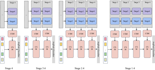
(a)

(b)

Figure 4: Assessing the impact of stage schemes on model performance.

These observations highlight the potential of HSQformer as a powerful tool in aiding clinical decision-making, particularly in high-stakes diagnostic contexts. The model’s ability to surpass the performance of less experienced clinicians and match that of seasoned experts suggests its utility in enhancing diagnostic accuracy and consistency. Furthermore, HSQformer’s robust performance in critical metrics such as Recall and AUC underscores its value in reducing missed diagnoses and improving patient outcomes.

4.3 Ablations

4.3.1 Macro Ablations

Stage Schemes.

In this section, we verify the macro design of HSQformer. As illustrated in Figure 4, we validate the effectiveness of the hierarchical design by incrementally incorporating CSM. Unless otherwise specified, all ablation study results are obtained on the multi-center test set, as this approach better validates the generalizability of the model. We observe a progressive increase in both F1 and AUC scores. Merely adding a CSM in the final stage results in a 1.77% improvement in F1 and a 0.43% enhancement in AUC compared to the baseline. The full-stage approach yields a 4.22% increase in F1 and a 0.76% improvement in AUC over the baseline.

Stage ratios.

Expanding on the findings depicted in Figure 4, this research delves into the influence exerted by the proportional parameters at various stages on the model’s performance. Employing state-of-the-art (SOTA) models as a reference point within the field[16, 53, 25, 56, 57], we conducted a comprehensive assessment of the model’s performance under multiple proportional settings, as elucidated in Figure 5. The results indicate that the HSQformer model demonstrates a negligible variation in performance with respect to different stage ratios, particularly with regard to the AUC, which shows a minimal trend of change. Despite this robustness, the experimental data has guided us in selecting the most effective ratio configuration, which is 2:2:6:2, to optimize the model’s performance.

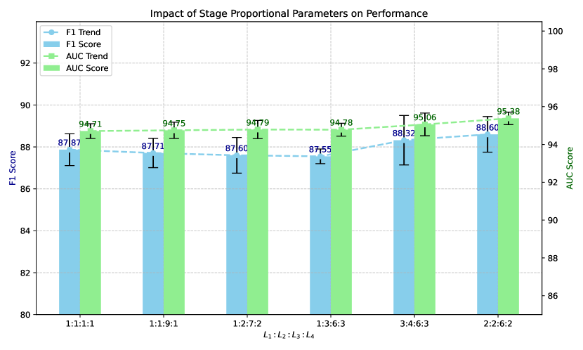
Figure 5: Influence of proportional parameters on model performance at different stages.

Query number and dimension.

Within the framework of model architecture, the parameters of Query number and dimension are crucial determinants of the model’s efficiency and efficacy. The Query number delineates the number of tokens the model queries during the information processing, signifying the model’s capability to manage a specific number of tokens in a single pass. The Query dimension, conversely, pertains to the dimension associated with these queries, which fundamentally establishes the capacity of each query to capture information. In the Figure 6, we meticulously examined the impact of query number and dimension on model performance. Specifically, when query quantity was held constant, incrementally increasing query dimension significantly enhanced the model’s F1 score and AUC. For instance, with a query number of 50, the F1 score improved from approximately 86.12% to about 87.17%, and the AUC score increased from approximately 94.04% to around 94.74% as the query dimension was augmented from 96 to 768. This suggests that a higher query dimension facilitates the model’s ability to capture long-range dependencies and subtle features, thereby enhancing classification performance.

Further analysis revealed that, with the query dimension held constant, a moderate increase in the number of queries significantly enhanced model performance. Specifically, at a query dimension of 768, the F1 score improved from approximately 87.13% to approximately 88.53%, and the AUC score increased from approximately 94.74% to approximately 95.09% as the number of queries increased from 50 to 100. However, when the number of queries was further increased to 300 and 400, the model performance, while remaining high, did not exhibit significant growth, a similar observation made at a dimension of 96. Moreover, concurrently increasing the number of queries and dimension can markedly improve model performance; for example, raising the number of queries and dimension from 50 and 96 to 400 and 768, respectively, resulted in an F1 score increase from approximately 86.12% to approximately 88.99%, and an AUC increase from approximately 94.04% to approximately 95.22%. Beyond a certain threshold, however, the performance enhancement plateaued, indicating the existence of an optimal balance point. It is important to highlight the trade-off between the number of queries and their dimension. Incrementing either parameter escalates computational costs and amplifies model complexity. Consequently, identifying the optimal equilibrium between these two parameters is pivotal for attaining superior performance while preserving computational efficiency.

4.3.2 Micro Ablations

Parallel and Serial Schemes.

This section primarily investigates the efficacy of the CSM at a micro-level design. We commence by examining the sequence of self-attention and cross-attention mechanisms, as depicted in Figure 7. Through our analysis, we ascertained that there is a negligible difference between the serial and parallel approaches. Nonetheless, we opted for the serial approach based on the hypothesis that query tokens initially capture relevant features through cross-attention, subsequently reinforcing these features via self-attention. This sequential methodology aligns with the design philosophy of the Transformer architecture, ensuring the rationality of our design.

Figure 6: Systematic analysis of query numbers and dimensions on model performance

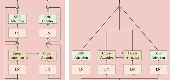
(a)

(b)

Figure 7: Serial vs. Parallel attention mechanisms: structural diagram and performance comparison.

MOE.

In the study of Mixture of Experts (MoE) models, the number of experts and the Top-K selection strategy employed by the router play a crucial role in determining model performance. In sparse MoE models, where the aim is to maintain computational efficiency, existing research predominantly adopts Top-1 or Top-2 selection strategies. This approach is taken because selecting more experts could undermine the sparsity advantage and increase computational overhead. Conversely, when all experts are activated irrespective of input, this dense configuration does not prioritize sparsity but instead focuses on leveraging the collective knowledge of all experts for potentially better performance. Figure 8 provides an insightful examination into the specific impacts of varying expert counts and routing strategies on model performance.When the number of experts is limited, MoE does not exhibit performance improvements over traditional MLP, which can be considered as having zero experts. Specifically, with only two experts and a Top-1 routing strategy, MoE achieves AUC (Area Under the Curve) scores that are comparable to those of MLP but does not show any significant improvement in F1 score; in fact, there is a decrease of 0.88% in the F1 score compared to the MLP. Furthermore, no substantial differences are observed between the Top-1 and Top-2 routing strategies under these conditions, indicating that a limited number of experts does not contribute to enhanced model performance. These results collectively suggest that when the number of experts is small($\leq 2$), MoE fails to provide performance benefits over conventional architectures like MLP, highlighting the necessity of increasing the number of experts or exploring alternative strategies to achieve superior performance in MoE. Building on this, as the number of experts in MoE increases to four or eight, significant performance improvements over MLPs are observed with a Top-1 routing strategy. The adoption of a Top-2 routing strategy further amplifies these performance benefits compared to the Top-1 approach. Interestingly, activating all experts in a dense MoE configuration does not lead to additional performance gains; instead, it may cause a slight decline, potentially due to the increased model complexity that could result in overfitting. Notably, under the Top-2 routing strategy, MoE with four and eight experts exhibit similar performance outcomes, indicating that four experts might provide an optimal balance between performance and efficiency. This insight is crucial for the design of efficient and high-performing MoE architectures.

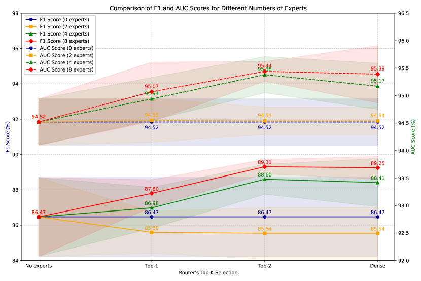
Figure 8: Trend curves of number of experts and Top-K selection strategy

5 Discussion and Limitations

Our research primarily focuses on evaluating the efficacy of AI technology in HCC screening, comparing its diagnostic performance against that of clinical radiologists. The results indicate that AI surpasses the diagnostic performance of junior radiologists and matches or even exceeds that of senior radiologists under certain conditions. This aligns with recent advancements in medical imaging analysis where AI has demonstrated significant improvements in both the speed and accuracy of diagnoses. By leveraging deep learning algorithms, AI models can analyze vast datasets of medical images to detect subtle patterns and features that may elude human observers, thereby aiding clinical decision-making. The designed AI model exhibited robust generalization capabilities across three distinct scenarios, underscoring its adaptability to variations in HCC imaging due to individual differences, tumor size, location, and growth rate. This consistency is particularly crucial for early-stage HCC screening as timely diagnosis plays a pivotal role in improving patient survival rates.However, while discussing the potential applications of AI in HCC diagnostics, it is imperative to acknowledge the challenges it faces in clinical practice. First, training and validating AI models require substantial amounts of high-quality data, which are time-consuming and costly to collect and annotate. Second, despite our provision of some visual insights into the model predictions, the interpretability of AI models remains an ongoing challenge, particularly when it comes to explaining the decision-making process to patients and healthcare providers.

While this study yields promising outcomes, several limitations must be addressed. The HSQformer, specifically tailored for ultrasonic HCC screening, incorporates hyperparameters such as query number and dimension, and the number of experts and Top-K selection strategy within the Mixture of Experts (MoE) framework. The applicability of these parameters to other domains requires further investigation. Additionally, our study emphasizes the efficacy of the model without delving into its parameter count. Although MoE enhances performance, it also substantially increases model size; however, only a subset of experts is activated during inference. Future work will explore the feasibility of using more compact models without compromising performance to enhance accessibility and broader application.

6 Conclusion

This study introduces an innovative Hierarchical Sparse Query Transformer model, designed to enhance the diagnostic accuracy of HCC ultrasound screening. By integrating the strengths of CNNs and ViTs, the HSQformer achieves superior performance across various clinical scenarios, including single-center, multi-center, and high-risk patient testing, significantly outperforming existing state-of-the-art models such as ConvNext and SwinTransformer. Furthermore, its diagnostic accuracy is comparable to that of senior radiologists and even surpasses junior radiologists in certain aspects. The HSQformer’s success underscores the immense potential of artificial intelligence in medical image analysis, particularly in improving diagnostic efficiency and accuracy. Its modular and extensible design philosophy ensures broad applicability and flexibility in real-world clinical settings. Additionally, the open-source code facilitates future research and development, contributing to the advancement of AI in the field of HCC screening.

Appendix

A Architecture Details

The HSQformer models (HSQformer-S, HSQformer-B, and HSQformer-L) are designed to scale in complexity and computational demand. The Small model offers a basic configuration, while the Base model enhances feature extraction. The Large model provides the most advanced capabilities, suitable for complex tasks. Table 4 summarizes their configurations.

Model	HSQformer-S	HSQformer-B	HSQformer-L
Query number	200	200	400
Query dimension	384	384	768
Stage ratio	1:1:1:1	2:2:6:2	2:2:6:2
MOE type	Sparse tokens	Sparse tokens	Sparse tokens
Number of experts	4	4	8
Top-K Strategy	Top-1	Top-2	Top-2
Input shape	Stage 1:$3136\times 384$ Stage 2:$784\times 384$ Stage 3:$196\times 384$ Stage 4:$48\times 384$	Stage 1:$3136\times 384$ Stage 2:$784\times 384$ Stage 3:$196\times 384$ Stage 4:$48\times 384$	Stage 1:$3136\times 768$ Stage 2:$784\times 768$ Stage 3:$196\times 768$ Stage 4:$48\times 768$
Output shape	$200\times 384$	$200\times 384$	$400\times 768$

Table 4: Configuration of Small, Base, and Large models.

B Training Settings

pre-training config[22, 16]	ImageNet-1K 2242
fine-tuning config	HSQformer-S/B/L
weight init	trunc. normal (0.2)
optimizer	AdamW
base learning rate	1e-4
weight decay	1e-4
optimizer momentum	$\beta_{1},\beta_{2}{=}0.9,0.999$
batch size	50(S-B)/20(L)
fine-tuning epochs	20
learning rate schedule	cosine decay
warmup epochs	1
warmup schedule	cosine
layer-wise lr decay	None
auto augment	IMAGENET
random resized crop	224/(0.7,1.0)
random horizontal flip	0.5
mixup	0.8
cutmix	1.0
random erasing	0.25
label smoothing	0.1
stochastic depth	0.2
dropout	0.5
layer scale	1e-6
head init scale	None
gradient clip	None
exp. mov. avg. (EMA)	None(S-B)/0.9999(L)

Table 5: Detailed overview of the training configurations.

Table 5 provides a detailed overview of the configurations used in both the pre-training and fine-tuning stages. The pre-training phase adheres to the protocol described in [18], with the primary objective of enabling the model to learn a robust set of features from a large-scale dataset. The fine-tuning stage builds upon the pre-trained model by adjusting various parameters to further enhance its performance, ensuring it is better suited to specific task requirements. This optimization strategy, transitioning from pre-training to fine-tuning, helps improve the model’s generalization and task adaptability.

C Visualization

In Figure 9, we conducted a systematic comparative analysis of the performance of state-of-the-art models on three different test datasets using a 5-fold cross-validation method. The figure provides an intuitive visualization of the models’ performance across various testing scenarios, thereby aiding in a deeper understanding of the strengths and limitations of each model. Figure 10, on the other hand, offers a hotspot analysis in the form of a heatmap. This heatmap visualization highlights the regions of interest in the ultrasound images where the models focus their attention for making predictions. The intensity of the colors in the heatmap corresponds to the importance of the respective regions, with brighter colors indicating higher significance. This interpretability analysis helps us understand the underlying patterns and features that the models rely on for diagnosing HCC, providing insights into their decision-making process.

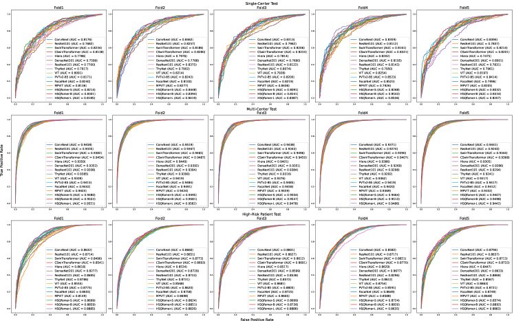
Figure 9: Systematic comparative analysis of SOTA models using 5-Fold cross-validation on three test datasets

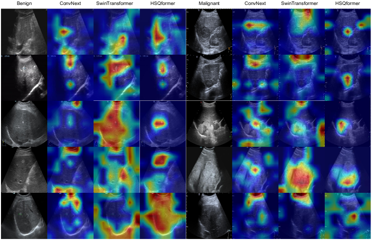
Figure 10: Heatmap analysis of attention maps for ultrasound HCC diagnosis.

References

- [1] F. Bray, M. Laversanne, H. Sung, J. Ferlay, R. L. Siegel, I. Soerjomataram, and A. Jemal, “Global cancer statistics 2022: Globocan estimates of incidence and mortality worldwide for 36 cancers in 185 countries,” CA: a cancer journal for clinicians, vol. 74, no. 3, pp. 229–263, 2024.
- [2] R. F. Hanna, V. Z. Miloushev, A. Tang, L. A. Finklestone, S. Z. Brejt, R. S. Sandhu, C. S. Santillan, T. Wolfson, A. Gamst, and C. B. Sirlin, “Comparative 13-year meta-analysis of the sensitivity and positive predictive value of ultrasound, ct, and mri for detecting hepatocellular carcinoma,” Abdominal radiology, vol. 41, pp. 71–90, 2016.
- [3] R. Chou, C. Cuevas, R. Fu, B. Devine, N. Wasson, A. Ginsburg, B. Zakher, M. Pappas, E. Graham, and S. D. Sullivan, “Imaging techniques for the diagnosis of hepatocellular carcinoma: a systematic review and meta-analysis,” Annals of internal medicine, vol. 162, no. 10, pp. 697–711, 2015.
- [4] A. Dosovitskiy, “An image is worth 16x16 words: Transformers for image recognition at scale,” arXiv preprint arXiv:2010.11929, 2020.
- [5] X. Ding, X. Zhang, J. Han, and G. Ding, “Scaling up your kernels to 31x31: Revisiting large kernel design in cnns,” in Proceedings of the IEEE/CVF conference on computer vision and pattern recognition, 2022, pp. 11 963–11 975.
- [6] S. Liu, T. Chen, X. Chen, X. Chen, Q. Xiao, B. Wu, T. Kärkkäinen, M. Pechenizkiy, D. Mocanu, and Z. Wang, “More convnets in the 2020s: Scaling up kernels beyond 51x51 using sparsity,” arXiv preprint arXiv:2207.03620, 2022.
- [7] H. Chen, X. Chu, Y. Ren, X. Zhao, and K. Huang, “Pelk: Parameter-efficient large kernel convnets with peripheral convolution,” in Proceedings of the IEEE/CVF Conference on Computer Vision and Pattern Recognition, 2024, pp. 5557–5567.
- [8] X. Ding, Y. Guo, G. Ding, and J. Han, “Acnet: Strengthening the kernel skeletons for powerful cnn via asymmetric convolution blocks,” in Proceedings of the IEEE/CVF international conference on computer vision, 2019, pp. 1911–1920.
- [9] X. Ding, X. Zhang, N. Ma, J. Han, G. Ding, and J. Sun, “Repvgg: Making vgg-style convnets great again,” in Proceedings of the IEEE/CVF conference on computer vision and pattern recognition, 2021, pp. 13 733–13 742.
- [10] A. Wang, H. Chen, Z. Lin, J. Han, and G. Ding, “Repvit: Revisiting mobile cnn from vit perspective,” in Proceedings of the IEEE/CVF Conference on Computer Vision and Pattern Recognition, 2024, pp. 15 909–15 920.
- [11] J. Dai, H. Qi, Y. Xiong, Y. Li, G. Zhang, H. Hu, and Y. Wei, “Deformable convolutional networks,” in Proceedings of the IEEE international conference on computer vision, 2017, pp. 764–773.
- [12] X. Zhu, H. Hu, S. Lin, and J. Dai, “Deformable convnets v2: More deformable, better results,” in Proceedings of the IEEE/CVF conference on computer vision and pattern recognition, 2019, pp. 9308–9316.
- [13] W. Wang, J. Dai, Z. Chen, Z. Huang, Z. Li, X. Zhu, X. Hu, T. Lu, L. Lu, H. Li et al., “Internimage: Exploring large-scale vision foundation models with deformable convolutions,” in Proceedings of the IEEE/CVF conference on computer vision and pattern recognition, 2023, pp. 14 408–14 419.
- [14] Y. LeCun, Y. Bengio et al., “Convolutional networks for images, speech, and time series,” The handbook of brain theory and neural networks, vol. 3361, no. 10, p. 1995, 1995.
- [15] Z. Lu, H. Xie, C. Liu, and Y. Zhang, “Bridging the gap between vision transformers and convolutional neural networks on small datasets,” Advances in Neural Information Processing Systems, vol. 35, pp. 14 663–14 677, 2022.
- [16] Z. Liu, Y. Lin, Y. Cao, H. Hu, Y. Wei, Z. Zhang, S. Lin, and B. Guo, “Swin transformer: Hierarchical vision transformer using shifted windows,” in Proceedings of the IEEE/CVF international conference on computer vision, 2021, pp. 10 012–10 022.
- [17] X. Pan, T. Ye, Z. Xia, S. Song, and G. Huang, “Slide-transformer: Hierarchical vision transformer with local self-attention,” in Proceedings of the IEEE/CVF conference on computer vision and pattern recognition, 2023, pp. 2082–2091.
- [18] X. Dong, J. Bao, D. Chen, W. Zhang, N. Yu, L. Yuan, D. Chen, and B. Guo, “Cswin transformer: A general vision transformer backbone with cross-shaped windows,” in Proceedings of the IEEE/CVF conference on computer vision and pattern recognition, 2022, pp. 12 124–12 134.
- [19] Y.-H. Wu, Y. Liu, X. Zhan, and M.-M. Cheng, “P2t: Pyramid pooling transformer for scene understanding,” IEEE transactions on pattern analysis and machine intelligence, vol. 45, no. 11, pp. 12 760–12 771, 2022.
- [20] W. Wang, E. Xie, X. Li, D.-P. Fan, K. Song, D. Liang, T. Lu, P. Luo, and L. Shao, “Pvt v2: Improved baselines with pyramid vision transformer,” Computational Visual Media, vol. 8, no. 3, pp. 415–424, 2022.
- [21] W. Yu, M. Luo, P. Zhou, C. Si, Y. Zhou, X. Wang, J. Feng, and S. Yan, “Metaformer is actually what you need for vision,” in Proceedings of the IEEE/CVF conference on computer vision and pattern recognition, 2022, pp. 10 819–10 829.
- [22] Z. Liu, H. Mao, C.-Y. Wu, C. Feichtenhofer, T. Darrell, and S. Xie, “A convnet for the 2020s,” in Proceedings of the IEEE/CVF conference on computer vision and pattern recognition, 2022, pp. 11 976–11 986.
- [23] H. Yunusa, S. Qin, A. H. A. Chukkol, A. A. Yusuf, I. Bello, and A. Lawan, “Exploring the synergies of hybrid cnns and vits architectures for computer vision: A survey,” arXiv preprint arXiv:2402.02941, 2024.
- [24] B. H. Ngo, N.-T. Do-Tran, T.-N. Nguyen, H.-G. Jeon, and T. J. Choi, “Learning cnn on vit: A hybrid model to explicitly class-specific boundaries for domain adaptation,” in Proceedings of the IEEE/CVF Conference on Computer Vision and Pattern Recognition, 2024, pp. 28 545–28 554.
- [25] K. He, X. Zhang, S. Ren, and J. Sun, “Deep residual learning for image recognition,” in Proceedings of the IEEE conference on computer vision and pattern recognition, 2016, pp. 770–778.
- [26] G. Huang, Z. Liu, L. Van Der Maaten, and K. Q. Weinberger, “Densely connected convolutional networks,” in Proceedings of the IEEE conference on computer vision and pattern recognition, 2017, pp. 4700–4708.
- [27] F. Yu, “Multi-scale context aggregation by dilated convolutions,” arXiv preprint arXiv:1511.07122, 2015.
- [28] J. Hu, L. Shen, and G. Sun, “Squeeze-and-excitation networks,” in Proceedings of the IEEE conference on computer vision and pattern recognition, 2018, pp. 7132–7141.
- [29] S. Woo, J. Park, J.-Y. Lee, and I. S. Kweon, “Cbam: Convolutional block attention module,” in Proceedings of the European conference on computer vision (ECCV), 2018, pp. 3–19.
- [30] A. Vaswani, “Attention is all you need,” Advances in Neural Information Processing Systems, 2017.
- [31] H. Wu, B. Xiao, N. Codella, M. Liu, X. Dai, L. Yuan, and L. Zhang, “Cvt: Introducing convolutions to vision transformers,” in Proceedings of the IEEE/CVF international conference on computer vision, 2021, pp. 22–31.
- [32] A. Hassani, S. Walton, N. Shah, A. Abuduweili, J. Li, and H. Shi, “Escaping the big data paradigm with compact transformers,” arXiv preprint arXiv:2104.05704, 2021.
- [33] J. Yang, C. Li, P. Zhang, X. Dai, B. Xiao, L. Yuan, and J. Gao, “Focal self-attention for local-global interactions in vision transformers,” arXiv preprint arXiv:2107.00641, 2021.
- [34] S. Mehta and M. Rastegari, “Mobilevit: light-weight, general-purpose, and mobile-friendly vision transformer,” arXiv preprint arXiv:2110.02178, 2021.
- [35] J. M. J. Valanarasu, P. Oza, I. Hacihaliloglu, and V. M. Patel, “Medical transformer: Gated axial-attention for medical image segmentation,” in Medical image computing and computer assisted intervention–MICCAI 2021: 24th international conference, Strasbourg, France, September 27–October 1, 2021, proceedings, part I 24. Springer, 2021, pp. 36–46.
- [36] A. Goyal, A. Didolkar, A. Lamb, K. Badola, N. R. Ke, N. Rahaman, J. Binas, C. Blundell, M. Mozer, and Y. Bengio, “Coordination among neural modules through a shared global workspace,” arXiv preprint arXiv:2103.01197, 2021.
- [37] J. Lee, Y. Lee, J. Kim, A. Kosiorek, S. Choi, and Y. W. Teh, “Set transformer: A framework for attention-based permutation-invariant neural networks,” in International conference on machine learning. PMLR, 2019, pp. 3744–3753.
- [38] A. Jaegle, S. Borgeaud, J.-B. Alayrac, C. Doersch, C. Ionescu, D. Ding, S. Koppula, D. Zoran, A. Brock, E. Shelhamer et al., “Perceiver io: A general architecture for structured inputs & outputs. arxiv, 2021,” arXiv preprint arXiv:2107.14795.
- [39] A. Jaegle, F. Gimeno, A. Brock, O. Vinyals, A. Zisserman, and J. Carreira, “Perceiver: General perception with iterative attention,” in International conference on machine learning. PMLR, 2021, pp. 4651–4664.
- [40] D. Li, J. Hu, C. Wang, X. Li, Q. She, L. Zhu, T. Zhang, and Q. Chen, “Involution: Inverting the inherence of convolution for visual recognition,” in Proceedings of the IEEE/CVF conference on computer vision and pattern recognition, 2021, pp. 12 321–12 330.
- [41] L. Yuan, Q. Hou, Z. Jiang, J. Feng, and S. Yan, “Volo: Vision outlooker for visual recognition,” IEEE transactions on pattern analysis and machine intelligence, vol. 45, no. 5, pp. 6575–6586, 2022.
- [42] M. Arar, A. Shamir, and A. H. Bermano, “Learned queries for efficient local attention,” in Proceedings of the IEEE/CVF Conference on Computer Vision and Pattern Recognition, 2022, pp. 10 841–10 852.
- [43] J. Ma, Z. Zhao, X. Yi, J. Chen, L. Hong, and E. H. Chi, “Modeling task relationships in multi-task learning with multi-gate mixture-of-experts,” in Proceedings of the 24th ACM SIGKDD international conference on knowledge discovery & data mining, 2018, pp. 1930–1939.
- [44] A. Yang, B. Yang, B. Zhang, B. Hui, B. Zheng, B. Yu, C. Li, D. Liu, F. Huang, H. Wei et al., “Qwen2. 5 technical report,” arXiv preprint arXiv:2412.15115, 2024.
- [45] D. Dai, C. Deng, C. Zhao, R. Xu, H. Gao, D. Chen, J. Li, W. Zeng, X. Yu, Y. Wu et al., “Deepseekmoe: Towards ultimate expert specialization in mixture-of-experts language models,” arXiv preprint arXiv:2401.06066, 2024.
- [46] A. Liu, B. Feng, B. Wang, B. Wang, B. Liu, C. Zhao, C. Dengr, C. Ruan, D. Dai, D. Guo et al., “Deepseek-v2: A strong, economical, and efficient mixture-of-experts language model,” arXiv preprint arXiv:2405.04434, 2024.
- [47] T. Zhu, X. Qu, D. Dong, J. Ruan, J. Tong, C. He, and Y. Cheng, “Llama-moe: Building mixture-of-experts from llama with continual pre-training,” in Proceedings of the 2024 Conference on Empirical Methods in Natural Language Processing, 2024, pp. 15 913–15 923.
- [48] X. Qu, D. Dong, X. Hu, T. Zhu, W. Sun, and Y. Cheng, “Llama-moe v2: Exploring sparsity of llama from perspective of mixture-of-experts with post-training,” arXiv preprint arXiv:2411.15708, 2024.
- [49] W. Cai, J. Jiang, F. Wang, J. Tang, S. Kim, and J. Huang, “A survey on mixture of experts,” arXiv preprint arXiv:2407.06204, 2024.
- [50] K. He, X. Chen, S. Xie, Y. Li, P. Dollár, and R. Girshick, “Masked autoencoders are scalable vision learners,” in Proceedings of the IEEE/CVF conference on computer vision and pattern recognition, 2022, pp. 16 000–16 009.
- [51] S. Xie, R. Girshick, P. Dollár, Z. Tu, and K. He, “Aggregated residual transformations for deep neural networks,” in Proceedings of the IEEE conference on computer vision and pattern recognition, 2017, pp. 1492–1500.
- [52] S. Peng, Y. Liu, W. Lv, L. Liu, Q. Zhou, H. Yang, J. Ren, G. Liu, X. Wang, X. Zhang et al., “Deep learning-based artificial intelligence model to assist thyroid nodule diagnosis and management: a multicentre diagnostic study,” The Lancet Digital Health, vol. 3, no. 4, pp. e250–e259, 2021.
- [53] C. Ryali, Y.-T. Hu, D. Bolya, C. Wei, H. Fan, P.-Y. Huang, V. Aggarwal, A. Chowdhury, O. Poursaeed, J. Hoffman et al., “Hiera: A hierarchical vision transformer without the bells-and-whistles,” in International Conference on Machine Learning. PMLR, 2023, pp. 29 441–29 454.
- [54] J. Yang, C. Li, X. Dai, and J. Gao, “Focal modulation networks,” Advances in Neural Information Processing Systems, vol. 35, pp. 4203–4217, 2022.
- [55] A. Farhadi and J. Redmon, “Yolov3: An incremental improvement,” in Computer vision and pattern recognition, vol. 1804. Springer Berlin/Heidelberg, Germany, 2018, pp. 1–6.
- [56] Y. Lee, J. Kim, J. Willette, and S. J. Hwang, “Mpvit: Multi-path vision transformer for dense prediction,” in Proceedings of the IEEE/CVF conference on computer vision and pattern recognition, 2022, pp. 7287–7296.
- [57] M. Ding, B. Xiao, N. Codella, P. Luo, J. Wang, and L. Yuan, “Davit: Dual attention vision transformers,” in European conference on computer vision. Springer, 2022, pp. 74–92.