Logarithmic fluctuations of Stationary Hastings-Levitov

Noam Berger Department of mathematics, TUM https://www.math.cit.tum.de/en/probability/people/berger/ noam.berger@tum.de  and  Eviatar B. Procaccia Technion - Israel Institute of Technology http://procaccia.net.technion.ac.il eviatarp@technion.ac.il
Abstract.

We prove that the fluctuation field $\{M_{t}(x)\}_{x\in{\mathbb{R}}}$ of stationary Hastings-Levitov$(0)$ exhibits logarithmic spatial correlations. Moreover, by studying the infinitesimal generator of the imaginary part of $M_{t}(0)$, we show that for some $\beta>0$, $\max_{x\in[0,t]}\text{Im}M_{t}(x)<\beta\log t$ with high probability, as $t\to\infty$.

1. Introduction

Stationary Hastings-Levitov$(0)$ (SHL$(0)$) was introduced and studied by the authors with Turner as a stationary off-lattice version of Diffusion Limited Aggregation defined as the composition of conformal slit maps from the upper half complex plane. Unlike the classical Hastings-Levitov process on the complement of the unit disk [HL98, NT12, Sil17], where slit normalization is required to avoid blowup, in the half plane geometry un-normalized particle sizes remain tight. Using this simplicity, it is shown in [BPT22] that the harmonic measure of an interval is a martingale that scales to 0 like the distance of two brownian motions starting at the interval’s end points. It follows that at time $t>0$, the typical trees in the aggregate reach a height of $\frac{\pi}{2}t$ and contain an order of $t^{3/2}$ particles. This matches a prediction by Meakin [Mea83] and was verified in computer simulations [PP21] for DLA grown on the half plane (the so called Stationary DLA [PZ19, PYZ20, MPZ22]). Other stationary versions of aggregation processes where studied, and all share some universal geometric attributes such as finiteness of all trees a.s at time $\infty$ [BKP14, AP17].

The SHL$(0)$ is defined by the following procedure: considering an intensity $1$ Poisson point process $\mathfs{A}$ on ${\mathbb{R}}\times{\mathbb{R}}_{+}$, and order $\mathfs{A}\cap([-m,m]\times{\mathbb{R}}_{+}):=\{(x_{1},t_{1}),(x_{2},t_{2}),\ldots\}$ by the second coordinate (arrival times). Define for any $z\in{\mathbb{H}}=\{z\in{\mathbb{C}}:\text{Im}z>0\}$,

(1) $\displaystyle\tilde{F}_{t}^{m}(z)=\left\{\begin{array}[]{ll}0&t<t_{1}\\ \varphi_{x_{1}}\circ\varphi_{x_{2}}\circ\cdots\circ\varphi_{x_{k}}(z)&t_{k}\leq t<t_{k+1}\end{array}\right.,$

with the slit map $\varphi_{x}(z)=x+\sqrt{(z-x)^{2}-1}$, using the branch of $\sqrt{\cdot}$ for which the imaginary part is positive. The SHL$(0)$ is defined by taking the limit $\tilde{F}_{t}(z)=\lim_{m\to\infty}\tilde{F}_{t}^{m}(z)$.

Refer to caption
Figure 1. Computer simulation of $\{\tilde{F}_{t}(x)\}_{x\in{\mathbb{R}}}$

Note that for any $t$, $\tilde{F}^{m}_{t}$ has the same distribution as

(2) $\displaystyle{F}_{t}^{m}(z)=\left\{\begin{array}[]{ll}0&t<t_{1}\\ \varphi_{x_{k}}\circ\varphi_{x_{k-1}}\circ\cdots\circ\varphi_{x_{1}}(z)&t_{k}\leq t<t_{k+1}\end{array}\right.,$

and by taking the limit we obtain the backwards SHL$(0)$, $F_{t}(z)=\lim_{m\to\infty}F_{t}^{m}(z)$. It is shown in [BPT22] that one can write

(3) $\displaystyle F_{t}(z)=z+it\frac{\pi}{2}+M_{t}(z),$

where $M_{t}(z)$ is a zero mean martingale, which can be realized as the limit of the martingale part in the Doob decomposition

(4) $$F^{m}_{t}(z)=z+D^{m}_{t}(z)+M^{m}_{t}(z).$$

In this paper we study the field $\{M_{t}(x)\}_{x\in{\mathbb{R}}}$ and prove it observes logarithmic spatial correlation and study the maximum of the field.

Refer to caption
Figure 2. Computer simulation of $\{M_{t}(x)\}_{x\in{\mathbb{R}}}$

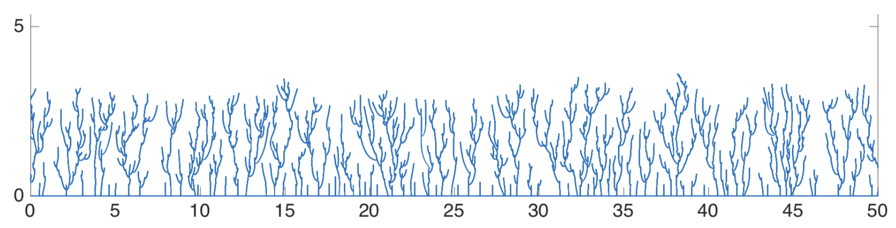
Logarithmic correlation for the small particle limit of the original Hastings-Levitov $(0)$ process were discovered by Silvestri in [Sil17]. We propose a distinct approach compared to Silvestri’s, focusing on the physical process rather than its scaling limit. Specifically, we demonstrate the logarithmic correlations of fluctuations for the SHL(0) process itself. Note that by computer simulations (see Figure 2), without considering the scaling limit, it doesn’t appear that the field $\{M_{t}(x)\}_{x\in{\mathbb{R}}}$ is Gaussian. See Figure 3 for a simulated histogram of the marginal distribution, note the lack of symmetry.

Refer to caption
Figure 3. $M_{t}(0)$ empirical distribution histogram

1.1. Results

First we improve the diffusive bound proved in [BPT22].

Theorem 1.

As $t\to\infty$, $\mathbf{E}[|M_{t}(0)|^{2}]=\frac{\pi}{4}\log t(1+o(1)).$

Next we claim that $\{M_{t}(x)\}_{x}$ admits logarithmic correlations.

Theorem 2.
$$\mathrm{Cov}(M_{t}(0),M_{t}(b))=\frac{\pi}{4}\min\{\log(t)-\log(b),0\}(1+o(1)),$$

where the little $o$ notation is with respect to $b\to\infty$.

Lastly for the behavior maximum of the field, let

(5) $\displaystyle\mathfs{M}_{t}=\max_{x\in[0,t]}\text{Im}M_{t}(x).$
Theorem 3.

There exists a $c>0$ such that for any $\beta>0$ large enough, for every $t>0$ large enough,

(6) $\displaystyle{\bf P}\left(\max_{x\in[0,t]}\text{Im}M_{t}(x)>\beta\log t\right)<\frac{c}{t^{1/2}}.$

2. Proof of Theorem 1

First we improve the law of large numbers estimate from [BPT22].

Lemma 2.1.

There exist ξ2.1,c2.1>0\xi_{\ref{lem:llnrate}},c_{\ref{lem:llnrate}}>0 such that for every $z\in{\mathbb{H}}$,

𝐏[ImFt(z)<Imz+ξ2.1t]<ec2.1t.{\bf P}\left[\text{Im}F_{t}(z)<\text{Im}z+\xi_{\ref{lem:llnrate}}t\right]<e^{-c_{\ref{lem:llnrate}}t}.
Proof.

W.l.o.g we assume that $\frac{t}{m}\in{\mathbb{N}}$, for some $m$ that will be chosen later, and we write

$$F_{t}(z)=G_{t/m}\circ G_{t/m-1}\circ\cdots\circ G_{1}(z),$$

where the $G_{i}$ are i.i.d. and distributed as $F_{m}$. By [BPT22, Lemma 5.1] we obtain that there are $M_{m}^{i}$ i.i.d with mean zero such that $G_{i}(z)=z+i\frac{m\pi}{2}+M_{m}^{i}$. Moreover,

(7) $${\bf P}\left[\text{Im}G_{1}(z)>\text{Im}z+\frac{m\pi}{4}\right]\geq 1-{\bf P}\left[|M_{1}(z)|>\frac{m\pi}{4}\right]\geq 1-\frac{c}{(1+\text{Im}z)m}.$$

Thus, for $m$ large enough, there is a $\xi>0$ such that for any $z\in{\mathbb{H}}$,

(8) $\displaystyle{\bf P}\left[\text{Im}G_{1}(z)>\text{Im}z+\frac{m\pi}{4}\right]\geq\xi.$

Since $G_{i}$ are independent, we obtain that

(9) $\displaystyle{\bf P}\left[\text{Im}M_{i}(G_{i-1}\circ G_{i-2}\circ\cdots\circ G_{1}(z))>-\frac{m\pi}{4}\right]\geq\xi.$

Denote $N_{t}=|\{i\leq t/m:\text{Im}M_{i}(G_{i-1}\circ G_{i-2}\circ\cdots\circ G_{1}(z))>-\frac{m\pi}{4}\}|$. By Hoeffding’s inequality there is a $\zeta>0$ such that,

(10) $\displaystyle{\bf P}\left(N_{t}<\frac{\xi}{2}t/m\right)<\zeta^{t/m}.$

Under the event $\left\{N_{t}\geq\frac{\xi}{2}t/m\right\}$, we obtain $F_{t}(z)\geq\frac{\pi}{4}\frac{\xi}{2}t$. By choosing ξ2.1=π2ξ2\xi_{\ref{lem:llnrate}}=\frac{\pi}{2}\frac{\xi}{2} we obtain for some c2.1>0c_{\ref{lem:llnrate}}>0 that

𝐏[ImFt(z)<Imz+ξ2.1t]<ec2.1t.{\bf P}\left[\text{Im}F_{t}(z)<\text{Im}z+\xi_{\ref{lem:llnrate}}t\right]<e^{-c_{\ref{lem:llnrate}}t}.

With Lemma 2.1, we are ready to prove Theorem 1. The proof employs a bootstrapping approach, iteratively refining fluctuation bounds and incorporating them back into the martingale representation.

Proof of Theorem 1.

We first condition on the likely event

$$H_{1}(\eta)=\left\{\forall s>\eta:\text{Im}F_{s}(0)>\frac{s}{\log(s^{\alpha})}\right\},$$

then bound the fluctuations, in order to guarantee that the event

$$H_{2}(s)=\left\{\text{Im}F_{s}(0)>\pi s/2-s^{2/3}\right\}$$

is highly likely. By Lemma 2.1, there exists a $c>0$ such that for $\alpha$ large enough, that will be chosen later,

$${\bf P}[H_{1}(\eta)]>1-\frac{c}{\eta^{c\alpha-1}}.$$

By (3) and [BPT22, Lemma 3.3] we write,

(11) $\displaystyle\mathbf{E}\left[|M_{t}(0)|^{2}\right]$ $\displaystyle=\mathbf{E}\left[\int_{0}^{t}\int_{-\infty}^{\infty}\Big{|}\varphi_{x}(F_{s}(0))-F_{s}(0)\Big{|}^{2}dxds\right]\leq\mathbf{E}\left[\int_{0}^{t}\frac{c}{1+\text{Im}F_{s}(0)}ds\right]$
$\displaystyle=\mathbf{E}\left[\int_{0}^{\eta}\frac{c}{1+\text{Im}F_{s}(0)}ds\right]+\mathbf{E}\left[\int_{\eta}^{t}\frac{c}{1+\text{Im}F_{s}(0)}\left({\mathbbm{1}}_{H_{1}(\eta)}+{\mathbbm{1}}_{H_{1}(\eta)^{c}}\right)ds\right]$
$\displaystyle\leq c\eta+\mathbf{E}\left[\int_{\eta}^{t}\frac{c}{1+\text{Im}F_{s}(0)}ds{\mathbbm{1}}_{H_{1}(\eta)}\right]+ct\eta^{1-c\alpha}$
$\displaystyle\leq c\eta+c\int_{\eta}^{t}\frac{\log s}{s}+ct\eta^{1-c\alpha}=c\eta+ct\eta^{1-c\alpha}+c(\log t)^{2}-c(\log\eta)^{2}$

Now take $\eta=t^{\beta}$ for $\beta=\frac{1}{6}$ and choosing $\alpha>\frac{1}{c\beta}$ , to obtain

$$\mathbf{E}\left[|M_{t}(0)|^{2}\right]\leq ct^{\beta}(1+o(1)).$$

We thus obtain that

$${\bf P}\left[\text{Im}F_{t}(0)<\frac{\pi t}{2}-t^{\gamma}\right]\leq{\bf P}\left[|M_{t}(0)|>t^{\gamma}\right]\leq\frac{t^{\beta}}{t^{2\gamma}}.$$

Choosing $\gamma=\frac{2}{3}$ yields the bound

$${\bf P}[H_{2}(s)]>1-\frac{c}{s^{1+1/6}}.$$

Repeating the earlier argument with $H_{2}(\eta)$ replacing $H_{1}(\eta)$ and using the quantitative Lemma A.1,

(12) $\displaystyle\mathbf{E}\left[|M_{t}(0)|^{2}\right]$ $\displaystyle\leq\mathbf{E}\left[\int_{0}^{t}\min\left\{1,\frac{\pi}{4\text{Im}F_{s}(0)}+\frac{c}{(\text{Im}F_{s}(0))^{3}}\right\}({\mathbbm{1}}_{H_{2}(s)}+{\mathbbm{1}}_{H^{c}_{2}(s)})ds\right]$
$\displaystyle\leq 1+\int_{1}^{t}\Bigg{(}\frac{\pi}{4s}+\frac{c}{s^{3}}+\frac{c}{s^{1+1/6}}\Bigg{)}ds.$

We conclude that

$$\mathbf{E}[|M_{t}(0)|^{2}]\leq\frac{\pi}{4}\log t(1+o(1)),$$

proving the upper bound.

As for the lower bound, define

(13) $\displaystyle H^{\prime}_{2}(\eta)=\left\{\forall\eta<s:\text{Im}F_{s}(0)>\pi s/2-s^{2/3}\right\}$
$\displaystyle H_{3}(\eta)=\left\{\forall\eta<s:\text{Im}F_{s}(0)<\pi s/2+s^{2/3}\right\}$
$\displaystyle H_{4}(\eta)=H_{3}(\eta)\cap H^{\prime}_{2}(\eta).$

Hence, for $\eta$ large enough, by Lemma A.1,

(14) $\displaystyle\mathbf{E}\left[|M_{t}(0)|^{2}\right]$ $\displaystyle\geq\mathbf{E}\left[\int_{0}^{t}\int_{-\infty}^{\infty}\Big{|}\varphi_{x}(F_{s}(0))-F_{s}(0)\Big{|}^{2}dxds{\mathbbm{1}}_{H_{4}(\eta)}\right]$
$\displaystyle\geq\mathbf{E}\left[\int_{\eta}^{t}\min\left\{1,\frac{\pi}{4\text{Im}F_{s}(0)}-\frac{c}{(\text{Im}F_{s}(0))^{3}}\right\}ds{\mathbbm{1}}_{H_{4}(\eta)}\right]$
$\displaystyle\geq\frac{\pi}{4}{\bf P}[H_{4}(\eta)]\int_{\eta}^{t}\frac{1}{s}=\frac{\pi}{4}(1-\eta^{-1/3})\left[\log t-\log\eta-o\left(\eta^{-1}\right)\right],$

Now taking $\eta=\sqrt{t}$, we obtain the lower bound for the variance. ∎

3. Proof of Theorem 2

We prove Theorem 2 by a sequence of lemmas dealing with different regimes of $t$ and $b$. Before continuing, we will bootstrap the earlier results to improve the fluctuation estimate of Lemma 2.1.

Lemma 3.1.

For any $z\in{\mathbb{H}}$,

𝐏(ImFt(z)<π2tt)<ec3.1t16.{\bf P}\left(\text{Im}F_{t}(z)<\frac{\pi}{2}t-\sqrt{t}\right)<e^{-c_{\ref{lem:bootstrapfluctuationrate}}t^{\frac{1}{6}}}.
Proof.

Let $G_{t^{\alpha}}^{j}(z)=z+i\frac{\pi}{2}t^{\alpha}+M_{t^{\alpha}}^{j}(z)$ be i.i.d. distributed as $F_{t^{\alpha}}(z)$. By Theorem 1, for any $z\in{\mathbb{H}}$,

(15) $\displaystyle{\bf P}\left(|M_{t^{\alpha}}^{j}(z)|>t^{\beta}\right)\leq\frac{c\alpha\log t}{t^{2\beta}}.$

Denote $N_{t}=\left|\{1\leq j\leq t^{1-\alpha}:|M_{t^{\alpha}}^{j}(G_{t^{\alpha}}^{j-1}\circ\cdots\circ G_{t^{\alpha}}^{1}(z))|<t^{\beta}\}\right|$. By Hoeffding’s inequality

(16) $\displaystyle{\bf P}\left(N_{t}<\left(1-\frac{2c\alpha\log t}{t^{2\beta}}\right)t^{1-\alpha}\right)<e^{ct^{1-\alpha}}$

Thus, on an event with probability greater than $1-e^{ct^{1-\alpha}}$, we get that

(17) $\displaystyle\text{Im}F_{t}(z)$ $\displaystyle\geq\left(1-\frac{2c\alpha\log t}{t^{2\beta}}\right)t^{1-\alpha}\left(\frac{\pi}{2}t^{\alpha}-t^{\beta}\right)=\left(1-\frac{2c\alpha\log t}{t^{2\beta}}\right)\left(\frac{\pi}{2}t-t^{1-\alpha+\beta}\right)$
$\displaystyle\geq\frac{\pi}{2}t-t^{1-\alpha+\beta}-2c\alpha\log t\frac{\pi}{2}t^{1-2\beta}.$

Choose $\alpha=\frac{5}{6}$ and $\beta=\frac{1}{3}$ to obtain the statement for some constant c3.1>0c_{\ref{lem:bootstrapfluctuationrate}}>0. ∎

Next, we prove that in order to study the fluctuations of $F_{t}$ it is enough to grow the process on a window of size $f(t)$, which depends on $t$ in a way which we describe below. Remember the definition of $M_{t}^{m}(z)$ from (4).

Lemma 3.2.

There is a $c>0$ such that for any function $f(t)$ satisfying $\lim_{t\to\infty}\frac{t}{f(t)}=0$, for any $t$ large enough,

(18) $\displaystyle\mathbf{E}\left[\Big{|}M_{t}(0)-M_{t}^{f(t)}(0)\Big{|}^{2}\right]<\frac{ct}{f(t)}.$
Proof.

Since both $M_{s}(0)$ and $M_{s}^{f(s)}(0)$ are zero mean martingales, so is their difference. Thus we can write

(19) $\displaystyle\mathbf{E}\left[\Big{|}M_{t}(0)-M_{t}^{f(t)}(0)\Big{|}^{2}\right]$ $\displaystyle\leq 8\mathbf{E}\left[\int_{0}^{t}\int_{-f(t)}^{f(t)}\Big{|}(\varphi_{x}-\text{id})F_{s}(0)-(\varphi_{x}-\text{id})F_{s}^{f(t)}(0)\Big{|}^{2}dxds\right]$
$\displaystyle+8\mathbf{E}\left[\int_{0}^{t}\int_{|x|>f(t)}\Big{|}\varphi_{x}(F_{s}(0))-F_{s}(0)\Big{|}^{2}dxds\right].$

By [BPT22, Lemma 3.3] we have that for all $x>2$,

$$\Big{|}\varphi_{x}(F_{s}(0))-F_{s}(0)\Big{|}^{2}\leq\frac{c}{x^{2}+(\text{Im}F_{s}(0))^{2}}.$$

Thus,

(20) $\displaystyle\mathbf{E}\left[\int_{0}^{t}\int_{|x|>f(t)}\Big{|}\varphi_{x}(F_{s}(0))-F_{s}(0)\Big{|}^{2}dxds\right]$
$\displaystyle\leq\mathbf{E}\left[\int_{0}^{t}\frac{2}{\text{Im}F_{s}(0)}\left[\frac{\pi}{2}-\tan^{-1}\left(\frac{f(t)}{\text{Im}F_{s}(0)}\right)\right]ds\right]\leq\frac{2t}{f(t)}.$

As for the other summand of (19), We take a path $\gamma^{s}:[0,1]\to{\mathbb{C}}$ connecting $F_{s}(0)$ and $F_{s}^{f(t)}$ and write

(21) $\displaystyle\Big{|}(\varphi_{x}-\text{id})F_{s}(0)-(\varphi_{x}-\text{id})F_{s}^{f(t)}(0)\Big{|}^{2}\leq|F_{s}(0)-F_{s}^{f(t)}(0)|^{2}\int_{0}^{1}\Big{|}\varphi^{\prime}_{x}(\gamma^{s}(u))-1\Big{|}^{2}du$

Denote $g(t)=\mathbf{E}\left[\max_{s\leq t}\Big{|}F_{s}(0)-F_{s}^{f(s)}(0)\Big{|}^{2}\right]$, and the event H3.1(s)={ImFs(z)π2ss}H_{\ref{lem:bootstrapfluctuationrate}}(s)=\{\text{Im}F_{s}(z)\geq\frac{\pi}{2}s-\sqrt{s}\}, thus

(22) $\displaystyle\mathbf{E}\left[\int_{0}^{t}\int_{-\infty}^{\infty}\Big{|}(\varphi_{x}-\text{id})F_{s}(0)-(\varphi_{x}-\text{id})F_{s}^{f(t)}(0)\Big{|}^{2}dxds\right]$
c0t𝐏(H3.1(s)c)+𝐄[0t|(φxid)Fs(0)(φxid)Fsf(t)(0)|2𝑑x𝑑s𝟙H3.1(s)]\displaystyle\leq c\int_{0}^{t}{\bf P}(H_{\ref{lem:bootstrapfluctuationrate}}(s)^{c})+\mathbf{E}\left[\int_{0}^{t}\int_{-\infty}^{\infty}\Big{|}(\varphi_{x}-\text{id})F_{s}(0)-(\varphi_{x}-\text{id})F_{s}^{f(t)}(0)\Big{|}^{2}dxds{\mathbbm{1}}_{H_{\ref{lem:bootstrapfluctuationrate}}(s)}\right]
c+𝐄[0tmaxst|Fs(0)Fsf(s)(0)|2c1+Im(Fs(0))3ds𝟙H3.1(s)]\displaystyle\leq c+\mathbf{E}\left[\int_{0}^{t}\max_{s\leq t}\Big{|}F_{s}(0)-F_{s}^{f(s)}(0)\Big{|}^{2}\frac{c}{1+\text{Im}(F_{s}(0))^{3}}ds{\mathbbm{1}}_{H_{\ref{lem:bootstrapfluctuationrate}}(s)}\right]
$\displaystyle\leq c+\int_{0}^{t}g(s)\frac{c}{1+s^{3}}ds,$

where in the first inequality we used the fact that there is a $c>0$ such that $|\varphi_{x}(z)-z|<c$ for all $x\in{\mathbb{R}}$ and $z\in{\mathbb{H}}$ (see [BPT22, Appendix A]). Now by Gronwall’s inequality, for some sonstant $c>0$,

(23) $\displaystyle g(t)\leq\frac{2t}{f(t)}e^{c},$

Finishing the proof.

Lemma 3.3.

For any $t>0$ and and $b\geq 2t\log(t)^{3}$, we have

$$\Big{|}\mathrm{Cov}(M_{t}(0),M_{t}(b))\Big{|}\leq c\sqrt{\frac{t}{b}\log t}.$$
Proof.
(24) $\displaystyle\mathbf{E}[M_{t}(0)M_{t}(b)]$
$\displaystyle=\mathbf{E}\Big{[}(M_{t}(0)-M_{t}^{f(t)}(0)+M_{t}^{f(t)}(0))(M_{t}(b)-M_{t}^{f(t)}(b)+M_{t}^{f(t)}(b))\Big{]}$
$\displaystyle=\mathbf{E}\Big{[}(M_{t}(0)-M_{t}^{f(t)}(0))M_{t}^{f(t)}(b)\Big{]}+\mathbf{E}\Big{[}(M_{t}(b)-M_{t}^{f(t)}(b))M_{t}^{f(t)}(0)\Big{]}$
$\displaystyle+\mathbf{E}\Big{[}(M_{t}(0)-M_{t}^{f(t)}(0))(M_{t}(b)-M_{t}^{f(t)}(b))\Big{]}+\mathbf{E}[M_{t}^{f(t)}(0)M_{t}^{f(t)}(b)]$

By applying Cauchy-Schwartz and Lemma 3.2 with the choice $f(t)=b/2>t\log(t)^{3}$, and the fact that $M_{t}^{f(t)}(0)$ and $M_{t}^{f(t)}(b)$ are independent, we obtain

(25) $\displaystyle\Big{|}\mathbf{E}[M_{t}(0)M_{t}(b)]\Big{|}\leq 2\sqrt{\frac{ct}{f(t)}\log t}+\frac{ct}{f(t)}+0$

Thus by our choice of $f(t)$ then the RHS of (LABEL:eq:covzerorate) is smaller than $c\sqrt{\frac{t}{b}\log t}$. ∎

Lemma 3.4.

For any $t>b$, we have

$$\Big{|}\mathrm{Cov}(M_{t}(0),M_{t}(b))\Big{|}=\frac{\pi}{4}\Big{(}\log(t)-\log(b)\Big{)}+O\Big{(}\log\log(b)+\sqrt{\log\log(b)}\sqrt{\log b}\Big{)},$$

as $b\to\infty$.

Proof.

First we bound using Lemma 3.3,

(26) $\displaystyle\mathbf{E}\Big{[}(M_{b/\log(b)^{3}}(b)-M_{0}(b))(M_{b/\log(b)^{3}}(0)-M_{0}(0))\Big{]}$ $\displaystyle=\mathbf{E}\Big{[}M_{b/\log(b)^{3}}(b)M_{b/\log(b)^{3}}(0)\Big{]}$
$\displaystyle\leq\frac{1}{\log{(b/\log{(b)^{3}}})}$

Second by the martingale property for $t>s$,

$$\mathbf{E}[|M_{t}(b)-M_{s}(b)|^{2}]=\mathbf{E}[|M_{t}(b)|^{2}-|M_{s}(b)|^{2}],$$

so by Theorem 1

(27) $\displaystyle\mathbf{E}\Big{[}(M_{b\log(b)^{3}}(b)-M_{b/\log(b)^{3}}(b))M_{t}(0)\Big{]}$
$\displaystyle=\mathbf{E}\Big{[}(M_{b\log(b)^{3}}(b)-M_{b/\log(b)^{3}}(b))(M_{t}(0)-M_{b\log(b)^{3}}(0)+M_{b\log(b)^{3}}(0))\Big{]}$
$\displaystyle=\mathbf{E}\Big{[}(M_{b\log(b)^{3}}(b)-M_{b/\log(b)^{3}}(b))M_{b\log(b)^{3}}(0)\Big{]}$
$\displaystyle\leq\sqrt{\mathbf{E}\Big{[}\Big{|}(M_{b\log(b)^{3}}(b)-M_{b/\log(b)^{3}}(b))\Big{|}^{2}\Big{]}\mathbf{E}\Big{[}\Big{|}(M_{b\log(b)^{3}}(0)\Big{|}^{2}\Big{]}}$
$\displaystyle\leq c\sqrt{\log({b\log(b)^{3})}}\Big{(}\sqrt{\log(b\log(b)^{3})-log(b/\log(b)^{3})}\Big{)}\leq c\sqrt{\log\log(b)^{3}}\sqrt{\log b},$

where in the second equality we used the martingale property and the fact that $M_{s}(b)$ and $M_{s}(0)$ are martingales on a common filtration i.e. for $t_{1}<t_{2}<t_{3}$, $\mathbf{E}\left[(M_{t_{2}}(b)-M_{t_{1}}(b))(M_{t_{3}}(0)-M_{t_{2}}(0))\right]=0$.

The third and final estimate we need before we can complete the proof of the lemma follows Cauchy-Schwarz and (12),

(28) $\displaystyle\left|\mathbf{E}\Big{[}(M_{t}(b)-M_{b\log(b)^{3}}(b))(M_{t}(0)-M_{b\log(b)^{3}}(0))\Big{]}\right|$
$\displaystyle\leq\sqrt{\mathbf{E}\Big{[}|M_{t}(b)-M_{b\log(b)^{3}}(b)|^{2}\Big{]}}\sqrt{\mathbf{E}\Big{[}|M_{t}(0)-M_{b\log(b)^{3}}(0)|^{2}\Big{]}}$
$\displaystyle\leq\frac{\pi}{4}\Big{(}\log(t)-\log(b\log(b)^{3})\Big{)}.$

Finally we can estimate using (26), (LABEL:eq:2bound), (LABEL:eq:1bound),

(29) $\displaystyle\Big{|}\mathrm{Cov}(M_{t}(0),M_{t}(b))\Big{|}=$
$\displaystyle\Big{|}\mathbf{E}\Big{[}\Big{(}(M_{t}(b)-M_{b\log(b)^{3}}(b))+(M_{b\log(b)^{3}}(b)-M_{b/\log(b)^{3}}(b))+(M_{b/\log(b)^{3}}(b)-M_{0}(b))\Big{)}$
$\displaystyle\Big{(}(M_{t}(0)-M_{b\log(b)^{3}}(0))+(M_{b\log(b)^{3}}(0)-M_{b/\log(b)^{3}}(0))+(M_{b/\log(b)^{3}}(0)-M_{0}(0))\Big{)}\Big{]}\Big{|}$
$\displaystyle\leq\frac{\pi}{4}\Big{(}\log(t)-\log(b)\Big{)}+O(\log(\log(b))+\sqrt{\log\log(b)}\sqrt{\log b}).$

For the lower bound we write from the first line of (LABEL:eq:1bound),

(30) $\displaystyle\mathbf{E}\Big{[}(M_{t}(b)-M_{b\log(b)^{3}}(b))(M_{t}(0)-M_{b\log(b)^{3}}(0))\Big{]}=$
$\displaystyle\mathbf{E}\Big{[}(M_{t}(b)-M_{b\log(b)^{3}}(b))^{2}$
$\displaystyle+(M_{t}(b)-M_{b\log(b)^{3}}(b))(M_{t}(0)-M_{b\log(b)^{3}}(0)-M_{t}(b)+M_{b\log(b)^{3}}(b))\Big{]}$

Note that for $r<t$

(31) $\displaystyle\mathbf{E}\left[|M_{t}(0)-M_{t}(b)|^{2}-|M_{r}(0)-M_{r}(b)|^{2}\right]$
$\displaystyle=\mathbf{E}\left[\int_{r}^{t}\int_{-\infty}^{\infty}\Big{|}(\varphi_{x}-\text{id})F_{s}(0)-(\varphi_{x}-\text{id})F_{s}(b)\Big{|}^{2}dxds\right]$
$\displaystyle\leq\mathbf{E}\left[\int_{r}^{t}\int_{-\infty}^{\infty}\Big{(}|F_{s}(0)-F_{s}(b)|^{2}\int_{0}^{1}|\varphi_{x}^{^{\prime}}(\gamma(u))-1|^{2}du\Big{)}dxds\right]$
$\displaystyle\leq\mathbf{E}\left[\sup_{r\leq s\leq t}|F_{s}(0)-F_{s}(b)|^{2}\int_{0}^{1}\int_{b}^{t}\int_{-\infty}^{\infty}|\varphi_{x}^{^{\prime}}(\gamma(u))-1|^{2}dxdsdu\right]$
$\displaystyle\leq c(\log(t)+b^{2})\left(\frac{1}{1+r^{2}}-\frac{1}{1+t^{2}}\right),$

Thus, using (14), (LABEL:eq:lowerbound) and (LABEL:eq:derivativeuse) with $r=b\log(b)^{3}$,

(32) $\displaystyle\mathbf{E}\Big{[}\Big{|}(M_{t}(b)-M_{b\log(b)^{3}}(b))(M_{t}(0)-M_{b\log(b)^{3}}(0))\Big{|}\Big{]}$
$\displaystyle\geq\frac{\pi}{4}\Big{(}\log(t)-\log(b\log(b)^{3})\Big{)}$
$\displaystyle-\sqrt{\Big{(}c\Big{(}\log(t)-\log(b\log(b)^{3})\Big{)}\Big{)}(\log(t)+b^{2})\left(\frac{1}{1+(b\log(b)^{3})^{2}}-\frac{1}{1+t^{2}}\right)}$
$\displaystyle=\frac{\pi}{4}\Big{(}1-O\Big{(}\frac{1}{(\log b)^{6}}\Big{)}\Big{)}\Big{(}\log(t)-\log(b)\Big{)}-O(\log\log b)$

4. Bounding the SHL generator

In this section we wish to study the exponential moments of $M_{t}(0)$, and later use them to bound the maximal fluctuation in an interval.

Let $Y_{t}=\text{Im}(F_{t}(0))$ and

$$\Delta(x,\zeta):=\text{Im}\left(\varphi_{x}(i\zeta)-i\zeta\right).$$
Theorem 4.

There is a $c>0$ such that for all $\alpha>0$ and all $z\in{\mathbb{H}}$,

$$\mathbf{E}\left[e^{\alpha\text{Im}M_{t}(z)}\right]\leq e^{\frac{\pi}{2}\alpha^{2}e^{\alpha}}t^{\alpha^{2}}.$$
Proof.

Note that since the Poisson point process is invariant under independent translations, the imaginary part process $Y_{t}$ is Markov. In fact, it follows the axiomatic definition of the process [BPT22, Definition 2.3], that $Y_{t}$ is a Feller process. Thus, one can write the generator of $Y_{t}$ as:

$$\mathfs{L}f(\zeta)=\int_{-\infty}^{\infty}\left[f(\zeta+\Delta(\zeta,x))-f(\zeta)\right]dx.$$

We now apply the generator for the function $f(y)=e^{\alpha y}$. Noting that $\max_{x}\Delta(\zeta,x)=\Delta(\zeta,0)\leq\frac{1}{1+\zeta}$,

(33) $\displaystyle\mathfs{L}f(\zeta)\leq\int_{-\infty}^{\infty}f^{\prime}\left(\zeta+\frac{1}{1+\zeta}\right)\Delta(\zeta,x)dx$ $\displaystyle=f^{\prime}\left(\zeta+\frac{1}{1+\zeta}\right)\int_{-\infty}^{\infty}\Delta(\zeta,x)dx$
$\displaystyle=\frac{\pi}{2}\alpha e^{\alpha\left(\zeta+\frac{1}{1+\zeta}\right)}.$

By Dynkin’s formula

(34) $\displaystyle\mathbf{E}[f(Y_{t})]$ $\displaystyle=\mathbf{E}[f(Y_{0})]+\int_{0}^{t}\mathbf{E}[\mathfs{L}f(Y_{s})]ds\leq\mathbf{E}[f(Y_{0})]+\int_{0}^{t}\mathbf{E}\left[\frac{\pi}{2}\alpha f(Y_{s})e^{\frac{\alpha}{1+Y_{s}}}\right]ds$
$\displaystyle\leq\mathbf{E}[f(Y_{0})]+\frac{\alpha\pi}{2}\int_{0}^{t}\mathbf{E}[f(Y_{s})]\mathbf{E}\left[e^{\frac{\alpha}{1+Y_{s}}}\right]ds,$

where in the last inequality we used the negative correlation of $e^{\alpha Y_{t}}$ and $e^{\frac{\alpha}{1+Y_{t}}}$ for $\alpha>0$. We can bound the second expectation by

(35) $$\mathbf{E}\left[e^{\frac{\alpha}{Y_{s}}}\left({\mathbbm{1}}_{H_{2}(s)}+{\mathbbm{1}}_{H_{2}(s)^{c}}\right)\right]\leq e^{\frac{\alpha}{1+\frac{\pi}{2}s}}+\frac{c\alpha}{s^{1+1/6}}.$$

Now let $u(t)=\mathbf{E}\left[f(Y_{t})\right]=\mathbf{E}\left[e^{\alpha Y_{t}}\right]$, then by (35)

(36) $\displaystyle u(t)\leq u(0)+\frac{\pi}{2}\alpha\int_{0}^{t}u(s)e^{\frac{\alpha}{1+\frac{\pi}{2}s}}ds.$
Lemma 4.1.

The integral inequality (36) admits for all $t>\alpha$,

(37) $\displaystyle u(t)\leq c\alpha e^{\alpha}te^{\frac{\pi}{2}\alpha t}.$
Proof.

By the integral Grönwall’s inequality

(38) $\displaystyle u(t)$ $\displaystyle\leq e^{\frac{\pi}{2}\alpha\int_{0}^{t}e^{\frac{\alpha}{1+\frac{\pi}{2}r}}dr}$
$\displaystyle\leq e^{\frac{\pi}{2}\alpha\left[\int_{0}^{\alpha}e^{\frac{\alpha}{1+\frac{\pi}{2}r}}dr+\int_{\alpha}^{t}e^{\frac{\alpha}{1+\frac{\pi}{2}r}}dr\right]}$
$\displaystyle\leq e^{\frac{\pi}{2}\alpha^{2}e^{\alpha}}e^{\frac{\pi}{2}\alpha t+\alpha^{2}\log t}$
$\displaystyle\leq e^{\frac{\pi}{2}\alpha^{2}e^{\alpha}}t^{\alpha^{2}}e^{\frac{\pi}{2}\alpha t}.$

Next since $M_{t}(0)=F_{t}(0)-i\frac{\pi}{2}t$, we obtain for all $\alpha>0$,

(39) $\displaystyle\mathbf{E}\left[e^{\alpha\text{Im}M_{t}(0)}\right]=\mathbf{E}\left[e^{\alpha\text{Im}F_{t}(0)-\frac{\pi}{2}\alpha t}\right]\leq e^{\frac{\pi}{2}\alpha^{2}e^{\alpha}}t^{\alpha^{2}}.$

By Chernoff bound, for any $\alpha>0$, ${\bf P}(\text{Im}M_{t}(0)>\beta)\leq\frac{e^{\frac{\pi}{2}\alpha^{2}e^{\alpha}}ct^{\alpha^{2}}}{e^{\alpha\beta}}$ and in particular ${\bf P}(\text{Im}M_{t}(0)>\beta\log t)\leq e^{\frac{\pi}{2}\alpha^{2}e^{\alpha}}t^{\alpha^{2}-\alpha\beta}$. Optimizing over $\alpha$, we obtain

Corollary 4.2.
$${\bf P}(\text{Im}M_{t}(0)>\beta\log t)\leq e^{\frac{\pi\beta^{2}}{8}e^{\beta/2}}t^{-\frac{\beta^{2}}{4}}.$$

5. Maximal fluctuations

To get the maximum over $x\in[0,t]$, we take small intervals and use concentration of the map and it’s derivative. To bridge the gaps we use distortion theorems, but for that need to take slightly positive imaginary numbers.

We will first bound

(40) $\displaystyle\mathfs{M}_{t}(\zeta)=\max_{x\in[0,t]}\text{Im}M_{t}(x+i\zeta).$

By Corollary 4.2, Theorem 4 and a union bound we obtain for any $\zeta>0$

(41) $\displaystyle{\bf P}\left(\bigcup_{j=1}^{t^{1+\gamma}}\left\{\text{Im}M_{t}(jt^{-\gamma}+i\zeta)>\beta\log t\right\}\right)\leq e^{\frac{\pi\beta^{2}}{8}e^{\beta/2}}t^{1+\gamma-\frac{\beta^{2}}{4}}.$

The following lemma is immediate from the proof of [BPT22, Theorem 5.6] with 0 replaced with a higher point $i\log t$.

Lemma 5.1.

There exists a ξ5.1>0\xi_{\ref{lem:derivmoments}}>0 satisfying for large enough $t>0$,

𝐄[|Ft(ilogt)|2]ξ5.1.\mathbf{E}\left[|F_{t}^{\prime}(i\log t)|^{2}\right]\leq\xi_{\ref{lem:derivmoments}}.

By Lemma 5.1 it is immediate to get concentration bound for the derivative:

Corollary 5.2.

There is a $c>0$ such that for any $\gamma>6$,

𝐏(j=1t1+γ|Ft(jtγ+ilogt)|>t2γ/3)<ξ5.1t.{\bf P}\left(\bigcup_{j=1}^{t^{1+\gamma}}|F_{t}^{\prime}(jt^{-\gamma}+i\log t)|>t^{2\gamma/3}\right)<\frac{\xi_{\ref{lem:derivmoments}}}{t}.
Proof.

First by Lemma 5.1 and Markov’s inequality, 𝐏(|Ft(ilogt)|2>κ)ξ5.1κ{\bf P}\left(|F_{t}^{\prime}(i\log t)|^{2}>{\kappa}\right)\leq\frac{\xi_{\ref{lem:derivmoments}}}{\kappa}. Thus for $\kappa=t^{2\gamma/3}$,

(42) 𝐏(j=1t1+γ|Ft(jtγ+ilogt)|>t2γ/3)<ξ5.1t1+γt4γ/3=ξ5.1tγ/31.\displaystyle{\bf P}\left(\bigcup_{j=1}^{t^{1+\gamma}}|F_{t}^{\prime}(jt^{-\gamma}+i\log t)|>t^{2\gamma/3}\right)<\frac{\xi_{\ref{lem:derivmoments}}t^{1+\gamma}}{t^{4\gamma/3}}=\frac{\xi_{\ref{lem:derivmoments}}}{t^{\gamma/3-1}}.

We will make use of the following conformal distortion theorem, whose proof can be found in [BPT22, Proof of Theorem 4.3]:

Theorem 5 (Koebe 1/4 theorem for half plane).

Let $f:{\mathbb{H}}\to{\mathbb{C}}$ be conformal, then for any $z\in{\mathbb{H}}$ and any $w\in B(z,\text{Im}z/2)$,

$$|f^{\prime}(w)|\leq 16|f^{\prime}(z)|.$$

Next we present a uniform bound for points on a longer line of height $\log t$:

Lemma 5.3.

There exists a $\beta>0$ and $c>0$ such that

(43) $\displaystyle{\bf P}\left(\max_{x\in[-t,2t]}\text{Im}M_{t}(x+i\log t)>\beta\log t\right)<\frac{c}{t}.$
Proof.

Note that if $\{\text{Im}M_{t}(jt^{-\gamma}+i\log t)\leq\beta\log t\}$ and $\{|F_{t}^{\prime}(jt^{-\gamma}+i\log t)|\leq t^{2\gamma/3}\}$, then for every $x\in[jt^{-\gamma},(j+1)t^{-\gamma})$, by Theorem 5

(44) $\displaystyle|M_{t}^{\prime}(x+i\log t)|\leq 16|M_{t}^{\prime}(jt^{-\gamma}+i\log t)|,$

and thus,

(45) $\displaystyle\text{Im}M_{t}(x+i\log t)$ $\displaystyle\leq\text{Im}M_{t}(jt^{-\gamma}+i\log t)+\int_{jt^{-\gamma}}^{x}|M_{t}^{\prime}(y+i\log t)|dy$
$\displaystyle\leq\text{Im}M_{t}(jt^{-\gamma}+i\log t)+16t^{-\gamma}|M_{t}^{\prime}(jt^{-\gamma}+i\log t)|$
$\displaystyle\leq 2\beta\log t.$

Since

(46) $\displaystyle\left\{\max_{x\in[0,t]}\text{Im}M_{t}(x+i\log t)\leq 2\beta\log t\right\}$ $\displaystyle\supset\bigcap_{j=1}^{t^{1+\gamma}}\left\{\text{Im}M_{t}(jt^{-\gamma}+i\zeta)\leq\beta\log t\right\}$
$\displaystyle\cap\bigcap_{j=1}^{t^{1+\gamma}}\left\{|F_{t}^{\prime}(jt^{-\gamma}+i\log t)|\leq t^{\gamma}\right\},$

by (41) and Corollary 5.2,

(47) $\displaystyle{\bf P}\left(\max_{x\in[-t,2t]}\text{Im}M_{t}(x+i\log t)>2\beta\log t\right)<e^{\frac{\pi\beta^{2}}{8}e^{\beta/2}}t^{1+\gamma-\frac{\beta^{2}}{4}}+\frac{c}{t}.$

Now the claim follows by choosing $\gamma>6$ and $\beta$ large enough. ∎

We will also need a uniform bound on the real fluctuations:

Lemma 5.4.

There exists a $c>0$ such that,

(48) $\displaystyle{\bf P}\left(\max_{x\in[-t,2t]}|\text{Re}M_{t}(x+i\log t)|>t^{2/3}\right)<\frac{c\log t}{t^{1/6}}.$
Proof.

By Theorem 1, for any ${\tilde{\gamma}}<1/6$

(49) $\displaystyle{\bf P}\left(\bigcup_{j=1}^{t^{1+{\tilde{\gamma}}}}|\text{Re}M_{t}(jt^{-{\tilde{\gamma}}}+i\log t)|>t^{2/3}\right)<\frac{\log t\cdot t^{1+{\tilde{\gamma}}}}{t^{4/3}}=\frac{\log t}{t^{1/3-{\tilde{\gamma}}}}\leq\frac{c\log t}{t^{1/6}}.$

Moreover,

(50) 𝐏(j=1t1+1/6|Ft(jtγ+ilogt)|>t5/6)<ξ5.1t1+1/6t10/6=ξ5.1t1/2.\displaystyle{\bf P}\left(\bigcup_{j=1}^{t^{1+1/6}}|F_{t}^{\prime}(jt^{-\gamma}+i\log t)|>t^{5/6}\right)<\frac{\xi_{\ref{lem:derivmoments}}t^{1+1/6}}{t^{10/6}}=\frac{\xi_{\ref{lem:derivmoments}}}{t^{1/2}}.

Note that if $\{|\text{Re}M_{t}(jt^{-{\tilde{\gamma}}}+i\log t)|\leq t^{\frac{2}{3}}\}$ and $\{|F_{t}^{\prime}(jt^{-{\tilde{\gamma}}}+i\log t)|\leq t^{5/6}\}$, then for every $x\in[jt^{-{\tilde{\gamma}}},(j+1)t^{-{\tilde{\gamma}}})$,

(51) $\displaystyle|\text{Re}M_{t}(x+i\log t)|\leq|\text{Re}M_{t}(jt^{-{\tilde{\gamma}}}+i\log t)+t^{-1/6}|F_{t}^{\prime}(jt^{-{\tilde{\gamma}}}+i\log t)|\leq t^{2/3}.$

Proof of Theorem 3.

We use planarity to show that $F_{t}([0,t])$ can’t overpass $F_{t}(i\log t+[-t,2t])$.

Using the notations of [BPT22], let $\nu_{F_{2t}(\frac{3}{2}t)}^{2t}:[0,1]\to F_{t}(\partial{\mathbb{H}})$ be the unique path connecting $F_{2t}\left(\frac{3}{2}t\right)$ to $\partial{\mathbb{H}}$ in $F_{2t}(\partial{\mathbb{H}})$. Similarly define $\nu_{F_{2t}(-\frac{1}{2}t)}^{2t}$. By [BPT22, Theorems 7.2+7.7] and [LL10, Proposition 2.4.5],

(52) $\displaystyle{\bf P}\left(\left\{F_{t}^{-1}\left(\nu_{F_{2t}(\frac{3}{2}t)}^{2t}\right)\cap[0,t]=\emptyset\right\}\cap\left\{\text{Im}F_{2t}(\frac{3}{2}t)>\frac{\pi}{2}t+3\beta\log t\right\}\right)$ $\displaystyle>1-ce^{-ct^{1/6}},$
$\displaystyle{\bf P}\left(\left\{F_{t}^{-1}\left(\nu_{F_{2t}(-\frac{1}{2}t)}^{2t}\right)\cap[0,t]=\emptyset\right\}\cap\left\{\text{Im}F_{2t}(-\frac{1}{2}t)>\frac{\pi}{2}t+3\beta\log t\right\}\right)$ $\displaystyle>1-ce^{-ct^{1/6}}.$

Denote $\mathfs{V}$ the intersection of the events in (43), (48) and (LABEL:eq:pathdown). Let

(53) $\displaystyle\tilde{t}_{l}=\inf\left\{s\in[0,1]:\nu_{F_{2t}(-\frac{1}{2}t)}^{2t}(s)\in F_{t}(i\log t+[-t,2t])\right\},$
$\displaystyle\tilde{t}_{r}=\inf\left\{s\in[0,1]:\nu_{F_{2t}(\frac{3}{2}t)}^{2t}(s)\in F_{t}(i\log t+[-t,2t])\right\},$

Under the event $\mathfs{V}$ we have that $F_{t}([0,t])$ is contained in the area bounded by

(54) $\displaystyle\nu_{F_{2t}(-\frac{1}{2}t)}^{2t}([0,\tilde{t}_{l}])\cup F_{t}(i\log t+[-t,2t])\cup\nu_{F_{2t}\left(\frac{3}{2}t\right)}^{2t}([0,\tilde{t}_{r}]),$

whose imaginary part is bounded by $\frac{\pi}{2}t+2\beta\log t$, under the same event (See Figure 4).

$-t$0$t$ $2t$ $i\log t$ $i(\frac{\pi}{2}t+2\beta\log t)+{\mathbb{R}}$ $F_{t}(i\log t+[-t,2t])$ $\nu_{F_{t}(\frac{3}{2}t)}^{t}$ $\nu_{F_{t}(-\frac{1}{2}t)}^{t}$ $F_{t}([0,t])$ $z_{r}$ $z_{l}$
Figure 4. Illustration of bounding set (54), with $z_{l}=\nu_{F_{2t}(-\frac{1}{2}t)}^{2t}(\tilde{t}_{l})$ and $z_{r}=\nu_{F_{2t}(\frac{3}{2}t)}^{2t}(\tilde{t}_{r})$.

Appendix A New Lemma 3.3

Lemma A.1.

There exists a cA.1>0c_{\ref{lem:slit_int_bound}}>0 and a $\tilde{y}>0$, such that for any $y>\tilde{y}$

(55) ||φx(iy)iy|2𝑑xmin{1,π4y}|<cA.1y3.\displaystyle\Big{|}\int_{-\infty}^{\infty}|\varphi_{x}(iy)-iy|^{2}dx-\min\{1,\frac{\pi}{4y}\}\Big{|}<\frac{c_{\ref{lem:slit_int_bound}}}{y^{3}}.
Proof.

Using Taylor expansion of $\sqrt{\cdot}$ at $y\to\infty$

(56) $\displaystyle\Big{|}\varphi_{x}(iy)-iy\Big{|}^{2}$ $\displaystyle=\Big{|}\sqrt{(iy-x)^{2}-1}-(iy-x)\Big{|}^{2}=\Big{|}\frac{1}{2(iy-x)}+O\left(\frac{1}{(iy-x)^{3}}\right)\Big{|}^{2}$
$\displaystyle=\frac{1}{4(x^{2}+y^{2})}+O\left(\frac{1}{(x^{2}+y^{2})^{2}}\right).$

Thus,

(57) $\displaystyle\int_{-\infty}^{\infty}|\varphi_{x}(iy)-iy|^{2}dx=\min\{1,\frac{\pi}{4y}\}+O\left(\frac{1}{y^{3}}\right)$

Acknoledgements

This work is partially supported by DFG grant 5010383. The authors would like to thank Ofer Zeitouni for fruitful discussions.

References

  • [AP17] Tonći Antunović and Eviatar B Procaccia. Stationary eden model on cayley graphs. The Annals of Applied Probability, pages 517–549, 2017.
  • [BKP14] Noam Berger, Jacob J Kagan, and Eviatar B Procaccia. Stretched idla. ALEA Lat. Am. J. Probab. Math. Stat, 11(1):471–481, 2014.
  • [BPT22] Noam Berger, Eviatar B Procaccia, and Amanda Turner. Growth of stationary hastings–levitov. The Annals of Applied Probability, 32(5):3331–3360, 2022.
  • [HL98] Matthew B Hastings and Leonid S Levitov. Laplacian growth as one-dimensional turbulence. Physica D: Nonlinear Phenomena, 116(1-2):244–252, 1998.
  • [LL10] G. F. Lawler and V. Limic. Random walk: a modern introduction. Cambridge Univ Pr, 2010.
  • [Mea83] Paul Meakin. Diffusion-controlled deposition on fibers and surfaces. Physical Review A, 27(5):2616, 1983.
  • [MPZ22] Yingxin Mu, Eviatar Procaccia, and Yuan Zhang. Scaling limit of dla on a long line segment. Transactions of the American Mathematical Society, 375(12):8769–8806, 2022.
  • [NT12] J. Norris and A. Turner. Hastings–levitov aggregation in the small-particle limit. Communications in Mathematical Physics, pages 1–33, 2012.
  • [PP21] Eviatar B Procaccia and Itamar Procaccia. Dimension of diffusion-limited aggregates grown on a line. Physical Review E, 103(2):L020101, 2021.
  • [PYZ20] Eviatar B Procaccia, Jiayan Ye, and Yuan Zhang. Stationary dla is well defined. Journal of Statistical Physics, 181:1089–1111, 2020.
  • [PZ19] Eviatar B Procaccia and Yuan Zhang. Stationary harmonic measure and dla in the upper half plane. Journal of Statistical Physics, 176(4):946–980, 2019.
  • [Sil17] Vittoria Silvestri. Fluctuation results for hastings–levitov planar growth. Probability Theory and Related Fields, 167:417–460, 2017.