Elliptical multipoles for gravitational lenses

Abstract

Gravitational lensing galaxies are commonly modeled with elliptical density profiles, to which angular complexity is sometimes added through a multipole expansion - encoding deformations of the elliptical iso-density contours. The formalism that is widely used in current studies and software packages, however, employs perturbations that are defined with respect to a circle. In this work, we show that this popular formulation (the “circular multipoles”) leads to perturbation patterns that depend on the axis ratio and do not agree with physical expectations (from studies of galaxy isophotal shapes) when applied to profiles that are not near-circular. We propose a more appropriate formulation, the “elliptical multipoles”, representing deviations from ellipticity suited for any axis ratio. We solve for the lensing potentials associated with the $m=1$ circular multipole (previously undetermined in the isothermal case), as well as the elliptical multipoles of any order $m$, assuming a near-isothermal reference profile. We implement these solutions into the lens modeling package lenstronomy, and assess the importance of the multipole formulation by comparing flux-ratio perturbations in mock lensed systems with quadruply imaged quasars: we show that elliptical multipoles typically produce smaller flux-ratio perturbations than their circular counterparts.

I Introduction

Gravitational lensing - a manifestation of general relativity where light traveling through distorted space-time follows bent trajectories - directly probes the underlying mass/energy distribution and its geometry, offering unique avenues to explore fundamental physics. In particular, strong lensing enables high-precision cosmological measurements which can test the predictions of the standard model of cosmology ($\Lambda$CDM). Prominent examples of tests performed with strong gravitational lensing include time-delay cosmography, to measure the Hubble constant $H_{0}$ independently of other late-time probes [e.g., 1, 2]; and dark matter (DM) substructure studies, which take advantage of the fact that lensing is sensitive to all mass (both dark and luminous) to investigate the properties of DM, for instance examine alternatives to the cold dark matter (CDM) paradigm [e.g., 3, 4, 5]. While early works on galaxy lenses were limited by sample sizes and data quality, substantial progress has been made in the past decades, putting such applications within reach (for a historical perspective, see [6] or [7]). For instance, instead of working only with constraints from the image positions, time delays, and flux ratios of the lensed object, modern studies can exploit the full information present in the extended lensing arcs seen in high-resolution images [e.g., 8, 9, 10].

These high-precision measurements also require accurate models, in particular for the lensing galaxy’s large-scale mass distribution (the “macromodel”). Because of their enhanced cross-section, most known lenses are massive early-type galaxies, which can be represented, to a good approximation, by elliptical surface mass density profiles [e.g., 11, 12, 13, 14, 15]. Popular choices include the Elliptical Power Law (EPL) lens model [16], where the projected total mass density has a radial dependence $\kappa(r)\propto r^{1-\gamma}$ arising from a 3D mass distribution $\rho(r_{\rm\scriptscriptstyle 3D})\propto r_{\rm\scriptscriptstyle 3D}^{-\gamma}$ ; and its special case for $\gamma=2$, the Singular Isothermal Ellipsoid (SIE) profile [17, 18]. It is common practice to add an external shear component to such elliptical profiles [e.g., 19, 20, 21], in order to account for perturbations introduced by nearby massive galaxies, or in general for deformations of the deflection field from other sources.

In recent years, with the increase in data quality, additional azimuthal structures in the lensing galaxy itself - beyond the external shear and ellipticity of the main deflector - have become increasingly relevant for strong lensing studies. Ignoring their effect can lead to biased values for the model parameters as they attempt to compensate for the lack of complexity in the lens model. For instance, the external shear components fitted to strong lensing data do not match the direction and/or magnitude expected from theoretical predictions [20, 22], direct modeling of line-of-sight perturbers [23, 24], or weak lensing measurements [25]. This suggests that purely elliptical models are unable to fully capture the distribution of mass in a lens.

To account for this complexity, one possible approach is to include extra angular degrees of freedom in the lens model, typically keeping the radial part unchanged while adding Fourier-type perturbations (called “multipoles”) to the angular part of the density profile [e.g., 26, 27, 28, 29, 5, 30, 10, 31, 32]. This multipole expansion is motivated by studies of the surface photometry of early-type galaxies in the optical and infrared, where deviations from ellipticity of isophotal shapes are parametrized in a similar way - with a particular emphasis on fourth-order multipoles, yielding “boxy” or “disky” isophotes that match observations better than pure ellipses [33, 34, 35, 36, 37, 38, 39]. The inclusion of non-zero multipole moments can have a significant impact on the physical properties inferred from the lens models, e.g., constraints on the Hubble constant [40], detections of substructure in extended arcs [41, 42], or flux-ratio anomalies in quadruply imaged quasars [10, 30, 31, 32].

However, the usual formulation employed for strong lensing applications (that we will call “circular multipoles” in the rest of this paper) relies on a Fourier expansion expressed in polar coordinates - which only has a clear physical interpretation when applied to lenses with small ellipticities. Such an approach has, in fact, several shortcomings that we discuss in this paper. These flaws have already been pointed out in the context of isophote-fitting algorithms [43, 44], where physically realistic perturbations can be described with coordinates more appropriate to the reference ellipses (e.g., employing the eccentric anomaly instead of the polar angle [45, 35, 39]). Despite the limitations, some recent isophotal shape studies [e.g., 46, 47, 48] continue to approximate multipoles in the low ellipticity limit, and in the context of gravitational lensing, the circular formulation is used by default.

In this work, we propose to adapt the alternate formulation with more suited coordinates - the “elliptical multipoles” - to a strong lensing framework, arguing that they provide a more realistic description of the deviations from ellipticity, in particular for highly flattened configurations. This comes with a challenge: the associated gravitational potentials (which were not relevant for isophote fitting) cannot be calculated as straightforwardly as in the circular case. We introduce fully analytical solutions for those potentials, and showcase their implementation in the gravitational lens modeling software package lenstronomy [49, 50].

This paper is organized as follows. Section II reviews the formalism for general isothermal models and explains how angular deviations from ellipticity can be expressed in that framework. Section III presents the circular multipole perturbations, exposes the shortcomings of this parametrization, and describes the angular profile of the proposed substitute - the elliptical multipoles. Section IV details the corresponding lensing potentials, starting with the circular multipoles and the special case of the $m=1$ order, then presenting elliptical multipole solutions for the most practical cases (the $m=1$, $m=3$ and $m=4$ orders). In Section V, we illustrate the importance of the formulation, by comparing the distribution of flux-ratio perturbations from low-order multipoles in mock systems with quadruply imaged quasars, showing that elliptical multipoles have slightly less impact than circular multipoles. We summarize these results in Section VI and offer perspective on future applications.

II Generalized isothermal models

Let us a consider a family of lens models characterized by the following lensing potential/density pair [e.g., 51, 52, 53]:

$$\psi(r,\phi)=rF(\phi)\text{ ; }\kappa(r,\phi)=\frac{G(\phi)}{2r}$$ (1)

where $r=\sqrt{x^{2}+y^{2}}$, $\phi\equiv\arctan(x,y)\pmod{2\pi}$ are the usual polar coordinates, and the shape functions $F(\phi),G(\phi)$ are related as a consequence of Poisson’s equation $\nabla^{2}\psi=2\kappa$ by:

$$G(\phi)=F(\phi)+F^{\prime\prime}(\phi)$$ (2)

Such a potential/density profile is “isothermal”: since the enclosed mass increases linearly with radius, the resulting circular velocity profile is constant. The angular dependence can be specified through the shape functions $F(\phi)$ and $G(\phi)$, provided that they obey Equation (2). The deflection angles and second order derivatives corresponding to this potential are then given by:

$$\left\{\begin{array}[]{l}\alpha_{x}(r,\phi)=\frac{\partial\psi}{\partial x}(r,\phi)=F(\phi)\cos\phi-F^{\prime}(\phi)\sin\phi\\ \\ \alpha_{y}(r,\phi)=\frac{\partial\psi}{\partial y}(r,\phi)=F(\phi)\sin\phi+F^{\prime}(\phi)\cos\phi\\ \\ \frac{\partial^{2}\psi}{\partial x^{2}}(r,\phi)=\frac{\sin^{2}\phi}{r}[F(\phi)+F^{\prime\prime}(\phi)]=\frac{\sin^{2}\phi}{r}G(\phi)\\ \\ \frac{\partial^{2}\psi}{\partial y^{2}}(r,\phi)=\frac{\cos^{2}\phi}{r}[F(\phi)+F^{\prime\prime}(\phi)]=\frac{\cos^{2}\phi}{r}G(\phi)\\ \\ \frac{\partial^{2}\psi}{\partial x\partial y}(r,\phi)=-\frac{\sin(2\phi)}{2r}[F(\phi)+F^{\prime\prime}(\phi)]=-\frac{\sin(2\phi)}{2r}G(\phi)\end{array}\right.$$ (3)

where $F^{\prime}=\frac{\partial F}{\partial\phi}$ and $F^{\prime\prime}=\frac{\partial^{2}F}{\partial\phi^{2}}$.

The lensing formalism is known to have many degeneracies, i.e., transformations of the physical model that leave the lensing observables (relative image positions, time delays, magnifications, …) unchanged [54, 55, 56, 57, 58]. One of the most simple is the so-called prismatic degeneracy [59], which states that the addition of a constant deflection field ($\vec{\alpha}\mapsto\vec{\alpha}+\vec{\alpha}_{0}$) can be compensated by a simple translation of the source relative to the lens. As a consequence, we have the freedom to add or remove terms in $C\cdot r\cos(\phi-\phi_{c})$ (with $C$ and $\phi_{c}$ constants, i.e., independent of spatial coordinates) to the lensing potential. We will make use of this invariance to simplify equations throughout the paper.

The family of solutions described by Equations (1) and (2) includes the Singular Isothermal Ellipsoidal (SIE) profile [17, 18, 60]:

$$\begin{split}G_{\rm SIE}(\phi)&=\frac{\theta_{E}}{\sqrt{1-\varepsilon\cos(2\phi)}}=\frac{\theta_{E}\sqrt{\frac{1+q^{2}}{2}}}{\sqrt{q^{2}\cos^{2}\phi+\sin^{2}\phi}}\\ F_{\rm SIE}(\phi)&=\frac{\theta_{E}}{\sqrt{2\varepsilon}}\bigg{[}\cos(\phi)\arctan\bigg{(}\frac{\sqrt{2\varepsilon}\cos\phi}{\sqrt{1-\varepsilon\cos 2\phi}}\bigg{)}+\sin(\phi)\arctan\bigg{(}\frac{\sqrt{2\varepsilon}\sin\phi}{\sqrt{1-\varepsilon\cos 2\phi}}\bigg{)}\bigg{]}.\end{split}$$ (4)

where $\theta_{E}$ is the Einstein radius, $\varepsilon=\frac{1-q^{2}}{1+q^{2}}$ is the ellipticity parameter and $0<q\leq 1$ is the axis ratio. $G_{\rm SIE}(\phi)$ then corresponds to the equation (in polar coordinates, relative to the center) of an ellipse $r_{\rm SIE}(\phi)$, with semi-major axis $a=\frac{\theta_{E}}{\sqrt{1-\varepsilon}}$ aligned with the $x$ axis, and semi-minor axis $b=\frac{\theta_{E}}{\sqrt{1+\varepsilon}}$ aligned with the $y$ axis (we can always choose the coordinate system to align the axes of the ellipse with the $x$ and $y$ axes). Following Equation (1), the iso-convergence contours of the SIE lens are then ellipses with the same axis ratio $q$, and lengths scaled by $r^{-1}$. As a consequence, if we write instead the shape function for the convergence as $G(\phi)=G_{\rm SIE}(\phi)+G_{\rm pert}(\phi)$, then $G_{\rm pert}(\phi)=\delta r(\phi)$ encodes a self-similar deformation of the elliptical iso-$\kappa$ contours given by the SIE profile: $r_{\rm SIE}(\phi)\mapsto r_{\rm SIE}(\phi)+\delta r(\phi)$.

III Multipole perturbations

In this section, we describe the angular profile of the multipole perturbations (i.e., the convergence shape function $G_{\rm pert}(\phi)$), starting with the commonly used circular multipoles and their shortcomings (section III.1), then presenting the more widely applicable elliptical multipoles (section III.2). Figures in this section (except Figure 1) were generated with the lens modeling software package lenstronomy [49, 50], where we newly implemented the $m=1$ circular multipole, as well as the $m=1$, $m=3$ and $m=4$ elliptical multipoles.

III.1 Circular multipoles

First, consider a circular multipole perturbation [53, 61]:

$$G_{m}^{\rm circ}(\phi)=\delta r_{m}^{\rm circ}(\phi)=a_{m}^{\rm circ}\cos(m(\phi-\phi_{m}))$$ (5)

where $a_{m}^{\rm circ}$ and $\phi_{m}$ are the amplitude and orientation of the $m^{\rm th}$-order perturbation with respect to the perfect ellipse. We note that other equivalent conventions are sometimes used for the circular multipoles, for instance defining $G_{m}^{\rm circ}(\phi)$ with components along two orthogonal direction instead of $a_{m}^{\rm circ}$ and $\phi_{m}$ (see Appendix B of [30]).

Adding a circular multipole term of order $m$ is equivalent to adjusting the $m$-th order term in the Fourier series expansion of the original shape function [26] - in our case, the one associated with the SIE profile. There are, however, issues with this approach:

1. For a given order $m$, the pattern of radial deviations around the ellipse depends on the axis ratio $q$ (see Figure 1). This is due to the fact that Equation (5) encodes patterns of order $m$ around a circle, but gets applied to an ellipse - i.e., the perturbation does not get “squished” with the ellipse as one could expect.

2. The pattern of radial deviations around the ellipse does not match the expected behaviour (derived from isophote fitting) when considering highly flattened configurations. For instance, adding a $m=4$ circular multipole term to a $q\sim 0.6$ reference ellipse does not yield “boxy” (resp. “disky”) contours when $a_{4}^{\rm circ}<0$ (resp. $a_{4}^{\rm circ}>0$), but “peanut”-shaped (resp. “spinny-top”-shaped) contours instead (see Figure 1). While most lens models have axis ratios $q\gtrsim 0.6$ (i.e., relatively low ellipticities) it is not rare to find systems with values close to that limit or even lower [e.g., 62, 63, 64]. Quadruply imaged quasars, in particular, are biased towards larger ellipticities since the inner caustics surface is larger for such systems [20, 65].

3. Equation (5) does not match the reference definitions used in galaxy isophotal shape studies. Originally, [33] performed a global coordinate change to map the best-fitting ellipses to circles, and only then applied a circular multipole perturbation. Other methods were developed afterwards [e.g., 45, 35], which do rely on direct Fourier expansions (either of the intensity distribution or of the isophote radius), but in terms of the eccentric anomaly and not of the polar angle [e.g., 66, 44, 39]. While some studies do use the polar angle [e.g., 36, 38, 48], it has already been recognized that this scheme does not accurately represent the isophotes outside of the low ellipticity regime [43].

The use of circular multipoles is not completely irrelevant: for lenses where the axis ratio $q$ is close to $1$, they approximately encode the desired perturbation. It is even possible to obtain realistic perturbations in highly flattened configurations with circular multipoles. To achieve this, however, it is necessary to add many higher-order terms (up to $m=7$ for an E7 galaxy [26]), which significantly increases the complexity of the parameter space and makes interpretation more difficult.

We emphasize that the common practice, which is to include only the circular $m=1$ and/or $m=3$ and/or $m=4$, may lead to inaccurate interpretations of the fitted parameters $a_{m}^{\rm circ}$. As mentioned above, if some of the considered lenses are not close to circular, it is not possible to use $a_{4}^{\rm circ}$ as an indicator for boxyness/diskyness [e.g., 30, 25]. Similarly, depending on the axis ratio, the circular $m=1$ might not represent a profile that has been skewed in direction $\phi_{1}$, but rather one that has been “pinched” in a direction that depends on both $\phi_{1}$ and the orientation of the reference ellipse (see Figure 2). This misinterpretation could explain, for instance, why high $m=1$ multipoles, fitted in light profiles when the galaxy has a companion, are sometimes not aligned with the direction of that companion [48].

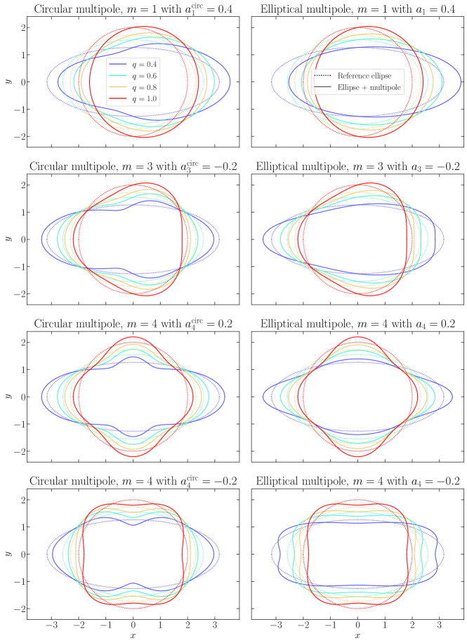
Figure 1: Patterns of perturbation corresponding to the $m=1$, $m=3$ and $m=4$ multipoles, in the circular (left) and elliptical (right) formulation, applied to reference ellipses with the same elliptical radius $R=2$ but varying axis ratio $q$. The multipoles are here aligned with the ellipses, i.e., $\phi_{m}=0$ or $\varphi_{m}=0$. Since the pattern itself does not depend on amplitude, we use values for $a_{m}^{\rm circ}$ and $a_{m}$ larger than physical expectations (of a few percent) for better visualization. The circular multipoles yield perturbation patterns that depend on the axis ratio, and that do not behave as expected for high ellipticities.

III.2 Elliptical multipoles

In order to overcome the flaws of the circular multipoles, we need a better parametrization - one that provides realistic, easily interpretable perturbations around elliptical countours without many additional parameters. For these “elliptical multipoles”, we simply adopt the definition that was originally used in isophote shape studies, which has the same shape as Equation (5) but uses different coordinates:

$$R\mapsto R+\delta R_{m}\text{ with }\delta R_{m}(\varphi)=a_{m}\cos(m(\varphi-\varphi_{m}))\ ,$$ (6)

where $R=\sqrt{qx^{2}+y^{2}/q}$ and $\varphi\equiv\arctan(qx,y)\pmod{2\pi}$ are the the elliptical radius and the eccentric anomaly, respectively (note the dependence on the axis ratio).

These perturbations are to a general ellipse what the circular multipoles are to a circle: if the axis ratio is $q=1$, we recover the same definition, but this time, the pattern of perturbation is being squished along with the ellipse for $q\neq 1$. The elliptical multipoles are therefore the “correct” formulation - in the sense that, regardless of the system’s ellipticity, they actually have the expected behavior of the multipole expansion. This means that the usual interpretations of the circular multipoles [e.g., 42] - true only if the reference contour is a circle, as we have discussed - can be extended to ellipses with any axis ratio [43]:

• the monopole ($m=0$ order) corresponds to a global rescaling - not useful in practice, since it is equivalent to a change in the Einstein radius.

• the dipole ($m=1$ order) encodes a skewness/lopsidedness in the convergence profile [e.g., 48, 67] - see Figure 2 for an illustration.

• the quadrupole ($m=2$ order) represents a global squeezing - not useful in practice, since the elliptical lens and external shear already have this complexity.

• the hexapole ($m=3$ order) and octupole ($m=4$ order) describe triangle-like and quadrangle-like deformations of the isocontours, respectively - see Figures 4 and 4. These are the most commonly considered perturbations in lensing [e.g., 40, 25, 30, 67]. From studies of galaxy isophotes, the $m=4$ is expected to have larger amplitudes than the $m=3$ (with typical fractional radial deviations along the major axis $a_{m}$ of the order of a percent), and to roughly align with the axis of the ellipse [35, 36, 41, 68] - in that case, the perturbation produces disky ($a_{m}>0$) or boxy ($a_{m}<0$) isophotes.

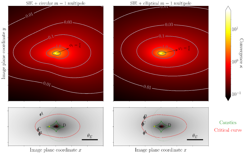
Figure 2: Top panel: Impact of a $m=1$ multipole on the convergence profile of a SIE lens model with axis ratio $q=0.5$, in the circular (left) and elliptical (right) formulations. We choose perturbations with direction $\phi_{1}=\frac{\pi}{6}$ (resp. $\varphi_{1}=\frac{\pi}{6}$), and with amplitude $a_{1}^{\rm circ}=0.175$ (resp. $a_{1}=0.175$) - larger than physical expectations, for better visualization. Bottom panel: Corresponding caustics, with an example of source position (yellow star) where the difference in formulation drastically changes the image positions and magnifications.

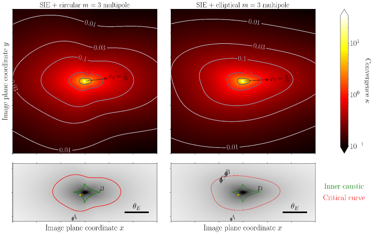
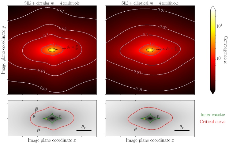
Figure 3: Same as Figure 2, but for a $m=3$ multipole with direction $\phi_{3}=\frac{\pi}{18}$ (resp. $\varphi_{3}=\frac{\pi}{18}$), and amplitude $a_{3}^{\rm circ}=0.06$ (resp. $a_{3}=0.06$).

Figure 4: Same as Figure 2, but for a $m=4$ multipole with direction $\phi_{4}=\frac{\pi}{24}$ (resp. $\varphi_{4}=\frac{\pi}{24}$), and amplitude $a_{4}^{\rm circ}=0.05$ (resp. $a_{4}=0.05$).

We can translate between the different coordinate systems using:

$$\begin{split}x&=r\cos{\phi}=R\cos{\varphi}/\sqrt{q}\\ y&=r\sin{\phi}=R\sin{\varphi}\sqrt{q}\end{split}$$ (7)

and the following equations are thus verified:

$$\begin{split}\frac{r}{R}(\phi;q)&=\frac{r}{\sqrt{qx^{2}+y^{2}/q}}=\frac{\sqrt{q}}{\sqrt{q^{2}\cos^{2}\phi+\sin^{2}\phi}}\\ \cos{\varphi(\phi;q)}&=\frac{q\cos\phi}{\sqrt{q^{2}\cos^{2}\phi+\sin^{2}\phi}}\\ \sin{\varphi(\phi;q)}&=\frac{\sin\phi}{\sqrt{q^{2}\cos^{2}\phi+\sin^{2}\phi}}\end{split}$$ (8)

For a given axis ratio $q$, we can define a bijective mapping between $\varphi\in\mathbb{R}$ and $\phi\in\mathbb{R}$:

$$\begin{split}\varphi(\phi;q)&=\arctan(q\cos\phi,\sin\phi)+\left[\phi-\arctan(\cos\phi,\sin\phi)\right]\\ \phi(\varphi;q)&=\arctan(\cos\varphi,q\sin\varphi)+\left[\varphi-\arctan(\cos\varphi,\sin\varphi)\right]\end{split}$$ (9)

For $q>0$, $\varphi(\phi;q)$ is an infinitely differentiable function of $\phi$ with first derivative

$$\frac{\partial\varphi}{\partial\phi}=\frac{q}{q^{2}\cos^{2}\phi+\sin^{2}\phi}$$ (10)

Since the mapping is bijective, a perturbation $(R,\varphi)\mapsto(R^{\prime},\varphi^{\prime})=(R+\delta R,\varphi)$ that is purely radial in the elliptical coordinates will also be purely radial in the usual polar coordinates ($\phi=\phi^{\prime}$ since $\varphi=\varphi^{\prime}$). Thus we can write $\delta r\cos\phi=\delta x=\delta R\cos\varphi/\sqrt{q}$, so that $\delta R/R=\delta x/x=\delta r/r$. The angular shape function corresponding to an elliptical multipole perturbation is therefore:

$$\begin{split}G_{m}(\phi;q,\varphi_{m})&=\delta r_{m}(\phi;q)=\delta R_{m}(\phi;q)\frac{r}{R}(\phi;q)\\ &=a_{m}\cos\left[m(\varphi(\phi;q)-\varphi_{m})\right]\frac{r}{R}(\phi;q)\\ &=a_{m}\sqrt{q}\cos(m\varphi_{m})G_{m}^{(1)}(\phi;q)+a_{m}\sqrt{q}\sin(m\varphi_{m})G_{m}^{(2)}(\phi;q)\end{split}$$ (11)

where we have defined

$$\begin{split}G_{m}^{(1)}(\phi;q)&\equiv\frac{1}{\sqrt{q}}\cos\left(m\cdot\varphi(\phi;q)\right)\frac{r}{R}(\phi;q)\\ &=T_{m}\left(\frac{q\cos\phi}{\sqrt{q^{2}\cos^{2}\phi+\sin^{2}\phi}}\right)\frac{1}{\sqrt{q^{2}\cos^{2}\phi+\sin^{2}\phi}}\\ \text{and }G_{m}^{(2)}(\phi;q)&\equiv\frac{1}{\sqrt{q}}\sin\left(m\cdot\varphi(\phi;q)\right)\frac{r}{R}(\phi;q)\\ &=U_{m-1}\left(\frac{q\cos\phi}{\sqrt{q^{2}\cos^{2}\phi+\sin^{2}\phi}}\right)\frac{\sin\phi}{q^{2}\cos^{2}\phi+\sin^{2}\phi}\end{split}$$ (12)

and $T_{m}$ (resp. $U_{m}$) are the Chebyshev polynomials of the first (resp. second) kind.

Since Poisson’s equation is linear, we can separately find the potentials $\psi_{m}^{(1)}(r,\phi;q)$ and $\psi_{m}^{(2)}(r,\phi;q)$ associated with $\kappa_{m}^{(1)}$ and $\kappa_{m}^{(2)}$ - the convergence profiles determined by shape functions $G_{m}^{(1)}(\phi;q)$ and $G_{m}^{(2)}(\phi;q)$ via Equation (1), respectively. We can then combine these two solutions with the adequate coefficients:

$$\psi_{m}(r,\phi;q)=a_{m}\sqrt{q}\cos(m\varphi_{m})\psi_{m}^{(1)}(r,\phi;q)+a_{m}\sqrt{q}\sin(m\varphi_{m})\psi_{m}^{(2)}(r,\phi;q)$$ (13)

Subsequently, if the potential is expressed as in Equation (1), the shape function can be separated in two components $F_{m}^{(1)}(\phi;q)$ and $F_{m}^{(2)}(\phi;q)$, respectively solving the differential Equation (2) for $G_{m}^{(1)}(\phi;q)$ and $G_{m}^{(2)}(\phi;q)$. Then, it can be expressed as

$$F_{m}(\phi;q)=a_{m}\sqrt{q}\cos(m\varphi_{m})F_{m}^{(1)}(\phi;q)+a_{m}\sqrt{q}\sin(m\varphi_{m})F_{m}^{(2)}(\phi;q).$$ (14)

We note, however, that the potential will not exactly follow the form of Equation (1) in the case of the circular multipole of order $m=1$ (see Section IV.1), and of the elliptical multipoles of order $m$ odd (see Sections IV.2, IV.3, and Appendix B.1).

The components of the convergence shape functions have the following symmetries:

$$\begin{split}G_{m}^{(i)}(\phi;q)&=G_{m}^{(i)}(\phi+2\pi;q)\text{ for }i=1,2\\ G_{m}^{(1)}(-\phi;q)&=G_{m}^{(1)}(\phi;q)\\ G_{m}^{(2)}(-\phi;q)&=-G_{m}^{(2)}(\phi;q)\\ G_{m}^{(1)}(\pi-\phi;q)&=(-1)^{m}G_{m}^{(1)}(\phi;q)\\ G_{m}^{(2)}(\pi-\phi;q)&=(-1)^{m-1}G_{m}^{(2)}(\phi;q)\\ \end{split}$$ (15)

so the components of the potential must, in theory, have the same symmetries. In the following, we will present some solutions to differential Equation (2) where all symmetries are not necessarily enforced, in which case we write them with a tilde: $\tilde{F}_{m}^{(i)}(\phi;q)$. We warn that these unsymmetrized shape functions cannot be directly plugged in Equation (1), and that direct symmetrization attempts might create some unwanted discontinuities (see Sections IV.1, IV.2, IV.3 and Appendix A.1).

We also remark that the expression in Equation (9) has the following property: $\varphi\left(\phi+\frac{\pi}{2};1/q\right)=\varphi\left(\phi;q\right)+\frac{\pi}{2}$, provided that we extend this definition of $\varphi$ to values $q>1$. Similarly, we can easily show that $\frac{r}{R}(\phi+\frac{\pi}{2};1/q)=\frac{r}{R}(\phi;q)$. Combining these two properties, we have the following invariance for the shape function $G_{m}$:

$$G_{m}\left(\phi+\frac{\pi}{2};\frac{1}{q},\varphi_{m}\right)=G_{m}\left(\phi;q,\varphi_{m}-\frac{\pi}{2}\right)$$ (16)

This can be interpreted in the following way: rotating the multipole by $90^{\circ}$ with respect to the ellipse is equivalent to rotating the entire system (i.e., both the ellipse and the multipole pertubation) by $90^{\circ}$, then exchanging the semi-major and semi-minor axis of the ellipse. We expect the potential $\psi_{m}(\phi;q)$ to have the same invariance - in particular, choosing $\varphi_{m}=0$ in Equation (16) for an odd integer $m=2k+1$, then making use of the decompositions in Equations (11) and (13), we obtain the following relation:

$$\psi_{2k+1}^{(2)}(r,\phi;q)=\frac{(-1)^{k+1}}{q}\psi_{2k+1}^{(1)}\left(r,\phi+\frac{\pi}{2};\frac{1}{q}\right)$$ (17)

Expressing this equation in cartesian coordinates $(x,y)$, taking derivatives, then transforming back to polar coordinates, we find similar relations for the deflection angles $\alpha_{x_{i},m}^{(j)}=\frac{\partial\psi_{m}^{(j)}}{\partial x_{i}}$ ($j=1,2$ and $x_{i}=x,y$), and for the components of the Hessian:

$$\left\{\begin{array}[]{l}\alpha_{x,2k+1}^{(2)}(r,\phi;q)=\frac{(-1)^{k+1}}{q}\alpha_{y,2k+1}^{(1)}(r,\phi+\frac{\pi}{2};\frac{1}{q})\\ \\ \alpha_{y,2k+1}^{(2)}(r,\phi;q)=\frac{(-1)^{k}}{q}\alpha_{x,2k+1}^{(1)}(r,\phi+\frac{\pi}{2};\frac{1}{q})\\ \\ \frac{\partial^{2}\psi_{2k+1}^{(2)}}{\partial x^{2}}(r,\phi;q)=\frac{(-1)^{k+1}}{q}\frac{\partial^{2}\psi_{2k+1}^{(1)}}{\partial y^{2}}(r,\phi+\frac{\pi}{2};\frac{1}{q})\\ \\ \frac{\partial^{2}\psi_{2k+1}^{(2)}}{\partial y^{2}}(r,\phi;q)=\frac{(-1)^{k+1}}{q}\frac{\partial^{2}\psi_{2k+1}^{(1)}}{\partial x^{2}}(r,\phi+\frac{\pi}{2};\frac{1}{q})\\ \\ \frac{\partial^{2}\psi_{2k+1}^{(2)}}{\partial x\partial y}(r,\phi;q)=\frac{(-1)^{k}}{q}\frac{\partial^{2}\psi_{2k+1}^{(1)}}{\partial x\partial y}(r,\phi+\frac{\pi}{2};\frac{1}{q})\end{array}\right.$$ (18)

For odd order $m$, since $\psi_{m}^{(2)}$ can be deduced from $\psi_{m}^{(1)}$, it means that determining $\psi_{m}^{(1)}(r,\phi;q)$ (i.e., the potential in the $\varphi_{m}=0$ case) is sufficient to get the full solution.

IV Lensing potential for the multipole perturbations

In this section, we describe the lensing potentials associated with the different multipole perturbations discussed in Section III. We start with the circular multipoles, paying particular attention to the special case of the circular $m=1$ order (section IV.1). Then, we present detailed solutions for the elliptical multipoles, in the three cases that will be most practical for lensing studies [e.g., 40, 25, 30, 10, 31, 32, 48, 67, 42]: the $m=1$ order (section IV.2), the $m=3$ order (section IV.3), and the $m=4$ order (section IV.4). The lensing potentials (and corresponding deflections angles) that are newly introduced in this section were implemented in the lens modeling package lenstronomy [49, 50] - used to generate Figures 2 to 9. Elliptical multipole lensing potentials for general $m\geq 2$ can be explicitly determined at the cost of lengthy calculations: for the sake of completeness, we present them in Appendix B.1 (for $m$ odd) and Appendix B.2 (for $m$ even).

IV.1 Lensing potential for the circular multipoles

The shape function for the lensing potential of the circular multipoles can be straightforwardly determined as [53, 61]:

$$F_{m}^{\rm circ}(\phi)=\frac{a_{m}^{\rm circ}}{1-m^{2}}\cos(m(\phi-\phi_{m}))\text{ for }m\neq 1$$ (19)

Equation (19) is no longer valid for $m=1$, so we need to treat this case separately. If we attempt to solve over all $\phi\in\mathbb{R}$ the differential Equation (2) for $G_{1}^{\rm circ}(\phi)=a_{1}^{\rm circ}\cos(\phi-\phi_{1})$, we find the following solution :

$$\tilde{F}_{1}^{\rm circ}(\phi)=\frac{a_{1}^{\rm circ}}{2}(\phi-\phi_{1})\sin(\phi-\phi_{1})+A_{1}^{\rm circ}\cos(\phi-\phi_{1})+B_{1}^{\rm circ}\sin(\phi-\phi_{1})$$ (20)

where $A_{1}^{\rm circ}$ and $B_{1}^{\rm circ}$ are constants, that have no impact on the lensing observables due to the prismatic degeneracy (see Section II or [59]).

The problem is that this solution does not have the expected symmetries: like $G_{1}^{\rm circ}(\phi)$, the shape function for the potential should be $2\pi$-periodic, $\phi-\phi_{1}\mapsto\pi-(\phi-\phi_{1})$ antisymmetric and $\phi-\phi_{1}\mapsto-(\phi-\phi_{1})$ symmetric. If we choose $B_{1}^{\rm circ}=0$, the last symmetry is enforced in Equation (20), but not the first two, no matter how we choose $A_{1}^{\rm circ}$. One can attempt to symmetrize the shape function, but this can only be achieved at the expense of its differentiability: in Appendix A.1, we show how symmetrizing a potential of the form (1) creates jump discontinuities in the deflection field. We want a potential that is solution of the Poisson equation over the entire domain $\mathbb{R}^{2}\setminus\{\mathbf{0}\}$ ($\mathbf{0}$ being a singular point for the SIE anyways), and not defined piecewise - in fact, for a given source/lens configuration, the lensing potential must be differentiable over a contiguous region connecting the positions of all images in order to be physically meaningful [57]. This means that there cannot be jump discontinuities in the deflection field.

This difficulty can be overcome by dropping the assumption that the potential has to be written as in Equation (1), e.g., by allowing radial dependencies other than $\psi\propto r$. We propose the following lensing potential:

$$\psi_{1}^{\rm circ}(r,\phi)=\frac{a_{1}^{\rm circ}}{2}r\ln\left(\frac{r}{r_{E}}\right)\cos(\phi-\phi_{1})$$ (21)

which is twice differentiable over $\mathbb{R}^{2}\setminus\{\mathbf{0}\}$, solves Poisson’s equation for the convergence of the $m=1$ circular multipole $\kappa_{1}^{\rm circ}(r,\phi)=a_{1}^{\rm circ}\frac{\cos(\phi-\phi_{1})}{2r}$ , and has all the correct symmetries. Its derivatives are given by:

$$\left\{\begin{array}[]{l}\alpha_{x,1}^{\rm circ}(r,\phi)=\frac{\partial\psi_{1}^{\rm circ}}{\partial x}=\frac{a_{1}^{\rm circ}}{2}\left[\cos\phi_{1}\ln\left(\frac{r}{r_{E}}\right)+\cos(\phi-\phi_{1})\cos\phi\right]\\ \\ \alpha_{y,1}^{\rm circ}(r,\phi)=\frac{\partial\psi_{1}^{\rm circ}}{\partial y}=\frac{a_{1}^{\rm circ}}{2}\left[\sin\phi_{1}\ln\left(\frac{r}{r_{E}}\right)+\cos(\phi-\phi_{1})\sin\phi\right]\\ \\ \frac{\partial^{2}\psi_{1}^{\rm circ}}{\partial x^{2}}(r,\phi)=\frac{a_{1}^{\rm circ}}{2r}\left[2\cos\phi_{1}\cos\phi-\cos(\phi-\phi_{1})\cos(2\phi)\right]\\ \\ \frac{\partial^{2}\psi_{1}^{\rm circ}}{\partial y^{2}}(r,\phi)=\frac{a_{1}^{\rm circ}}{2r}\left[2\sin\phi_{1}\sin\phi+\cos(\phi-\phi_{1})\cos(2\phi)\right]\\ \\ \frac{\partial^{2}\psi_{1}^{\rm circ}}{\partial x\partial y}(r,\phi)=\frac{a_{1}^{\rm circ}}{2r}\left[\sin(\phi+\phi_{1})-\cos(\phi-\phi_{1})\sin(2\phi)\right]\\ \\ \end{array}\right.$$ (22)

Additional arguments in favor of this potential are presented in Appendix A.2: namely, equivalent solutions are found when taking the limit $\gamma\mapsto 2$ after generalizing circular multipole perturbations to non-isothermal profiles (Appendix A.2.1), and when using direct integration to calculate the deflection angles in the complex formulation of gravitational lensing (Appendix A.2.2). We present example maps of this lensing potential and deflection angles for the circular $m=1$ multipole in Figure 5.

The normalizing radius $r_{E}$, introduced in Equations (21) and (22), modulates a term $\propto r\cos(\phi-\phi_{1})$ in the lensing potential. Therefore, as a consequence of the prismatic degeneracy (see Section II or [59]), it does not have any impact on the lensing observables. We choose the following convention: $r_{E}=\theta_{E}$, such that $\vec{\alpha}_{1}^{\rm\ circ}(\theta_{E},\phi_{1}\pm\pi/2)=0$, i.e., at the Einstein radius, in the direction orthogonal to the multipole orientation, the additional deflection from the multipole is zero (see Figure 5).

IV.2 The $m=1$ elliptical multipole lensing potential

For the elliptical $m=1$ multipole, we use the decomposition of the convergence and potential introduced in Equations (11) and (13). We start with the case where $\varphi_{1}=0$, by solving the differential equation:

$$F_{1}^{(1)\prime\prime}(\phi;q)+F_{1}^{(1)}(\phi;q)=G_{1}^{(1)}(\phi;q)=\frac{\cos\phi}{q^{2}\cos^{2}\phi+\sin^{2}\phi}$$ (23)

where ^′ still denotes the derivative with respect to $\phi$. We find the following solution over $\phi\in\mathbb{R}$:

$$\tilde{F_{1}}^{(1)}(\phi;q)=\frac{1}{1-q^{2}}\Big{[}-\frac{q}{2}\cos(\phi)\ln\left(1+q^{2}+(q^{2}-1)\cos(2\phi)\right)+A_{1}^{(1)}\cos\phi+B_{1}^{(1)}\sin\phi\\ -\sin(\phi)\left[q\phi-\varphi(\phi;q)\right]\Big{]}$$ (24)

where $A_{1}^{(1)}(q),B_{3}^{(1)}(q)$ are “constants” (i.e., independent of $\phi$, they can still depend on the axis ratio $q$), and we use Equation (9) for the definition of $\varphi(\phi;q)$.

Unfortunately, this has the same issues as $\tilde{F}_{1}^{\rm circ}(\phi)$ for the circular $m=1$ case: the expected symmetries ($2\pi$ periodicity, $\phi\mapsto-\phi$ symmetry, $\phi\mapsto\pi-\phi$ antisymmetry) are not enforced, because of the term in $(q\phi-\varphi(\phi,q))\sin\phi$ this time. Once again, trying to symmetrize the shape function directly leads to discontinuities in the deflection angle. To remedy this issue, we recognize that the expression $\phi-\varphi(\phi,q)$ (note the equal coefficients) is $2\pi$ periodic, and antisymmetric under $\phi\mapsto-\phi$ and $\phi\mapsto\pi-\phi$. In turn, the following “modified” shape function

$$\begin{split}\hat{F}_{1}^{(1)}(\phi;q)&\equiv\tilde{F}_{1}^{(1)}(\phi;q)-\frac{1-q}{1-q^{2}}\phi\sin\phi\\ &=\tilde{F}_{1}^{(1)}(\phi;q)-\lambda_{1}(q)\cdot\tilde{F}_{1}^{\rm circ}(\phi)\Big{|}_{\phi_{1}=0,a_{1}^{\rm circ}=1}\text{ with }\lambda_{1}(q)\equiv\frac{2}{1+q}\end{split}$$ (25)

has the correct symmetries expected from the $m=1$ shape function, provided that we choose $B_{1}^{(1)}=0$ for the $\phi\mapsto-\phi$ symmetry. This function has the added benefit of being infinitely differentiable with respect to $\phi$: in particular, it corresponds to a potential that has continuous deflection angles in $\mathbb{R}^{2}\setminus\{\mathbf{0}\}$. The convergence profile associated with this shape function is $\frac{1}{2r}[\hat{F}_{1}^{(1)\prime\prime}(\phi;q)+\hat{F}_{1}^{(1)}(\phi;q)]=\frac{G_{1}^{(1)}(\phi;q)}{2r}-\lambda_{1}(q)\frac{\cos\phi}{2r}$, which is the profile we desire minus a $m=1$ circular multipole component. Therefore, by decomposing the potential as

$$\psi_{1}^{(1)}(r,\phi;q)=r\hat{F}_{1}^{(1)}(\phi;q)+\lambda_{1}(q)\cdot\psi_{1}^{\rm circ}\left(r,\phi\right)\Big{|}_{\phi_{1}=0,a_{1}^{\rm circ}=1}$$ (26)

we have found a solution for the first component of the $m=1$ elliptical multipole that has (a) the correct symmetries, and (b) no discontinuities in the deflection field. Derivatives of this potential are obtained by combining (with the appropriate coefficients) Equation (3) with the shape function $\hat{F}_{1}^{(1)}(\phi;q)$ and Equation (22).

The constants $A_{1}^{(1)}$ and $B_{1}^{(1)}$ are a priori not constrained because of the prismatic degeneracy, but we actually need to take $B_{1}^{(1)}=0$ if we want to enforce the $\phi\mapsto-\phi$ symmetry. $A_{1}^{(1)}$ cannot be determined by symmetries alone, but we can choose its value to ensure the convergence to the circular solution in the limit $q\to 1$. Since $\lambda_{1}(q)\mathrel{\underset{q\to 1}{\longrightarrow}}1$, we want $\hat{F}_{1}^{(1)}(\phi;q)\mathrel{\underset{q\to 1}{\longrightarrow}}0$, or equivalently $\tilde{F}_{1}^{(1)}(\phi;q)\mathrel{\underset{q\to 1}{\longrightarrow}}\tilde{F}_{1}^{\rm circ}(\phi)\Big{|}_{\phi_{1}=0,a_{1}^{\rm circ}=1}=\frac{1}{2}\phi\sin\phi$. Performing a Taylor expansion of Equation (24) in $(1-q)$, we find:

$$\tilde{F_{1}}^{(1)}(\phi;q)\mathrel{\underset{q\to 1}{=}}\frac{A_{1}^{(1)}}{1-q^{2}}\cos\phi-\frac{\ln(2)}{4(1-q)}\cos\phi+\frac{4+\ln(2)}{8}\cos\phi+\frac{1}{2}\phi\sin\phi+O[1-q]\\$$ (27)

so, in order to converge to the circular multipole solution, we need

$$A_{1}^{(1)}(q)=\frac{\ln 2}{4}(1+q)-\frac{1-q^{2}}{2}\left(1+\frac{\ln 2}{4}\right)+f(q)\text{ with }(1-q)f(q)\mathrel{\underset{q\to 1}{\longrightarrow}}0$$ (28)

Because of the prismatic degeneracy we can choose any function $f(q)$ without changing the lensing observables, and as long as $(1-q)f(q)\mathrel{\underset{q\to 1}{\longrightarrow}}0$ the potential will converge to the adequate limit when $q\to 1$. We therefore choose the simplest solution by taking $f(q)=0$ in Equation (28).

The discussion above fully describes the elliptical $m=1$ potential in the case where $\varphi_{1}=0$. In order to obtain the more general solution for any $\varphi_{1}$, we need to determine the other component $\psi_{1}^{(2)}$ of the decomposition presented in Equation (13). For this, we can simply exploit the invariance established earlier in Equations (17) and (18): in particular, we have $\psi_{1}^{(2)}(r,\phi;q)=-\frac{1}{q}\psi_{1}^{(1)}\left(r,\phi+\frac{\pi}{2};\frac{1}{q}\right)$. We note that this automatically ensures the convergence of $\psi_{1}^{(2)}$ to the $\phi_{1}=\pi/2$ circular solution when $q\mapsto 1$. We present example maps of the lensing potential and deflection angles for the $m=1$ elliptical multipole in Figure 5, where they are compared to the $m=1$ circular multipole solution.

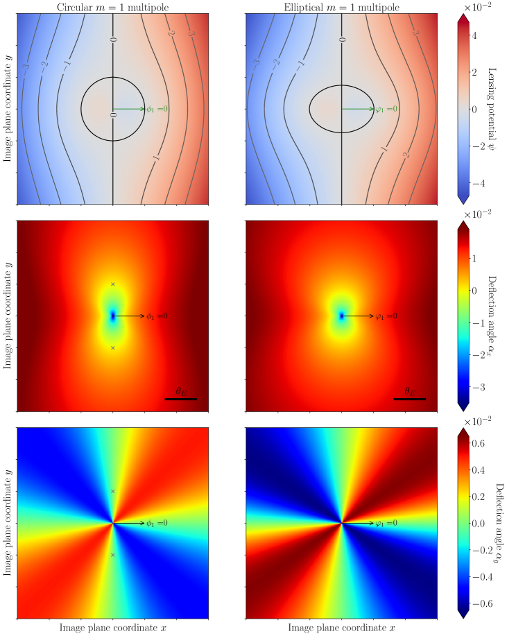
Figure 5: Example of lensing potential $\psi$ (top panel) and deflection angles $\alpha_{x}$ (middle panel) and $\alpha_{y}$ (bottom panel) associated with a $m=1$ multipole perturbation in the circular (left) and elliptical (right) formulations. We use direction $\phi_{1}=0$ (resp. $\varphi_{1}=0$), amplitude $a_{1}^{\rm circ}=0.02$ (resp. $a_{1}=0.02$), and axis ratio $q=0.5$ for the elliptical multipole. The grey crosses are located at the Einstein radius in the direction orthogonal to $\phi_{1}$, where $\alpha_{x}=\alpha_{y}=0$ thanks to our choice of $r_{E}$.

IV.3 The $m=3$ elliptical multipole lensing potential

We start by finding a solution for the $m=3$ only, $\varphi_{3}=0$ case, i.e., for the differential equation:

$$F_{3}^{(1)\prime\prime}(\phi;q)+F_{3}^{(1)}(\phi;q)=G_{3}^{(1)}(\phi;q)=\frac{4q^{3}\cos^{3}\phi}{\left(q^{2}\cos^{2}\phi+\sin^{2}\phi\right)^{2}}-\frac{3q\cos\phi}{q^{2}\cos^{2}\phi+\sin^{2}\phi}$$ (29)

where we have used $T_{3}(x)=4x^{3}-3x$ in Equation (12). The solution over all $\phi\in\mathbb{R}$ is:

$$\begin{split}\tilde{F_{3}}^{(1)}(\phi;q)=\frac{1}{2(1-q^{2})^{2}}\Big{[}&\cos(\phi)q\left(3+q^{2}\right)\ln\left(1+q^{2}+(q^{2}-1)\cos(2\phi)\right)+2A_{3}^{(1)}\cos\phi\\ &+2B_{3}^{(1)}\sin\phi+2\sin(\phi)\left[q\left(3+q^{2}\right)\phi-\left(1+3q^{2}\right)\varphi(\phi;q)\right]\Big{]}\end{split}$$ (30)

where $A_{3}^{(1)}(q),B_{3}^{(1)}(q)$ are constants in the same sense as before, i.e., independent of $\phi$. We note that the expected $\phi\mapsto-\phi$ symmetry can be enforced in Equation (30) if, and only if, $B_{3}^{(1)}=0$; but that this expression cannot be $2\pi$-periodic or $\phi\mapsto\pi-\phi$ antisymmetric because of the terms in $\phi$ and $\varphi(\phi;q)$. This causes the same problem as in Sections IV.1 and IV.2: the shape function cannot be properly symmetrized without creating discontinuities in the deflection field. Instead, we use the same trick as in Section IV.2, breaking the potential into a component ($\propto r$) with a shape function having the correct symmetries, and a circular $m=1$ multipole component ($\propto r\ln r$):

$$\psi_{3}^{(1)}(r,\phi;q)=r\hat{F}_{3}^{(1)}(\phi;q)+\lambda_{3}(q)\cdot\psi_{1}^{\rm circ}\left(r,\phi\right)\Big{|}_{\phi_{1}=0,a_{1}^{\rm circ}=1}$$ (31)

where we have defined $\lambda_{3}(q)=-\frac{2(1-q)}{(1+q)^{2}}$ and

$$\begin{split}\hat{F}_{3}^{(1)}(\phi;q)&=\tilde{F_{3}}^{(1)}(\phi;q)-\frac{\lambda_{3}(q)}{2}\phi\sin\phi\\ &=\tilde{F_{3}}^{(1)}(\phi;q)-\lambda_{3}(q)\cdot\tilde{F}_{1}^{\rm circ}(\phi)\Big{|}_{\phi_{1}=0,a_{1}^{\rm circ}=1}\\ \end{split}$$ (32)

The additional term in $\lambda_{3}(q)$ equalizes the coefficients in front of $\phi$ and $\varphi(\phi;q)$ in Equation (30): thanks to the properties of $\phi-\varphi(\phi,q)$ (see Section IV.2), this means that $\hat{F}_{3}^{(1)}(\phi;q)$ is $2\pi$ periodic, symmetric under $\phi\mapsto-\phi$ and antisymmetric under $\phi\mapsto\pi-\phi$, provided that we choose $B_{3}^{(1)}=0$.

The value of $A_{3}^{(1)}(q)$ cannot be chosen from symmetries alone. Adopting the same approach as for the $m=1$ case, we look to match our solution with the circular multipole solution when $q\to 1$. In this limit, $\lambda_{3}(q)\to 0$, so we want $\tilde{F_{3}}^{(1)}(\phi;q)\mathrel{\underset{q\to 1}{\longrightarrow}}F_{3}^{\rm circ}(\phi)\Big{|}_{\phi_{3}=0,a_{3}^{\rm circ}=1}=-\frac{1}{8}\cos(3\phi)$. Performing the Taylor expansion of Equation (30):

$$\begin{split}\tilde{F_{3}}^{(1)}(\phi;q)\mathrel{\underset{q\to 1}{=}}\frac{A_{3}^{(1)}}{(1-q^{2})^{2}}\cos\phi+\frac{\ln(2)\cos\phi}{2(1-q)^{2}}-\frac{(4+\ln(2))\cos\phi}{4(1-q)}+\frac{1}{2}\cos\phi\sin^{2}\phi+O[1-q]&\\ \mathrel{\underset{q\to 1}{=}}\frac{A_{3}^{(1)}}{(1-q^{2})^{2}}\cos\phi+\frac{\ln(2)\cos\phi}{2(1-q)^{2}}-\frac{(4+\ln(2))\cos\phi}{4(1-q)}+\frac{1}{8}\cos\phi-\frac{1}{8}\cos(3\phi)+O[1-q]&\end{split}$$ (33)

so, in order to converge to the $\phi_{3}=0$ circular multipole solution, we take:

$$A_{3}^{(1)}(q)=-\frac{(1+q)^{2}}{2}\left[\ln(2)-2(1-q)\left(1+\frac{\ln(2)}{4}\right)+\frac{(1-q)^{2}}{4}\right].$$ (34)

Once again, because of the prismatic degeneracy, we could add any term $f(q)$ to $A_{3}^{(1)}$ as long as $f(q)(1-q)^{-2}\mathrel{\underset{q\to 1}{\longrightarrow}}0$ without changing the lensing observables, so we choose $f(q)=0$ for simplicity.

To find the general solution for the $m=3$ case, we still need to find $\psi_{3}^{(2)}$, i.e., solve the potential in the case where $3\varphi_{3}=\pi/2$. Like in Section IV.2, we can simply exploit the invariance described by Equation (17), writing:

$$\psi_{3}^{(2)}(r,\phi;q)=\frac{1}{q}\psi_{3}^{(1)}\left(r,\phi+\frac{\pi}{2};\frac{1}{q}\right)$$ (35)

which automatically ensures that the limit $q\mapsto 1$ matches the circular solution. We showcase example maps of the lensing potential and deflection angles for the $m=3$ elliptical multipole in Figure 6, where they are compared to the $m=3$ circular multipole maps. We present an even more general solution, valid for any $m\geq 2$ odd, in Appendix B.1.

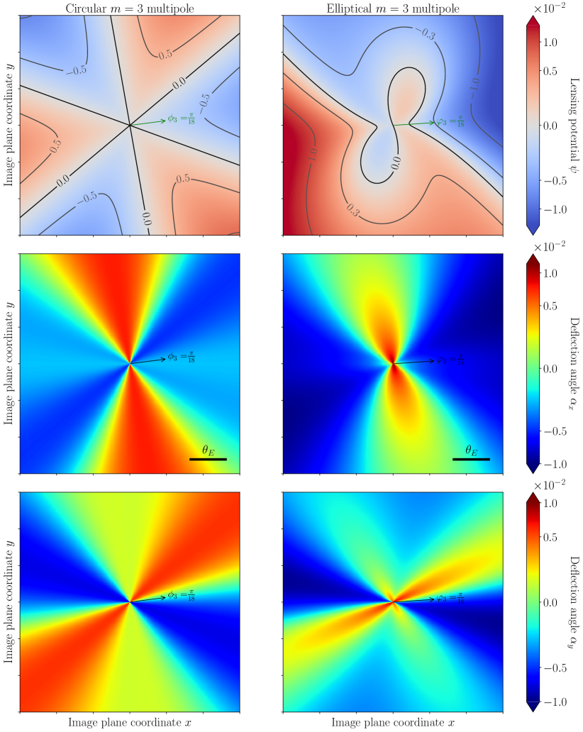
Figure 6: Same as Figure 5, but for a $m=3$ multipole with direction $\phi_{3}=\frac{\pi}{18}$ (resp. $\varphi_{3}=\frac{\pi}{18}$), and amplitude $a_{3}^{\rm circ}=0.02$ (resp. $a_{3}=0.02$). The elliptical multipole still has axis ratio $q=0.5$.

IV.4 The $m=4$ elliptical multipole lensing potential

For the $m=4$ case, we give explicit solutions for $F_{4}^{(1)}(\phi;q)$ and $F_{4}^{(2)}(\phi;q)$, which are respectively solutions of the following differential equations:

$$\begin{split}F_{4}^{(1)\prime\prime}(\phi;q)+F_{4}^{(1)}(\phi;q)&=G_{4}^{(1)}(\phi;q)=\frac{1}{\sqrt{q^{2}\cos^{2}\phi+\sin^{2}\phi}}-\frac{8q^{2}\sin^{2}\phi\cos^{2}\phi}{(q^{2}\cos^{2}\phi+\sin^{2}\phi)^{5/2}}\\ F_{4}^{(2)\prime\prime}(\phi;q)+F_{4}^{(2)}(\phi;q)&=G_{4}^{(2)}(\phi;q)=\frac{8q^{3}\sin\phi\cos^{3}\phi}{(q^{2}\cos^{2}\phi+\sin^{2}\phi)^{5/2}}-\frac{4q\sin\phi\cos\phi}{(q^{2}\cos^{2}\phi+\sin^{2}\phi)^{3/2}}\end{split}$$ (36)

where we have used $T_{4}(x)=8x^{4}-8x^{2}+1$ and $U_{3}(x)=8x^{3}-4x$ in Equation (12). The solutions over all $\phi\in\mathbb{R}$ are:

$$\begin{split}F_{4}^{(1)}(\phi;q)=&\frac{-4\sqrt{2}\left(1+4q^{2}+q^{4}+(q^{4}-1)\cos(2\phi)\right)}{3\left(1-q^{2}\right)^{2}\sqrt{1+q^{2}+(q^{2}-1)\cos(2\phi)}}\\ &+\frac{1+6q^{2}+q^{4}}{(1-q^{2})^{5/2}}\left[A_{4}^{(1)}\cos\phi+\cos(\phi)\arctan\left(\frac{\sqrt{2(1-q^{2})}\cos(\phi)}{\sqrt{1+q^{2}+(q^{2}-1)\cos(2\phi)}}\right)\right.\\ &\left.+B_{4}^{(1)}\sin\phi+\sin(\phi)\log\left(\frac{\sqrt{1-q^{2}}\sin(\phi)}{q}+\sqrt{1+\frac{(1-q^{2})}{q^{2}}\sin^{2}(\phi)}\right)\right]\end{split}$$ (37)

$$\begin{split}\text{and }F_{4}^{(2)}(\phi;q)=&\ \frac{-4\sqrt{2}\ q\sin(2\phi)}{3(1-q^{2})\sqrt{1+q^{2}+(q^{2}-1)\cos(2\phi)}}\\ &+\frac{4q(1+q^{2})}{(1-q^{2})^{5/2}}\left[A_{4}^{(2)}\cos\phi-\sin(\phi)\arctan\left(\frac{\sqrt{2(1-q^{2})}\cos(\phi)}{\sqrt{1+q^{2}+(q^{2}-1)\cos(2\phi)}}\right)\right.\\ &\left.+B_{4}^{(2)}\sin\phi+\cos(\phi)\log\left(\frac{\sqrt{1-q^{2}}\sin(\phi)}{q}+\sqrt{1+\frac{(1-q^{2})}{q^{2}}\sin^{2}(\phi)}\right)\right]\end{split}$$ (38)

We note that these expressions are already $2\pi$-periodic, and that they have the correct symmetries:

$$\begin{split}F_{4}^{(1)}(\phi;q)&=F_{4}^{(1)}(\pi-\phi;q)=F_{4}^{(1)}(-\phi;q)\\ F_{4}^{(2)}(\phi;q)&=-F_{4}^{(2)}(\pi-\phi;q)=-F_{4}^{(2)}(-\phi;q)\end{split}$$ (39)

if, and only if, we take $A_{4}^{(1)}=B_{4}^{(1)}=A_{4}^{(2)}=B_{4}^{(2)}=0$. Furthermore, the $q\to 1$ limit is already matching the circular multipole solution: we have, for all $\phi\in\mathbb{R}$,

$$\begin{split}F_{4}^{(1)}(\phi;q)&\mathrel{\underset{q\to 1}{\longrightarrow}}-\frac{1}{15}\cos(4\phi)=F_{4}^{\rm circ}(\phi)\Big{|}_{\phi_{4}=0,\ a_{4}^{\rm circ}=1}\\ \text{ and }F_{4}^{(2)}(\phi;q)&\mathrel{\underset{q\to 1}{\longrightarrow}}-\frac{1}{15}\sin(4\phi)=F_{4}^{\rm circ}(\phi)\Big{|}_{4\phi_{4}=\pi/2,\ a_{4}^{\rm circ}=1}.\end{split}$$ (40)

Subsequently, the potential is directly obtained by plugging $F_{4}^{(1)}(\phi;q)$ and $F_{4}^{(2)}(\phi;q)$ in Equation (14), then using the resulting shape function $F_{4}(\phi;q)$ in Equation (1) - in particular, there is no need to split the potential into a $\propto r$ and a $\propto r\ln r$ component like for the $m=1$ and $m=3$ cases. The $m=4$ elliptical lensing potential is thus determined: in Figure 7, we display example maps of this potential and of the associated deflection angles, and compare them to the $m=4$ circular multipole maps. We present an even more general solution, valid for any $m\geq 2$ even, in Appendix B.2.

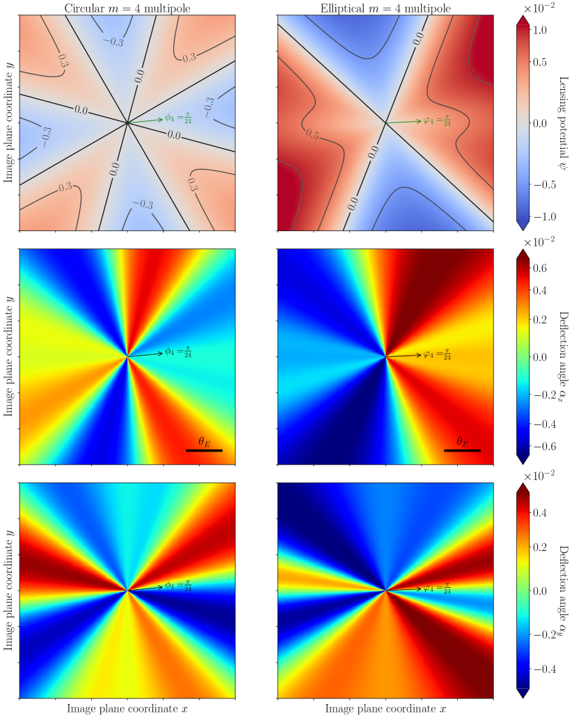
Figure 7: Same as Figure 5, but for a $m=4$ multipole with direction $\phi_{4}=\frac{\pi}{24}$ (resp. $\varphi_{4}=\frac{\pi}{24}$), and amplitude $a_{4}^{\rm circ}=0.02$ (resp. $a_{4}=0.02$). The elliptical multipole still has axis ratio $q=0.5$.

V Example application: Flux-ratio anomalies

Strong gravitational lensing offers a unique opportunity to directly probe the properties of DM on small scales, without relying on baryonic tracers. Strong lens systems in which a quasar becomes quadruply imaged are particularly worthy of attention: the flux ratios (i.e., the relative magnifications between lensed images) that are observed frequently disagree with the prediction made by smooth macromodels of the lensing galaxy. These “flux-ratio anomalies” are usually thought to be caused by the additional, localized gravitational fields associated with dark substructure (i.e., DM subhalos within the main lens) or DM halos along the line of sight. Since the abundance, mass function and internal density profiles of these halos depend on the nature of DM, population-level statistics of flux-ratio anomalies can be used to test the CDM paradigm and place constraints on various alternative DM models [69, 70, 71, 61, 72, 73, 74, 4, 3, 29, 75, 76, 5, 77, 10].

These methods require careful modeling, since they implicitely assume that the macromodel is accurate enough to statistically make reliable predictions of the flux ratio in the absence of substructure. In individual systems, specific configurations of azimuthal structure can mimick the effect of DM halos on flux ratios, so sufficient model flexibility is essential to ensure that the statistics of flux-ratio anomalies are unbiased [30, 31, 10, 32]. For this reason, recent studies have included (circular) multipole terms in their macromodels, primarily the $m=1$, $m=3$ and $m=4$ orders [e.g., 5, 32, 67, 41].

In our improved elliptical multipole formalism, the parameters and patterns of perturbation around the ellipse are distinct from the circular case, thus the amount of flux-ratio perturbations that can be attributed to such terms should also differ. We investigated the impact of the change in formulation by conducting the following experiment. We considered two reference mock lensed systems, generated using an EPL profile with isothermal slope and non-negligible ellipticities (one with $q=0.73$ and one with $q=0.58$), plus an external shear term, and a point source placed inside the inner caustic in order to produce four images. We then added $m=1$, $m=3$, and $m=4$ multipole terms with directions and amplitudes randomly sampled from physically motivated distributions. Finally, keeping these perturbations fixed, we adjusted the other degrees of freedom in the macromodel (source position and EPL + shear parameters) in order to recover the initial image positions, assuming an astrometric precision of $5$ mas [32]. We adopted uniform priors on $[-\pi,\pi]$ for the direction of the multipoles relative to the reference ellipse ($\phi_{m}$ or $\varphi_{m}$), and Gaussian priors informed by isophotal shape studies for the amplitudes ($a_{m}^{\rm circ}$ or $a_{m}$) - with mean $0$ and standard deviation $0.005$, $0.005$, and $0.01$ for the $m=1$, $m=3$, and $m=4$ orders, respectively [e.g., 48, 36]. After taking $15000$ samples of the multipole configurations, we compared the distribution of flux ratios obtained with the elliptical versus the circular formulation. These distributions, shown in Figures 9 and 9, and can be essentially interpreted as conditional probability distributions $\mathbf{p}(\text{flux ratios}\big{|}\text{image positions})$, assuming an EPL + shear + $m=1$ + $m=3$ + $m=4$ lens model (without substructure) with the chosen priors on multipole parameters.

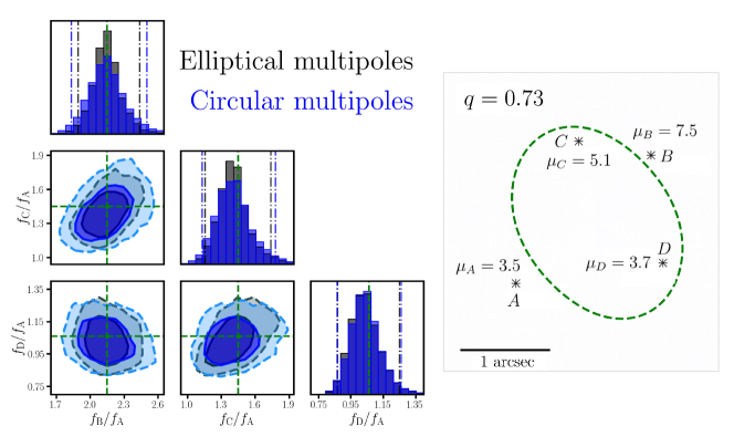
Figure 8: Distribution of flux ratios calculated from 15000 EPL + shear + $m=1$ + $m=3$ + $m=4$ lens models with axis ratio $q=0.73$, identical image positions, and randomly sampled multipole parameters, in the elliptical vs circular formulation. The 2D contours enclose 68% and 95% credible regions, and the vertical dosh-dotted bars in the marginal distributions represent 95% credible intervals. The right panel shows a schematic view of the image positions and magnifications, and of the lens critical curve in the EPL+shear case (i.e., without multipoles); the corresponding flux ratios are indicated by the green crosshairs.

Figure 9: Same as Figure 9, but for lens models with axis ratio $q=0.58$.

As Figures 9 and 9 illustrate, the inclusion of multipoles with either formulation can generate substantial perturbations to the flux ratios predicted by the fiducial model (i.e., the one with a purely elliptical lens + external shear). The circular multipoles, however, tend to produce larger flux-ratio perturbations compared to the elliptical version (in particular, the distributions have wider wings). We can quantify this by examining, over all multipole realizations, the median $\mu_{\rm pert}$ of the strongest relative flux-ratio perturbation:

$$\mu_{\rm pert}=\text{med}\left(\max_{i\neq j}\left|\frac{(f_{i}/f_{j})-(f_{i}/f_{j})_{\rm EPL+shear}}{(f_{i}/f_{j})_{\rm EPL+shear}}\right|\right),$$ (41)

which is consistently larger for the circular multipoles (i.e., $\mu_{\rm pert}^{\rm circ}>\mu_{\rm pert}^{\rm ell}$). This is unsurprising given the fact that, for multipoles of equal amplitude applied to systems that are not near-circular, the circular perturbations yield convergence profiles displaying structure that is more localized and physically less realistic (see Section III.1) than their elliptical counterpart (see Figures 2, 4, and 4). As expected from this interpretation, the difference becomes more apparent for highly flattened systems: in the examples shown here, distributions differ more for $q=0.58$ (Figure 9) than for $q=0.73$ (Figure 9). In particular, circular multipoles generate flux-ratio perturbations that are typically 20% larger ($\frac{\mu_{\rm pert}^{\rm circ}}{\mu_{\rm pert}^{\rm ell}}\approx 1.2$) for $q=0.73$, and typically 50% larger ($\frac{\mu_{\rm pert}^{\rm circ}}{\mu_{\rm pert}^{\rm ell}}\approx 1.5$) for $q=0.58$.

VI Summary & Discussion

In this work, we have illustrated the shortcomings of the circular multipoles, a formalism commonly used to represent deviations from ellipticity in models of lensing galaxies. We have argued that these perturbations produce patterns that depend on the axis ratio, and that do not correspond to physical expectations for systems that are not near-circular. We have proposed an improved formulation, the elliptical multipoles, applicable to elliptical profiles with any axis ratio. We have introduced solutions for the lensing potentials of these elliptical multipoles (as well as for the $m=1$ circular multipole), taking particular care to ensure that the expected symmetries and behavior in limiting cases were respected. We have compared the two formulations in the context of a physical application: flux-ratio anomalies of quadruply imaged quasars. Our results suggest that circular multipoles produce flux-ratio perturbations that are typically larger than the elliptical multipoles, especially for highly flattened system, likely due to the unrealistic perturbations introduced by circular multipoles outisde of the near-circular regime.

We note that, while the elliptical multipole expansion provides a better parametrization than the circular formulation, it still operates under the assumption that the reference lens mass model is an isothermal profile. In other terms, our solution will be exact only if the 3D density profile $\rho(r_{\rm 3D})\propto r_{\rm 3D}^{-\gamma}$ has a slope $\gamma=2$. Since astrophysical lenses are typically near-isothermal (e.g., the average value and dispersion in the SLACS survey are respectively $\langle\gamma\rangle=2.08\pm 0.03,\sigma_{\gamma}=0.16\pm 0.02$ [78, 79]), the formalism proposed here remains a good approximation. For this reason, the user-ready mass models implemented in lenstronomy combine the isothermal multipoles presented here with EPL profiles (i.e., with a free slope $\gamma$). There exists an exact generalization of the circular multipoles for non-isothermal slopes (see [26, 67] and Appendix A.2.1), available for instance in the strong lensing package PyAutoLens [80, 81, 82]. We caution, however, that current implementations diverge when $\gamma\to 2$ in the case of the $m=1$ multipole (we discuss this further in Appendix A.2.1 and propose a way to remedy this issue). Given the complexity of the potentials presented in Section IV and Appendix B for the isothermal case, we leave to future work the extension of the elliptical multipoles to non-isothermal slopes.

We also remark that, in real lens systems, departures from pure elliptical profiles can manifest themselves in more than one way. The addition of multipoles (and in particular the $m=1$, $m=3$, and $m=4$ orders) is a popular choice, and one that is physically motivated by studies of galaxy isophotal shapes, but it might not fully capture this additional complexity. For instance, massive elliptical galaxies can display ellipticity gradients or isophotal twisting (i.e., a change with radius of the principal axis of the isophotes, which would trace a similar twisting in the isodensity contours) [e.g., 33, 83, 36, 37, 84, 85]. Some of the more elongated lensing galaxies could also harbor an additional baryonic edge-on disk component perturbing the flux ratios, which is not exactly the same as having a disky mass distribution [86, 87]. Even in the context of multipole perturbations, the amplitude $a_{m}$ of the deviation from ellipticity is a priori different for each isocontour - isophotal shape studies usually measure full radial profiles for the multipole amplitude [e.g., 33, 35, 45, 43, 46, 48]. Therefore, the multipole terms used in lensing (parametrized with a constant amplitude relative to the semi-major axis [30]) are only intended to be first-order corrections to the elliptical mass profiles.

Finally, we have illustrated that the choice of formulation (circular or elliptical) for the multipole perturbations can affect the observed properties of a system (in particular the relative positions, number, and/or magnification of the images - see Figures 2, 4, and 4). In the case of quadruply imaged quasars, relative to the circular multipoles, elliptical multipoles change the structure of the joint probability distribution of image flux ratios and tend to impart smaller flux-ratio perturbations in highly flattened systems (see Section V). This could impact the interpretation of Bayesian model selection between lens models that introduce perturbations from substructure, when they also include multipoles [e.g., 10, 32, 67]. In particular, the unphysical circular formulation might slightly overestimate the importance of multipoles, so we expect that switching to elliptical multipoles would strengthen constraints on matter models that suppress small-scale power. Further research, however, will be needed to systematically assess the impact on the inference of DM properties with flux-ratio anomalies, as well as on other science cases that rely on accurate lens models (e.g., $H_{0}$ inference with time-delay cosmography, or direct detection of dark subhalos).

Appendix A Lensing potential for the circular $m=1$ multipole

A.1 Problem with the $\propto r$ potential

We have seen in Section IV.1 that the solution $\tilde{F}_{1}^{\rm circ}(\phi)$ to differential Equation (2) is not $2\pi$-periodic and does not have the expected $\phi-\phi_{1}\mapsto\pi-(\phi-\phi_{1})$ antisymmetry. We can attempt to symmetrize the corresponding potential “manually”, starting by choosing a principal value for the polar angle in order to impose the $2\pi$-periodicity. Because we want to keep the $\phi-\phi_{1}\mapsto-(\phi-\phi_{1})$ symmetry, we choose $\tilde{\phi}(\phi)=\phi_{1}+\arctan(\cos(\phi-\phi_{1}),\sin(\phi-\phi_{1}))$, such that $\phi-\phi_{1}\in]-\pi,\pi]$. Then, enforcing the $\phi-\phi_{1}\mapsto\pi-(\phi-\phi_{1})$ antisymmetry, we define the following potential:

$$\tilde{\psi}_{1}^{\rm circ}(r,\phi)=\frac{r}{2}\left(\tilde{F}_{1}^{\rm circ}\left[\tilde{\phi}(\phi)\right]-\tilde{F}_{1}^{\rm circ}\left[\tilde{\phi}(\pi+2\phi_{1}-\phi)\right]\right)$$ (42)

This potential has all the correct symmetries, is differentiable on $\mathbb{R}^{2}\setminus\{\mathbf{0}\}$, and is twice differentiable on $\mathbb{R}^{2}\setminus\left\{(r,\phi)\Big{|}\phi=\phi_{1}+k\pi,k\in\mathbb{Z}\right\}$, where it verifies $\Delta\tilde{\psi}_{1}^{\rm circ}=2\kappa_{1}^{\rm circ}$. The problem is that its derivatives (i.e., the deflection angles) are not continuous in any point of the line defined by $\phi=\phi_{1}$ (see Figure 10) - this cuts the plane in two, forming a jump discontinuity. This cannot be remedied by a clever choice for $A_{1}^{\rm circ}$, since the corresponding term only adds a constant vector to the deflection field. Using the symmetrized lensing potential of Equation (42) could therefore lead to unphysical results, as it amounts to piecewise definition, with images of the source possibly lying in disconnected regions [57].

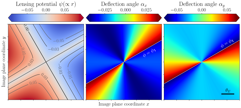
Figure 10: Illustration of the jump discontinuity in deflection angles appearing at the $\phi=\phi_{1}$ line when attempting to symmetrize the $\propto r$ potential for the $m=1$ circular multipole (here, we show an example with $a_{1}=0.1$ and $\phi_{1}=\frac{\pi}{6}$).

A.2 Justifications for the $\propto r\ln r$ potential

A.2.1 Isothermal limit of the non-isothermal solution

The circular multipoles can easily be generalized to non-isothermal slopes [26, 67], i.e., convergence profiles with a radial dependence $\kappa(r)\propto r^{1-\gamma}$ where $\gamma$ is a free parameter ($1<\gamma<3$ for galaxy models, with $\gamma=2$ the isothermal case). Defining $\beta=3-\gamma$, we can use a formalism similar to the one presented in Section II and write the following lensing potential/density pair [26]:

$$\psi(r,\phi)=r^{\beta}F(\phi)\ ;\kappa(r,\phi)=\frac{1}{2}r^{\beta-2}G(\phi)$$ (43)

where the angular shape functions obey the differential equation $G(\phi)=\beta^{2}F(\phi)+F^{\prime\prime}(\phi)$ by virtue of Poisson’s equation.

Circular multipole pertubations have the same shape function for the convergence $G_{m}^{\rm circ}(\phi)$ than in the isothermal case - see Equation (5). The shape function for the potential, however, is different: solving the new differential equation, we find

$$F_{m,\beta}^{\rm circ}(\phi)=\frac{a_{m}^{\rm circ}}{\beta^{2}-m^{2}}\cos(m(\phi-\phi_{m}))+A_{m,\beta}^{\rm circ}\cos(\beta(\phi-\phi_{m}))+B_{m,\beta}^{\rm circ}\sin(\beta(\phi-\phi_{m}))$$ (44)

where $A_{m,\beta}^{\rm circ},B_{m,\beta}^{\rm circ}$ are a priori free constants, since $\cos(\beta\phi)$ and $\sin(\beta\phi)$ verify the homogenous equation. We can use the invariance properties of $G_{m}^{\rm circ}(\phi)$ to determine these constants, by requiring $F_{m,\beta}^{\rm circ}(\phi)$ to have the same symmetries. To begin with, we expect $F_{m,\beta}^{\rm circ}(\phi)$ to be $2\pi$-periodic, implying that terms in $\cos(\beta\phi)$ or $\sin(\beta\phi)$ must vanish unless $0<\beta<2$ is an integer, i.e., unless $\beta=1$. In the $\beta=1$ case, the same conclusion is reached due to invariance under $\phi\mapsto\phi+\pi/(2m)$ for $m\geq 2$, and under any rotation $\phi\mapsto\phi+C$ for $m=0$. In the end, we always have $A_{m,\beta}^{\rm circ}=B_{m,\beta}^{\rm circ}=0$ except for the $m=1,\beta=1$ case, which is treated separately anyways (see Section IV.1). In particular, Equation (19) is naturally recovered from Equation (44) when $\beta=1$ and $m\neq 1$.

We expect that the non-isothermal potentials converge to the isothermal solutions when $\gamma\to 2$ (or equivalently $\beta\to 1$), which is trivially verified for $m\neq 1$. For the $m=1$ case, we write the $\beta\neq 1$ potential in the form:

$$\psi_{m=1,\beta}^{circ}(r,\phi)=r^{\beta}\frac{a_{1}^{\rm circ}}{\beta^{2}-1}\cos(\phi-\phi_{1})+C_{1,\beta}^{\rm circ}r\cos(\phi-\phi_{1})+D_{1,\beta}^{\rm circ}r\sin(\phi-\phi_{1})$$ (45)

where we have introduced two terms with free constants $C_{1,\beta}^{\rm circ},D_{1,\beta}^{\rm circ}$ in order to make the prismatic degeneracy explicit. Since $G_{1}^{\rm circ}(\phi)$ is invariant under $\phi-\phi_{m}\mapsto-(\phi-\phi_{m})$, we need $D_{1,\beta}^{\rm circ}=0$ in order to have the same symmetry in the potential. $C_{1,\beta}^{\rm circ}$ cannot be constrained in a similar fashion, so we leave it free for the moment. Performing a Taylor expansion in the limit $\beta\to 1$, we find:

$$\begin{split}\psi_{m=1,\beta}^{circ}(r,\phi)&\mathrel{\underset{\beta\to 1}{=}}r\Big{(}1+(\beta-1)\ln r+O[(\beta-1)^{2}]\Big{)}\frac{a_{1}^{\rm circ}}{\beta^{2}-1}\cos(\phi-\phi_{1})+C_{1,\beta}^{\rm circ}r\cos(\phi-\phi_{1})\\ &\mathrel{\underset{\beta\to 1}{=}}r\cos(\phi-\phi_{1})\left(\frac{a_{1}^{\rm circ}}{\beta^{2}-1}+C_{1,\beta}^{\rm circ}\right)+\frac{a_{1}^{\rm circ}}{2}r\ln r\cos(\phi-\phi_{1})+O[\beta-1]\end{split}$$ (46)

Therefore, if we want $\psi_{m=1,\beta}^{circ}$ to be convergent, we need to choose $C_{1,\beta}$ such that $\frac{a_{1}^{\rm circ}}{\beta^{2}-1}+C_{1,\beta}$ has a finite limit $L$ when $\beta\to 1$. Then, if we define $r_{E}\equiv\exp\left(-2L/a_{1}^{\rm circ}\right)$, we have:

$$\psi_{m=1,\beta}^{circ}(r,\phi)\mathrel{\underset{\beta\to 1}{\longrightarrow}}\frac{a_{1}^{\rm circ}}{2}r\ln\left(\frac{r}{r_{E}}\right)\cos(\phi-\phi_{1}),$$ (47)

which is precisely the potential $\psi_{1}^{circ}(r,\phi)$ that we have proposed in Equation (21) for the isothermal $m=1$ circular multipole.

We warn that, in current uses [e.g., 67] and implementations of the non-isothermal circular multipoles, the term in $C_{1,\beta}$ is ignored, which would cause the multipole potential (and the deflection angles) to diverge when $\beta\to 1$. In theory, the prismatic degeneracy allows to compensate this by moving the source as much as required, but in practice this would be limited by any priors placed on the source position. To avoid biasing the lens models for near-isothermal slopes, we recommend including this term with an appropriate choice for the constant, for instance:

$$C_{1,\beta}=-a_{1}^{\rm circ}\left(\frac{1}{\beta^{2}-1}+\frac{\ln r_{E}}{2}\right)$$ (48)

with the same choice of normalizing radius $r_{E}$ as for $m=1,\beta=1$ (in our case $r_{E}=\theta_{E}$) in order to ensure the proper convergence.

A.2.2 Direct integration in complex formulation

The gravitational lensing formalism has a complex formulation, introduced by [88, 89], in which the lens equation is written

$$z_{s}=z-\alpha(z)$$ (49)

where complex quantities are used instead their 2D vector equivalent for the position in the source plane $z_{s}=x_{s}+iy_{s}$, the position in the image plane $z=x+iy$, and the deflection angle $\alpha=\alpha_{x}+i\alpha_{y}$ [16]. For a convergence profile $\kappa(z,\overline{z})$ (where $\overline{z}$ denotes the complex conjugate), the complex deflection angle at image position $z_{0}$ can be written [e.g., 90]:

$$\alpha(z_{0})=\frac{1}{\pi}\int_{\mathbb{R}^{2}}\frac{\kappa(z,\overline{z})}{\overline{z}_{0}-\overline{z}}dxdy.$$ (50)

Let us perform this integration with the following convergence profile:

$$\kappa_{1}^{\rm circ}(r,\phi)=\begin{cases}\frac{a_{1}^{\rm circ}\cos\phi}{2r}&\text{ if }r\leq r_{\rm max}\\ 0&\text{ otherwise.}\end{cases}$$ (51)

i.e., a circular $m=1$ multipole profile with $\phi_{1}=0$ that has been truncated beyond some radius $r_{\rm max}$ (otherwise, the integral diverges). Changing to polar coordinates in the integral of Equation (50), we can write:

$$\begin{split}\overline{\alpha_{1}^{\rm circ}}(z_{0})&=\frac{a_{1}^{\rm circ}}{2\pi}\int_{0}^{r_{\rm max}}dr\int_{-\pi}^{\pi}d\phi\frac{\cos\phi}{z_{0}-r\cos\phi-ir\sin\phi}\\ &=\frac{a_{1}^{\rm circ}}{2\pi}\left(\pi\int_{0}^{|z_{0}|}\frac{r}{z_{0}^{2}}dr-\pi\int_{|z_{0}|}^{r_{\rm max}}\frac{dr}{r}\right)\\ &=\frac{a_{1}^{\rm circ}}{2}\ln\left(\frac{|z_{0}|}{r_{\rm max}}\right)+\frac{a_{1}^{\rm circ}}{4}\frac{|z_{0}|^{2}}{z_{0}^{2}}\end{split}$$ (52)

where we have used the following integral:

$$\int_{-\pi}^{\pi}d\phi\frac{\cos\phi}{z_{0}-r\cos\phi-ir\sin\phi}=\begin{cases}-\frac{\pi}{r}\text{ if }r\geq|z_{0}|\\ \frac{r\pi}{z_{0}^{2}}\text{ if }r<|z_{0}|\end{cases}$$ (53)

Then, taking the real/imaginary parts of the complex conjugate of Equation  (52) with $z_{0}=re^{i\phi}$, we find the real-valued deflection angles:

$$\begin{split}\alpha_{x,1}^{\rm circ}(r,\phi)&=\frac{a_{1}^{\rm circ}}{2}\left[\ln\left(\frac{r}{r_{\rm max}}\right)+\cos^{2}\phi+\frac{1}{2}\right]\\ \alpha_{y,1}^{\rm circ}(r,\phi)&=\frac{a_{1}^{\rm circ}}{2}\cos\phi\sin\phi\end{split}$$ (54)

which match Equation (22) with $\phi_{1}=0$, up to a constant $\frac{1}{2}+\ln\left(\frac{r_{\rm max}}{r_{E}}\right)$ for $\alpha_{x}$. Thanks to the prismatic degeneracy, we can add any constant to the deflection field without impacting the lensing observables, so these solutions are equivalent, even as we take $r_{\rm max}\to\infty$. The more general solution with $\phi_{1}$ free can be deduced from the $\phi_{1}=0$ case by a simple rotation of the coordinate system.

Appendix B General solutions for the lensing potential of the elliptical multipoles

In this section, we present the lensing potential solutions for the elliptical multipoles of general order $m\geq 2$, separating the cases where $m$ is odd (Appendix B.1) and $m$ is even (Appendix B.2). This is mostly done for completeness: the solutions for the $m=3$ and $m=4$ orders were presented in Sections IV.3 and IV.4 in equivalent, “simplified” forms, better suited for pratical applications.

B.1 Lensing potential for elliptical multipoles with $m$ odd

In this section, we assume that $m\geq 3$ is odd, i.e., that we can write $m=2k+1$ for $k\in\mathbb{N}^{*}$. We have the following explicit expression for the Chebyshev polynomials of the first kind:

$$T_{m}(x)=\frac{m}{2}\sum_{p=0}^{\lfloor m/2\rfloor}\left(-1\right)^{p}\frac{(m-p-1)!}{p!(m-2p)!}(2x)^{m-2p}=\frac{m}{2}\sum_{l=0}^{k}\left(-1\right)^{k-l}\frac{1}{k+l+1}\binom{k+l+1}{2l+1}(2x)^{2l+1}$$ (55)

where, in the second sum, we have made the change of variables $l=k-p$. Plugging this into Equation (12), we find that we can write the shape function as a linear combination of simpler functions:

$$G_{m}^{(1)}(\phi;q)=\sum_{l=0}^{+\infty}g_{kl}(q)\cdot u_{l}(\phi;q)$$ (56)

where we have defined

$$\begin{split}u_{l}(\phi;q)&\equiv\frac{\cos^{2l+1}\phi}{(q^{2}\cos^{2}\phi+\sin^{2}\phi)^{l+1}}\text{ for $l\in\mathbb{R}$}\\ \text{and }g_{kl}(q)&\equiv\begin{cases}(-1)^{k-l}\frac{2k+1}{2(k+l+1)}\binom{k+l+1}{2l+1}(2q)^{2l+1}\text{ if }l\leq k\\ 0\text{ otherwise }\end{cases}\end{split}$$ (57)

The (unsymmetrized) solution to differential Equation (2) has the following form:

$$\begin{split}\tilde{F}_{m}^{(1)}(\phi;q)=\frac{1}{(1-q^{2})^{k+1}}\Bigg{[}&A_{m}^{(1)}(q)\cos\phi+B_{m}^{(1)}(q)\sin\phi+C_{m}^{(1)}(q)\mathscr{C}(\phi;q)\\ &+D_{m}^{(1)}(q)\mathscr{D}(\phi;q)+\sum_{j=1}^{k-1}\xi_{mj}^{(1)}(q)u_{j-1}(\phi;q)\Bigg{]}\end{split}$$ (58)

where the coefficients $A_{m}^{(1)},B_{m}^{(1)},C_{m}^{(1)},D_{m}^{(1)},\{\xi_{mj}^{(1)}\}$ are functions of $q$ only (i.e., independent of $\phi$), and we have defined:

$$\begin{split}\mathscr{C}(\phi;q)&=\cos(\phi)\ln\left[1+q^{2}+(q^{2}-1)\cos(2\phi)\right]+2\phi\sin\phi\\ \mathscr{D}(\phi;q)&=\sin(\phi)\varphi(\phi;q)\end{split}$$ (59)

To determine the coefficients, we write the derivatives as combinations of the functions $u_{l}$ defined above:

$$\begin{split}\mathscr{C}^{\prime\prime}(\phi;q)+\mathscr{C}(\phi;q)=&\frac{2(1-q^{2})}{(q^{2}\cos^{2}\phi+\sin^{2}\phi)^{2}}\left[-2(1-q^{2})\cos^{5}\phi+(5-q^{2})\cos^{3}\phi-3\cos\phi\right]+4\cos\phi\\ =&-2(1-3q^{2})u_{0}+4q^{2}(1-q^{2})u_{1}\hfill\\ \mathscr{D}^{\prime\prime}(\phi;q)+\mathscr{D}(\phi;q)=&\frac{q^{3}\cos\phi}{(q^{2}\cos^{2}\phi+\sin^{2}\phi)^{2}}\\ =&\ 2q^{3}u_{0}+2q^{3}(1-q^{2})u_{1}\\ u_{j-1}^{\prime\prime}(\phi;q)+u_{j-1}(\phi;q)=&\Big{[}(q^{4}-jq^{2})\cos^{4}\phi+(j(2j+1)+q^{2}(2-5j))\cos^{2}\phi\sin^{2}\phi\\ &+2(j-1)(2j-1)\sin^{4}\phi\Big{]}\frac{2\cos^{2j-3}\phi}{(q^{2}\cos^{2}\phi+\sin^{2}\phi)^{j+2}}\\ =&\ 2(j-1)(2j-1)u_{j-2}+\left[2(1-q^{2})(2j(3j-2)+1)-4j(j-1)\right]u_{j-1}\\ &+\left[-8j^{2}(1-q^{2})+2(1-q^{2})^{2}j(6j+1)\right]u_{j}-4j(j+1)q^{2}(1-q^{2})^{2}u_{j+1}\end{split}$$ (60)

We can then write, with the convention $\xi_{mj}^{(1)}=0$ if $j\geq k$ or $j\leq 0$:

$$\begin{split}(1-&q^{2})^{k+1}\left[\tilde{F}_{m}^{(1)\prime\prime}(\phi;q)+\tilde{F}_{m}^{(1)}(\phi;q)\right]\\ =&\left[-2(1-3q^{2})C_{m}^{(1)}+2q^{3}D_{m}^{(1)}\right]u_{0}+\left[4q^{2}(1-q^{2})C_{m}^{(1)}+2q^{3}(1-q^{2})D_{m}^{(1)}\right]u_{1}\\ &\begin{split}+\sum_{j=0}^{k+1}&\left\{-4j(j-1)q^{2}(1-q^{2})^{2}\xi_{m(j-1)}^{(1)}+\left[-8j^{2}(1-q^{2})+2(1-q^{2})^{2}j(6j+1)\right]\xi_{mj}^{(1)}\right.\\ +&\left.\left[2(1-q^{2})(2(j+1)(3j+1)+1)-4j(j+1)\right]\xi_{m(j+1)}^{(1)}+2(j+1)(2j+3)\xi_{m(j+2)}^{(1)}\right\}u_{j}\end{split}\end{split}$$ (61)

In order for $\tilde{F}_{m}^{(1)}(\phi;q)$ to be a solution of the differential Equation (2), it is sufficient to match the coefficients in front of the $u_{j}$ in Equations (56) and (61). This amounts to solving a matrix–vector equation:

$$M_{m}(q)\cdot\begin{pmatrix}C_{m}^{(1)}\\ D_{m}^{(1)}\\ \xi_{m1}^{(1)}\\ \vdots\\ \xi_{m(k-1)}^{(1)}\end{pmatrix}=(1-q^{2})^{k+1}\begin{pmatrix}g_{k0}\\ g_{k1}\\ \vdots\\ g_{kk}\end{pmatrix}$$ (62)

The $(k+1)\times(k+1)$ matrix $M_{m}(q)$ can be written in a block-triangular form:

$$M_{m}(q)=\begin{pmatrix}M_{m}^{\rm sup}(q)&M_{m}^{\rm ur}(q)\\ (0)&M_{m}^{\rm tri}(q)\end{pmatrix}$$ (63)

where $M_{m}^{\rm sup}(q)=\begin{pmatrix}-2(1-3q^{2})&2q^{3}\\ 4q^{2}(1-q^{2})&2q^{3}(1-q^{2})\end{pmatrix}$ and the two other blocks $M_{m}^{\rm ur}(q),M_{m}^{\rm tri}(q)$ are determined by:

$$\begin{split}\quad M_{m}(q)[j,j+3]&=2(j+1)(2j+3)\text{ if }0\leq j\leq k-3,\\ \quad M_{m}(q)[j,j+2]&=2(1-q^{2})\left(2(j+1)(3j+1)+1\right)-4j(j+1)\text{ if }0\leq j\leq k-2,\\ \quad M_{m}(q)[j,j+1]&=-8j^{2}(1-q^{2})+2(1-q^{2})^{2}j(6j+1)\text{ if }1\leq j\leq k-1,\\ \quad M_{m}(q)[j,j]&=-4j(j-1)q^{2}(1-q^{2})^{2}\text{ if }2\leq j\leq k,\end{split}$$ (64)

all the other coefficients being zero.

As a consequence, the lower-right block $M_{m}^{\rm tri}$ is upper triangular and we can easily write the determinant of $M_{m}$:

$$\begin{split}\det\left[M_{m}(q)\right]&=\det\left[M_{m}^{\rm sup}(q)\right]\times\det\left[M_{m}^{\rm tri}(q)\right]\\ &=-4q^{3}(1-q^{2})^{2}\times\prod_{j=2}^{k}-4j(j-1)q^{2}(1-q^{2})^{2}\\ &=q^{2k+1}(2(1-q^{2}))^{2k}k!(k-1)!\end{split}$$ (65)

Since $\det\left[M_{m}(q)\right]\neq 0$ for $q\neq 1$ ( $q=1$ corresponding to the circular multipole solution), Equation (62) always has a solution when relevant and the coefficients $C_{m}^{(1)},D_{m}^{(1)},E_{m}^{(1)},\{\xi_{mj}^{(1)}\}$ are fully determined.

We have therefore solved differential Equation (2) for $G_{m}^{(1)}(\phi;q)$ - the remaining coefficients $A_{m}^{(1)}$ and $B_{m}^{(1)}$ only correspond to the terms of the homogeneous equation, and once again, they do not matter for the lensing observables due to the prismatic degeneracy (see Section II or [59]). However, the solution $\tilde{F}_{m}^{(1)}(\phi;q)$ does not have all expected symmetries: choosing $B_{m}^{(1)}=0$, we enforce the $\phi\mapsto-\phi$ symmetry ; but Equation (58) cannot be made $2\pi$-periodic or $\phi\mapsto\pi-\phi$ antisymmetric, because of the terms in $\phi\sin\phi$ and $\sin(\phi)\varphi(\phi;q)$. Direct symmetrization of the shape function leads to jump discontinuties in the deflection field, like in Sections IV.1, IV.2, and IV.3 ; so we use the same trick as before, dividing the lensing potential into two components:

$$\psi_{m}^{(1)}(r,\phi;q)=r\hat{F}_{m}^{(1)}(\phi;q)+\lambda_{m}(q)\cdot\psi_{1}^{\rm circ}\left(r,\phi\right)\Big{|}_{\phi_{1}=0,a_{1}^{\rm circ}=1}$$ (66)

where we have defined

$$\begin{split}\hat{F}_{m}^{(1)}(\phi;q)&=\tilde{F}_{m}^{(1)}(\phi;q)-\frac{\lambda_{m}(q)}{2}\phi\sin\phi\\ &=\tilde{F}_{m}^{(1)}(\phi;q)-\lambda_{m}(q)\cdot\tilde{F}_{m}^{\rm circ}(\phi)\Big{|}_{\phi_{1}=0,a_{1}^{\rm circ}=1}\end{split}$$ (67)

This modified shape function $\hat{F}_{m}^{(1)}(\phi;q)$ can have the correct symmetries ($2\pi$ periodic, symmetric under $\phi\mapsto-\phi$ and antisymmetric under $\phi\mapsto\pi-\phi$): we simply need to choose $\lambda_{m}(q)$ so that terms in $\phi$ and $\varphi(\phi,q)$ can be factorized as $\phi-\varphi(\phi,q)$ (see Section IV.2). Examining the coefficients in Equation (58) and (59), we obtain the following condition:

$$\lambda_{m}(q)=\frac{2D_{m}^{(1)}(q)+4C_{m}^{(1)}(q)}{(1-q^{2})^{k+1}}$$ (68)

In practice, we find that the following expression is verified at least for $1\leq k<10$:

$$\lambda_{m}(q)=\frac{2(q-1)^{k}}{(q+1)^{k+1}}\mathrel{\underset{q\to 1}{\longrightarrow}}0.$$ (69)

We saw that $B_{m}^{(1)}(q)=0$ was imposed from the expected symmetries, but the other remaining coefficient $A_{m}^{(1)}(q)$ cannot be determined in such manner. Instead, using a similar approach to the $m=3$ case (see Section IV.3), we write the Taylor expansion of $\tilde{F}_{m}^{(1)}(\phi;q)$ when $q\to 1$ for $\phi=0$:

$$\tilde{F}_{m}^{(1)}(\phi=0;q)\mathrel{\underset{q\to 1}{=}}\frac{A_{m}^{(1)}}{(1-q^{2})^{k+1}}+\sum_{j=0}^{k+1}\frac{t_{mj}}{(1-q)^{j}}+O[1-q]$$ (70)

where the $t_{mj}$ can be determined with a symbolic calculator. Assuming that we indeed have $\lambda_{m}(q)\mathrel{\underset{q\to 1}{\longrightarrow}}0$, the potential $\psi_{m}^{(1)}$ will converge to the circular multipole solution in the limit $q\to 1$ if $\tilde{F_{m}}^{(1)}(\phi;q)\mathrel{\underset{q\to 1}{\longrightarrow}}F_{m}^{\rm circ}(\phi)\Big{|}_{\phi_{m}=0,a_{m}^{\rm circ}=1}$. This is ensured if we choose

$$A_{m}^{(1)}(q)=(1-q^{2})^{k+1}\left[\frac{1}{1-m^{2}}-\sum_{j=0}^{k+1}\frac{t_{mj}}{(1-q)^{j}}\right].$$ (71)

We could add any term $f(q)$ to $A_{m}^{(1)}$ as long as $f(q)(1-q)^{-(k+1)}\mathrel{\underset{q\to 1}{\longrightarrow}}0$, but thanks to the prismatic degeneracy, this would not change the lensing observables, so we can safely ignore it and choose $f(q)=0$ for simplicity.

We note that, following the method described in this section, we obtain the following coefficients: $C_{3}^{(1)}(q)=\frac{1}{2}q(3+q^{2})$, $D_{3}^{(1)}(q)=-(1+3q^{2})$ and $A_{3}^{(1)}(q)$ given by Equation (34). Accordingly, one can easily check that we recover the same solution for the $m=3$ lensing potential as in Section IV.3.

Now that $\psi_{m}^{(1)}(\phi;q)$ is fully formulated, the other component $\psi_{m}^{(2)}(\phi;q)$ can be determined without additional effort, by making use of Equation (17). This completes the description of the elliptical multipole lensing potential in the general $m=2k+1$ case. In Figure 11, we show example potential maps for the $m=5$ elliptical multipole calculated using the method described in this Appendix, as well as the effect of such a perturbation on a SIE convergence profile, in comparison with the $m=5$ circular multipole.

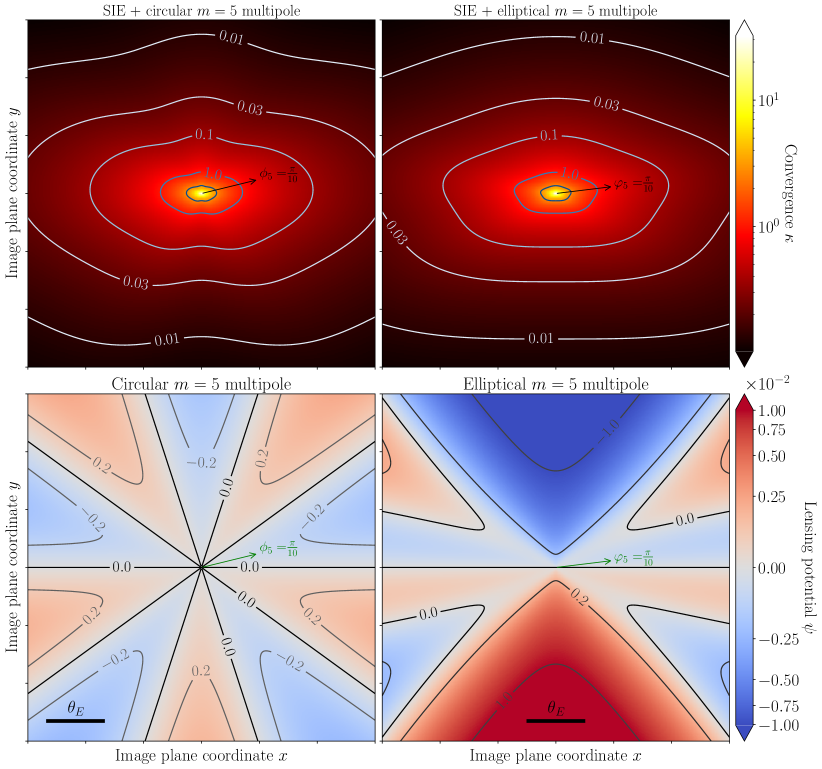
Figure 11: Top panel: Impact of a $m=5$ multipole on the convergence profile of a SIE lens model with axis ratio $q=0.5$, in the circular (left) and elliptical (right) formulations. We choose perturbations with direction $\phi_{5}=\frac{\pi}{10}$ (resp. $\varphi_{1}=\frac{\pi}{10}$) amplitude $a_{1}^{\rm circ}=0.027$ (resp. $a_{1}=0.027$). Bottom panel: lensing potentials corresponding to the $m=5$ multipole term only.

B.2 Lensing potential for elliptical multipoles with $m$ even

In this section, we assume that $m\geq 2$ is even, i.e., that we can write $m=2k$ for $k\in\mathbb{N}^{*}$. The Chebyshev polynomials of the first and second kind can be written explicitely as:

$$\begin{split}T_{m}(x)&=\frac{m}{2}\sum_{p=0}^{\lfloor m/2\rfloor}\left(-1\right)^{p}\frac{(m-p-1)!}{p!(m-2p)!}(2x)^{m-2p}=k\sum_{l=0}^{k}\left(-1\right)^{k-l}\frac{k}{k+l}\binom{k+l}{k-l}(2x)^{2l}\\ U_{m-1}(x)&=\sum_{p=0}^{\lfloor\frac{m-1}{2}\rfloor}\left(-1\right)^{p}\binom{m-1-p}{p}(2x)^{m-1-2p}=\sum_{l=0}^{k-1}\left(-1\right)^{k-l-1}\binom{k+l}{k-l-1}(2x)^{2l+1}\end{split}$$ (72)

where we have made the change of variables $l=k-p$ in the first line, and $l=k-1-p$ in the second line. Again, plugging this into Equation (12), we write the shape functions as a linear combination of basis functions:

$$\begin{split}G_{m}^{(1)}(\phi;q)&=\sum_{l=0}^{+\infty}\gamma_{kl}^{(1)}(q)\cdot u_{l-1/2}(\phi;q)\\ G_{m}^{(2)}(\phi;q)&=\sum_{l=0}^{+\infty}\gamma_{kl}^{(2)}(q)\cdot w_{l}(\phi;q)\end{split}$$ (73)

where we use the same definition for $u_{l}$ as in Section B.1 such that $u_{l-1/2}(\phi;q)=\frac{\cos^{2l}\phi}{(q^{2}\cos^{2}\phi+\sin^{2}\phi)^{l+1/2}}$, and we define $w_{l}(\phi;q)\equiv\frac{\sin\phi\cos^{2l+1}\phi}{(q^{2}\cos^{2}\phi+\sin^{2}\phi)^{l+3/2}}$, as well as the coefficients

$$\begin{split}\gamma_{kl}^{(1)}(q)&\equiv\begin{cases}\left(-1\right)^{k-l}\frac{k}{k+l}\binom{k+l}{k-l}(2q)^{2l}\text{ if }l\leq k\\ 0\text{ otherwise }\end{cases}\\ \text{ and }\gamma_{kl}^{(2)}(q)&\equiv\begin{cases}\left(-1\right)^{k-l-1}\binom{k+l}{k-l-1}(2q)^{2l+1}\text{ if }l\leq k-1\\ 0\text{ otherwise }\end{cases}\end{split}$$ (74)

The solutions to differential Equation (2) have the following form:

$$\begin{split}F_{m}^{(1)}(\phi;q)&=\frac{1}{(1-q^{2})^{k+1/2}}\Bigg{[}A_{m}^{(1)}(q)\cos\phi+B_{m}^{(1)}(q)\sin\phi+E_{m}^{(1)}(q)\mathscr{E}_{1}(\phi;q)+\sum_{j=0}^{k-1}\lambda_{mj}^{(1)}(q)v_{j}^{(1)}(\phi;q)\Bigg{]}\\ F_{m}^{(2)}(\phi;q)&=\frac{1}{(1-q^{2})^{k+1/2}}\Bigg{[}A_{m}^{(2)}(q)\cos\phi+B_{m}^{(2)}(q)\sin\phi+E_{m}^{(2)}(q)\mathscr{E}_{2}(\phi;q)+\sum_{j=0}^{k-1}\lambda_{mj}^{(2)}(q)v_{j}^{(2)}(\phi;q)\Bigg{]}\end{split}$$ (75)

where the coefficients $A_{m}^{(i)},B_{m}^{(i)},E_{m}^{(i)},\{\lambda_{mj}^{(i)}\}$ are functions of $q$ only (i.e., independent of $\phi$), and we have defined:

$$\begin{split}\mathscr{E}_{1}(\phi;q)=&+\cos(\phi)\arctan\left(\frac{\sqrt{(1-q^{2})}\cos(\phi)}{\sqrt{q^{2}\cos^{2}\phi+\sin^{2}\phi}}\right)\\ &+\sin(\phi)\log\left(\frac{\sqrt{1-q^{2}}\sin(\phi)}{q}+\sqrt{1+\frac{(1-q^{2})}{q^{2}}\sin^{2}(\phi)}\right)\\ \mathscr{E}_{2}(\phi;q)=&-\sin(\phi)\arctan\left(\frac{\sqrt{(1-q^{2})}\cos(\phi)}{\sqrt{q^{2}\cos^{2}\phi+\sin^{2}\phi}}\right)\\ &+\cos(\phi)\log\left(\frac{\sqrt{1-q^{2}}\sin(\phi)}{q}+\sqrt{1+\frac{(1-q^{2})}{q^{2}}\sin^{2}(\phi)}\right)\\ v_{j}^{(1)}(\phi;q)=&\cos^{2}(\phi)u_{j-3/2}(\phi;q)=\frac{\cos^{2j}\phi}{(q^{2}\cos^{2}\phi+\sin^{2}\phi)^{j-1/2}}\\ v_{j}^{(2)}(\phi;q)=&\cos(\phi)\sin(\phi)u_{j-1/2}(\phi;q)=\frac{\sin\phi\cos^{2j+1}\phi}{(q^{2}\cos^{2}\phi+\sin^{2}\phi)^{j+1/2}}=(q^{2}\cos^{2}\phi+\sin^{2}\phi)w_{j}(\phi;q)\end{split}$$ (76)

The expressions in Equation (75) are $2\pi$-periodic, and, if (and only if) we choose $A_{m}^{(1)}=B_{m}^{(1)}=A_{m}^{(2)}=B_{m}^{(2)}=0$, they already have the expected symmetries: $F_{m}^{(1)}$ (resp. $F_{m}^{(2)}$) is symmetric (resp. antisymmetric) under $\phi\mapsto-\phi$ and $\phi\mapsto\pi-\phi$.To determine the remaining coefficients, we follow the same approach as in Section B.1, and express the derivatives as linear combinations of the same basis functions used to describe $G_{m}^{(1)}$ and $G_{m}^{(2)}$:

$$\begin{split}\mathscr{E}_{1}^{\prime\prime}(\phi;q)+\mathscr{E}_{1}(\phi;q)&=\sqrt{1-q^{2}}\ u_{-1/2}\\ v_{j}^{(1)\prime\prime}(\phi;q)+v_{j}^{(1)}(\phi;q)&=(2j-1)\left[2ju_{j-3/2}+(2j-(4j+1)q^{2})u_{j-1/2}-(2j+1)q^{2}(1-q^{2})u_{j+1/2}\right]\\ \mathscr{E}_{2}^{\prime\prime}(\phi;q)+\mathscr{E}_{2}(\phi;q)&=-(1-q^{2})^{3/2}\ w_{0}\\ v_{j}^{(2)\prime\prime}(\phi;q)+v_{j}^{(2)}(\phi;q)&=(2j+1)\left[2jw_{j-1}+(2j-(4j+3)q^{2})w_{j}-(2j+3)q^{2}(1-q^{2})w_{j+1}\right]\\ \end{split}$$ (77)

We can then express $F_{m}^{(i)\prime\prime}+F_{m}^{(i)}$ as a function of the $u_{j-1/2}$ (for i=1) or the $w_{j}$ (for $i=2$), and match the coefficients to those found in Equation (73). This results in two matrix-vector equations:

$$N_{m}^{(1)}(q)\cdot\begin{pmatrix}E_{m}^{(1)}\\ \lambda_{m0}^{(1)}\\ \vdots\\ \lambda_{m(k-1)}^{(1)}\end{pmatrix}=(1-q^{2})^{k+1/2}\begin{pmatrix}\gamma_{k0}^{(1)}\\ \gamma_{k1}^{(1)}\\ \vdots\\ \gamma_{kk}^{(1)}\end{pmatrix};\text{ and }N_{m}^{(2)}(q)\cdot\begin{pmatrix}E_{m}^{(2)}\\ \lambda_{m0}^{(2)}\\ \vdots\\ \lambda_{m(k-2)}^{(2)}\end{pmatrix}=(1-q^{2})^{k+1/2}\begin{pmatrix}\gamma_{k0}^{(2)}\\ \gamma_{k1}^{(2)}\\ \vdots\\ \gamma_{k(k-1)}^{(2)}\end{pmatrix}$$ (78)

where the matrices $N_{m}^{(1)}(q)$ and $N_{m}^{(2)}(q)$, respectively of dimension $(k+1)\times(k+1)$ and $k\times k$, with their only non-zero coefficients being:

$$\begin{split}\quad N_{m}^{(1)}(q)[j,j]&=\begin{cases}\sqrt{1-q^{2}}\text{ if }j=0\\ -(2j-3)(2j-1)q^{2}(1-q^{2})\text{ if }1\leq j\leq k\end{cases}\\ \quad N_{m}^{(1)}(q)[j,j+1]&=(2j-1)\left[2j-(4j+1)q^{2}\right]\text{ if }0\leq j\leq k-1,\\ \quad N_{m}^{(1)}(q)[j,j+2]&=2(j+1)(2j+1)\text{ if }0\leq j\leq k-2,\\ \quad N_{m}^{(2)}(q)[j,j]&=\begin{cases}-(1-q^{2})^{3/2}\text{ if }j=0\\ -(2j-1)(2j+1)q^{2}(1-q^{2})\text{ if }1\leq j\leq k\end{cases}\\ \quad N_{m}^{(2)}(q)[j,j+1]&=(2j+1)\left[2j-(4j+3)q^{2}\right]\text{ if }0\leq j\leq k-1,\\ \quad N_{m}^{(2)}(q)[j,j+2]&=2(j+1)(2j+3)\text{ if }0\leq j\leq k-2,\\ \end{split}$$ (79)

We note that $N_{m}^{(1)}(q)$ and $N_{m}^{(2)}(q)$ are upper triangular, and for $0<q<1$ they have only non-zero diagonal coefficients, so Equation (78) always has a solution, and thus, all the coefficients are determined. For the $m=4$, the equations above yield:

$$E_{4}^{(1)} =1+6q^{2}+q^{4}, \lambda_{4,0}^{(1)} =-\frac{8}{3}(1+2q^{2})\sqrt{1-q^{2}}, \lambda_{4,1}^{(1)} =-\frac{8}{3}q^{2}(1-q^{2})^{3/2},$$

$$E_{4}^{(2)} =4q(1+q^{2}), \lambda_{4,0}^{(2)} =-\frac{8}{3}q(1-q^{2})^{3/2},$$ (80)

and by plugging these coefficients into Equation (75), we recover the same shape functions as in Section IV.4.

The lensing potential is then straightforwardly calculated: since the shape functions already have the right symmetries, there is no need to decompose the potential like in the odd $m$ case. Furthermore, we verified numerically for $1\leq k<7$ that the shape functions written in Equation (75) converged to the circular multipole solution when $q\to 1$. Thus, we simply need to plug the expressions for $F_{m}^{(1)}$ and $F_{4}^{(2)}$ in Equation (14), then apply Equation (1) with the resulting shape function $F_{m}(\phi;q)$. This completes the description of the elliptical multipole lensing potential in the general $m=2k$ case. In Figure 12, we show example potential maps for the $m=6$ elliptical multipole calculated using the method described in this Appendix, as well as the effect of such a perturbation on a SIE convergence profile, in comparison with the $m=6$ circular multipole.

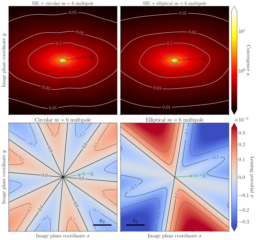
Figure 12: Same as Figure 11, but for a $m=6$ multipole with direction $\phi_{6}=\frac{\pi}{18}$ (resp. $\varphi_{6}=\frac{\pi}{18}$), and amplitude $a_{4}^{\rm circ}=0.015$ (resp. $a_{4}=0.015$).

References

- Wong et al. [2020] K. C. Wong, S. H. Suyu, G. C. F. Chen, C. E. Rusu, M. Millon, D. Sluse, V. Bonvin, C. D. Fassnacht, S. Taubenberger, M. W. Auger, S. Birrer, J. H. H. Chan, F. Courbin, S. Hilbert, O. Tihhonova, T. Treu, A. Agnello, X. Ding, I. Jee, E. Komatsu, A. J. Shajib, A. Sonnenfeld, R. D. Blandford, L. V. E. Koopmans, P. J. Marshall, and G. Meylan, Mon. Not. Roy. Astron. Soc. 498, 1420 (2020).
- Birrer et al. [2020] S. Birrer, A. J. Shajib, A. Galan, M. Millon, T. Treu, A. Agnello, M. Auger, G. C. F. Chen, L. Christensen, T. Collett, F. Courbin, C. D. Fassnacht, L. V. E. Koopmans, P. J. Marshall, J. W. Park, C. E. Rusu, D. Sluse, C. Spiniello, S. H. Suyu, S. Wagner-Carena, K. C. Wong, M. Barnabè, A. S. Bolton, O. Czoske, X. Ding, J. A. Frieman, and L. Van de Vyvere, Astron. & Astrophys. 643, A165 (2020).
- Hsueh et al. [2020] J. W. Hsueh, W. Enzi, S. Vegetti, M. W. Auger, C. D. Fassnacht, G. Despali, L. V. E. Koopmans, and J. P. McKean, Mon. Not. Roy. Astron. Soc. 492, 3047 (2020).
- Gilman et al. [2020] D. Gilman, S. Birrer, A. Nierenberg, T. Treu, X. Du, and A. Benson, Mon. Not. Roy. Astron. Soc. 491, 6077 (2020).
- Gilman et al. [2023] D. Gilman, Y.-M. Zhong, and J. Bovy, Phys. Rev. D 107, 103008 (2023).
- Treu and Marshall [2016] T. Treu and P. J. Marshall, Ann. Rev. Astron. Astrophys. 24, 11 (2016).
- Treu et al. [2022] T. Treu, S. H. Suyu, and P. J. Marshall, Astron. Astrophys. Rev. 30, 8 (2022).
- Vegetti et al. [2012] S. Vegetti, D. J. Lagattuta, J. P. McKean, M. W. Auger, C. D. Fassnacht, and L. V. E. Koopmans, Nature 481, 341 (2012).
- Shajib et al. [2022] A. J. Shajib, K. C. Wong, S. Birrer, S. H. Suyu, T. Treu, E. J. Buckley-Geer, H. Lin, C. E. Rusu, J. Poh, A. Palmese, A. Agnello, M. W. Auger-Williams, A. Galan, S. Schuldt, D. Sluse, F. Courbin, J. Frieman, and M. Millon, Astron. & Astrophys. 667, A123 (2022).
- Gilman et al. [2024] D. Gilman, S. Birrer, A. Nierenberg, and M. S. H. Oh, Mon. Not. Roy. Astron. Soc. 533, 1687 (2024).
- Turner et al. [1984] E. L. Turner, J. P. Ostriker, and J. R. Gott, III, Astrophys. J. 284, 1 (1984).
- Chae [2003] K.-H. Chae, Mon. Not. Roy. Astron. Soc. 346, 746 (2003).
- Yoo et al. [2005] J. Yoo, C. S. Kochanek, E. E. Falco, and B. A. McLeod, Astrophys. J. 626, 51 (2005).
- Schneider et al. [2006] P. Schneider, G. Meylan, C. Kochanek, P. Jetzer, P. North, and J. Wambsganss, Gravitational Lensing: Strong, Weak and Micro: Saas-Fee Advanced Course 33, Saas-Fee Advanced Course (Springer Berlin Heidelberg, 2006).
- Auger et al. [2009] M. W. Auger, T. Treu, A. S. Bolton, R. Gavazzi, L. V. E. Koopmans, P. J. Marshall, K. Bundy, and L. A. Moustakas, Astrophys. J. 705, 1099 (2009).
- Tessore and Metcalf [2015] N. Tessore and R. B. Metcalf, Astron. & Astrophys. 580, A79 (2015).
- Kassiola and Kovner [1993] A. Kassiola and I. Kovner, Astrophys. J. 417, 450 (1993).
- Kormann et al. [1994a] R. Kormann, P. Schneider, and M. Bartelmann, Astron. & Astrophys. 284, 285 (1994a).
- Kormann et al. [1994b] R. Kormann, P. Schneider, and M. Bartelmann, Astron. & Astrophys. 286, 357 (1994b).
- Keeton et al. [1997] C. R. Keeton, C. S. Kochanek, and U. Seljak, Astrophys. J. 482, 604 (1997).
- Witt and Mao [1997] H. J. Witt and S. Mao, Mon. Not. Roy. Astron. Soc. 291, 211 (1997).
- Hilbert et al. [2007] S. Hilbert, S. D. M. White, J. Hartlap, and P. Schneider, Mon. Not. Roy. Astron. Soc. 382, 121 (2007).
- Moustakas et al. [2007] L. A. Moustakas, P. Marshall, J. A. Newman, A. L. Coil, M. C. Cooper, M. Davis, C. D. Fassnacht, P. Guhathakurta, A. Hopkins, A. Koekemoer, N. P. Konidaris, J. M. Lotz, and C. N. A. Willmer, Astrophys. J. 660, L31 (2007).
- Wong et al. [2011] K. C. Wong, C. R. Keeton, K. A. Williams, I. G. Momcheva, and A. I. Zabludoff, Astrophys. J. 726, 84 (2011).
- Etherington et al. [2024] A. Etherington, J. W. Nightingale, R. Massey, S.-I. Tam, X. Cao, A. Niemiec, Q. He, A. Robertson, R. Li, A. Amvrosiadis, S. Cole, J. M. Diego, C. S. Frenk, B. L. Frye, D. Harvey, M. Jauzac, A. M. Koekemoer, D. J. Lagattuta, S. Lange, M. Limousin, G. Mahler, E. Sirks, and C. L. Steinhardt, Mon. Not. Roy. Astron. Soc. 531, 3684 (2024).
- Evans and Witt [2003] N. W. Evans and H. J. Witt, Mon. Not. Roy. Astron. Soc. 345, 1351 (2003).
- Congdon and Keeton [2005] A. B. Congdon and C. R. Keeton, Mon. Not. Roy. Astron. Soc. 364, 1459 (2005).
- Gomer and Williams [2018] M. R. Gomer and L. L. R. Williams, Mon. Not. Roy. Astron. Soc. 475, 1987 (2018).
- Gilman et al. [2021] D. Gilman, J. Bovy, T. Treu, A. Nierenberg, S. Birrer, A. Benson, and O. Sameie, Mon. Not. Roy. Astron. Soc. 507, 2432 (2021).
- Oh et al. [2024] M. S. H. Oh, A. Nierenberg, D. Gilman, and S. Birrer, arXiv e-prints (2024), arXiv:2404.17124 [astro-ph.CO] .
- Cohen et al. [2024] J. S. Cohen, C. D. Fassnacht, C. M. O’Riordan, and S. Vegetti, Mon. Not. Roy. Astron. Soc. 531, 3431 (2024).
- Keeley et al. [2024] R. E. Keeley, A. M. Nierenberg, D. Gilman, C. Gannon, S. Birrer, T. Treu, A. J. Benson, X. Du, K. N. Abazajian, T. Anguita, V. N. Bennert, S. G. Djorgovski, K. K. Gupta, S. F. Hoenig, A. Kusenko, C. Lemon, M. Malkan, V. Motta, L. A. Moustakas, M. S. H. Oh, D. Sluse, D. Stern, and R. H. Wechsler, Mon. Not. Roy. Astron. Soc. 535, 1652 (2024).
- Carter [1978] D. Carter, Mon. Not. Roy. Astron. Soc. 182, 797 (1978).
- Bender et al. [1987] R. Bender, S. Doebereiner, and C. Moellenhoff, Astron. & Astrophys. 177, L53 (1987).
- Bender et al. [1988] R. Bender, S. Doebereiner, and C. Moellenhoff, Astron. & Astrophys. Suppl. Ser. 74, 385 (1988).
- Hao et al. [2006] C. N. Hao, S. Mao, Z. G. Deng, X. Y. Xia, and H. Wu, Mon. Not. Roy. Astron. Soc. 370, 1339 (2006).
- Kormendy et al. [2009] J. Kormendy, D. B. Fisher, M. E. Cornell, and R. Bender, Astrophys. J. Suppl. 182, 216 (2009).
- Chaware et al. [2014] L. Chaware, R. Cannon, A. K. Kembhavi, A. Mahabal, and S. K. Pandey, Astrophys. J. 787, 102 (2014).
- Cappellari [2016] M. Cappellari, Ann. Rev. Astron. Astrophys. 54, 597 (2016).
- Van de Vyvere et al. [2022a] L. Van de Vyvere, M. R. Gomer, D. Sluse, D. Xu, S. Birrer, A. Galan, and G. Vernardos, Astron. & Astrophys. 659, A127 (2022a).
- Nightingale et al. [2024] J. W. Nightingale, Q. He, X. Cao, A. Amvrosiadis, A. Etherington, C. S. Frenk, R. G. Hayes, A. Robertson, S. Cole, S. Lange, R. Li, and R. Massey, Mon. Not. Roy. Astron. Soc. 527, 10480 (2024).
- O’Riordan and Vegetti [2024] C. M. O’Riordan and S. Vegetti, Mon. Not. Roy. Astron. Soc. 528, 1757 (2024).
- Ciambur [2015] B. C. Ciambur, Astrophys. J. 810, 120 (2015).
- Ciambur and Graham [2016] B. C. Ciambur and A. W. Graham, Mon. Not. Roy. Astron. Soc. 459, 1276 (2016).
- Jedrzejewski [1987] R. I. Jedrzejewski, Mon. Not. Roy. Astron. Soc. 226, 747 (1987).
- Goullaud et al. [2018] C. F. Goullaud, J. B. Jensen, J. P. Blakeslee, C.-P. Ma, J. E. Greene, and J. Thomas, Astrophys. J. 856, 11 (2018).
- Stacey et al. [2024] H. R. Stacey, D. M. Powell, S. Vegetti, J. P. McKean, C. D. Fassnacht, D. Wen, and C. M. O’Riordan, Astron. & Astrophys. 688, A110 (2024).
- Amvrosiadis et al. [2024] A. Amvrosiadis, J. W. Nightingale, Q. He, A. Robertson, S. C. Lange, C. S. Frenk, S. Cole, R. Massey, and A. Poci, arXiv e-prints (2024), arXiv:2407.12983 [astro-ph.GA] .
- Birrer and Amara [2018] S. Birrer and A. Amara, Physics of the Dark Universe 22, 189 (2018).
- Birrer et al. [2021] S. Birrer, A. Shajib, D. Gilman, A. Galan, J. Aalbers, M. Millon, R. Morgan, G. Pagano, J. Park, L. Teodori, N. Tessore, M. Ueland, L. Van de Vyvere, S. Wagner-Carena, E. Wempe, L. Yang, X. Ding, T. Schmidt, D. Sluse, M. Zhang, and A. Amara, The Journal of Open Source Software 6, 3283 (2021).
- Witt et al. [2000] H. J. Witt, S. Mao, and C. R. Keeton, Astrophys. J. 544, 98 (2000).
- Evans and Witt [2001] N. W. Evans and H. J. Witt, Mon. Not. Roy. Astron. Soc. 327, 1260 (2001).
- Keeton et al. [2003] C. R. Keeton, B. S. Gaudi, and A. O. Petters, Astrophys. J. 598, 138 (2003).
- Falco et al. [1985] E. E. Falco, M. V. Gorenstein, and I. I. Shapiro, Astrophys. J. 289, L1 (1985).
- Liesenborgs and De Rijcke [2012] J. Liesenborgs and S. De Rijcke, Mon. Not. Roy. Astron. Soc. 425, 1772 (2012).
- Schneider and Sluse [2014] P. Schneider and D. Sluse, Astron. & Astrophys. 564, A103 (2014).
- Wagner [2018] J. Wagner, Astron. & Astrophys. 620, A86 (2018).
- Saha et al. [2024] P. Saha, D. Sluse, J. Wagner, and L. L. R. Williams, Space Sci. Rev. 220, 12 (2024).
- Gorenstein et al. [1988] M. V. Gorenstein, E. E. Falco, and I. I. Shapiro, Astrophys. J. 327, 693 (1988).
- Keeton and Kochanek [1998] C. R. Keeton and C. S. Kochanek, Astrophys. J. 495, 157 (1998).
- Xu et al. [2015] D. Xu, D. Sluse, L. Gao, J. Wang, C. Frenk, S. Mao, P. Schneider, and V. Springel, Mon. Not. Roy. Astron. Soc. 447, 3189 (2015).
- Koopmans et al. [2006] L. V. E. Koopmans, T. Treu, A. S. Bolton, S. Burles, and L. A. Moustakas, Astrophys. J. 649, 599 (2006).
- Shu et al. [2017] Y. Shu, J. R. Brownstein, A. S. Bolton, L. V. E. Koopmans, T. Treu, A. D. Montero-Dorta, M. W. Auger, O. Czoske, R. Gavazzi, P. J. Marshall, and L. A. Moustakas, Astrophys. J. 851, 48 (2017).
- Tan et al. [2024] C. Y. Tan, A. J. Shajib, S. Birrer, A. Sonnenfeld, T. Treu, P. Wells, D. Williams, E. J. Buckley-Geer, A. Drlica-Wagner, and J. Frieman, Mon. Not. Roy. Astron. Soc. 530, 1474 (2024).
- Sonnenfeld et al. [2023] A. Sonnenfeld, S.-S. Li, G. Despali, R. Gavazzi, A. J. Shajib, and E. N. Taylor, Astron. & Astrophys. 678, A4 (2023).
- Peng et al. [2010] C. Y. Peng, L. C. Ho, C. D. Impey, and H.-W. Rix, Astron. J. 139, 2097 (2010).
- Lange et al. [2024] S. C. Lange, A. Amvrosiadis, J. W. Nightingale, Q. He, C. S. Frenk, A. Robertson, S. Cole, R. Massey, X. Cao, R. Li, and K. Wang, arXiv e-prints 10.48550/arXiv.2410.12987 (2024).
- He et al. [2024] Q. He, J. W. Nightingale, A. Amvrosiadis, A. Robertson, S. Cole, C. S. Frenk, R. Massey, R. Li, X. Cao, S. C. Lange, and J. P. C. França, Mon. Not. Roy. Astron. Soc. 532, 2441 (2024).
- Mao and Schneider [1998] S. Mao and P. Schneider, Mon. Not. Roy. Astron. Soc. 295, 587 (1998).
- Metcalf and Madau [2001] R. B. Metcalf and P. Madau, Astrophys. J. 563, 9 (2001).
- Dalal and Kochanek [2002] N. Dalal and C. S. Kochanek, Astrophys. J. 572, 25 (2002).
- Hezaveh et al. [2016] Y. Hezaveh, N. Dalal, G. Holder, T. Kisner, M. Kuhlen, and L. Perreault Levasseur, J. Cosmol. Astropart. Phys. 2016 (11), 048.
- Birrer et al. [2017] S. Birrer, A. Amara, and A. Refregier, J. Cosmol. Astropart. Phys. 2017 (5), 037.
- Gilman et al. [2019] D. Gilman, S. Birrer, T. Treu, A. Nierenberg, and A. Benson, Mon. Not. Roy. Astron. Soc. 487, 5721 (2019).
- Laroche et al. [2022] A. Laroche, D. Gilman, X. Li, J. Bovy, and X. Du, Mon. Not. Roy. Astron. Soc. 517, 1867 (2022).
- Zelko et al. [2022] I. A. Zelko, T. Treu, K. N. Abazajian, D. Gilman, A. J. Benson, S. Birrer, A. M. Nierenberg, and A. Kusenko, Phys. Rev. Lett. 129, 191301 (2022).
- Dike et al. [2023] V. Dike, D. Gilman, and T. Treu, Mon. Not. Roy. Astron. Soc. 522, 5434 (2023).
- Auger et al. [2010] M. W. Auger, T. Treu, A. S. Bolton, R. Gavazzi, L. V. E. Koopmans, P. J. Marshall, L. A. Moustakas, and S. Burles, Astrophys. J. 724, 511 (2010).
- Shajib et al. [2021] A. J. Shajib, T. Treu, S. Birrer, and A. Sonnenfeld, Mon. Not. Roy. Astron. Soc. 503, 2380 (2021).
- Nightingale et al. [2021] J. W. Nightingale, R. G. Hayes, A. Kelly, A. Amvrosiadis, A. Etherington, Q. He, N. Li, X. Cao, J. Frawley, S. Cole, A. Enia, C. S. Frenk, D. R. Harvey, R. Li, R. J. Massey, M. Negrello, and A. Robertson, J. Open Source Softw. 6, 2825 (2021).
- Nightingale and Dye [2015] J. W. Nightingale and S. Dye, Mon. Not. Roy. Astron. Soc. 452, 2940 (2015).
- Nightingale et al. [2018] J. W. Nightingale, S. Dye, and R. J. Massey, Mon. Not. Roy. Astron. Soc. 478, 4738 (2018).
- Madejsky and Moellenhoff [1990] R. Madejsky and C. Moellenhoff, Astron. & Astrophys. 234, 119 (1990).
- de Nicola et al. [2020] S. de Nicola, R. P. Saglia, J. Thomas, W. Dehnen, and R. Bender, Mon. Not. Roy. Astron. Soc. 496, 3076 (2020).
- Van de Vyvere et al. [2022b] L. Van de Vyvere, D. Sluse, M. R. Gomer, and S. Mukherjee, Astron. & Astrophys. 663, A179 (2022b).
- Hsueh et al. [2016] J. W. Hsueh, C. D. Fassnacht, S. Vegetti, J. P. McKean, C. Spingola, M. W. Auger, L. V. E. Koopmans, and D. J. Lagattuta, Mon. Not. Roy. Astron. Soc. 463, L51 (2016).
- Gilman et al. [2017] D. Gilman, A. Agnello, T. Treu, C. R. Keeton, and A. M. Nierenberg, Mon. Not. Roy. Astron. Soc. 467, 3970 (2017).
- Bourassa et al. [1973] R. R. Bourassa, R. Kantowski, and T. D. Norton, Astrophys. J. 185, 747 (1973).
- Bourassa and Kantowski [1975] R. R. Bourassa and R. Kantowski, Astrophys. J. 195, 13 (1975).
- Schramm and Kayser [1995] T. Schramm and R. Kayser, Astron. & Astrophys. 299, 1 (1995).