Two in context learning tasks with complex functions

Abstract

We examine two in context learning (ICL) tasks with mathematical functions in several train and test settings for transformer models. Our study generalizes work on linear functions by showing that small transformers, even models with attention layers only, can approximate arbitrary polynomial functions and hence continuous functions under certain conditions. Our models also can approximate previously unseen classes of polynomial functions, as well as the zeros of complex functions. Our models perform far better on this task than LLMs like GPT4 and involve complex reasoning when provided with suitable training data and methods. Our models also have important limitations; they fail to generalize outside of training distributions and so don’t learn class forms of functions. We explain why this is so.

1 Introduction

In-context learning (ICL) (Brown et al., 2020) enables a large language model (LLM) to learn a task from an instructional prompt and a few examples at inference time, without any adjustment of the model’s parameters from pretraining. Despite prior work on linear functions, the study of ICL on more general classes of functions is largely virgin territory.

We present such a study with the following findings. Smaller LLMs with both attention only architectures and full transformer architectures can ICL arbitrary polynomial and hence all continuous, real valued functions $f$ over an interval $[a,b]\subset\mathbb{R}$ that “sufficiently covers”, in a sense to be defined below, the training samples for $f$ and values $x_{i}$.

Our models also approximate functions in $[a,b]$ whose class forms were not encountered in training, and their overall performance also improves: thus, changing the training regime helps with generalization. In addition, with the same training used for predicting $f(x_{i})$ our models can solve the inverse problem of ICL functions; our models can approximate zeros of arbitrary polynomial functions and do so better than state of the art LLMs like GPT4.

However, our models fail to generalize their predictions to values for $f$, for $x,f(x)\not\in[a,b]$. Thus, the models use none of the algorithms (linear, ridge regression, Newton’s method) suggested in the literature, and fail to learn the class forms of ${\cal P}^{n}$ for any $n$. We give a mathematical argument showing that this failure stems from limitations of the matrices used to define attention. These limitations, we believe, come from the model’s pretraining and are not easily solved.

ICL depends on a model’s pretraining, and so small transformer models with limited pretraining from scratch are essential for our investigation. We trained our models from scratch and studied the 1 dimensional case of functions in ${\cal P}^{n}$ (the class of polynomial functions of degree $n$) for $1\leq n\leq 8$ for over 30 models and with a variety of train and testing distributions. Our research demonstrates that ICL capabilities can be substantially enhanced through targeted adaptation during pretraining.

Our paper is organized as follows. In Section 2, we define two ways of ICL a function; one, ICL₁ holds when the model performs well when training and testing distributions coincide; a second, ICL₂ holds when the model is able to generalize its performance. Section 3 describes related work. Section 4 shows that a small transformer model can ICL₁ arbitrary continuous functions. Section 5 shows that our models fail to ICL₂ functions from ${\cal P}^{n}$ for any $n$. Sections 6 investigates how models generalize to unseen polynomial classes, and chapter 7 investigates the problem of finding zeros of functions. Section 8 provides a general discussion of our models’ capacities. We then conclude.

2 Background

In ICL, a transformer style model learns a function $f$ given in-context examples at inference time in the following next-token-prediction format (Brown et al., 2020): given a prompt containing a task input-output examples $(x_{1},f(x_{1}),..,x_{n},?)$, the model is asked to generate a value for $f(x_{n})$. This prompt is simple but precise and avoids the variable performance of more complex prompts. Our aim is to study functions over any fixed interval $[a,b]\subset\mathbb{R}$. But as we can always translate any result on $[a,b]$ to a result on $[-1,1]\subset\mathbb{R}$, we concentrate on $[-1,1]$, though we also look at larger intervals, e.g. $[-5,5]$ for training and testing.

Learnability is often characterized via empirical risk minimization (ERM), but (Shalev-Shwartz et al., 2010) argue for a more general definition.We thus define learnability via the notion of uniform consistency (Neyshabur et al., 2017; Villa et al., 2013). Let $\mu$ be a distribution over ${\cal H}$ and $\mu_{n}$ the update of $\mu$ after $n$ training samples $z_{i}=(x_{i},y_{i})$. Let $A_{z_{n}}$ be an algorithm for picking out a hypothesis from ${\cal H}$ based on $n$ training samples. $\mathit{inf}_{\cal H}E_{\mu}$ is the hypothesis in ${\cal H}$ with the lowest possible error on $\mu$ (Shalev-Shwartz et al., 2010; Kawaguchi et al., 2017). An algorithm $A$ on a hypothesis space ${\cal H}$ is uniformly consistent if and only if
$\forall\epsilon>0\ lim_{n\rightarrow\infty}\mathit{sup}_{\mu}$
    $\mu_{n}(\{z_{n}:\mathbb{E}_{\mu}(\{A_{z_{n}}-\mathit{inf}_{\cal H}\mathbb{E}_{\mu}>\epsilon\})=0$
In our task, the best hypothesis $\mathit{inf}_{\cal H}$ is a prediction $\hat{f}$ of some target function $f$. The best hypothesis is when $\hat{f}=f$ with $f$, which yields $0$ expected error. There are several algorithmic approaches, Fourier expansions, wavelets, orthogonal polynomials, that converge to target polynomial functions explored in (DeVore, 1998). We say that a function class $C$ is uniformly learnable iff there exists a uniformly consistent algorithm for finding any $f\in C$.

We need to sample functions and their input values from a distribution, and we need to decide what the sampling distribution is. This leads to two distinct notions of ”learning a function $f$” that should be distinguished. The first, call it ICL₁, involves an algorithm that can compute $f(x_{i})$ when $x_{i}$ and the coefficients of $f$ are drawn from the training distribution or a related distribution such that $f(x_{i})\in[a,b]$, where $[a,b]$ the vast majority of values seen in training. A model ICL₂ $f$ if it has learned an algorithm that can compute $f(x_{i})$ when $x_{i}$ and coefficients of $f$ are drawn from a distribution on which the conditions of ICL₁ are not met. $ICL_{2}$ learns effectively the task and generalizes it. $ICL_{1}$ does not necessarily achieve this level of learning, but the model performs well within the training distribution. Classes like ${\cal P}^{n}$ are purely general and ICL₂ seems an appropriate standard for them. According to the ICL₂, we would expect that if the model $M$ has ICL ${\cal P}^{n}$, then it has learned the class form for ${\cal P}^{n}$. Thus, for arbitrary $f\in{\cal P}^{n}$, $M$ has an algorithm such that $\hat{f}_{M}(x)=f(x)$ for any point $x$ on which $f$ is defined. As we will see all our models ICL₁, but not $ICL_{2}$.

3 Related Work

Since (Brown et al., 2020) introduced ICL and (Garg et al., 2022) investigated ICL for ${\cal P}^{1}$, there has been considerable research indicating that ICL is possible because of a sort of gradient “ascent”, higher order optimization techniques or Bayesian principles (Akyürek et al., 2022; Von Oswald et al., 2023; Fu et al., 2023; Xie et al., 2021; Wu et al., 2023; Zhang et al., 2023; Panwar et al., 2023). (Dong et al., 2022) surveys successes and challenges in ICL, noting that research has only analyzed ICL on simple problems like linear or simple Boolean functions (Bhattamishra et al., 2023). (Wilcoxson et al., 2024) extends (Garg et al., 2022)’s approach to ICL Chebychev polynomials up to degree 11 with training and testing on $N(0,1)$. (Raventós et al., 2024) investigated how ICL in models evolves as the number of pretraining examples increases within a train=test distribution regime. (Olsson et al., 2022) propose that induction heads, a learned copying and comparison mechanism, underlie ICL. (Daubechies et al., 2022) shows that neural networks in principle can have greater approximation power than most nonlinear approximation methods. (Geva et al., 2021) has investigated memory in transformers. (Bietti et al., 2024) defines memory in terms of weighted sum and report that transformers memorize a large amount of data from their training through attention matrices. (Yu et al., 2023; Geva et al., 2023) argue that LLMs favor memorized data, as the attention mechanism prioritizes memory retention.

(Xie et al., 2021; Zhang et al., 2024; Giannou et al., 2024; Naim & Asher, 2024a) show that when train and inference distributions do not coincide, ICL performance on linear functions degrades. (Naim & Asher, 2024a) shows that transformers models approximate linear functions as well as the best algorithms when train and inference distributions coincide; but when they do not coincide, they show models behave peculiarly around what they call boundary values (see also (Giannou et al., 2024)). Within boundary values models perform well; outside the boundary values but near them models predict linear functions to be constant functions and then further out the predictions become random. Our work here builds on (Naim & Asher, 2024b) but extends it to ICL of continuous functions. We show that boundary values exist for all prediction of functions we tested, as well that attention layers in transformers are necessary for ICL of polynomials. Work on neural nets as approximators of continuous functions has concerned MLP only architectures and assumes that the function $f$ is known (Hornik et al., 1989). With ICL, we don’t have full access to $f$ but only to limited data about its graph.

4 Models can ICL₁ continuous functions over some bounded intervals

In this section, we show experimentally that transformer models trained on sampling over $[-1,1]$ ICL₁ polynomials of arbitrary degree and hence continuous functions.

We trained from scratch several decoder-only transformer models, with 12 layers, 8 attention heads, and an embedding size of 256, to evaluate their ICL capabilities on different classes of polynomial functions. We assessed their performance both with and without feed forward layers, with and without normalization, and across different data distributions. Given a prompt of type $(x_{1},f(x_{1}),...,x_{n})$, the model predicts $f(x_{n})$ with least squares as a loss function. We refer to that prediction as $\hat{f}(x_{i})$. To train the model ${\cal P}^{n}$ to ICL, we optimized $\theta^{*}$ using the auto-regressive objective,
   $\theta^{*}=\operatorname*{arg\,min}_{\theta}\mathbb{E}_{x_{i}\in D_{I},f\in D_{F}}$

$\left[\sum_{i=0}^{k}l\left(f\left(x_{i+1}\right),P_{\theta}\left((x_{1},f(x_{1}),...,f(x_{i}),x_{i+1})\right)\right)\right]$ where $P_{\theta}$ is a “polynomial learner”, $l:(y,\hat{y})\rightarrow||y-\hat{y}||^{2}$ is squared error and $f$ is a polynomial functions $f:x\mapsto\Sigma_{n=0}^{n}a_{i}x^{i}$, with weights $a_{i}$ $\forall i\in{1,...,n}$, chosen at random according to some training distribution for functions $D_{F}$. Samples $x_{i}$ are picked randomly according to a training distribution for points $D_{I}$. To simplify, we note that $f\in D_{F}$ and $x\in D_{I}$. We choose at random a function $f\in D_{F}$ and a sequence of points $x_{i}\in D_{I}$, random prompts, from a distribution $D_{I}$ at each training step. We update the model through gradient update. We use a batch size of 64 and train for 500k steps, (see Appendix A for more details) . The models saw over 1.3 billion training examples for each distribution we studied. For $D_{F}$ and $D_{I}$ we used the normal distribution $N(0,1)$ and uniform distribution over $[-1,1]$, $U(-1,1)$.

To compare how model performance evolves, we tested the models on a variety of test distributions for both functions $D^{t}_{F}$ and data points or prompts $D^{t}_{I}$. But while in train we always take the same distribution ($D_{F}=D_{I}$), in test, we sometimes take $D^{t}_{F}\neq D^{t}_{I}$. To see how the model performs in ICL relative to $(D_{I}^{t},D_{F}^{t})$, for each testing scenario, we generate a set of $N=100$ functions in $D_{F}^{t}$; and our data samples for test are composed of $N_{b}=64$ batches, each containing $N_{p}=41$ points in $D_{I}^{t}$. In each batch b, for all points, we predict for each $x_{k}^{b}$, $k\geq 2$, $f(x_{k}^{b})$ given the prompt $(x_{1}^{b},f(x_{1}^{b}),...,x_{k-1}^{b},f(x_{k-1}^{b}),x_{k}^{b})$. We calculate for each function the squared error and also the mean average over all the points $N_{p}$ of all batches $N_{b}$, then do a mean average over all functions. Formally this is:

$$\epsilon_{\sigma}=\frac{1}{N}\Sigma_{i=1}^{N}\Sigma_{b=1}^{N_{b}}\frac{1}{N_{b}}(\frac{1}{N_{p}}\Sigma_{i=3}^{N_{p}}(pred_{i}^{b}-y_{i}^{b})^{2})$$

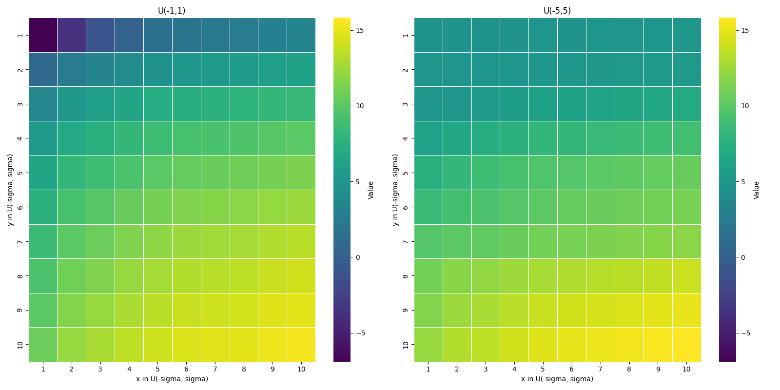
Figure 7: Heatmap showing evolution of log of squared error $\epsilon$ with $D^{t}_{I}=D^{t}_{F}=U(-\sigma,\sigma)$ on polynomials of degree 3 for $\sigma\in\{1,...,10\}$ for the models M135, the left trained on $D_{I}=D_{F}=U(-1,1)$ and the right on $D_{I}=D_{F}=U(-5,5)$.

We define error rate $r_{\epsilon}=\frac{\epsilon_{\sigma}}{|\epsilon_{*}-\epsilon_{0}|}$ where $\epsilon_{*}$ is the best $\epsilon_{\sigma}$ error for a model M with $\hat{f}(x)$ calculated with Least Squares, and $\epsilon_{0}$ is the worst $\epsilon_{\sigma}$ error for a model $M$ such that $\hat{f}_{M}(x)=0$, $\forall x$. In all our error calculations, we exclude the first $n+1$ predictions of each batch from the squared error calculation for $f\in{\cal P}^{n}$, since we need at least n+1 points to be able to find $f$ and the first n+1 predictions by the model are hence almost always wrong. The heatmap in Figure 7 in the Appendix C shows evolution of squared error on two different models.

To ensure that comparisons between models are meaningful, for each $U(-\sigma,\sigma)$, we set a seed when generating the 100 random linear functions, ensuring that each model sees the same randomly chosen functions and the same set of prompting points $x_{i}$. The interest of this test is to see how models perform on tests where they progressively see more out of distribution data (Appendix F).

Training models from scratch on different classes ${\cal P}_{n}$, we found:

Observation 1.

All models ICL₁ functions from ${\cal P}^{n}$ for $n\leq 6$ when $D^{t}_{I}=D_{I}=U(-1,1)$ and $D_{F}=D^{t}_{F}=U(-1,1)$ with a performance in line with optimal algorithms.

Figure 1 shows the generalization ability of our best model on a sampling from $U(-1,1)$ of classes of polynomial functions. We tested up models $Mn$ for $1\leq n\leq 6$. Mn is trained on polynomials in ${\cal P}^{n}$ with coefficients and input values samples from $U(-1,1)$. The models are tested at inference time on functions in ${\cal P}^{n}$ with coefficients sampled from $U(-\sigma,\sigma)$ for $1\leq\sigma\leq 10$.

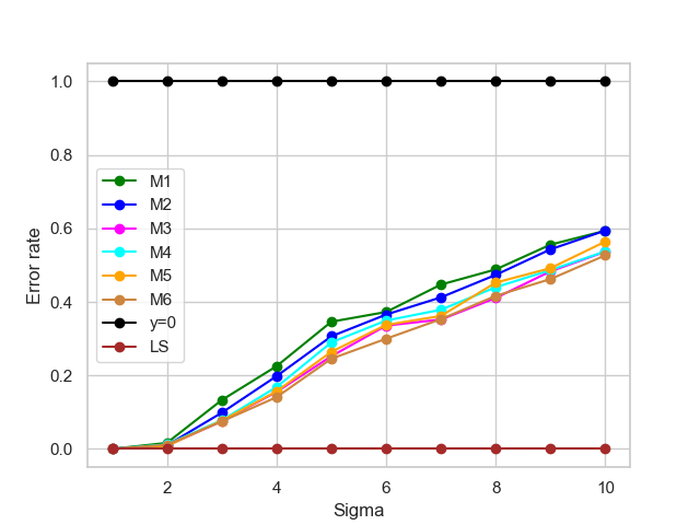
Figure 1: Evolution of error rates for various 12L8AH $d_{emb}=256$ models with $D_{F},D_{I}=D^{t}_{I}=U(-1,1)$ and $D^{t}_{F}$ for various $U(-\sigma,\sigma)$ trained from scratch, each on a different degree. E.g., Mn is a model trained on ${\cal P}^{n}$. The purple curves illustrate a model that predicts $f(x_{n})=0,\forall f$ and $\forall x_{n}$. The dark red line LS represents a perfect estimator given our totally clean input data.

Our experiments showed that all models had the same error rates, and that changing the distribution from Uniform to Gaussian did not change results (see Appendix B). Table 3 shows that some of our models trained on specific polynomial classes ${\cal P}^{n}$ do better as $n$ increases; e.g., models trained only on ${\cal P}^{1}$ do worse on generalizing to functions outside the training distribution than models trained only on ${\cal P}^{2}$, ${\cal P}^{3}$, ${\cal P}^{4}$ or ${\cal P}^{5}$. This runs counter to what one would expect, were the model using least squares or some approximation of it.

Let $f_{/[a,b]}$ denote $\{f(x):x\in[a,b]\}$. Given that we noticed no drop in error rate for more complex polynomials in our models’ predictions, we generalize Observation 1 in two important ways.

Observation 2.

Transformer models ICL₁ $f_{/[a,b]}$ for relatively small $[a,b]$ and $f\in{\cal P}^{n}$ for any $n$ with $D^{t}_{I}=D_{I}$, and $D_{F}=D^{t}_{F}$ with coefficients of $f,x$ sampled from a uniform, normal or even bimodal distribution over $[a,b]$.

models  $\backslash$  $\sigma$	1	2	3	4	5	6	7	8	9	10
$U(-1,1)$	0.0	0.03	0.55	1.37	4.0	5.17	9.04	12.07	19.28	27.85
$U(-5,5)$	0.01	0.01	0.02	0.03	0.03	0.05	0.12	0.27	0.75	1.61
$U(-10,10)$	0.13	0.15	0.17	0.2	0.26	0.26	0.32	0.35	0.41	0.49
$U(-100,100)$	2217.84	2373.82	2494.31	2526.93	2472.45	2467.52	2317.92	2232.03	2129.0	2092.81

Table 1: Comparison showing the evolution of squared errors for models trained on different distributions $D_{I}=D_{F}=U(-a,a)$, for $a=1,5$ or $100$ sampling from ${\cal P}^{1}$ with $D^{t}_{i}=U(-1,1)$ and $D^{t}_{F}=U(-\sigma,\sigma)$.

Observation 2 is significant in virtue of the following:

Theorem 1.

(Stone-Weierstrass) Suppose $f$ is a continuous function defined on $[a,b]\subset\mathbb{H}$, a compact Hausdorf space. $\forall\epsilon>0$ there exists a polynomial function $f_{p}$ such that $\forall x\in[a,b],||f(x)-f_{p}(x)||<\epsilon$

(Brosowski & Deutsch, 1981) provide a generalization of Theorem 1 to any compact space. But for our purposes a closed interval $[a,b]\subset\mathbb{R}$ or is sufficient. The proof uses the approximation of $f$ with Bernstein polynomials, $b_{n}(f)$, which are defined as follows: for $n\in\mathbb{N}_{>0}$, $b_{n}(f):[0,1]\rightarrow\mathbb{R}$ with $x\mapsto\Sigma_{i=0}^{n}f(k/n)\binom{n}{k}x^{k}(1-x)^{n-k}$. To provide the rate of convergence with $b_{n}(f)$ and $\omega_{f}(\alpha)=sup_{|x-y|<\alpha}\{|f(x)-f(y)\}$, we have:

$$|b_{n}(f)(x)-f(x)|=$$

$$|\Sigma_{i=0}^{n}f(k/n)-f(x)\binom{n}{k}x^{k}(1-x)^{n-k}|\leq\frac{3}{2}\omega_{f}(\frac{1}{\sqrt{n}})$$

Note that as $\alpha\rightarrow 0,\omega_{f}(\alpha)\rightarrow 0$ Thus the bounds on convergence are quite strong.

Using Observation 2 and Theorem 1,

Corollary 1.

Transformer models can in principle ICL₁ any continuous, not necessarily differentiable function (see appendix C) $f$ over a small interval $[a,b]$ if we pick a suitable training = testing regime.

We showcase model behavior on three classical continuous functions, exponential, sine, and ln(1+x), with their Taylor series expansions below. After training on ${\cal P}_{3}~$ $D_{F}=D_{I}=N(0,1)$ our models ICL:
$\forall x\in[0,1]$: $e^{x}=\Sigma_{n=0}^{\infty}\frac{x^{n}}{n!}=1+x+\frac{x^{2}}{2}+\frac{x^{3}}{6}+o(||x^{3}||)$
$sin(x)=\Sigma_{n=0}^{\infty}(-1)^{n}\frac{x^{2n+1}}{(2n+1)!}=1-\frac{x^{3}}{6}+o(||x^{3}||)$
$ln(1+x)=\Sigma_{n=1}^{\infty}(-1)^{n+1}\frac{x^{n}}{n}=x-\frac{x^{2}}{2}+\frac{x^{3}}{3}+o(||x^{3}||)$

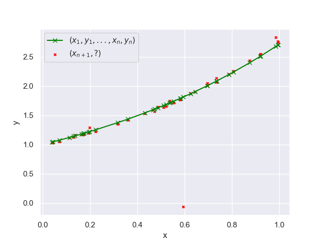
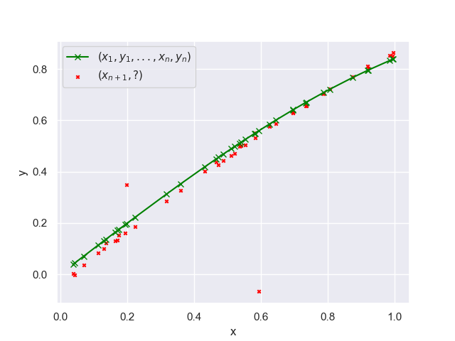
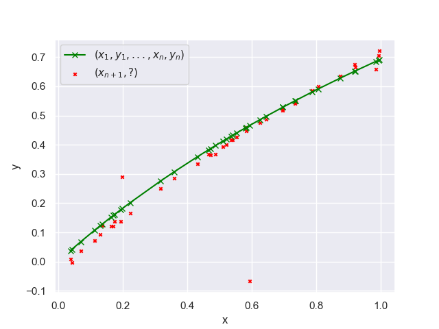
Figure 2: Plot of ICL of $e^{x}$, $sin(x)$ and $ln(1+x)$ by the model trained on ${\cal P}^{3}$.

Once we have fixed the architecture at 12L8AH, increasing $d_{emb}$ from 64 to 512 does not affect performance. We remark that our models are able just from a few prompts like $(x,exp(x))$ or $(x,ln(1+x))$ to differentiate and approximate these functions, even though it has only seen polynomial functions in training.

An interesting observation is that our models did better than an optimal algorithm like LS, because they were able to approximate polynomial functions without knowing their polynomial class. With LS we need to know the equation’s degree.

Our experiments showed several factors affecting the quality of a model’s predictions. First, when $D^{t}_{F}\subset D_{F}$ and $D^{t}_{I}\subset D_{I}$ the model’s performances are substantially increased. Under these conditions, a consistent performance disparity is observed between different models (Table 1 and Heatmap 7). One important criterion we identified by modifying the training distribution and progressively expanding its range is the proportion of points from the test distribution that the model was exposed to during training relative to the total number of points encountered throughout the training process (Table 1). See Appendix H for a mathematical calculation of the proportion for uniform distributions.

One might think that the total number of points observed in the distribution, rather than the proportion, is the critical factor. We tested this alternative hypothesis by training one model on $U(-1,1)$ but for $100k$ steps in one case and another on in $U(-5,5)$ for $500k$ steps, ensuring that both models were exposed to a statistically equivalent number of points within the interval $[-1,1]$. The results remained similar, showing that the total number of points observed is not the critical factor. This was further confirmed through a checkpoint analysis, indicating that optimal performance is typically reached at a fixed training steps. Beyond this point, performance fluctuates, suggesting that exposing the model to a larger number of data points does not necessarily improve performance and may even slightly degrade it.

5 Transformers don’t ICL₂ any $f\in{\cal P}^{n}$

In this section, we show: (i) models do not ICL₂ any functions we tested; (ii) models have similar out of distribution behavior for all functions; (iii) models with attention layers (AL) are needed to achieve ICL and that attention only models can sometimes out perform full transformer architectures

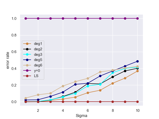
Figure 4: Evolution of error rates for various 12L8AH $d_{emb}=256$ models with $D_{F},D_{I}=D^{t}_{I}=N(0,1)$ and $D^{t}_{F}$ for various $N(0,\sigma)$ trained from scratch on different degrees. The purple curves illustrate a model that predicts $f(x_{n})=0,\forall f$ and $\forall x_{n}$. The dark red line LS represents a perfect estimator given our totally clean input data.

All our models had systematic and non 0 average error on target functions for all polynomial classes tested once we chose either: (i) test distributions over significantly larger intervals than those of training distributions, or (ii) very large training distributions. Figure 1 shows that the error rate increases substantially; Table 3 in the Appendix provides the average errors with respect to least squares and shows that the error rate increases non-linearly as $D_{F}^{t}=U(-\sigma,\sigma)$ and $\sigma$ increase. Figure 7 in Appendix C gives a heatmap rendition of the error across $x_{i}$ and function coefficients. Figure 4 in Appendix B shows similar results for training and testing with $N(0,\sigma)$. Performance did not significantly improve when we moved from models with 9.5 M to 38M parameters.

We found that what (Naim & Asher, 2024b) called boundary values account for this significant increase in error.

Observation 3.

(i) For all models $M$ there exist boundary values $B^{-},B^{+}$ such that for $f(v)\in[B^{-},B^{+}]$, the predictions are close to optimal; (ii) When $f(v)\in[B^{+},B^{+}+\alpha]$, $\hat{f}_{M}(v)\approx B^{-}$, where $\alpha$ is a constant determined by $M$. Similarly, when $f(v)\in[B^{-}-\alpha,B^{-}]$ $\hat{f}_{M}(v)\approx B^{-}$. (ii) When $f(x)>B^{+}+\alpha$ or $<B^{-}-\alpha$, $\hat{f}(v)$ takes random values in $[B^{-},B^{+}]$.

Boundary values occur with all models (For illustrations see Appendix E). To investigate these values, which prevent the model from generalizing, we conducted an ablation study. We first removed the MLP components from our models architecture, but the models continued to exhibit boundary values. We then removed layer normalization; normalization might prevent our models from exceeding certain thresholds, since the output of multi-attention heads and residual learning at layer $i+1$, $Attention(X_{i})+X_{i}$, can theoretically take on large values for example $X=1000X_{i}$. However, even without layer normalization, the phenomenon persisted. Next, we removed residual learning, resulting in a 12-layer model with 8 attention heads only, excluding both ”add and norm” components and MLP. Surprisingly, the boundary values remained, indicating that they originate from the multi-head attention mechanism. Experiments with linear attention only models also exhibit boundary values, so softmax alone does not account for them. In fact for large values softmax functions like hardmax (see Appendix F).

We then tested the learned embedding $\epsilon:\mathbb{R}\rightarrow X^{256}$ to see whether it mapped large values like $Z$ into $[B^{-},B^{+}]$. We mapped with t-SNE $\epsilon[-999,999]$ for our best model and saw that our training induces an almost perfect linear order on values and sufficiently respects mathematical operations so that $Attention(X_{i})+X_{i}$ should provide large values (see Appendix F). The derivation on attention in Appendix F makes the details explicit, and shows that a 1L8AH model, in theory, can not exhibit boundary values, provided linear attention provides a linear operation on $\mathbb{R}$. However, the model experimentally shows boundary values.

This provides a proof outline that:

Proposition 1.

$Attention(X_{i})+X_{i}$ is a non-linear map on $\mathbb{R}$ and on intervals $[a,b]$ that are significantly larger than $[B^{-},B^{+}]$; but can well be linear on the finite field ${\cal F}_{[B^{-},B^{+}]}=([B^{-},B^{+}],+_{\cal F},\times_{\cal F},0_{\cal F},1_{\cal F})$.

Boundary values are intrinsic to the attention mechanism and follow from a model’s pretraining. Attention provide the model a ’shell’ to guard against unrecognized large values. Such a phenomenon becomes problematic in scenarios where the training domain or the underlying mechanism itself is not well understood.

Observation 4.

Our models cannot $ICL_{2}$ functions in ${\cal P}^{n}$, for any $n$.

Were our models able to $ICL$ class forms of polynomials, we would expect much better out of distribution performance; once the parameters for the polynomial form of $f$ are set, f(x) is calculable for all $x$. But we did not observe this; on the contrary we found model performance excellent on arbitrary polynomials over restricted intervals and then bad predictions of the sort described in Observation 3. Also we saw predictions vary over batches in test for the same function, indicating sensitivity to data input, which should not affect parameter estimation for function classes at least for $f\in{\cal P}^{1}$; if $M$ had implemented linear regression, it should get the same result on each batch for $f$.

Observation 4 and Proposition 1 conform to (Asher et al., 2023)’s characterization of learnability. An ICL₂ grasp of any such function class would involve an ability to predict with the same accuracy function values $f(x_{i})$ for $x_{i}$ in arbitrary intervals of $\mathbb{R}$ and for arbitrarily many such points. The same holds for basic arithmetic operations and linear projections on $\mathbb{R}$. (Asher et al., 2023) show that LLMs cannot learn any such sets using ordinary LLM assumptions, and so basic linear operations are linear on finite fields like ${\cal F}_{[B^{-},B^{+}]}$ without being so on $\mathbb{R}$.

In sum, (for discussion and figures see Appendix E, F, H),

Observation 5.

(i) ICL₁ predictions depend on: (i) the presence of attention layers; (ii) the precise values in the prompt (as well as length); (iii) the proportion of the sequences in training in test.

An important consequence of Observations 4 and 5 is that we should not claim that models can ICL any function class unless we specify the interval $[a,b]$ from which their training distributions are sampled. To use ICL with transformer models effectively, we need to know the training regimes of those models. The positive consequence these observations is that judicious choices of pretraining can optimize ICL performance in particular tasks.

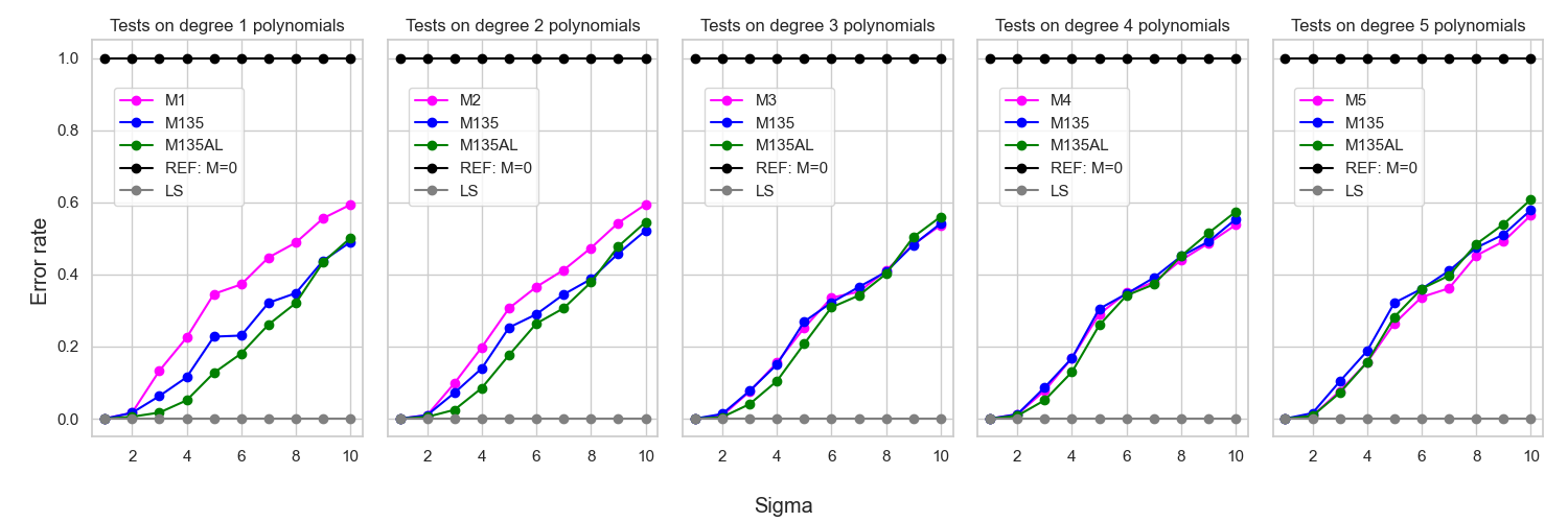
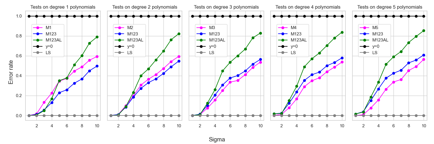
Figure 3: First line of graphs gives error rates for M135, a full 12L8AH transformer model trained on $f\in{\cal P}^{1,2,3}$ (${\cal P}^{1}\cup{\cal P}^{3}\cup{\cal P}^{5}$ with values and inputs sampled from $U(-1,1)$, Mn the same model trained only on $f\in{\cal P}^{n}$ and M135AL, a 12L8AH model with only attention layers and no MLP layers. All models were tested on polynomials of degrees 1-5. Second line gives similar results for models trained on ${\cal P}^{1,2,3}$.

6 Surprising ICL capacities: Generalizing to unseen polynomial classes

We have examined in Sections 4 and 5 models trained and tested on one class of polynomial, with the results in Figure 4. How might a sort of curriculum learning, where models learn several models but not others affect performance? Figure 3 depicts two situations: one in which the models learn to approximate $f\in{\cal P}^{m}$ for $1\leq m\leq 6$ while having been trained on $f\in{\cal P}^{1,2,3}={\cal P}^{1}\cup{\cal P}^{2}\cup{\cal P}^{3}$); the other in which the models train on $f\in{\cal P}^{1,3,5}$. The second case is interesting because it forces the model to predict values for functions of classes on classes it has not seen that lie between classes it has trained on. Figure 3 compares how those models do with respect to models $Mm$ trained and evaluated only on ${\cal P}^{m}$.

While all training regimes produced close to perfect results when test values for coefficients of $f$ and $x\in[-2,2]$, once test values were outside $[-2,2]$, the M1,2 models had much higher error rates than the second “gappy” model M135 on $f\in{\cal P}^{1,2}$. And M135 didn’t even see any quadratic functions in its training. M135 had better generalization performance and error rates better or equal to the best Mm models for any ${\cal P}^{m}$ class we tested. M135 had better results on polynomials of degrees 2 and 4 than it did on $f\in{\cal P}^{5}$. It also had better generalization performance than the cumulative curriculum model M123. M123 also did better than M1 models on ${\cal P}^{1,2}$ but not on higher order polynomial classes. Interestingly, M135AL with attention only layers had optimal or close to optimal performance in many cases, while M123AL had significantly worse generalization performance than other models.

A possible explanation of the superior performance of M123 and M135 over M1 and M2 is this. While higher order polynomial functions define more complex sequences than lower order ones, training on ${\cal P}^{4}$ with coefficients and inputs $x_{i}$ in $U(-1,1)$ will yield a significantly larger spread of values ( in $[-5,5]$) when training on $U(-1,1)$ than training just on ${\cal P}^{1}$. Given our observations that proximity of training is important to accurate approximation, training on higher polynomial classes can aid in generalization. This also accounts for why M123 performs less well than M4 or M5 when we test M123 on ${\cal P}^{4,5}$ and why M135’s superior performance vanishes for higher order polynomials, since training ${\cal P}^{5}$ with sampling from $U(-1,1)$ only negligibly increased the chances of having nearby values from training during inference on, say, ${\cal P}^{3}$ with coefficients sampled from $U(-6,6)$–the maximum values for ${\cal P}^{3}$ on $U(-6,6)$ are included in the interval $[-1514,1514]$, while the maximum training value interval is $[-5,5]$.

In contrast to (Yu et al., 2023), our experiments reveal that the M135AL model demonstrates strong performance and generalizes effectively, even outperforming M135, whereas the M123AL model does not exhibit similar capabilities. These findings suggest that the chosen training methodology significantly influences a model’s propensity to favor reasoning over memorization ceteris paribus.

Observation 6.

A model’s training method can strongly influence performance.

7 Surprising ICL capacities: finding zeros of unknown functions

Since our models treat prompts $(x_{1},f(x_{1}),..,x_{n},?)$ simply as sequences, we can use the same training as in Section 4 to solve a difficult inverse problem: given a prompt of the form $(f(x_{1}),x_{1},..,f(x_{n-1}),x_{n-1},f(x_{n})=0,?)=(y_{1},f^{-1}(y_{1}),...,0,?)$. With this prompt, the $?$ asks M to predict $\hat{x_{n}}=x_{n}+\epsilon$, where $x_{n}$ is the true zero of the function $f$, with $\epsilon$. an error term. For example let $f(x)=x+3$ and so $f^{-1}(x)=x-3$. To find the zero of $f$, we give $f^{-1}(0)=-3$ as then element of our sequence answering to ?.

There are polynomials do not have analytic solutions in terms of radicals, and Galois (Stewart, 2022) gave a necessary and sufficient group theoretic condition for solvability using radicals.

Our models were not trained to provide multiple approximations of multiple roots—i.e., multiple values for ? in $(f^{-1}(x_{1}),x_{1},..,f^{-1}(x_{n}),x_{n},f^{-1}(0),?)$. So we restricted our task to continuous functions that are monotone in addition, as this ensures $f$ is bijective.Thus, $f^{-1}$ is continuous, and Corollary 1 applies.

As an illustrative example of our method, consider the polynomial $f(x)=x^{5}-x+1$. $f(x)=0$, when $x\approx-1.18$. Its plot is in Appendix C. Our best model predicts $\hat{x}=-1.4370$; $f$’s only real root is approximately -1.18. In comparison, an attempt to use Newton’s method to find the $zero$ fails with starting point $x=0$.

One might think that limiting to the case of bijective functions is restrictive, but it’s not much of a restriction. We can reduce the space where we’re looking for the zero so that the function is monotonic there. We tried this on higher-degree polynomials that have several 0’s, and the model did pretty well when we set the search domain where the function is monotone.

We evaluated models using a diverse dataset of over 200 continuous functions. For each function, we provided 64 distinct prompt batches, each of size 40. The model generated a candidate solution for the zero of the function based on the prompts. The prediction was considered correct if at least 70% of the batches satisfied the constraint that the batch prediction for the zero, $x_{M}$, is such that: $||x^{*}-{\hat{x}}_{M}||<\frac{2||x^{*}||}{10},$ where $x^{*}$ is the true zero of $f$, $f(x^{*})=0$. If $x^{*}=0$, we use $0.1$ as upper bound.

The results are in Table 2. Except in 2 or 3 cases, our model’s predicted values could potentially have been accepted if we had loosened our metric. However, for GPT-4, the false values are always far from the correct value. Especially noteworthy is the performance of the M135 AL Attention Layer only model, which had the best overall score.

Models	selected functions	Overall score
M3	87%	52% (104/200)
M135	100%	69.5% (139/200)
M135AL	98%	73.5% (147/200)
GPT4	7%	9 % (18/200)

Table 2: Comparison between our models M3, M135 and M135AL trained from scratch on a sampling of $f\in{\cal P}^{3}$ and gpt4 for finding the zero of an unknown continuous function

These scores are indicative, as they depend on the sample of functions chosen. The class of selected functions included exponential, log, cos, sin and tan, for which the inverses are particularly well behaved (see Table 5 for more details). The models $M135$, $M135AL$ and $M3$ had very high scores. On polynomial functions with inverses that are more complex (and that may induce the problem of several 0), our models had more difficulty, but they were still way better than GPT4 apart from M135AL on ${\cal P}^{1}$ (Appendix G has more details). Nevertheless, our small models show great potential in solving this problem, which suggests smaller LLMs can sometimes replace algorithms like Newton’s Algorithm, which doesn’t necessarily converge and requires both knowing the expression of the function as well as the derivative of the function. Our models do not even require the function to be derivable. Nor do we need particular points with methods like the Dichotomy Principle. If we want greater precision, once we get the the value ${\hat{x}}_{M}$ from the model M, we can take a prompt of type $(f(x_{1}),x_{1},...,f(x_{n}),x_{n},0,?)$ and then verify if $\hat{f}({\hat{x}}_{M})=0$. If it is not, we can still use ${\hat{x}}_{M}$ as a starting point for 0-finding algorithms, like Newton’s algorithm, which depends on an initial point.

8 Discussion

Given our models’ surprising capacities, analysing ICL as a matter largely of associative memory as in (Bietti et al., 2024) needs revisiting. The lack of generalizability from Observations 4 might suggest our models overfit the data and rely solely on memory to ICL. However, the pretraining data has no noise, and it’s too large to be memorized by our models; our largest models with 256 size embeddings have $<10^{7}$ parameters; each parameter would have to encode on average sequences for over 100 different functions of wildly different kinds. Further, some attention-only models in Figure 3 with only 3+ million parameters have equivalent performance to our best models with 10M parameters.

Moreover, our models performed similarly on several different training distributions for $D_{F}$ and $D_{I}$ and tested on $U(-\sigma,\sigma)$ for $\sigma\in\{1,2\}$. Finally, given that 100 samplings with $D^{t}_{F}=U(-2,2)$ nets on average 25 functions with coefficients the model trained on $D_{F}=D_{I}=U(-1,1)$ has not seen (see Appendix Section I), we would expect that if only memory were involved, the model’s error rate on $U(-2,2)$ would be substantially higher than it is. The generalization abilities in Section 6 of our models and their ability to calculate zeros in Section 7 also suggests that ICL involves more than associative memory.

Interestingly, it is the training regime in which the model must predict sequences from function classes it has not seen in training that forces the model to generalize better, as we see from the strong performance of the M135 and M135AL models. This also shows that AL only models can generalize given the right training. Of course, associative memory still plays an important role. Clearly, boundary values are stored and from Observation 3 strongly affect prediction.

Our models’ diverse capacities (but limited in terms of generalization) come from their ability to estimate continuations of a given sequence using principally their attention layers. Given that $Attention(X_{i})+X_{i}$ takes the attention layer output and adds $X_{i}$, we can calculate the limit of seen values when training over uniform distributions. These correspond empirically to the interval given by the model’s boundary values $B^{-},B^{+}$. Thus, given an input $x=(x_{1},...x_{n})$, attention defines a projection $A(x)\mapsto[B^{-},B^{+}]$ Attention layers successively refine this projection to predict $\hat{f}(x_{n})$, as we have seen that multiple layers and multiple heads improve performance.

We have seen that the projection $A$ is effectively nonlinear on elements outside of $[B^{-},B^{+}]$. This limitation is due, we conjecture, to training on a restricted interval. Nevertheless, the limitation is not easily removed. While training with distributions over much larger intervals, for example $U(-100,100)$, might make the attention projection linear over a larger field than ${\cal F}_{[B^{-},B^{+}]}$ (the one defined over $[B^{-},B^{+}]$), Table 1 shows that such training results in very bad performance on all the testing scenarios we tried. Thus, we see a dilemma: training on restricted intervals is needed for good results, but it inevitably hampers generalizability.

9 Conclusion

We have distinguished two notions of learning of mathematical functions: ICL₁, the learning of function graphs over restricted intervals, and ICL₂, the learning of a class form $a_{1}x^{n}+a_{2}x^{n-1}+...a_{n}$ for a function in ${\cal P}^{n}$. We have shown that transformer models can ICL₁ any continuous function within selected intervals. Our pretrained models also acquired surprising learning capacities on unseen polynomial classes and on finding zeros of polynomials, which they did better than state of the art LLMs. However, we have also shown a systematic failure of generalization for decoder-only transformer models of various sizes (up to 9.5 million parameters) and architectures, even when trained on non-noisy data. We have isolated the cause of this problem in the attention mechanism and in its pretraining. Given our results and the discussion above, we do not see an easy solution to this problem.

Impact Statement

The implications of this work are important not only for understanding ICL but also for optimizing its practice. First, ICL has limited generalization abilities with respect to out of training distribution data, but it seems highly capable at least in modeling mathematical functions when training and testing distributions for data are aligned. Second, users of ICL should know the training regime of the models; trying to ICL functions outside the training distribution will very likely lead to degraded results that can importantly affect downstream tasks. So if users are not pretraining the models themselves, then the model builders should make training data and distributions available. Though we are working on very simple data, it is highly likely that this lesson applies to ICL in more challenging areas like NLP.

Appendix A Training details

Additional training information: We use the Adam optimizer (Diederik, 2014) , and a learning rate of $10^{-4}$ for all models.
Computational resources: We used 1 GPU Nvidia Volta (V100 - 7,8 Tflops DP) for every training involved in these experiments.

Appendix B Error rates with Gaussian test and training distributions

When $D_{I}=D_{F}=N(0,\sigma)$ there is for $x\in N(0,\sigma)$ an over 85% chance of $f(x)\in[-4\sigma^{2}-2\sigma,4\sigma^{2}+2\sigma]$ and a 95% chance $f(x)\in[-2\sigma,2\sigma]$. So a model with $\sigma=1$ $D_{F}=D_{I}=N(0,1)$ has seen sequences of values for $f$ with $f(x)\in[-2,2]$ more than 95% of the time.

Appendix C Graphs for $|x|$ and for $f(x)=x^{5}-x+1$

See figures 6 and 5

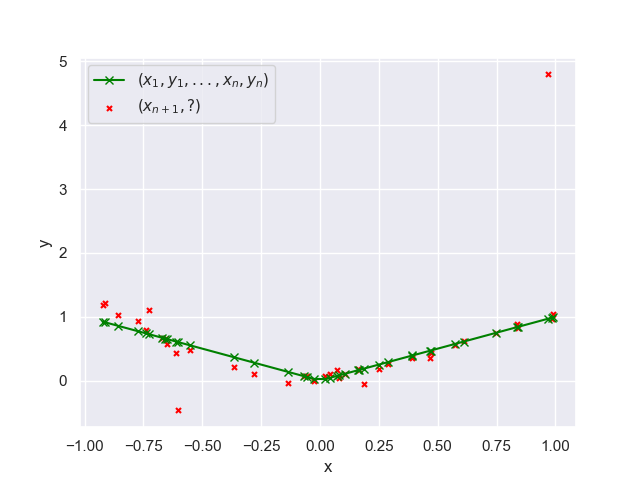
Figure 5: Plots for model $P^{3}$ for the prediction of $f(x)$=$|x|$

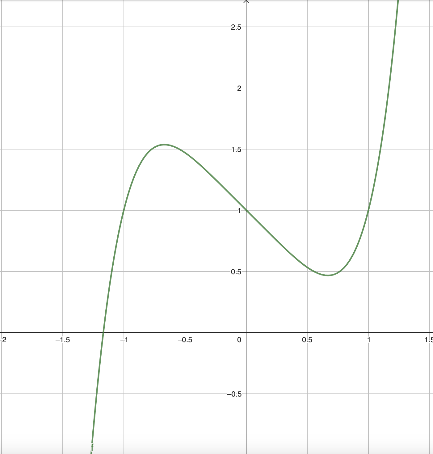
Figure 6: Shape of $f(x)$=$x^{5}-x+1$

Based on Galois’ theorem, this polynomial has only one real value and which can be only determined approximately. When we apply Newton’s method to look for its zero, choosing starting point $x=0$, the method does not converge.

Appendix D Error progression for models trained on $U(-1,1)$ and tested on $U(-\sigma,\sigma)$

degree	models  /  $\sigma$	1	2	3	4	5	6	7	8	9	10
1	M1	0.0	0.03	0.55	1.37	4.0	5.17	9.04	12.07	19.28	27.85
	M135	0.0	0.03	0.26	0.7	2.63	3.2	6.5	8.61	15.21	22.98
	M135AL	0.0	0.01	0.07	0.31	1.47	2.51	5.28	7.93	15.06	23.52
	REF: y=0	0.46	1.84	4.14	6.09	11.56	13.88	20.22	24.72	34.69	46.92
2	M2	0.0	0.02	0.48	1.49	4.01	6.41	9.69	13.11	19.96	32.97
	M135	0.0	0.02	0.35	1.05	3.31	5.08	8.1	10.72	16.84	28.95
	M135AL	0.0	0.01	0.12	0.64	2.31	4.63	7.2	10.47	17.56	30.25
	REF: y=0	0.52	2.05	4.88	7.53	13.09	17.54	23.5	27.69	36.76	55.49
3	M3	0.0	0.02	0.41	1.25	3.69	6.77	9.12	12.14	19.34	31.57
	M135	0.0	0.03	0.42	1.21	3.94	6.5	9.46	12.03	19.3	31.84
	M135AL	0.0	0.01	0.22	0.84	3.04	6.23	8.85	11.87	20.17	32.94
	REF: y=0	0.56	2.27	5.45	8.06	14.64	20.18	25.91	29.56	40.03	58.81
4	M4	0.0	0.03	0.44	1.48	4.66	7.65	10.5	14.47	20.36	32.94
	M135	0.0	0.03	0.49	1.48	4.9	7.59	10.84	14.83	20.55	33.92
	M135AL	0.0	0.02	0.29	1.14	4.17	7.49	10.33	14.84	21.55	35.19
	REF: y=0	0.6	2.45	5.66	8.8	16.08	21.91	27.73	32.9	41.85	61.29
5	M5	0.0	0.02	0.46	1.51	4.52	7.9	10.52	16.4	21.84	37.66
	M135	0.0	0.04	0.62	1.81	5.5	8.43	11.93	17.19	22.69	38.66
	M135AL	0.0	0.02	0.43	1.51	4.83	8.44	11.54	17.56	23.97	40.58
	REF: y=0	0.64	2.57	6.0	9.65	17.11	23.42	29.09	36.25	44.41	66.77

Table 3: Comparison to show the evolution of squared error $\epsilon$, with $D_{i}^{t}=U(-1,1)$, $D_{F}^{t}=U(-\sigma,\sigma)$ for models $M1$, $M135$ and $M135AL$

Appendix E Boundary values

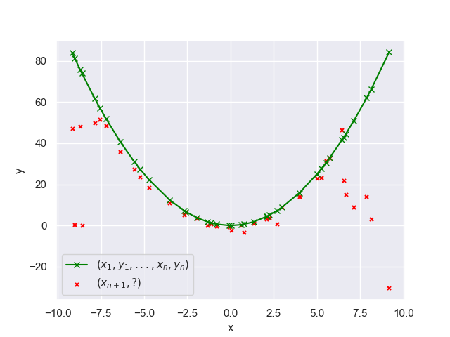
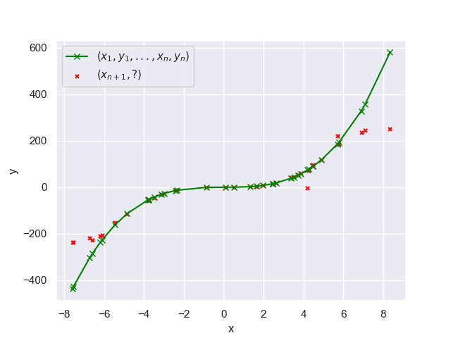
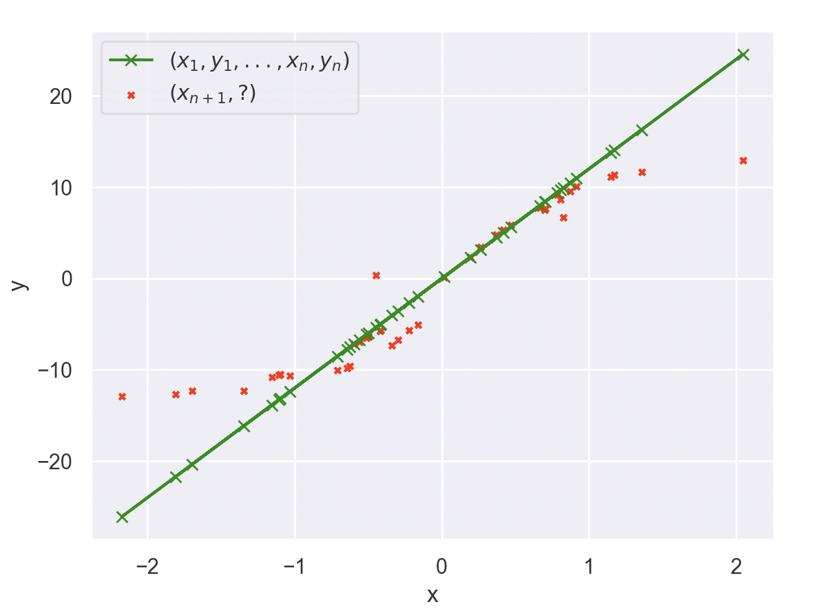
Figure 8: First two plots for models $P2$ for $f(x)=x^{2}$ $P3$ for $f(x)=x^{3}$, trained on $D_{I}=D_{F}=N(0,1)$ showing boundary values. Third plot shows boundary values for 2L32ah attention only model, with $d_{embedding}=256$ to ICL the function $f(x)=12x$.

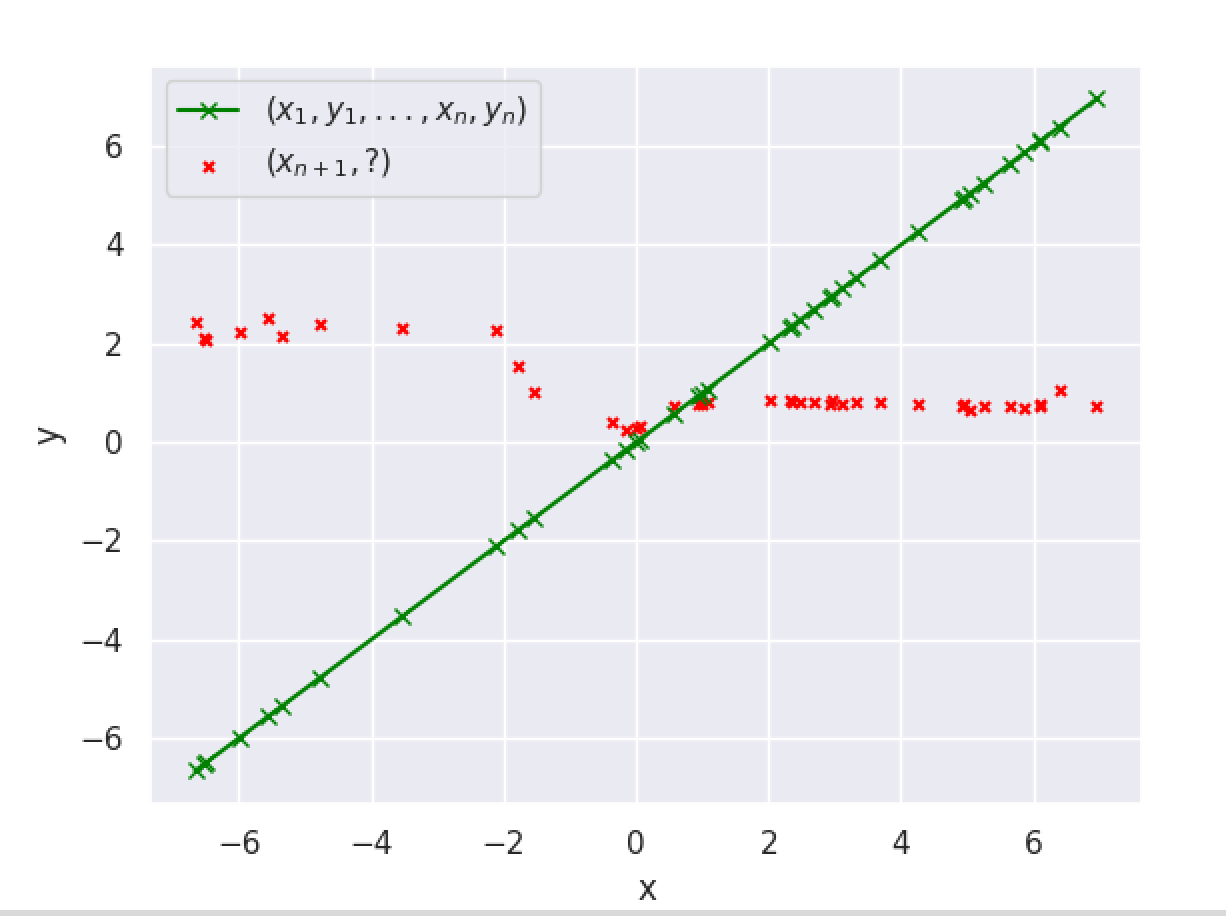
Figure 9: Plot is for $f(x)=x$ on attention only and no norm still showing boundary values.

Appendix F Calculation of what causes boundary values

Given that our ablation study showed the existence of boundary values for models just with attention layers and without residual learning, norm or feed forward linear layers, we analyze the attention mechanism mathematically to see where boundary values could arise/ Let’s consider $X^{l}=(X_{1}^{l},...,X_{n}^{l})$ is the input that goes through the multihead attention in a layer $l$. The output of Multihead Attention after going through 8 attention heads, then a Linear layer is : $(C_{1}^{l},C_{2}^{l},...,C_{n}^{l})$ where

$$C_{i}^{l}=\Sigma^{8}_{h=1}\Sigma^{n}_{k=1}W_{O}^{l}softmax(\frac{(W_{Q}^{h,l}X_{i}^{l})^{T}(W_{K}^{h,l}X_{i}^{l})}{\sqrt{d_{k}}})(W^{h,l}_{V}X_{k}^{l})$$

where $W_{Q}^{h,l},W_{K}^{h,l},W_{V}^{h,l}$ are respectively Query, Key and Value weights matrices in attention head $h$ in layer $l$, $d_{k}$ is the dimension of the key matrix and $W_{O}^{l}$ is the matrix of the linear layer that comes after the attention heads in the layer l. All those matrices have fixed values from training.
To investigate what is causing boundary values into the attention block, Let’s consider a model of 1 layer, and take a fixed $X^{1}=(X_{1}^{1},...,X_{n}^{1})$, we consider also $1000X^{1}=(1000X_{1}^{1},...,1000X_{n}^{1})$.
The output of the model for $1000X^{l}$ is: $(C_{1}^{1},C_{2}^{1},...,C_{n}^{1})$ where

$$C_{i}^{1}=\Sigma^{8}_{h=1}\Sigma^{n}_{i,j=1}W_{O}^{l}softmax(\frac{(W_{Q}^{h,l}1000X_{i}^{l})^{T}(W_{K}^{h,l}1000X_{j}^{l})}{\sqrt{d_{k}}})(W^{h,l}_{V}1000X_{k}^{l})$$ (1)

Now assuming that the learned embedding $\epsilon:\mathbb{R}\rightarrow Z^{256}$, for some set $Z$, somewhat respects arithmetic operations, then $\epsilon(1000X)=\epsilon(a)\times\epsilon(X)$ and we could infer from Equation 1 and the fact that the matrices are all linear projections on $\mathbb{R}$,

$$a\Sigma^{8}_{h=1}\Sigma^{n}_{i,j=1}W_{O}^{l}softmax(10^{6}\frac{(W_{Q}^{h,l}X_{i}^{l})^{T}(W_{K}^{h,l}X_{j}^{l})}{\sqrt{d_{k}}})(W^{h,l}_{V}X_{k}^{l})$$ (2)

The output of each layer will reduce these large values given small values of soft- or even hardmax. But as is evident from Table 4, for large values v, hardmax(v) and softmax(v) give us probability 1 on the greatest value and 0 for the rest. So this derivation predicts that the attention mechanism should give large values for large inputs. But it does not.

This proof rests on two assumptions: (i) the learned embedding somewhat preserves arithmetical operations (ii) the matrices that defined Attention are in fact linear projections in $\mathbb{R}$. We checked the “vanilla” encodings $\epsilon_{V}$ on GPT2, and we saw that that embedding $\epsilon_{V}(a*b)$ is typically not even close using cosine similarity to $\epsilon_{V}(a)*\epsilon_{V}(b)$, where $*$ is some arithmetical operation. However as can be seen from Figure 11, the learned embedding from our pretraining preserves general mathematical operations and induces an almost perfect linear ordering on $[-1000,1000]$. This entails then that at least one of the matrices used to define Attention $W_{Q}^{h,l},W_{K}^{h,l},W_{V}^{h,l}$ is only linear on the small finite field ${\cal F}=([B^{-},B^{+}],+_{\cal F},\times_{\cal F},0_{\cal F},1_{\cal F})$.

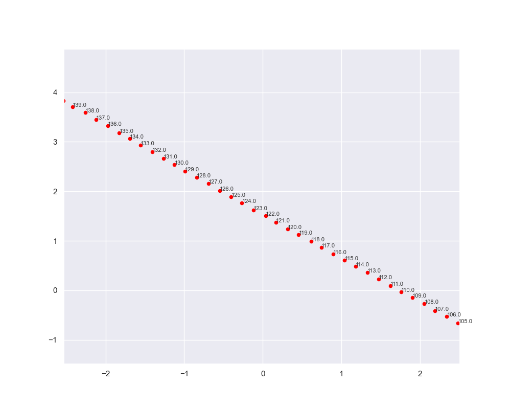
Figure 10: Plot illustrating how embeddings exhibit increasing amplitudes as the values of the real numbers grow, visualized using t-SNE with two dimensions (TSNE-2).

Vector values	Softmax	Vector values	Softmax	Vector values	Softmax
$1$	0.192046	$100$	0.000045	$1$	0
$1.02$	0.195925	$102$	0.000333	$1020$	0
$1.03$	0.197894	$103$	0.000905	$1030$	0
$1.05$	0.201892	$105$	0.006684	$1050$	0
$1.1$	0.212243	$110$	0.992033	$1100$	1

Table 4: Table showing that for large values, softmax performs like hardmax

Appendix G Selected functions for ”finding zeros of unknown functions”

The functions we looked for their zeros with their following scores for different models are for our scores are: $cos(ax)$ for $x\in[0,\pi]$, $a\in[-1,1]$, $sin(ax)$ for $x\in[-\pi/2,\pi/2]$, $a\in[-1,1]$, $tan(ax)$ for $x\in]-\pi/2,\pi/2[$, $a\in[-1,1]$, $aexp(x)-b$ for $a,b\in[0,1],x\in[-1,1]$ and $ln(ax)$ for $a,x\in]0,1]$.

Appendix H More details on Zeros of functions

Table 5

Functions  Models	M3	M135	M135AL	GPT4
$ln$	20/20	20/20	20/20	3/20
$cos$	20/20	20/20	20/20	0/20
$sin$	20/20	20/20	20/20	0/20
$tan$	12/20	20/20	20/20	4/20
$exp$	15/20	20/20	18/20	0/20
$ax+b$	9/20	12/20	0/20	5/20
$(x^{2}+1)(x-a)$	11/20	14/20	17/20	5/20
$(x^{2}+d)((x+2)(x-a)$	7/20	11/20	11/20	0/20

Table 5: Comparison between our models M3, M135 and M135AL trained from scratch on a sampling of $f\in{\cal P}^{3}$ and gpt4 for finding the 0 of an unknown continuous function

Appendix I Calculating proportionality of test in train

Using tests for coefficients on $U(-\sigma,\sigma)$ show us how error rates evolves when we increase the proportion of test elements outside the training distribution. We start by testing on $x$ and coefficients in $U(-1,1)$ where the model have seen all the values, then we go through $U(-1,1)$ where the model has seen fewer values. For example for degree 1, the model has seen values during training $a,b,x\in[-1,1]$ , which means $ax+b\in[-2,2]$

Given $a\in U(-2,2)$ and $x\in U(-1,1)$, $ax\in Z$ where $Z=X_{1}X_{2}$ is the product of two random variables and an addition.
The probability that the model was asked to ICL a value it didn’t see during training is

$$P(X=ax+b\notin[-2,2])=1-P(X=ax+b\in[-2,2])$$

To calculate it, we need first the density of $Z=X_{1}X_{2}$ which is a product of two random variables:
since $X_{1}=X_{3}$ are $U(-2,2)$, then $f_{X_{1}}(x)=f_{X_{3}}(x)=1/4$ if $x\in[-2,2]$ and $0$ otherwise. And $X_{2}$ is $U(-1,1)$ $f_{X_{2}}(x)=1/2$ if $x\in[-1,1]$ and $0$ otherwise.

$f(z)=\int_{-\infty}^{+\infty}f_{X_{1}}(x)f_{X_{2}}(\frac{z}{x})\frac{1}{|x|}dx=\int_{-2}^{2}\frac{1}{4}f_{X_{2}}(\frac{z}{x})\frac{1}{|x|}dx$

$f_{X_{2}}(\frac{z}{x})\neq 0$ when $-1\leq\frac{z}{x}\leq 1$ which means that $\frac{|z|}{|x|}\leq 1$, then $|z|\leq|x|$, so $z\leq x$ or $x\leq-z$, otherwise $f_{X_{2}}(\frac{z}{x})=0$, so $f(z)=\int_{z}^{2}\frac{1}{4}f_{X_{2}}(\frac{z}{x})\frac{1}{|x|}dx+\int_{-2}^{-z}\frac{1}{4}f_{X_{2}}(\frac{z}{x})\frac{1}{|x|}dx=\frac{1}{4}(\frac{1}{2}\int_{z}^{2}\frac{1}{|x|}dx+\frac{1}{2}\int_{-2}^{-z}\frac{1}{|x|}dx)=\frac{1}{4}(\int_{|z|}^{2}\frac{1}{|x|}dx)=\frac{1}{4}ln(\frac{2}{|z|})$
Now that the density of product of two random uniform variables $U(-1,1)$ and $U(-2,2)$ is known, the density of probability of the addition with $U(-1,1)$ $X_{1}X_{2}+X_{3}=Z+X_{3}$ is:

$f(s)=\int_{-\infty}^{+\infty}f_{X_{1}X_{2}}(s-x)f_{X_{3}}(x)dx=\int_{-2}^{2}ln(\frac{2}{|s-x|})\frac{1}{4}dx=\frac{1}{4}\int_{-2}^{2}ln(\frac{2}{|s-x|})dx=\frac{1}{4}\int_{-2}^{2}ln(2)-ln(|s-x|)dx=ln(2)-\frac{1}{4}\int_{-2}^{2}ln(|s-x|)dx$ when $s\in[-4,4]$ otherwise $0$.

The following graph illustrates the situation.

Figure 11: Plot of the density of probability of $X_{1}X_{2}+X_{3}$

Then the out of distribution probability is:

$$P(X=ax+b\notin[-2,2])=1-P(X=ax+b\in[-2,2]),$$

or near $20\%$. Thus we increase gradually the proportion of values not seen during training, each time we increase the value of $\sigma$.

Appendix J Data on prompt length

While at least n+1 points are needed to find a polynomial in ${\cal P}^{n}$ function, all model performance regardless of training distribution degrades when the size of the prompt during inference is greater than the maximal size of prompts seen in training. Figure 12 (Appendix J).

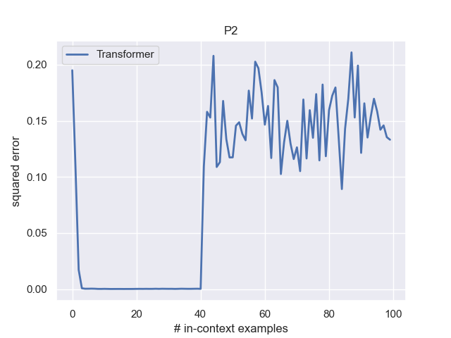
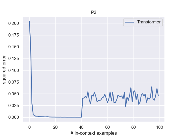
Figure 12: Plot of ICL for $f(x)=x^{2}$ for P2 and $f(x)=x^{3}$ for P3 when increasing retrogressively the size of the prompts to depass the training maximum sequence length.

References

- Akyürek et al. (2022) Akyürek, E., Schuurmans, D., Andreas, J., Ma, T., and Zhou, D. What learning algorithm is in-context learning? investigations with linear models. arXiv preprint arXiv:2211.15661, 2022.
- Asher et al. (2023) Asher, N., Bhar, S., Chaturvedi, A., Hunter, J., and Paul, S. Limits for learning with large language models. In 12th Joint Conference on Lexical and Computational Semantics (*Sem). Association for Computational Linguistics, 2023.
- Bhattamishra et al. (2023) Bhattamishra, S., Patel, A., Blunsom, P., and Kanade, V. Understanding in-context learning in transformers and llms by learning to learn discrete functions. arXiv preprint arXiv:2310.03016, 2023.
- Bietti et al. (2024) Bietti, A., Cabannes, V., Bouchacourt, D., Jegou, H., and Bottou, L. Birth of a transformer: A memory viewpoint. Advances in Neural Information Processing Systems, 36, 2024.