Efficient Image Restoration via Latent Consistency Flow Matching

Abstract

Recent advances in generative image restoration (IR) have demonstrated impressive results. However, these methods are hindered by their substantial size and computational demands, rendering them unsuitable for deployment on edge devices. This work introduces ELIR, an Efficient Latent Image Restoration method. ELIR operates in latent space by first predicting the latent representation of the minimum mean square error (MMSE) estimator and then transporting this estimate to high-quality images using a latent consistency flow-based model. Consequently, ELIR is more than 4x faster compared to the state-of-the-art diffusion and flow-based approaches. Moreover, ELIR is also more than 4x smaller, making it well-suited for deployment on resource-constrained edge devices. Comprehensive evaluations of various image restoration tasks show that ELIR achieves competitive results, effectively balancing distortion and perceptual quality metrics while offering improved efficiency in terms of memory and computation.

{elad.cohen02,idan.achituve,idit.diamant,arnon.netzer,hai.habi}@sony.com

1 Introduction

Image restoration (IR) is a challenging low-level computer vision task focused on generating visually appealing high-quality (HQ) images from low-quality (LQ) images (e.g. noisy, blurry). Image deblurring (Kupyn et al., 2019; Whang et al., 2022), blind face restoration (Wang et al., 2021b; Li et al., 2020), image super-resolution (Dong et al., 2012, 2015), image denoising, inpainting, and colorization can be categorized under IR. The scope of IR applications is extensive, encompassing mobile photography, surveillance, remote sensing, and medical imaging.

Algorithms that tackle the IR problem are commonly evaluated by two types of metrics: 1) a distortion metric (e.g. PSNR) that quantifies some type of discrepancy between the reconstructed images and the ground truth; 2) perceptual quality (PQ) metric (e.g. FID (Heusel et al., 2017)) that intends to assess the appeal of reconstructed images to a human observer. The distortion and PQ metrics are usually at odds with each other leading to a distortion-perception trade-off (Blau & Michaeli, 2018). This trade-off can be viewed as a Pareto frontier, which can be framed as an optimization problem by minimizing distortion while achieving a given perception index. Out of all points on the distortion-perception Pareto frontier, the main goal of the IR task is to find the point where the estimator achieves minimal average distortion under a constraint of perfect perceptual index (Ohayon et al., 2024). A solution for this problem (Freirich et al., 2021) can be obtained by initially using a minimum mean square error (MMSE) estimator, followed by sampling from the posterior distribution of visually appealing images given the MMSE output.

Figure 1: Comparison between ELIR and diffusion & flow-based baselines methods. ELIR is the smallest and fastest method while maintaining PSNR (higher is better) and FID (lower is better) competitive with state-of-the-art results. The results were obtained using the CelebA-Test dataset for blind face restoration.

Recently, several approaches have explored this direction, proposing two-stage algorithms (Yue & Loy, 2024; Lin et al., 2023; Rombach et al., 2022; Zhu et al., 2024; Yue et al., 2024; Ohayon et al., 2024). In the first stage, a neural network is utilized to correct the distortion error. Then, in the second stage, a conditional generative model is employed to sample visually appealing images conditioned on the output of the first stage. Typically, the first stage is trained to minimize a distortion metric (e.g. $\ell_{1}$, $\ell_{2}$), while the second stage is trained using a diffusion (Sohl-Dickstein et al., 2015; Ho et al., 2020) or a flow matching objective. (Albergo & Vanden-Eijnden, 2023; Lipman et al., 2023; Liu et al., 2023)

Although these methods achieve state-of-the-art results, deploying them on edge devices such as mobile phones or image sensors is challenging due to significant memory and computational requirements. The high demands stem from three main reasons: (i) the transformer-based architecture used by these methods, which incurs substantial computation and memory costs; (ii) state-of-the-art approaches based on diffusion or flow matching necessitate multiple neural function evaluations (NFE) during inference, posing difficulties for edge devices; (iii) many methods operate directly in pixel space, demanding high computational costs, particularly at high resolutions.

In this work, we address the challenge of providing an efficient algorithm for IR that exhibits significantly improved resource efficiency in terms of memory consumption and computational cost, while maintaining an equivalent level of performance. We achieve this by suggesting ELIR, an Efficient Latent Image Restoration method. ELIR includes two stages. First, we introduce the Latent MMSE estimator, which computes the conditional expectation of the latent representation given the latent representation of the degraded image, yielding the latent posterior mean. Second, we suggest latent consistency flow matching (LCFM), an integration of latent flow matching (Dao et al., 2023) and consistency flow matching (Yang et al., 2024). To the best of our knowledge, this approach is presented here for the first time. LCFM aims to reduce both the number of NFEs and the computational cost of each NFE. We emphasize that ELIR uniquely integrates Latent MMSE and LCFM, allowing the complete execution of the procedure within the latent space, which significantly reduces the computational costs associated with processing high-resolution images. In addition, we suggest replacing the transformer-based architecture with a convolution-based one that can be efficiently implemented on edge devices.

We conducted a set of experiments to validate ELIR and highlight its benefits in terms of distortion, perceptual quality, model size, and latency. Specifically, we evaluate ELIR on blind face restoration, super-resolution, image denoising, inpainting, and colorization. In all tasks, we demonstrate significant efficiency improvements compared to diffusion & flow-based methods. Our model size is reduced by 4 to 45 times, and we achieve between 4 to 270 times increase in frames per second (FPS) processing speed. ELIR achieves these improvements without sacrificing distortion or perceptual quality, remaining competitive with state-of-the-art approaches (Figure 1).

Our contributions are summarized as follows:

• We introduce the Latent Minimum Mean Square Error estimator (Latent MMSE) which approximates the posterior mean in the latent space.

• We integrate latent flow matching with consistency flow matching for the first time, which reduces the NFEs as well as the cost of each evaluation.

• We performed experiments on various tasks including blind face restoration, image super-resolution, image denoising, inpainting, and colorization. The results show a 4-45$\times$ reduction in memory size and a 4-270$\times$ reduction in latency compared to state-of-the-art diffusion & flow-based methods while maintaining competitive performance.

2 Related Work

Various approaches have been suggested for image restoration (Zhang et al., 2018a, 2021; Luo et al., 2020; Liang et al., 2021; Zhou et al., 2022; Lin et al., 2023; Yue & Loy, 2024; Zhu et al., 2024; Ohayon et al., 2024). In recent years, solutions for IR based on generative methods, including GANs (Goodfellow et al., 2014), diffusion models (Song et al., 2021) and flow matching (Lipman et al., 2023), have emerged, yielding impressive results.

GAN-based methods. GAN-based techniques have been proposed to address image restoration. BSRGAN (Zhang et al., 2021) and Real-ESRGAN (Wang et al., ) are GAN-based methods that use effective degradation modeling process for blind super-resolution. GFPGAN (Wang et al., 2021a) and GPEN (Yang et al., 2021) proposed to leverage GAN priors for blind face restoration. GPEN suggested training a GAN network for high-quality face generation and then embedding it to a network as a decoder before blind face restoration. GFPGAN connected a degradation removal module and a pre-trained face GAN by direct latent code mapping. CodeFormer (Zhou et al., 2022) also uses GAN priors by learning a discrete codebook before using a vector-quantized autoencoder. Similarly, VQFR (Gu et al., 2022) uses a combination of vector quantization and parallel decoding, enabling efficient and effective restoration.

Diffusion-based methods. DDRM (Kawar et al., 2022), DDNM (Wang et al., 2023), and GDP (Fei et al., 2023) are diffusion-based methods that have superior generative capabilities compared to GAN-based methods by incorporating the powerful diffusion model as an additional prior. Under the assumption of known degradations, these methods can effectively restore images in a zero-shot manner. ResShift (Yue et al., 2024) proposed an efficient diffusion model that facilitates the transitions between HQ and LQ images by shifting their residuals. Recently, several approaches have suggested two-stage pipeline algorithms. DifFace (Yue & Loy, 2024) suggested such a method for blind face restoration, performing sampling from a transition distribution followed by a diffusion process. DiffBIR (Lin et al., 2023) proposed to solve blind image restoration by first applying a restoration module for degradation removal and then generating the lost content using a latent diffusion model.

Flow-based methods. Recently, FlowIE (Zhu et al., 2024) and PMRF (Ohayon et al., 2024) introduced two-stage algorithms for image restoration based on rectified flows (Liu et al., 2023). FlowIE relies on the computationally intensive Stable Diffusion (Rombach et al., 2022), which limits its suitability for deployment on edge devices. PMRF has shown impressive results on both perception and distortion metrics by minimizing the MSE under a perfect perceptual index constraint. It alleviates the issues of solving the ODE by adding Gaussian noise to the posterior mean predictions. Nevertheless, PMRF uses sophisticated attention patterns that pose significant challenges for efficient execution on resource-constrained edge devices because of intensive shape and indexing operations (Li et al., 2023). Our work introduces an efficient flow-based method designed with a hardware-friendly architecture, enabling its deployment on resource-constrained edge devices.

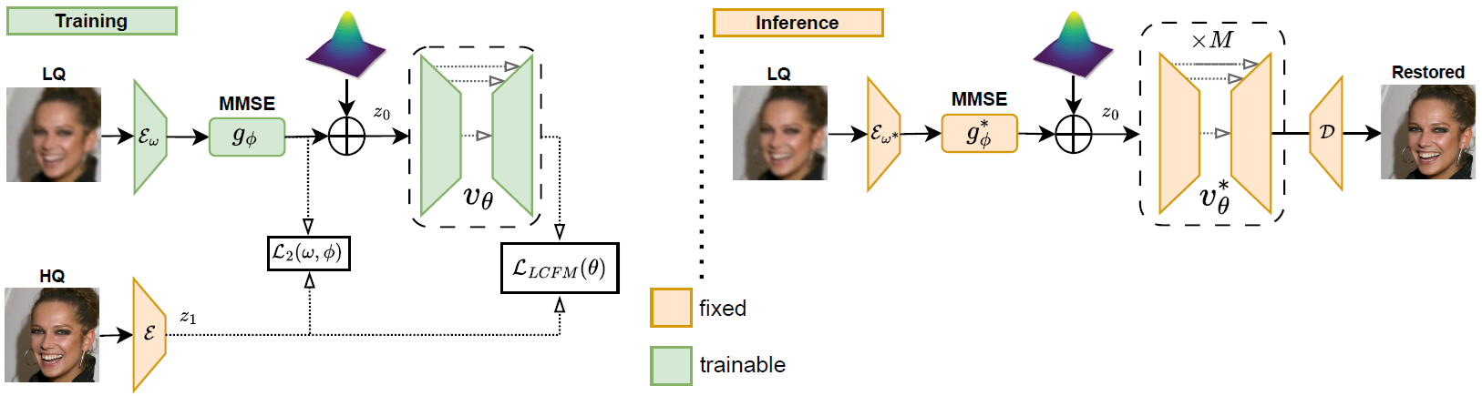
Figure 2: ELIR Overview. During training, we optimize the encoder, MMSE estimator, and the vector field for a specific IR task, to establish direct paths from LQ to HQ image distribution. During inference, we utilize the MMSE estimator and predict a consistent linear direction from LQ toward the HQ images, yielding high-quality results, and balancing distortion and perception. Both training and inference are conducted in latent space.

3 Preliminaries

3.1 Distortion and Perception

The perception of image quality is a complex interplay between objective metrics and subjective human judgment. While objective measures like PSNR and SSIM are useful for quantifying distortion, they may not always correlate well with perceived image quality (Wang et al., 2004). Human observers are sensitive to artifacts and inconsistencies, even when they are subtle. Effective image restoration techniques must therefore aim to minimize both objective distortion and perceptual artifacts, ensuring that the restored image is both visually pleasing and faithful to the original content. Let’s denote the high-quality and the corresponding low-quality images as $\bm{x}$ and $\bm{y}$, respectively, and the reconstructed image by $\bm{\hat{x}}$. The distortion is usually evaluated by $D=\mathbb{E}_{p_{\bm{x},\bm{\hat{x}}}}\left[\Delta\left(\bm{x,\bm{\hat{x}}}\right)\right]$, where $\Delta\left(\bm{x},\bm{\hat{x}}\right)$ is a distance function and $p_{\bm{x},\bm{\hat{x}}}$ is the joint probability function of $\bm{x}$ and $\bm{\hat{x}}$. The distortion-perception trade-off (Blau & Michaeli, 2018) is defined by:

$$D(P)=\mathbb{E}_{p_{\bm{\hat{x}}|\bm{y}}}\left[\Delta\left(\bm{x,\bm{\hat{x}}}\right)\right]\quad s.t\quad d(p_{\hat{\bm{x}}},p_{\bm{x}})\leq P,$$ (1)

where $P$ is some constant, and $d(\cdot)$ is some divergence between probability measures. The goal is to find an estimator that achieves minimal average distortion under a perfect perceptual quality constraint ($P=0$). By setting the $\Delta$ function as the squared distance function, the trade-off can be formalized as:

$$\min_{p_{\hat{\bm{x}}|\bm{y}}}\mathbb{E}\left[\left\lVert\bm{x}-\hat{\bm{x}}\right\rVert_{2}^{2}\right]\quad s.t\quad p_{\hat{\bm{x}}}=p_{\bm{x}}.$$ (2)

Freirich et al. (2021) proved that the optimal solution for Problem 2 is first to obtain the minimum mean square error (MMSE) estimator, $\bm{x}^{*}=\mathbb{E}\left[\bm{x}|\bm{y}\right]$, and then sample from the optimal transport from $p_{\bm{x}^{*}}$ to $p_{\bm{x}}$.

3.2 Consistency Flow Matching

Consistency Flow Matching (CFM) advances flow-based generative models (Chen et al., 2018; Lipman et al., 2023; Liu et al., 2023) by enforcing consistency among learned transformations. This constraint ensures that the transformations produce similar results regardless of the starting point. By utilizing “straight flows” for simplified transformations and employing a multi-segment training strategy, CFM achieves enhanced sample quality and inference efficiency. Specifically, given $\bm{x}$ as an observation in the data space $\mathbb{R}^{d}$, sampled from unknown data distribution, CFM first defines a vector field $\bm{v}(\bm{x}_{t},t):\mathbb{R}^{d}\times[0,1]\xrightarrow{}\mathbb{R}^{d}$, that generates the trajectory $\bm{x}_{t}\in\mathbb{R}^{d}$ through an ordinary differential equation (ODE):

$$\frac{d\bm{x}_{t}}{dt}=\bm{v}(\bm{x}_{t},t).$$ (3)

Yang et al. (2024) suggests to train the vector field by a velocity consistency loss defined as:

$$\mathcal{L}_{CFM}\left(\bm{\theta}\right)=$$ (4)

$$\mathbb{E}_{t}\mathbb{E}_{\bm{x}_{t},\bm{x}_{t+\Delta t}}\left[\Delta f_{\bm{\theta}}\left(\bm{x}_{t},\bm{x}_{t+\Delta t},t\right)+\alpha\Delta v_{\bm{\theta}}\left(\bm{x}_{t},\bm{x}_{t+\Delta t},t\right)\right]$$

where,

$$\Delta v_{\bm{\theta}}\left(\bm{x}_{t},\bm{x}_{t+\Delta t},t\right)=\left\lVert\bm{v}_{\bm{\theta}}(\bm{x}_{t},t)-\bm{v}_{\bm{\theta}^{-}}(\bm{x}_{t+\Delta t},t+\Delta t)\right\rVert_{2}^{2},$$

$$\Delta{f}_{\bm{\theta}}\left(\bm{x}_{t},\bm{x}_{t+\Delta t},t\right)=\left\lVert f_{\bm{\theta}}(\bm{x}_{t},t)-f_{\bm{\theta}^{-}}(\bm{x}_{t+\Delta t},t+\Delta t)\right\rVert_{2}^{2},$$

$$f_{\bm{\theta}}(\bm{x}_{t},t)=\bm{x}_{t}+\left(1-t\right)\bm{v}_{\bm{\theta}}(\bm{x}_{t},t),$$

$t\sim\mathbb{U}[0,1-\Delta t]$ is the uniform distribution, $\Delta t$ is a small time interval and $\alpha$ is a positive scalar. $\bm{\theta}^{-}$ denotes the running average of past values of $\bm{\theta}$ using exponential moving average (EMA).

To apply (4), we require to select a trajectory $\bm{x}_{t}$. Several options exist in the literature (Ho et al., 2020; Lipman et al., 2023; Liu et al., 2023). In this work, we use the optimal-transport conditional flow matching as proposed by Lipman et al. (2023), which enhances both the sampling speed and training stability. This trajectory is defined as

$$\bm{x}_{t}=t\bm{x}_{1}+(1-(1-\sigma_{min})t)\bm{x}_{0},$$ (5)

where $\bm{x}_{0}$ and $\bm{x}_{1}$ are sampled from source and target distribution, respectively, and $\sigma_{min}$ is a hyperparameter.

In inference, solving the ODE with the forward Euler method can produce high-quality results with significantly fewer steps (NFEs) than traditional Flow Matching (FM) techniques.

4 Method

In this work, we address the challenge of developing an efficient method that minimizes average distortion under a perfect perceptual quality constraint as given in (2). By “efficient”, we refer to the model’s memory usage and latency. Specifically, we are given a dataset $\mathcal{S}\triangleq\set{\bm{y}_{i},\bm{x}_{i}}$, consisting of pairs of images where $\bm{y}_{i}$ represents the low-quality (LQ) images and $\bm{x}_{i}$ represents the high-quality (HQ) images. Our objective is to develop a neural network that can solve Problem (2) efficiently. To achieve this, we propose a method based on the problem solution suggested in Freirich et al. (2021), which minimizes the average distortion while maintaining a perfect perceptual quality ($P=0$).

Inspired by this solution, we suggest a two-stage pipeline that operates in latent space. First, we apply a latent MMSE estimator on the LQ input image which reduces the distortion error in the latent space. Second, we utilize a latent consistency flow model which samples from the conditional posterior distribution of latent representation of $\bm{x}$ given results of the latent MMSE Estimator. The entire process is performed in latent space, which enables efficient inference and significantly reduces the computational costs associated with processing high-resolution images. Moreover, we suggest a hardware-friendly architecture consisting of only convolutional layers (see Appendix 7.1). This architecture is highly optimized for most hardware accelerators, leading to reduced model size and latency, making it suitable for resource-constrained edge devices.

An overview of the suggested flow is presented in Figure 2. The latent MMSE and the consistency flow are explained in Subsections  4.1 and 4.2, respectively, and the training and inference procedures are described in Subsection 4.3.

4.1 Latent MMSE

Here, we describe the latent MMSE estimator, which takes the latent representation of the LQ image and restores it to closely match the latent representation of the HQ image in terms of $\ell_{2}$. Specifically, let $\bm{x}$ and $\bm{y}$ be a pair of HQ and LQ images, respectively, $\mathcal{E}_{\bm{\omega}}$ be a pre-trained encoder (parameterized by $\bm{\omega}$) that projects an image to the latent space, and $g_{{\phi}}$ be the latent MMSE estimator (parameterized by $\bm{\phi}$). The objective is to minimize the $\ell_{2}$ difference between the latent representations of the LQ and HQ images, which is given by:

$$\mathcal{L}_{2}\left(\bm{\phi},\bm{\omega}\right) =\mathbb{E}_{\bm{x},\bm{y}}\left[\left\lVert g_{\bm{\phi}}(\mathcal{E}_{\bm{\omega}}\left(\bm{y}\right))-\mathcal{E}\left(\bm{x}\right)\right\rVert_{2}^{2}\right],$$ (6)

where $\mathcal{E}$ is a pre-trained HQ image encoder. During optimization of (6), this encoder remains static, while the LQ image encoder $\mathcal{E}_{\bm{\omega}}$ is trained in coordination with the Latent MMSE. Since the LQ encoder is pre-trained with HQ images, its effectiveness may decrease when faced with unknown degradations such as colorization or inpainting, unless it undergoes fine-tuning. As can be seen in Table 4, fine-tuning the LQ encoder allows adaptation to unseen degradations.

4.2 Latent Consistency Flow Matching

We introduce the latent consistency flow matching (LCFM) as a combination of consistency flow matching (Yang et al., 2024) and latent flow matching (Dao et al., 2023). LCFM approximates optimal transport between the latent representation of the source and target distributions. It aims to reduce the number of NFEs, which is crucial for edge device runtime, as well as the cost of each NFE. In this work, we wish to sample from the posterior distribution of the HQ images given the results of the Latent MMSE estimator. To achieve this, we define the target distribution $\bm{z}_{1}=\mathcal{E}\left(\bm{x}\right)$, representing the latent representation of the HQ image. The source distribution is then defined as the output of the Latent MMSE estimator from the first stage as follows:

$$\bm{z}_{0}=g_{\bm{\phi}}(\mathcal{E}_{\bm{\omega}}\left(\bm{y}\right))+\bm{\epsilon},$$

where $\bm{\epsilon}\sim\mathcal{N}(0,\sigma^{2}_{s}I)$ is addtive white Gaussian noise with standard deviation $\sigma_{s}$. Adding such noise is critical when LQ and HQ images lie on low and high-dimensional manifolds (Albergo & Vanden-Eijnden, 2023). Then, the optimal transport conditional flow from source to target distribution as suggested by Lipman et al. (2023) is given by:

$$\bm{z}_{t}=t\bm{z}_{1}+(1-(1-\sigma_{min})t)\bm{z}_{0},$$ (7)

where $t\in[0,1]$ is the time variable and $\sigma_{min}$ is an hyperparameter.

To sample from the latent target distribution $\bm{z}_{1}$, we wish to obtain a vector field $\bm{v}_{\bm{\theta}}$ that would drive the direction of the linear path flowing from $\bm{z}_{0}$ to $\bm{z}_{1}$. To obtain such $\bm{v}_{\bm{\theta}}\left(\bm{z}_{t},t\right)$ that allows effective inference, we suggest using multi-segment consistency loss (Yang et al., 2024) in latent space. Specifically, given $K$ segments, the time interval $[0,1]$ is divided into $\set{[\frac{i}{K},\frac{i+1}{K}]}_{i=0}^{K-1}$. Then, the consistency loss of a segment is defined as

$$\mathcal{L}_{s}\left(\bm{\theta},t\right)=$$ (8)

$$\lambda_{i}\mathbb{E}_{\bm{z}_{t},\bm{z}_{t+\Delta t}}\left[\Delta f^{(i)}_{\bm{\theta}}\left(\bm{z}_{t},\bm{z}_{t+\Delta t},t\right)+\alpha\Delta v^{(i)}_{\bm{\theta}}\left(\bm{z}_{t},\bm{z}_{t+\Delta t},t\right)\right]$$

where,

$$\Delta v_{\bm{\theta}}^{(i)}\left(\bm{z}_{t},\bm{z}_{t+\Delta t},t\right)=\left\lVert\bm{v}^{(i)}_{\bm{\theta}}(\bm{z}_{t},t)-\bm{v}^{(i)}_{\bm{\theta}^{-}}(\bm{z}_{t+\Delta t},t+\Delta t)\right\rVert_{2}^{2},$$

$$\Delta{f}^{(i)}_{\bm{\theta}}\left(\bm{z}_{t},\bm{z}_{t+\Delta t},t\right)=\left\lVert f^{(i)}_{\bm{\theta}}(\bm{z}_{t},t)-f^{(i)}_{\bm{\theta}^{-}}(\bm{z}_{t+\Delta t},t+\Delta t)\right\rVert_{2}^{2},$$

$$f^{(i)}_{\bm{\theta}}(\bm{z}_{t},t)=\bm{z}_{t}+\left(\frac{i+1}{K}-t\right)\bm{v}^{(i)}_{\bm{\theta}}(\bm{z}_{t},t).$$

Here, $i$ denotes the $i^{th}$ segment corresponding to time $t$ and $\Delta t$ and $\alpha$ are hyperparamters. $\bm{v}^{(i)}_{\bm{\theta}}(\bm{z}_{t},t)$ is the vector field in the segment $i$ and $\bm{\theta}^{-}$ denotes parameters without gradients. $\lambda_{i}$ is a positive weighting scalar for scaling different segments. Then, the LCFM loss is given by:

$$\mathcal{L}_{LCFM}\left(\bm{\theta}\right)=\mathbb{E}_{t}\left[\mathcal{L}_{s}\left(\bm{\theta},t\right)\right],$$ (9)

where $t\sim\mathbb{U}[0,1-\Delta t]$ is the uniform distribution.

4.3 Training and Inference procedures

During training, we optimize (6) and (8) yielding trained parameters $\bm{\omega}^{*}$, $\bm{\phi}^{*}$ and $\bm{\theta}^{*}$. During inference, we project $\bm{y}$ into a latent space using $\mathcal{E}_{\bm{\omega}^{*}}$ and apply the latent MMSE estimator $g_{\bm{\phi}^{*}}$. Similarly to the training, we add a Gaussian noise with the same standard deviation $\sigma_{s}$, utilize the optimized vector field $\bm{v}_{\bm{\theta}^{*}}$, and solve the ODE from (3) using the forward Euler method with $M$ steps. Once we obtain HQ latent results, we apply a pre-trained decoder $\mathcal{D}$ to project back to the pixel space, yielding HQ images. Algorithm 1 outlines the inference procedure.

Algorithm 1 ELIR Inference

0: LQ image $\bm{y}$, number of Euler steps $M$, noise variance $\sigma_{s}^{2}$

   

 Stage 1 – Latent MMSE Estimator

   

 $\bm{z}\leftarrow\mathcal{E}_{\omega^{*}}(\bm{y})$

 $\bm{z}^{*}\leftarrow g_{\phi^{*}}(\bm{z})$

 $\bm{\epsilon}\sim\mathcal{N}(0,\sigma^{2}_{s}I)$

 $\hat{\bm{z}}_{0}\leftarrow\bm{z}^{*}+\bm{\epsilon}$

   

 Stage 2 – Solve ODE (Euler Method)

   

 $\Delta=\frac{1}{M}$

 for $i\leftarrow 0,\Delta,...,1-\Delta$ do

  $\hat{\bm{z}}_{i+\Delta}\leftarrow\hat{\bm{z}}_{i}+\Delta\cdot v_{\bm{\theta^{*}}}(\hat{\bm{z}}_{i},i)$

 end for

 $\bm{\hat{x}}\leftarrow\mathcal{D}(\hat{\bm{z}}_{1})$

 return  $\bm{\hat{x}}$

Table 1: CelebA-Test Evaluation for BFR. Comparison between ELIR and baseline models for blind face restoration. Red, blue and green indicate the best, the second best, and the third best scores, respectively.

		Efficiency		Perceptual Quality			Distortion
Model	Type	#Params[M]($\downarrow$)	FPS($\uparrow$)	FID($\downarrow$)	NIQE($\downarrow$)	MUSIQ($\uparrow$)	PSNR($\uparrow$)	SSIM($\uparrow$)	LPIPS($\downarrow$)
CodeFormer	GAN	94	12.79	55.85	4.73	74.99	25.21	0.6964	0.3402
GFPGAN	GAN	86	26.37	47.60	4.34	75.30	24.98	0.6932	0.3627
VQFRv2	GAN	83	8.54	47.96	4.19	73.85	23.76	0.6749	0.3536
Difface	Diffusion	176	0.20	37.44	4.05	69.34	24.83	0.6872	0.3932
DiffBIR	Diffusion	1667	0.07	56.61	6.16	76.51	25.23	0.6556	0.3839
ResShift	Diffusion	195	4.26	46.95	4.28	72.85	25.75	0.7048	0.3437
PMRF	Flow	176	0.63	38.52	3.78	71.47	26.25	0.7095	0.3465
ELIR (Ours)	LCFM	37	19.51	39.75	4.07	71.45	25.55	0.6933	0.3753

Table 2: CelebA-Test Evaluation. Comparison between ELIR and PMRF (Ohayon et al., 2024) for super-resolution, denoising, inpainting and colorization.

		Efficiency		Perceptual Quality			Distortion
Task	Model	#Params[M]($\downarrow$)	FPS($\uparrow$)	FID($\downarrow$)	NIQE($\downarrow$)	MUSIQ($\uparrow$)	PSNR($\uparrow$)	SSIM($\uparrow$)	LPIPS($\downarrow$)
	PMRF	126	1.08	43.24	5.45	63.17	24.33	0.6776	0.2997
Super Resolution	ELIR (Ours)	27	49.26	44.81	5.01	64.06	23.87	0.6579	0.3256
	PMRF	126	1.08	41.42	4.99	65.73	27.87	0.7888	0.2381
Denoising	ELIR (Ours)	27	49.26	39.73	5.04	66.21	27.13	0.7737	0.2537
	PMRF	126	1.08	39.60	5.20	65.86	25.86	0.7411	0.2632
Inpainting	ELIR (Ours)	27	49.26	40.17	4.95	66.17	25.40	0.7302	0.2779
	PMRF	126	1.08	41.34	5.00	67.16	23.39	0.7378	0.3432
Colorization	ELIR (Ours)	27	49.26	46.34	4.91	65.12	22.83	0.7303	0.3705

5 Experiments

In this section, we present experiments for the following tasks: blind face restoration (BFR), super-resolution, image denoising, inpainting, and colorization. We train our model for each task with the FFHQ (Karras et al., 2019) dataset which contains 70k high-quality images. The model is trained using the AdamW (Loshchilov & Hutter, ) optimizer. Both losses $\mathcal{L}_{2}$ and $\mathcal{L}_{LCFM}$ are optimized jointly where the gradients of $\bm{\theta}$ are detached from $\bm{\omega},\bm{\phi}$. We set $\lambda_{i}=1$ for all the experiments. During training, we only use random horizontal flips for data augmentation. In addition, we incorporate collapsible linear blocks (Bhardwaj et al., 2022), to improve training efficiency without affecting inference time. We use an exponential moving average (EMA) with a decay of 0.999. The final EMA weights are then used in all evaluations. During inference, we set $M=K$ for Euler steps, unless mentioned otherwise. We report FID (vs FFHQ) (Heusel et al., 2017), NIQE (Mittal et al., 2012), and MUSIQ (Ke et al., 2021) for perception metrics and PSNR, SSIM (Wang et al., 2004) and LPIPS (Zhang et al., 2018b) for distortion metrics. All evaluation metrics are computed using Chen & Mo (2022). In addition, we report the number of parameters and the frames per second (FPS). FPS are evaluated by injecting images into an NVIDIA GeForce RTX 2080 Ti and recording its process time. The training hyperparameters are provided in the Appendix (Table 5).

Figure 3: Visual Results for BFR. Visual comparisons between ELIR and baseline models sampled from CelebA-Test for the blind face restoration task. HQ and LQ refer to high-quality (groud-truth) and low-quality (inputs) images.

5.1 Implementation Details

5.1.1 Blind Face Restoration (BFR)

Training. The training process is conducted on $512\times 512$ resolution with a first-order degradation model to synthesize LQ images. The degradation (Zhang et al., 2021) is approximated by

$$\bm{y}=\{[(\bm{x}\circledast\bm{k}_{\sigma})\downarrow r+\bm{n}_{\delta}]_{\mathbf{JPEG}_{Q}}\}\uparrow r$$ (10)

where $\circledast$ denotes convolution, $\bm{k}_{\sigma}$ is a Gaussian blur kernel of size $41\times 41$ with variance $\sigma^{2}$, $\downarrow r$ and $\uparrow r$ are down-sampling and up-sampling by a factor $r$, respectively. $\bm{n}_{\delta}$ is Gaussian noise with variance $\delta^{2}$ and $[\cdot]_{\mathbf{JPEG}_{Q}}$ is JPEG compression-decompression with quality factor Q. We choose $\sigma$,$r$,$\delta$,$Q$ uniformly from [0.1, 12], [1, 12], [0, 15], and [30, 100], respectively. The noise level is $\sigma_{s}=0.1$ and we set $\sigma_{min}=10^{-5}$. The consistency loss is applied with multi-segments (Yang et al., 2024) of $K=5$. The model is trained with a learning rate of $10^{-4}$ and a batch size of 64.
Evaluation. We evaluate our method on synthetic CelebA-Test (Liu et al., 2015). CelebA-Test consists of 3000 pairs of low and high-quality images taken from CelebA and degraded by Wang et al. (2021b).

5.1.2 Super Resolution, Image Denoising, Inpainting, Colorization

Training. Similar to the training process outlined in PMRF (Ohayon et al., 2024), we employ a 256 x 256 resolution and utilize the degradation model as follows: For super-resolution, we use $8\times$ bicubic downscale and add Gaussian noise with a standard deviation of $0.05$. Note that the downscaled images are first $8\times$ bicubic upscaled (back to $256\times 256$) before feeding them into the model. For image denoising, we add Gaussian noise with a standard deviation of $0.35$. For inpainting, we randomly mask 90% of the pixels in the ground-truth image and add Gaussian noise with a standard deviation of $0.1$. For colorization, we average the RGB channels and add Gaussian noise with a standard deviation of $0.25$. We set $\sigma_{s}=0.025$ for image denoising and $\sigma_{s}=0.1$ for the rest of the tasks. The consistency loss is applied with multi-segments (Yang et al., 2024) of $K=3$. The model is trained with a learning rate of $2\cdot 10^{-4}$ and a batch size of 128.
Evaluation. We test our method on synthetic CelebA-Test, where the same training degradations have been used in the evaluation.

5.2 Results

5.2.1 Blind Face Restoration (BFR)

We compare our method with the following baseline models: CodeFormer (Zhou et al., 2022), GFPGAN (Wang et al., 2021a), VQFRv2 (Gu et al., 2022), Difface (Yue & Loy, 2024), DiffBIR (Lin et al., 2023), ResShift (Yue et al., 2024) and PMRF (Ohayon et al., 2024). In Table 1 we present a comparative evaluation showing that ELIR is competitive with state-of-the-art methods for blind face restoration. Our method achieves a notably high PSNR without compromising FID, indicating its ability to balance perception and distortion. Moreover, ELIR has the smallest number of parameters compared to all other methods. In terms of latency, ELIR is faster by 4-270$\times$ compared to diffusion & flow-based methods. Note that GAN-based methods have shown similar latency to ELIR but with large degradations in FID and PSNR. In addition, Figure 3 presents visual results of ELIR compared to baseline methods. ELIR demonstrates competitive performance while having the smallest model size and fast inference time, which makes it ideally suited for deployment on resource-constrained edge devices. Additional results can be found in the Appendix 7.3.

5.2.2 Super Resolution, Image Denoising, Inpainting, Colorization

Table 2 compares our method and PMRF (Ohayon et al., 2024) across various image restoration tasks. Our method achieves competitive performance with PMRF in terms of perceptual quality metrics, while exhibiting a slight performance gap in distortion metrics. In colorization, we observe a performance gap in FID, which we attribute to the crucial role of global context in this specific task. Nevertheless, our method demonstrates a $4.6\times$ reduction in model size and a $45\times$ speedup compared to PMRF, facilitating efficient deployment on edge devices. Visual results are shown in Appendix 7.3.

5.3 Ablation

Here, we evaluate ELIR’s performance through an ablation study, which examines the contribution of its components. Additional ablations can be found in the Appendix 7.4.

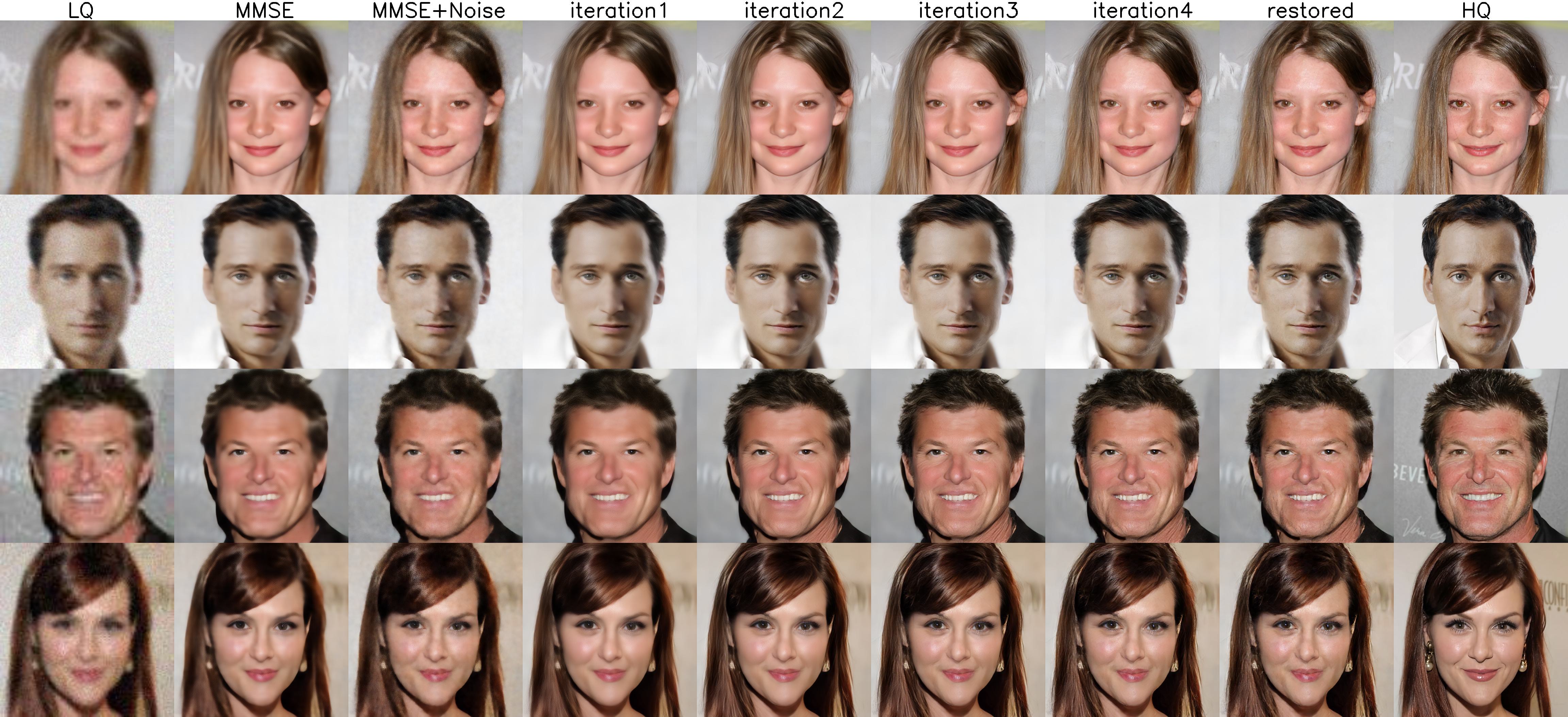
Figure 11: Visual steps of ELIR . Illustrations of the restoration process, visualizing the process from LQ images to visually appealing results. Here, we utilize the Latent MMSE estimator and $K=5$ multi-segment of Latent CFM. The images are sampled from CelebA-Test for blind face restoration.

ELIR steps. To evaluate ELIR ’s performance in latent space, Table LABEL:steps presents PSNR and FID values at each processing step. As expected, the highest PSNR is achieved after Latent MMSE, confirming its effectiveness. Subsequently, PSNR gradually decreases while FID improves, reflecting the expected distortion-perception trade-off. Figure 11 in the Appendix, illustrates the restoration process, visualizing the process from LQ images to visually appealing results.

Table 3: ELIR steps. ELIR steps from low-quality image (LQ) to restoration on CelebA-Test for blind face restoration. The observation of the highest PSNR after MMSE aligns with expectations and validates the effective implementation of Latent MMSE.

Step	FID($\downarrow$)	PSNR($\uparrow$)
LQ	145.29	25.26
Latent MMSE	72.57	26.43
Latent MMSE + Noise	78.91	26.20
Iteration 1	63.19	26.25
Iteration 2	55.66	25.85
Iteration 3	46.36	25.63
Iteration 4	40.21	25.56
Restored	39.75	25.55

Efficieny of Latent CFM. Figure 4 compares the performance of FM and CFM in latent space by plotting PSNR and FID for varying NFEs. Both methods exhibit a similar trend: PSNR decreases while FID improves with increasing NFE, reflecting the expected distortion-perception trade-off. While FM requires 25 NFEs to reach a comparable FID, CFM achieves the same FID with only 5 NFEs, highlighting CFM’s superior efficiency.

Figure 4: Efficieny of LCFM. PSNR and FID are evaluated in several NFEs for Latent FM and Latent CFM for blind face restoration.

Model Size. Figure 5 presents different model sizes for super-resolution. We vary the vector field size while keeping the latent MMSE constant. Our results indicate a diminishing return in FID improvement beyond 27M parameters. For additional metrics see Table 7 in the Appendix.

Figure 5: Model Size. FID and FPS are evaluated for several model sizes on CelebA-Test for super-resolution. The area of each circle is proportional to the model size.

Effectiveness of trainable encoder. This ablation study demonstrates the importance of fine-tuning the encoder. Given that the encoder was initially trained on HQ images, it struggles to represent the LQ images encountered in various tasks. This limitation is evident in Table 4, where fixed encoders exhibit significantly lower performance, with PSNR values 1.5-2 dB lower and FID scores 2-3 points higher compared to trainable encoders. Additional metrics can be found in the Appendix (Table 8).

Table 4: Effectiveness of trainable encoder. Experiments of ELIR for denoising and inpainting on the CelebA-Test dataset w/ and w/o training the encoder.

Task	Trainable Encoder	FID($\downarrow$)	PSNR($\uparrow$)
	✗	40.89	26.55
Denoising	✓	39.73	27.13
	✗	43.00	23.46
Inpainting	✓	40.17	25.40

6 Conclusions

This study introduces Efficient Latent Image Restoration (ELIR), an efficient IR method that operates within the latent space. ELIR consists of two stages: latent MMSE estimator, whose goal is to estimate the latent presentation of a clean image, followed by latent consistency flow matching (LCFM). The LCFM is a combination of latent flow matching and consistency flow matching that enables a small number of NFEs and a reduction of the evaluation cost. In addition, we propose an efficient neural network to significantly reduce computational complexity and model size. We have evaluated ELIR on several IR tasks and shown state-of-the-art performance in terms of model efficiency. In terms of distortion and perceptual quality, we have shown competitive results with state-of-the-art methods. This makes ELIR an efficient image restoration method that can be deployed on resource-constrained edge devices while maintaining competitive performance with state-of-the-art methods.

7 Appendix

Table of Contents:

• Neural Network Architecture: A description of the Neural Network Architecture can be found in Appendix  7.1

• Hyperparameters: Details on the hyperparameters used in the experiments are provided in Appendix  7.2.

• Additional Results: Further results can be found in Appendix  7.3.

• Additional Ablations: Additional ablations are shown in Appendix  7.4

7.1 Neural Network Architecture

To achieve a lightweight and efficient model, we utilize Tiny AutoEncoder (von Platen et al., 2022), a pre-trained tiny CNN version of Stable Diffusion 3 VAE (Esser et al., 2024). Tiny AutoEncoder allows us to lower the image dimensions into $CHW=(16,64,64)$ with only 1.2M parameters for each encoder and decoder. Given the memory and latency constraints, we restrict our architecture to convolutional layers only, eschewing transformers’ global attention mechanisms. Linear operations such as convolution can be modeled as matrix multiplication with a little overhead. As a result, these operations are highly optimized on most hardware accelerators to avoid quadratic computing complexity. Although Windows attention techniques (Liang et al., 2021; Crowson et al., 2024) can be theoretically implemented with linear time complexity, practical implementation often involves data manipulation operations, including reshaping and indexing, which remain crucial considerations for efficient implementation on resource-constrained devices. Alternatively, in our method, we use only convolution layers. During training, we utilize collapsible linear blocks (Bhardwaj et al., 2022) by adding $1\times 1$ convolution after each $3\times 3$ convolution layer and expanding the hidden channel width by 4$\times$. These two linear operations are then collapsed to a single $3\times 3$ convolution layer before inference

7.1.1 Latent MMSE

Our Latent MMSE consists of 3 cascaded RRDB blocks (Wang et al., 2018) with 96 channels each. We replace the Leaky ReLU activation of the original RRDB with SiLU. The cascade is implemented with a skip connection.

7.1.2 U-Net

For implementing the vector field we use U-Net (Ronneberger et al., 2015). U-Net is an architecture with special skip connections. These skip connections help transfer lower-level information from shallow to deeper layers. Since the shallower layers often contain low-level information, these skip connections help improve the result of image restoration. Our U-Net consists of convolution layers only. It has 3 levels with channel widths of $(128,256,512)$ and depths of $(1,2,4)$. We add a first and last convolution to align the channels of the latent tensor shape. Our basic convolution layer has $3\times 3$ kernel and all activation functions are chosen to be SiLU.

7.2 Hyper-parameters

Table 5: Hyper-parameters. Training hyper-parameters for Section 5.1.

Hyper-parameter	Blind face restoration (Section 5.1.1)	Other tasks (Section 5.1.2)
Vector-field Parameters	29M	19M
Latent MMSE Parameters	5.5M	5.5M
Encoder-Decoder Parameters	2.4M	2.4M
CFM: segments ($K$)	5	3
CFM: $\Delta t$	0.05	0.05
CFM: $\alpha$	0.001	0.001
Training Epochs	400	300
Batch Size	64	128
Image Size	512x512	256x256
Training Hardware	4 H100 80GB	4 A100 40GB
Training Time	2.5 days	1 days
Optimizer	AdamW	AdamW
Learning Rate	$10^{-4}$	$2\cdot 10^{-4}$
AdamW betas	(0.9,0.999)	(0.9,0.999)
AdamW eps	$10^{-8}$	$10^{-8}$
Weight Decay	0.02	0.02
EMA Decay	0.999	0.999

7.3 Additional Results

In-The-Wild Dataset. We test our method for blind face restoration on the in-the-wild datasets: LFW-Test (Huang et al., 2007), WebPhoto-Test (Wang et al., 2021b) and CelebAdult (Wang et al., 2021b). Here, we report only non-reference perception metrics: FID, NIQE, and MUSIQ. ELIR achieve competitive results with state-of-the-art baseline methods.

Table 6: In-The-Wild Datasets Evaluation. Comparison between ELIR and baseline models for blind face restoration. Red, blue and green indicate the best, the second best, and the third best scores, respectively.

	LFW			WebPhoto			CelebAdult
Model	FID($\downarrow$)	NIQE($\downarrow$)	MUSIQ($\uparrow$)	FID($\downarrow$)	NIQE($\downarrow$)	MUSIQ($\uparrow$)	FID($\downarrow$)	NIQE($\downarrow$)	MUSIQ($\uparrow$)
CodeFormer	53.46	4.55	75.10	88.85	4.91	72.75	115.42	4.56	75.52
GFPGAN	49.51	4.49	76.38	91.69	4.81	74.73	112.72	4.35	76.39
VQFRv2	51.22	3.82	74.40	88.28	4.59	70.93	108.67	4.01	75.11
DifFace	45.34	3.80	70.04	93.01	4.02	65.77	100.78	3.69	72.12
DiffBIR	42.30	5.76	76.77	91.19	6.28	73.13	108.99	5.74	76.37
ResShift	53.85	4.18	71.12	80.14	4.33	71.47	110.06	4.22	73.43
PMRF	51.82	3.55	69.83	83.48	3.74	65.07	104.72	3.45	72.82
ELIR (Ours)	54.62	3.65	70.08	92.98	4.09	64.97	105.68	3.37	74.12

Figure 6: Visual Results for Super Resolution. Visual comparisons between ELIR and PMRF (Ohayon et al., 2024) sampled from CelebA-Test for super-resolution task.

Figure 7: Visual Results for Denoising. Visual comparisons between ELIR and PMRF (Ohayon et al., 2024) sampled from CelebA-Test for image denoising task.

Figure 8: Visual Results for Inpainting. Visual comparisons between ELIR and PMRF (Ohayon et al., 2024) sampled from CelebA-Test for inpainting task.

Figure 9: Visual Results for Colorization. Visual comparisons between ELIR and PMRF (Ohayon et al., 2024) sampled from CelebA-Test for colorization task.

7.4 Additional Ablations

Table 7: Model Size Ablation. Evaluation of various model sizes for super-resolution on the CelebA-Test dataset. Here, we fix $K=3$ and ablate only the vector field size, leaving the MMSE parameters unchanged. We note that the FID decreases as model size increases, while PSNR remains relatively constant.

	Percepual Quality			Distortion
#Params [M]	FID($\downarrow$)	NIQE($\downarrow$)	MUSIQ($\uparrow$)	PSNR($\uparrow$)	SSIM($\uparrow$)	LPIPS($\downarrow$)	FPS($\uparrow$)
13	51.69	5.02	63.44	23.87	0.6582	0.3317	48.55
17	47.33	5.00	63.96	23.85	0.6572	0.3273	48.05
27	44.81	5.01	64.06	23.87	0.6579	0.3256	47.81
37	44.71	5.01	64.26	23.86	0.6579	0.3253	42.94

Table 8: Effectiveness of trainable encoder. Experiments of ELIR for denoising and inpainting on the CelebA-Test dataset w/ and w/o training the encoder. We observe that allowing the encoder to fine-tune during training is crucial. Since the encoder was pre-trained on HQ images, it struggles to represent LQ images accurately. This leads to substantial errors that are reflected in all evaluated metrics.

		Perceptual Quality			Distortion
Task	Trainable Encoder	FID($\downarrow$)	NIQE($\downarrow$)	MUSIQ($\uparrow$)	PSNR($\uparrow$)	SSIM($\uparrow$)	LPIPS($\downarrow$)
	✗	40.89	5.18	64.99	26.55	0.7568	0.2675
Denoising	✓	39.73	5.04	66.21	27.13	0.7737	0.2537
	✗	43.00	4.96	64.56	23.46	0.6654	0.3327
Inpainting	✓	40.17	4.95	66.17	25.40	0.7302	0.2779

Model Latency. Table 9 presents ablation study for model latency. Here, we vary the multi-segment value $K$ while maintaining a fixed model size. Our findings suggest that $K=3$ provides a suitable trade-off between FID and frames per second (FPS). This ablation was conducted on the CelebA-Test dataset for the super-resolution but similar results were found in other tasks. Therefore, we set $K=3$ for super-resolution, denoising, inpainting, and colorization.

Table 9: Latency Ablation. Evaluation of a different multi-segment values ($K$) for super-resolution on the CelebA-Test dataset. Each model was trained with a fixed size of 27M parameters. We note that the FPS decreases as $K$ increases.

	Perceptual Quality			Distortion
K	FID($\downarrow$)	NIQE($\downarrow$)	MUSIQ($\uparrow$)	PSNR($\uparrow$)	SSIM($\uparrow$)	LPIPS($\downarrow$)	FPS($\uparrow$)
1	45.76	5.08	65.07	23.91	0.6612	0.3207	70.30
3	44.81	5.01	64.06	23.87	0.6579	0.3256	49.26
5	44.64	4.96	64.46	23.85	0.6573	0.3262	36.35
7	44.20	4.92	64.61	23.79	0.6548	0.3278	30.25

Latent MMSE loss space. This ablation study investigates the impact of the $\ell_{2}$ loss space on model performance. We compared the original latent-space loss from (6) with an alternative pixel-space loss:

$$\mathcal{L}_{2}\left(\bm{\phi},\bm{\omega}\right) =\mathbb{E}_{\bm{x},\bm{y}}\left[\left\lVert\mathcal{D}(g_{\bm{\phi}}(\mathcal{E}_{\bm{\omega}}\left(\bm{y}\right)))-\bm{x}\right\rVert_{2}^{2}\right].$$ (11)

Table 10 demonstrates a trade-off between PSNR and perceptual quality. While pixel-space losses generally achieve higher PSNR values, they often result in lower perceptual quality, leading to visually less appealing restored images.

Table 10: Latent MMSE Loss space. Experiments across different tasks reveal that pixel space loss generally yields higher PSNR values than latent space loss. However, this often comes at the cost of reduced perceptual quality, leading to less visually appealing restored images.

		Perceptual Quality			Distortion
Task	Loss Space	FID($\downarrow$)	NIQE($\downarrow$)	MUSIQ($\uparrow$)	PSNR($\uparrow$)	SSIM($\uparrow$)	LPIPS($\downarrow$)
	latent	39.75	4.07	71.45	25.55	0.6933	0.3753
blind face restoration	pixel	40.77	4.22	68.66	25.88	0.7035	0.3762
	latent	44.81	5.01	64.06	23.87	0.6579	0.3256
super resolution	pixel	48.94	4.96	62.67	24.03	0.6644	0.3300
	latent	39.73	5.04	66.21	27.13	0.7737	0.2537
denoising	pixel	39.80	4.97	66.06	27.27	0.7766	0.2582
	latent	40.17	4.95	66.17	25.40	0.7302	0.2779
inpainting	pixel	40.34	4.92	65.18	25.70	0.7414	0.2782
	latent	46.34	4.91	65.12	22.83	0.7303	0.3705
colorization	pixel	49.71	4.88	63.61	22.90	0.7338	0.3834

Latent MMSE vs SwinIR. This ablation study analyzes our Latent MMSE approach by comparing it to both pixel and latent estimators of SwinIR (Liang et al., 2021). Maintaining a constant model size, Table 11 presents the comparison results. In the latent space, our method exhibits performance comparable to SwinIR. While SwinIR in pixel space achieves higher PSNR values, our approach demonstrates a better FID score. Notably, our convolution-based Latent MMSE shows a much higher frame per second (FPS). These evaluations were conducted on the CelebA-Test dataset for blind face restoration. Note that the latent SwinIR implementation utilizes a window size of $4\times 4$.

Table 11: Latent MMSE vs SwinIR. We compared our Latent MMSE approach with the pixel and latent estimators of SwinIR (Liang et al., 2021). Our method demonstrated comparable performance to SwinIR while achieving a significant improvement in frame rate (FPS).

MMSE		Perceptual Quality			Distortion
Arch	Latent	FID($\downarrow$)	NIQE($\downarrow$)	MUSIQ($\uparrow$)	PSNR($\uparrow$)	SSIM($\uparrow$)	LPIPS($\downarrow$)	#Params[M]	FPS($\uparrow$)
CNN	✓	39.75	4.07	71.45	25.55	0.6933	0.3753	37	19.51
SwinIR	✓	39.81	3.99	72.21	25.59	0.6938	0.3695	37	13.22
SwinIR	✗	41.31	4.01	70.19	25.96	0.6980	0.3733	37	9.80

Noise Level ablation. This ablation study investigates the impact of noise level $\sigma_{s}$ on model performance. Additive noise is vital for learning the complex dynamics of image degradation, enabling the generation of high-quality images. However, careful tuning of $\sigma_{s}$ is essential; excessive noise can lead to distortion, while insufficient noise may degrade perceptual quality. Table 12 presents the results for various $\sigma_{s}$ values. Based on these results, $\sigma_{s}=0.1$ appears to offer the best balance between minimizing distortion and maintaining high perceptual quality. Therefore, we set $\sigma_{s}=0.1$ in our experiments. This ablation was conducted on the CelebA-Test dataset for the super-resolution but similar results were found in other tasks.

Table 12: Noise Level ablation. Experiments across several noise levels $\sigma_{s}=\{0.05,0.1,0.2\}$. $\sigma_{s}=0.1$ appears to provide a suitable trade-off between distortion and perceptual quality.

	Perceptual Quality			Distortion
$\sigma_{s}$	FID($\downarrow$)	NIQE($\downarrow$)	MUSIQ($\uparrow$)	PSNR($\uparrow$)	SSIM($\uparrow$)	LPIPS($\downarrow$)
0.05	48.07	5.17	63.42	24.06	0.6649	0.3229
0.1	44.81	5.01	64.06	23.87	0.6579	0.3256
0.2	43.40	4.90	64.91	23.54	0.6480	0.3312

Time Interval ablation. In this ablation study, we investigate the influence of the time interval ($\Delta t$) on model performance. Table 13 presents the results obtained for several $\Delta t$ values. Reducing $\Delta t$ is expected to enhance FID scores, however, it may also lead to an increase in distortion metrics. This study aims to identify the $\Delta t$ value that minimizes distortion while maintaining a high level of perceptual quality. According to the results, $\Delta t=0.05$ offers the most favorable balance between minimizing distortion and preserving perceptual quality. This ablation was conducted on the CelebA-Test dataset for the image denoising but similar results were found in other tasks.

Table 13: Time interval ablation. Experiments across several time interval $\Delta t=\{0.01,0.05,0.1\}$. $\Delta t=0.05$ appears to provide a suitable trade-off between distortion and perceptual quality.

	Perceptual Quality			Distortion
$\Delta t$	FID($\downarrow$)	NIQE($\downarrow$)	MUSIQ($\uparrow$)	PSNR($\uparrow$)	SSIM($\uparrow$)	LPIPS($\downarrow$)
0.01	39.68	4.92	66.47	27.03	0.7699	0.2589
0.05	39.73	5.04	66.21	27.13	0.7737	0.2537
0.1	41.26	5.26	65.43	27.18	0.7764	0.2521

CFM trajectories. Latent CFM improves the flow straightness by enforcing consistency within the velocity field, which reduces discretization errors. Figure 10 illustrates the “straitness” of the trajectories in the latent space. However, when these trajectories are projected back to the pixel space, this property is not preserved due to the decoder’s non-linearity.

Figure 10: CFM trajectories. The left figure visualizes CFM trajectories in latent space, connecting flow from source (p0) to target point (p1). These trajectories exhibit “straight” flows along two latent variables, a consequence of the Latent CFM operating within the latent space. However, this linearity is not preserved when projected into pixel space due to the decoder’s non-linearity, as demonstrated in the right figure.

References

- Albergo & Vanden-Eijnden (2023) Albergo, M. S. and Vanden-Eijnden, E. Building normalizing flows with stochastic interpolants. In The Eleventh International Conference on Learning Representations ICLR. OpenReview.net, 2023.
- Bhardwaj et al. (2022) Bhardwaj, K., Milosavljevic, M., O’Neil, L., Gope, D., Matas, R., Chalfin, A., Suda, N., Meng, L., and Loh, D. Collapsible linear blocks for super-efficient super resolution. Proceedings of Machine Learning and Systems, 4:529–547, 2022.
- Blau & Michaeli (2018) Blau, Y. and Michaeli, T. The perception-distortion tradeoff. In Proceedings of the IEEE conference on computer vision and pattern recognition, pp. 6228–6237, 2018.
- Chen & Mo (2022) Chen, C. and Mo, J. IQA-PyTorch: Pytorch toolbox for image quality assessment. [Online]. Available: https://github.com/chaofengc/IQA-PyTorch, 2022.
- Chen et al. (2018) Chen, R. T., Rubanova, Y., Bettencourt, J., and Duvenaud, D. K. Neural ordinary differential equations. Advances in neural information processing systems, 31, 2018.
- Crowson et al. (2024) Crowson, K., Baumann, S. A., Birch, A., Abraham, T. M., Kaplan, D. Z., and Shippole, E. Scalable high-resolution pixel-space image synthesis with hourglass diffusion transformers. In Forty-first International Conference on Machine Learning, 2024. URL https://openreview.net/forum?id=WRIn2HmtBS.
- Dao et al. (2023) Dao, Q., Phung, H., Nguyen, B., and Tran, A. Flow matching in latent space. arXiv preprint arXiv:2307.08698, 2023.
- Dong et al. (2015) Dong, C., Loy, C. C., He, K., and Tang, X. Image super-resolution using deep convolutional networks. IEEE transactions on pattern analysis and machine intelligence, 38(2):295–307, 2015.
- Dong et al. (2012) Dong, W., Zhang, L., Shi, G., and Li, X. Nonlocally centralized sparse representation for image restoration. IEEE transactions on Image Processing, 22(4):1620–1630, 2012.
- Esser et al. (2024) Esser, P., Kulal, S., Blattmann, A., Entezari, R., Müller, J., Saini, H., Levi, Y., Lorenz, D., Sauer, A., Boesel, F., et al. Scaling rectified flow transformers for high-resolution image synthesis. In Forty-first International Conference on Machine Learning, 2024.
- Fei et al. (2023) Fei, B., Lyu, Z., Pan, L., Zhang, J., Yang, W., Luo, T., Zhang, B., and Dai, B. Generative diffusion prior for unified image restoration and enhancement. In Proceedings of the IEEE/CVF Conference on Computer Vision and Pattern Recognition, pp. 9935–9946, 2023.
- Freirich et al. (2021) Freirich, D., Michaeli, T., and Meir, R. A theory of the distortion-perception tradeoff in wasserstein space. In Beygelzimer, A., Dauphin, Y., Liang, P., and Vaughan, J. W. (eds.), Advances in Neural Information Processing Systems, 2021. URL https://openreview.net/forum?id=qeaT2O5fNKC.
- Goodfellow et al. (2014) Goodfellow, I., Pouget-Abadie, J., Mirza, M., Xu, B., Warde-Farley, D., Ozair, S., Courville, A., and Bengio, Y. Generative adversarial nets. Advances in neural information processing systems, 27, 2014.
- Gu et al. (2022) Gu, Y., Wang, X., Xie, L., Dong, C., Li, G., Shan, Y., and Cheng, M.-M. Vqfr: Blind face restoration with vector-quantized dictionary and parallel decoder. In European Conference on Computer Vision, pp. 126–143. Springer, 2022.
- Heusel et al. (2017) Heusel, M., Ramsauer, H., Unterthiner, T., Nessler, B., and Hochreiter, S. Gans trained by a two time-scale update rule converge to a local nash equilibrium. Advances in neural information processing systems, 30, 2017.
- Ho et al. (2020) Ho, J., Jain, A., and Abbeel, P. Denoising diffusion probabilistic models. Advances in neural information processing systems, 33:6840–6851, 2020.
- Huang et al. (2007) Huang, G. B., Ramesh, M., Berg, T., and Learned-Miller, E. Labeled faces in the wild: A database for studying face recognition in unconstrained environments. Technical Report 07-49, University of Massachusetts, Amherst, October 2007.
- Karras et al. (2019) Karras, T., Laine, S., and Aila, T. A style-based generator architecture for generative adversarial networks. In Proceedings of the IEEE/CVF conference on computer vision and pattern recognition, pp. 4401–4410, 2019.
- Kawar et al. (2022) Kawar, B., Elad, M., Ermon, S., and Song, J. Denoising diffusion restoration models. Advances in Neural Information Processing Systems, 35:23593–23606, 2022.
- Ke et al. (2021) Ke, J., Wang, Q., Wang, Y., Milanfar, P., and Yang, F. Musiq: Multi-scale image quality transformer. In Proceedings of the IEEE/CVF international conference on computer vision, pp. 5148–5157, 2021.
- Kupyn et al. (2019) Kupyn, O., Martyniuk, T., Wu, J., and Wang, Z. Deblurgan-v2: Deblurring (orders-of-magnitude) faster and better. In Proceedings of the IEEE/CVF international conference on computer vision, pp. 8878–8887, 2019.
- Li et al. (2020) Li, X., Chen, C., Zhou, S., Lin, X., Zuo, W., and Zhang, L. Blind face restoration via deep multi-scale component dictionaries. In European conference on computer vision, pp. 399–415. Springer, 2020.
- Li et al. (2023) Li, Y., Hu, J., Wen, Y., Evangelidis, G., Salahi, K., Wang, Y., Tulyakov, S., and Ren, J. Rethinking vision transformers for mobilenet size and speed. In Proceedings of the IEEE international conference on computer vision, 2023.
- Liang et al. (2021) Liang, J., Cao, J., Sun, G., Zhang, K., Van Gool, L., and Timofte, R. Swinir: Image restoration using swin transformer. In Proceedings of the IEEE/CVF international conference on computer vision, pp. 1833–1844, 2021.
- Lin et al. (2023) Lin, X., He, J., Chen, Z., Lyu, Z., Dai, B., Yu, F., Ouyang, W., Qiao, Y., and Dong, C. Diffbir: Towards blind image restoration with generative diffusion prior. arXiv preprint arXiv:2308.15070, 2023.
- Lipman et al. (2023) Lipman, Y., Chen, R. T. Q., Ben-Hamu, H., Nickel, M., and Le, M. Flow matching for generative modeling. In The Eleventh International Conference on Learning Representations, 2023. URL https://openreview.net/forum?id=PqvMRDCJT9t.
- Liu et al. (2023) Liu, X., Gong, C., and qiang liu. Flow straight and fast: Learning to generate and transfer data with rectified flow. In The Eleventh International Conference on Learning Representations, 2023. URL https://openreview.net/forum?id=XVjTT1nw5z.
- Liu et al. (2015) Liu, Z., Luo, P., Wang, X., and Tang, X. Deep learning face attributes in the wild. In Proceedings of International Conference on Computer Vision (ICCV), December 2015.
- (29) Loshchilov, I. and Hutter, F. Decoupled weight decay regularization. In International Conference on Learning Representations.
- Luo et al. (2020) Luo, Z., Huang, Y., Li, S., Wang, L., and Tan, T. Unfolding the alternating optimization for blind super resolution. Advances in Neural Information Processing Systems (NeurIPS), 33, 2020.
- Mittal et al. (2012) Mittal, A., Soundararajan, R., and Bovik, A. C. Making a “completely blind” image quality analyzer. IEEE Signal processing letters, 20(3):209–212, 2012.
- Ohayon et al. (2024) Ohayon, G., Michaeli, T., and Elad, M. Posterior-mean rectified flow: Towards minimum mse photo-realistic image restoration. arXiv preprint arXiv:2410.00418, 2024.
- Rombach et al. (2022) Rombach, R., Blattmann, A., Lorenz, D., Esser, P., and Ommer, B. High-resolution image synthesis with latent diffusion models. In Proceedings of the IEEE/CVF conference on computer vision and pattern recognition, pp. 10684–10695, 2022.
- Ronneberger et al. (2015) Ronneberger, O., Fischer, P., and Brox, T. U-net: Convolutional networks for biomedical image segmentation. In Medical image computing and computer-assisted intervention–MICCAI 2015: 18th international conference, Munich, Germany, October 5-9, 2015, proceedings, part III 18, pp. 234–241. Springer, 2015.
- Sohl-Dickstein et al. (2015) Sohl-Dickstein, J., Weiss, E., Maheswaranathan, N., and Ganguli, S. Deep unsupervised learning using nonequilibrium thermodynamics. In International conference on machine learning, pp. 2256–2265. PMLR, 2015.
- Song et al. (2021) Song, J., Meng, C., and Ermon, S. Denoising diffusion implicit models. In International Conference on Learning Representations, 2021. URL https://openreview.net/forum?id=St1giarCHLP.
- von Platen et al. (2022) von Platen, P., Patil, S., Lozhkov, A., Cuenca, P., Lambert, N., Rasul, K., Davaadorj, M., Nair, D., Paul, S., Berman, W., Xu, Y., Liu, S., and Wolf, T. Diffusers: State-of-the-art diffusion models. https://github.com/huggingface/diffusers, 2022.
- (38) Wang, X., Xie, L., Dong, C., and Shan, Y. Real-esrgan: Training real-world blind super-resolution with pure synthetic data. In International Conference on Computer Vision Workshops (ICCVW).
- Wang et al. (2018) Wang, X., Yu, K., Wu, S., Gu, J., Liu, Y., Dong, C., Qiao, Y., and Change Loy, C. Esrgan: Enhanced super-resolution generative adversarial networks. In Proceedings of the European conference on computer vision (ECCV) workshops, pp. 0–0, 2018.
- Wang et al. (2021a) Wang, X., Li, Y., Zhang, H., and Shan, Y. Towards real-world blind face restoration with generative facial prior. In The IEEE Conference on Computer Vision and Pattern Recognition (CVPR), 2021a.
- Wang et al. (2021b) Wang, X., Li, Y., Zhang, H., and Shan, Y. Towards real-world blind face restoration with generative facial prior. In Proceedings of the IEEE/CVF conference on computer vision and pattern recognition, pp. 9168–9178, 2021b.
- Wang et al. (2023) Wang, Y., Yu, J., and Zhang, J. Zero-shot image restoration using denoising diffusion null-space model. In The Eleventh International Conference on Learning Representations, 2023.
- Wang et al. (2004) Wang, Z., Bovik, A. C., Sheikh, H. R., and Simoncelli, E. P. Image quality assessment: from error visibility to structural similarity. IEEE transactions on image processing, 13(4):600–612, 2004.
- Whang et al. (2022) Whang, J., Delbracio, M., Talebi, H., Saharia, C., Dimakis, A. G., and Milanfar, P. Deblurring via stochastic refinement. In Proceedings of the IEEE/CVF Conference on Computer Vision and Pattern Recognition, pp. 16293–16303, 2022.
- Yang et al. (2024) Yang, L., Zhang, Z., Zhang, Z., Liu, X., Xu, M., Zhang, W., Meng, C., Ermon, S., and Cui, B. Consistency flow matching: Defining straight flows with velocity consistency. arXiv preprint arXiv:2407.02398, 2024.
- Yang et al. (2021) Yang, T., Ren, P., Xie, X., and Zhang, L. Gan prior embedded network for blind face restoration in the wild. In Proceedings of the IEEE/CVF conference on computer vision and pattern recognition, pp. 672–681, 2021.
- Yue & Loy (2024) Yue, Z. and Loy, C. C. Difface: Blind face restoration with diffused error contraction. IEEE Transactions on Pattern Analysis and Machine Intelligence, 2024.
- Yue et al. (2024) Yue, Z., Wang, J., and Loy, C. C. Efficient diffusion model for image restoration by residual shifting. IEEE Transactions on Pattern Analysis and Machine Intelligence, pp. 1–15, 2024. doi: 10.1109/TPAMI.2024.3461721.
- Zhang et al. (2018a) Zhang, K., Zuo, W., and Zhang, L. Learning a single convolutional super-resolution network for multiple degradations. In IEEE Conference on Computer Vision and Pattern Recognition, pp. 3262–3271, 2018a.
- Zhang et al. (2021) Zhang, K., Liang, J., Van Gool, L., and Timofte, R. Designing a practical degradation model for deep blind image super-resolution. In Proceedings of the IEEE/CVF International Conference on Computer Vision, pp. 4791–4800, 2021.
- Zhang et al. (2018b) Zhang, R., Isola, P., Efros, A. A., Shechtman, E., and Wang, O. The unreasonable effectiveness of deep features as a perceptual metric. In CVPR, 2018b.
- Zhou et al. (2022) Zhou, S., Chan, K. C., Li, C., and Loy, C. C. Towards robust blind face restoration with codebook lookup transformer. In NeurIPS, 2022.
- Zhu et al. (2024) Zhu, Y., Zhao, W., Li, A., Tang, Y., Zhou, J., and Lu, J. Flowie: Efficient image enhancement via rectified flow. In Proceedings of the IEEE/CVF Conference on Computer Vision and Pattern Recognition, pp. 13–22, 2024.