Integral Fast Fourier Color Constancy

Abstract

Traditional auto white balance (AWB) algorithms typically assume a single global illuminant source, which leads to color distortions in multi-illuminant scenes. While recent neural network-based methods have shown excellent accuracy in such scenarios, their high parameter count and computational demands limit their practicality for real-time video applications. The Fast Fourier Color Constancy (FFCC) algorithm was proposed for single-illuminant-source scenes, predicting a global illuminant source with high efficiency. However, it cannot be directly applied to multi-illuminant scenarios unless specifically modified. To address this, we propose Integral Fast Fourier Color Constancy (IFFCC), an extension of FFCC tailored for multi-illuminant scenes. IFFCC leverages the proposed integral UV histogram to accelerate histogram computations across all possible regions in Cartesian space and parallelizes Fourier-based convolution operations, resulting in a spatially-smooth illumination map. This approach enables high-accuracy, real-time AWB in multi-illuminant scenes. Extensive experiments show that IFFCC achieves accuracy that is on par with or surpasses that of pixel-level neural networks, while reducing the parameter count by over $400\times$ and processing speed by $20-100\times$ faster than network-based approaches.

1 Introduction

Color constancy is a fundamental property of the human visual system, allowing for consistent color perception despite changes in illumination chromaticity. While this ability may seem “natural” to the human eye and visual cortex, replicating it in computational imaging systems is a complex challenge [22, 19]. Auto white balance (AWB) in image signal processing (ISP) is thus essential for approximating human-like color constancy by estimating ambient illumination chromaticity, enabling accurate color reproduction across varied lighting conditions.

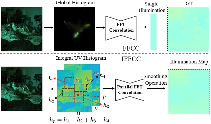
Figure 1: Frameworks comparison between IFFCC and FFCC (top). FFCC uses a global histogram to predict a single illuminant, limiting its application in multi-illuminant scenes. In contrast, IFFCC utilizes an integral UV histogram for efficient region-specific histogram computation, generating spatially continuous illumination map through parallelized Fast Fourier convolution and smoothing to achieve high-accuracy, real-time auto white balance in multi-illuminant scenarios.

Traditional white balance methods often assume the presence of a single dominant illumination and rely on statistical algorithms [18, 45, 21, 23], such as the gray world algorithm [10] and the white patch algorithm [33] etc., to estimate the scene illumination. These algorithms may also be machine learning-based, trained on AWB benchmarks [27, 3]. However, they frequently bear local color distortion in complex multi-illuminant environments, as a single white balance adjustment is inadequate to handle varying lighting conditions. For instance, a room illuminated by both warm high pressure sodium lighting and cool window light may still fail to accurately reproduce the scene’s true colors.

Recently, deep neural network-based algorithms have been widely applied to pixel-level multi-illuminant prediction tasks [11, 31, 45, 34], utilizing deep learning to achieve accurate illumination map estimation in complex scenes. These methods are especially effective in capturing edge-aware, spatial illumination variations. However, the high parameter counts and computational demands of these models create substantial challenges for deployment in real-time, resource-limited applications, such as mobile photography devices. Beyond achieving high pixel-level prediction accuracy, a practical local AWB solution from an industrial perspective should prioritize several key requirements:

Effectiveness - The algorithm can accomplish the AWB task up to a high accuracy, in any given spatial region, ensuring robust performance in a wide range of scenarios and including different light intensities and color temperatures.

Efficiency - White balance adjustments must be fast enough to provide immediate feedback during view-finding and capture, particularly in rapidly changing lighting. Limited camera resources require AWB, along with other ISP functions like AE, AF, and color correction, to operate in real time. On resource-constrained devices like smartphones, low computational complexity and memory usage are essential, with AWB processing times ideally under 10 ms.

Thumbnail Input or Stat - Many color constancy algorithms require full-resolution, high-bit images, which is resource-intensive on pervasive mobile devices. For the purpose of real-time preview, the module for generating AWB stat is often realized in hardware (like DSP), outputting a thumbnail-sized input (e.g., $64\times 48$, 8-bit).

Smoothness - The algorithm should maintain stable performance under varying lighting conditions, avoiding artifacts or abrupt transitions, and ensure smooth, accurate white balance across entire images or video frames.

The FFCC algorithm [3] effectively meets the requirements for global illumination scenarios but faces challenges in multi-illuminant scenes. Specifically, FFCC requires repeated histogram extraction for each target region, significantly increasing processing time and limiting its suitability for real-time applications, especially on resource-constrained devices like smartphones. Additionally, FFCC lacks mechanisms to ensure smooth spatial transitions under rapidly changing lighting, which can result in abrupt shifts in white balance.

To overcome FFCC’s limitations in multi-illuminant scenarios, we propose Integral Fast Fourier Color Constancy (IFFCC), a local extension of FFCC [3] designed for white balance in complex lighting conditions, as shown in Fig. 1. IFFCC achieves speeds $20-100\times$ faster than other local methods, with a runtime of 5.8 ms for $64\times 48$ preview images on a CPU. Building upon FFCC, IFFCC introduces several key contributions:

1. IFFCC outperforms prior-arts traditional algorithms and most network-based methods in multi-light source scenarios, achieving performance comparable to the best network-based methods;

2. IFFCC leverages the proposed integral UV histogram to accelerate histogram extraction across all possible regions in Cartesian space. It efficiently computes the histogram for any region using only a few simple arithmetic operations, ensuring both high accuracy and real-time performance for multi-illuminant white balance.

3. IFFCC is spatially adaptive: spatial interpolation and filtering on local estimates ensure smooth transitions while preserving distinct light boundaries and sharp gradients, enabling precise, pixel-level color correction.

2 Related Work

2.1 Global AWB Methods

Conventional methods have long served as foundational approaches for uniform color constancy. These techniques estimate the illuminant’s color based on the statistical characteristics of a single lighting source in the image [9, 17, 18, 21, 23, 47]. Notable single-illumination examples include the Gray World assumption [10], which posits that the average color of a scene under equal-energy white illumination should appear gray. Similarly, White Patch [33] assumes that the brightest pixel serves as a hint for illumination chromaticity. Refining these assumptions to focus on local patches or higher-order gradients has led to more robust statistics-based methods, optimized for more-challenging global ambient illuminations. These methods include General Gray World [1], Gray Edge [47], Shades-of-Gray [16], and LSRS [20], among others [11, 42].

In same context, more machine learning-based methods have been proposed, such as learning-based kernels [3, 2], convolutional feature extraction [6, 27], and other machine learning approaches have been devised specifically for handling single-illumination scenarios [48, 41, 43, 36, 35]. The most closely related methods to ours are Barron’s CCC [2] and FFCC [3]. CCC reformulates color constancy as a color localization task in log-chromaticity space, using convolutional kernels to accurately locate the correct color. FFCC builds on this by applying the Fast Fourier Transform on a chromaticity torus, greatly improving the speed and accuracy of chromaticity estimation. However, both are global methods and lack direct applicability to local scenes unless explicitly provided with a local window.

2.2 Local AWB Methods

Several multi-illuminant benchmarks have been introduced [24, 31, 4, 5, 8, 39, 35], with various methods proposed to tackle local white balance. These methods often rely on additional prior information or metadata, such as the number of light sources [4, 26] or facial regions of interest [5]. For instance, [28] uses flash photography to achieve local white balance. A novel framework in [4] treats the problem as an energy minimization task within a conditional random field, leveraging local light source estimates. [8] employs a global method with spatial variation, while [7] introduces a CNN framework based on sliding windows. Additionally, [46] applies a generative adversarial network (GAN) to correct images using synthetic datasets, adjusting the color based on the lighting information. More recently, Domislović et al. [14] proposed extracting spatial features for illumination prediction on each patch, and AID [32] introduces a deep model utilizing slot attention [37] to generate chromaticity and weight maps for each light source, with the added benefit of allowing user edits.

Among these approaches, most focus on pixel-level predictions, typically using encoder-decoder architectures (e.g., U-Net) to capture fine-grained illumination chromaticity details. However, this approach presents several practical challenges: Pixel-level prediction is computationally expensive and can lead to inconsistent results, particularly for high-resolution images, which limits real-time applicability. Additionally, pixel-level color correction may overlook important illumination chromaticity differences that are crucial for accurately rendering color-related edges. As a result, these methods may be less suitable for practical applications or mobile deployment, where computational resources are limited.

3 Method

We propose the Integral Fast Fourier Color Constancy (IFFCC) model, which builds upon the foundations of Fast Fourier Color Constancy (FFCC) [3]. Drawing inspiration from [40], we implement an histogram search for all possible target regions in image data within Cartesian coordinate space. This enables efficient retrieval of any region’s histogram in linear computation time, avoiding redundant summation operations.

FFCC Foundation. Consider a linear image stat $I$ obtained from the camera, where there are no saturated pixels and the black level has been subtracted. Assuming the RGB value of any pixel is the product of its true albedo RGB value $W$ and the uniform illumination value shared across all pixels: $I=W\times L$. Although this assumption disregards shadows, dichromatic reflections, and spatial variations, it remains effective and widely accepted. Our aim is to estimate the $L$ given $I$, and then $W=I/L$.

For an input RGB image $I$, CCC [2] defines two log-chroma measures for each pixel $i$:

$$u^{(i)}=\log(I_{g}^{(i)}/I_{r}^{(i)})\quad v^{(i)}=\log(I_{g}^{(i)}/I_{b}^{(i)})$$ (1)

Neglecting the absolute scaling of $W$, the estimation of $L$ is then simplified as $L_{u}=\log(L_{g}/L_{r})\quad L_{v}=\log(L_{g}/L_{b})$. Given the unknown absolute scale, the inverse mapping from RGB to UV is challenging. To simplify the recovery process, we assume $L$ is the unit-norm:

$$L_{r}= {\exp(-L_{u})}/{z}\quad L_{g}={1}/{z}\quad L_{b}={\exp(-L_{v})}/{z}$$ (2)

$$z=\sqrt{\exp(-L_{u})^{2}+\exp(-L_{v})^{2}+1}$$

This logarithmic chromatic space method has several advantages over the RGB approach. First, it involves only two unknowns instead of three, which enhances numerical stability. Additionally, this framework transforms the multiplicative constraints related to $W$ and $I$ into additive constraints [15], effectively converting the color constancy task into a positioning task in a two-dimensional space.

Following FFCC, we use FFT-based convolution in the log-chroma space, leveraging its periodicity to accelerate computations. Given the histogram’s limited size, which does not fully capture the range of colors in natural images, a modular algorithm is needed to allow pixels to ”wrap around” in this space:

$$H(x,y)= \sum_{i}\left(\mod\left({(u^{(i)}-u_{s})}/{b}-x,n\right)<1\right.$$ (3)

$$\quad\left.\wedge\mod\left({(v^{(i)}-v_{s})}/{b}-y,n\right)<1\right)$$

where $H(x,y)$ represents the count of pixels in $I$ whose log-chroma coordinates are close to the $(u,v)$ coordinates associated with the histogram position $(x,y)$, $n$ is the number of bins, and $b$ is the bin size. $u_{s}$ and $v_{s}$ denote the starting positions of $u$ and $v$, respectively. The operations here differ from those in CCC. In this case, the $(x,y)$ positions in the histogram no longer represent absolute colors, but rather a set of $(u,v)$ color coordinates. The filtered results produce a set of light sources, from which we apply the “gray light de-aliasing” method to resolve the resulting light source clusters. This method assumes that the light sources are as close as possible to the center of the histogram.

FFCC employs the Differentiable Bivariate von Mises (BVM) [38] method to address the single estimation of light sources from the toroidal PDF. Unlike FFCC, we need to predict multiple light sources for each image. Therefore, the BVM method is parallelized across multiple windows to predict several light sources simultaneously, as described in Section 3.3. The final convolutional structure is as follows:

$$P=\text{softmax}(B+M\circ\sum_{s}H_{s}\ast F_{s})$$ (4)

where $B$ is the bias map, $M$ is the learnable gain map, and $\{F_{s}\}$ is the set of learnable filters convolved with the edge-enhanced histogram group $\{H_{s}\}$.

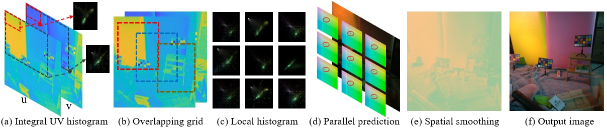
Figure 2: Overview of the IFFCC process for predicting multi-illuminant scenes. We precompute the integral UV histogram of the input image in the log-chroma space (a). Multiple target regions are extracted on the integrated UV histogram with the overlapping grid (b), and the local log-chroma histogram (c) corresponding to each region is computed using simple arithmetic operations on the UV histogram. Each histogram forms a torus that can be unfolded, producing a cluster of potential light sources. A de-aliasing step selects the most likely light source for each region (d), represented by a point within an ellipse, where the ellipse indicates IFFCC’s covariance output. Final light estimates are smoothed through interpolation and guided filtering, creating a continuous illumination map (e) that combines with the input to produce a white-balanced image (f) for multi-illuminant scenes.

3.1 Integral UV Histogram

FFCC predicts a global illumination for the image. However, when multiple illuminations are anticipated for different target regions, the process requires FFCC to repeatedly extract histograms from these various areas, significantly increasing computational load and processing time. Inspired by the work of [40], we efficiently compute the histograms for all potential regions within a given image using Cartesian coordinates. By leveraging the spatial positions of data in this coordinate system, we propagate a function starting from the origin to navigate through the remaining positions. The histogram for the current point is then updated based on the histograms of previously processed points. Once the integral histogram for each data point is obtained, the histogram for the target region can be derived using simple addition and subtraction operations. This method eliminates the need to reconstruct separate histograms for each region individually. As a result, this efficient approach significantly reduces computational overhead and improves processing time, enabling rapid analysis of multiple areas within the image.

After transforming the image into log-chroma space by Eq.1, we define the integral uv histogram as follows:

$$H_{\text{Integral}}(x^{n},b)=\bigcup_{m=0}^{n}B(u,v)^{m}$$ (5)

$$B(u,v)=\left(\begin{aligned} &\mod\left(\text{round}\left(\frac{u-u_{s}}{b}\right),n\right),\\ &\mod\left(\text{round}\left(\frac{v-v_{s}}{b}\right),n\right)\end{aligned}\right)$$ (6)

where $x^{n}$ is a sequence of points $x^{0},x^{1},\dots,x^{n}$. $B(.)$ represents the corresponding bin for the current data point, $\bigcup$ denotes the union operator, and the value of bin $b$ in $H_{\text{Integral}}(x^{n},b)$ is the sum of the histogram values of bin $b$ from all previously traversed data points. The integral histogram can also be expressed recursively as follows:

$$H_{\text{Integral}}(x^{m},b)=H_{\text{Integral}}(x^{m-1},b)\bigcup B(u,v)^{m}$$ (7)

where at the initial data point, $H_{\text{Integral}}(0,b)=0$.

In log-chroma space, updating the histogram at the current point requires the histograms of the data points above, the left, and the top-left of the current point. These three histograms have already been calculated in previous scans, so only three simple arithmetic operations are needed to update the histogram for the current point. Afterward, the bin value $b$ for the current point is calculated, and the histogram is updated accordingly. Before each propagation step, all scanned bin values are copied to the current bin values, which can be efficiently handled through fast hardware or pointer operations.

For an RGB image converted to $N_{1}\times N_{2}\times 2$ log-chroma space data, the integral histogram propagated via wavefront scanning from the top-left starting point can be written as:

$$H_{\text{Integral}}(u, v,b)=H_{\text{Integral}}(u-1,v,b)$$ (8)

$$+H_{\text{Integral}}(u,v-1,b)$$

$$-H_{\text{Integral}}(u-1,v-1,b)+B(u,v)$$

where $(u,v)$ is the coordinate of the log-chroma space. In our method, the data in log-chroma space can be represented by a two-dimensional floating point tensor of a two-dimensional scene [40], allowing us to calculate the computational load ratio between the traditional histogram method and the integral histogram method as follows:

$$R=\frac{[217M_{1}M_{2}+4B^{2}]S_{1}S_{2}}{274+11(68+4B^{2})S_{1}S_{2}}$$ (9)

where $M_{1}$ and $M_{2}$ represent the size of the target region in the two-dimensional scene, $B$ is the number of bins, and $S_{1}$ and $S_{2}$ are the different scales used when extracting histograms. The result of the calculation for $R$ when $M_{1}=M_{2}=128$, $B=64$, and $S_{1}=S_{2}=1$ is approximately $R=19.71$.

3.2 Overlapping Grid

During inference, we use a sliding window with overlap to efficiently retrieve histograms for sub-regions in the log-chroma space, as illustrated in Fig.2. By pre-computing an integral histogram over the entire scene, histograms for any arbitrary sub-region can be directly retrieved using Eq.8, without reconstructing each one from scratch, which significantly reduces computational costs. This overlapping grid method captures local chromatic variations by sliding a defined window across the scene and calculating histograms incrementally. The overlapping regions between windows maintain continuity and minimize edge effects, enhancing the accuracy of chromatic analysis throughout the scene.

3.3 Parallel Prediction

To speed up inference, our method requires only one inference to predict several illumination across multiple target regions within the image. Given an image’s integral UV histogram in log-chroma space, denoted as $H_{\text{integral}}(H,W,B,B,N)$, where $H$ and $W$ represent the image size, $B$ is the number of bins, and $N$ is the number of augmented channel’s histogram. The overlapping grid approach can be applied to obtain a collection $X$ of $k$ target region histograms. This collection $X$, represented as $X(k,B,B,N)$, includes histograms for each specific target region in the log-chroma space. The process of calculating the PDF of $X$ in the frequency domain is as follows:

$$H=\text{IFFT}\left(\sum_{k}\text{FFT}(X)\cdot\text{FFT}(F)\right)+B$$ (10)

$$P=\frac{\text{exp}^{(H-\max(H))}}{\sum_{\text{dims}}\text{exp}^{(H-\max(H))}}$$ (11)

where $\text{FFT}(.)$ and $\text{IFFT}(.)$ are the fast Fourier transform and its inverse, respectively, $F$ is the convolution kernel, and $B$ is the bias map.

To parallelize the estimation of the mean of the Bivariate Von Mises (BVM) distribution from a histogram, we calculate circular mean values for the histogram coordinates $i$ and $j$ across multiple regions concurrently. This process enables effective mean direction estimation within the toroidal data space, essential for capturing periodic patterns in wrapped grid data. For each region $k$, we define $\mu=\{\mu_{k}\}_{k=1}^{K}$, where each $\mu_{k}$ is given by:

$$\mu_{k}=\begin{bmatrix}u_{s}\\ v_{s}\end{bmatrix}+b\begin{bmatrix}\text{mod}\left(\frac{n}{2\pi}\arctan 2(y_{1}^{k},x_{1}^{k}),n\right)\\ \text{mod}\left(\frac{n}{2\pi}\arctan 2(y_{2}^{k},x_{2}^{k}),n\right)\end{bmatrix}$$ (12)

where the components $y_{1}^{k}$, $x_{1}^{k}$, $y_{2}^{k}$, and $x_{2}^{k}$ are computed in parallel for each $k$:

$$y_{1}^{k} =\sum_{i}P^{k}_{i}\sin\left(\frac{2\pi i}{n}\right),x_{1}^{k}=\sum_{i}P^{k}_{i}\cos\left(\frac{2\pi i}{n}\right)$$ (13)

$$y_{2}^{k} =\sum_{j}P^{k}_{j}\sin\left(\frac{2\pi j}{n}\right),x_{2}^{k}=\sum_{j}P^{k}_{j}\cos\left(\frac{2\pi j}{n}\right)$$

where $P^{k}_{i}$ and $P^{k}_{j}$ represent the marginal distributions for rows and columns of each target region’s 2D histogram. After concurrently obtaining illumination values for all $k$ target regions, we reconstruct the full illumination map by interpolating or applying edge-preserving filtering methods.

3.4 Spatial Smoothing

In multi-light scenarios, patch-wise illumination estimates often exhibit discrete, locally discontinuous characteristics. To reconstruct a smooth and seamless illumination map across the entire image, it is vital to postprocess these patch-level estimates using interpolation.

We employ linear interpolation due to its simplicity and ability to create smooth, piecewise-linear transitions for estimating intermediate values. Although higher-degree polynomial interpolation could be used, it risks introducing oscillations. After getting estimates for $k$ target regions, interpolation adjusts these values based on their relative locations, resulting in a smooth illumination map. Although interpolation enhances overall smoothness, it may blur local details, particularly in regions with strong light edges or steep illumination gradients, potentially leading to a loss of edge information.

Guided filtering [25] is then applied to preserve details at the boundaries and structural features of the illumination map, preventing blur or distortion during transitions. Overall, combining these techniques results in a globally coherent illumination distribution that maintains edge clarity while appearing smoother and more natural. Given the interpolated illumination map $L$ and the raw image $G$ as the guiding image, the output illumination map $O$ at each pixel $O_{i}$ can be expressed as:

$$O_{i}=a_{k}G_{i}+b_{k},\quad\forall i\in\omega_{k}$$ (14)

$$a_{k}=\frac{\frac{1}{|\omega|}\sum_{i\in\omega_{k}}G_{i}L_{i}-\bar{G_{k}}\bar{L_{k}}}{\sigma_{k}^{2}+\epsilon},\quad b_{k}=\bar{L_{k}}-a_{k}\bar{G_{k}}$$ (15)

here, $\bar{G_{k}}$ and $\bar{L_{k}}$ are the mean values of $G$ and $L$ in window $\omega_{k}$, with $\sigma_{k}^{2}$ as the variance of $G$. The constant $\epsilon$ prevents division by zero. The final illumination map $O$ is obtained by weighted averaging.

$$O=\frac{1}{|\omega|}\sum_{k\in\omega_{i}}(a_{k}G_{i}+b_{k})$$ (16)

This post-processing step is essential: it creates a coherent illumination map that accurately reflects the lighting conditions across the entire image while preserving critical features, thus the reconstructed illumination aligns well with the underlying content of the image.

Method	Canon_5d		Canon_550d		Moto		Panasonic		Sony		Use all
	mean	median	mean	median	mean	median	mean	median	mean	median	mean	median
Huassin and Akbari [29]	13.88	13.76	13.73	13.54	13.06	12.89	13.62	13.73	14.22	13.68	13.67	13.46
CRF(White-Patch)[4]	7.66	5.96	7.69	5.77	6.94	5.32	7.58	5.69	7.90	5.86	7.19	5.44
Patch-based[24]	4.85	3.11	4.61	2.98	4.17	2.49	4.58	2.95	4.96	3.16	4.30	2.89
Keypoint-based[24]	5.59	3.88	5.48	3.94	4.97	3.28	5.42	3.79	5.76	3.82	5.46	3.59
Superpixel-based[24]	4.88	3.68	4.79	3.56	4.19	2.89	4.55	3.54	4.97	3.82	4.20	3.10
IFFCC	2.06	1.54	2.16	1.77	1.90	1.36	2.06	1.59	2.66	1.96	2.19	1.56
Bianco et al.[7]	4.63	4.02	4.59	4.16	4.27	3.89	4.98	4.56	5.34	4.76	8.01	5.69
HypNet/SelNet[44]	5.42	4.93	5.16	4.83	5.09	4.74	5.23	4.98	5.82	5.34	6.31	3.95
Domislovic et al.[12]	2.63	2.18	2.77	2.06	2.07	1.49	2.38	1.73	2.92	2.24	2.28	1.60

Table 1: The performance results on the Shadow dataset are presented. The dataset is segmented by images captured from different cameras, with ”use all” representing the entire dataset. We report the mean and median angular errors for each subset. IFFCC employs the default settings, with a window size of 128 and an overlap size of 64. The model is trained using the blended illumination within each window as the ground truth (GT), and the corresponding error is computed.

Method	Outdoor				Indoor				Nighttime
	mean	median	b25	w25	mean	median	b25	w25	mean	median	b25	w25
Huassin and Akbari[29]	13.19	12.89	7.10	19.12	14.84	13.22	8.43	20.18	16.35	14.96	9.75	22.33
CRF(White-Patch)[4]	7.31	5.66	2.31	13.36	8.78	6.89	4.36	14.40	6.96	5.16	2.38	15.85
Patch-based[24]	4.53	3.29	1.38	10.47	5.58	4.43	2.09	11.39	3.48	2.17	1.89	12.53
Keypoint-based[24]	5.77	3.88	1.24	11.78	6.25	4.04	1.79	12.60	3.99	4.10	1.49	13.08
Superpixel-based[24]	4.73	3.01	1.33	8.21	5.18	3.49	1.92	9.24	4.63	2.98	1.34	9.82
IFFCC	1.74	1.28	0.42	3.83	3.04	2.14	0.66	6.71	2.85	1.53	0.54	7.43
Bianco et al.[7]	4.86	2.36	1.98	11.75	7.42	5.62	3.38	12.50	8.22	5.78	3.10	13.68
HypNet/SelNet[44]	6.09	4.08	1.77	12.31	7.07	5.27	2.98	11.49	4.76	3.21	2.20	12.59
Domislovic et al.[12]	1.78	1.46	0.65	4.34	4.45	3.31	0.98	7.46	3.68	1.89	0.83	8.22

Table 2: The performance results on the Shadow dataset are presented. The dataset is segmented by images captured in different scenes, with each scene including images taken by five different cameras. We report the mean and median angular errors for each subset. IFFCC uses the default settings, with a window size of 128 and an overlap size of 64. The model is trained using the blended illumination within each window as the ground truth (GT), and the corresponding error is computed.

4 Experiment

4.1 Experimental Setup

We evaluated our proposed IFFCC on two widely used multi-light source datasets: the LSMI dataset [31] and the Shadow dataset [13]. The LSMI dataset includes over 7,486 images captured by three different cameras in a variety of scenes, each containing multiple light sources. The Shadow dataset consists of 2,500 images taken in both indoor and outdoor settings, with each image accompanied by a binary segmentation mask, where each region is illuminated by a single light source. In all experiments, full-sized training images were randomly cropped to $128\times 128$, and testing was conducted on $256\times 256$ images. All images were black-level corrected, and calibration objects were masked.

IFFCC’s computational efficiency enables CPU-only training and inference, eliminating the need for a GPU. All experiments were conducted on an Intel Xeon Gold 6258R CPU. Performance was evaluated using standard error metrics, including mean and median angular errors and the arithmetic means of the first and third quartiles (“best 25%” and “worst 25%”). Additionally, we compared model parameter counts and CPU inference times for 256x256 images. Since our method operates on patches, we calculate blended illumination values from the ground truth illumination map within a sliding window, using these as the ground truth for each patch. The impact of different training approaches is discussed in the ablation study.

During training, we input a set of enhanced histograms derived from filtered images that ensure non-negativity and intensity scaling consistency. Each image includes a local absolute deviation measure. Using the preconditioned frequency-domain optimization from FFCC [3], training runs for 64 iterations with a histogram size of $64\times 64$.

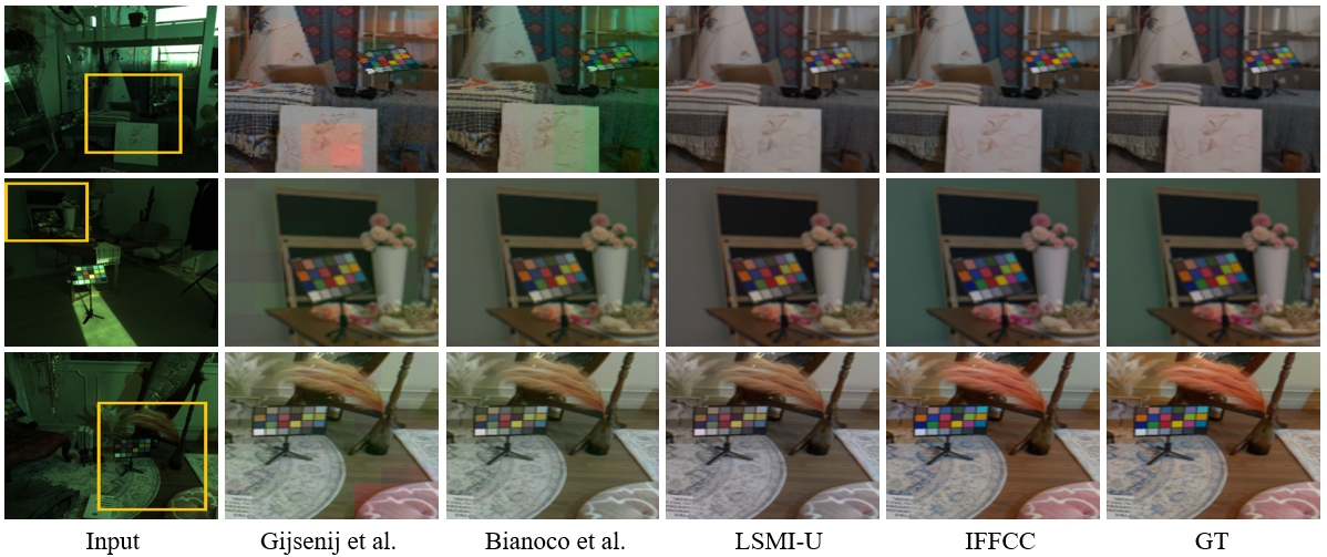
Figure 3: Visualization of the comparison results on the LSMI dataset. For IFFCC, the window size is set to 128 with an overlap of 64. In other patch-based methods, the window size is set to the default value of 32.

Figure 4: Visualization of illumination comparison for different patch-based methods. The window size is 32, with an overlap size of 16.

4.2 Results and Comparisons

Quantitative Comparison We evaluated IFFCC against three traditional methods [29, 4, 24] and three learning-based methods [7, 44, 12] on the Shadow dataset. The experimental results are presented in Tables 1 and 2. Table 1 organizes the Shadow dataset into subsets based on images captured by different cameras, while Table 2 categorizes the dataset by various scene types, each containing photos taken with five distinct cameras. Despite comparisons with advanced network-based methods, IFFCC achieves state-of-the-art performance.

The results in Table 2 highlight the strong generalization ability of IFFCC. Network-based methods generally perform worse than IFFCC on multi-camera datasets, where each camera’s unique spectral sensitivities complicate learning a single mapping across different devices. IFFCC generalizes well across multiple cameras because it leverages an integral log-chroma histogram approach, which directly models chromaticity distributions without being overly reliant on the specific spectral sensitivities of individual cameras. This histogram-based method effectively captures illumination variations across different scenes and cameras, allowing IFFCC to produce robust predictions without requiring extensive fine-tuning for each camera’s unique spectral characteristics.

The experimental results on the LSMI dataset, presented in Tables 3, and 4, provide a comparative analysis of patch-based and pixel-level methods. The test set is categorized into Multi (multiple light sources), and Mixed (comprising both single and multiple light sources). Among patch-based approaches, IFFCC demonstrates state-of-the-art performance, achieving results comparable to those of leading pixel-level methods, including AID [32]. Notably, IFFCC’s compact parameter count and rapid processing speed render it highly suitable for deployment on mobile and resource-constrained devices.

We also compared the processing time for a 256×256 image in a multi-illuminant scene using FFCC and IFFCC, as shown in Table 5. As the number of windows increases, IFFCC significantly outperforms FFCC in processing speed.

Qualitative Comparison Fig.3 visually compares our method against alternative approaches on the LSMI dataset. To enhance visualization quality, color correction, gamma correction, and tone mapping were applied to the white-balanced images. The results indicate that IFFCC achieves more accurate white balance restoration than competing methods. We also present a comparison of illumination maps between our method and patch-based approaches, as shown in Fig.4. The window size is set to $32\times 32$ with an overlap of 16. The results demonstrate that IFFCC achieves a more precise and smoother illumination prediction.

Method		Multi						Params (M)	Time (s)
		Galaxy		Nikon		Sony
		mean	med.	mean	med.	mean	med.
Patch -level	Gijsenij[23]	12.38	9.57	9.31	6.59	11.19	8.14	-	1.3
	Bianoco[7]	5.56	4.34	4.65	4.19	4.38	3.94	0.16	-
	IFFCC	2.48	1.90	2.30	1.50	2.48	1.97	0.012	0.03
Pixel -level	Pix2Pix[30]	4.28	2.63	4.18	2.76	4.37	3.26	5.4	0.48
	LSMI-H[31]	3.13	2.70	3.20	3.01	3.65	3.33	0.52	0.28
	LSMI-U[31]	2.85	2.55	2.36	1.84	2.76	2.38	5.7	0.51
	AID[32]	2.03	1.43	2.26	1.39	2.16	1.64	6.4	$>$1

Table 3: The performance results on the multi-illumination images from the LSMI dataset are presented, with testing time corresponding to the processing time for 256×256 images on a CPU.

Method		Mixed						Params (M)	Time (s)
		Galaxy		Nikon		Sony
		mean	med.	mean	med.	mean	med.
Patch -level	Gijsenij[23]	10.09	7.43	9.21	5.83	9.46	7.13	-	1.3
	Bianoco[7]	4.89	3.83	3.93	3.48	3.84	3.21	0.16	-
	IFFCC	1.98	1.79	2.11	1.48	1.93	1.72	0.012	0.03
Pixel -level	Pix2Pix[30]	5.66	2.44	5.41	2.49	4.20	2.20	5.4	0.48
	LSMI-H[31]	3.06	2.54	2.92	2.63	3.21	2.85	0.52	0.28
	LSMI-U[31]	2.63	1.91	2.16	1.55	2.68	2.29	5.7	0.51
	AID[32]	1.63	1.32	1.76	1.14	1.68	1.44	6.4	$>$1

Table 4: The performance results on the mixed-illumination images (containing both single and multiple light sources) from the LSMI dataset are presented, with testing time corresponding to the processing time for 256×256 images on a CPU.

	[32,0]	[32,16]	[64,32]	[64,48]	[128,64]	[128,96]
FFCC	162ms	450ms	203ms	689ms	88ms	234ms
IFFCC	34ms	46ms	29ms	40ms	27ms	33ms

Table 5: Comparison of average testing time for FFCC and IFFCC on the Shadow dataset, evaluated across different window and overlap sizes. FFCC employs a conventional histogram computation approach.

4.3 Ablation Study

Table 6 presents results from ablation experiments analyzing the impact of various training strategies, window sizes, and overlap regions. Here, “B” represents training with a blend of illumination maps as the ground truth (GT), and “M” uses the dominant light source as GT. Parameters “ws” and “os” indicate window and overlap sizes, respectively. Findings reveal that smaller window sizes, with limited information, reduce prediction accuracy. However, the blended illumination strategy provides improved accuracy compared to using a single dominant light source. Visual comparisons (Fig. 5) show that smaller windows enhance texture details in the predicted illumination maps but with lower accuracy. Conversely, larger windows (e.g., [192, 128]) reduce error metrics by capturing more information, yet they may blur boundaries in multi-illuminant regions, compromising edge clarity.

type	[ws, os]	mean	median	b25	w25
B	[32, 16]	2.65	2.17	1.37	4.65
B	[64, 0]	2.35	2.01	1.13	4.31
M	[64, 32]	2.53	2.04	1.25	4.83
B	[64, 32]	2.37	1.87	1.16	4.38
M	[128, 0]	2.46	2.03	1.04	4.78
B	[128, 0]	2.16	1.68	0.91	4.23
M	[128, 32]	2.50	1.88	1.04	4.91
B	[128, 32]	2.14	1.64	0.85	4.30
M	[128, 64]	2.42	1.95	0.93	4.71
B	[128, 64]	2.06	1.54	0.81	4.19
B	[128, 96]	2.13	1.59	0.83	4.25
B	[192, 128]	1.98	1.34	0.72	4.08

Table 6: Ablation study on the Shadow dataset (Canon5d), reporting the impact of different window sizes, overlap sizes, and training strategies on accuracy.

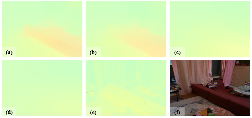
Figure 5: (a)-(d) show illumination maps generated with different window sizes ([32, 16], [64, 32], [128, 64], [192, 128]), each processed with smooth transition adjustments. (e) presents the ground truth (GT) illumination map, and (f) displays the white-balanced image obtained by combining the input image with the GT.

5 Conclusion

We propose IFFCC, a practical solution for achieving accurate, real-time auto white balance (AWB) in multi-illuminant environments. Built upon the Fast Fourier Color Constancy (FFCC) algorithm, IFFCC leverages an integral UV histogram and parallelized Fourier-based convolution to rapidly estimate illumination across different image regions, addressing the need for localized, adaptive AWB. Results on multiple datasets demonstrate that IFFCC delivers accuracy comparable to or surpassing pixel-level neural network methods, while reducing the parameter count by over 400 times and speeding up processing by a factor of 20–100. These advantages make IFFCC highly suitable for resource-limited, real-time applications such as video streaming.

We believe that FFCC-based methods, including IFFCC, will continue to enrich the field and attract increased attention across a broader range of ISP applications.

References

- Barnard et al. [2002] Kobus Barnard, Vlad Cardei, and Brian Funt. A comparison of computational color constancy algorithms. i: Methodology and experiments with synthesized data. IEEE transactions on Image Processing, 11(9):972–984, 2002.
- Barron [2015] Jonathan T Barron. Convolutional color constancy. In Proceedings of the IEEE International Conference on Computer Vision, pages 379–387, 2015.
- Barron and Tsai [2017] Jonathan T Barron and Yun-Ta Tsai. Fast fourier color constancy. In Proceedings of the IEEE conference on computer vision and pattern recognition, pages 886–894, 2017.
- Beigpour et al. [2013] Shida Beigpour, Christian Riess, Joost Van De Weijer, and Elli Angelopoulou. Multi-illuminant estimation with conditional random fields. IEEE Transactions on Image Processing, 23(1):83–96, 2013.
- Bianco and Schettini [2014] Simone Bianco and Raimondo Schettini. Adaptive color constancy using faces. IEEE transactions on pattern analysis and machine intelligence, 36(8):1505–1518, 2014.
- Bianco et al. [2015] Simone Bianco, Claudio Cusano, and Raimondo Schettini. Color constancy using cnns. In Proceedings of the IEEE conference on computer vision and pattern recognition workshops, pages 81–89, 2015.
- Bianco et al. [2017] Simone Bianco, Claudio Cusano, and Raimondo Schettini. Single and multiple illuminant estimation using convolutional neural networks. IEEE Transactions on Image Processing, 26(9):4347–4362, 2017.
- Bleier et al. [2011] Michael Bleier, Christian Riess, Shida Beigpour, Eva Eibenberger, Elli Angelopoulou, Tobias Tröger, and André Kaup. Color constancy and non-uniform illumination: Can existing algorithms work? In 2011 IEEE international conference on computer vision workshops (ICCV Workshops), pages 774–781. IEEE, 2011.
- Buchsbaum [1980a] Gershon Buchsbaum. A spatial processor model for object colour perception. Journal of the Franklin institute, 310(1):1–26, 1980a.
- Buchsbaum [1980b] Gershon Buchsbaum. A spatial processor model for object colour perception. Journal of the Franklin institute, 310(1):1–26, 1980b.
- Cheng et al. [2014] Dongliang Cheng, Dilip K Prasad, and Michael S Brown. Illuminant estimation for color constancy: why spatial-domain methods work and the role of the color distribution. JOSA A, 31(5):1049–1058, 2014.
- Domislović et al. [2021] Ilija Domislović, Donik Vrsnak, Marko Subašić, and Sven Lončarić. Outdoor daytime multi-illuminant color constancy. In 2021 12th International Symposium on Image and Signal Processing and Analysis (ISPA), pages 270–275. IEEE, 2021.
- Domislović et al. [2023a] Ilija Domislović, Donik Vršnak, Marko Subašić, and Sven Lončarić. Shadows & lumination: Two-illuminant multiple cameras color constancy dataset. Expert systems with applications, 224:120045, 2023a.
- Domislović et al. [2023b] Ilija Domislović, Donik Vršnjak, Marko Subašić, and Sven Lončarić. Color constancy for non-uniform illumination estimation with variable number of illuminants. Neural Computing and Applications, 35(20):14825–14835, 2023b.
- Finlayson and Hordley [2001] Graham D Finlayson and Steven D Hordley. Color constancy at a pixel. JOSA A, 18(2):253–264, 2001.
- Finlayson and Trezzi [2004] Graham D Finlayson and Elisabetta Trezzi. Shades of gray and colour constancy. In Color and Imaging Conference, pages 37–41. Society of Imaging Science and Technology, 2004.
- Finlayson et al. [2001] Graham D. Finlayson, Steven D. Hordley, and Paul M. Hubel. Color by correlation: A simple, unifying framework for color constancy. IEEE Transactions on Pattern Analysis and Machine Intelligence, 23(11):1209–1221, 2001.
- Forsyth [1990] David A Forsyth. A novel algorithm for color constancy. International Journal of Computer Vision, 5(1):5–35, 1990.
- Foster [2011] David H Foster. Color constancy. Vision research, 51(7):674–700, 2011.
- Gao et al. [2014] Shaobing Gao, Wangwang Han, Kaifu Yang, Chaoyi Li, and Yongjie Li. Efficient color constancy with local surface reflectance statistics. In Computer Vision–ECCV 2014: 13th European Conference, Zurich, Switzerland, September 6-12, 2014, Proceedings, Part II 13, pages 158–173. Springer, 2014.
- Gijsenij et al. [2010] Arjan Gijsenij, Theo Gevers, and Joost Van De Weijer. Generalized gamut mapping using image derivative structures for color constancy. International Journal of Computer Vision, 86:127–139, 2010.
- Gijsenij et al. [2011a] Arjan Gijsenij, Theo Gevers, and Joost Van De Weijer. Computational color constancy: Survey and experiments. IEEE transactions on image processing, 20(9):2475–2489, 2011a.
- Gijsenij et al. [2011b] Arjan Gijsenij, Theo Gevers, and Joost Van De Weijer. Improving color constancy by photometric edge weighting. IEEE Transactions on Pattern Analysis and Machine Intelligence, 34(5):918–929, 2011b.
- Gijsenij et al. [2011c] Arjan Gijsenij, Rui Lu, and Theo Gevers. Color constancy for multiple light sources. IEEE Transactions on image processing, 21(2):697–707, 2011c.
- He et al. [2012] Kaiming He, Jian Sun, and Xiaoou Tang. Guided image filtering. IEEE transactions on pattern analysis and machine intelligence, 35(6):1397–1409, 2012.
- Hsu et al. [2008] Eugene Hsu, Tom Mertens, Sylvain Paris, Shai Avidan, and Frédo Durand. Light mixture estimation for spatially varying white balance. In ACM SIGGRAPH 2008 papers, pages 1–7. 2008.
- Hu et al. [2017] Yuanming Hu, Baoyuan Wang, and Stephen Lin. Fc4: Fully convolutional color constancy with confidence-weighted pooling. In Proceedings of the IEEE conference on computer vision and pattern recognition, pages 4085–4094, 2017.
- Hui et al. [2016] Zhuo Hui, Aswin C Sankaranarayanan, Kalyan Sunkavalli, and Sunil Hadap. White balance under mixed illumination using flash photography. In 2016 IEEE International Conference on Computational Photography (ICCP), pages 1–10. IEEE, 2016.
- Hussain and Akbari [2018] Md Akmol Hussain and Akbar Sheikh Akbari. Color constancy algorithm for mixed-illuminant scene images. IEEE Access, 6:8964–8976, 2018.
- Isola et al. [2017] Phillip Isola, Jun-Yan Zhu, Tinghui Zhou, and Alexei A Efros. Image-to-image translation with conditional adversarial networks. In Proceedings of the IEEE conference on computer vision and pattern recognition, pages 1125–1134, 2017.
- Kim et al. [2021] Dongyoung Kim, Jinwoo Kim, Seonghyeon Nam, Dongwoo Lee, Yeonkyung Lee, Nahyup Kang, Hyong-Euk Lee, ByungIn Yoo, Jae-Joon Han, and Seon Joo Kim. Large scale multi-illuminant (lsmi) dataset for developing white balance algorithm under mixed illumination. In Proceedings of the IEEE/CVF International Conference on Computer Vision, pages 2410–2419, 2021.
- Kim et al. [2024] Dongyoung Kim, Jinwoo Kim, Junsang Yu, and Seon Joo Kim. Attentive illumination decomposition model for multi-illuminant white balancing. In Proceedings of the IEEE/CVF Conference on Computer Vision and Pattern Recognition, pages 25512–25521, 2024.
- Land [1974] Edwin H Land. The retinex theory of color vision. In Proceedings of the Royal Institution of Great Britain, page 23, 1974.
- Li et al. [2022] Shuwei Li, Jikai Wang, Michael S Brown, and Robby T Tan. Transcc: Transformer-based multiple illuminant color constancy using multitask learning. arXiv preprint arXiv:2211.08772, 1(2):3, 2022.
- Liu and Shen [2019] Yongjie Liu and Sijie Shen. Self-adaptive single and multi-illuminant estimation framework based on deep learning. arXiv preprint arXiv:1902.04705, 2019.
- Lo et al. [2021] Yi-Chen Lo, Chia-Che Chang, Hsuan-Chao Chiu, Yu-Hao Huang, Chia-Ping Chen, Yu-Lin Chang, and Kevin Jou. Clcc: Contrastive learning for color constancy. In Proceedings of the IEEE/CVF Conference on Computer Vision and Pattern Recognition, pages 8053–8063, 2021.
- Locatello et al. [2020] Francesco Locatello, Dirk Weissenborn, Thomas Unterthiner, Aravindh Mahendran, Georg Heigold, Jakob Uszkoreit, Alexey Dosovitskiy, and Thomas Kipf. Object-centric learning with slot attention. Advances in neural information processing systems, 33:11525–11538, 2020.
- Mardia [1975] Kantilal Varichand Mardia. Statistics of directional data. Journal of the Royal Statistical Society Series B: Statistical Methodology, 37(3):349–371, 1975.
- Murmann et al. [2019] Lukas Murmann, Michael Gharbi, Miika Aittala, and Fredo Durand. A dataset of multi-illumination images in the wild. In Proceedings of the IEEE/CVF International Conference on Computer Vision, pages 4080–4089, 2019.
- Porikli [2005] Fatih Porikli. Integral histogram: A fast way to extract histograms in cartesian spaces. In 2005 IEEE Computer Society Conference on Computer Vision and Pattern Recognition (CVPR’05), pages 829–836. IEEE, 2005.
- Qian et al. [2017] Yanlin Qian, Ke Chen, Jarno Nikkanen, Joni-Kristian Kamarainen, and Jiri Matas. Recurrent color constancy. In Proceedings of the IEEE international conference on computer vision, pages 5458–5466, 2017.
- Qian et al. [2019] Yanlin Qian, Joni-Kristian Kamarainen, Jarno Nikkanen, and Jiri Matas. On finding gray pixels. In CVPR, 2019.
- Qian et al. [2020] Yanlin Qian, Jani Käpylä, Joni-Kristian Kämäräinen, Samu Koskinen, and Jiri Matas. A benchmark for burst color constancy. In ECCVW, 2020.
- Shi et al. [2016] Wu Shi, Chen Change Loy, and Xiaoou Tang. Deep specialized network for illuminant estimation. In Computer Vision–ECCV 2016: 14th European Conference, Amsterdam, The Netherlands, October 11–14, 2016, Proceedings, Part IV 14, pages 371–387. Springer, 2016.
- Sidorov [2019a] Oleksii Sidorov. Conditional gans for multi-illuminant color constancy: Revolution or yet another approach? In Proceedings of the IEEE/CVF conference on computer vision and pattern recognition workshops, pages 0–0, 2019a.
- Sidorov [2019b] Oleksii Sidorov. Conditional gans for multi-illuminant color constancy: Revolution or yet another approach? In Proceedings of the IEEE/CVF conference on computer vision and pattern recognition workshops, pages 0–0, 2019b.
- Van De Weijer et al. [2007] Joost Van De Weijer, Theo Gevers, and Arjan Gijsenij. Edge-based color constancy. IEEE Transactions on image processing, 16(9):2207–2214, 2007.
- Xu et al. [2020] Bolei Xu, Jingxin Liu, Xianxu Hou, Bozhi Liu, and Guoping Qiu. End-to-end illuminant estimation based on deep metric learning. In Proceedings of the IEEE/CVF Conference on Computer Vision and Pattern Recognition, pages 3616–3625, 2020.