LanPaint: Training-Free Diffusion Inpainting with Fast and Exact Conditional Inference

Abstract

Diffusion models generate high-quality images but often lack efficient and universally applicable inpainting capabilities, particularly in community-trained models. We introduce LanPaint, a training-free method tailored for widely adopted ODE-based samplers, which leverages Langevin dynamics to perform exact conditional inference, enabling precise and visually coherent inpainting. LanPaint addresses two key challenges in Langevin-based inpainting: (1) the risk of local likelihood maxima trapping and (2) slow convergence. By proposing a guided score function and a fast-converging Langevin framework, LanPaint achieves high-fidelity results in very few iterations. Experiments demonstrate that LanPaint outperforms existing training-free inpainting techniques, outperforming in challenging tasks such as outpainting with Stable Diffusion.

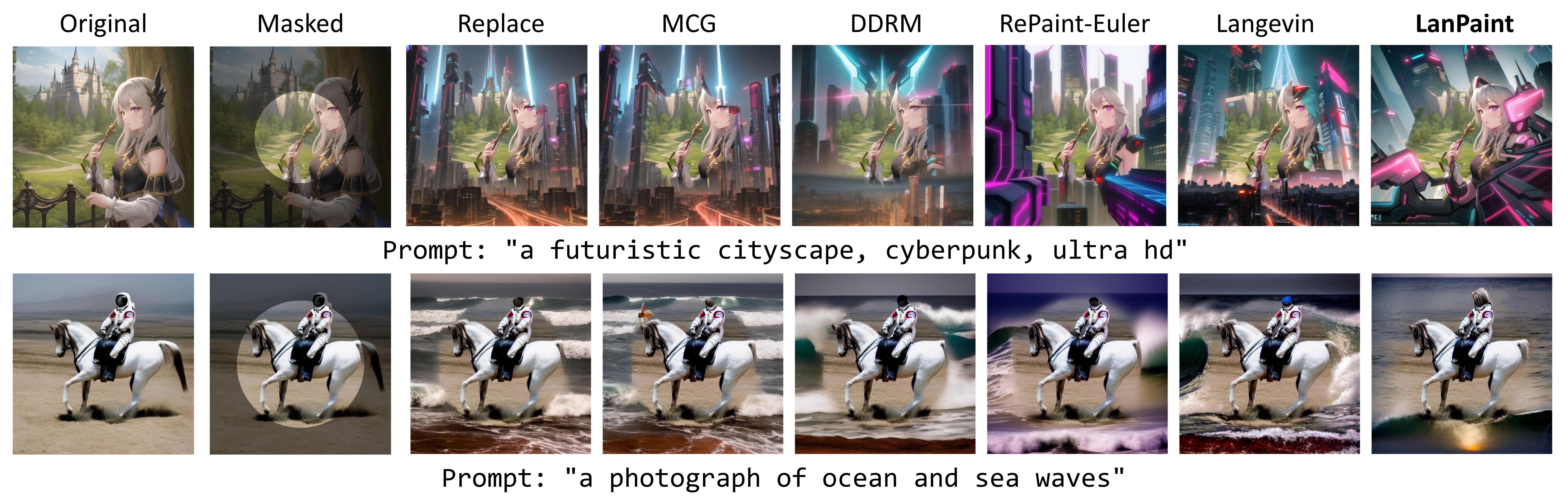
Figure 1: Qualitative comparison of circle-masked out-painting on Anything V5 (Yuno779, 2023) and Stable Diffusion v1.4 (Rombach et al., 2021) using an Euler Discrete sampler (Karras et al., 2022) (20 steps). Each row presents the masked image (left), then outputs from Replace, MCG, DDRM, RePaint, Langevin, and LanPaint (from left to right). RePaint, Langevin, and LanPaint each use 5 inner iterations. To make the task more challenging, the prompt that significantly deviate from the original image content, such as “a futuristic cityscape” guide the inpainting. LanPaint achieves visually coherent and contextually relevant completions.

1 Introduction

Diffusion models (Sohl-Dickstein et al., 2015; Song & Ermon, 2019a; Song et al., 2020b) have emerged as powerful generative frameworks that produce high-quality outputs through iterative denoising. The Denoising Diffusion Probabilistic Model (DDPM) (Ho et al., 2020) has become a cornerstone of this field, enabling state-of-the-art text-to-image systems like Stable Diffusion (Rombach et al., 2021) and DALL·E (Betker et al., 2023). Subsequent advances in ODE-based samplers (Karras et al., 2022; Lu et al., 2022; Zhao et al., 2023) have dramatically improved efficiency, reducing sampling steps from hundreds to dozens. These innovations, combined with community-trained model variants, have broadened the scope and quality of generative visual content.

Despite these advancements, a critical challenge remains: how to edit or refine generated images when the initial output does not meet user expectations. Inpainting—filling in missing or undesired regions of an image—is a common solution, but many community-trained diffusion models (i.e (Park et al., 2024)) lack robust inpainting capabilities. Existing approaches (Xie et al., 2023; Corneanu et al., 2024) often require additional training, are computationally expensive, or produce artifacts and discontinuities in the edited regions. As a result, there is a pressing need for a training-free, fast, and accurate inpainting solution that is widely applicable to existing pre-trained diffusion models with high visual fidelity.

Training-free inpainting tackles the challenge of sampling from conditional distributions (e.g., given partial observations) when the underlying DDPM is designed for joint distribution modeling. Existing methods, such as RePaint’s “time travel” technique (Lugmayr et al., 2022), Sequential Monte Carlo (Cardoso et al., 2023; Trippe et al., 2022), and Langevin dynamics (Janati et al., 2024; Cornwall et al., 2024), often require hundreds of sampling steps with dozens of inner iterations, resulting in high computational costs. Additionally, these methods are designed for DDPM sampling without considering ODE-based samplers, often requiring non-trivial adaptations or introducing new challenges. Techniques such as DPS (Chung et al., 2022a), Manifold Constrained Gradient (Chung et al., 2022b), GradPaint (Grechka et al., 2024), and DDRM (Kawar et al., 2022) are faster. However, these methods are not exact; they rely on heuristics (e.g., image smoothness) or simplifying assumptions that compromise accuracy. As a result, their applicability to general data types is limited, and their performance is often constrained.

In this work, we propose LanPaint, a training-free and efficient inpainting method based on Langevin dynamics, tailored for ODE-based samplers. LanPaint achieves theoretically exact conditional sampling (given partial observations) without requiring data-specific assumptions. It introduces two core innovations: (1) Bidirectional Guided (BiG) Score, which enables mutual adaptation between inpainted and observed regions, avoids local maxima traps caused by ODE-samplers with large diffusion steps. This significantly improves in-painting quality; and (2) Fast Langevin Dynamics (FLD), an accelerated sampling framework that achieves high-fidelity results in just 5 inner iterations per step—drastically reducing computational costs compared to prior training-free methods requiring tens of iterations. Experiments confirm that LanPaint outperforms existing approaches, delivering high-quality inpainting and outpainting results for both pixel-space and latent-space models.

2 Related Works

2.1 Diffusion Models

Diffusion models, particularly DDPMs (Ho et al., 2020), generate high-quality samples through iterative corruption and denoising (Anderson, 1982a). However, DDPMs inherently model the joint distribution of pixels, making it challenging to preserve known regions of pixels while generating the remaining parts. This limitation complicates tasks like inpainting, where partial observations must remain fixed during sampling.

Recent advances like bridge models (Liu et al., 2022b, 2023; Zhou et al., 2023) shed new light on conditional generation by rethinking the diffusion process. While promising, these methods redesign the framework, limiting compatibility with existing large-scale pretrained diffusion models. In contrast, our work aims to incorporate conditioning without altering the core diffusion model architecture, ensuring seamless compatibility with powerful pretrained models.

2.2 ODE-based Sampling Methods

Vanilla DDPMs are slow, often requiring hundreds of denoising steps. To address this, acceleration strategies have emerged, such as approximate diffusion processes (Song et al., 2020b; Liu et al., 2022a; Song et al., 2020a; Zhao et al., 2023) and advanced ODE solvers (Karras et al., 2022; Lu et al., 2022; Zhao et al., 2023). These methods convert stochastic DDPM sampling into deterministic ODE flows, enabling larger time steps and faster generation. However, this shift breaks the probabilistic foundations of inpainting techniques like Sequential Monte Carlo (Cardoso et al., 2023; Trippe et al., 2022) and Bayesian posterior analysis (Janati et al., 2024), making their adaptation to ODE frameworks non-trivial.

In this work, we propose a fast conditional inference framework that is fully compatible with accelerated sampling methods, enabling efficient and high-quality conditional generation.

2.3 Conditional Inference with Diffusion Models

While DDPMs have achieved significant success, they lack inherent support for conditional sampling with partial observations. RePaint (Lugmayr et al., 2022) addresses this via a “time travel” mechanism, but typical configurations (e.g., RePaint-20 with 250 denoising steps and 20 inner iterations per step) are computationally expensive. Moreover, its reliance on a complex time “jump” schedule—designed for DDPMs—limits compatibility with fast samplers (FBehrad, 2022).

Recent work has reinterpreted RePaint’s “time travel” mechanism as a form of Monte Carlo sampling using Langevin dynamics (Janati et al., 2024; Cornwall et al., 2024). Building on this insight, methods like DCPS (Janati et al., 2024) combine Langevin dynamics with Diffusion Probabilistic Sampling (DPS) for inpainting, but remain tailored to DDPMs and are non-trivial to adapt to fast samplers. Concurrent with our work, studies (Cornwall et al., 2024) demonstrate that Langevin-based approaches achieve better convergence than RePaint, yet they still focus on DDPMs and neglect ODE-based solvers. We observed that Langevin methods have decoupled RePaint’s time ‘travel’ from diffusion sampling, hence can enable better compatibility with ODE samplers—an advantage we will leverage.

Alternative approaches, such as Sequential Monte Carlo (SMC) (Cardoso et al., 2023; Trippe et al., 2022; Wu et al., 2024), enable exact conditional sampling but require hundreds of steps and large particle sets, resulting in significant computational overhead. Additionally, their reliance on DDPM’s probabilistic interpretation makes adaptation to fast ODE solvers highly non-trivial.

Beyond Monte Carlo methods, which prioritize exact conditional sampling, faster alternatives like Blended Latent Diffusion (Avrahami et al., 2023), variational inference (e.g., DDRM (Kawar et al., 2022)), and heuristic strategies (e.g., DPS (Chung et al., 2022a), Manifold Constrained Gradient (Chung et al., 2022b), GradPaint (Grechka et al., 2024)) achieve accelerated inpainting. However, these approaches rely on approximations or data-specific heuristics, limiting their accuracy and generalizability across diverse data types. In this work, we bridge this gap by proposing a fast, training-free Monte Carlo method that retains exactness while enabling efficient inpainting and general conditional inference.

3 Background

3.1 DDPM and Fast Sampling

DDPMs learn a target distribution $p(\mathbf{z})$ by reconstructing a clean data point $\mathbf{z}_{0}\sim p(\mathbf{z})$ from progressively noisier versions. The forward diffusion process gradually contaminates $\mathbf{z}_{0}$ with Gaussian noise. A discrete-time formulation of this process is:

$$\mathbf{z}_{i}=\sqrt{\bar{\alpha}_{t_{i}}}\,\mathbf{z}_{0}+\sqrt{1-\bar{\alpha}_{t_{i}}}\,\bar{\boldsymbol{\epsilon}}_{i},\quad 1\leq i\leq n,$$ (1)

where $\bar{\boldsymbol{\epsilon}}_{i}\sim\mathcal{N}(\mathbf{0},\mathbf{I})$ is Gaussian noise. This arises from discretizing the continuous-time Ornstein–Uhlenbeck (OU) process:

$$d\mathbf{z}_{t}=-\tfrac{1}{2}\,\mathbf{z}_{t}\,dt\;+\;d\mathbf{W},$$ (2)

where $\bar{\alpha}_{t}=e^{-t}$ and $d\mathbf{W}$ is a Brownian motion increment. The OU process ensures $\mathbf{z}_{t}$ transitions smoothly from the data distribution $p(\mathbf{z})$ to pure noise $\mathcal{N}(\mathbf{0},\mathbf{I})$.

To sample from $p(\mathbf{z})$, we reverse the diffusion process. Starting from noise $\mathbf{z}_{T}\sim\mathcal{N}(\mathbf{0},\mathbf{I})$, the reverse-time SDE (Anderson, 1982b) is:

$$d\mathbf{z}_{t^{\prime}}=\Bigl{(}\tfrac{1}{2}\,\mathbf{z}_{t^{\prime}}+\mathbf{s}(\mathbf{z},\,T-t^{\prime})\Bigr{)}\,dt^{\prime}+d\mathbf{W},$$ (3)

where $t^{\prime}\in[0,\,T]$ is the backward time, $t=T-t^{\prime}$, and $\mathbf{s}(\mathbf{z},t)=\nabla_{\mathbf{z}}\log p(\mathbf{z}_{t})$ is the score function, which guides noise removal. The score function is usually learnt as a denoising neural network, see Appendix.A.

Replacing the stochastic term in (3) with a deterministic drift yields an ODE-based sampler:

$$d\mathbf{z}_{t^{\prime}}=\tfrac{1}{2}\Bigl{(}\mathbf{z}_{t^{\prime}}+\mathbf{s}(\mathbf{z},\,T-t^{\prime})\Bigr{)}\,dt^{\prime}.$$ (4)

While this allows larger time steps hence faster sampling. However, it poses challenges for inpainting techniques like Sequential Monte Carlo (Cardoso et al., 2023; Trippe et al., 2022), which rely heavily on the probabilistic interpretation of diffusion models, leaving their adaptation to ODE frameworks unresolved.

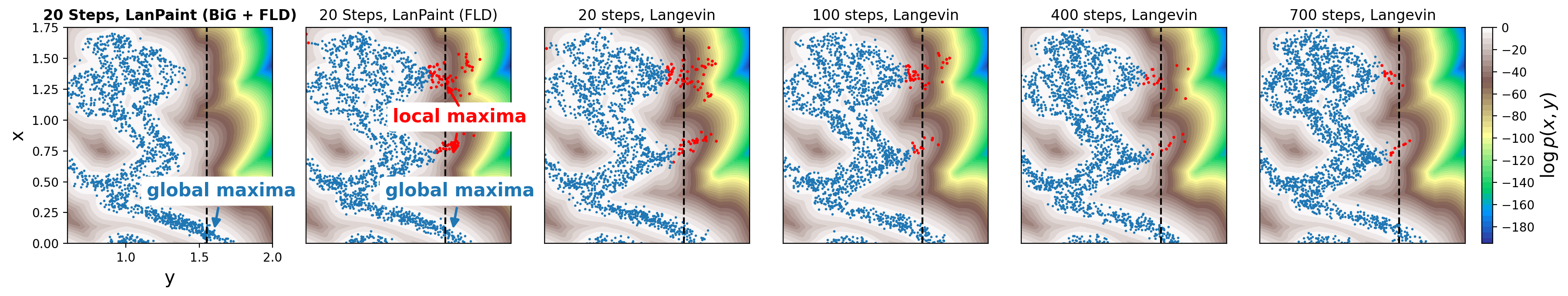
Figure 2: Inpainting $x$ given observed $y$ using ODE-based diffusion sampler (Experiment in Section 5.1). The Euler Discrete scheduler (Karras et al., 2022) governs the diffusion process, while inpainting methods (LanPaint, Langevin) perform 10 inner iterations per diffusion step to refine $x$. Red dots indicate samples with low joint likelihood that should not have appeared, trapped at local maxima of $p(x\mid y=1.55)$ along the dashed line. Reducing total diffusion steps (right to left) increases trapped samples—a key limitation of Langevin/RePaint inpainting with ODE samplers. The left panel demonstrates that LanPaint’s guided Langevin dynamics (BiG score) circumvents these traps, aligning samples with the global maxima of $p(x\mid y)$.

3.2 Conditional Inference

Conditional inference in DDPMs poses a significant challenge due to the inaccessibility of the conditional score function. Specifically, consider a DDPM modeling a joint distribution $p(\mathbf{x},\mathbf{y})$. Conditional sampling aims to generate $\mathbf{x}\sim p(\mathbf{x}\mid\mathbf{y}=\mathbf{y}_{0})$. While the DDPM provides joint scores:

$$\mathbf{s}_{\mathbf{x}}(\mathbf{x},\mathbf{y},t) =\nabla_{\mathbf{x}}\log p(\mathbf{x}_{t},\mathbf{y}_{t}),$$ (5)

$$\mathbf{s}_{\mathbf{y}}(\mathbf{x},\mathbf{y},t) =\nabla_{\mathbf{y}}\log p(\mathbf{x}_{t},\mathbf{y}_{t}),$$ (6)

the conditional score $\nabla_{\mathbf{x}}\log p(\mathbf{x}_{t},\mathbf{y}_{t}\mid\mathbf{y}_{0})$—required for direct sampling from $p(\mathbf{x}_{t}\mid\mathbf{y}_{0})$—is inaccessible. A naive backward process sampling $(\mathbf{x}_{t},\mathbf{y}_{t})\sim p(\mathbf{x}_{t},\mathbf{y}_{t})$ fails to enforce $\mathbf{y}_{t}\to\mathbf{y}_{0}$, necessitating alternative approaches.

Decoupling Approximation One could assume the conditioned joint distribution $p(\mathbf{x}_{t},\mathbf{y}_{t}\mid\mathbf{y}_{0})$ as:

$$p(\mathbf{x}_{t},\mathbf{y}_{t}\mid\mathbf{y}_{0})\approx p(\mathbf{x}_{t}\mid\mathbf{y}_{t})\cdot p(\mathbf{y}_{t}\mid\mathbf{y}_{0}).$$ (7)

Here, $p(\mathbf{y}_{t}\mid\mathbf{y}_{0})=\mathcal{N}\!\bigl{(}\mathbf{y}_{t}\mid\sqrt{\bar{\alpha}_{t}}\mathbf{y}_{0},(1-\bar{\alpha}_{t})\mathbf{I}\bigr{)}$ is derived from the forward process, while $p(\mathbf{x}_{t}\mid\mathbf{y}_{t})$ uses the joint score $\mathbf{s}_{\mathbf{x}}$. Although this decoupling introduces dependencies between $\mathbf{x}_{t}$ and $\mathbf{y}_{t}$ (unlike the original DDPM framework where $\mathbf{x}_{t}$ and $\mathbf{y}_{t}$ are independent given $\mathbf{y}_{0}$), it is tractable and empirically effective.

The Replace Method (Song & Ermon, 2019b) approximates (7) by replacing $\mathbf{y}_{t}$ in each backward iteration with

$$\mathbf{y}_{t}\sim p(\mathbf{y}_{t}\mid\mathbf{y}_{0}),$$ (8)

while diffuse $\mathbf{x}_{t}$ using the unconditional scores in (5). This mix yields sequences

$$(\mathbf{x}_{t},\mathbf{y}_{t})\sim\text{Between}\,[\,p(\mathbf{x}_{t},\mathbf{y}_{t})\,]\;\text{and}\;[\,p(\mathbf{x}_{t}\mid\mathbf{y}_{t})\,p(\mathbf{y}_{t}\mid\mathbf{y}_{0})\,].$$ (9)

While straightforward, this method can be inaccurate. In inpainting tasks, for example, it may create sharp boundaries between the conditioned and unconditioned regions (Lugmayr et al., 2022).

RePaint (Lugmayr et al., 2022) improves over the Replace Method by introducing a “time traveling” step that refines $\mathbf{x}_{t}$. At each diffusion step $t_{i}$, it performs multiple inner iterations, alternating between forward and backward moves:

$$\mathbf{x}_{t_{i}}^{(k+1)}=\underbrace{\mbox{Forward}_{t_{i-n}\to t_{i}}}_{\text{via \eqref{eq:OU_process_noise}}}\;\circ\;\underbrace{\mbox{Backward}_{t_{i}\to t_{i-n}}}_{\text{via \eqref{eq:reverse_diffusion_sde}}}(\mathbf{x}_{t_{i}}^{(k)}).$$ (10)

Where $n$ is the jump steps. Meanwhile, $\mathbf{y}_{t}$ is still replaced at each step by (8). By adding (2) and (3) over the same time increment $d\tau=t_{i}-t_{i-n}$, RePaint effectively simulates the Langevin dynamics (see (13)):

$$d\mathbf{x}_{t_{i}}=\mathbf{s}_{\mathbf{x}}(\mathbf{x}_{t_{i}},\mathbf{y}_{t_{i}},t_{i})\,d\tau+\sqrt{2}\,d\mathbf{W},$$ (11)

whose stationary distribution is $p(\mathbf{x}_{t_{i}}\mid\mathbf{y}_{t_{i}})$. After sufficient iterations, RePaint produces the sequence (7)

$$\mathbf{x}_{t},\mathbf{y}_{t}\sim p(\mathbf{x}_{t}|\mathbf{y}_{t})p(\mathbf{y}_{t}|\mathbf{y}_{0}).$$ (12)

While RePaint was originally designed for DDPMs (which rely on SDE-based backward steps), we successfully adapt it to ODE-based Euler Discrete samplers (Karras et al., 2022) by replacing the backward SDE in (3) with a backward Euler sampling step and set $n=1$, see Appendix D. We call this adaptation Repaint-Euler.

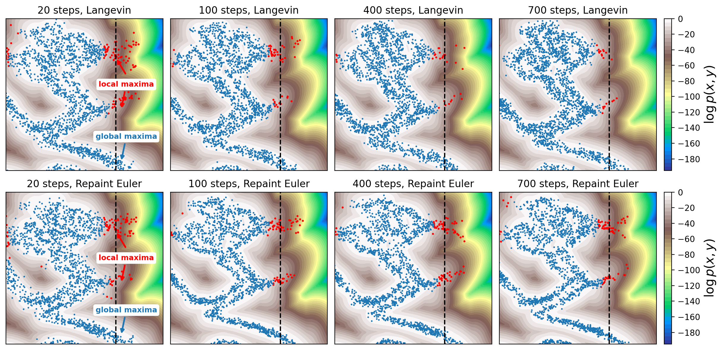
Figure 6: Local maxima trapping in RePaint vs. Langevin-based inpainting (Experiment 5.1): Inpainting $x$ given $y$ using fast diffusion samplers governed by the Euler scheduler. Both methods refine $x$ with 10 inner iterations per Euler step. Red dots denote samples trapped at local maxima of $p(x\mid y)$. Langevin reduces trapping as sampling steps increase, while RePaint remains trapped regardless. This arises because RePaint’s iteration step size is coupled to sampling steps: increasing total steps shrinks per-iteration step size, rendering it insensitive to sample count.

However, RePaint still has three notable drawbacks in practice: (1) The step size $d\tau$ must strictly align with the backward diffusion step $dt$, limiting stability under aggressive step sizes for accelerated sampling; (2) Samples $\mathbf{x}$ is susceptible to trapping in local maxima of $p(\mathbf{x}_{t}\mid\mathbf{y}_{t})$ (Fig.6); (3) It requires many computationally expensive inner-loop iterations (about 20) per diffusion step, hindering efficiency.

Langevin Dynamics Methods

are Monte Carlo sampling techniques that simulate the dynamics of (11) without relying on the diffusion process’s step schedule. For a target distribution $p(\mathbf{z})$, the Langevin stochastic differential equation (SDE):

$$d\mathbf{z}=\mathbf{s}(\mathbf{z})\,d\tau+\sqrt{2}\,d\mathbf{W},$$ (13)

where $\mathbf{s}(\mathbf{z})=\nabla_{\mathbf{z}}\log p(\mathbf{z})$, asymptotically converges to samples $\mathbf{z}\sim p(\mathbf{z})$ as $\tau\to\infty$. While theoretically sound, this method risks trapping samples at local maxima of $p(\mathbf{z})$.

Recent works (Janati et al., 2024; Cornwall et al., 2024) replace the back-forward moves (10) with the Langevin dynamics (11) as inner iterations, enabling adaptive step size control $d\tau$. Despite improved flexibility, this requires multiple Langevin iterations per diffusion step $t_{i}$. Moreover, as shown in Fig. 2 and Fig. 6, local maxima trapping persists, underscoring unresolved limitations.

4 Methodology

To address limitations in Langevin-based sampling for diffusion models, we propose LanPaint, which introduces two novel enhancements targeting the two core components of Langevin dynamics: (1) the target score function $\mathbf{s}(\mathbf{z})$, and (2) the governing stochastic differential equation (SDE) in (13). Specifically:

• Bidirectional Guided (BiG) Score: We design a bidirectional score function that propagates information between inpainted and known regions, avoiding sampling traps in local maxima.

• Fast Langevin Dynamics (FLD): We reformulate the SDE in (13) to accelerate convergence through momentum and preconditioning, significantly reducing the number of inner-loop iterations per diffusion step.

4.1 Bidirectional Guided (BiG) Score

In RePaint and Langevin-based approaches, the inpainted region $\mathbf{x}_{t_{i}}$ is updated using the observed region $\mathbf{y}_{t_{i}}$ during inner iterations, but $\mathbf{y}_{t_{i}}$ remains independent of $\mathbf{x}_{t_{i}}$. This one-way dependency creates a critical flaw: if $\mathbf{x}_{t_{i}}$ enters a suboptimal region of $p(\mathbf{x}_{t}\mid\mathbf{y}_{t})$, $\mathbf{y}_{t_{i}}$ cannot receive corrective feedback, resulting in local maxima trapping (Fig. 2).

To escape such traps, we propose jointly updating $\mathbf{x}_{t_{i}}$ and $\mathbf{y}_{t_{i}}$, establishing bidirectional feedback:

• $\mathbf{x}_{t_{i}}$ is refined by by $\mathbf{y}_{t_{i}}$ (as in prior methods),

• $\mathbf{y}_{t_{i}}$ is guided by $\mathbf{x}_{t_{i}}$ while preserving its observed contents.

This interdependence prevents trapping: if $\mathbf{x}_{t}$ enters a suboptimal region, $\mathbf{y}_{t}$ dynamically adjusts to guide $\mathbf{x}_{t}$ toward higher-likelihood configurations, avoiding local maxims, as demonstrated in Fig.2.

BIG score. We implement this idea by modifying the Langevin dynamics to update both variables jointly:

$$d\mathbf{x}_{t_{i}} ={\mathbf{s}_{\mathbf{x}}(\mathbf{x}_{t_{i}},\mathbf{y}_{t_{i}},t\bigr{)}}d\tau+\sqrt{2}\,d\mathbf{W}_{\mathbf{x}},$$ (14)

$$d\mathbf{y}_{t_{i}} =\underbrace{\mathbf{g}_{\lambda}\bigl{(}\mathbf{x}_{t_{i}},\mathbf{y}_{t_{i}},t\bigr{)}}_{\text{Adaptive guidance term}}d\tau+\sqrt{2}\,d\mathbf{W}_{\mathbf{y}},$$

where $\mathbf{s}_{\mathbf{x}}$ and $\mathbf{s}_{\mathbf{y}}$ are the partial score functions defined in (5), and $\mathbf{g}_{\lambda}$ combines the observation $\mathbf{y}_{0}$ with the unconditional score $\mathbf{s}_{\mathbf{y}}$:

$$\mathbf{g}_{\lambda}=\Bigl{[}(1+\lambda)\,\underbrace{\frac{\sqrt{\bar{\alpha}_{t_{i}}}\mathbf{y}_{0}-\mathbf{y}_{t_{i}}}{1-\bar{\alpha}_{t_{i}}}}_{\text{Score of }p(\mathbf{y}_{t_{i}}\mid\mathbf{y}_{0})}-\lambda\,\underbrace{\mathbf{s}_{\mathbf{y}}\bigl{(}\mathbf{x}_{t_{i}},\mathbf{y}_{t_{i}},t\bigr{)}}_{\text{Score of }p(\mathbf{y}_{t_{i}}\mid\mathbf{x}_{t_{i}})}\Bigr{]}.$$ (15)

with $\lambda>-1$ as the guidance scale. The intuition behind BiG score is to achieve the following:

• $\lambda=-1$: The BiG score reduces to unconditional sampling.

• $\lambda=0$: The BiG score aligns with RePaint-like inpainting, consistent with (12).

• $\lambda>0$: The BiG score amplifies the inpainting effect on $\mathbf{y}$ by penalizing feedback from $\mathbf{x}$: the unconditional scores $\mathbf{s}_{\mathbf{y}}$.

Larger $\lambda$ gives stronger feedback from $\mathbf{x}_{t_{i}}$, enabling better correction of $\mathbf{y}_{t_{i}}$ to escape local traps.

Though the scale $\lambda$ is introduced, the BiG score still yields exact conditional samples given partial observation, as shown in the following theorem:

Theorem 4.1 (Exact Conditional Sampler).

Under the dynamics (14), the joint state $(\mathbf{x}_{t},\mathbf{y}_{t})$ converges to the distribution

$$\mathbf{x}_{t},\,\mathbf{y}_{t}\;\sim\;\frac{1}{Z}\,p(\mathbf{x}_{t}\mid\mathbf{y}_{t})\,\tfrac{p(\mathbf{y}_{t}\mid\mathbf{y}_{0})^{1+\lambda}}{p(\mathbf{y}_{t})^{\lambda}}+o(\sqrt{1-\bar{\alpha}_{t}}),$$ (16)

where $Z$ is a normalizing constant. Consequently, at $t=0$, the marginal $\mathbf{x}_{0}\sim p(\mathbf{x}_{0}\mid\mathbf{y}_{0})$ is an exact conditional sample. (Proof in Appendix C)

In summary, the BiG score enables bidirectional feedback between $\mathbf{x}_{t_{i}}$ and $\mathbf{y}_{t_{i}}$, avoiding local maxima trapping while preserving the exactness of conditional sampling.

4.2 Fast Langevin Dynamics (FLD)

We propose the Fast Langevin Dynamics (inspired by underdamped Langevin dynamics (Cheng et al., 2018), preconditioning techniques (AlRachid et al., 2018), and the HFHR approach (Li et al., 2022)) that accelerates convergence of Langevin dynamics (13). To simplify notation, let $\mathbf{z}=(\mathbf{x}_{t_{i}},\mathbf{y}_{t_{i}})$. Then FLD is the following system improving (13) with momentum, mixing, and pre-conditioning:

$$d\mathbf{z}\;= \frac{1}{m}\,P\,\mathbf{v}\,d\tau\;+\;\alpha\,P\,\mathbf{s}(\mathbf{z})\,d\tau\;+\;\sqrt{2\,\alpha\,P}\;dW_{\mathbf{z}},$$ (17)

$$d\mathbf{v}\;= -\,\frac{\gamma}{m}\,P\,\mathbf{v}\,d\tau\;+\;P\,\mathbf{s}(\mathbf{z})\,d\tau\;+\;\sqrt{2\,\gamma\,P}\;dW_{\mathbf{v}},$$

where $\mathbf{v}$ is a new momentum variable, $m$ (mass), $\gamma$ (friction), and $\alpha$ (mixing) are positive parameters, and $P$ is a positive-definite pre-conditioning matrix with Cholesky factor $\sqrt{P}$. In practice, we choose

$$\small P\;=\;\begin{pmatrix}\mathbf{I}&\mathbf{0}\\[4.0pt] \mathbf{0}&\beta\,\sqrt{\,1-\bar{\alpha}_{t}\,}\,\mathbf{I}\end{pmatrix},$$ (18)

where $\beta>0$ controls the scaling for $\mathbf{y}$. Additionally, we set the step size $d\tau=\min\{\,\eta\,\sqrt{1-\bar{\alpha}_{t}},\,-\log\bar{\alpha}_{t}/2\,\},$ where $\eta$ is a step-size parameter. FLD is simulated with an ABCBA operator splitting (Strang, 1968), as detailed in Algorithm 1.

To build intuition, observe that Langevin dynamics (13) behaves like an object at position $\mathbf{z}$ moves under force $\mathbf{s}$ as if through extremely viscous fluid (e.g. thick honey), with friction so high that no momentum can build up. FLD admits lower friction $\gamma$ and introduces momentum $\mathbf{v}$, allowing faster movement—like traveling through air instead of honey. Mass $m$ controls inertia, and $P$ defines the body’s shape: $P=I$ means a sphere, whereas other $P$ yield a more streamlined ellipsoid and faster movement. Additionally, $\alpha$ sets a background flow: $\alpha=0$ means the fluid is still, and increasing $\alpha$ strengthens the flow along $\mathbf{s}(\mathbf{z})$, accelerating the object’s movement. By tuning $\gamma$, $m$, $P$, and $\alpha$, FLD significantly speeds up convergence compared to the original Langevin dynamics.

A key property of FLD is that it preserves the stationary distribution of the original Langevin dynamics, as shown in the following theorem.

Theorem 4.2 (Stationary Distribution).

Under the fast Langevin dynamics (17), the joint state $(\mathbf{z},\mathbf{v})$ has a stationary distribution given by

$$(\mathbf{z},\mathbf{v})\;\sim\;p(\mathbf{z})\;\times\;\mathcal{N}(\mathbf{v}\mid\mathbf{0},\,m\,\mathbf{I}).$$

Hence, $\mathbf{z}$ alone retains the same stationary distribution as the original Langevin dynamics (13), so introducing $\mathbf{v}$ speeds up convergence without altering the target distribution. (Proof in Appendix B)

Consequently, FLD accelerates sampling while maintaining the desired stationary distribution. We demonstrate these efficiency gains in subsequent experiments.

5 Experiments

5.1 Mixture of Gaussian

We validate LanPaint on a synthetic mixture-of-Gaussians (MoG) benchmark with analytical ground truth distribution to address two key challenges: escaping local maxima and accelerating convergence. The experiments are structured to (1) compare overall inpainting performance against five baselines, (2) validate the effectiveness of BiG score in avoiding local maxima, (3) the convergence efficiency of FLD, and (4) quantify the contributions of BiG score and FLD. The controlled setting provides exact validation of theoretical improvements of LanPaint.

We evaluate several inpainting methods (Appendix D)—Replace (Song & Ermon, 2019b), MCG (Chung et al., 2022b), DDRM (Kawar et al., 2022), RePaint (Lugmayr et al., 2022), Langevin, and LanPaint—on a synthetic 2D task where masked $x$-coordinates are inferred from observed $y$-values. The target distribution is derived from a Gaussian mixture model (GMM) fitted to a wizard bear silhouette image. Performance is measured via KL divergence between inpainted samples and the ground truth GMM (lower is better). More details are provided in the Appendix E.

Inpainting Performance. Figure 3 shows the sampling results and KL divergences for various methods. LanPaint consistently outperforms the other approaches. Compared to the other samplers, LanPaint achieves substantially lower KL divergence, indicating more accurate inpainting that closely follows the target MoG distribution.

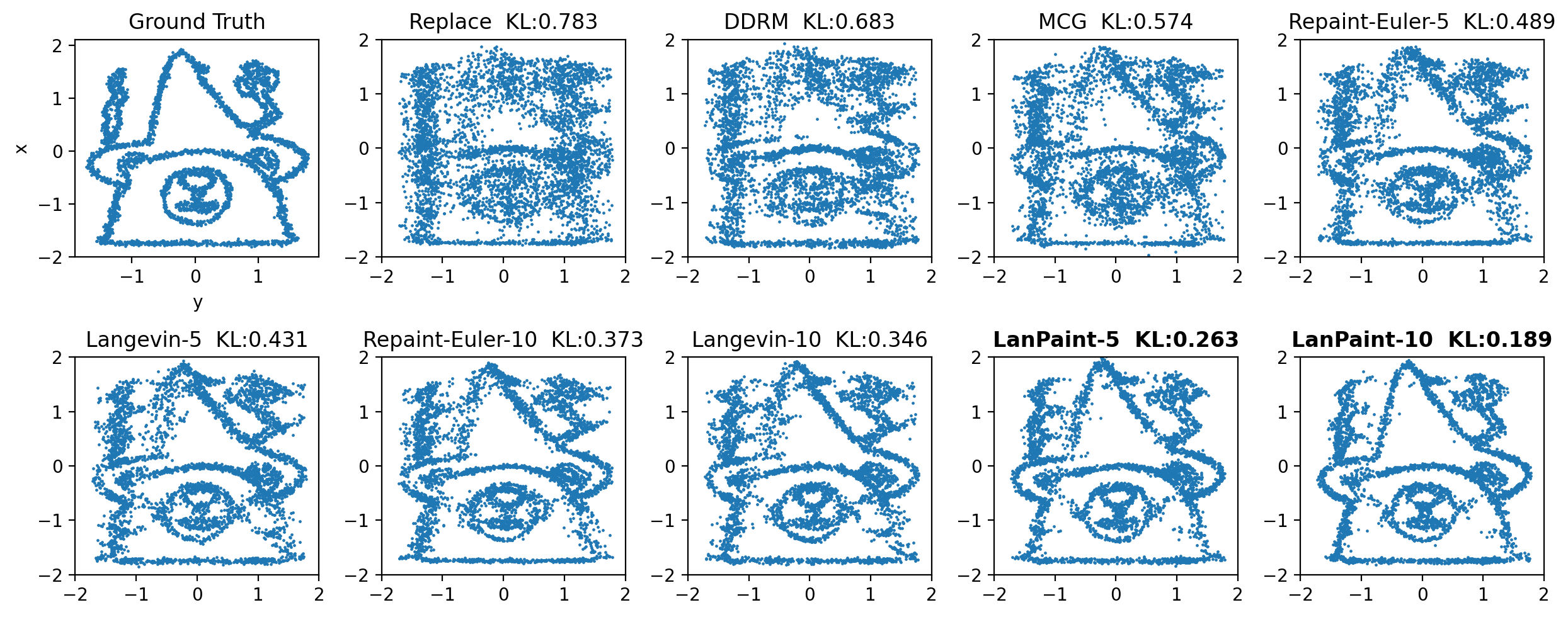
Figure 3: Inpainted samples and KL divergence for inpainting methods on a synthetic Gaussian mixture (MOE) distribution (Section 5.1). The top-left panel displays ground truth MOE samples; other panels show samples with fixed $y$ components and inpainted $x$ values. LanPaint achieves the lowest KL divergence, demonstrating superior performance.

Avoidance of Local Maxima. Figure 2 illustrates the BiG score’s ability to avoid local maxima during sampling. As the number of diffusion steps decreases (right to left), the Langevin method increasingly traps samples (red points) in local maxima, particularly along the dashed lines, even with fast Langevin dynamics (second panel). In contrast, the first panel shows that the BiG score enables the sampler to escape these traps and converge toward the global structure of the target distribution.

Convergence Speed. We quantify the convergence speed gains provided by FLD. Figure 5 compares the convergence of FLD to the original Langevin dynamics 11, demonstrating a $4$ times improvement in convergence speed. This acceleration is critical for practical applications, as it enables LanPaint to achieve high-quality results with fewer inner iterations per diffusion steps.

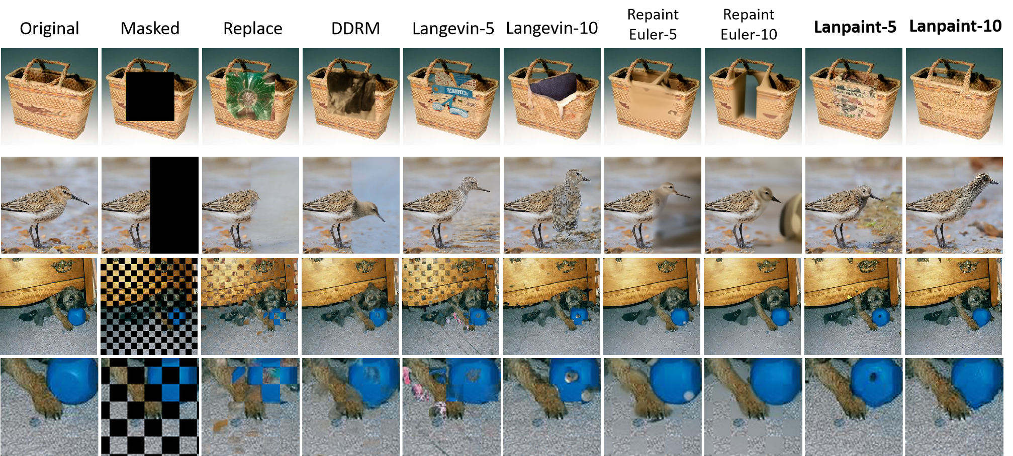
Figure 4: Visual comparisons on ImageNet-256 for center box, half, and checkerboard masks (top to bottom). Numbers 5 and 10 denote the inner iteration counts for RePaint, Langevin, and LanPaint. The bottom row zooms into the checkerboard results (third row), highlighting LanPaint’s superior coherence and texture fidelity compared to baselines, which exhibit visible checkerboard artifacts.

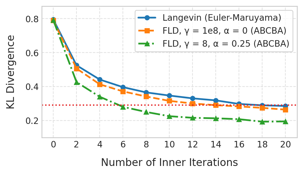
Figure 5: Convergence Comparison (Experiment 5.1): Original Langevin dynamics (solved by Euler-Maruyama scheme) vs FLD (solved by ABCBA operator splitting) at step size $0.05$. The reference case (FLD: $\gamma\to\infty$, $\alpha=0$) matches Langevin’s convergence rate, ensuring a fair comparison (minor KL differences arise from numerical scheme variations). FLD ($\gamma=8$, $\alpha=0.25$) achieves the same KL divergence in 6 steps as Langevin does in 20 steps, demonstrating a 4$\times$ improvement in convergence speed.

Contributions of BiG score and FLD. Our ablation study (Appendix E) demonstrates that both the BiG score and FLD independently enhance sampling performance in LanPaint, with their combination achieving optimal results. Detailed quantitative comparisons, including step-wise results, are provided in Table 2.

5.2 CelebA-HQ-256

We validate LanPaint on the the CelebA-HQ-256 (Liu et al., 2015) dataset to assess its effectiveness in reconstructing masked regions within a latent diffusion framework. The goal is to ensure reconstructed outputs are both visually coherent and faithful to the underlying data distribution.

We use a pre-trained latent diffusion model (Rombach et al., 2021), testing inpainting under fixed sampling budgets (5/10 steps) and diverse mask geometries. Performance is quantified via LPIPS (Zhang et al., 2018) for perceptual fidelity, with comparisons to prior strategies (Lugmayr et al., 2022; Janati et al., 2024). More details are in Appendix D and F.

Table 1 ablates LanPaint’s components on CelebA-HQ-256: combining the BiG score and FLD achieves optimal performance on box and checkerboard masks. LanPaint-5 variants in general achieves comparable results to LanPaint-10 variants (e.g., 0.190 vs. 0.189 on checkerboard masks), demonstrating that 5 steps suffice for high-quality inpainting. Performance on half masks, however, shows greater variance, with FLD-only LanPaint performing best. We attribute this to the half mask’s larger unmasked region, which introduces ambiguity in pixel generation and amplifies LPIPS variability.

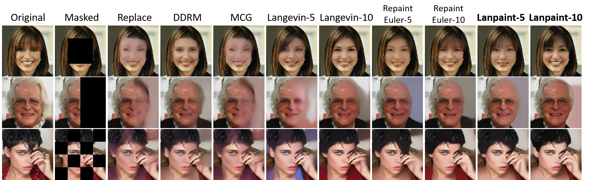
Figure 7: Visual Comparison of inpainting results across various methods on CelebA-HQ 256 dataset: Replace, MCG, DDRM, Langevin-5/10,Repaint-Euler-5/10, and LanPaint-5/10.

LanPaint consistently outperforms existing methods. On checkerboard masks, LanPaint-10 (BiG+FLD) achieves the best LPIPS of 0.189, reducing errors by 7.8% over RePaint-Euler-10 (0.208) and DDRM (0.209). Gains widen on box masks, where LanPaint-10 (BiG+FLD) attains 0.103, surpassing Langevin-10 (0.110) and RePaint-Euler-10 (0.111) by 9.4%. These results highlight LanPaint’s coherence and distribution alignment, demonstrating robust performance with efficient sampling across mask types. The inpainting results are visualized in Appendix Fig.7.

Table 1: LPIPS comparison on CelebA-HQ-256 and ImageNet for various inpainting setups. Euler Discrete Scheduler, 20 steps. Lower LPIPS values indicate better perceptual similarity to the ground truth. LanPaint and its variants achieves the best performance in all scenarios.

	CelebA-HQ-256			ImageNet
Method	Box	Half	Checkerboard	Box	Half	Checkerboard
Repaint-Euler-10†	0.111	0.274	0.208	0.216	0.382	0.134
Repaint-Euler-5†	0.116	0.285	0.214	0.218	0.387	0.137
Langevin-10	0.110	0.281	0.205	0.221	0.391	0.231
Langevin-5	0.116	0.293	0.214	0.226	0.389	0.314
DDRM‡	0.112	0.282	0.209	0.215	0.382	0.213
MCG§	0.130	0.296	0.235	-	-	-
Replace¶	0.131	0.303	0.246	0.228	0.378	0.405
LanPaint-5 (BiG score)	0.108	0.281	0.187	0.212	0.369	0.183
LanPaint-10 (BiG score)	0.104	0.277	0.186	0.209	0.371	0.151
LanPaint-5 (FLD)	0.110	0.283	0.207	0.211	0.360	0.214
LanPaint-10 (FLD)	0.106	0.272	0.198	0.203	0.354	0.158
LanPaint-5 (BiG score+FLD)	0.105	0.277	0.190	0.197	0.337	0.147
LanPaint-10 (BiG score+FLD)	0.103	0.277	0.189	0.193	0.338	0.128

$\dagger$(Lugmayr et al., 2022), $\ddagger$(Kawar et al., 2022), $\S$(Chung et al., 2022b), $\P$(Song & Ermon, 2019b).

5.3 ImageNet-256

We evaluate LanPaint on ImageNet-256 (Deng et al., 2009) using a pretrained diffusion model (Dhariwal & Nichol, 2021), adopting the LPIPS metric and framework from Sec. 5.2. Due to the pre-trained model’s incompatibility with functorch’s per-sample gradients, MCG is excluded. Visualization are provided in Fig.4.

LanPaint outperforms baselines across structured masks (Table 1). For box masks, LanPaint-10 (BiG+FLD) achieves the best LPIPS of 0.193, reducing errors by 10.2% and 10.6% over DDRM (0.215) and Repaint-Euler-10 (0.216). Remarkably, LanPaint-5 (BiG+FLD) nearly matches this performance (0.197 LPIPS) with half the steps. On checkerboard masks, LanPaint-10 (BiG+FLD) attains 0.128 LPIPS—4.5% better than Repaint-Euler-10 (0.134) and 40% better than DDRM (0.213).

On ImageNet, the Langevin-5 and 10 underperforms RePaints, unlike on CelebA. This stems from our reduced step size (0.06→0.04), necessary to align with the pretrained model’s timestep schedule and prevent divergent behavior of the Langevin-5 and 10. Even with this constraint, our LanPaint—using the same reduced step size for fair comparison—surpasses RePaint: LanPaint-10 (BiG+FLD) achieves 0.128 LPIPS vs RePaint-Euler-10’s 0.134 on checkerboard masks. This resilience highlights LanPaint’s robustness under non-ideal step sizes.

5.4 Stable Diffusion

To evaluate LanPaint’s effectiveness in real-world generative settings, we conduct qualitative outpainting experiments using Stable Diffusion v1.4 (Rombach et al., 2021) and AnythingV5 (Yuno779, 2023). A circular mask is applied to selected images, and various inpainting methods are compared. All methods use an Euler Discrete sampler with 20 diffusion steps, while RePaint, Langevin, and LanPaint perform 5 inner iterations per step.

To rigorously assess inpainting performance, we deliberately use prompts that significantly deviate from the original image content, making the task more challenging. For example, given an original medieval fantasy portrait, we prompt the model to generate a ”futuristic cityscape”. This setup tests each method’s ability to produce semantically coherent and contextually integrated completions while maintaining smooth transitions with the known image regions.

Figure 1 presents the inpainting results. Replace, MCG, and DDRM often struggle with contextual blending, producing artifacts and incoherent transitions. RePaint and Langevin improve consistency but sometimes fail to properly integrate new content, resulting in visible boundaries. LanPaint, however, achieves the most visually coherent and semantically relevant completions, seamlessly adapting the masked regions to the given prompts while preserving stylistic and structural consistency. These results validate LanPaint’s superiority in guided diffusion inpainting, particularly under challenging prompt conditions.

6 Discussion

LanPaint achieves efficient, high-quality inpainting across diverse scenarios—from synthetic Gaussian mixtures to real-world Stable Diffusion outpainting—while maintaining computational efficiency. Two key innovations drive this performance: the BiG score, which mitigates local maxima trapping by bidirectional feedback, and FLD, which accelerates convergence of Langevin dynamics. Together, these components position LanPaint as a practical tool for fast and precise image editing.

LanPaint’s training-free design enables plug-and-play inpainting on diverse, community-trained diffusion models without retraining or additional data. Its compatibility with ODE-based samplers further broadens accessibility, allowing users with varying computational resources to perform high-quality inpainting edits.

By framing inpainting as a conditional sampling problem, LanPaint extends beyond images to structured completion tasks. Unlike methods relying on image-specific heuristics, it performs exact conditional inference without domain assumptions, enabling future applications in diverse modalities like text and audio, where coherent generation from partial observations is also critical.

Limitation. LanPaint resamples $x_{t}$ and $y_{t}$ at each diffusion step, breaking continuity between steps. This favors first-order ODE samplers (e.g., Euler) or exponential integrators (e.g., DPM (Lu et al., 2022)) but limits compatibility with interpolation-based like Linear Multi-Step samplers.

Future development. Adopting the Karras notation (Karras et al., 2022) could possibly improve LanPaint’s performance. This observation stems from behavioral differences between Langevin method and RePaint, which arise from discrepancies in implementation. Notably, RePaint-Euler’s use of Karras notation demonstrates greater robustness, suggesting that similar adaptations could enhance LanPaint’s efficacy.

Impact Statement

This work presents a training-free inpainting method that advances generative AI and image editing, with applications in creative industries and digital restoration. The authors emphasize the importance of ethical safeguards to prevent misuse and address potential biases.

Appendix A The Denoising Diffusion Probabilistic Model (DDPMs)

DDPMs (Ho et al., 2020) are models that generate high-quality images from noise via a sequence of denoising steps. Denoting images as random variable $\mathbf{x}$ of the probabilistic density distribution $p(\mathbf{x})$, the DDPM aims to learn a model distribution that mimics the image distribution $p(\mathbf{x})$ and draw samples from it. The training and sampling of the DDPM utilize two diffusion process: the forward and the backward diffusion process.

The forward diffusion process of the DDPM provides necessary information to train a DDPM. It gradually adds noise to existing images $\mathbf{x}_{0}\sim p(x)$ using the Ornstein–Uhlenbeck diffusion process (OU process) (Uhlenbeck & Ornstein, 1930) within a finite time interval $t\in[0,T]$. The OU process is defined by the stochastic differential equation (SDE):

$$d\mathbf{x}_{t}=-\frac{1}{2}\mathbf{x}_{t}dt+d\mathbf{W}_{t},$$ (19)

in which $t$ is the forward time of the diffusion process, $\mathbf{x}_{t}$ is the noise contaminated image at time $t$, and $\mathbf{W}_{t}$ is a standard Brownian motion. The standard Brownian motion formally satisfies $d\mathbf{W}_{t}=\sqrt{dt}\boldsymbol{\epsilon}$ with $\boldsymbol{\epsilon}$ be a standard Gaussian noise. In practice, the OU process is numerically discretized into the variance-preserving (VP) form (Song et al., 2020b):

$$\mathbf{x}_{i}=\sqrt{1-\beta_{i-1}}\mathbf{x}_{i-1}+\sqrt{\beta_{i-1}}\boldsymbol{\epsilon}_{i-1},$$ (20)

where $i=1,\cdots,n$ is the number of the time step, $\beta_{i}$ is the step size of each time step, $\mathbf{x}_{i}$ is image at $i$th time step with time $t_{i}=\sum_{j=0}^{i-1}\beta_{j}$, $\boldsymbol{\epsilon}_{i}$ is standard Gaussian random variable. The time step size usually takes the form $\beta_{i}=\frac{i(b_{2}-b_{1})}{n-1}+b_{1}$ where $b_{1}=10^{-4}$ and $b_{2}=0.02$. Note that our interpretation of $\beta$ differs from that in (Song et al., 2020b), treating $\beta$ as a varying time-step size to solve the autonomous SDE (19) instead of a time-dependent SDE. Our interpretation holds as long as every $\beta_{i}^{2}$ is negligible and greatly simplifies future analysis. The discretized OU process (20) adds a small amount of Gaussian noise to the image at each time step $i$, gradually contaminating the image until $\mathbf{x}_{n}\sim\mathcal{N}(\mathbf{0},I)$.

Training a DDPM aims to recover the original image $x_{0}$ from one of its contaminated versions $x_{i}$. In this case (20) could be rewritten into the form

$$\mathbf{x}_{i}=\sqrt{\bar{\alpha}_{i}}\mathbf{x}_{0}+\sqrt{1-\bar{\alpha}_{i}}\bar{\boldsymbol{\epsilon}}_{i};\quad 1\leq i\leq n,$$ (21)

where $\bar{\alpha}_{i}=\prod_{j=0}^{i-1}(1-\beta_{j})$ is the weight of contamination and $\bar{\boldsymbol{\epsilon}}_{i}$ is a standard Gaussian random noise to be removed. This equation tells us that the distribution of $\mathbf{x}_{i}$ given $\mathbf{x}_{0}$ is a Gaussian distribution

$$p(\mathbf{x}_{i}|\mathbf{x}_{0})=\mathcal{N}(\mathbf{x}|\sqrt{\bar{\alpha}_{i}}\mathbf{x}_{0},(1-\bar{\alpha}_{i})I),$$ (22)

and the noise $\bar{\boldsymbol{\epsilon}}_{i}$ is related to the its score function

$$\bar{\boldsymbol{\epsilon}}_{i}=-\sqrt{1-\bar{\alpha}_{i}}\mathbf{s}(\mathbf{x}_{i}|\mathbf{x}_{0},t_{i}),$$ (23)

where $\mathbf{s}(\mathbf{x}_{i}|\mathbf{x}_{0},t_{i})=\nabla_{\mathbf{x}_{i}}\log p(\mathbf{x}_{i}|\mathbf{x}_{0})$ is the score of the density $p(\mathbf{x}_{i}|\mathbf{x}_{0})$ at $\mathbf{x}_{i}$.

DDPM aims to removes the noise $\bar{\boldsymbol{\epsilon}}_{i}$ from $\mathbf{x}_{i}$ by training a denoising neural network $\boldsymbol{\epsilon}_{\theta}(\mathbf{x},t_{i})$ to predict and remove the noise $\bar{\boldsymbol{\epsilon}}_{i}$. This means that DDPM minimizes the denoising objective (Ho et al., 2020):

$$\begin{split}L_{denoise}(\boldsymbol{\epsilon}_{\theta})&=\frac{1}{n}\sum_{i=1}^{n}\mathbf{E}_{\mathbf{x}_{0}\sim p(\mathbf{x})}\mathbf{E}_{\bar{\boldsymbol{\epsilon}}_{i}\sim\mathcal{N}(\mathbf{0},I)}\|\bar{\boldsymbol{\epsilon}}_{i}-\boldsymbol{\epsilon}_{\theta}(\mathbb{x}_{i},t_{i})\|_{2}^{2}.\end{split}$$ (24)

This is equivalent to, with the help of (23) and tricks in (Vincent, 2011), a denoising score matching objective

$$\begin{split}L_{denoise}(\boldsymbol{\epsilon}_{\theta})&=\frac{1}{n}\sum_{i=1}^{n}(1-\bar{\alpha}_{i})\mathbf{E}_{\mathbf{x_{i}}\sim p(\mathbf{x}_{i})}\|\mathbf{s}(\mathbf{x}_{i},t_{i})+\frac{\boldsymbol{\epsilon}_{\theta}(\mathbb{x}_{i},t_{i})}{\sqrt{1-\bar{\alpha}_{i}}}\|_{2}^{2}.\end{split}$$ (25)

where $\mathbf{s}(\mathbf{x},t_{i})=\nabla_{\mathbf{x}_{i}}\log p(\mathbf{x}_{i})|_{\mathbf{x}_{i}=\mathbf{x}}$ is the score function of the density $p(\mathbf{x}_{i})$. This objectives says that the denoising neural network $\boldsymbol{\epsilon}_{\theta}(\mathbf{x},t_{i})$ is trained to approximate a scaled score function $\boldsymbol{\epsilon}(\mathbf{x},t_{i})$ (Yang et al., 2022)

$$\boldsymbol{\epsilon}(\mathbf{x},t_{i})=\operatorname*{argmin}_{\boldsymbol{\epsilon}_{\theta}}L(\boldsymbol{\epsilon}_{\theta})=-\sqrt{1-\bar{\alpha}_{i}}\mathbf{s}(\mathbf{x},t_{i}).$$ (26)

Another useful property we shall exploit later is that for infinitesimal time steps, the contamination weight $\bar{\alpha}_{i}$ is the exponential of the diffusion time $t_{i}$

$$\lim_{\max_{j}\beta_{j}\xrightarrow[]{}0}\bar{\alpha}_{i}\xrightarrow[]{}e^{-t_{i}}.$$ (27)

In this case, the discretized OU process (20) is equivalent to the OU process (19), with the scaled score function $\boldsymbol{\epsilon}(\mathbf{x},t_{i})$

$$\boldsymbol{\epsilon}(\mathbf{x},t)=-\sqrt{1-e^{-t}}\mathbf{s}(\mathbf{x},t),$$ (28)

related to the score function $\mathbf{s}(\mathbf{x},t)$.

The backward diffusion process is used to sample from the DDPM by removing the noise of an image step by step. It is the time reversed version of the OU process, starting at $x_{0^{\prime}}\sim\mathcal{N}(\mathbf{x}|\mathbf{0},I)$, using the reverse of the OU process (Anderson, 1982b):

$$d\mathbf{x}_{t^{\prime}}=\left(\frac{1}{2}\mathbf{x}_{t^{\prime}}+\mathbf{s}(\mathbf{x},T-t^{\prime})\right)dt^{\prime}+d\mathbf{W}_{t^{\prime}},$$ (29)

in which $t^{\prime}\in[0,T]$ is the backward time, $\mathbf{s}(\mathbf{x},T-t^{\prime})=\nabla_{\mathbf{x}_{T-t^{\prime}}}\log p(\mathbf{x}_{T-t^{\prime}})|_{\mathbf{x}}$ is the score function of the density of $\mathbf{x}_{t=T-t^{\prime}}$ in the forward process. In practice, the backward diffusion process is discretized into

$$\mathbf{x}_{i^{\prime}+1}=\frac{\mathbf{x}_{i^{\prime}}+\mathbf{s}(\mathbf{x}_{i^{\prime}},T-t^{\prime}_{i^{\prime}})\beta_{n-i^{\prime}}}{\sqrt{1-\beta_{n-i^{\prime}}}}+\sqrt{\beta_{n-i^{\prime}}}\boldsymbol{\epsilon}_{i^{\prime}},$$ (30)

where $i^{\prime}=0,\cdots,n$ is the number of the backward time step, $\mathbf{x}_{i^{\prime}}$ is image at $i^{\prime}$th backward time step with time $t_{i^{\prime}}^{\prime}=\sum_{j=0}^{i^{\prime}-1}\beta_{n-1-j}=T-t_{n-i^{\prime}}$, and $\mathbf{s}(\mathbf{x}_{i^{\prime}},T-t^{\prime}_{i^{\prime}})$ is estimated by (26). This discretization is consistent with (29) as long as $\beta_{i}^{2}$ are negligible.

The forward and backward process forms a dual pair when total diffusion time $t_{n}$ is large enough and the time step sizes are small enough, at which $p(\mathbf{x}_{n})=\mathcal{N}(\mathbf{0},I)$. In this case the density of $\mathbf{x}_{t}$ in the forward process and the density of $\mathbf{x}_{t^{\prime}}$ in the backward process satisfying the relation

$$p(\mathbf{x}_{t^{\prime}})|_{t^{\prime}=T-t}=p(\mathbf{x}_{t}).$$ (31)

This relation tells us that the discrete backward diffusion process generate image samples approximately from the image distribution

$$p(\mathbf{x}_{n^{\prime}})\approx p(\mathbf{x}_{0})=p(\mathbf{x}),$$ (32)

despite the discretization error and estimation error of the score function $\mathbf{s}(\mathbf{x},t^{\prime})$. An accurate estimation of the score function is one of the key to sample high quality images.

Appendix B The Fokker–Planck Equation and Langevin Dynamics

1. General Relation Between SDEs and the Fokker–Planck Equation

The Fokker–Planck equation describes the time evolution of the probability density $\rho(\mathbf{z},t)$ associated with a stochastic process governed by a stochastic differential equation (SDE). For a general SDE of the form:

$$dz_{i}=h_{i}(\mathbf{z})\,dt+\gamma_{ij}(\mathbf{z})\,dW_{j},$$ (33)

the corresponding Fokker–Planck equation is:

$$\frac{\partial\rho(\mathbf{z},t)}{\partial t}=-\frac{\partial}{\partial z_{i}}\bigl{[}h_{i}(\mathbf{z})\rho(\mathbf{z},t)\bigr{]}+\frac{1}{2}\frac{\partial^{2}}{\partial z_{j}\partial z_{k}}\bigl{[}\gamma_{ji}(\mathbf{z})\gamma_{ki}(\mathbf{z})\rho(\mathbf{z},t)\bigr{]},$$ (34)

where $h_{i}(\mathbf{z})$ is the drift term, $\gamma_{ij}(\mathbf{z})$ is the diffusion matrix, and $dW_{j}$ are independent Wiener processes.

2. Fokker–Planck Equation and Stationary Distribution of the Langevin Dynamics

Consider the SDE:

$$d\mathbf{z}=\nabla_{\mathbf{z}}\log p(\mathbf{z})\,dt+\sqrt{2}\,d\mathbf{W}_{\mathbf{z}}.$$ (35)

The drift term is $h(\mathbf{z})=\nabla_{\mathbf{z}}\log p(\mathbf{z})$, and the diffusion matrix is constant with $\gamma_{ij}=\sqrt{2}\delta_{ij}$. The Fokker–Planck equation becomes:

$$\frac{\partial\rho(\mathbf{z},t)}{\partial t}=-\frac{\partial}{\partial z_{i}}\Big{[}\Big{(}\frac{\partial\log p(\mathbf{z})}{\partial z_{i}}\Big{)}\rho\Big{]}+\frac{\partial^{2}\rho}{\partial z_{i}^{2}}.$$ (36)

At stationarity, $\frac{\partial\rho}{\partial t}=0$, leading to:

$$0=-\frac{\partial}{\partial z_{i}}\Big{[}\Big{(}\frac{\partial\log p(\mathbf{z})}{\partial z_{i}}\Big{)}\rho\Big{]}+\frac{\partial^{2}\rho}{\partial z_{i}^{2}}.$$ (37)

Solving this equation shows that the stationary distribution is:

$$\rho(\mathbf{z})=p(\mathbf{z}),$$ (38)

where $p(\mathbf{z})$ is the target probability distribution.

3. Fokker–Planck Equation and Stationary Distribution of Fast Langevin Dynamics

Now consider the SDE system:

$$d\mathbf{z} =\frac{1}{m}P\mathbf{v}\,dt+\alpha P\nabla_{\mathbf{z}}\log p(\mathbf{z})\,dt+\sqrt{2\alpha P}\,d\mathbf{W}_{\mathbf{z}},$$ (39)

$$d\mathbf{v} =-\frac{\gamma}{m}P\mathbf{v}\,dt+P\nabla_{\mathbf{z}}\log p(\mathbf{z})\,dt+\sqrt{2\gamma P}\,d\mathbf{W}_{\mathbf{v}},$$

where $P$ is a symmetric positive semidefinite matrix. The Fokker–Planck equation for this system is:

$$\frac{\partial\rho(\mathbf{z},\mathbf{v},t)}{\partial t} =-\frac{\partial}{\partial z_{i}}P_{ij}\Big{[}\Big{(}\frac{1}{m}v_{j}+\alpha\frac{\partial\log p(\mathbf{z})}{\partial z_{j}}\Big{)}\rho-\alpha\frac{\partial\rho}{\partial z_{j}}\Big{]}$$ (40)

$$\quad-\frac{\partial}{\partial v_{i}}P_{ij}\Big{[}\Big{(}-\frac{\gamma}{m}v_{j}+\frac{\partial\log p(\mathbf{z})}{\partial z_{j}}\Big{)}\rho-\gamma\frac{\partial\rho}{\partial v_{j}}\Big{]}.$$

To determine the stationary distribution, assume:

$$\rho(\mathbf{z},\mathbf{v})=p(\mathbf{z})\mathcal{N}(\mathbf{v}|\mathbf{0},m\mathbf{I}),$$ (41)

where $p(\mathbf{z})$ is the marginal distribution of $\mathbf{z}$, and $\mathcal{N}(\mathbf{v}|\mathbf{0},m\mathbf{I})$ is a Gaussian distribution with zero mean and covariance $m\mathbf{I}$. Substituting into the Fokker–Planck equation, we find:

$$\frac{\partial\rho(\mathbf{z},\mathbf{v},t)}{\partial t} =-\frac{\partial}{\partial z_{i}}P_{ij}\Big{[}\frac{1}{m}v_{j}p(\mathbf{z})\mathcal{N}(\mathbf{v}|\mathbf{0},m\mathbf{I})\Big{]}-\frac{\partial}{\partial v_{i}}P_{ij}\Big{[}\frac{\partial p(\mathbf{z})}{\partial z_{j}}\mathcal{N}(\mathbf{v}|\mathbf{0},m\mathbf{I})\Big{]}.$$ (42)

Note that $\partial_{v_{i}}\mathcal{N}(\mathbf{v}|\mathbf{0},m\mathbf{I})=-\frac{v_{i}}{m}\mathcal{N}(\mathbf{v}|\mathbf{0},m\mathbf{I})$, therefore these terms cancel, confirming:

$$\rho(\mathbf{z},\mathbf{v})=p(\mathbf{z})\mathcal{N}(\mathbf{v}|\mathbf{0},m\mathbf{I})$$ (43)

is a stationary solution. This implies: 1. $\mathbf{z}$ follows the target distribution $p(\mathbf{z})$, 2. $\mathbf{v}$ is independent of $\mathbf{z}$ and thermalized around zero with variance proportional to $m$.

Thus, the stationary distribution is a decoupled joint distribution where $\mathbf{z}$ governs the spatial distribution, and $\mathbf{v}$ represents a Gaussian thermal velocity. This proves Theorem 4.2.

Appendix C Stationary Distribution of Guided Langevin Dynamics

In this appendix, we prove that the Guided Langevin Dynamics (BiG score) defined in (14) converges to the target distribution

$$\pi(\mathbf{x}_{t},\mathbf{y}_{t})\propto p(\mathbf{x}_{t}\mid\mathbf{y}_{t})\,\frac{p(\mathbf{y}_{t}\mid\mathbf{y}_{0})^{1+\lambda}}{p(\mathbf{y}_{t})^{\lambda}}+o(\sqrt{1-\bar{\alpha}_{t}}),$$

with a negligible deviation as $t\to 0$. The joint dynamics of $\mathbf{x}_{t}$ and $\mathbf{y}_{t}$ are governed by the following stochastic differential equations (SDEs):

$$d\mathbf{x}_{t} =\mathbf{s}_{\mathbf{x}}(\mathbf{x}_{t},\mathbf{y}_{t},t)\,d\tau+\sqrt{2}\,d\mathbf{W}_{\mathbf{x}},$$

$$d\mathbf{y}_{t} =\mathbf{g}_{\lambda}(\mathbf{x}_{t},\mathbf{y}_{t},t)\,d\tau+\sqrt{2}\,d\mathbf{W}_{\mathbf{y}},$$

where the drift term $\mathbf{g}_{\lambda}$ is defined as

$$\mathbf{g}_{\lambda}(\mathbf{x}_{t},\mathbf{y}_{t},t)=-\left((1+\lambda)\,\frac{\mathbf{y}_{t}-\sqrt{\bar{\alpha}_{t}}\,\mathbf{y}_{0}}{1-\bar{\alpha}_{t}}+\lambda\,\mathbf{s}_{\mathbf{y}}(\mathbf{x}_{t},\mathbf{y}_{t},t)\right).$$

C.1 Idealized SDE for the Target Distribution

To establish the convergence of BiG score, we first consider an idealized SDE whose invariant distribution is the exact target distribution

$$\pi^{*}(\mathbf{x}_{t},\mathbf{y}_{t})\propto p(\mathbf{x}_{t}\mid\mathbf{y}_{t})\,\frac{p(\mathbf{y}_{t}\mid\mathbf{y}_{0})^{1+\lambda}}{p(\mathbf{y}_{t})^{\lambda}}.$$

The drift term of this idealized SDE is given by the gradient of the log-probability:

$$\mathbf{f}^{*}(\mathbf{x}_{t},\mathbf{y}_{t})=\nabla_{\mathbf{x}_{t},\mathbf{y}_{t}}\left[\log p(\mathbf{x}_{t}\mid\mathbf{y}_{t})+(1+\lambda)\log p(\mathbf{y}_{t}\mid\mathbf{y}_{0})-\lambda\log p(\mathbf{y}_{t})\right].$$

Expanding this, we obtain:

$$\mathbf{f}^{*}(\mathbf{x}_{t},\mathbf{y}_{t})=\left(\mathbf{s}^{*}_{\mathbf{x}},\mathbf{s}^{*}_{\mathbf{y}}\right),$$

where

$$\mathbf{s}^{*}_{\mathbf{x}} =\mathbf{s}_{\mathbf{x}}(\mathbf{x}_{t},\mathbf{y}_{t},t),$$

$$\mathbf{s}^{*}_{\mathbf{y}} =(1+\lambda)\,\nabla_{\mathbf{y}_{t}}\log p(\mathbf{x}_{t}\mid\mathbf{y}_{t})+(1+\lambda)\,\nabla_{\mathbf{y}_{t}}\log p(\mathbf{y}_{t}\mid\mathbf{y}_{0})-\lambda\,\nabla_{\mathbf{y}_{t}}\log p(\mathbf{x}_{t},\mathbf{y}_{t}).$$

Using the fact that $p(\mathbf{y}_{t}\mid\mathbf{y}_{0})=\mathcal{N}(\mathbf{y}_{t}\mid\sqrt{\bar{\alpha}_{t}}\,\mathbf{y}_{0},(1-\bar{\alpha}_{t})\mathbf{I})$, we simplify $\mathbf{s}^{*}_{\mathbf{y}}$ to:

$$\mathbf{s}^{*}_{\mathbf{y}}=(1+\lambda)\,\nabla_{\mathbf{y}_{t}}\log p(\mathbf{x}_{t}\mid\mathbf{y}_{t})-(1+\lambda)\,\frac{\mathbf{y}_{t}-\sqrt{\bar{\alpha}_{t}}\,\mathbf{y}_{0}}{1-\bar{\alpha}_{t}}-\lambda\,\nabla_{\mathbf{y}_{t}}\log p(\mathbf{x}_{t},\mathbf{y}_{t}).$$

C.2 Comparison with BiG score Drift Term

To connect the idealized SDE with the BiG score dynamics, we analyze the relationship between $\mathbf{s}^{*}_{\mathbf{y}}$ and $\mathbf{g}_{\lambda}$. Define the following quantities:

$$r_{t} =\mathbb{E}_{p(\mathbf{x}_{t},\mathbf{y}_{t})}\left\|\frac{\mathbf{y}_{t}-\sqrt{\bar{\alpha}_{t}}\,\mathbf{y}_{0}}{1-\bar{\alpha}_{t}}\right\|_{2},$$

$$s_{t} =\mathbb{E}_{p(\mathbf{x}_{t},\mathbf{y}_{t})}\left\|\nabla_{\mathbf{y}_{t}}\log p(\mathbf{x}_{t}\mid\mathbf{y}_{t})\right\|_{2},$$

$$\mathbf{s}_{\text{cond}} =\frac{r_{t}}{s_{t}}\,\nabla_{\mathbf{y}_{t}}\log p(\mathbf{x}_{t}\mid\mathbf{y}_{t}).$$

Here, $\mathbf{s}_{\text{cond}}$ is a rescaled version of $\nabla_{\mathbf{y}_{t}}\log p(\mathbf{x}_{t}\mid\mathbf{y}_{t})$ that matches the order of magnitude of $\frac{\mathbf{y}_{t}-\sqrt{\bar{\alpha}_{t}}\,\mathbf{y}_{0}}{1-\bar{\alpha}_{t}}$. Substituting these definitions into $\mathbf{s}^{*}_{\mathbf{y}}$, we obtain:

$$\mathbf{s}^{*}_{\mathbf{y}}=(1+\lambda)\,\frac{s_{t}}{r_{t}}\,\mathbf{s}_{\text{cond}}+\mathbf{g}_{\lambda}(\mathbf{x}_{t},\mathbf{y}_{t},t).$$

Thus, the idealized drift term $\mathbf{f}^{*}(\mathbf{x}_{t},\mathbf{y}_{t})$ can be expressed as:

$$\mathbf{f}^{*}(\mathbf{x}_{t},\mathbf{y}_{t})=\left(\mathbf{s}_{\mathbf{x}}(\mathbf{x}_{t},\mathbf{y}_{t},t),\,\mathbf{g}_{\lambda}(\mathbf{x}_{t},\mathbf{y}_{t},t)\right)+\frac{s_{t}}{r_{t}}\,\left(\mathbf{0},\,\mathbf{s}_{\text{cond}}\right).$$

C.3 Perturbation Between Ideal and BiG score Scores

To quantify the deviation between the idealized score $\mathbf{s}^{*}_{\mathbf{y}}$ and the BiG score score $\mathbf{g}_{\lambda}$, we analyze the scaling relationship between the terms $\frac{s_{t}}{r_{t}}$ and $\sqrt{1-\bar{\alpha}_{t}}$. Recall that $s_{t}$ and $r_{t}$ are defined as:

$$r_{t} =\mathbb{E}_{p(\mathbf{x}_{t},\mathbf{y}_{t})}\left\|\frac{\mathbf{y}_{t}-\sqrt{\bar{\alpha}_{t}}\,\mathbf{y}_{0}}{1-\bar{\alpha}_{t}}\right\|_{2},$$

$$s_{t} =\mathbb{E}_{p(\mathbf{x}_{t},\mathbf{y}_{t})}\left\|\nabla_{\mathbf{y}_{t}}\log p(\mathbf{x}_{t}\mid\mathbf{y}_{t})\right\|_{2}.$$

From the relationship between the score function and the noise term in diffusion models (see (28)), we have:

$$\boldsymbol{\epsilon}(\mathbf{x},t)=-\sqrt{1-\bar{\alpha}_{t}}\,\mathbf{s}(\mathbf{x},t),$$

where $\bar{\alpha}_{t}=e^{-t}$. This implies that the score function $\mathbf{s}(\mathbf{x},t)$ can be expressed as:

$$\mathbf{s}(\mathbf{x},t)=-\frac{\boldsymbol{\epsilon}(\mathbf{x},t)}{\sqrt{1-\bar{\alpha}_{t}}}.$$

To proceed, we make the following assumption about the noise term $\boldsymbol{\epsilon}(\mathbf{x},t)$:

Assumption C.1.

The expected $L_{2}$ norm of the noise term $\boldsymbol{\epsilon}(\mathbf{x},t)$ is a positive bounded value, i.e., there exists a constant $C>0$ such that

$$\mathbb{E}_{p(\mathbf{x},t)}\left\|\boldsymbol{\epsilon}(\mathbf{x},t)\right\|_{2}=C.$$

Under Assumption C.1, we can derive the scaling behavior of $s_{t}$ and $r_{t}$:

1. **Scaling of $s_{t}$:** Since $\nabla_{\mathbf{y}_{t}}\log p(\mathbf{x}_{t}\mid\mathbf{y}_{t})$ is a score function, it follows the same scaling as $\mathbf{s}(\mathbf{x},t)$. Thus,

$$s_{t}=\mathbb{E}_{p(\mathbf{x}_{t},\mathbf{y}_{t})}\left\|\nabla_{\mathbf{y}_{t}}\log p(\mathbf{x}_{t}\mid\mathbf{y}_{t})\right\|_{2}\sim\frac{C}{\sqrt{1-\bar{\alpha}_{t}}}.$$

2. **Scaling of $r_{t}$:** The term $\frac{\mathbf{y}_{t}-\sqrt{\bar{\alpha}_{t}}\,\mathbf{y}_{0}}{1-\bar{\alpha}_{t}}$ represents the normalized deviation of $\mathbf{y}_{t}$ from its mean. For small $1-\bar{\alpha}_{t}$, this term scales as:

$$r_{t}=\mathbb{E}_{p(\mathbf{x}_{t},\mathbf{y}_{t})}\left\|\frac{\mathbf{y}_{t}-\sqrt{\bar{\alpha}_{t}}\,\mathbf{y}_{0}}{1-\bar{\alpha}_{t}}\right\|_{2}\sim\frac{C^{\prime}}{1-\bar{\alpha}_{t}},$$

where $C^{\prime}>0$ is another constant.

3. **Ratio $\frac{s_{t}}{r_{t}}$:** Combining the scaling behaviors of $s_{t}$ and $r_{t}$, we obtain:

$$\frac{s_{t}}{r_{t}}\sim\frac{C/\sqrt{1-\bar{\alpha}_{t}}}{C^{\prime}/(1-\bar{\alpha}_{t})}=\frac{C}{C^{\prime}}\sqrt{1-\bar{\alpha}_{t}}.$$

Thus, $\frac{s_{t}}{r_{t}}$ scales as $\mathcal{O}(\sqrt{1-\bar{\alpha}_{t}})$.

C.4 Fokker-Planck Equation Analysis

The Fokker–Planck equation (34) describes the time evolution of the probability density $\rho(\mathbf{z},\tau)$ associated with a stochastic process governed by a stochastic differential equation (SDE). For a general SDE of the form:

$$dz_{i}=h_{i}(\mathbf{z})\,d\tau+\gamma_{ij}(\mathbf{z})\,dW_{j},$$

the corresponding Fokker–Planck equation can be written in operator form as:

$$\frac{\partial\rho(\mathbf{z},\tau)}{\partial\tau}=\mathcal{L}\rho(\mathbf{z},\tau),$$

where $\mathcal{L}$ is the Fokker-Planck operator, defined as:

$$\mathcal{L}=-\nabla\cdot\bigl{[}\mathbf{h}(\mathbf{z})\,\cdot\bigr{]}+\frac{1}{2}\nabla\cdot\bigl{[}\mathbf{D}(\mathbf{z})\nabla\cdot\bigr{]}.$$

Here, $\mathbf{h}(\mathbf{z})$ is the drift vector, $\mathbf{D}(\mathbf{z})=\gamma(\mathbf{z})\gamma(\mathbf{z})^{\top}$ is the diffusion matrix, and $\nabla\cdot$ denotes the divergence operator.

C.4.1 Fokker-Planck Operator for BiG score

The BiG score dynamics are governed by the following SDEs:

$$d\mathbf{x}_{t} =\mathbf{s}_{\mathbf{x}}(\mathbf{x}_{t},\mathbf{y}_{t},t)\,d\tau+\sqrt{2}\,d\mathbf{W}_{\mathbf{x}},$$

$$d\mathbf{y}_{t} =\mathbf{g}_{\lambda}(\mathbf{x}_{t},\mathbf{y}_{t},t)\,d\tau+\sqrt{2}\,d\mathbf{W}_{\mathbf{y}},$$

where $\mathbf{g}_{\lambda}(\mathbf{x}_{t},\mathbf{y}_{t},t)$ is defined as:

$$\mathbf{g}_{\lambda}(\mathbf{x}_{t},\mathbf{y}_{t},t)=-\left((1+\lambda)\,\frac{\mathbf{y}_{t}-\sqrt{\bar{\alpha}_{t}}\,\mathbf{y}_{0}}{1-\bar{\alpha}_{t}}+\lambda\,\mathbf{s}_{\mathbf{y}}(\mathbf{x}_{t},\mathbf{y}_{t},t)\right).$$

The corresponding Fokker-Planck operator for the BiG score is:

$$\mathcal{L}_{\text{BiG score}}=-\nabla_{\mathbf{x}_{t}}\cdot\bigl{[}\mathbf{s}_{\mathbf{x}}(\mathbf{x}_{t},\mathbf{y}_{t},t)\,\cdot\bigr{]}-\nabla_{\mathbf{y}_{t}}\cdot\bigl{[}\mathbf{g}_{\lambda}(\mathbf{x}_{t},\mathbf{y}_{t},t)\,\cdot\bigr{]}+\nabla^{2},$$

where $\nabla^{2}$ is the Laplacian operator.

C.4.2 Fokker-Planck Operator for the Idealized SDE

The idealized SDE, which has the target distribution $\pi(\mathbf{x}_{t},\mathbf{y}_{t})$ as its stationary distribution, is given by:

$$d(\mathbf{x}_{t},\mathbf{y}_{t})=\mathbf{f}^{*}(\mathbf{x}_{t},\mathbf{y}_{t})\,d\tau+\sqrt{2}\,d\mathbf{W},$$

where $\mathbf{f}^{*}(\mathbf{x}_{t},\mathbf{y}_{t})=\bigl{(}\mathbf{s}^{*}_{\mathbf{x}},\mathbf{s}^{*}_{\mathbf{y}}\bigr{)}$ is the drift term. The corresponding Fokker-Planck operator for the idealized SDE is:

$$\mathcal{L}_{\text{ideal}}=-\nabla_{\mathbf{x}_{t}}\cdot\bigl{[}\mathbf{s}_{\mathbf{x}}(\mathbf{x}_{t},\mathbf{y}_{t},t)\,\cdot\bigr{]}-\nabla_{\mathbf{y}_{t}}\cdot\bigl{[}\mathbf{s}^{*}_{\mathbf{y}}(\mathbf{x}_{t},\mathbf{y}_{t},t)\,\cdot\bigr{]}+\nabla^{2}.$$

C.4.3 Deviation Between BiG score and Idealized SDE

The key difference between the BiG score and the idealized SDE lies in their drift terms. Specifically, the drift term $\mathbf{s}^{*}_{\mathbf{y}}$ for the idealized SDE can be expressed in terms of the BiG score drift term $\mathbf{g}_{\lambda}$ as:

$$\mathbf{s}^{*}_{\mathbf{y}}=(1+\lambda)\,\frac{s_{t}}{r_{t}}\,\mathbf{s}_{\text{cond}}+\mathbf{g}_{\lambda}(\mathbf{x}_{t},\mathbf{y}_{t},t),$$

where $\mathbf{s}_{\text{cond}}=\frac{r_{t}}{s_{t}}\,\nabla_{\mathbf{y}_{t}}\log p(\mathbf{x}_{t}\mid\mathbf{y}_{t})$. Thus, the difference between the Fokker-Planck operators for the BiG score and the idealized SDE is:

$$\mathcal{L}_{\text{BiG score}}-\mathcal{L}_{\text{ideal}}=-\nabla_{\mathbf{y}_{t}}\cdot\left[(1+\lambda)\,\frac{s_{t}}{r_{t}}\,\mathbf{s}_{\text{cond}}\,\cdot\right].$$

This additional term represents the perturbation between the BiG score and the idealized SDE.

C.4.4 Analysis Using Dyson’s Formula

To analyze the deviation of the solutions to the Fokker-Planck equations, we use Dyson’s Formula (Evans & Morriss, 2008), a powerful tool in the study of perturbed differential equations. Dyson’s Formula expresses the solution to a perturbed differential equation in terms of the unperturbed solution. Specifically, for a differential equation of the form

$$\frac{\partial\rho(\mathbf{z},\tau)}{\partial\tau}=(\mathcal{L}_{0}+\mathcal{L}_{1})\rho(\mathbf{z},\tau),$$

where $\mathcal{L}_{0}$ is the unperturbed operator and $\mathcal{L}_{1}$ is a perturbation, the solution can be written as

$$\rho(\mathbf{z},\tau)=e^{(\mathcal{L}_{0}+\mathcal{L}_{1})\tau}\rho(\mathbf{z},0)=e^{\mathcal{L}_{0}\tau}\rho(\mathbf{z},0)+\int_{0}^{\tau}e^{\mathcal{L}_{0}(\tau-s)}\mathcal{L}_{1}\rho(\mathbf{z},s)\,ds.$$

This formula allows us to express the solution to the perturbed equation as the sum of the unperturbed solution and a correction term due to the perturbation.

In our case, the Fokker-Planck equation for the BiG score can be viewed as a perturbation of the idealized Fokker-Planck equation. Let $\rho_{\text{ideal}}(\mathbf{x}_{t},\mathbf{y}_{t},\tau)$ be the solution to the idealized Fokker-Planck equation:

$$\frac{\partial\rho_{\text{ideal}}}{\partial\tau}=\mathcal{L}_{\text{ideal}}\rho_{\text{ideal}}.$$

The solution to the BiG score Fokker-Planck equation can then be written using Dyson’s Formula as:

$$\rho_{\text{BiG score}}(\mathbf{x}_{t},\mathbf{y}_{t},\tau)=\rho_{\text{ideal}}(\mathbf{x}_{t},\mathbf{y}_{t},\tau)+\int_{0}^{\tau}e^{\mathcal{L}_{\text{ideal}}(\tau-s)}\left(\mathcal{L}_{\text{BiG score}}-\mathcal{L}_{\text{ideal}}\right)\rho_{\text{BiG score}}(\mathbf{x}_{t},\mathbf{y}_{t},s)\,ds.$$

Substituting the perturbation term, we obtain:

$$\rho_{\text{BiG score}}(\mathbf{x}_{t},\mathbf{y}_{t},\tau)=\rho_{\text{ideal}}(\mathbf{x}_{t},\mathbf{y}_{t},\tau)-(1+\lambda)\,\frac{s_{t}}{r_{t}}\int_{0}^{\tau}e^{\mathcal{L}_{\text{ideal}}(\tau-s)}\nabla_{\mathbf{y}_{t}}\cdot\left[\mathbf{s}_{\text{cond}}\,\rho_{\text{BiG score}}(\mathbf{x}_{t},\mathbf{y}_{t},s)\right]\,ds.$$

From the analysis in Section C.3, we know that $\frac{s_{t}}{r_{t}}\sim\sqrt{1-\bar{\alpha}_{t}}$. Thus, the deviation term is proportional to $\sqrt{1-\bar{\alpha}_{t}}$.

C.5 Conclusion

As $\tau\to\infty$, the idealized solution $\rho_{\text{ideal}}(\mathbf{x}_{t},\mathbf{y}_{t},\tau)$ converges exponentially to the stationary distribution $\pi^{*}(\mathbf{x}_{t},\mathbf{y}_{t})$, driven by the contractive nature of $\mathcal{L}_{\text{ideal}}$. The BiG score dynamics, governed by $\rho_{\text{BiG score}}$, deviate from $\pi^{*}$ by a term proportional to $\sqrt{1-\bar{\alpha}_{t}}$. This deviation remains bounded due to two key mechanisms:

• Vanishing Perturbation Strength: The ratio $\frac{s_{t}}{r_{t}}\sim\sqrt{1-\bar{\alpha}_{t}}$ shrinks to zero as $t\to 0$.

• Exponential Damping: The semigroup $e^{\mathcal{L}_{\text{ideal}}(\tau-s)}$ suppresses perturbations over time, with decay rates governed by the spectral gap of $\mathcal{L}_{\text{ideal}}$. Hence contributions to the deviation integral are dominated by a finite effective timescale.

Thus, the BiG score dynamics converge to $\pi^{*}(\mathbf{x}_{t},\mathbf{y}_{t})$ with negligible error as $t\to 0$, controlled by the vanishing perturbation of the order $\sqrt{1-\bar{\alpha}_{t}}$. This argument hence proves Theorem 4.1.

Appendix D Implementation

LanPaint

We implement LanPaint using the diffusers package, following Algorithm 1. Hyperparameters are configured as follows: $\gamma=8$, $\alpha=0.25$, $M=1$, $\beta=1$, and $\lambda=10$. The notation LanPaint-5 and LanPaint-10 denotes $N=5$ and $N=10$ sampling steps, respectively. The step size $\eta$ is shared with Langevin dynamics for fair comparison. It is set to $0.03$ and $0.04$ for ImageNet box and checkerboard case to avoid divergence behavior of Langevin method, otherwise set to $0.06$ for all other cases. For fair comparison, we align the step size $d\tau_{F}$ of the Fast Langevin Dynamics (17) with $d\tau_{L}$ of Langevin Dynamics (13) by

$$d\tau_{F}=\sqrt{2Md\tau_{L}},$$

to ensure that they coincide at $\gamma=+\infty$, $P=I$, and $\alpha=0$.

Algorithm 1 LanPaint: Conditional Inpainting with BiG score-FLD Dynamics

Input image $y$, mask $m$, text embeddings $\mathbf{e}$, friction $\gamma$, mass $M$, step size $\eta$, steps $N$, BiG score params $\beta$, $\lambda$ Inpainted image $\mathbf{x}$ Initialize: $\mathbf{z}\leftarrow\text{Random noise}$ *Latent variable $\{\mathbf{y}_{t}\}\leftarrow\text{ForwardDiffuse}(y)$ *Pre-diffused inputs

each timestep $t$ $\mathbf{y}_{t}\leftarrow\text{ForwardDiffusedImage}(t)$

Compute BiG score scores $\epsilon\leftarrow\text{UNet}(\mathbf{z},t,\mathbf{e})$ *Noise predicted by diffusion model $\mathbf{s}_{x}\leftarrow-\epsilon/\sqrt{1-\bar{\alpha}_{t}}$ *score of x $\mathbf{s}_{y}\leftarrow\frac{-(1+\lambda_{g})(\mathbf{z}-\sqrt{\bar{\alpha}_{t}}\mathbf{y})}{(1-\bar{\alpha}_{t})}+\frac{\lambda\epsilon}{\sqrt{1-\bar{\alpha}_{t}}}$ *score of y

Prepare FLD Step Size

$d\tau\leftarrow\min\{\eta\sqrt{1-\bar{\alpha}_{t}},-\log\bar{\alpha}_{t}/2\}$ *Set the step size

$\sigma_{x}\leftarrow 1$, $\sigma_{y}\leftarrow\beta\sqrt{1-\bar{\alpha}_{t}}$ $\eta_{x}\leftarrow d\tau\sigma_{x}$, $\eta_{y}\leftarrow d\tau\sigma_{y}$ *Scale steps using $P=\text{diag}(\sigma_{x},\sigma_{y})$

Align FLD time with Langevin dynamics for Fair Comparison $\eta_{x}\leftarrow\sqrt{2M\eta_{x}}$, $\eta_{y}\leftarrow\sqrt{2M\eta_{y}}$

FLD iteration with ABCBA Operator Splitting $\mathbf{v}_{x,y}\leftarrow\sqrt{M}\xi_{x,y}^{\mathbf{v}}$ *Initialize velocity $\mathbf{z}_{x}\leftarrow\mathbf{z}\odot(1-m)$, $\mathbf{z}_{y}\leftarrow\mathbf{z}\odot m$ *Split variables $k=1$ to $N$ substep in [A-half, B-half, C, B-half, A-half] substep is A-half $\mathbf{v}_{x,y}\leftarrow e^{-\gamma\eta_{x,y}/M}\mathbf{v}_{x,y}+\sqrt{M(1-e^{-2\gamma\eta_{x,y}/M})}\xi_{x,y}$ *$d\mathbf{v}\;=\;-\,\frac{\gamma}{m}\,P\,\mathbf{v}\,d\tau\;+\;\sqrt{2\,\gamma\,P}\;dW_{\mathbf{v}},$ substep is B-half $\mathbf{z}_{x,y}\leftarrow\mathbf{z}_{x,y}+\eta_{x,y}\mathbf{v}_{x,y}/(2M)$ *$d\mathbf{z}\;=\;\frac{1}{m}\,P\,\mathbf{v}\,d\tau$ substep is C $\mathbf{v}_{x,y}\leftarrow\mathbf{v}_{x,y}+\eta_{x,y}\mathbf{s}_{x,y}$ *$d\mathbf{v}\;=\;P\,\mathbf{s}(\mathbf{z})\,d\tau$

$\alpha$ is multiplied by $\eta$ here to limit the step size $\mathbf{z}_{x,y}\leftarrow\mathbf{z}_{x,y}+\alpha\eta_{x,y}^{2}\mathbf{s}_{x,y}+\sqrt{2\alpha\eta_{x,y}^{2}}\xi_{x,y}$ *$d\mathbf{z}\;=\;\;\alpha\,P\,\mathbf{s}(\mathbf{z})\,d\tau+\;\sqrt{2\,\alpha\,P}\;dW_{\mathbf{z}}$ Recombine variables with mask

$\mathbf{z}\leftarrow\mathbf{z}_{x}\odot(1-m)+\mathbf{z}_{y}\odot m$

$\epsilon\leftarrow\text{UNet}(\mathbf{z},t,\mathbf{e})$ *Noise predicted by diffusion model $\mathbf{z}\leftarrow\text{SchedulerStep}(\mathbf{z},\epsilon,t)$ *Predict the next step image with any fast sampler $\mathbf{z}$

Langevin

Langevin sampling is implemented via the Euler-Maruyama discretization of Eq. (11), with step size $\mathrm{d}\tau=\eta\sqrt{1-\bar{\alpha}_{t}}$ ($\eta$ share with LanPaint). This is similar with Algorithm 1 in the concurrent work by Cornwall et al. (Cornwall et al., 2024), except that they use $\mathbf{y}_{t}=\sqrt{\bar{\alpha}_{t}}\mathbf{y}_{0}$ without adding noise. The DCPS method from Janati et al. (Janati et al., 2024) is not implemented due to its dependence on DDPM posterior sampling; adaptation to fast samplers is non-trivial.

DDRM

Our implementation of DDRM follows Equations (7) and (8) in Kawar et al. (Kawar et al., 2022), with $\sigma_{y}=0$, $\mathbf{V}=I$, and $s_{i}=1$ for observed regions $\mathbf{y}$ and $s_{i}=0$ for inpainted regions $\mathbf{x}$. The hyperparameters $\eta=0.7$ and $\eta_{b}=1$ are selected based on the optimal KID scores reported in Table 3 of the reference.

MCG

We adopt MCG as outlined in Algorithm 1 of Chung et al. (Chung et al., 2022b), using $\alpha=0.1/\|\mathbf{y}-P\hat{\mathbf{x}}_{0}\|$ as recommended in Appendix C. Due to incompatibility with gradient computation via functorch in the pre-trained DDPM framework, MCG was not evaluated on ImageNet.

RePaint

We implement RePaint based on Algorithm 1 in Lugmayr et al. (Lugmayr et al., 2022), with modifications to accommodate fast samplers. While the original method was designed for DDPM, we adapt it by replacing the backward sampling step (Line 7) with a Euler Discrete Sample step. Additionally, we set the jump step size to $1$ instead of the default $10$ backward steps recommended in Appendix B of the original work. This adjustment is necessary because fast samplers typically operate with only around $20$ backward sampling steps, making larger jump sizes impractical.

Appendix E Mixture of Gaussian Benchmark

Method	Inner Steps	KL$\downarrow$
LanPaint-5 (BiG score only)	5	0.331
LanPaint-5 (FLD only)	5	0.307
LanPaint-5 (BiG score + FLD)	5	0.255
LanPaint-10 (BiG score only)	10	0.255
LanPaint-10 (FLD only)	10	0.227
LanPaint-10 (BiG score + FLD)	10	0.187

Table 2: Ablation study of LanPaint, showing KL divergence for BiG score and FLD. Lower KL values indicate better sample fidelity.

We construct a synthetic dataset using a black-and-white image (e.g., a wizard bear silhouette shown in Fig.3). The image is converted into a binary mask, and a 500-component Gaussian mixture model (GMM) is fitted to the foreground pixel coordinates. The task is framed as 2D inpainting: given observed $y$-coordinates, infer masked $x$-values. We compare several methods—Replace(Song & Ermon, 2019b), MCG(Chung et al., 2022b), DDRM(Kawar et al., 2022), RePaint(Lugmayr et al., 2022), Langevin, and LanPaint—using an Euler discrete sampler with 20 steps. Performance is quantified via KL divergence between inpainted samples and the ground truth GMM. Specifically, we fit a new GMM to the generated samples and compute its divergence from the original model. Lower KL values indicate higher fidelity to the target distribution.

Contributions of BiG score and FLD. Table 2 analyzes the contributions of BiG score and FLD within LanPaint. Both components independently reduce KL divergence, and their combination yields the best results. Specifically, with 5 diffusion steps, LanPaint (BiG score+FLD) achieves $\mathrm{KL}=0.255$, outperforming BiG score-only or FLD-only variants. At 10 steps, LanPaint (BiG score+FLD) further improves to $\mathrm{KL}=0.187$. These findings show that both guided updates (BiG score) and faster convergence (FLD) are crucial to achieving superior performance.

Appendix F CelebA-HQ-256

We test LanPaint on a pre-trained latent diffusion model (Rombach et al., 2021) for CelebA-HQ-256, evaluating inpainting performance on 1,000 validation images with three distinct masks: center box, half, and checkerboard. These masks test LanPaint’s adaptability to varying masked region geometries. We compare multiple inpainting strategies. For diffusion model sampling, we use a 20-step Euler discrete schedule adopted from the diffusers package (von Platen et al., 2022). To standardize comparisons, all iterative methods (RePaint, Langevin, LanPaint) are allocated a fixed sampling budget of 5 or 10 inner steps during inference. Following the prior works (Lugmayr et al., 2022; Janati et al., 2024), reconstruction fidelity is quantified using the Learned Perceptual Image Patch Similarity (LPIPS) (Zhang et al., 2018), where lower scores indicate higher perceptual alignment with ground-truth images. Results are averaged across all samples for robustness.

Appendix G Stable Diffusion Visualizations

Fig.8 and Fig.9 provide more visualizations generated by stable diffusion models.

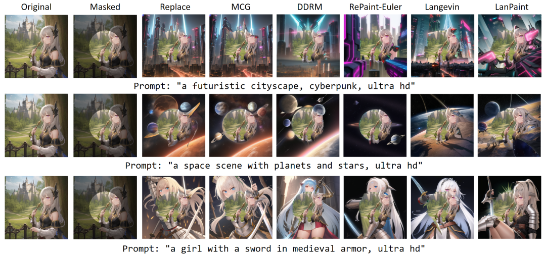
Figure 8: Comparison of inpainting results across various methods: Replace, MCG, DDRM, Repaint-Euler-5, Langevin-5, and LanPaint-5. The leftmost column shows the original and masked images, while the remaining columns present the inpainted results for different prompts. LanPaint consistently produces visually coherent and semantically aligned results that blend well with the context, avoiding artifacts and mismatches observed in other methods. This highlights LanPaint’s superior performance in inpainting tasks. Model: Anything V5 (Stable Diffusion 1.5) Sampler: Euler Discrete, 20 steps

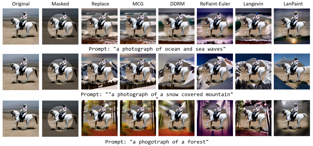
Figure 9: Comparison of inpainting results across various methods: Replace, MCG, DDRM, Repaint-Euler-5, Langevin-5, and LanPaint-5. The leftmost column shows the original and masked images, while the remaining columns present the inpainted results for different prompts. LanPaint consistently produces visually coherent and semantically aligned results that blend well with the context, avoiding artifacts and mismatches observed in other methods. This highlights LanPaint’s superior performance in inpainting tasks. Model: Stable Diffusion 1.4 Sampler: Euler Discrete, 20 steps

References

- AlRachid et al. (2018) AlRachid, H., Mones, L., and Ortner, C. Some remarks on preconditioning molecular dynamics. The SMAI Journal of computational mathematics, 4:57–80, 2018.
- Anderson (1982a) Anderson, B. D. Reverse-time diffusion equation models. Stochastic Processes and their Applications, 12(3):313–326, 1982a.
- Anderson (1982b) Anderson, B. D. O. Reverse-time diffusion equation models. Stochastic Processes and their Applications, 12:313–326, 1982b.
- Avrahami et al. (2023) Avrahami, O., Fried, O., and Lischinski, D. Blended latent diffusion. ACM transactions on graphics (TOG), 42(4):1–11, 2023.
- Betker et al. (2023) Betker, J., Goh, G., Jing, L., Brooks, T., Wang, J., Li, L., Ouyang, L., Zhuang, J., Lee, J., Guo, Y., et al. Improving image generation with better captions, 2023.
- Cardoso et al. (2023) Cardoso, G., Le Corff, S., Moulines, E., et al. Monte carlo guided denoising diffusion models for bayesian linear inverse problems. In The Twelfth International Conference on Learning Representations, 2023.
- Cheng et al. (2018) Cheng, X., Chatterji, N. S., Bartlett, P. L., and Jordan, M. I. Underdamped langevin mcmc: A non-asymptotic analysis. In Conference on learning theory, pp. 300–323. PMLR, 2018.
- Chung et al. (2022a) Chung, H., Kim, J., Mccann, M. T., Klasky, M. L., and Ye, J. C. Diffusion posterior sampling for general noisy inverse problems. arXiv preprint arXiv:2209.14687, 2022a.
- Chung et al. (2022b) Chung, H., Sim, B., Ryu, D., and Ye, J. C. Improving diffusion models for inverse problems using manifold constraints. Advances in Neural Information Processing Systems, 35:25683–25696, 2022b.
- Corneanu et al. (2024) Corneanu, C., Gadde, R., and Martinez, A. M. Latentpaint: Image inpainting in latent space with diffusion models. In Proceedings of the IEEE/CVF Winter Conference on Applications of Computer Vision, pp. 4334–4343, 2024.
- Cornwall et al. (2024) Cornwall, L., Meyers, J., Day, J., Wollman, L. S., Dalchau, N., and Sim, A. Training-free guidance of diffusion models for generalised inpainting, 2024. URL https://openreview.net/forum?id=AC1QLOJK7l.
- Deng et al. (2009) Deng, J., Dong, W., Socher, R., Li, L.-J., Li, K., and Fei-Fei, L. Imagenet: A large-scale hierarchical image database. In 2009 IEEE Conference on Computer Vision and Pattern Recognition, pp. 248–255, 2009. doi: 10.1109/CVPR.2009.5206848.
- Dhariwal & Nichol (2021) Dhariwal, P. and Nichol, A. Diffusion models beat gans on image synthesis. ArXiv, abs/2105.05233, 2021.
- Evans & Morriss (2008) Evans, D. J. and Morriss, G. The microscopic connection, pp. 33–78. Cambridge University Press, 2008.
- FBehrad (2022) FBehrad. Issue #1213: Repaint compatibility with fast samplers. https://github.com/huggingface/diffusers/issues/1213, 2022. Accessed: [Insert Date].
- Grechka et al. (2024) Grechka, A., Couairon, G., and Cord, M. Gradpaint: Gradient-guided inpainting with diffusion models. Computer Vision and Image Understanding, 240:103928, 2024.
- Ho et al. (2020) Ho, J., Jain, A., and Abbeel, P. Denoising diffusion probabilistic models. ArXiv, abs/2006.11239, 2020.
- Janati et al. (2024) Janati, Y., Moufad, B., Durmus, A., Moulines, E., and Olsson, J. Divide-and-conquer posterior sampling for denoising diffusion priors, 2024. URL https://arxiv.org/abs/2403.11407.
- Karras et al. (2022) Karras, T., Aittala, M., Aila, T., and Laine, S. Elucidating the design space of diffusion-based generative models. ArXiv, abs/2206.00364, 2022.
- Kawar et al. (2022) Kawar, B., Elad, M., Ermon, S., and Song, J. Denoising diffusion restoration models. Advances in Neural Information Processing Systems, 35:23593–23606, 2022.
- Langley (2000) Langley, P. Crafting papers on machine learning. In Langley, P. (ed.), Proceedings of the 17th International Conference on Machine Learning (ICML 2000), pp. 1207–1216, Stanford, CA, 2000. Morgan Kaufmann.
- Li et al. (2022) Li, R., Zha, H., and Tao, M. Hessian-free high-resolution nesterov acceleration for sampling. In International Conference on Machine Learning, pp. 13125–13162. PMLR, 2022.
- Liu et al. (2023) Liu, G.-H., Vahdat, A., Huang, D.-A., Theodorou, E. A., Nie, W., and Anandkumar, A. I2sb: Image-to-image schr” odinger bridge. arXiv preprint arXiv:2302.05872, 2023.
- Liu et al. (2022a) Liu, L., Ren, Y., Lin, Z., and Zhao, Z. Pseudo numerical methods for diffusion models on manifolds. ArXiv, abs/2202.09778, 2022a.
- Liu et al. (2022b) Liu, X., Wu, L., Ye, M., and Liu, Q. Let us build bridges: Understanding and extending diffusion generative models. arXiv preprint arXiv:2208.14699, 2022b.
- Liu et al. (2015) Liu, Z., Luo, P., Wang, X., and Tang, X. Deep learning face attributes in the wild. In Proceedings of International Conference on Computer Vision (ICCV), December 2015.
- Lu et al. (2022) Lu, C., Zhou, Y., Bao, F., Chen, J., Li, C., and Zhu, J. Dpm-solver++: Fast solver for guided sampling of diffusion probabilistic models. ArXiv, abs/2211.01095, 2022.
- Lugmayr et al. (2022) Lugmayr, A., Danelljan, M., Romero, A., Yu, F., Timofte, R., and Van Gool, L. Repaint: Inpainting using denoising diffusion probabilistic models. In Proceedings of the IEEE/CVF conference on computer vision and pattern recognition, pp. 11461–11471, 2022.
- Park et al. (2024) Park, S. H., Koh, J. Y., Lee, J., Song, J., Kim, D., Moon, H., Lee, H., and Song, M. Illustrious: an open advanced illustration model. arXiv preprint arXiv:2409.19946, 2024.
- Rombach et al. (2021) Rombach, R., Blattmann, A., Lorenz, D., Esser, P., and Ommer, B. High-resolution image synthesis with latent diffusion models. 2022 IEEE/CVF Conference on Computer Vision and Pattern Recognition (CVPR), pp. 10674–10685, 2021.
- Sohl-Dickstein et al. (2015) Sohl-Dickstein, J. N., Weiss, E. A., Maheswaranathan, N., and Ganguli, S. Deep unsupervised learning using nonequilibrium thermodynamics. ArXiv, abs/1503.03585, 2015.
- Song et al. (2020a) Song, J., Meng, C., and Ermon, S. Denoising diffusion implicit models. ArXiv, abs/2010.02502, 2020a.
- Song & Ermon (2019a) Song, Y. and Ermon, S. Generative modeling by estimating gradients of the data distribution. In Neural Information Processing Systems, 2019a.
- Song & Ermon (2019b) Song, Y. and Ermon, S. Generative modeling by estimating gradients of the data distribution. Advances in neural information processing systems, 32, 2019b.
- Song et al. (2020b) Song, Y., Sohl-Dickstein, J. N., Kingma, D. P., Kumar, A., Ermon, S., and Poole, B. Score-based generative modeling through stochastic differential equations. ArXiv, abs/2011.13456, 2020b.
- Strang (1968) Strang, G. On the construction and comparison of difference schemes. SIAM Journal on Numerical Analysis, 5(3):506–517, 1968. doi: 10.1137/0705041.
- Trippe et al. (2022) Trippe, B. L., Yim, J., Tischer, D., Baker, D., Broderick, T., Barzilay, R., and Jaakkola, T. Diffusion probabilistic modeling of protein backbones in 3d for the motif-scaffolding problem. arXiv preprint arXiv:2206.04119, 2022.
- Uhlenbeck & Ornstein (1930) Uhlenbeck, G. E. and Ornstein, L. S. On the theory of the brownian motion. Physical Review, 36:823–841, 1930.
- Vincent (2011) Vincent, P. A connection between score matching and denoising autoencoders. Neural Computation, 23:1661–1674, 2011.
- von Platen et al. (2022) von Platen, P., Patil, S., Lozhkov, A., Cuenca, P., Lambert, N., Rasul, K., Davaadorj, M., Nair, D., Paul, S., Berman, W., Xu, Y., Liu, S., and Wolf, T. Diffusers: State-of-the-art diffusion models. https://github.com/huggingface/diffusers, 2022.
- Wu et al. (2024) Wu, L., Trippe, B., Naesseth, C., Blei, D., and Cunningham, J. P. Practical and asymptotically exact conditional sampling in diffusion models. Advances in Neural Information Processing Systems, 36, 2024.
- Xie et al. (2023) Xie, S., Zhang, Z., Lin, Z., Hinz, T., and Zhang, K. Smartbrush: Text and shape guided object inpainting with diffusion model. In Proceedings of the IEEE/CVF Conference on Computer Vision and Pattern Recognition, pp. 22428–22437, 2023.
- Yang et al. (2022) Yang, L., Zhang, Z., Hong, S., Xu, R., Zhao, Y., Shao, Y., Zhang, W., Yang, M.-H., and Cui, B. Diffusion models: A comprehensive survey of methods and applications. ACM Computing Surveys, 2022.
- Yuno779 (2023) Yuno779. Anything v5, 2023. URL https://civitai.com/models/9409?modelVersionId=30163.
- Zhang et al. (2018) Zhang, R., Isola, P., Efros, A. A., Shechtman, E., and Wang, O. The unreasonable effectiveness of deep features as a perceptual metric. In Proceedings of the IEEE conference on computer vision and pattern recognition, pp. 586–595, 2018.
- Zhao et al. (2023) Zhao, W., Bai, L., Rao, Y., Zhou, J., and Lu, J. Unipc: A unified predictor-corrector framework for fast sampling of diffusion models. ArXiv, abs/2302.04867, 2023.
- Zhou et al. (2023) Zhou, L., Lou, A., Khanna, S., and Ermon, S. Denoising diffusion bridge models. arXiv preprint arXiv:2309.16948, 2023.