Exploring $\phi$CDM model dynamics

Abstract

In this paper, we introduce the $\phi$CDM model, and we compare to the concordance model. We provide their epoch evolution, we perform a dynamical analysis to each model, and a comparative analysis between the two models. We revitalise these two models, since we study them in systems with higher number of variables. Furthermore, the $\phi$CDM model is more complete than the one that we found in the literature, since we take into account all the so far discovered epochs, radiation, matter, and dark energy epochs. In contrast in the literature there is no study including the radiation epoch for this model. We find that both models can describe the generally accepted scenario of cosmic evolution, and current observations. Both models, describe qualitative and quantitative current observations about the epoch behaviour of the species of the universe. We find the $\phi$CDM model has the following exotic transition from a dominant radiation energy density ratio epoch and a low dominant matter energy density ratio and high dominant radiation energy density ratio epoch, towards a dominant scalar potential energy density ratio epoch, in the matter-potential-scalar plane.

1 Introduction

Currently, most models of extension of gravity are written by considering the ingredients of an action. Traditionally, we modify the ingredients of either the ones of the geometry or the ones of the matter lagrangian, with the goal to address and possibly resolve cosmological tensions [1], among other features of the concordance model. We assume a homogeneous and isotropic universe [2, 3, 4, 5, 6]. We aim to address cosmological tensions [1] by considering Riemannian geometries, with additional scalar fields, for which there is increasing interest[7].

The community considers modifications of the geometrical aspects of the theory [7, 8, 9, 10, 11, 12], but we will not consider them in this work. Note that there is some alternative extension of gravity where we can considered extension of gravity by constructing mathematical models through the action as an ingredient, i.e. $f(R)$, Horndeski, non-Riemannian cosmologies, or the functor of actions theories [13, 14], but we do not consider them in this work. To avoid considering many challenges in our analysis, we will focus first on a species additional ingredient to construct the model of $\phi$CDM. This new ingredient is a scalar dynamical field $\phi(t)$, which help us construct a dynamical dark energy model. This new dark energy model is described not only by the dynamical scalar field $\phi(t)$, but also by its potential $V[t,\Lambda;\phi(t)]$, which also depends on the cosmological constant $\Lambda$.

The $\phi$CDM model has been extensively studied in the past, [15, 16, 17, 18, 19, 20, 21, 22]. Our study differs from the Copeland et al. [15, 17] who consider one barotropic fluid model, in the sense that we consider the fluid of matter and radiation separately, in the model. A previous study [20] focuses on interacting dark energy model, even though they provide some description of the dynamics of the $\phi$CDM. Another previous study [23] qualitative features of models with a scalar field with an exponential potential using standard FLRW and Bianchi type manifold metric pairs. However, the previous study [23] does not consider radiation and matter components. Neither they consider explicit interpretation of the transition between different epochs for the model we study in our study. Another study [16], do study a model of dynamical dark energy, matter and radiation, however, they do not consider the set of equations we do in our study, and in contrast to their work, we do give explicit interpretation of the different transitions between matter, radiation, and dark energy epoch, for different configurations of the scalar potential, for example, positive, 0, and negative values for the $\lambda$ parameter, while the study [16] only considers certain values of $\lambda$ that are around the value of 2.5.

In contrast, we focus in the $\phi$CDM dynamical analysis, and we provide further details. In our $\phi$CDM, considers total the matter energy density, the kinetic scalar energy density and the potential scalar energy density, and our model differs from a previous study [22], who consider all three fluids, but they consider total radiation energy density, rather than the matter energy density. Furthermore, we present further details on the $\phi$CDM model, than expressed in their study, i.e. we provide all critical points, as well as further description of the numerical solutions, as well further description in the configuration of the potential of the dynamical scalar field.

In contrast with the previous studies, we develop a dynamical analysis [8] on both $\Lambda$CDM and $\phi$CDM, with 3 variables, constructing 3D systems of the models, we solve them analytically and numerically, and provide their phase portraits through the dynamical and stability analysis, and we apply a comparative analysis, with many more interpretations.

Our focus includes the physics of the background evolution at both early and late epochs. At early times, this involves understanding the initial conditions and inflationary dynamics, while at late times, it pertains to accelerated expansion and large-scale structure formation. To tackle cosmological tensions, we will simulate equations describing motions, energy densities, and characteristic scales of the universe with the goal to lay the groundwork for studies of non-Riemannian cosmologies. Key observables include matter, radiation, dark energy (simple and dynamical) densities ratios, Hubble expansion rate. Reanalysing data, from current surveys such as Euclid [24, 25, 26] and DESI [27], with these new models, will provide further insights about the depth of the cosmological model.

Through these efforts, we aim to provide a more comprehensive model of the universe, addressing existing tensions and contributing to the broader field of cosmology. By integrating the Riemannian geometry, a scalar dynamical field and its potential into cosmological models, we hope to offer novel explanations for observed discrepancies and enhance our understanding of the universe’s fundamental properties.

This paper is structured as follows: In section 2, we discuss the overall methodology, and we present physical preliminaries for the study. In section 3, we describe the dynamical analysis of the $\phi$CDM model. In section 3.1, we present the numerical solutions of $\phi$CDM. In section 3.2, we present the stability analysis. In section 3.3, we present the $\phi$CDM phase portraits. In we compare the numerical solutions between $\phi$CDM and $\phi$CDM, while, in section 5, we discuss the results of all $\phi$CDM phase portraits and compare them to the $\Lambda$CDM one. Finally, in Fig. 6, we conclude and discuss our results.

2 Overall methodology and physical preliminaries

The methodology involves developing new theoretical models based on a Riemannian geometries and an additional scalar field. The methodology can be detailed as follows. We derive the equations of motion of the $\Lambda$CDM and $\phi$CDM models. We provide analytical and numerical solutions to these equations, which will provide us with the actual evolution of the key observables. We apply a dynamical system analysis, marking appropriately the key observables. We present the results of the dynamical analysis through phase portraits. We provide a comparative analysis between the two models by comparing their numerical solutions We provide a comparative analysis of their phase portraits.

The standard model of cosmology aims to describe the universe as a whole. Therefore we need to define our time variables, and their current observational values of these epochs. The epoch variables for the cosmic time, $t$, which use in our analysis is the lapse function is related to the Hubble expansion rate as $N=\ln a(t)$, which depends on the scale factor, $a(t)$.

We assume the following species that fill the universe: the total matter of the universe, $m$, which contains the baryonic, lepton and the cold dark matter; the radiation of the universe, $r$, which contains the total amount of photons and neutrini of the universe; the dark energy, which is modelled either by just the cosmological constant, $\Lambda$, or both the cosmological constant, and the dynamical scalar field, $\phi(t)$. Therefore we write that the species variable takes the values: $s\in\{m,r,\Lambda,\phi\}\;.$ We describe the energy density ratio of each species with, $\Omega_{s}=\Omega_{s}[t;N(t)]$.

Initially, at some epoch of initial time, $t_{i}$, we can assume that $N_{i}=-12$. Then this means that the scale factor at that initially we have the following lapse function redshift, and scale factor triplet: $(N_{i},z_{i},a(t_{i}))\simeq(-12,1.6\times 10^{5},6\times 10^{-6})\;.$ Note the this assumption, under the standard $\Lambda$CDM model corresponds to an initial time of the universe, which corresponds to a cosmic lookback time, $t_{\rm clb}=13.46$ Billion years. Therefore, this initial value for the lapse function is a good assumption.

3 Dynamical analysis on $\phi$CDM

In this section, we describe the $\phi$CDM, and then we describe the dynamical analysis (DA) applied to it. The $\phi$CDM model is built on an action which has minimally coupled dynamical scalar potential, $\phi$, is a scalar dynamical field, with a kinetic term, described by partial derivatives, $\partial\phi$, and $V=V[t,\Lambda;\phi(t)]$ is its potential. Then by applying the least action principle, $\delta S_{\phi\rm CDM}=0$, we get the following set of equations. The $\phi$CDM Friedmann equations are

$$3H^{2}(t) = \kappa^{2}\sum_{s\in\left\{m,r,\phi\right\}}\bar{\rho}_{\rm s}(t)$$ (3.1)

$$2\dot{H}(t)+3H^{2}(t) = -\kappa^{2}\sum_{s\in\left\{m,r,\phi\right\}}w_{s}(t)\bar{\rho}_{\rm s}(t)$$ (3.2)

where $H(t)$ is the hubble expansion rate, $s$ is index of the species, in our case, $m$ matter, $r$ radiation, $\phi$ dynamical scalar field, where $\kappa^{2}=8\pi G_{\rm N}/c^{2}$, where $G_{\rm N}$ is the Newton gravitational constant, and $c$ the speed of light. The Klein-Gordon equation for the dynamical scalar field, $\phi$, is written as

$$\ddot{\phi}+3H\dot{\phi}+V_{,\phi}=0$$ (3.3)

where $V_{,\phi}=\partial_{\phi}V(\phi)=\frac{dV(\phi)}{d\phi}$ is the derivative of the potential, in respect of the dynamical scalar field. In appendix C.2, we describe how the $\Lambda$ appears in $\phi$CDM model, and how this model reduces to $\Lambda$CDM model.

3.1 Dimensionless variables and the representative 3D system

Assuming that the equations of states are well known for these fields, and fixed to the following values, $\left\{w_{m},w_{r}\right\}=\left\{0,1/3\right\}$, while the scalar-field equation of state, $w_{\phi}=w_{\phi}(x,y)=\frac{x^{2}-y^{2}}{x^{2}+y^{2}}$.

Now we can assign the following dimensionless variables as

$$m(t) = \Omega_{m}(t)=\frac{\kappa^{2}\bar{\rho}_{\rm m}(t)}{3H^{2}}\hskip 14.22636ptr(t)=\Omega_{r}(t)=\frac{\kappa^{2}\bar{\rho}_{\rm r}(t)}{3H^{2}}$$ (3.4)

$$x(t) = \frac{\kappa\dot{\phi}}{\sqrt{6}H}\hskip 85.35826pty(t)=\frac{\kappa\sqrt{V(\Lambda,\phi)}}{\sqrt{3}H}$$ (3.5)

$$\tilde{\phi}(t) = \Omega_{\phi}(t)=\frac{\kappa^{2}\bar{\rho}_{\rm\phi}(t)}{3H^{2}}=x^{2}(t)+y^{2}(t)$$ (3.6)

Note that we distinguish the scalar kinetic energy density ratio, $x$, from the scalar potential energy density ratio, $y$, which is mathematically correct however physically one measures just $\Omega_{DE}$ hence one cannot physically distinguish the kinetic from the potential part of the scalar field energy, yet.

Note that the effective equation of state is written as

$$w_{\rm eff} =\sum_{s\in\left\{m,r,x,y\right\}}w_{s}(t)\Omega_{s}(t)=\frac{r(t)}{3}+x^{2}(t)-y^{2}(t)$$ (3.7)

With a specific choice of the parameters of the modelled guided by the choice of the potential, we end up with a representative 3D $\phi$CDM model, rather than the 6D variables we have. Briefly, we assume that

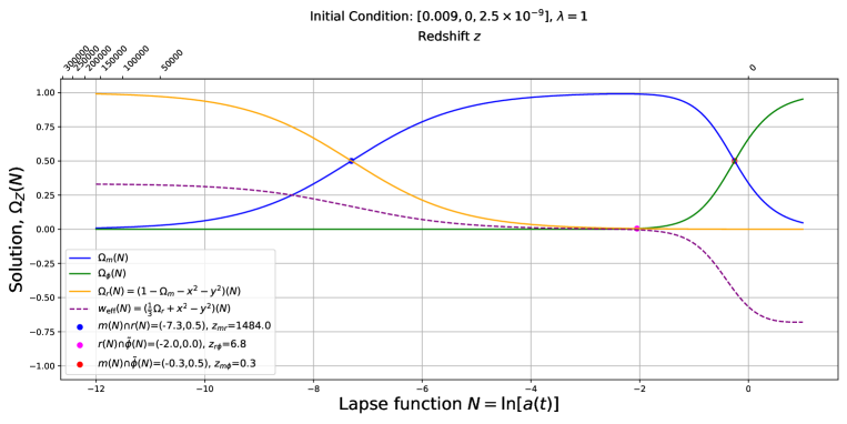
Figure 1: We illustrate the numerical solutions of the model of $\phi$CDM cosmology, in a representative case of the general behaviour of the system for which $\texttt{var-zero-is}=2.5\times 10^{-9}$, and $\lambda=1$. [See section 3.1]

$$\lambda = -\frac{V_{,\phi}}{\kappa V}=\text{constant\ number}\;,$$ (3.8)

$$\Gamma = \frac{VV_{,\phi\phi}}{(V_{,\phi})^{2}}=1$$ (3.9)

where $V_{,\phi\phi}$ is the 2nd derivative of the scalar potential in respect of the scalar field.

Effectively, the modified Friedman equations become :

$$m^{\prime} = -3m+m(4-m+2x^{2}-4y^{2})$$ (3.10)

$$x^{\prime} = -3x+\sqrt{\frac{3}{2}}\lambda y^{2}+\frac{1}{2}x(4-m+2x^{2}-4y^{2})$$ (3.11)

$$y^{\prime} = -\lambda\sqrt{\frac{3}{2}}yx+\frac{1}{2}y(4-m+2x^{2}-4y^{2})$$ (3.12)

where the $r=1-m-x^{2}-y^{2}$ . To find the critical points, we make the assumption that $(m^{\prime},x^{\prime},y^{\prime})=\vec{0}\;.$

We solve numerical the 3D system which describes the following variables, $(\Omega_{m},x,y)\;.$

We use the scipy.integrate.solveivp to solve the system of 3D system of differential equations. We find the following numerical solutions and we present them in the Fig. 1, for several specified conditions. We find the $\phi$CDM results are similar to the $\Lambda$CDM model, on the behaviour of the epoch evolution of the different species of the model. What changes is the gradient behaviour of dark energy as expected.

3.2 Stability analysis of 3D $\phi$CDM

We perform a dynamical analysis of the 3D system which describes the following variables, $\left\{m,x,y\right\}$. By solving the linearised 3D system and by identifying the eigenvalues of the Jacobian of the system, we find and characterise the critical points of the system. We provide the 3D points and their characterisation in table 1.

Note that when $\lambda=1$ we have that the point $O_{10}$ is stable, when $\lambda=-1$ we have that the point $O_{11}$ is stable, while when the value $\lambda$ is different than $1$, i.e. when the value is $\lambda=0\ ,or\ \pm 10$, then $O_{7}$ $(0,0,\pm 1)$ is the stable point. The determination is coming from the system of equations which are solved.

Point	$\Omega_{m}$	$\Omega_{r}$	$x$	$y$	condition	e.v. $\{\mu_{m},\mu_{x},\mu_{y}\}$	characterisation	$w_{\phi}$
$O$	$0$	$1$	$0$	$0$	N.A.	$\{1,-1,2\}$	saddle	$0$
$O_{1}$	$m$	$1-m$	$0$	$0$	$m\in(1/2,1]$	$\mu_{m}<0,\mu_{x}<0,\mu_{y}\geq 0$	saddle	$0$
$O_{2}$	$m$	$1-m$	$0$	$0$	$m\in(0,1/2]$	$\mu_{m}<0,\mu_{x}<0,\mu_{y}\geq 0$	saddle	$0$
$O_{3}$	$m$	$1-m-3\lambda^{-2}$	$\sqrt{\frac{3}{2}}\lambda^{-1}$	$\pm\sqrt{\frac{3}{2}}\lambda^{-1}$	$m\in[0,1]$, $|\lambda|\in[1,2]$	$\mu_{m}<0,\mu_{x}<0,\mu_{y}\geq 0$	saddle	$0$
$O_{4}$	$m$	$1-m-3\lambda^{-2}$	$\sqrt{\frac{3}{2}}\lambda^{-1}$	$\pm\sqrt{\frac{3}{2}}\lambda^{-1}$	$m\in[0,1]$, $|\lambda|\in[2,\infty]$	$\mu_{x}<0,\mu_{m},\mu_{y}\geq 0$	saddle	$0$
						$Im[\mu_{m}]=0$	Saddle (1 stable direction)
$O_{5}$	$m$	$1-m-3\lambda^{-2}$	$\sqrt{\frac{3}{2}}\lambda^{-1}$	$\pm\sqrt{\frac{3}{2}}\lambda^{-1}$	$m\in[0,1]$, $|\lambda|\in[0,1]$	$Re[\mu_{m}],Im[\mu_{x}]<0$	(Spiral $2-$counterclockwise)	$0$
						$Re[\mu_{x}],Re[\mu_{y}],Im[\mu_{y}]\geq 0$	($3-$clockwise)
						$Im[\mu_{m}]=0$	Saddle (1 stable direction)
$O_{6}$	$m$	$-m$	$\pm\frac{1}{\sqrt{2}}$	$\frac{1}{\sqrt{2}}$	$m\in[0,1]$, $|\lambda|=\frac{1}{\sqrt{2}}$	$Re[\mu_{m}],Im[\mu_{x}]<0$	Saddle (Spiral $2-$counterclockwise)	$0$
						$Re[\mu_{x}],Re[\mu_{y}],Im[\mu_{y}]\geq 0$	Saddle ($3-$clockwise)
$O_{7}$	$0$	$0$	$0$	$\pm 1$	$\lambda\in\mathbb{R}-\{\pm 1\}$	$\mu_{m},\mu_{x},\mu_{y}<0$	stable	$-1$
$O_{8}$	$0$	$0$	$\pm 1$	$0$	$\lambda\in(-3\sqrt{\frac{2}{3}},3\sqrt{\frac{2}{3}})-\{\pm 1\}$	$\mu_{m},\mu_{x},\mu_{y}>0$	unstable	$+1$
$O_{9}$	$0$	$0$	$\pm 1$	$0$	$\lambda\in(-\infty,-3\sqrt{\frac{2}{3}})\cup(3\sqrt{\frac{2}{3}},\infty)$	$\mu_{m},\mu_{x}>,\mu_{y}<0$	saddle	$+1$
$O_{10}$	$0$	$0$	$+\sqrt{\frac{1}{6}}$	$\pm\sqrt{\frac{5}{6}}$	$\lambda=1$	$\mu_{m},\mu_{x},\mu_{y}<0$	stable	$-\frac{2}{3}$
$O_{11}$	$0$	$0$	$-\sqrt{\frac{1}{6}}$	$\pm\sqrt{\frac{5}{6}}$	$\lambda=-1$	$\mu_{m},\mu_{x},\mu_{y}<0$	stable	$-\frac{2}{3}$

Table 1: The condition includes physical values for $m$, i.e., $m\in[0,1]$.

3.3 Phase portraits of the projections of 3D system

In this section, we describe the phase spaces of the 3D system projected to the 2D spaces, for different configurations of $\lambda$, i.e. $\lambda=\{-10,-1,0,1,10\}$. We selected these critical values, to be the representatives of the different conditions we found from the DA. Each point of the 2D diagram is related to a critical 3D point characterised in the table. These conditions are summarised in table 1. We find similar results for all these different configurations.

We categorise the critical points in 3D, using the notation, $O_{i}$, and we find points in the projected planes of 2D, using the notation:

$$O_{i}\to Z^{ab}_{s}(\chi,\upsilon)$$ (3.13)

where $i$ is the number of point; $Z$ represent the type of critical point, and it takes values $S$ for saddle, $A$ for attractor, and $R$ for repeller; the superscripts $a,b$ are the variable representing the plane of the point, and they take values, $m$ for matter, $x$ for the scalar kinetic term, and $y$ for the scalar potential term; the values in the parentheses $(\chi,\upsilon)$ take the numerical values of the coordinates of the points in the corresponding planes; the subscript $s$ takes values $0,+,-$, depending the position of the point in respect of the origin of the plane.

In this section, we present the phase spaces of the case of constant scalar potential, i.e. $\lambda=0$, while we present the results for $\lambda\neq 0$ in appendix C.3. We discuss our findings of these phase portraits in section 5. In Fig. 2, we plot the $(m,x)$-plane phase portrait, and we find the following points:

• The saddle point, $O\to S^{mx}_{0}(0,0)$, is characterised by a vanishing matter energy density ratio, vanishing scalar kinetic energy density ratio, vanishing scalar potential energy density ratio, and dominant radiation energy density ratio.

• The unstable point, $O_{8}\to R^{mx}_{+}(0,1)$, is characterised by a vanishing matter energy density ratio, positively dominant scalar kinetic energy density ratio, vanishing scalar potential energy density ratio, and vanishing radiation energy density ratio.

• The unstable point, $O_{8}\to R^{mx}_{-}(0,-1)$, is characterised by a vanishing matter energy density ratio, negatively dominant scalar kinetic energy density ratio, vanishing scalar potential energy density ratio, and vanishing radiation energy density ratio.

• The saddle point, $O_{1}\to S^{mx}_{0}(1,0)$, is characterised by a dominant matter energy density ratio, vanishing scalar kinetic energy density ratio, vanishing scalar potential energy density ratio, and vanishing radiation energy density ratio. Note that it looks like an attractor, but it is not in the $y$-direction, in 3D.

We observe that the dynamical field starts from the repellers $R^{mx}_{+}(0,1)$ and $R^{mx}_{-}(0,-1)$ and they go towards the attractor $A^{mx}_{0}(1,0)$. The fields also go towards the saddle point $S^{mx}_{0}(0,0)$, but they turn away before reaching it.

The physical picture is that we start with some high energy density ratio for the kinetic term of the $\phi[N(t)]$-field, i.e. $\dot{\phi}(t)\Leftrightarrow x^{2}=\Omega_{x^{2}}=\pm 1$, while vanishing energy density ratio for matter of the universe, i.e. $m=\Omega_{m}[N(t)]=0$, and then we move to a region where energy density ratio for the kinetic term of the $\phi[N(t)]$-field vanishes, i.e. $\dot{\phi}(t)\Leftrightarrow x^{2}=\Omega_{x^{2}}=0$, while the energy density ratio for matter of the universe becomes dominant, i.e. $m=\Omega_{m}[N(t)]=1$.

This signifies the transition from a vanishing matter energy density ratio, dominant scalar kinetic energy density ratio, vanishing scalar potential energy density ratio, and vanishing radiation energy density ratio epoch, towards a dominant matter energy density ratio, vanishing scalar kinetic energy density ratio, vanishing scalar potential energy density ratio, and vanishing radiation energy density ratio epoch.

Or in other words, this signifies the transition from a dominant scalar kinetic energy density ratio epoch, towards a dominant matter energy density ratio epoch.

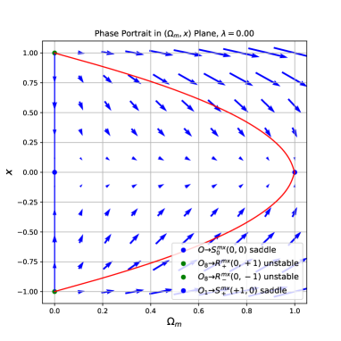
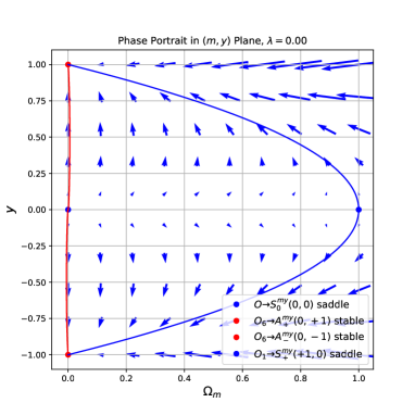
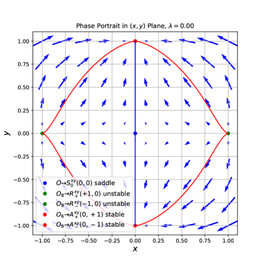
Figure 2: We illustrate the phase portrait of the 3D model, for $\lambda=0$. Left Panel: We illustrate the phase portrait of the $(m,x)$. We cannot observe the $(m,x)=(0,0)$ as a unstable initial point, but we can observe it as a saddle point. This is due to that this phase portrait is a projection of the 3D case, where both points appear. Center Panel: We illustrate the phase portrait of the $(m,y)$ Right Panel: We illustrate the phase portrait of the $(x,y)$. [See section 3.3].

In Fig. 2, we plot the $(m,y)$-plane phase portrait, and we find the following points:

• The saddle point, $O\to S^{my}_{0}(0,0)$, is characterised by a vanishing matter energy density ratio, vanishing scalar kinetic energy density ratio, vanishing scalar potential energy density ratio, and dominant radiation energy density ratio.

• The unstable point, $O_{6}\to R^{my}_{+}(1,0)$, is characterised by a positively dominant matter energy density ratio, vanishing scalar kinetic energy density ratio, vanishing scalar potential energy density ratio, and vanishing radiation energy density ratio.

• The unstable point, $O_{6}\to R^{my}_{-}(-1,0)$, is characterised by a negatively dominant matter energy density ratio, vanishing scalar kinetic energy density ratio, vanishing scalar potential energy density ratio, and vanishing radiation energy density ratio.

• The stable point, $A^{my}_{+}(0,1)$, is characterised by a vanishing matter energy density ratio, vanishing scalar kinetic energy density ratio, positively dominant scalar potential energy density ratio, and vanishing radiation energy density ratio.

• The stable point, $O_{1}\to A^{my}_{-}(0,-1)$, is characterised by a vanishing matter energy density ratio, vanishing scalar kinetic energy density ratio, negatively dominant scalar potential energy density ratio, and vanishing radiation energy density ratio.

We observe that the dynamical field starts from the repellers $R^{my}_{+}(1,0)$ and $R^{my}_{-}(-1,0)$ and they go towards the attractors $A^{my}_{+}(0,1)$ and $A^{my}_{-}(0,-1)$. The fields also go towards the saddle point $S^{my}_{0}(0,0)$, but they turn away before reaching it.

The physical picture is that we start with no matter energy density ratio $m=\Omega_{m}[N(t)]=0$ and no energy density ratio for potential term of the $V[t;N(t),\phi(N)]$-field, i.e. $V[t;N,\phi]\Leftrightarrow y^{2}=\Omega_{y^{2}}=0$, and then we move to a region where the energy density ratio for the potential term of the $V[t;N(t),\phi(N)]$-field becomes dominant, i.e. $V[t;N,\phi]\Leftrightarrow y^{2}=\Omega_{y^{2}}=\pm 1$, while we also move to a vanishing matter energy density ratio fo the kinetic term of the $m=\Omega_{m}[N(t)]=0$, while there is some increase in between.

This signifies the transition from a non dominant energy density ratio epoch for the potential energy density ratio $V[t;N(t),\phi(N)]$-field and no matter energy density ratio epoch, towards a $V[t;N(t),\phi(N)]$-field potential energy density ratio domination epoch in the far future. Note that the $V[t;N(t),\phi(N)]$-field potential energy density ratio domination epoch corresponds to a $\Lambda$ energy density ratio domination epoch in the far future.

This signifies the transition from a dominant matter energy density ratio, vanishing scalar kinetic energy density ratio, vanishing scalar potential energy density ratio, and vanishing radiation energy density ratio epoch towards a vanishing matter energy density ratio, vanishing scalar kinetic energy density ratio, dominant scalar potential energy density ratio, and vanishing radiation energy density ratio epoch.

In other words, simply, this signifies the transition from a dominant matter energy density ratio epoch towards a dominant scalar potential energy density ratio epoch.

Note that the scalar potential energy density ratio domination epoch corresponds to a $\Lambda$ energy density ratio domination epoch in the far future.

In Fig. 2, we plot the $(x,y)$-plane phase portrait, and we find the following points:

• The saddle point, $O\to S^{xy}_{0}(0,0)$, is characterised by a vanishing matter energy density ratio, vanishing scalar kinetic energy density ratio, vanishing scalar potential energy density ratio, and dominant radiation energy density ratio.

• The stable point, $O_{6}\to A^{xy}_{+}(0,1)$, is characterised by a vanishing matter energy density ratio, vanishing scalar kinetic energy density ratio, positively dominant scalar potential energy density ratio, and vanishing radiation energy density ratio.

• The stable point, $O_{6}\to A^{xy}_{-}(0,-1)$, is characterised by a vanishing matter energy density ratio, vanishing scalar kinetic energy density ratio, negatively dominant scalar potential energy density ratio, and vanishing radiation energy density ratio.

• The unstable point, $O_{8}\to R^{xy}_{+}(+1,0)$, is characterised by a vanishing matter energy density ratio, positive scalar kinetic energy density ratio, vanishing scalar potential energy density ratio, and vanishing radiation energy density ratio.

• The unstable point, $O_{8}\to R^{xy}_{-}(+1,0)$, is characterised by a vanishing matter energy density ratio, negative scalar kinetic energy density ratio, vanishing scalar potential energy density ratio, and vanishing radiation energy density ratio.

We observe that the dynamical field starts from the repellers $R^{xy}_{+}(1,0)$ and $R^{xy}_{-}(-1,0)$ and they go towards the attractors $A^{xy}_{+}(0,1)$ and $A^{xy}_{-}(0,-1)$. The fields also go towards the saddle point $S^{xy}_{0}(0,0)$, but they turn away before reaching it.

The physical picture is that we start with no energy density ratio for the kinetic term of the $\phi[N(t)]$-field, i.e. $\dot{\phi}(t)\Leftrightarrow x^{2}=\Omega_{x^{2}}=0$ and no energy density ratio for potential term of the $V[t;N(t),\phi(N)]$-field, i.e. $V[t;N,\phi]\Leftrightarrow y^{2}=\Omega_{y^{2}}=0$, and then we move to a region where the energy density ratio for the potential term of the $V[t;N(t),\phi(N)]$-field becomes dominant, i.e. $V[t;N,\phi]\Leftrightarrow y^{2}=\Omega_{y^{2}}=\pm 1$, while we also move to a vanishing energy density ratio fo the kinetic term of the $\phi[N(t)]$-field, i.e. $\dot{\phi}(t)\Leftrightarrow x^{2}=\Omega_{x^{2}}=0$.

This signifies the transition from a non dominant energy density ratio epoch for the kinetic term of the $\phi[N(t)]$-field and vanishing $V[t;N(t),\phi(N)]$-field potential energy density ratio domination epoch towards a vanishing kinetic term of the $\phi[N(t)]$-field, while we go towards a $V[t;N(t),\phi(N)]$-field potential energy density ratio domination epoch in the far future.

Note that the $V[t;N(t),\phi(N)]$-field potential energy density ratio domination epoch corresponds to a $\Lambda$ energy density ratio domination epoch in the far future.

This signifies the transition from a vanishing matter energy density ratio, dominant scalar kinetic energy density ratio, vanishing scalar potential energy density ratio, and dominant radiation energy density ratio epoch, towards a vanishing matter energy density ratio, vanishing scalar kinetic energy density ratio, dominant scalar potential energy density ratio, and vanishing radiation energy density ratio epoch.

In other words, simply, this signifies the transition from a dominant radiation energy density ratio epoch, towards a dominant scalar potential energy density ratio epoch, i.e. a $\Lambda$ energy density ratio in the far future.

Note that when $y<0$, the behaviour of the solutions corresponds to contracting universe. Note that the $y$ never diverges, since $y\propto H^{-1}$, and when $y\sim 0$, then $H$ is infinite. The case where $H\simeq 0$, does not appear in the diagrams, since that would implie $y\to\infty$, and we know by construction that $0\leq y\leq 1$. Note that the saddle point $O$, and the unstable points $O_{8}$, are either tend to the $O_{6}\to A_{+}$, $y=1$ or $O_{6}\to A_{-}$, $y=-1$, so there is no path that actually connects the point $O_{6}\to A_{+}$ and $O_{6}\to A_{-}$. So there are no heteroclinic orbits.

4 Numerical solution of $\Lambda$CDM and $\phi$CDM model comparison

We perform a comparison between the $\Lambda$CDM model (DA investigated in appendix B) and the $\phi$CDM model (DA investigated in section 3).

We identify similar numerical solutions of the two models, which is an expected results for a simple modification of gravity, such as this additional dynamical scalar fields. In agreement with current observation, we find similar behaviour for different epochs, at the level of the mean values,

• matter-radiation equality epoch redshift is the same $z^{mr}_{\Lambda\text{CDM}}=z^{mr}_{\phi\Lambda\text{CDM}}=1484$,

• radiation-dark energy equality redshift epoch is the same $z^{r\Lambda}_{\Lambda\text{CDM}}=6.5\simeq z^{r\phi}_{\phi\Lambda\text{CDM}}=6.8$,

• matter-dark energy equality epoch redshift is the same $z^{m\Lambda}_{\Lambda\text{CDM}}=z^{m\phi}_{\phi\Lambda\text{CDM}}=0.3$,

• in the far past, $t\to-\infty\Leftrightarrow N\to-\infty\Leftrightarrow z\to-\infty$, the models have a radiation domination epoch, i.e a radiation repeller.

• in the far future, $t\to+\infty\Leftrightarrow N\to-\infty\Leftrightarrow z\to+\infty$, the models have cosmological constant domination epoch, i.e. a $\Lambda$ attractor, i.e. a dark energy attractor, i.e. a de Sitter attractor.

• in the recent past, $N\to-4\Leftrightarrow z\to 50$, the models have matter domination epoch, i.e. matter saddle point.

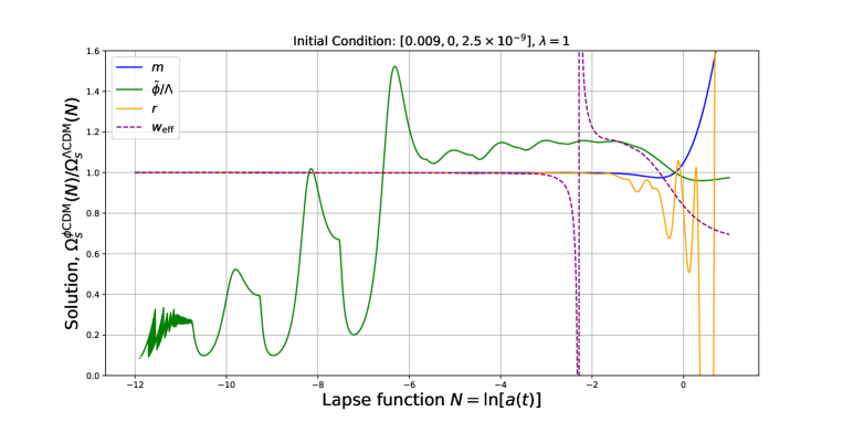
Figure 3: Comparison of numerical solutions of the energy density ratio epochs between $\Lambda$CDM and $\phi$CDM. [See section 4]

In Fig. 3, we present the ratio of energy density ratios between the two models, as a function of lapse time, $\Omega_{s}^{\phi{\rm CDM}}(N)/\Omega_{s}^{\Lambda{\rm CDM}}(N)$, for the different species, $s$. We find that

• the matter between the two models, agrees at mosts times, and in the late universe it diverges in favour of $\Lambda$CDM for $N\in[-2,-0.2]$; while for $N\in[-0.2,1]$, it diverges in favour of $\phi$CDM.

• the radiation between the two models, agrees at mosts times, and in the late universe it diverges in favour of $\Lambda$CDM for $N\in[-4,-1.6]$; while for $N\in[-1.6,-0.2]$, it diverges a lot in favour of $\Lambda$CDM, but there are huge oscillations of the ratio.

• the dark energy the constant and the dynamical between the two models, does not agree at mosts times, and in the early mid it diverges a lot in favour of $\Lambda$CDM for $N\in[-12,-6.5]$; while in the late universe for $N\in[-6.5,-0.2]$, it diverges 20% in favour of $\phi$CDM. Note that there are huge oscillations of the ratio in the late universe. In the late universe, for $N\in[-0.2,1]$, it diverges again in favour of $\Lambda$CDM.

• the equation of state between the two models, agrees at mosts times, and in the late universe it has a huge double spike, in which it diverges in favour of $\Lambda$CDM for $N\in[-4,-2.5]$; while for $N\in[-2.5,-1]$, it diverges in favour of $\phi$CDM. Note that after for $N\in[-0.5,1]$; it diverges in favour of $\Lambda$CDM.

Note that the huge spikes and oscillations are due to dividing values which are close to 0, rendering these differences are minor. While the oscillations for the dark energy models, are significant and apparent at 20%.

5 Phase portraits of $\Lambda$CDM and $\phi$CDM model comparison

Both models have the following critical points:

• the models have a radiation domination epoch, i.e a radiation repeller.

• the models have cosmological constant domination epoch, i.e. a $\Lambda$ attractor, i.e. a de Sitter attractor.

• the models have matter domination epoch, i.e. matter saddle point.

The $\Lambda$CDM model has the following transitions:

• From a radiation domination epoch to a matter domination epoch to a dark energy/cosmological constant domination epoch.

The $\phi$CDM model has the following transitions:

• for constant exponential scalar potential, $\lambda=0$, has the the following transitions:

  • transition from a dominant radiation energy density ratio epoch, towards a dominant scalar potential energy density ratio epoch, i.e. a $\Lambda$ energy density ratio in the far future, in the kinetic-potential-scalar plane $(r\to y\ \text{ or }\Lambda)$.

  • transition from a dominant matter energy density ratio epoch towards a dominant scalar potential energy density ratio epoch, in the matter-potential-scalar plane $(m\to y\ \text{ or }\Lambda)$ .

  • transition from a dominant scalar kinetic energy density ratio epoch, towards a dominant matter energy density ratio epoch, in the matter-kinetic-scalar plane $(x\to m)$.

  • transition from a dominant scalar kinetic energy density ratio epoch towards a dominant scalar kinetic energy density ratio epoch, in the kinetic-potential-scalar plane $(x\to x\text{ or }\Lambda)$.

• for low decreasing/increasing exponential scalar potential, $\lambda=\pm 1$, has the the following transitions:

  • transition from a dominant scalar kinetic energy density ratio epoch, towards a dominant matter energy density ratio epoch., in the matter-kinetic-scalar plane $(x\to m)$.

  • transition from a dominant radiation energy density ratio epoch, towards a dominant scalar potential energy density ratio epoch, in the matter-potential-scalar plane $(r\to y\ \text{ or }\Lambda)$.

  • transition from a dominant scalar kinetic energy density ratio epoch towards a dominant scalar potential energy density ratio epoch, in the kinetic-potential-scalar plane $(x\to y\ \text{ or }\Lambda)$.

• for high decreasing/increasing exponential scalar potential, $\lambda=\pm 10$, has the the following transitions:

  • transition from a dominant scalar kinetic energy density ratio epoch, towards a dominant matter energy density ratio epoch., in the matter-kinetic-scalar plane $(x\to m)$.

  • transition from a dominant radiation energy density ratio epoch, towards a dominant scalar potential energy density ratio epoch, in the matter-potential-scalar plane $(r\to y\ \text{ or }\Lambda)$.

  • transition from a negatively dominant scalar kinetic energy density ratio epoch towards a positively dominant kinetic scalar energy density ratio epoch, in the kinetic-potential-scalar plane $(x\to x)$.

Note that we have also the same transition for the matter-kinetic-scalar plane, and for all exponential scalar potentials, $\lambda=\{-10,-1,0,1,10\}$, we have :

• transition from a dominant scalar kinetic energy density ratio epoch, towards a dominant matter energy density ratio epoch., in the matter-kinetic-scalar plane $(x\to m)$.

Note that we have also the same transition for the matter-potential-scalar plane, and for all exponential scalar potentials, $\lambda=\{-10,-1,0,1,10\}$, we have :

• transition from a dominant radiation energy density ratio epoch, towards a dominant scalar potential energy density ratio epoch, in the matter-potential-scalar plane $(r\to y\ \text{ or }\Lambda)$.

In particular for the case $\lambda=-10$, for the matter-potential-scalar plane, we get:

• transition from a dominant radiation energy density ratio epoch and a low dominant matter energy density ratio and high dominant radiation energy density ratio epoch, towards a dominant scalar potential energy density ratio epoch, in the matter-potential-scalar plane $(m,r\to y\ \text{ or }\Lambda)$.

Note that in the we have also the same transition for the kinetic-potential-scalar plane, and for constant and low decreasing/increasing exponential scalar potential, $\lambda=\{-1,0,1\}$, we have :

• transition from a dominant scalar kinetic energy density ratio epoch towards a dominant potential scalar energy density ratio epoch, in the kinetic-potential-scalar plane $(x\to y\ \text{ or }\Lambda)$.

Note that in the we have also the same transition for the kinetic-potential-scalar plane, and for high decreasing exponential scalar potential, $\lambda=\pm 10$, we have :

• transition from a negatively dominant scalar kinetic energy density ratio epoch towards a positively dominant potential kinetic energy density ratio epoch, in the kinetic-potential-scalar plane $(x\to x)$.

6 Conclusions and discussion

In summary in this work we study the $\phi$CDM model with the standard $\Lambda$CDM model through the scope of dynamical analysis. The $\phi$CDM model is more complete than the one that we found in the literature, since we take into account all the so far discovered epochs, radiation, matter, and dark energy epochs. In contrast in the literature there is no study including the radiation epoch for this model.

We find that both models have the following critical points: a radiation domination epoch, i.e a radiation repeller; cosmological constant domination epoch, i.e. a $\Lambda$ attractor, i.e. a de Sitter attractor; and a matter domination epoch, i.e. matter saddle point.

The $\Lambda$CDM model has the transition from a radiation domination epoch to a matter domination epoch to a dark energy/cosmological constant domination epoch.

The $\phi$CDM model has the previous transition as well as several new transition that have not been discussed in the literature. In particular we find the main new transitions: transition from a dominant radiation energy density ratio epoch, towards a dominant scalar potential energy density ratio epoch, i.e. a $\Lambda$ energy density ratio in the far future, in the kinetic-potential-scalar plane $(r\to y\ \text{ or }\Lambda)$; transition from a dominant matter energy density ratio epoch towards a dominant scalar potential energy density ratio epoch, in the matter-potential-scalar plane $(m\to y\ \text{ or }\Lambda)$; transition from a dominant scalar kinetic energy density ratio epoch, towards a dominant matter energy density ratio epoch, in the matter-kinetic-scalar plane $(x\to m)$; and finally the exotic transition from a dominant radiation energy density ratio epoch and a low dominant matter energy density ratio and high dominant radiation energy density ratio epoch, towards a dominant scalar potential energy density ratio epoch, in the matter-potential-scalar plane $(m,r\to y\ \text{ or }\Lambda)$.

Future work includes exploring the dynamics of several potentials, and the dynamics of more interesting and sophisticated systems such as the $f(R)$, Horndeski, non-Riemannian cosmologies, cosmologies at perturbation levels [28], compactified dynamical system in cosmology, and functor of actions theories [13, 14].

Appendix A Triples in different epochs

In table 2, we present the different epochs of time triplet corresponding to the different energy density ratio species equivalences.

Epoch	lapse function, $N(t)$	redshift, $z(t)$	scale factor, $a(t)$
today, $0$	0	0	1
matter-Dark energy, $m\Lambda$	-0.282	0.326	0.753
radiation-Dark energy, $r\Lambda$	-2.04	7.69	0.130
decoupling	-7.01	1089	$9\times 10^{-4}$
recombination	-7.01	1100	$9\times 10^{-4}$
matter-radiation, $mr$	-7.31	1500	$7\times 10^{-4}$
initial, $i$	-12	$2\times 10^{5}$	$6\times 10^{-6}$

Table 2: Classification of time triplet epoch according to species energy density ratio.

Appendix B Dynamical system analysis on $\Lambda$CDM

Following [8], we model the $\Lambda$CDM-Cosmology, and we apply the dynamical system analysis as follows.

B.1 The $\Lambda$CDM model

We know that assuming a non-curved, flat FLRW metric, and standard General Relativity Gravity, namely, $R$-Gravity, we obtain the following cosmological scenario, using a cosmological constant and cold dark matter, and assuming the least action principle, the $\Lambda$CDM-Cosmology is governed by the background Einstein Field Equations equations, $G_{\mu\nu}=\kappa^{2}T_{\mu\nu}\;,$ where $\kappa^{2}=\frac{8\pi G_{\rm N}}{c^{4}}$. These result to Friedman equations which have the species matter, radiation, and cosmological constant, $\Lambda$. and we also use the continuity equation ${T^{\mu\nu}}_{;\mu}=0\;$ . For each different energy density species we have a different equation of state: $\{w_{m},w_{r},w_{\Lambda}\}=\{0,1/3,-1\}\;,$ which corresponds to a different energy density species continuity equations.

B.2 Defining the dimensionless variables for $\Lambda$CDM

To apply the dynamical analysis, we need to simplify mathematically the problem, and we define the following dimensionless variables

$$x(t) = \Omega_{m}(t)=\frac{\kappa^{2}\rho_{\rm m}(t)}{3H^{2}(t)},\quad y(t)=\Omega_{r}(t)=\frac{\kappa^{2}\rho_{\rm r}(t)}{3H^{2}(t)}$$ (B.1)

$$z(t) = \Omega_{\Lambda}(t)=\frac{\kappa^{2}\rho_{\rm\Lambda}}{3H^{2}(t)}\equiv\frac{\Lambda}{3H^{2}(t)}\;.$$ (B.2)

Using the previous definitions, we write the 3D set of differential equations simply

$$x^{\prime} = x(-3+3x+4y)$$ (B.3)

$$y^{\prime} = y(-4+3x+4y)$$ (B.4)

$$z^{\prime} = +(1-x-y)(3x+4y)$$ (B.5)

where we integrate in the previous set of equations; the 1st Friedmann equation for the model: $z=1-x-y\;.$

According to these definition, the effective equation of state, for this model, is given by

$$w_{\rm eff}=\sum_{s\in\left\{m,r,\Lambda\right\}}w_{s}(t)\Omega_{s}(t)=\frac{1}{3}y(t)-z(t)\;.$$ (B.6)

B.3 $\Lambda$CDM model: system in 2D, 3D projected to 2D and 3D approaches

We solve the system analytically and numerically in 2D, 3D projected to 2D and in 3D and we find similar results for the epoch evolution of the different species in our $\Lambda$CDM model. We also apply the DA to the system and we obtain similar phase portraits and results, in 2D in 3D projected to 2D and in 3D. The 3D projected to 2D and the 3D cases, are not customary done in the literature, however we find that they are equivalent. In this work, we provide 3D equivalent approach. We use the solutions and the DA for the 3D model.

B.4 Dynamical analysis of the 3D set of differential equations of $\Lambda$CDM model

We solve the system of simultaneous differential equations of $(x,y,z)$ as a function of lapse function $N$, described by equations B.3-B.5, numerically, using the ipython library scipy.integrate.solveivp. The selection of the 3D system is explained in appendix B.3

We use different initial conditions. However, the most physical one, is the one where

$$\left\{x(N_{i}),y(N_{i}),z(N_{i})\right\}=\{0.01,0.99,0\}\;.$$ (B.7)

This is the most physical one, since the sum of all these functions should be equal to 1 at all times, and also because we have good evidence that initial the universe was mostly field with radiation, and some dark energy, and some matter energy densities, although the latter two should be vanishing. Note that the range for the lapse function is $\Delta N=[-1,1]$.

We find that the system with initial conditions for which initial dark energy density ratio, is higher than or comparable with the initial total matter density ratio, then the total matter density ratio, is not allowed by the system to evolve, and it is quickly suppressed. While in the case for which initial dark energy density ratio, is lower than the initial total matter density ratio, then the total matter density ratio, is allowed by the system to evolve better, and it is quickly increases to describe the matter dominated epoch, as we know so far by observations and previous theories. We find the numerical solutions of the 3D system.

B.4.1 Stability analysis on 3D system of $\Lambda$CDM

To analyze the stability of the critical points, we need to compute the Jacobian matrix of the system. The Jacobian matrix $J$ is given by the matrix of partial derivatives of the right-hand sides of the system with respect to the variables $x$, $y$, and $z$. We find its corresponding eigenvalues to characterise the critical points.

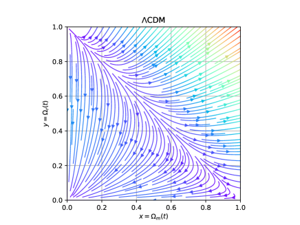
Figure 4: We illustrate the phase portrait of $\Lambda$CDM cosmology. [See appendix B.4.1]

The summary of stability is the following:

- The critical point $(x,y)=(0,0)$ is a stable point. The eigenvalues of this matrix are $-3$, $-4$, and $0$. Since two eigenvalues are negative and one is zero, this critical point is a stable point (Attractor).

- The critical point $(x,y)=(0,1)$ is unstable. The eigenvalues of this matrix are $1$, $4$, and $0$. Since two eigenvalues are positive and one is zero, this critical point is unstable (repelling).

- The critical point $(x,y)=(1,0)$ is a saddle point. The eigenvalues of this matrix are $6$, $-1$, and $0$. Since one eigenvalue is positive and one is negative, this critical point is also a saddle point.

This provides insight into the dynamics of your system near these points.

We present the results in Fig. 4.

We find that the universe starts with a radiation energy density ratio domination epoch at the unstable repeller point $R^{xy}(0,1)=R^{mr}(0,1)$, transits to a matter energy density ratio domination epoch, at the saddle point, $R^{xy}(1,0)=R^{mr}(1,0)$, and it is attracted in the far future to the stable attractor point, $R^{xy}(0,0)=R^{mr}(0,0)$, i.e it results to a dark energy density ratio domination epoch.

In simple terms we conclude the following.

We find that the universe starts with a radiation energy density ratio domination epoch, then it transits to a matter energy density ratio domination epoch and it is attracted, in the far future, to a dark energy density ratio domination epoch.

Appendix C Details of the $\phi$CDM dynamical analysis

Below, we provide all the necessary details of the $\phi$CDM dynamical analysis.

C.1 The $\phi$CDM action

The $\phi$CDM action is written as

$$S_{\phi\text{CDM}} = c^{3}\int d(ct)d^{3}x\sqrt{-g}\left[\frac{R}{16\pi G_{\rm N}}+\mathcal{L}_{\rm mr}+\mathcal{L}_{\phi}\right]$$ (C.1)

$$\mathcal{L}_{\phi} = -\frac{1}{2}g_{\mu\nu}\partial^{\mu}\phi\partial^{\nu}\phi+V[t,\Lambda;\phi(t)]$$ (C.2)

where $c$ is the sped of light, $G_{\rm N}$ is the Newton constant, $g$ is the determinant of the metric, $g_{\mu\nu}$, $R=R[g]$ is the ricci scalar, $\Lambda$ is the cosmological constant, $\mathcal{L}_{\rm mr}[g,\psi_{mr}]$ is the lagrangian describing matter and radiation field, $\psi_{\rm mr}$, $\phi$ is a scalar dynamical field, with a kinetic term, described by partial derivatives, and $V[t,\Lambda;\phi(t)]$ is its potential. Assuming the least actionic principle, varying the aforementioned action, we are lead to the following equations of motion of the system.

C.2 The cosmological constant, $\Lambda$, in $\phi$CDM

In the standard cosmological model, $\Lambda$ cosmological constant describe dark energy. In our case, the $\phi$CDM model, now we have a dynamical scalar field which describes dark energy, however the cosmological constant is still inherent in our model, through the following consideration.

The choice of the potential of this scalar field is

$$V(\phi)=V[t,\Lambda;\phi(t)]=V_{0}(\Lambda)e^{-\kappa\lambda\phi(t)}$$

where $V_{0}(\Lambda)$ is the normailsation constant of the potential.

To retrieve the $\Lambda$CDM model from $\phi$CDM model, we need the condition:

$$V_{0}(\Lambda)=-\frac{1}{16\pi G_{\rm N}}2\Lambda\hskip 28.45274pt\text{and}\hskip 28.45274pt\phi(t)=0$$

In that case the potential becomes

$$V(\phi)=-\frac{1}{16\pi G_{\rm N}}2\Lambda$$

and the action model

$$S_{\phi\text{CDM}}=c^{3}\int d(ct)d^{3}x\sqrt{-g}\left[\frac{R}{16\pi G_{\rm N}}+\mathcal{L}_{\rm mr}+\mathcal{L}_{\phi}\right]$$ (C.3)

becomes

$$S_{\Lambda\text{CDM}}=c^{3}\int d(ct)d^{3}x\sqrt{-g}\left[\frac{R}{16\pi G_{\rm N}}+\mathcal{L}_{\rm mr}-\frac{2\Lambda}{16\pi G_{\rm N}}\right]\>.$$ (C.4)

C.3 Phase space portraits of $\phi$CDM model, $\lambda\neq 0$

In this section, we present the phase space portraits of $\phi$CDM model, $\lambda\neq 0$, for an increasing ($\lambda<0$) or decreasing ($\lambda>0$) exponential scalar potential.

C.3.1 Phase portrait in $(m,x,y)$ planes, Case: low decreasing exponential scalar potential $\lambda\in[1,2]$

In Fig. 5, we plot the $(m,x)$-plane phase portrait for low decreasing exponential scalar potential, $\lambda=1$, and we find the same results as in the cases $\lambda=0$.

In Fig. 5, we plot the $(m,x)$-plane phase portrait, and we find the following points:

• The saddle point, $O\to S^{mx}_{0}(0,0)$, is characterised by a vanishing matter energy density ratio, vanishing scalar kinetic energy density ratio, vanishing scalar potential energy density ratio, and dominant radiation energy density ratio.

• The unstable point, $O_{8}\to R^{mx}_{+}(0,1)$, is characterised by a vanishing matter energy density ratio, positively dominant scalar kinetic energy density ratio, vanishing scalar potential energy density ratio, and vanishing radiation energy density ratio.

• The unstable point, $O_{8}\to R^{mx}_{-}(0,-1)$, is characterised by a vanishing matter energy density ratio, negatively dominant scalar kinetic energy density ratio, vanishing scalar potential energy density ratio, and vanishing radiation energy density ratio.

• The saddle point, $O_{1}\to S^{mx}_{+}(1,0)$, is characterised by a dominant matter energy density ratio, vanishing scalar kinetic energy density ratio, vanishing scalar potential energy density ratio, and vanishing radiation energy density ratio. Note that this is a saddle point in 3D.

We observe that the dynamical field starts from the repellers $R^{mx}_{+}(0,1)$ and $R^{mx}_{-}(0,-1)$ and they go towards the saddle $S^{mx}_{+}(1,0)$. The fields also go towards the saddle point $S^{mx}_{0}(0,0)$, but they turn away before reaching it.

The physical picture is that we start with some high energy density ratio for the kinetic term of the $\phi[N(t)]$-field, i.e. $\dot{\phi}(t)\Leftrightarrow x^{2}=\Omega_{x^{2}}=\pm 1$, while vanishing energy density ratio for matter of the universe, i.e. $m=\Omega_{m}[N(t)]=0$, and then we move to a region where energy density ratio for the kinetic term of the $\phi[N(t)]$-field vanishes, i.e. $\dot{\phi}(t)\Leftrightarrow x^{2}=\Omega_{x^{2}}=0$, while the energy density ratio for matter of the universe becomes dominant, i.e. $m=\Omega_{m}[N(t)]=1$.

This signifies the transition from a vanishing matter energy density ratio, dominant scalar kinetic energy density ratio, vanishing scalar potential energy density ratio, and vanishing radiation energy density ratio epoch, towards a dominant matter energy density ratio, vanishing scalar kinetic energy density ratio, vanishing scalar potential energy density ratio, and vanishing radiation energy density ratio epoch.

In other words, simply, this signifies the transition from a dominant scalar kinetic energy density ratio epoch, towards a dominant matter energy density ratio epoch.

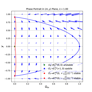
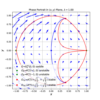
Figure 5: We illustrate the phase portrait of the 3D model, for $\lambda=1$, which represents the $|\lambda|\in[1,2]$. Left Panel: We illustrate the phase portrait of the $(m,x)$. Center Panel: We illustrate the phase portrait of the $(m,y)$ Right Panel: We illustrate the phase portrait of the $(x,y)$. [See sections C.3.1, C.3.2, and C.3.3.

C.3.2 Phase portrait in $(m,y)$-plane, Case: low decreasing exponential scalar potential $\lambda\in[1,2]$

In Fig. 5, we find the results for the $(m,y)$-plane phase portrait for low decreasing exponential scalar potential, $\lambda=1$, which are the similar as the results for $\lambda=0$.

In particular, in Fig. 5, we plot the $(m,y)$-plane phase portrait, and we find the following points:

• The unstable point, $O_{8}\to R^{my}_{0}(0,0)$, is characterised by a vanishing matter energy density ratio, vanishing scalar kinetic energy density ratio, vanishing scalar potential energy density ratio, and dominant radiation energy density ratio.

• The stable point, $O_{1}\to A^{my}_{+}(0,1)$, is characterised by a vanishing matter energy density ratio, vanishing scalar kinetic energy density ratio, positively dominant scalar potential energy density ratio, and vanishing radiation energy density ratio.

• The stable point, $O_{7}\to A^{my}_{-}(0,-1)$, is characterised by a vanishing matter energy density ratio, vanishing scalar kinetic energy density ratio, negatively dominant scalar potential energy density ratio, and vanishing radiation energy density ratio.

• The saddle point, $O_{7}\to S^{my}_{0}(1,0)$, is characterised by a dominant matter energy density ratio, vanishing scalar kinetic energy density ratio, vanishing scalar potential energy density ratio, and vanishing radiation energy density ratio.

We observe that the dynamical field starts from the repellers $R^{my}_{+}(1,0)$ and $R^{my}_{-}(-1,0)$ and they go towards the attractors $A^{my}_{+}(0,1)$ and $A^{my}_{-}(0,-1)$. The fields also go towards the saddle point $S^{my}_{0}(1,0)$, but they turn away before reaching it.

The physical picture is that we start with no matter energy density ratio $m=\Omega_{m}[N(t)]=0$ and no energy density ratio for potential term of the $V[t;N(t),\phi(N)]$-field, i.e. $V[t;N,\phi]\Leftrightarrow y^{2}=\Omega_{y^{2}}=0$, and then we move to a region where the energy density ratio for the potential term of the $V[t;N(t),\phi(N)]$-field becomes dominant, i.e. $V[t;N,\phi]\Leftrightarrow y^{2}=\Omega_{y^{2}}=\pm 1$, while we also move to a vanishing matter energy density ratio fo the kinetic term of the $m=\Omega_{m}[N(t)]=0$, while there is some increase in between.

This signifies the transition from a vanishing matter energy density ratio, vanishing scalar kinetic energy density ratio, vanishing scalar potential energy density ratio, and dominant radiation energy density ratio epoch, towards a vanishing matter energy density ratio, vanishing scalar kinetic energy density ratio, dominant scalar potential energy density ratio, and vanishing radiation energy density ratio epoch.

In other words, simply, this signifies the transition from a dominant radiation energy density ratio epoch, towards a dominant scalar potential energy density ratio epoch.

Note that the dominant scalar potential energy density ratio epoch corresponds to a $\Lambda$ energy density ratio domination epoch in the far future.

C.3.3 Phase portrait in $(x,y)$-plane, Case: low decreasing exponential scalar potential $\lambda\in[+1,+2]$

In Fig. 5, we plot the $(x,y)$-plane phase portrait, and we find the following points:

• The saddle point, $O\to S^{xy}_{+}(0,0)$, is characterised by a vanishing matter energy density ratio, vanishing scalar kinetic energy density ratio, vanishing scalar potential energy density ratio, and dominant radiation energy density ratio.

• The unstable point, $O_{8}\to R^{xy}_{+}(1,0)$, is characterised by a vanishing matter energy density ratio, positively dominant scalar kinetic energy density ratio, vanishing scalar potential energy density ratio, and vanishing radiation energy density ratio.

• The unstable point, $O_{8}\to R^{xy}_{-}(-1,0)$, is characterised by a vanishing matter energy density ratio, negatively dominant scalar kinetic energy density ratio, vanishing scalar potential energy density ratio, and vanishing radiation energy density ratio.

• The stable point, $O_{10}\to A^{xy}_{+}(\sqrt{\frac{1}{6}},\sqrt{\frac{5}{6}})$, is characterised by a vanishing matter energy density ratio, positively low dominant scalar kinetic energy density ratio, positively high dominant scalar potential energy density ratio, and vanishing radiation energy density ratio.

• The stable point, $O_{10}\to A^{xy}_{-}(\sqrt{\frac{1}{6}},-\sqrt{\frac{5}{6}})$, is characterised by a vanishing matter energy density ratio, positively low dominant scalar kinetic energy density ratio, negatively high dominant scalar potential energy density ratio, and vanishing radiation energy density ratio.

We observe that the dynamical field starts from the repellers $R^{xy}_{+}(1,0)$ and $R^{xy}_{-}(-1,0)$ and they go towards the attractors $A^{xy}_{+}(\sqrt{\frac{1}{6}},\sqrt{\frac{5}{6}})$ and $A^{xy}_{-}(\sqrt{\frac{1}{6}},-\sqrt{\frac{5}{6}})$. The fields also go towards the saddle point $S^{xy}_{+}(1,0)$, but they turn away before reaching it.

The physical picture is that we start with no energy density ratio for the kinetic term of the $\phi[N(t)]$-field, i.e. $\dot{\phi}(t)\Leftrightarrow x^{2}=\Omega_{x^{2}}=0$ and no energy density ratio for potential term of the $V[t;N(t),\phi(N)]$-field, i.e. $V[t;N,\phi]\Leftrightarrow y^{2}=\Omega_{y^{2}}=0$, and then we move to a region where the energy density ratio for the potential term of the $V[t;N(t),\phi(N)]$-field becomes dominant, i.e. $V[t;N,\phi]\Leftrightarrow y^{2}=\Omega_{y^{2}}=\pm 1$, while we also move to a vanishing energy density ratio fo the kinetic term of the $\phi[N(t)]$-field, i.e. $\dot{\phi}(t)\Leftrightarrow x^{2}=\Omega_{x^{2}}=0$.

This signifies the transition from a non dominant energy density ratio epoch for the kinetic term of the $\phi[N(t)]$-field and vanishing $V[t;N(t),\phi(N)]$-field potential energy density ratio domination epoch towards a vanishing kinetic term of the $\phi[N(t)]$-field, while we go towards a $V[t;N(t),\phi(N)]$-field potential energy density ratio domination epoch in the far future. Note that the $V[t;N(t),\phi(N)]$-field potential energy density ratio domination epoch corresponds to a $\Lambda$ energy density ratio domination epoch in the far future.

This signifies the transition from a vanishing matter energy density ratio, dominant scalar kinetic energy density ratio, vanishing scalar potential energy density ratio, and vanishing radiation energy density ratio epoch towards a vanishing matter energy density ratio, positively low dominant scalar kinetic energy density ratio, high dominant scalar potential energy density ratio, and vanishing radiation energy density ratio epoch.

In other words, simply, this signifies the transition from a dominant scalar kinetic energy density ratio epoch towards a positively low dominant scalar kinetic energy density ratio, high dominant scalar potential energy density ratio epoch.

Note that the dominant scalar potential energy density ratio epoch corresponds to a $\Lambda$ energy density ratio domination epoch in the far future.

C.3.4 Phase portrait in $(m,x)$-plane, Case: low increasing exponential scalar potential $\lambda\in[-1,-2]$

In Fig. 6, we plot the $(m,x)$-plane phase portrait for low decreasing exponential scalar potential $\lambda=-1$, and we find the same results as in the cases $\lambda=0$ or $1$.

In particular, in Fig. 6, we plot the $(m,x)$-plane phase portrait, and we find the following points:

• The saddle point, $O\to S^{mx}_{0}(0,0)$, is characterised by a vanishing matter energy density ratio, vanishing scalar kinetic energy density ratio, vanishing scalar potential energy density ratio, and dominant radiation energy density ratio.

• The unstable point, $O_{8}\to R^{mx}_{+}(0,1)$, is characterised by a vanishing matter energy density ratio, positively dominant scalar kinetic energy density ratio, vanishing scalar potential energy density ratio, and vanishing radiation energy density ratio.

• The unstable point, $O_{8}\to R^{mx}_{-}(0,-1)$, is characterised by a vanishing matter energy density ratio, negatively dominant scalar kinetic energy density ratio, vanishing scalar potential energy density ratio, and vanishing radiation energy density ratio.

• The saddle point, $O_{1}\to S^{mx}_{+}(1,0)$, is characterised by a dominant matter energy density ratio, vanishing scalar kinetic energy density ratio, vanishing scalar potential energy density ratio, and vanishing radiation energy density ratio. Note that this is a saddle point in 3D.

We observe that the dynamical field starts from the repellers $R^{mx}_{+}(0,1)$ and $R^{mx}_{-}(0,-1)$ and they go towards the saddle $S^{mx}_{+}(1,0)$. The fields also go towards the saddle point $S^{mx}_{0}(0,0)$, but they turn away before reaching it.

The physical picture is that we start with some high energy density ratio for the kinetic term of the $\phi[N(t)]$-field, i.e. $\dot{\phi}(t)\Leftrightarrow x^{2}=\Omega_{x^{2}}=\pm 1$, while vanishing energy density ratio for matter of the universe, i.e. $m=\Omega_{m}[N(t)]=0$, and then we move to a region where energy density ratio for the kinetic term of the $\phi[N(t)]$-field vanishes, i.e. $\dot{\phi}(t)\Leftrightarrow x^{2}=\Omega_{x^{2}}=0$, while the energy density ratio for matter of the universe becomes dominant, i.e. $m=\Omega_{m}[N(t)]=1$.

This signifies the transition from a vanishing matter energy density ratio, dominant scalar kinetic energy density ratio, vanishing scalar potential energy density ratio, and vanishing radiation energy density ratio epoch, towards a dominant matter energy density ratio, vanishing scalar kinetic energy density ratio, vanishing scalar potential energy density ratio, and vanishing radiation energy density ratio epoch.

In other words, simply, this signifies the transition from a dominant scalar kinetic energy density ratio epoch, towards a dominant matter energy density ratio epoch, in the matter-kinetic-scalar plane.

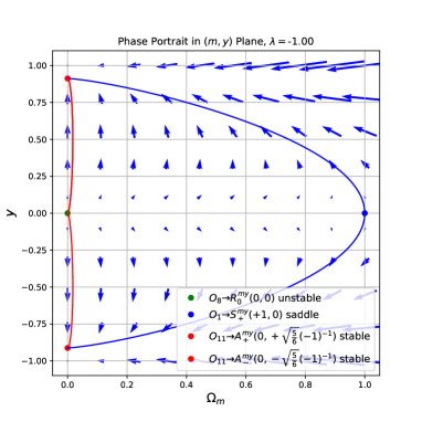
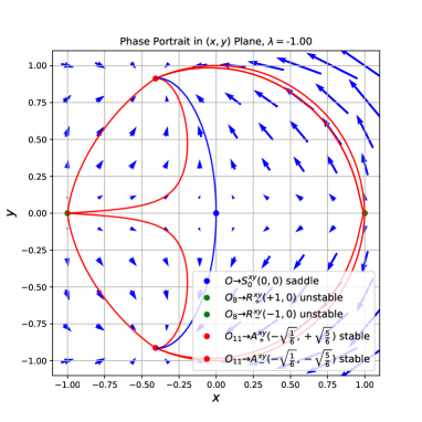
Figure 6: We illustrate the phase portrait of the 3D model, for $\lambda=-1$, which represents the $\lambda\in[-1,-2]$. Left Panel: We illustrate the phase portrait of the $(m,x)$. Center Panel: We illustrate the phase portrait of the $(m,y)$ Right Panel: We illustrate the phase portrait of the $(x,y)$. [See sections C.3.4, C.3.5, and C.3.6].

C.3.5 Phase portrait in $(m,y)$-plane, Case: low increasing exponential scalar potential $\lambda\in[-1,-2]$

In Fig. 6, we find the results for the $(m,y)$-plane phase portrait for low increasing exponential scalar potential $\lambda=-1$, which are the same as the results for $\lambda=\{1\}$.

In particular, in Fig. 6, we plot the $(m,y)$-plane phase portrait, and we find the following points:

• The unstable point, $O_{8}\to R^{my}_{0}(0,0)$, is characterised by a vanishing matter energy density ratio, vanishing scalar kinetic energy density ratio, vanishing scalar potential energy density ratio, and dominant radiation energy density ratio.

• The stable point, $O_{11}\to A^{my}_{+}(0,1)$, is characterised by a vanishing matter energy density ratio, vanishing scalar kinetic energy density ratio, positively dominant scalar potential energy density ratio, and vanishing radiation energy density ratio.

• The stable point, $O_{11}\to A^{my}_{-}(0,-1)$, is characterised by a vanishing matter energy density ratio, vanishing scalar kinetic energy density ratio, negatively dominant scalar potential energy density ratio, and vanishing radiation energy density ratio.

• The saddle point, $O_{8}\to S^{my}_{+}(1,0)$, is characterised by a dominant matter energy density ratio, vanishing scalar kinetic energy density ratio, vanishing scalar potential energy density ratio, and vanishing radiation energy density ratio.

We observe that the dynamical field starts from the repellers $R^{my}_{+}(1,0)$ and $R^{my}_{-}(-1,0)$ and they go towards the attractors $A^{my}_{+}(0,1)$ and $A^{my}_{-}(0,-1)$. The fields also go towards the saddle point $S^{my}_{+}(1,0)$, but they turn away before reaching it.

The physical picture is that we start with no matter energy density ratio $m=\Omega_{m}[N(t)]=0$ and no energy density ratio for potential term of the $V[t;N(t),\phi(N)]$-field, i.e. $V[t;N,\phi]\Leftrightarrow y^{2}=\Omega_{y^{2}}=0$, and then we move to a region where the energy density ratio for the potential term of the $V[t;N(t),\phi(N)]$-field becomes dominant, i.e. $V[t;N,\phi]\Leftrightarrow y^{2}=\Omega_{y^{2}}=\pm 1$, while we also move to a vanishing matter energy density ratio fo the kinetic term of the $m=\Omega_{m}[N(t)]=0$, while there is some increase in between.

This signifies the transition from a vanishing matter energy density ratio, vanishing scalar kinetic energy density ratio, vanishing scalar potential energy density ratio, and dominant radiation energy density ratio epoch, towards a vanishing matter energy density ratio, vanishing scalar kinetic energy density ratio, dominant scalar potential energy density ratio, and vanishing radiation energy density ratio epoch.

In other words, simply, this signifies the transition from a dominant radiation energy density ratio epoch, towards a dominant scalar potential energy density ratio epoch.

Note that the dominant scalar potential energy density ratio epoch corresponds to a $\Lambda$ energy density ratio domination epoch in the far future.

C.3.6 Phase portrait in $(x,y)$-plane, Case: low increasing exponential scalar potential $\lambda\in[-1,-2]$

In Fig. 6, we plot the $(x,y)$-plane phase portrait for low increasing exponential scalar potential, $\lambda=-1$, and we find similar but not the same results as in the cases $\lambda=\{0,1\}$. The difference, is that the attractors appear to negative values for energy density ratio for the kinetic term, $x$.

In particular, in Fig. 6, we plot the $(x,y)$-plane phase portrait, and we find the following points:

• The saddle point, $O\to S^{xy}_{+}(0,0)$, is characterised by a vanishing matter energy density ratio, vanishing scalar kinetic energy density ratio, vanishing scalar potential energy density ratio, and dominant radiation energy density ratio.

• The unstable point, $O_{8}\to R^{xy}_{+}(1,0)$, is characterised by a vanishing matter energy density ratio, positively dominant scalar kinetic energy density ratio, vanishing scalar potential energy density ratio, and vanishing radiation energy density ratio.

• The unstable point, $O_{8}\to R^{xy}_{-}(-1,0)$, is characterised by a vanishing matter energy density ratio, negatively dominant scalar kinetic energy density ratio, vanishing scalar potential energy density ratio, and vanishing radiation energy density ratio.

• The stable point, $O_{11}\to A^{xy}_{+}(-\sqrt{\frac{1}{6}},\sqrt{\frac{5}{6}})$, is characterised by a vanishing matter energy density ratio, negatively low dominant scalar kinetic energy density ratio, positively high dominant scalar potential energy density ratio, and vanishing radiation energy density ratio.

• The stable point, $O_{11}\to A^{xy}_{-}(-\sqrt{\frac{1}{6}},-\sqrt{\frac{5}{6}})$, is characterised by a vanishing matter energy density ratio, negatively low dominant scalar kinetic energy density ratio, negatively high dominant scalar potential energy density ratio, and vanishing radiation energy density ratio.

We observe that the dynamical field starts from the repellers $R^{xy}_{+}(1,0)$ and $R^{xy}_{-}(-1,0)$ and they go towards the attractors $A^{xy}_{+}(-\sqrt{\frac{1}{6}},\sqrt{\frac{5}{6}})$ and $A^{xy}_{-}(-\sqrt{\frac{1}{6}},-\sqrt{\frac{5}{6}})$. The fields also go towards the saddle point $S^{xy}_{+}(1,0)$, but they turn away before reaching it.

The physical picture is that we start with dominant energy density ratio for the kinetic term of the $\phi[N(t)]$-field, i.e. $\dot{\phi}(t)\Leftrightarrow x^{2}=\Omega_{x^{2}}=0$ and no energy density ratio for potential term of the $V[t;N(t),\phi(N)]$-field, i.e. $V[t;N,\phi]\Leftrightarrow y^{2}=\Omega_{y^{2}}=0$, and then we move to a region where the energy density ratio for the potential term of the $V[t;N(t),\phi(N)]$-field becomes dominant, i.e. $V[t;N,\phi]\Leftrightarrow y^{2}=\Omega_{y^{2}}=\pm 1$, while we also move to a low domination of energy density ratio fo the kinetic term of the $\phi[N(t)]$-field, i.e. $\dot{\phi}(t)\Leftrightarrow x^{2}=\Omega_{x^{2}}=0$.

This signifies the transition from a dominant energy density ratio epoch for the kinetic term of the $\phi[N(t)]$-field and vanishing $V[t;N(t),\phi(N)]$-field potential energy density ratio domination epoch towards a low domination of the kinetic term of the $\phi[N(t)]$-field, while we go towards a high domination of the $V[t;N(t),\phi(N)]$-field potential energy density ratio epoch in the far future. Note that the $V[t;N(t),\phi(N)]$-field potential energy density ratio domination epoch corresponds to a $\Lambda$ energy density ratio domination epoch in the far future.

This signifies the transition from a vanishing matter energy density ratio, dominant scalar kinetic energy density ratio, vanishing scalar potential energy density ratio, and vanishing radiation energy density ratio epoch towards a vanishing matter energy density ratio, negatively low dominant scalar kinetic energy density ratio, high dominant scalar potential energy density ratio, and vanishing radiation energy density ratio epoch.

In other words, simply, this signifies the transition from a dominant scalar kinetic energy density ratio epoch towards a negatively low dominant scalar kinetic energy density ratio, high dominant scalar potential energy density ratio epoch.

Note that the dominant scalar potential energy density ratio epoch corresponds to a $\Lambda$ energy density ratio domination epoch in the far future.

C.3.7 Phase portrait in $(m,x)$-plane, Case: high decreasing exponential scalar potential $\lambda\in[+2,+\infty)$

In Fig. 7, we plot the $(m,x)$-plane phase portrait for high decreasing exponential scalar potential, $\lambda=10$, and we find the similar results as in the cases $\lambda=\{-1,0,1\}$.

In Fig. 7, we plot the $(m,x)$-plane phase portrait, and we find the following points:

• The saddle point, $O\to S^{mx}_{0}(0,0)$, is characterised by a vanishing matter energy density ratio, vanishing scalar kinetic energy density ratio, vanishing scalar potential energy density ratio, and dominant radiation energy density ratio.

• The unstable point, $O_{8}\to R^{mx}_{+}(0,1)$, is characterised by a vanishing matter energy density ratio, positively dominant scalar kinetic energy density ratio, vanishing scalar potential energy density ratio, and vanishing radiation energy density ratio.

• The unstable point, $O_{8}\to R^{mx}_{-}(0,-1)$, is characterised by a vanishing matter energy density ratio, negatively dominant scalar kinetic energy density ratio, vanishing scalar potential energy density ratio, and vanishing radiation energy density ratio.

• The saddle point, $O_{1}\to S^{mx}_{+}(1,0)$, is characterised by a dominant matter energy density ratio, vanishing scalar kinetic energy density ratio, vanishing scalar potential energy density ratio, and vanishing radiation energy density ratio.

• The saddle point, $O_{5}\to S^{mx}_{+}(0,+\sqrt{\frac{3}{2}}(10)^{-1})$, is characterised by a vanishing matter energy density ratio, positively low dominant scalar kinetic energy density ratio, vanishing scalar potential energy density ratio, and dominant radiation energy density ratio.

• The saddle point, $O_{5}\to S^{mx}_{-}(0,-\sqrt{\frac{3}{2}}(10)^{-1})$, is characterised by a vanishing matter energy density ratio, negatively low dominant scalar kinetic energy density ratio, vanishing scalar potential energy density ratio, and dominant radiation energy density ratio.

We observe that the dynamical field starts from the repellers $R^{mx}_{+}(0,1)$ and $R^{mx}_{-}(0,-1)$ and they go towards the attractor $A^{mx}_{0}(1,0)$. The fields also go towards the saddle points $S^{mx}_{0}(0,0)$ $S^{mx}_{+}(0,+\sqrt{\frac{3}{2}}(10)^{-1})$, $S^{mx}_{-}(0,-\sqrt{\frac{3}{2}}(10)^{-1})$, but they turn away before reaching them.

The physical picture is that we start with some high energy density ratio for the kinetic term of the $\phi[N(t)]$-field, i.e. $\dot{\phi}(t)\Leftrightarrow x^{2}=\Omega_{x^{2}}=\pm 1$, while vanishing energy density ratio for matter of the universe, i.e. $m=\Omega_{m}[N(t)]=0$, and then we move to a region where energy density ratio for the kinetic term of the $\phi[N(t)]$-field vanishes, i.e. $\dot{\phi}(t)\Leftrightarrow x^{2}=\Omega_{x^{2}}=0$, while the energy density ratio for matter of the universe becomes dominant, i.e. $m=\Omega_{m}[N(t)]=1$.

This signifies the transition from a vanishing matter energy density ratio, dominant scalar kinetic energy density ratio, vanishing scalar potential energy density ratio, and vanishing radiation energy density ratio epoch, towards a dominant matter energy density ratio, vanishing scalar kinetic energy density ratio, vanishing scalar potential energy density ratio, and vanishing radiation energy density ratio epoch.

In other words, simply, this signifies the transition from a dominant scalar kinetic energy density ratio epoch, towards a dominant matter energy density ratio epoch.

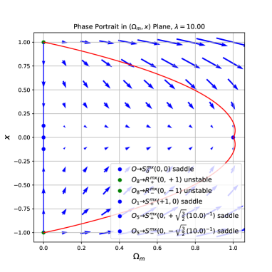
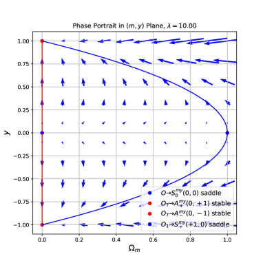
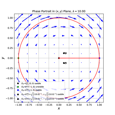
Figure 7: We illustrate the phase portrait of the 3D model, for $\lambda=+10$, which represents the $\lambda\in[+2,+\infty)$. Left Panel: We illustrate the phase portrait of the $(m,x)$. Center Panel: We illustrate the phase portrait of the $(m,y)$ Right Panel: We illustrate the phase portrait of the $(x,y)$. [See sections C.3.7, C.3.8, and C.3.9].

C.3.8 Phase portrait in $(m,y)$-plane, Case: high decreasing exponential scalar potential $\lambda\in[+2,+\infty)$

In Fig. 7, we find the results for the $(m,y)$-plane phase portrait for high decreasing exponential scalar potential, $\lambda=10$, which are the same as the results for $\lambda=\{-1,1\}$.

In particular, in Fig. 7, we plot the $(m,y)$-plane phase portrait, and we find the following points:

• The unstable point, $O\to R^{my}_{0}(0,0)$, is characterised by a vanishing matter energy density ratio, vanishing scalar kinetic energy density ratio, vanishing scalar potential energy density ratio, and dominant radiation energy density ratio.

• The stable point, $O_{7}\to A^{my}_{+}(0,1)$, is characterised by a vanishing matter energy density ratio, vanishing scalar kinetic energy density ratio, positively dominant scalar potential energy density ratio, and vanishing radiation energy density ratio.

• The stable point, $O_{7}\to A^{my}_{-}(0,-1)$, is characterised by a vanishing matter energy density ratio, vanishing scalar kinetic energy density ratio, negatively dominant scalar potential energy density ratio, and vanishing radiation energy density ratio.

• The saddle point, $O_{1}\to S^{my}_{+}(1,0)$, is characterised by a dominant matter energy density ratio, vanishing scalar kinetic energy density ratio, vanishing scalar potential energy density ratio, and vanishing radiation energy density ratio.

We observe that the dynamical field starts from the repeller $R^{my}_{0}(0,0)$ and they go towards the attractors $A^{my}_{+}(0,1)$ and $A^{my}_{-}(0,-1)$. The fields also go towards the saddle point $S^{my}_{+}(0,0)$, but they turn away before reaching it.

The physical picture is that we start with no matter energy density ratio $m=\Omega_{m}[N(t)]=0$ and no energy density ratio for potential term of the $V[t;N(t),\phi(N)]$-field, i.e. $V[t;N,\phi]\Leftrightarrow y^{2}=\Omega_{y^{2}}=0$, and then we move to a region where the energy density ratio for the potential term of the $V[t;N(t),\phi(N)]$-field becomes dominant, i.e. $V[t;N,\phi]\Leftrightarrow y^{2}=\Omega_{y^{2}}=\pm 1$, while we also move to a vanishing matter energy density ratio fo the kinetic term of the $m=\Omega_{m}[N(t)]=0$, while there is some increase in between.

This signifies the transition from a vanishing matter energy density ratio, vanishing scalar kinetic energy density ratio, vanishing scalar potential energy density ratio, and dominant radiation energy density ratio epoch, towards a vanishing matter energy density ratio, vanishing scalar kinetic energy density ratio, dominant scalar potential energy density ratio, and vanishing radiation energy density ratio epoch.

In other words, simply, this signifies the transition from a dominant radiation energy density ratio epoch, towards a dominant scalar potential energy density ratio epoch.

Note that the dominant scalar potential energy density ratio epoch corresponds to a $\Lambda$ energy density ratio domination epoch in the far future.

C.3.9 Phase portrait in $(x,y)$-plane, Case: high decreasing/increasing exponential scalar potential $\lambda\in[+2,+\infty)$

In Fig. 7, we plot the $(x,y)$-plane phase portrait for high decreasing exponential scalar potential $\lambda=10$, and we find similar but not the same results as in in the cases $\lambda=\{-1,0,1\}$. The difference, is that the attractors appear to negative values for energy density ratio for the kinetic term, $x$.

In particular, in Fig. 7, we plot the $(x,y)$-plane phase portrait, and we find the following points:

• The spiral CW point, $O_{8}\to R^{xy}_{0}(0,0)$, is characterised by a vanishing matter energy density ratio, vanishing scalar kinetic energy density ratio, vanishing scalar potential energy density ratio, and dominant radiation energy density ratio.

• The saddle point, $O_{9}\to S^{xy}_{+}(1,0)$, is characterised by a vanishing matter energy density ratio, positively dominant scalar kinetic energy density ratio, vanishing scalar potential energy density ratio, and vanishing radiation energy density ratio.

• The unstable point, $O_{8}\to R^{xy}_{-}(-1,0)$, is characterised by a vanishing matter energy density ratio, negatively dominant scalar kinetic energy density ratio, vanishing scalar potential energy density ratio, and vanishing radiation energy density ratio.

• The spiral CW point, $O_{5}\to R^{xy}_{+}(-\frac{1}{10}\sqrt{\frac{3}{2}},+\frac{1}{10}\sqrt{\frac{3}{2}})$, is characterised by a vanishing matter energy density ratio, negatively low dominant scalar kinetic energy density ratio, positively low scalar potential energy density ratio, and high dominant radiation energy density ratio.

• The spiral ACW point, $O_{5}\to R^{xy}_{-}(-\frac{1}{10}\sqrt{\frac{3}{2}},-\frac{1}{10}\sqrt{\frac{3}{2}})$, is characterised by a vanishing matter energy density ratio, negatively low dominant scalar kinetic energy density ratio, negatively low scalar potential energy density ratio, and high dominant radiation energy density ratio.

We observe that the dynamical field start from an unstable point, $R^{xy}_{-}(-1,0)$, and they go towards the saddle $S^{xy}_{+}(1,0)$. There are also the spiral CW $R^{xy}_{0}(0,0)$ and $R^{xy}_{+}(-\frac{1}{10}\sqrt{\frac{3}{2}},+\frac{1}{10}\sqrt{\frac{3}{2}})$ and spiral AntiClockwise ACW point $R^{xy}_{-}(-\frac{1}{10}\sqrt{\frac{3}{2}},-\frac{1}{10}\sqrt{\frac{3}{2}})$.

The physical picture is that we start with negatively maximum energy density ratio for the kinetic term of the $\phi[N(t)]$-field, i.e. $\dot{\phi}(t)\Leftrightarrow x^{2}=\Omega_{x^{2}}=0$ and no energy density ratio for potential term of the $V[t;N(t),\phi(N)]$-field, i.e. $V[t;N,\phi]\Leftrightarrow y^{2}=\Omega_{y^{2}}=0$, and then we move to a region where the energy density ratio for the potential term of the $V[t;N(t),\phi(N)]$-field becomes dominant, i.e. $V[t;N,\phi]\Leftrightarrow y^{2}=\Omega_{y^{2}}=\pm 1$, while we also move to a vanishing energy density ratio fo the kinetic term of the $\phi[N(t)]$-field, i.e. $\dot{\phi}(t)\Leftrightarrow x^{2}=\Omega_{x^{2}}=0$, and finally we land to a vanishing energy density ratio for the potential term and a maximum dominant energy density ratio for the kinetic term.

This signifies the transition from a vanishing matter energy density ratio, negatively dominant scalar kinetic energy density ratio, vanishing scalar potential energy density ratio, and vanishing radiation energy density ratio epoch towards a vanishing matter energy density ratio, positively dominant scalar kinetic energy density ratio, vanishing scalar potential energy density ratio, and vanishing radiation energy density ratio epoch.

In other words, simply, this signifies the transition from a negatively dominant scalar kinetic energy density ratio epoch towards a positively dominant scalar kinetic energy density ratio epoch.

C.3.10 Phase portrait in $(m,x)$-plane, Case: high decreasing/increasing exponential scalar potential $\lambda\in[-2,-\infty)$

In Fig. 8, we plot the $(m,x)$-plane phase portrait for high decreasing exponential scalar potential, $\lambda=-10$, and we find the similar results as in the cases $\lambda=\{-1,0,1,10\}$.

In Fig. 8, we plot the $(m,x)$-plane phase portrait, and we find the following points:

• The saddle point, $O\to S^{mx}_{0}(0,0)$, is characterised by a vanishing matter energy density ratio, vanishing scalar kinetic energy density ratio, vanishing scalar potential energy density ratio, and dominant radiation energy density ratio.

• The unstable point, $O_{8}\to R^{mx}_{+}(0,1)$, is characterised by a vanishing matter energy density ratio, positively dominant scalar kinetic energy density ratio, vanishing scalar potential energy density ratio, and vanishing radiation energy density ratio.

• The unstable point, $O_{8}\to R^{mx}_{-}(0,-1)$, is characterised by a vanishing matter energy density ratio, negatively dominant scalar kinetic energy density ratio, vanishing scalar potential energy density ratio, and vanishing radiation energy density ratio.

• The saddle point, $O_{1}\to A^{mx}_{0}(1,0)$, is characterised by a dominant matter energy density ratio, vanishing scalar kinetic energy density ratio, vanishing scalar potential energy density ratio, and vanishing radiation energy density ratio.

• The saddle point, $O_{4}\to S^{mx}_{+}(+\sqrt{\frac{3}{2}}(-10)^{-1},0)$, is characterised by a negatively low dominant matter energy density ratio, vanishing scalar kinetic energy density ratio, vanishing scalar potential energy density ratio, and dominant radiation energy density ratio.

• The saddle point, $O_{4}\to S^{mx}_{-}(-\sqrt{\frac{3}{2}}(-10)^{-1},0)$, is characterised by a positively low dominant matter energy density ratio, vanishing scalar kinetic energy density ratio, vanishing scalar potential energy density ratio, and dominant radiation energy density ratio.

We observe that the dynamical field starts from the repellers $R^{mx}_{+}(0,1)$ and $R^{mx}_{-}(0,-1)$ and they go towards the attractor $A^{mx}_{0}(1,0)$. The fields also go towards the saddle points $S^{mx}_{0}(0,0)$ $S^{mx}_{+}(+\sqrt{\frac{3}{2}}(-10)^{-1},0)$, $S^{mx}_{-}(-\sqrt{\frac{3}{2}}(-10)^{-1},0)$, but they turn away before reaching them.

The physical picture is that we start with some high energy density ratio for the kinetic term of the $\phi[N(t)]$-field, i.e. $\dot{\phi}(t)\Leftrightarrow x^{2}=\Omega_{x^{2}}=\pm 1$, while vanishing energy density ratio for matter of the universe, i.e. $m=\Omega_{m}[N(t)]=0$, and then we move to a region where energy density ratio for the kinetic term of the $\phi[N(t)]$-field vanishes, i.e. $\dot{\phi}(t)\Leftrightarrow x^{2}=\Omega_{x^{2}}=0$, while the energy density ratio for matter of the universe becomes dominant, i.e. $m=\Omega_{m}[N(t)]=1$.

This signifies the transition from a vanishing matter energy density ratio, dominant scalar kinetic energy density ratio, vanishing scalar potential energy density ratio, and vanishing radiation energy density ratio epoch, towards a dominant matter energy density ratio, vanishing scalar kinetic energy density ratio, vanishing scalar potential energy density ratio, and vanishing radiation energy density ratio epoch.

In other words, simply, this signifies the transition from a dominant scalar kinetic energy density ratio epoch, towards a dominant matter energy density ratio epoch.

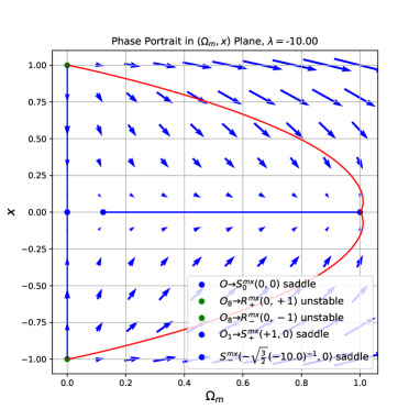
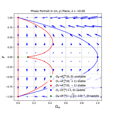
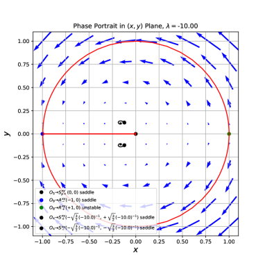
Figure 8: We illustrate the phase portrait of the 3D model, for $\lambda=-10$, which represents the $|\lambda|\in[-2,-\infty)$. Left Panel: We illustrate the phase portrait of the $(m,x)$. Center Panel: We illustrate the phase portrait of the $(m,y)$ Right Panel: We illustrate the phase portrait of the $(x,y)$. [See sections C.3.10, C.3.11, and C.3.12].

C.3.11 Phase portrait in $(m,y)$-plane, Case: high decreasing/increasing exponential scalar potential $\lambda\in[-2,-\infty)$

In Fig. 8, we find the results for the $(m,y)$-plane phase portrait for high increasing exponential scalar potential, $\lambda=-10$, which are similar but not the same as the results for $\lambda=\{-1,0,1,10\}$.

In particular, in Fig. 8, we plot the $(m,y)$-plane phase portrait, and we find the following points:

• The unstable point, $O_{8}\to R^{my}_{0}(0,0)$, is characterised by a vanishing matter energy density ratio, vanishing scalar kinetic energy density ratio, vanishing scalar potential energy density ratio, and dominant radiation energy density ratio.

• The stable point, $O_{7}\to A^{my}_{+}(0,1)$, is characterised by a vanishing matter energy density ratio, vanishing scalar kinetic energy density ratio, positively dominant scalar potential energy density ratio, and vanishing radiation energy density ratio.

• The stable point, $O_{7}\to A^{my}_{-}(0,-1)$, is characterised by a vanishing matter energy density ratio, vanishing scalar kinetic energy density ratio, negatively dominant scalar potential energy density ratio, and vanishing radiation energy density ratio.

• The saddle point, $O_{1}\to S^{my}_{0}(1,0)$, is characterised by a dominant matter energy density ratio, vanishing scalar kinetic energy density ratio, vanishing scalar potential energy density ratio, and vanishing radiation energy density ratio.

• The unstable point, $O_{4}\to R^{my}_{+}(+\sqrt{\frac{3}{2}}(-10)^{-1},0)$, is characterised by a negatively low dominant matter energy density ratio, vanishing scalar kinetic energy density ratio, vanishing scalar potential energy density ratio, and high dominant radiation energy density ratio.

• The unstable point, $O_{4}\to R^{my}_{-}(-\sqrt{\frac{3}{2}}(-10)^{-1},0)$, is characterised by a positively low dominant matter energy density ratio, vanishing scalar kinetic energy density ratio, vanishing scalar potential energy density ratio, and dominant radiation energy density ratio.

We observe that the dynamical field starts from the repellers $R^{my}_{0}(0,0)$ $R^{my}_{+}(+\sqrt{\frac{3}{2}}(-10)^{-1},0)$, $R^{m}_{-}(-\sqrt{\frac{3}{2}}(-10)^{-1},0)$ and they go towards the attractors $A^{my}_{+}(0,1)$ and $A^{my}_{-}(0,-1)$. The fields also go towards the saddle point $S^{my}_{0}(0,0)$, but they turn away before reaching it.

The physical picture is that we start with no matter energy density ratio $m=\Omega_{m}[N(t)]=0$, or low matter energy density ratio, $m=\Omega_{m}[N(t)]=\pm\sqrt{\frac{3}{2}}(-10)^{-1}$, and no energy density ratio for potential term of the $V[t;N(t),\phi(N)]$-field, i.e. $V[t;N,\phi]\Leftrightarrow y^{2}=\Omega_{y^{2}}=0$, and then we move to a region where the energy density ratio for the potential term of the $V[t;N(t),\phi(N)]$-field becomes dominant, i.e. $V[t;N,\phi]\Leftrightarrow y^{2}=\Omega_{y^{2}}=\pm 1$, while we also move to a vanishing matter energy density ratio, $m=\Omega_{m}[N(t)]=0$, while there is some increase in between.

This signifies the transition from a vanishing matter energy density ratio, vanishing scalar kinetic energy density ratio, vanishing scalar potential energy density ratio, and dominant radiation energy density ratio epoch and a epoch towards a vanishing matter energy density ratio, vanishing scalar kinetic energy density ratio, positively dominant scalar potential energy density ratio, and vanishing radiation energy density ratio epoch.

In other words, simply, this signifies the transition from a dominant radiation energy density ratio epoch and a low dominant matter energy density ratio and high dominant radiation energy density ratio epoch, towards a dominant scalar potential energy density ratio epoch.

Note that the dominant scalar potential energy density ratio epoch corresponds to a $\Lambda$ energy density ratio domination epoch in the far future.

C.3.12 Phase portrait in $(x,y)$-plane, Case: high decreasing/increasing exponential scalar potential $\lambda\in[-2,-\infty)$

In Fig. 8, we plot the $(x,y)$-plane phase portrait for high increasing exponential scalar potential, $\lambda=-10$, and we find similar but not the same results as in in the cases $\lambda=\{-1,0,1,10\}$. The difference, is that the attractors appear to negative values for energy density ratio for the kinetic term, $x$.

In particular, in Fig. 8, we plot the $(x,y)$-plane phase portrait, and we find the following points:

• The spiral CW point, $O_{5}\to S^{xy}_{p+}(0,0)$, is characterised by a vanishing matter energy density ratio, vanishing scalar kinetic energy density ratio, vanishing scalar potential energy density ratio, and dominant radiation energy density ratio.

• The unstable point, $O_{8}\to R^{xy}_{+}(1,0)$, is characterised by a vanishing matter energy density ratio, positively dominant scalar kinetic energy density ratio, vanishing scalar potential energy density ratio, and vanishing radiation energy density ratio.

• The stable point, $O_{9}\to A^{xy}_{-}(-1,0)$, is characterised by a vanishing matter energy density ratio, negatively dominant scalar kinetic energy density ratio, vanishing scalar potential energy density ratio, and vanishing radiation energy density ratio.

• The spiral CW point, $O_{4}\to R^{xy}_{+}(\frac{1}{-10}\sqrt{\frac{3}{2}},+\frac{1}{-10}\sqrt{\frac{3}{2}})$, is characterised by a vanishing matter energy density ratio, negatively low dominant scalar kinetic energy density ratio, negatively low scalar potential energy density ratio, and high dominant radiation energy density ratio.

• The spiral ACW point, $O_{4}\to R^{xy}_{-}(\frac{1}{-10}\sqrt{\frac{3}{2}},-\frac{1}{-10}\sqrt{\frac{3}{2}})$, is characterised by a vanishing matter energy density ratio, negatively low dominant scalar kinetic energy density ratio, positively low scalar potential energy density ratio, and high dominant radiation energy density ratio.

We observe that the dynamical field start from an unstable point, $R^{xy}_{+}(1,0)$, and they go towards the attractor $A^{xy}_{-}(-1,0)$. There are also the spiral CW $R^{xy}_{0}(0,0)$ and $R^{xy}_{+}(\frac{1}{-10}\sqrt{\frac{3}{2}},+\frac{1}{-10}\sqrt{\frac{3}{2}})$ and spiral AntiClockwise ACW point $R^{xy}_{-}(\frac{1}{-10}\sqrt{\frac{3}{2}},-\frac{1}{-10}\sqrt{\frac{3}{2}})$.

The physical picture is that we start with positively maximum energy density ratio for the kinetic term of the $\phi[N(t)]$-field, i.e. $\dot{\phi}(t)\Leftrightarrow x^{2}=\Omega_{x^{2}}=0$ and no energy density ratio for potential term of the $V[t;N(t),\phi(N)]$-field, i.e. $V[t;N,\phi]\Leftrightarrow y^{2}=\Omega_{y^{2}}=0$, and then we move to a region where the energy density ratio for the potential term of the $V[t;N(t),\phi(N)]$-field becomes dominant, i.e. $V[t;N,\phi]\Leftrightarrow y^{2}=\Omega_{y^{2}}=\pm 1$, while we also move to a vanishing energy density ratio fo the kinetic term of the $\phi[N(t)]$-field, i.e. $\dot{\phi}(t)\Leftrightarrow x^{2}=\Omega_{x^{2}}=0$, and finally we land to a vanishing energy density ratio for the potential term and a maximum negatively dominant energy density ratio for the kinetic term.

This signifies the transition from a vanishing matter energy density ratio, positively dominant scalar kinetic energy density ratio, vanishing scalar potential energy density ratio, and vanishing radiation energy density ratio epoch towards a vanishing matter energy density ratio, negatively dominant scalar kinetic energy density ratio, vanishing scalar potential energy density ratio, and vanishing radiation energy density ratio epoch.

In other words, simply, this signifies the transition from a positively dominant scalar kinetic energy density ratio epoch towards a negatively dominant scalar kinetic energy density ratio epoch.

References

- Schöneberg et al. [2022] Schöneberg, N., G. Franco Abellán, A. Pérez Sánchez, et al. The H0 Olympics: A fair ranking of proposed models. Phys. Rept., 984:1–55, 2022. arXiv:astro-ph.CO/2107.10291.
- Ntelis [2016a] Ntelis, P. The Homogeneity Scale of the universe. 2016a, arXiv:astro-ph.CO/1607.03418.
- Laurent et al. [2016] Laurent, P., J.-M. Le Goff, E. Burtin, et al. A 14 h-3 Gpc3 study of cosmic homogeneity using BOSS DR12 quasar sample. 2016. arXiv:1602.09010.
- Ntelis [2016b] Ntelis, P. The Homogeneity Scale Of The Universe. In 51st Rencontres de Moriond on Cosmology, pages 129--134. ARISF, 2016b.
- Ntelis et al. [2017] Ntelis, P., J.-C. Hamilton, J.-M. Le Goff, et al. Exploring cosmic homogeneity with the BOSS DR12 galaxy sample. Journal of Cosmology and Astroparticle Physics, 2017:019, 2017. arXiv:astro-ph.CO/1702.02159.
- Ntelis and Ealet [2018] Ntelis, P. and A. Ealet. Euclid: Homogeneity in the search of the Dark Sector. In 53rd Rencontres de Moriond on Cosmology, pages 367--370, 2018, arXiv:astro-ph.CO/1805.10441.
- Akrami et al. [2021] Akrami, Y. et al. Modified Gravity and Cosmology: An Update by the CANTATA Network. Springer, 2021, arXiv:gr-qc/2105.12582. ISBN 978-3-030-83714-3, 978-3-030-83717-4, 978-3-030-83715-0.
- Bahamonde et al. [2018] Bahamonde, S., C. G. Böhmer, S. Carloni, et al. Dynamical systems applied to cosmology: dark energy and modified gravity. Phys. Rept., 775-777:1--122, 2018. arXiv:gr-qc/1712.03107.
- Bahamonde et al. [2021] Bahamonde, S., V. Gakis, S. Kiorpelidi, et al. Cosmological perturbations in modified teleparallel gravity models: Boundary term extension. Eur. Phys. J. C, 81:53, 2021. arXiv:gr-qc/2009.02168.
- Bahamonde and Gigante Valcarcel [2021] Bahamonde, S. and J. Gigante Valcarcel. Observational constraints in metric-affine gravity. Eur. Phys. J. C, 81:495, 2021. arXiv:gr-qc/2103.12036.
- Aoki et al. [2023] Aoki, K., S. Bahamonde, J. Gigante Valcarcel, et al. Cosmological Perturbation Theory in Metric-Affine Gravity. 2023. arXiv:gr-qc/2310.16007.
- Bahamonde et al. [2023] Bahamonde, S., K. F. Dialektopoulos, C. Escamilla-Rivera, et al. Teleparallel gravity: from theory to cosmology. Rept. Prog. Phys., 86:026901, 2023. arXiv:gr-qc/2106.13793.
- Ntelis and Morris [2023] Ntelis, P. and A. Morris. Functors of Actions. Foundations of Physics, 53:29, 2023.
- Ntelis [2024] Ntelis, P. New avenues and observational constraints on functors of actions theories. PoS, EPS-HEP2023:104, 2024.
- Copeland et al. [1998] Copeland, E. J., A. R. Liddle, and D. Wands. Exponential potentials and cosmological scaling solutions. Phys. Rev. D, 57:4686--4690, 1998. arXiv:gr-qc/9711068.
- Ferreira and Joyce [1998] Ferreira, P. G. and M. Joyce. Cosmology with a primordial scaling field. Phys. Rev. D, 58:023503, 1998. arXiv:astro-ph/9711102.
- Copeland et al. [2006] Copeland, E. J., M. Sami, and S. Tsujikawa. Dynamics of dark energy. International Journal of Modern Physics D, 15:1753--1936, 2006.
- Chen et al. [2009] Chen, X.-m., Y.-g. Gong, and E. N. Saridakis. Phase-space analysis of interacting phantom cosmology. JCAP, 04:001, 2009. arXiv:gr-qc/0812.1117.
- Fadragas et al. [2014] Fadragas, C. R., G. Leon, and E. N. Saridakis. Dynamical analysis of anisotropic scalar-field cosmologies for a wide range of potentials. Class. Quant. Grav., 31:075018, 2014. arXiv:gr-qc/1308.1658.
- van de Bruck et al. [2016] van de Bruck, C., J. Mifsud, J. P. Mimoso, et al. Generalized dark energy interactions with multiple fluids. JCAP, 11:031, 2016. arXiv:gr-qc/1605.03834.
- Leon et al. [2022] Leon, G., A. Paliathanasis, E. N. Saridakis, et al. Unified dark sectors in scalar-torsion theories of gravity. Phys. Rev. D, 106:024055, 2022. arXiv:gr-qc/2203.14866.
- Ramadan et al. [2024] Ramadan, O. F., T. Karwal, and J. Sakstein. Attractive proposal for resolving the Hubble tension: Dynamical attractors that unify early and late dark energy. Phys. Rev. D, 109:063525, 2024. arXiv:astro-ph.CO/2309.08082.
- Billyard et al. [1999] Billyard, A. P., A. A. Coley, and J. E. Lidsey. Qualitative analysis of early universe cosmologies. J. Math. Phys., 40:5092, 1999. arXiv:gr-qc/9907043.
- Tutusaus et al. [2020] Tutusaus, I. et al. : The importance of galaxy clustering and weak lensing cross-correlations within the photometric survey. Astron. Astrophys., 643:A70, 2020. arXiv:astro-ph.CO/2005.00055.
- Ilić et al. [2022] Ilić, S. et al. Euclid preparation. XV. Forecasting cosmological constraints for the Euclid and CMB joint analysis. Astron. Astrophys., 657:A91, 2022. arXiv:astro-ph.CO/2106.08346.
- Mellier et al. [2024] Mellier, Y. et al. Euclid. I. Overview of the Euclid mission. 2024. arXiv:astro-ph.CO/2405.13491.
- Alam et al. [2021] Alam, S. et al. Towards testing the theory of gravity with DESI: summary statistics, model predictions and future simulation requirements. JCAP, 11:050, 2021. arXiv:astro-ph.CO/2011.05771.
- Basilakos et al. [2019] Basilakos, S., G. Leon, G. Papagiannopoulos, et al. Dynamical system analysis at background and perturbation levels: Quintessence in severe disadvantage comparing to CDM. Phys. Rev. D, 100:043524, 2019. arXiv:gr-qc/1904.01563.