DESI Strong Lens Foundry I:
HST Observations and Modeling with GIGA-Lens

Abstract

We present the Dark Energy Spectroscopic Instrument (DESI) Strong Lens Foundry. We discovered $\sim 3500$ new strong gravitational lens candidates in the DESI Legacy Imaging Surveys using residual neural networks (ResNet). We observed a subset (51) of our candidates using the Hubble Space Telescope (HST). All of them were confirmed to be strong lenses. We also briefly describe spectroscopic follow-up observations by DESI and Keck NIRES programs. From this very rich dataset, a number of studies will be carried out, including evaluating the quality of the ResNet search candidates and lens modeling. In this paper, we present our initial effort in these directions. In particular, as a demonstration, we present the lens model for DESI-165.4754-06.0423, with imaging data from HST, and lens and source redshifts from DESI and Keck NIRES, respectively. In this effort, we have applied a fully forward-modeling Bayesian approach (GIGA-Lens), using multiple GPUs, for the first time in both regards, to a strong lens with HST data, or any high resolution imaging.

1 Introduction

Strong gravitational lensing systems are a powerful tool for astrophysics and cosmology. They have been used to study how dark matter is distributed in galaxies and galaxy clusters (e.g., Kochanek, 1991; Blandford & Narayan, 1992; Broadhurst et al., 2000; Koopmans & Treu, 2002; Bolton et al., 2006; Clowe et al., 2006; Koopmans et al., 2006; Bradač et al., 2008; Vegetti & Koopmans, 2009; Huang et al., 2009; Jullo et al., 2010; Tessore et al., 2016; Monna et al., 2017; Jauzac et al., 2018; Shajib et al., 2019; Meneghetti et al., 2020). Furthermore, carefully modeling the mass profiles of galaxy-scale strong lenses for a large number of lensing systems over a wide range of redshifts makes it possible to study the structural evolution of massive elliptical galaxies (e.g., Bolton et al., 2012; Sonnenfeld et al., 2013; Li et al., 2018; Filipp et al., 2023). They are also uniquely suited to probe dark matter substructure beyond the local universe and line-of-sight low-mass halos (e.g., Vegetti et al., 2014; Hezaveh et al., 2016; Vegetti et al., 2018; Ritondale et al., 2019; Diaz Rivero & Dvorkin, 2020; Çaǧan Şengül et al., 2022; Nierenberg et al., 2023), to test the predictions of the cold dark matter (CDM) model.

Recent measurements of the Hubble constant $H_{0}$ span a range of $\sim$10% (e.g., Abbott et al., 2017, 2018a; Riess et al., 2019; Wong et al., 2019; Freedman et al., 2019, 2020; Planck Collaboration et al., 2020; Khetan et al., 2021; Philcox et al., 2021; Choi et al., 2020; Dhawan et al., 2023), and significant tension between predictions for $H_{0}$ based on early-universe observables and direct late-universe measurements remain (e.g., Verde et al., 2019). Multiply-lensed supernovae (SNe) are ideal for measuring time-delays and $H_{0}$ because of their well-characterized light curves, and in the case of Type Ia, with the added benefit of standardizable luminosity (Refsdal, 1964; Treu, 2010; Oguri & Marshall, 2010; Suyu et al., 2024). In recent years, strongly lensed supernovae, both core-collapse (Kelly et al., 2015; Rodney et al., 2016) and Type Ia (Quimby et al., 2014; Goobar et al., 2017; Rodney et al., 2021; Chen et al., 2022; Goobar et al., 2023; Pierel et al., 2023; Frye et al., 2024), have been discovered. Retrospective searches have found lensed SNe as well, including Type Ia’s (Sheu et al., 2023; Magee et al., 2023). Time-delay from multiply imaged supernovae can therefore be an important independent way to constrain $H_{0}$ and address this tension in its measurements (e.g., Goldstein & Nugent, 2017; Goldstein et al., 2018, 2019; Wojtak et al., 2019; Pierel & Rodney, 2019; Suyu et al., 2020). In fact, Kelly et al. (2023) and Pascale et al. (2024) reported the first two measurements of $H_{0}$ using lensed SNe. Moreover, time-delay $H_{0}$ measurements are a powerful complement to other independent measurements of the dark energy equation of state (e.g., Linder, 2011; Treu & Marshall, 2016; Pierel et al., 2021). Both for cluster/group and galaxy-scale lenses, to systematically discover lensed SNe, we can monitor a sample of strong lenses with the highest estimated supernova rates for the lensed sources (e.g., Shu et al., 2018, 2021; Suyu et al., 2024).

Static strong lenses can be used to constrain cosmological parameters as well. Li et al. (2024) showed a large sample, $\mathcal{O}(10^{4})$, in combination with velocity dispersion measurements, can provide competitive constraints, including for the possible evolution of dark energy (e.g., Chevallier & Polarski, 2001; Linder, 2003). Compound lenses, lensing systems with two or more sources at different redshifts, are extremely valuable. Even a relatively small sample constitutes a powerful cosmological probe (e.g., Collett et al., 2012; Collett & Auger, 2014; Linder, 2016; Sharma & Linder, 2022; Sharma et al., 2023). Compared with a typical strong lens, with a single source, these are much rarer, and yet there have been some very promising recent discoveries (Sheu et al., 2024; Dux et al., 2024; Bolamperti et al., 2024).

Finally, for nearby strong lensing galaxies, extra-galactic tests of General Relativity can be performed by combining lens modeling with spatially resolved stellar kinematic observations (Collett et al., 2018).

For many of these analyses, the available sample size of confirmed strong lenses is a major limiting factor. In the last few years, several groups have used convolutional neural networks to search for strong lensing systems in photometric surveys, including, in increasing sky coverage, CFHTLS (Jacobs et al., 2017), KiDS (Petrillo et al., 2017, 2019; Li et al., 2020), DES (Jacobs et al., 2019a, b), and Pan-STARRS (Cañameras, R. et al., 2020).

The DESI Legacy Surveys (Dey et al., 2019), for which at least $z$ band is observed with 4-m telescopes, covers $\sim$19,000 deg², almost four times the size of the Dark Energy Survey (The Dark Energy Survey Collaboration, 2005) footprint. We identified over $\sim 3500$ new strong lenses in the Legacy Surveys (Huang et al., 2020, 2021; Storfer et al., 2024, respectively; henceforth, H20, H21, S24) by using residual neural networks. We have also found 436 lensed quasars (Dawes et al., 2023) using autocorrelation for a lensed quasar candidate sample. The entire catalog of these lens candidates can be found on our project website.

With so many lens discoveries, a fast and robust modeling pipeline is needed. We therefore developed GIGA-Lens (Gu et al., 2022): a GPU-accelerated, fully forward-modeling Bayesian pipeline that can speed up the lens modeling time by two orders of magnitude or more. Recently, we applied GIGA-Lens to an observed lensing system, DESI-253.2534+26.8843 (Cikota et al., 2023), making it the first real lens to be modeled by GPUs.

Here, we present the DESI Strong Lens Foundry project. With thousands of lens candidates, we can choose the best ones for the purposes of 1) detecting low-mass DM halos and 2) measuring $H_{0}$ — using the best lensed quasar systems and through a future targeted search for live lensed supernovae among lensing systems that are the most likely to host them. For high resolution imaging, our Hubble Space Telescope SNAP program (ID: 15867, PI: Huang) has observed a subset of the best candidates. In this paper — Paper I of this series — we describe our HST program. We will also present the first model using GPUs for a strong lensing system with HST data. Spectroscopic observations are also being carried out. The first spectroscopic results from the Dark Energy Spectroscopic Experiment (DESI; DESI Collaboration et al., 2016a, b) strong lens program will be presented in Paper II of this series (Huang, Inchausti et al., in prep). For $\sim 30\%$ of the systems (preliminary estimate), the source redshifts are too high, such that the typical emission features (e.g., [O II]) are beyond the DESI wavelength range. For these, our near-IR spectroscopic results from the Keck 2 Telescope will be reported in Paper III in this series (Agarwal et al., in prep).

This paper is organized as follows. We present our Hubble Space Telescope SNAP program in § 2, followed by a brief description of the DESI and Keck spectroscopic observations in § 3. In § 4, we present the model for one of our HST systems using GIGA-Lens. Our findings are discussed in § 5 and the conclusion is provided in § 6.

2 Hubble Space Telescope SNAP Program

In this section, we briefly describe our lens discoveries in the DESI Legacy Imaging Surveys in § 2.1 and present the follow-up HST SNAP program observations in § 2.2. All the HST data used in this paper can be found in MAST: http://dx.doi.org/10.17909/hx0v-9260 (catalog 10.17909/hx0v-9260).

2.1 Lens Discoveries in the DESI Legacy Imaging Surveys

The DESI Legacy Imaging Surveys (hereafter Legacy Surveys) are composed of three surveys: the Dark Energy Camera Legacy Survey (DECaLS), the Beijing-Arizona Sky Survey (BASS), and the Mayall $z$-band Legacy Survey (MzLS). DECaLS is observed by the Dark Energy Camera (DECam; Flaugher et al., 2015) on the 4-m Blanco telescope, which covers $\sim 9000$ deg² of the sky in the range of $-18^{\circ}\lesssim\delta\lesssim+32^{\circ}$. The MzLS has imaged the $\delta\gtrsim+32^{\circ}$ sub-region ($\sim 5000$ deg²) in $z$-band by the Mosaic3 camera (Dey et al., 2016) that complemented the BASS $g$- and $r$-band observations in the same sub-region on 90Prime camera (Williams et al., 2004) on the Bok 2.3-m telescope. Data Releases 9 & 10 (DR9, 10; Schlegel et al., in prep) contain additional DECam data reprocessed from the Dark Energy Survey (DES; Abbott et al., 2018b) for $\delta\lesssim-18^{\circ}$. This provides an extra $\sim 5000\leavevmode\nobreak\$deg², resulting in a total footprint of $\sim 19,000$ deg². The Legacy Surveys are imaged to a total depth of at least 22.5 AB mag in $z$-band (for galaxies with an exponential disk profile and a half-light radius r${}_{half}=0.45^{\prime\prime}$). The average FWHMs for the delivered images are: $1.29^{\prime\prime}$ ($g$), 1.18^′′ ($r$), and 1.11^′′ ($z$) for DECaLS; $1.61^{\prime\prime}$ ($g$) and $1.47^{\prime\prime}$ ($r$) for BASS; and $1.01^{\prime\prime}$ ($z$) for MzLS. A more detailed description of the Legacy Surveys can be found on the Legacy Surveys website. On this dataset, we have performed three lens searches in the Legacy Surveys in Data Releases 7, 8, and 9 (H20, H21, S24, respectively). We used a residual neural network architecture first developed by Lanusse et al. (2018), and improved upon by H21 (the “shielded” model). For all three searches, we used observed images of both lenses and non-lenses (instead of simulations or a combination of observations and simulations) for training.

2.2 Hubble Space Telescope Observations

We submitted a subset of our most promising lens candidates (112 targets) for the Hubble SNAP program GO-15867 (PI: Huang), Confirming Strong Galaxy Gravitational Lenses in the DESI Legacy Imaging Surveys. HST not only provides higher angular resolution, but reaches fainter surface brightness due to the fainter background in space. This can reveal the presence of lensed galaxies with lower surface brightness, including those at higher redshifts that have been dimmed by $(1+z)^{4}$. In addition, a NIR filter was chosen to make possible the detection of higher redshift sources that are beyond the optical ($grz$) reach of the DESI Legacy Surveys. These two factors expand the depth and redshift range of detectable arcs. Indeed, for a large number of systems in this program, the HST NIR observations revealed additional lensed sources, often with a larger Einstein radius than the one seen in the respective discovery $grz$ images. The targets were chosen for two main science goals. One, identifying the best systems for a future targeted search for lensed supernovae to measure the Hubble constant (e.g., Shu et al., 2018, 2021). Lensed supernovae have been discovered in galaxy-scale (e.g., Goobar et al., 2023; Pierel et al., 2023), and cluster-scale lenses (e.g., Kelly et al., 2023; Frye et al., 2024). Two, low-mass halo ($<10^{9}M_{\odot}$) detection. This is a powerful test of the cold dark matter (CDM) model, which predicts an abundance of low-mass halos, as subhalos or line-of-sight interlopers. These do not host a galaxy and hence are invisible. Beyond our local universe, they are only detectable by their gravitational effect, especially in strong lensing systems (e.g., Vegetti et al., 2010; Çaǧan Şengül et al., 2022). For this purpose, systems with a single galaxy as the main lens is usually preferred, as these are considered to be easier to model and hence can yield low-mass halo detection with greater confidence. However, cluster-scale lenses have been used for this purpose too (e.g., Dai et al., 2020). To the degree possible, using the ground-based Legacy Surveys images, we chose half of our HST targets to be galaxy-scale lenses and the other half, group/small cluster lenses. Among strong lenses, being in-between galaxy-scale and cluster-scale, the latter category is somewhat understudied. For example, in the SL2S program, 26 group-scale lenses were followed up with HST observations (More et al., 2012, Table 3). Our program in the end observed a comparable number of group/small cluster lenses. This is likely due to the fact that these systems are outside of the previous selection windows: galaxy-scale lenses were discoverable in highly multiplexed fiber spectroscopy and cluster-scale lenses are more readily identified by eye in deep images. In contrast, neural net based search methods applied to ground-based observations have discovered an abundance of strong lenses at the group to small cluster scales. We would like to explore its potential for these two science goals.

All targets have $3\times$399.23 sec exposure, for a total of 1197.7 sec, on WFC3 using the F140W filter in the NIR channel. The targets were approximately centered in the WFC3 aperture, with no CR split, because we wanted to keep read noise down. Of the 112 systems submitted to HST, a total of 53 were targeted. Two of them were not successfully observed due to the loss of the guide star. Of the 51 systems successfully observed, HST confirmed all of them to be strong lenses, by revealing one or more arcs in each. The native pixel size is $0.13^{\prime\prime}$, and each image is drizzled to $0.065^{\prime\prime}$. In this Hubble sample, DESI-025.4848+30.7585 has the faintest arcs. It has a lens redshift of $z_{d}=0.524$ from the extended Baryon Oscillation Spectroscopic Survey (eBOSS), which is further confirmed by DESI spectroscopy. In the Legacy Surveys discovery image (see Figure 2.2), there appear to be a lensed arc (arc 1) to the SE of the elliptical galaxy at the center and a hint of a small arc (arc 2) to the NW of and just above the same elliptical galaxy. Both are confirmed in the HST image. But HST also reveals that just below arc 2, even closer to the lens, there appears to be a third arc (arc 3). DESI provides the redshift for arc 1 ($z_{s,1}=1.2223$, based on clear detection of the [O II] doublet emission from DESI Year 1 data). Talbot et al. (2021) analyzed the lens spectrum closely and found evidence for emission lines of a lensed source in the same eBOSS fiber, and determined its redshift at $z_{s,2}=1.216$. The eBOSS fiber is $2^{\prime\prime}$ in diameter (Dawson et al., 2016), and thus is capable of detecting emission features for an arc $\lesssim 1^{\prime\prime}$ away from the lens. Therefore this redshift corresponds to either arc 3 ($0.87^{\prime\prime}$ from the lens) or arc 2 (at a distance of $1.20^{\prime\prime}$). Arc 1 at 2.10^′′ is not likely. In addition to this system, we will also provide spectroscopic redshifts from DESI and Keck for DESI-165.4754-06.0423 (see Figure 2.2), for which we will show a lens model in § 4. DESI redshifts for other systems will be presented in Paper II and future publications.

Figure 2.2 shows the first eight systems in this sample. These eight are representative of the type of lensing configuration for this HST sample. We show the rest of the 51 systems in Figures 2.2 - 2.2. There are a number of striking systems. In Figure 2.2, for DESI-004.2564-10.1530 and DESI-023.6765+04.5639, both group lenses, compared with the discovery images from the Legacy Surveys in the optical bands of $grz$, the HST NIR images reveal additional fainter arcs in each. This is true for a number of group-scale lensing systems in this sample. DESI-072.0873-19.4172 (Figure 2.2) is an Einstein cross with a remarkable average lens-image separation of 3.95^′′. The photometric redshift for the lens is $z_{d,phot}=0.967\pm 0.167$. There appear to be at least three other elliptical galaxies with similar colors (and therefore similar redshifts) within or near the Einstein cross, though they are considerably smaller. Inspection of the environment around this system shows that the lensing galaxy is at the center of a high redshift cluster. The presence of the Einstein cross, rarely seen for a group/cluster scale lens (e.g., Sheu et al., 2024, which shows an Einstein cross for a cluster lens with $z_{d}=0.49$), indicates that mass distribution is relaxed and highly symmetric within the Einstein radius, perhaps all the more unusual at such a high redshift. The modeling of this system is currently underway. Other notable systems include: a galaxy-scale lensing system that possibly has two multiply-imaged sources (DESI-133.3800+23.3652 in Figure 2.2, shown with arrows) and two group-scale systems with multiple images of a background galaxy with complex structure (DESI-189.5370+15.0309 in Figure 2.2 with a doubly imaged background spiral galaxy, or two half “cinnamon buns”, and DESI-327.8408+13.7884 in Figure 2.2, showing great details of a triply lensed spiral galaxy, which suggests a possible naked cusp configuration (e.g., Lewis et al., 2002). Finally, the HST image of DESI-254.4235+34.8162 (Figure 2.2) possibly reveals a radial counter arc very close to the lensing galaxy.

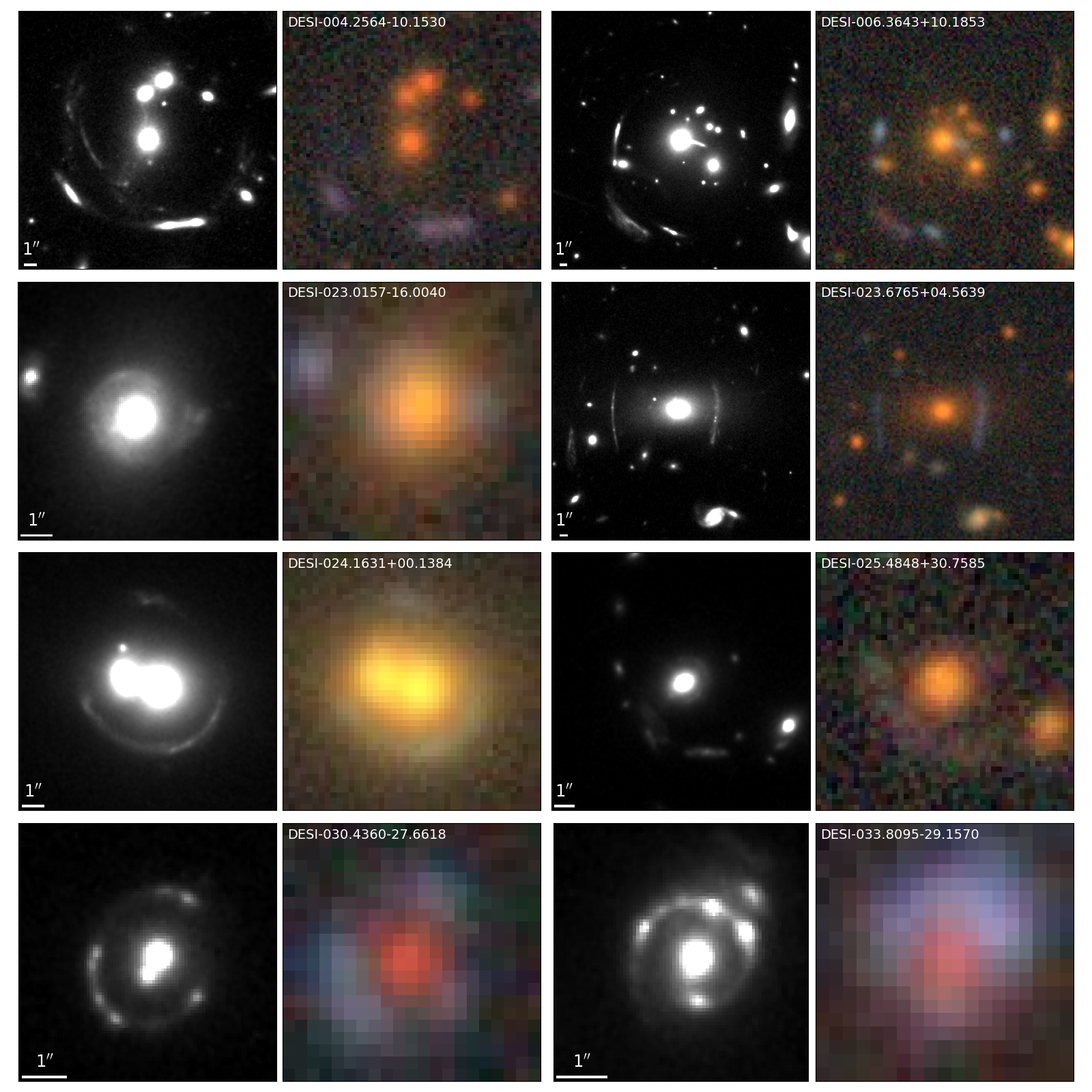
Figure 1: The first eight of the 51 systems observed by the HST SNAP program GO-15867. All were confirmed to be strong lenses by HST with arc(s) in each clearly revealed. For this and the next five figures (up to and including Figure 2.2): The naming convention is RA and Dec in decimal format. North is up, and East to the left. The systems are arranged in ascending RA. For each, we show the HST WFC3 NIR F140W image (left) and the Legacy Surveys optical image in $grz$ bands (right; these were the discovery images). The eight systems in this panel are representative of the 51 systems in this HST program: There are three group/small cluster scale lenses, DESI-004.2564-10.1530, DESI-006.3643+10.1853, and DESI-023.6765+04.5639. For each of them, there are at least two sets of arcs. Compared with the Legacy Surveys optical image, the NIR HST image revealed new arcs for the first and third system. DESI-023.0157-16.0040, DESI-025.4848+30.7585, and DESI-033.8095-29.1570 are galaxy-scale lens (for more on the lensing nature of DESI-025.4848+30.7585, see text). Finally, DESI-024.16341+00.1384 and DESI-030.4360-27.6618 each have two very close-by elliptical galaxies as the lens.

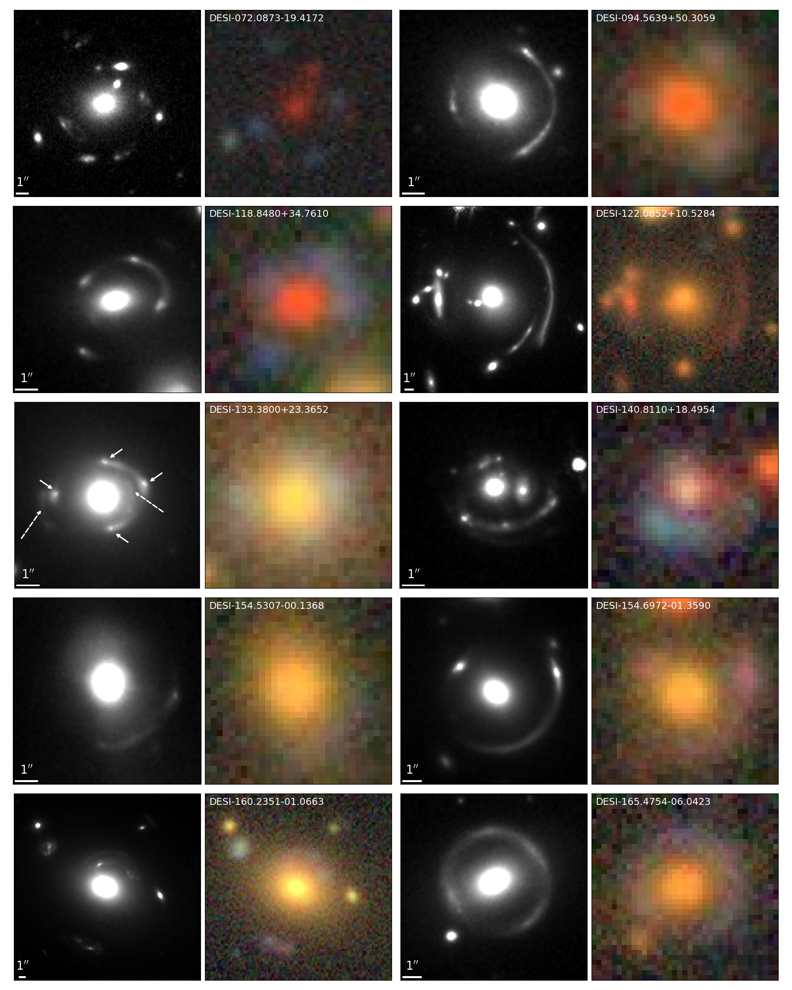
Figure 2: The next 10 (

#

9 –

#

18) of the 51 systems in HST GO-15867. For details, see the caption of Figure 2.2. The lens model for DESI-165.4754-06.0423 is presented in § 4. DESI-133.3800+23.3652 is a galaxy-scale lens, likely with two sources: one quadruply lensed (solid arrows) and one doubly lensed (dashed arrows).

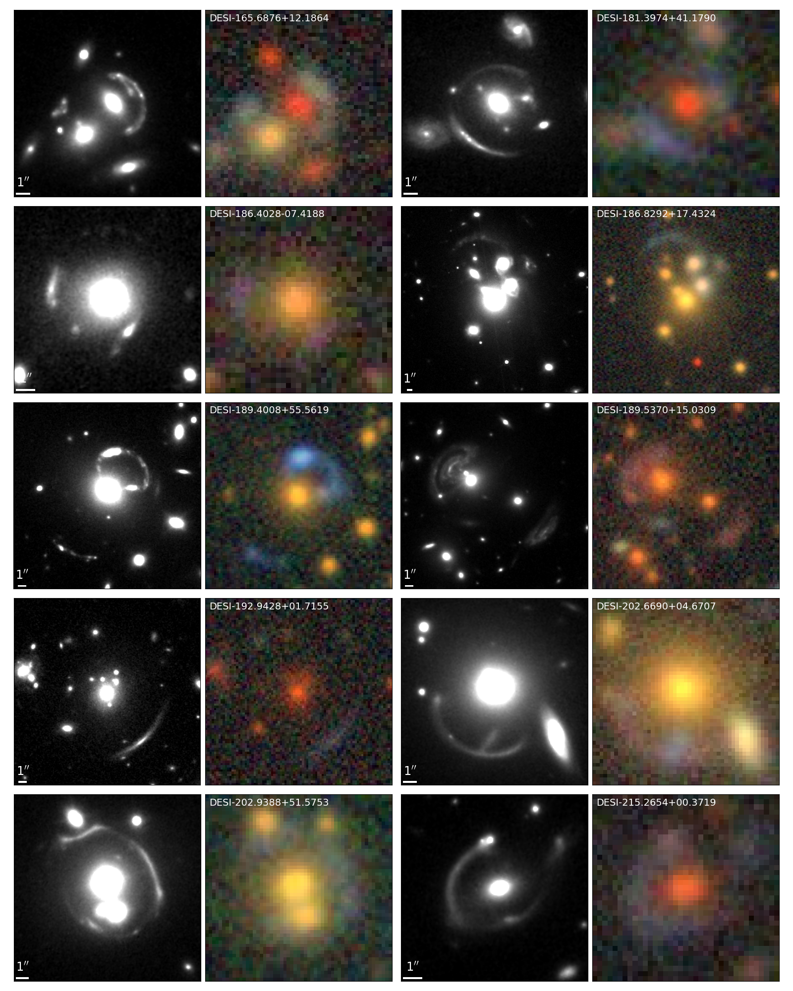
Figure 3: Systems

#

19 -

#

28 of the 51 in HST GO-15867. For details, see the caption of Figure 2.2. Note that DESI 189.5370+15.0309 shows a doubly imaged background spiral galaxy with complex structure, resembling two half “cinnamon buns”, with different sizes.

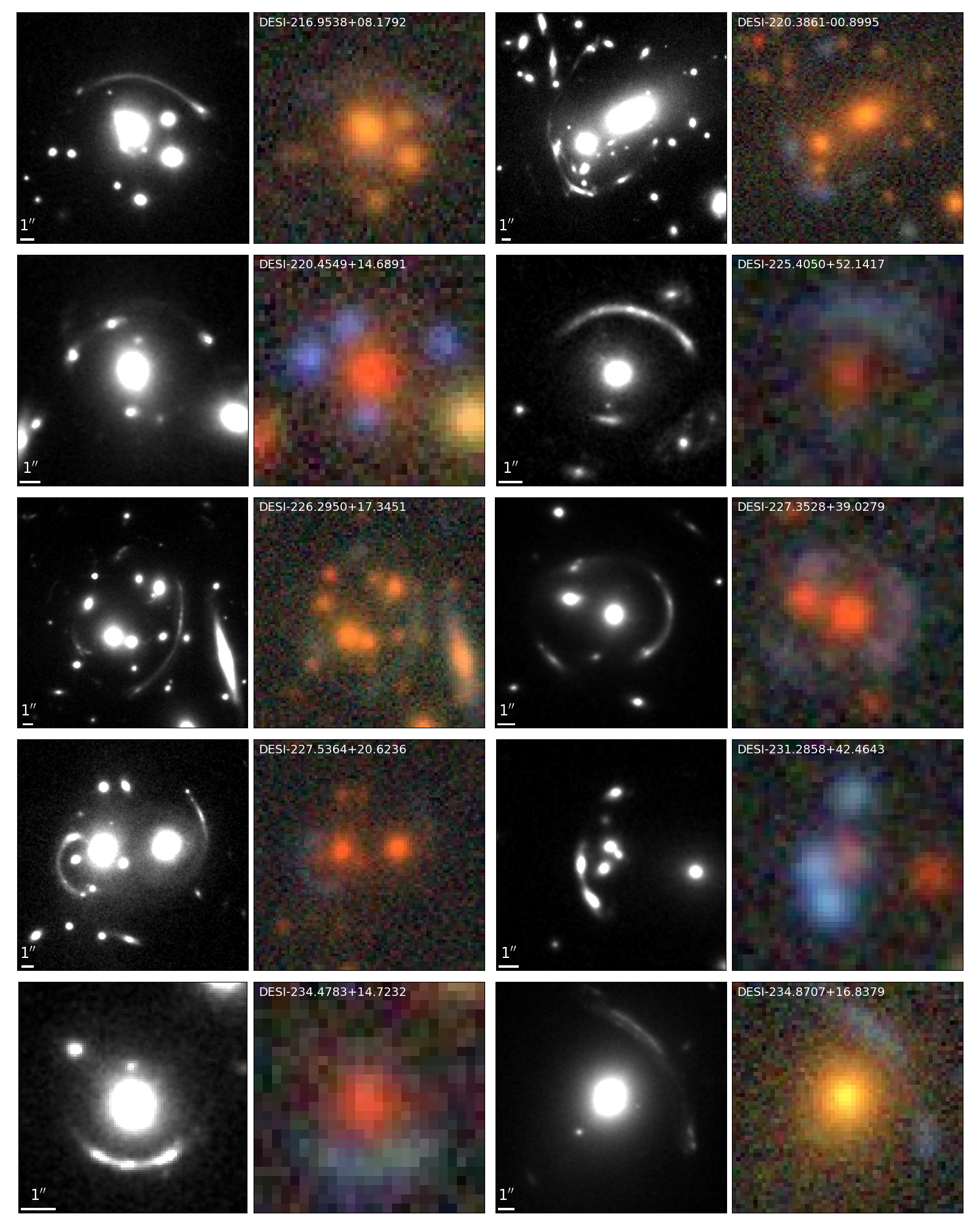
Figure 4: Systems

#

29 –

#

38 of the 51 in HST GO-15867. For details, see the caption of Figure 2.2.

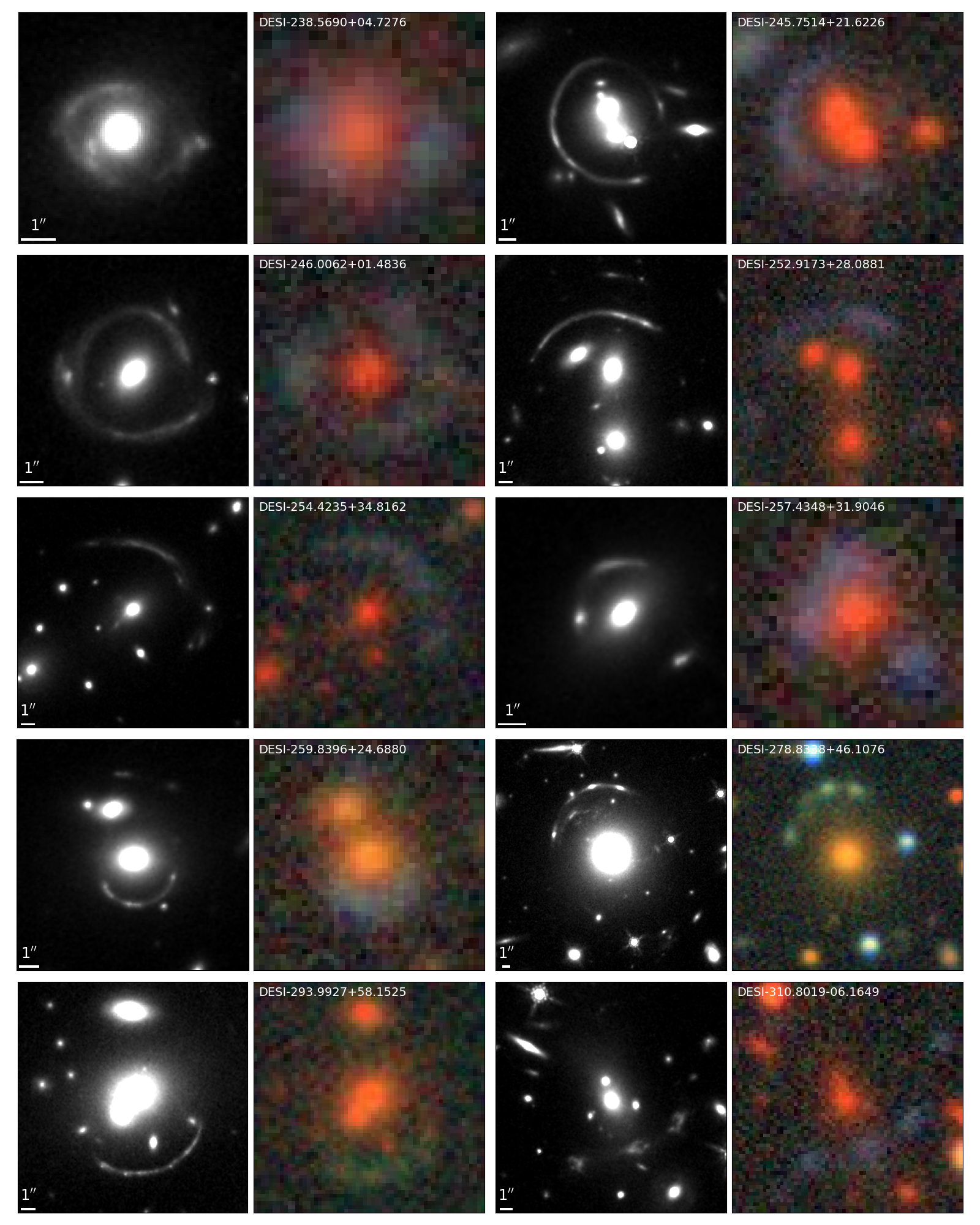
Figure 5: Systems

#

39 –

#

48 of the 51 in HST GO-15867. For details, see the caption of Figure 2.2. Note DESI-238.5690+04.7276, a galaxy-scale lens, likely with two lensed sources, which are quadruply (fainter) and doubly (brighter) lensed, respectively.

Figure 6: Systems

#

49 -

#

51 of the 51 in HST GO-15867. For details, see the caption of Figure 2.2. Note that DESI-327.8408+13.7884 shows a triply lensed galaxy around a group lens (see text), revealing great details of the magnified background spiral galaxy.

We present HST photometry for the brightest lensed source images for the source identified in the discovery image for all 51 systems in Table 1, where we define the contour to be at 75% of the peak pixel value. To account for the luminosity contribution from the lens we employ GALFIT (Peng et al., 2010), a parametric 2D fitting algorithm. We model the light components of the lensing galaxy using the Sérsic luminosity profile (Sérsic, 1963). Each Sérsic component in the fitting algorithm is described by the 7 parameters: $(x,y)$ position, integrated magnitude $m$, effective radius $r_{e}$, concentration index $n$, axis ratio $q$, and position angle $\theta$.

Prior to the fitting procedure, a PSF was generated for each image by stacking star cutouts from the field and iteratively refining a proposed PSF model based on the stack. This process was carried out using PSFr in the Lenstronomy package (Birrer et al., 2021). Following successful extraction of PSFs, each galaxy was initially fit using a single Sérsic component, with additional components added when necessary to adequately subtract the lens light from the image. Goodness of fit was determined using the $\chi^{2}$ metric as well as visual inspection of the image residuals. In cases where model parameters deviated from physically acceptable values, such as extreme $r_{e}$, constraints were imposed. For systems where the lensing field was densely populated, the light profiles of all galaxies in the image region were also modeled and subtracted to reduce contamination of source light. Moreover, in certain outlier cases where two source images appeared in close proximity to each other, the source light for such systems was also modeled in order to properly isolate each source image. Source light distribution was modeled using Sérsic profiles along with an additional bending mode where necessary.

Table 1: Isophotal magnitudes for the brightest source image

Target Name	RA (deg)	Dec (deg)	F140W Isophotal Magnitude (AB mag)	Contour Area (arcsec2)
DESI-004.2564-10.1530	4.2560	$-$10.1549	23.51 $\pm$ 0.02	0.0380
DESI-006.3643+10.1853	6.3646	10.1820	23.79 $\pm$ 0.02	0.0338
DESI-023.0157-16.0040	23.0152	$-$16.0041	25.04 $\pm$ 0.04	0.0634
DESI-023.6765+04.5639	23.6753	4.5635	25.68 $\pm$ 0.05	0.0338
DESI-024.1631+00.1384	24.1628	0.1376	24.89 $\pm$ 0.04	0.0380
DESI-025.4848+30.7585	25.4846	30.7587	26.43 $\pm$ 0.07	0.0423
DESI-030.4360-27.6618	30.4365	$-$27.6617	25.43 $\pm$ 0.05	0.0211
DESI-033.8095-29.1570	33.8094	$-$29.1571	24.16 $\pm$ 0.03	0.0169
DESI-072.0873-19.4172	72.0883	$-$19.4177	26.20 $\pm$ 0.06	0.0296
DESI-094.5639+50.3059	94.5634	50.3065	24.88 $\pm$ 0.04	0.0211
DESI-118.8480+34.7610	118.8477	34.7615	24.64 $\pm$ 0.03	0.0338
DESI-122.0852+10.5284	122.0836	10.5279	22.43 $\pm$ 0.01	0.5197
DESI-133.3800+23.3652	133.3795	23.3653	23.98 $\pm$ 0.02	0.0296
DESI-140.8110+18.4954	140.8114	18.4951	24.35 $\pm$ 0.03	0.0423
DESI-154.5307-00.1368	154.5299	$-$0.1369	25.42 $\pm$ 0.05	0.0296
DESI-154.6972-01.3590	154.6977	$-$1.3587	23.24 $\pm$ 0.02	0.0296
DESI-160.2351-01.0663	160.2353	$-$1.0654	23.55 $\pm$ 0.02	0.0423
DESI-165.4754-06.0423	165.4760	$-$6.0425	23.87 $\pm$ 0.02	0.1394
DESI-165.6876+12.1864	165.6870	12.1865	25.02 $\pm$ 0.04	0.0211
DESI-181.3974+41.1790	181.3981	41.1783	24.47 $\pm$ 0.03	0.0465
DESI-186.4028-07.4188	186.4026	$-$7.4193	24.92 $\pm$ 0.04	0.0296
DESI-186.8292+17.4324	186.8287	17.4343	24.13 $\pm$ 0.02	0.2113
DESI-189.4008+55.5619	189.4036	55.5601	24.26 $\pm$ 0.03	0.0380
DESI-189.5370+15.0309	189.5388	15.0313	23.81 $\pm$ 0.02	0.0676
DESI-192.9428+01.7155	192.9417	1.7138	23.59 $\pm$ 0.02	0.1648
DESI-202.6690+04.6707	202.6700	4.6698	23.74 $\pm$ 0.02	0.1310
DESI-202.9388+51.5753	202.9371	51.5752	23.32 $\pm$ 0.02	0.1817
DESI-215.2654+00.3719	215.2652	0.3715	24.39 $\pm$ 0.03	0.0845
DESI-216.9538+08.1792	216.9525	8.1795	24.21 $\pm$ 0.03	0.0507
DESI-220.3861-00.8995	220.3884	$-$0.9006	23.94 $\pm$ 0.02	0.0507
DESI-220.4549+14.6891	220.4557	14.6893	23.74 $\pm$ 0.02	0.0338
DESI-225.4050+52.1417	225.4047	52.1424	24.97 $\pm$ 0.04	0.0380
DESI-226.2950+17.3451	226.2932	17.3455	24.68 $\pm$ 0.03	0.0549
DESI-227.3528+39.0279	227.3521	39.0273	23.91 $\pm$ 0.02	0.0507
DESI-227.5364+20.6236	227.5339	20.6244	23.74 $\pm$ 0.02	0.1099
DESI-231.2858+42.4643	231.2877	42.4639	23.08 $\pm$ 0.02	0.0465
DESI-234.4783+14.7232	234.4780	14.7227	25.12 $\pm$ 0.04	0.0254
DESI-234.8707+16.8379	234.8703	16.8391	24.47 $\pm$ 0.03	0.0803
DESI-238.5690+04.7276	238.5695	4.7277	24.24 $\pm$ 0.03	0.1352
DESI-245.7514+21.6226	245.7524	21.6224	23.71 $\pm$ 0.02	0.0887
DESI-246.0062+01.4836	246.0060	1.4843	24.97 $\pm$ 0.04	0.0803
DESI-252.9173+28.0881	252.9166	28.0890	24.45 $\pm$ 0.03	0.0634
DESI-254.4235+34.8162	254.4234	34.8174	24.00 $\pm$ 0.02	0.1732
DESI-257.4348+31.9046	257.4352	31.9046	24.13 $\pm$ 0.02	0.0380
DESI-259.8396+24.6880	259.8397	24.6873	24.94 $\pm$ 0.04	0.0338
DESI-278.8338+46.1076	278.8348	46.1099	23.52 $\pm$ 0.02	0.0423
DESI-293.9927+58.1525	293.9930	58.1510	26.15 $\pm$ 0.06	0.0211
DESI-310.8019-06.1649	310.8015	$-$6.1660	23.86 $\pm$ 0.02	0.1648
DESI-327.8408+13.7884	327.8425	13.7896	23.67 $\pm$ 0.02	0.0465
DESI-329.6820+02.9584	329.6824	2.9595	23.91 $\pm$ 0.02	0.0592
DESI-349.5492-11.1012	349.5478	$-$11.1005	25.33 $\pm$ 0.04	0.0085

3 Spectroscopic Observations

The DESI Strong Lens Secondary Target program (among a number of “secondary target” programs, see Adame et al., 2024) has so far observed a majority of our lens candidates (Paper II). The success rate of obtaining redshifts for lensing galaxies by DESI is very high ($>90\%$). These are nearly always bright elliptical galaxies with a number of identifiable features in the optical range, typically absorption lines and the 4000 Å break. For lensed sources, some of the spectra have no clear features, likely due to the fact that they are too faint and/or their redshifts place key spectral features outside the optical range. Lensed sources are typically star forming galaxies for which the [O II] doublet emission feature is often used to anchor redshift fits. This makes redshift measurements in the optical range for $z_{s}\gtrsim 1.6$ challenging. Thus for some systems obtaining $z_{s}$ may require NIR spectroscopic follow-up observations. Our on-going Keck NIRES program has determined the source redshifts for six of them (Paper III), for which $z_{s}\gtrsim 1.6$. One of these systems is DESI-165.4754-06.0423. Below we present the lens model for this system.

4 Lens Modeling

As a demonstration, we use GIGA-Lens (Gu et al., 2022) to model one lens system observed by our DESI and Keck NIRES programs, DESI-165.4754-06.0423. The modeling of other systems with HST data will be presented in future publications. DESI-165.4754-06.0423 was discovered in H21, with a numerical grade of 2.5 (out of 4), corresponding to a C grade (In H21, we mentioned that all candidates with a human inspection score $\geq 2.5$ are likely lensing systems). The lens and source redshifts of $z_{d}=0.4834$ and $z_{s}=1.6748$ are obtained from DESI and Keck NIRES, respectively (Paper II & III). Based on color and photo-$z$, this galaxy appears to be at the center, and the brightest member (18.8 mag in $r$-band), of a small group. While most other group members are 12^′′ or more away, there is a small nearby galaxy with $z_{phot}=0.579\pm 0.166$, consistent with it being a group member, with a $r$-band magnitude of 23.2 mag. We will refer to this object as the “nearby galaxy”. The Legacy Surveys image of DESI-165.4754-06.0423 shows an elliptical galaxy surrounded by what appears to be an almost complete Einstein ring, with an Einstein radius of approximately $\sim 2.5^{\prime\prime}$. The HST image showed that it is a quadruply lensed system.

GIGA-Lens is a fully forward-modeling Bayesian lens modeling pipeline. Briefly, it consists of three steps: finding the maximum a posteriori (MAP) for the lensing parameters via multi-start gradient descent, determining a surrogate multidimensional Gaussian covariance matrix for these parameters using stochastic variational inference (SVI), and finally sampling with Hamiltonian Monte Carlo (HMC). All three steps use gradient descent with automatic differentiation and take advantage of GPU acceleration. Unlike with other lens modeling pipelines, we do not take a staged approach, which may first fit for and then subtract the lens light, followed by initializing with a simple model and gradually increasing the model complexity, typically fixing the values of some parameters in this process (e.g., Sérsic index values). Instead, to avoid landing in a local minimum and to account for full statistical uncertainties, we perform full forward modeling. It is robust and very fast ($\sim 3$ hours even for a challenging system such as this one, as we will show below).

We show this system in Figure 4 again, although with a different orientation from Figure 2.2. We use a $27\times 27$ pixel empirical PSF generated by stacking PSF-like objects identified by SExtractor. Our mass model comprises an elliptical power law (EPL) for the main lens with external shear. The EPL model is characterized by the surface mass density expressed in units of the critical density, commonly referred to as convergence,

$$\kappa(x_{lens},y_{lens})=\frac{3-\gamma}{2}\left(\frac{\theta_{E}}{\sqrt{qx_{lens}^{2}+y_{lens}^{2}/q}}\right)^{\gamma-1},$$ (1)

where $\theta_{E}$ is the Einstein radius (in the intermediate-axis convention), $\gamma$ is the deprojected 3D mass profile slope (e.g., Tessore & Metcalf, 2015), $(x_{lens},y_{lens})$ are lens-centric coordinates, and $q$ is the axial ratio. In lens modeling, often $q$ and the position angle $\phi$ are reparametrized as eccentricities,

$$(\epsilon_{1},\epsilon_{2})=\frac{1-q}{1+q}\left(cos(2\phi),sin(2\phi)\right).$$ (2)

The external shear is characterized by $\gamma_{ext,1}$ and $\gamma_{ext,2}$.

We model the lens light with two elliptical Sérsic profiles, defined as,

$$I(x_{light},y_{light})=I_{0}\ exp\left(-b_{n}\left(\left(\frac{\sqrt{qx_{light}^{2}+y_{light}^{2}/q}}{R}\right)^{1/n}-1\right)\right),$$ (3)

where $b_{n}=1.9992n-0.3271$, $n$ is the Sérsic index, $(x_{light},y_{light})$ are light coordinates, and $R$ is the half-light radius. In the modeling process, we again use the eccentricities as parameters instead of $q$ and the position angle $\phi$. We additionally model the light of the small nearby galaxy, which also appears to be an elliptical galaxy, based on its color and morphology, again using two elliptical Sérsic profiles. Since the central regions of an elliptical galaxy are not always modeled well by Sérsic profiles (e.g., Shajib et al., 2021), a circular area with a radius of 2.5 pixels at its center (Figure 4, dashed arrow) is masked. We do not model its mass. We model the source using an elliptical Sérsic profile and shapelets with $n_{max}=6$ (Birrer et al., 2015). We mask out the light for three very faint galaxies only visible in the HST image (blue circles in Figure 4). We also mask out the small object embedded (in projection) in arc A (Figure 4, solid arrow). Our model consists of 41 parameters, defined in Table 2.

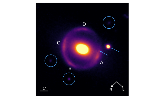
Figure 7: DESI-165.4754-06.0423 in HST WFC3 F140W. The four lensed images are labeled clockwise as A, B, C and D. To model this system, we mask out the light from three faint objects (circles) and the small object (solid arrow) in arc A (in projection). We also mask out the central region of the small nearby galaxy with a circular mask of radius 2.5 pixel (dashed arrow).

Table 2: Prior distribution used for lens modeling

Lens mass: $$\begin{cases}\hfill\theta_{E}&\sim\exp\left(\mathcal{N}(\ln 2.5,0.25\right)\\[1.0pt] \hfill\gamma&\sim\mathcal{TN}\left(2,0.25,1,2.7\right)\\[1.0pt] \hfill\epsilon_{1},\epsilon_{2}&\sim\mathcal{N}(0,0.1)\\[1.0pt] \hfill x,y&\sim\mathcal{N}(0,0.05)\\[1.0pt] \hfill\gamma_{ext,1},\gamma_{ext,2}&\sim\mathcal{N}(0,0.05)\end{cases}$$

Lens light: $$\begin{cases}\hfill R_{\text{l}}&{\color[rgb]{0,0,0}\sim\exp(\mathcal{N}(\ln 1,0.15))/\exp(\mathcal{N}({\ln 1,0.15}))}\\[1.0pt] \hfill n_{\text{l}}&{\color[rgb]{0,0,0}\sim\mathcal{U}(0.5,10)/\mathcal{U}(0.5,10)}\\[1.0pt] \hfill\epsilon_{\text{l},1},\epsilon_{\text{l},2}&{\color[rgb]{0,0,0}\sim\mathcal{N}(0,0.15)/\mathcal{N}(0,0.15)}\\[1.0pt] \hfill x_{\text{l}}&{\color[rgb]{0,0,0}\sim\mathcal{N}(0,0.05)/\mathcal{N}(0,0.10)}\\[1.0pt] \hfill y_{\text{l}}&{\color[rgb]{0,0,0}\sim\mathcal{N}(0,0.05)/\mathcal{N}(0,0.10)}\end{cases}$$

Source light: $$\begin{cases}\hfill R_{\text{s}}&\sim\exp\left(\mathcal{N}(\ln 0.25,0.15\right))\\[1.0pt] \hfill n_{\text{s}}&\sim\mathcal{U}(0.5,6)\\[1.0pt] \hfill\epsilon_{\text{s},1},\epsilon_{\text{s},2}&\sim\mathcal{N}(0,0.15)\\[1.0pt] \hfill x_{\text{s}},y_{\text{s}}&\sim\mathcal{N}(0,0.1)\\[1.0pt] \hfill\beta_{shp}&\sim\exp(\mathcal{N}(\ln 0.1,0.1))\\[1.0pt] \hfill x_{shp},y_{shp}&\sim\mathcal{N}(0,0.05)\end{cases}$$

Nearby galaxy: $$\begin{cases}\hfill R_{\text{g}}&{\color[rgb]{0,0,0}\sim\exp(\mathcal{N}(\ln 0.4,0.2))/\exp(\mathcal{N}({\ln 0.4,0.2}))}\\[1.0pt] \hfill n_{\text{g}}&{\color[rgb]{0,0,0}\sim\mathcal{U}(0.5,5)/\mathcal{U}(0.5,5)}\\[1.0pt] \hfill\epsilon_{\text{g},1},\epsilon_{\text{g},2}&{\color[rgb]{0,0,0}\sim\mathcal{TN}\left(0,0.15,-0.3,0.3\right)/\mathcal{TN}\left(0,0.15,-0.3,0.3\right)}\\[1.0pt] \hfill x_{\text{g}}&{\color[rgb]{0,0,0}\sim\mathcal{TN}(3.7,0.05,3.55,3.85)/\mathcal{TN}(3.7,0.05,3.55,3.85)}\\[1.0pt] \hfill y_{\text{g}}&{\color[rgb]{0,0,0}\sim\mathcal{TN}(0.25,0.05,0.1,0.4)/\mathcal{TN}(0.25,0.05,0.1,0.4)}\end{cases}$$

Notes — The mass model consists of EPL for the lens mass profile and external shear ($\gamma_{ext}$). $\theta_{E}$ is the Einstein radius in arcsec, while $\gamma$ defines the slope of the EPL profile. $x$ and $y$ are the mass center coordinates of the lens. $\gamma_{1,\text{ext}}$ and $\gamma_{2,\text{ext}}$ are the external shear components. The parameters $\epsilon_{1}$ and $\epsilon_{2}$ are the lens mass eccentricities. For the light model, subscripts $l$, $s$, $g$ indicate parameters belonging to the light profiles of the lens, the source, and the nearby galaxy, respectively. Thus $(\epsilon_{l,1}$, $\epsilon_{l,2})$, $(\epsilon_{s,1}$, $\epsilon_{s,2})$, $(\epsilon_{g,1}$, $\epsilon_{g,2})$ are the lens, source, and nearby galaxy light eccentricities, respectively. For the light of the lens and the nearby galaxy, we use two elliptical Sérsic profiles each, with their prior distributions separated with a slash. $R_{l}$, $R_{s},R_{g}$ are the half-light radii, and $n_{l}$, $n_{s},n_{g}$ are the Sérsic indices for the respective objects. $(x_{l},y_{l})$, $(x_{s},y_{s})$, $(x_{g},y_{g})$ describe their centers. The subscript $shp$ refers to the shapelets component for the source. Finally, $\mathcal{U}(a,b)$ indicates a uniform distribution with support $[a,b]$, $\mathcal{N}(\mu,\sigma)$ is a Gaussian with mean $\mu$ and standard deviation $\sigma$, and $\mathcal{TN}(\mu,\sigma,a,b)$ is a truncated Gaussian with support $[a,b]$.

We achieve excellent residuals (Figure 4). The best-fit parameters are shown in Tables 3 and 4. The sampling results for the lens and external shear mass parameters are shown in Figure 4. For this system, the marginal distributions of the SVI posterior match the HMC sampling results for some parameter pairs as well as they do for the simulated systems presented in Gu et al. (2022, their Figures 6 and A2), although the match is not as close for all pairs. Overall, the SVI posterior provides a good approximation to the HMC samples, demonstrating the efficacy of the SVI step. We determine the Einstein radius of the lens to be $\theta_{E}=2.646\pm 0.002^{\prime\prime}$ and the slope of the power law mass profile to be $\gamma=1.37\pm 0.02$. The total mass within the critical curve is $1.7390_{-0.0043}^{+0.0046}\times 10^{12}\,M_{\odot}$. We use the larger $R_{e}$ from the two Sérsic models as the effective light radius for the lensing galaxy, $1.89\pm 0.02^{\prime\prime}$, or $11.8\pm 0.1$ kpc, adopting the cosmological parameters from Planck Collaboration et al. (2020): $H_{0}$ = 67.4 $\pm$ 0.5 km s^-1 Mpc^-1, $\Omega_{\Lambda}$ = 0.6847 $\pm$ 0.0073, and $\Omega_{M}$ = 0.315 $\pm$ 0.007. The best-fit model predicts magnifications of $25.0\pm 1.6$, $59.0\pm 1.6$, $51.1\pm 2.7$, and $35.43\pm 0.79$ for images A, B, C, and D, respectively (Figure 4), computed as the average of the first and second methods in Appendix A.

As a further analysis on our best-fit $\gamma$, we explore regions higher than the prior for $\gamma$ in Table 2 ($\mathcal{TN}(2,0.25,1,2.7)$) and demonstrate stability in the other parameters and the consistent tendency for $\gamma$ to approach the lower boundary. We use two other priors for $\gamma$, while for all other parameters the prior remains unchanged. One is a truncated Gaussian distribution centered around $2.0$ with boundaries at $1.5$ and $2.5$. For the second, we use a uniform prior between $2.0$ and $3.0$. In both cases, the corner plot shows consistent values with our best-fit model for all parameters except for $\gamma$, whose posterior is pushing against the lower boundary, $1.5$ and $2.0$, respectively. In addition, we observe a $42.13\ \chi^{2}$ improvement for using the prior with the $1.5$ lower bound and a $551.87\ \chi^{2}$ improvement for using the prior with the $2.0$ lower bound, favoring our best-fit model in both cases.

Figure 8: From left to right, we show: the observed HST image (same orientation as in Figure 4), our best-fit model with critical curves in red, the reduced residual map, and the reconstruction of the unlensed source with caustics in green. Notice the presence of an inner critical curve and caustic due to the fact that $\gamma<2$.

Our sampling results are robust and statistically consistent using two widely employed metrics to measure the degree of convergence: the potential scale reduction factor (PSRF), often represented as $\hat{R}$ (Gelman & Rubin, 1992), and the effective sample size (ESS). In cosmological studies, these two criteria have been widely adopted (e.g., Krolewski et al., 2021; Douspis et al., 2022; Mandel et al., 2022; Rubin et al., 2023). An $\hat{R}$ that is close to 1 and a large ESS indicate that convergence to the same stationary distribution has been achieved. Gelman & Rubin (1992) suggested that an appropriate condition is $\hat{R}<1.2$.

For our best-fit model, the $\hat{R}$ values for all mass and light parameters of the lens and for all light parameters of the source are below 1.10. For the nearby galaxy light parameters, $\hat{R}$ is less than 1.12 and thus, all parameters are well below the threshold of $\hat{R}<1.2$. As for ESS, $\mathcal{O}(10^{3})$ is considered sufficiently high (e.g., Carpenter et al., 2017; Mandel et al., 2022). For our best-fit model, the minimum is 32,200, and the maximum, 40,000, demonstrating excellent sampling efficiency with very low autocorrelation (see, e.g., Gu et al., 2022).

In addition to being robust, our modeling approach is also fast. On a GPU node on the Perlmutter supercomputer at the National Energy Research Scientific Computing Center (NERSC), which has four A100 GPUs, the total execution time is 3 hrs. and 13 min. (193 min.), with the MAP, SVI, and HMC steps taking 1 hr. 9 min. (69 min.), 1 hr. 52 min. (112 min.), and 12 min., respectively. Considering that we take a fully forward modeling Bayesian approach with 41 model parameters for a highly nonlinear problem, this is remarkably fast.

Table 3: Best-fit mass parameters for DESI-165.4754-06.0423.

$\theta_{E}$	$\gamma$	$\epsilon_{1}$	$\epsilon_{2}$	$x$	$y$	$\gamma_{ext,1}$	$\gamma_{ext,2}$
$2.6463_{-0.0016}^{+0.0017}$	$1.372_{-0.022}^{+0.023}$	$0.1091_{-0.0020}^{+0.0020}$	$-0.1320_{-0.0020}^{+0.0020}$	$0.0272_{-0.0022}^{+0.0023}$	$-0.0018_{-0.0017}^{+0.0017}$	$0.0657_{-0.0024}^{+0.0024}$	$-0.0939_{-0.0022}^{+0.0022}$

Table 4: Best-fit light parameters for DESI-165.4754-06.0423.

Parameter	Lens light		Source light	Nearby galaxy light
$\bm{R_{e}}$	$0.4327_{-0.0050}^{+0.0051},$	$1.888_{-0.017}^{+0.017}$	$0.614^{+0.038}_{-0.036}$	$0.1353_{-0.0025}^{+0.0021},$	$0.227_{-0.065}^{+0.066}$
$\bm{n}$	$0.925_{-0.014}^{+0.014},$	$1.262_{-0.033}^{+0.035}$	$0.5050^{+0.0082}_{-0.0037}$	$0.523_{-0.017}^{+0.032},$	$3.86_{-1.22}^{+0.81}$
$\bm{\epsilon_{1}}$	$0.1350_{-0.0022}^{+0.0020},$	$0.1452_{-0.0012}^{+0.0012}$	$-0.058^{+0.025}_{-0.026}$	$0.0118_{-0.0089}^{+0.0087},$	$0.144_{-0.074}^{+0.059}$
$\bm{\epsilon_{2}}$	$-0.0577_{-0.0038}^{+0.0039},$	$-0.1832_{-0.0013}^{+0.0013}$	$0.192^{+0.023}_{-0.023}$	$-0.1124_{-0.0102}^{+0.0080},$	$0.264_{-0.055}^{+0.026}$
$\bm{x}$	$0.0042_{-0.0014}^{+0.0013},$	$0.0437_{-0.0023}^{+0.0024}$	$0.137^{+0.013}_{-0.012}$	$3.6100_{-0.0039}^{+0.0023},$	$3.7347_{-0.0079}^{+0.0062}$
$\bm{y}$	$0.0448_{-0.0012}^{+0.0013},$	$-0.0053_{-0.0018}^{+0.0018}$	$0.044^{+0.012}_{-0.012}$	$0.3704_{-0.0011}^{+0.0014},$	$0.3580_{-0.0058}^{+0.0043}$
$\bm{\beta_{shp}}$	-	-	$0.0505_{-0.0030}^{+0.0031}$	-	-
$\bm{x_{shp}}$	-	-	$-0.0249_{-0.0040}^{+0.0039}$	-	-
$\bm{y_{shp}}$	-	-	$0.0354_{-0.0025}^{+0.0025}$	-	-

Notes — We model the light of both the lens and nearby galaxy with two elliptical Sérsic profiles each, with the best-fit parameters shown in the second and last main columns, respectively.

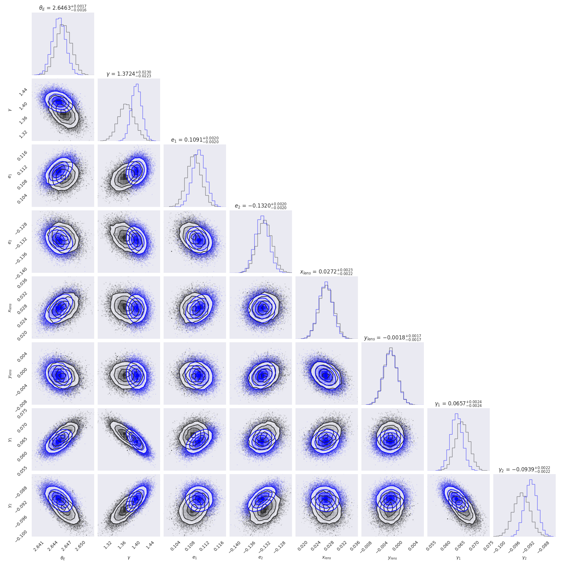
Figure 9: The corner plot showing our sampling results for the lens and external shear mass parameters, with SVI and HMC samples shown in blue and black, respectively.

5 Discussion

The accurate measurements of the density slopes of lensing galaxies, which are typically elliptical galaxies, have significant implications for time-delay $H_{0}$ constraints (e.g., Birrer et al., 2020) and are crucial for determining other cosmological parameters using a large number of static lenses (e.g., Li et al., 2024). Such measurements for lensing systems over a wide range of redshifts also makes it possible to study the structural evolution of massive elliptical galaxies (e.g., Sahu et al., 2024).

Numerical simulations of cold dark matter (CDM) halos predict mass profiles with a logarithmic slope approaching $\gamma=1$ and 3 at small and large radii, respectively (e.g., Navarro et al., 1996, NFW). In cluster strong lenses, low $\gamma$ values near the cluster center certainly have been measured (e.g., Broadhurst et al., 2000, at 1.26). For galaxy-scale lenses, with significant baryon contribution (typically stellar in elliptical galaxies) to the mass, the picture is more complicated. Nevertheless, low $\gamma$ values around 1.4 have also been reported, for five systems from the BELLS and SL2S samples (Li et al., 2018) and one from the LSD sample (Treu & Koopmans, 2004). There is an even larger number of systems (three from SLACS and six from BELLS) for which the $\gamma$ value is consistent with our best-fit value for DESI-165.4754-06.0423 to within 2$\sigma$. As mentioned earlier, this system appears to be at the center of a galaxy group, and such systems have not been as extensively studied compared with galaxy-scale strong lenses that typically have smaller Einstein radii. In addition, the previous analyses on the LSD, SLACS, BELLS, and SL2S samples were not performed with a fully forward modeling approach, nor have convergence metrics been applied to those results. Thus applying this approach consistently to a large number of systems with satisfactory sampling convergence for each system (see § 4 and the paragraph below) can shed more light on the mass slope question. Finally, for this system, comparison with mass profile modeling based on well-measured velocity dispersion, especially from spatially resolved stellar dynamics (e.g., Treu & Koopmans, 2004; Barnabè et al., 2009; Shajib et al., 2023; Turner et al., 2024) will be very interesting and is left for a future investigation.

Given the covariance that exists between the fitting parameters of a model, to properly estimate the uncertainties of these parameters, it is best to perform full forward modeling. However, to take this approach for strong lensing is challenging given that it is inherently a highly nonlinear problem (in fact, the solution is near a mathematical singularity, the critical curve). Using high resolution data (e.g., HST) for lens modeling would require a high dimensional parameter space and, if the Einstein radius is large (which is the case for this system), a large cutout—both will present even greater challenges. Thanks to modern GPUs and automatic differentiation, this became possible in recent years and we developed GIGA-Lens. In this pipeline, we also assess convergence for statistical inference, using the metrics of $\hat{R}$ and ESS. We show that for this system we have achieved excellent convergence. Thus this first attempt has yielded very encouraging results.

In the event of a SN in the source galaxy, the precise time-delays will depend on the location of the SN. From using different test locations, the arrival time offset between the earliest and latest images is $\gtrsim 40$ days, which would be ideal for $H_{0}$ measurements. We will determine the stellar mass and star formation rates to estimate the SN rates, based on the photometric and spectroscopic data for this and other systems in follow-up analyses. Finally, from this modeling effort, we do not see evidence for dark matter substructure or line-of-sight low-mass halos in this system. In future publications, we will report the modeling results for other systems in this program, including the detection status of substructure/low-mass LOS halos.

6 Conclusion

In this paper—Paper I of the DESI Strong Lens Foundry series—we present our Hubble Space Telescope SNAP program (GO-15867, PI: Huang) for confirming strong gravitational lens candidates found using Residual Neural Networks in the DESI Legacy Imaging Surveys. It is the first HST program to follow up on strong lens candidates found using machine learning in imaging surveys. All 51 systems observed by HST were confirmed to be lenses. To our knowledge, this is the first time an HST SNAP program for strong lens confirmation has achieved a 100% success rate.

Spectroscopic observations of these systems are ongoing through DESI (Paper II in this series; Huang, Inchausti et al., in prep) and on Keck NIRES (Paper III in this series, Agarwal et al. in prep).

We have applied a fully forward modeling Bayesian approach (GIGA-Lens) using multiple GPUs, for the first time in both regards, to a real gravitational lensing system with HST (or any high resolution) data, DESI-165.4754-06.0423. The Einstein radius of the lens is $\theta_{E}=2.646\pm 0.002^{\prime\prime}$ and the slope of the power law mass profile is $\gamma=1.37\pm 0.02$. We report excellent sampling results: for all parameters the $\hat{R}$ is well-below the threshold of 1.2 (based on the TensorFlow definition and implementation; see Footnote12) and the effective sample size (ESS), greater than 37,000. Our model is also fast. For such a complex model (41 parameters) for a highly nonlinear problem, with a large HST image size ($128^{2}$ pixels), the time it takes to run GIGA-Lens is ${{3\leavevmode\nobreak\ \rm{hrs.}13\leavevmode\nobreak\ \rm{min.}}}$ on four A100 GPU on one GPU node on the Perlmutter supercomputer at NERSC. With further improvement in the hardware and software almost a certainty, this concretely demonstrates a promising future of modeling many more strong lensing systems with HST data, or observed with comparable or superior image resolution and depth (e.g., Euclid, the James Webb Space Telescope, and the Nancy Grace Roman Space Telescope), with speed and statistical rigor.

Recently two cluster lensed SNe have been used to determine $H_{0}$ (Kelly et al., 2023; Pascale et al., 2024), with a measurement from a third system possible (Pierel et al., 2023). For the two resolved galaxy-scale strongly lensed SNe discovered so far, the Einstein radii ($\theta_{E}$), and therefore time-delays ($<1$ day), are too small for this to be possible (Mörtsell et al., 2020; Goobar et al., 2023; Pierel et al., 2023). However, with the much larger sample of galaxy-scale strong lenses already observed with high resolution imaging and modeled, with a time-varying source (e.g., Suyu et al., 2010, 2013; Wong et al., 2019; Shajib et al., 2023; Schmidt et al., 2023) or without (e.g., Bolton et al., 2008; Shu et al., 2016a), there are still significant advantages of using galaxy-scale lensed SNe for $H_{0}$ measurement: the modeling is simpler and the systematics are well-understood (e.g., Kochanek, 2020; Birrer et al., 2020; Shajib et al., 2023). From the ongoing work of modeling the galaxy-scale strong lenses in this program beyond the system presented in this work, we will measure the lens mass slope over a wide redshift range, providing robust prior for not only $H_{0}$ measurements, but the determination of other cosmological parameters (e.g., Li et al., 2024). In addition, building on the experience we have gained using GIGA-Lens from modeling systems in this sample, we have extended this framework to lensed point sources (e.g., SNe; S. Baltasar, N. Ratier-Werbin & X. Huang in prep). Finally, this framework has also been extended to model group/cluster scale lenses (Urcelay et al., 2025), which we will apply to the group/cluster strong lenses in this sample.

Appendix A Magnification

This appendix describes the magnification calculations for the lensed arcs. We will show three independent methods that provide consistent results with each other.

In the first method, we choose a reasonable luminosity threshold for the source light. The pixels in the source plane and the lens plane with values exceeding the threshold are selected, with both images being non-PSF convolved. This threshold is chosen in a manner that allows each arc to be isolated from the others. The ratios between the number of pixels of each arc and the number of pixels of the source, above this threshold, will be the magnifications. In practice, an important adjustment needs be made in order to achieve accurate results. Each flux value in the image plane comes from a corresponding pixel in the source plane. GIGA-Lens ensures this correspondence by ray-tracing each pixel of the image plane to the source plane. It then assigns the pixel in the image plane with the value of the corresponding pixel on the source plane. However, for magnified images, using a grid in the source plane that is the same as the lens plane can lead to inaccuracy in the magnification calculation. Such a grid proves to be too coarse and thus leads to an underestimation of the magnification. We use the peak pixel values in the source and image planes as a diagnostic. We find that the source plane grid is sufficiently fine if a correspondence between the peak pixel values in the image and source planes can be established. We thus proceed as follows. Let $\delta_{I}$ and $\delta_{S}$ be the pixel sizes, measured in arcseconds, of the image and source planes, respectively, with a sufficiently small $\delta_{S}$ (for typical lensed images, which are magnified, $\delta_{I}>\delta_{S}$). In the case of DESI-165.4754-06.0423, we use $\delta_{I}=0.065^{\prime\prime}$ and $\delta_{S}=0.02^{\prime\prime}$. We can now count pixels and compute the ratio for each arc. We account for the pixel size difference between the planes by multiplying the ratio by the factor $(\delta_{I}/\delta_{S})^{2}$. This is the magnification. This method is straightforward, but it requires determining a reasonable grid resolution for the source plane.

We now introduce a second method that does not require that we choose an appropriate resolution in the source plane. For each pixel that exceeds a chosen threshold (identical to the one used in the first method) within a non-PSF-convolved arc, we ray-trace the center of that pixel to the source plane. We then compute the area of the convex hull that encloses these delensed points. The magnification is the ratio between the area of each arc and the source area calculated this way, as long as source structure does not have concave features and the convex hull results in a reasonable enclosure.

As a final check, we apply the point-wise magnification function from Lenstronomy to our model. The mean values of all points within each arc are also consistent with the magnification for each arc calculated using the first two methods. We present the magnification results for these three methods in Table 5.

In the literature, magnifications are typically calculated using one method. Here we take three reasonable approaches, and we note that the differences in the magnifications from using these different methods are greater than the statistical uncertainties. Thus, we regard the differences between the methods as an estimate for the uncertainty. For all three methods, the magnification for all four lensed images are in agreement to $\lesssim 10\%$. We take the averages of the first two methods as the magnifications and their differences divided by two as the uncertainty. This is what is reported in the main text. We treat the third method as a “sanity check”.

Table 5: Magnification calculations for DESI-165.4754-06.0423.

Method	$A$	$B$	$C$	$D$	Total
$1^{\text{st}}$	$26.65$	$57.33$	$53.81$	$36.21$	$174.00$
$2^{\text{nd}}$	$23.41$	$60.61$	$48.43$	$34.64$	$167.09$
$3^{\text{rd}}$	$24.83$	$57.15$	$53.06$	$34.95$	$169.99$

Note. — Our magnification calculations, using three approaches, for images A, B, C, D (see Figure 4), and the total magnification, respectively.

References

- Abadi et al. (2015) Abadi, M., Agarwal, A., Barham, P., et al. 2015, TensorFlow: Large-Scale Machine Learning on Heterogeneous Systems. https://www.tensorflow.org/
- Abbott et al. (2017) Abbott, B. P., Abbott, R., Abbott, T. D., et al. 2017, Nature, 551, 85, doi: 10.1038/nature24471
- Abbott et al. (2018a) Abbott, T. M. C., Abdalla, F. B., Annis, J., et al. 2018a, MNRAS, 480, 3879, doi: 10.1093/mnras/sty1939
- Abbott et al. (2018b) Abbott, T. M. C., Abdalla, F. B., Allam, S., et al. 2018b, ApJS, 239, 18, doi: 10.3847/1538-4365/aae9f0
- Adame et al. (2024) Adame, A. G., Aguilar, J., Ahlen, S., et al. 2024, The Astronomical Journal, 168, 58, doi: 10.3847/1538-3881/ad3217
- Astropy Collaboration et al. (2022) Astropy Collaboration, Price-Whelan, A. M., Lim, P. L., et al. 2022, ApJ, 935, 167, doi: 10.3847/1538-4357/ac7c74
- Barnabè et al. (2009) Barnabè, M., Czoske, O., Koopmans, L. V. E., et al. 2009, MNRAS, 399, 21, doi: 10.1111/j.1365-2966.2009.14941.x
- Birrer & Amara (2018) Birrer, S., & Amara, A. 2018, Physics of the Dark Universe, 22, 189, doi: 10.1016/j.dark.2018.11.002
- Birrer et al. (2015) Birrer, S., Amara, A., & Refregier, A. 2015, ApJ, 813, 102, doi: 10.1088/0004-637X/813/2/102
- Birrer et al. (2020) Birrer, S., Shajib, A. J., Galan, A., et al. 2020, Astronomy & Astrophysics, 643, A165, doi: 10.1051/0004-6361/202038861
- Birrer et al. (2021) Birrer, S., Shajib, A., Gilman, D., et al. 2021, The Journal of Open Source Software, 6, 3283, doi: 10.21105/joss.03283
- Blandford & Narayan (1992) Blandford, R. D., & Narayan, R. 1992, ARA&A, 30, 311, doi: 10.1146/annurev.astro.30.1.311
- Bolamperti et al. (2024) Bolamperti, A., Grillo, C., Caminha, G. B., et al. 2024, arXiv e-prints, arXiv:2411.07289, doi: 10.48550/arXiv.2411.07289
- Bolton et al. (2008) Bolton, A. S., Burles, S., Koopmans, L. V. E., et al. 2008, ApJ, 682, 964, doi: 10.1086/589327
- Bolton et al. (2006) Bolton, A. S., Burles, S., Koopmans, L. V. E., Treu, T., & Moustakas, L. A. 2006, ApJ, 638, 703, doi: 10.1086/498884
- Bolton et al. (2012) Bolton, A. S., Brownstein, J. R., Kochanek, C. S., et al. 2012, ApJ, 757, 82, doi: 10.1088/0004-637X/757/1/82
- Bradač et al. (2008) Bradač, M., Allen, S. W., Treu, T., et al. 2008, ApJ, 687, 959–967, doi: 10.1086/591246
- Bradbury et al. (2018) Bradbury, J., Frostig, R., Hawkins, P., et al. 2018, JAX: composable transformations of Python+NumPy programs, 0.2.5. http://github.com/google/jax
- Bradley et al. (2023) Bradley, L., Sipőcz, B., Robitaille, T., et al. 2023, astropy/photutils: 1.8.0, 1.8.0, Zenodo, doi: 10.5281/zenodo.7946442
- Broadhurst et al. (2000) Broadhurst, T., Huang, X., Frye, B., & Ellis, R. 2000, ApJ, 534, L15, doi: 10.1086/312651
- Carpenter et al. (2017) Carpenter, B., Gelman, A., Hoffman, M. D., et al. 2017, Journal of Statistical Software, 76, 1–32, doi: 10.18637/jss.v076.i01
- Cañameras, R. et al. (2020) Cañameras, R., Schuldt, S., Suyu, S. H., et al. 2020, A&A, 644, A163, doi: 10.1051/0004-6361/202038219
- Çaǧan Şengül et al. (2022) Çaǧan Şengül, A. Ç., Dvorkin, C., Ostdiek, B., & Tsang, A. 2022, MNRAS, 515, 4391, doi: 10.1093/mnras/stac1967
- Chen et al. (2022) Chen, W., Kelly, P. L., Oguri, M., et al. 2022, Nature, 611, 256, doi: 10.1038/s41586-022-05252-5
- Chevallier & Polarski (2001) Chevallier, M., & Polarski, D. 2001, International Journal of Modern Physics D, 10, 213, doi: 10.1142/S0218271801000822
- Choi et al. (2020) Choi, S. K., Hasselfield, M., Ho, S.-P. P., et al. 2020, Journal of Cosmology and Astroparticle Physics, 2020, 045–045, doi: 10.1088/1475-7516/2020/12/045
- Cikota et al. (2023) Cikota, A., Bertolla, I. T., Huang, X., et al. 2023, ApJ, 953, L5, doi: 10.3847/2041-8213/ace9da
- Clowe et al. (2006) Clowe, D., Bradač, M., Gonzalez, A. H., et al. 2006, ApJ, 648, L109, doi: 10.1086/508162
- Collett & Auger (2014) Collett, T. E., & Auger, M. W. 2014, MNRAS, 443, 969, doi: 10.1093/mnras/stu1190
- Collett et al. (2012) Collett, T. E., Auger, M. W., Belokurov, V., Marshall, P. J., & Hall, A. C. 2012, MNRAS, 424, 2864, doi: 10.1111/j.1365-2966.2012.21424.x
- Collett et al. (2018) Collett, T. E., Oldham, L. J., Smith, R. J., et al. 2018, Science, 360, 1342, doi: 10.1126/science.aao2469
- Dai et al. (2020) Dai, L., Kaurov, A. A., Sharon, K., et al. 2020, MNRAS, 495, 3192, doi: 10.1093/mnras/staa1355
- Dawes et al. (2023) Dawes, C., Storfer, C., Huang, X., et al. 2023, The Astrophysical Journal Supplement Series, 269, 61, doi: 10.3847/1538-4365/ad015a
- Dawson et al. (2016) Dawson, K. S., Kneib, J.-P., Percival, W. J., et al. 2016, AJ, 151, 44, doi: 10.3847/0004-6256/151/2/44
- DESI Collaboration et al. (2016a) DESI Collaboration, Aghamousa, A., Aguilar, J., et al. 2016a, arXiv e-prints, arXiv:1611.00036, doi: 10.48550/arXiv.1611.00036
- DESI Collaboration et al. (2016b) —. 2016b, arXiv e-prints, arXiv:1611.00037, doi: 10.48550/arXiv.1611.00037
- Dey et al. (2016) Dey, A., Rabinowitz, D., Karcher, A., et al. 2016, in Proc. SPIE, Vol. 9908, Ground-based and Airborne Instrumentation for Astronomy VI, 99082C, doi: 10.1117/12.2231488
- Dey et al. (2019) Dey, A., Schlegel, D. J., Lang, D., et al. 2019, AJ, 157, 168, doi: 10.3847/1538-3881/ab089d
- Dhawan et al. (2023) Dhawan, S., Thorp, S., Mandel, K. S., et al. 2023, MNRAS, 524, 235, doi: 10.1093/mnras/stad1590
- Diaz Rivero & Dvorkin (2020) Diaz Rivero, A., & Dvorkin, C. 2020, Phys. Rev. D, 101, 023515, doi: 10.1103/PhysRevD.101.023515
- Dillon et al. (2017) Dillon, J. V., Langmore, I., Tran, D., et al. 2017, TensorFlow Distributions. https://arxiv.org/abs/1711.10604
- Douspis et al. (2022) Douspis, M., Salvati, L., Gorce, A., & Aghanim, N. 2022, A&A, 659, A99, doi: 10.1051/0004-6361/202142004
- Dux et al. (2024) Dux, F., Millon, M., Lemon, C., et al. 2024, arXiv e-prints, arXiv:2411.04177, doi: 10.48550/arXiv.2411.04177
- Filipp et al. (2023) Filipp, A., Shu, Y., Pakmor, R., Suyu, S. H., & Huang, X. 2023, A&A, 677, A113, doi: 10.1051/0004-6361/202346594
- Flaugher et al. (2015) Flaugher, B., Diehl, H. T., Honscheid, K., et al. 2015, AJ, 150, 150, doi: 10.1088/0004-6256/150/5/150
- Foreman-Mackey (2016) Foreman-Mackey, D. 2016, The Journal of Open Source Software, 1, 24, doi: 10.21105/joss.00024
- Freedman et al. (2019) Freedman, W. L., Madore, B. F., Hatt, D., et al. 2019, ApJ, 882, 34, doi: 10.3847/1538-4357/ab2f73
- Freedman et al. (2020) Freedman, W. L., Madore, B. F., Hoyt, T., et al. 2020, ApJ, 891, 57, doi: 10.3847/1538-4357/ab7339
- Frye et al. (2024) Frye, B. L., Pascale, M., Pierel, J., et al. 2024, The Astrophysical Journal, 961, 171, doi: 10.3847/1538-4357/ad1034
- Gelman et al. (2014) Gelman, A., Carlin, J. B., Stern, H. S., et al. 2014, Bayesian Data Analysis (CRC Press)
- Gelman & Rubin (1992) Gelman, A., & Rubin, D. B. 1992, Statistical Science, 7, 457 , doi: 10.1214/ss/1177011136
- Goldstein & Nugent (2017) Goldstein, D. A., & Nugent, P. E. 2017, ApJ, 834, L5, doi: 10.3847/2041-8213/834/1/L5
- Goldstein et al. (2019) Goldstein, D. A., Nugent, P. E., & Goobar, A. 2019, The Astrophysical Journal Supplement Series, 243, 6, doi: 10.3847/1538-4365/ab1fe0
- Goldstein et al. (2018) Goldstein, D. A., Nugent, P. E., Kasen, D. N., & Collett, T. E. 2018, ApJ, 855, 22, doi: 10.3847/1538-4357/aaa975
- Goobar et al. (2017) Goobar, A., Amanullah, R., Kulkarni, S. R., et al. 2017, Science, 356, 291, doi: 10.1126/science.aal2729
- Goobar et al. (2023) Goobar, A., Johansson, J., Schulze, S., et al. 2023, Nature Astronomy, 7, 1137, doi: 10.1038/s41550-023-02034-5
- Gu et al. (2022) Gu, A., Huang, X., Sheu, W., et al. 2022, ApJ, 935, 49, doi: 10.3847/1538-4357/ac6de4
- Harris et al. (2020) Harris, C. R., Millman, K. J., van der Walt, S. J., et al. 2020, Nature, 585, 357, doi: 10.1038/s41586-020-2649-2
- Hessel et al. (2020) Hessel, M., Budden, D., Viola, F., et al. 2020, Optax: composable gradient transformation and optimisation, in JAX!, 0.0.1. http://github.com/deepmind/optax
- Hezaveh et al. (2016) Hezaveh, Y. D., Dalal, N., Marrone, D. P., et al. 2016, ApJ, 823, 37, doi: 10.3847/0004-637X/823/1/37
- Huang et al. (2009) Huang, X., Morokuma, T., Fakhouri, H. K., et al. 2009, ApJ, 707, L12, doi: 10.1088/0004-637X/707/1/L12
- Huang et al. (2020) Huang, X., Storfer, C., Ravi, V., et al. 2020, The Astrophysical Journal, 894, 78, doi: 10.3847/1538-4357/ab7ffb
- Huang et al. (2021) Huang, X., Storfer, C., Gu, A., et al. 2021, ApJ, 909, 27, doi: 10.3847/1538-4357/abd62b
- Hunter (2007) Hunter, J. D. 2007, Computing in Science & Engineering, 9, 90, doi: 10.1109/MCSE.2007.55
- Jacobs et al. (2017) Jacobs, C., Glazebrook, K., Collett, T., More, A., & McCarthy, C. 2017, MNRAS, 471, 167, doi: 10.1093/mnras/stx1492
- Jacobs et al. (2019a) Jacobs, C., Collett, T., Glazebrook, K., et al. 2019a, MNRAS, 484, 5330, doi: 10.1093/mnras/stz272
- Jacobs et al. (2019b) —. 2019b, ApJS, 243, 17, doi: 10.3847/1538-4365/ab26b6
- Jauzac et al. (2018) Jauzac, M., Harvey, D., & Massey, R. 2018, MNRAS, 477, 4046, doi: 10.1093/mnras/sty909
- Jullo et al. (2010) Jullo, E., Natarajan, P., Kneib, J. P., et al. 2010, Science, 329, 924, doi: 10.1126/science.1185759
- Kelly et al. (2015) Kelly, P. L., Filippenko, A. V., Burke, D. L., et al. 2015, Science, 347, 1459, doi: 10.1126/science.1261475
- Kelly et al. (2023) Kelly, P. L., Rodney, S., Treu, T., et al. 2023, ApJ, 948, 93, doi: 10.3847/1538-4357/ac4ccb
- Khetan et al. (2021) Khetan, N., Izzo, L., Branchesi, M., et al. 2021, Astronomy & Astrophysics, 647, A72, doi: 10.1051/0004-6361/202039196
- Kochanek (1991) Kochanek, C. S. 1991, ApJ, 373, 354, doi: 10.1086/170057
- Kochanek (2020) —. 2020, MNRAS, 493, 1725, doi: 10.1093/mnras/staa344
- Koopmans & Treu (2002) Koopmans, L. V. E., & Treu, T. 2002, ApJ, 568, L5, doi: 10.1086/340143
- Koopmans et al. (2006) Koopmans, L. V. E., Treu, T., Bolton, A. S., Burles, S., & Moustakas, L. A. 2006, ApJ, 649, 599, doi: 10.1086/505696
- Krolewski et al. (2021) Krolewski, A., Ferraro, S., & White, M. 2021, J. Cosmology Astropart. Phys, 2021, 028, doi: 10.1088/1475-7516/2021/12/028
- Lanusse et al. (2018) Lanusse, F., Ma, Q., Li, N., et al. 2018, MNRAS, 473, 3895, doi: 10.1093/mnras/stx1665
- Lewis et al. (2002) Lewis, G. F., Carilli, C., Papadopoulos, P., & Ivison, R. J. 2002, MNRAS, 330, L15, doi: 10.1046/j.1365-8711.2002.05260.x
- Li et al. (2018) Li, R., Shu, Y., & Wang, J. 2018, MNRAS, 480, 431, doi: 10.1093/mnras/sty1813
- Li et al. (2020) Li, R., Napolitano, N. R., Tortora, C., et al. 2020, ApJ, 899, 30, doi: 10.3847/1538-4357/ab9dfa
- Li et al. (2024) Li, T., Collett, T. E., Krawczyk, C. M., & Enzi, W. 2024, MNRAS, 527, 5311, doi: 10.1093/mnras/stad3514
- Linder (2003) Linder, E. V. 2003, Phys. Rev. Lett., 90, 091301, doi: 10.1103/PhysRevLett.90.091301
- Linder (2011) —. 2011, Phys. Rev. D, 84, 123529, doi: 10.1103/PhysRevD.84.123529
- Linder (2016) —. 2016, Phys. Rev. D, 94, 083510, doi: 10.1103/PhysRevD.94.083510
- Magee et al. (2023) Magee, M. R., Sainz de Murieta, A., Collett, T. E., & Enzi, W. 2023, MNRAS, 525, 542, doi: 10.1093/mnras/stad2263
- Mandel et al. (2022) Mandel, K. S., Thorp, S., Narayan, G., Friedman, A. S., & Avelino, A. 2022, MNRAS, 510, 3939, doi: 10.1093/mnras/stab3496
- Meneghetti et al. (2020) Meneghetti, M., Davoli, G., Bergamini, P., et al. 2020, Science, 369, 1347, doi: 10.1126/science.aax5164
- Monna et al. (2017) Monna, A., Seitz, S., Balestra, I., et al. 2017, MNRAS, 466, 4094, doi: 10.1093/mnras/stx015
- More et al. (2012) More, A., Cabanac, R., More, S., et al. 2012, ApJ, 749, 38, doi: 10.1088/0004-637X/749/1/38
- Mörtsell et al. (2020) Mörtsell, E., Johansson, J., Dhawan, S., et al. 2020, MNRAS, 496, 3270, doi: 10.1093/mnras/staa1600
- Navarro et al. (1996) Navarro, J. F., Frenk, C. S., & White, S. D. M. 1996, ApJ, 462, 563, doi: 10.1086/177173
- Nierenberg et al. (2023) Nierenberg, A. M., Keeley, R. E., Sluse, D., et al. 2023, arXiv e-prints, arXiv:2309.10101, doi: 10.48550/arXiv.2309.10101
- Oguri & Marshall (2010) Oguri, M., & Marshall, P. J. 2010, MNRAS, 405, 2579, doi: 10.1111/j.1365-2966.2010.16639.x
- Pascale et al. (2024) Pascale, M., Frye, B. L., Pierel, J. D. R., et al. 2024, arXiv, doi: 10.48550/arxiv.2403.18902
- Peng et al. (2010) Peng, C. Y., Ho, L. C., Impey, C. D., & Rix, H.-W. 2010, The Astronomical Journal, 139, 2097, doi: 10.1088/0004-6256/139/6/2097
- Petrillo et al. (2017) Petrillo, C. E., Tortora, C., Chatterjee, S., et al. 2017, MNRAS, 472, 1129, doi: 10.1093/mnras/stx2052
- Petrillo et al. (2019) Petrillo, C. E., Tortora, C., Vernardos, G., et al. 2019, MNRAS, 484, 3879, doi: 10.1093/mnras/stz189
- Philcox et al. (2021) Philcox, O. H., Sherwin, B. D., Farren, G. S., & Baxter, E. J. 2021, Physical Review D, 103, doi: 10.1103/physrevd.103.023538
- Pierel & Rodney (2019) Pierel, J. D. R., & Rodney, S. 2019, ApJ, 876, 107, doi: 10.3847/1538-4357/ab164a
- Pierel et al. (2021) Pierel, J. D. R., Rodney, S., Vernardos, G., et al. 2021, ApJ, 908, 190, doi: 10.3847/1538-4357/abd8d3
- Pierel et al. (2023) Pierel, J. D. R., Arendse, N., Ertl, S., et al. 2023, ApJ, 948, 115, doi: 10.3847/1538-4357/acc7a6
- Planck Collaboration et al. (2020) Planck Collaboration, Aghanim, N., Akrami, Y., et al. 2020, A&A, 641, A6, doi: 10.1051/0004-6361/201833910
- Quimby et al. (2014) Quimby, R. M., Oguri, M., More, A., et al. 2014, Science, 344, 396, doi: 10.1126/science.1250903
- Refsdal (1964) Refsdal, S. 1964, MNRAS, 128, 307, doi: 10.1093/mnras/128.4.307
- Riess et al. (2019) Riess, A. G., Casertano, S., Yuan, W., Macri, L. M., & Scolnic, D. 2019, ApJ, 876, 85, doi: 10.3847/1538-4357/ab1422
- Ritondale et al. (2019) Ritondale, E., Vegetti, S., Despali, G., et al. 2019, MNRAS, 485, 2179, doi: 10.1093/mnras/stz464
- Rodney et al. (2021) Rodney, S. A., Brammer, G. B., Pierel, J. D. R., et al. 2021, Nature Astronomy, 5, 1118, doi: 10.1038/s41550-021-01450-9
- Rodney et al. (2016) Rodney, S. A., Strolger, L. G., Kelly, P. L., et al. 2016, ApJ, 820, 50, doi: 10.3847/0004-637X/820/1/50
- Rubin et al. (2023) Rubin, D., Aldering, G., Betoule, M., et al. 2023, arXiv e-prints, arXiv:2311.12098, doi: 10.48550/arXiv.2311.12098
- Sahu et al. (2024) Sahu, N., Tran, K.-V., Suyu, S. H., et al. 2024, ApJ, 970, 86, doi: 10.3847/1538-4357/ad4ce3
- Schmidt et al. (2023) Schmidt, T., Treu, T., Birrer, S., et al. 2023, MNRAS, 518, 1260, doi: 10.1093/mnras/stac2235
- Sérsic (1963) Sérsic, J. L. 1963, Boletin de la Asociacion Argentina de Astronomia La Plata Argentina, 6, 41
- Shajib et al. (2021) Shajib, A. J., Treu, T., Birrer, S., & Sonnenfeld, A. 2021, MNRAS, 503, 2380, doi: 10.1093/mnras/stab536
- Shajib et al. (2019) Shajib, A. J., Birrer, S., Treu, T., et al. 2019, MNRAS, 483, 5649, doi: 10.1093/mnras/sty3397
- Shajib et al. (2023) Shajib, A. J., Mozumdar, P., Chen, G. C. F., et al. 2023, A&A, 673, A9, doi: 10.1051/0004-6361/202345878
- Sharma et al. (2023) Sharma, D., Collett, T. E., & Linder, E. V. 2023, J. Cosmology Astropart. Phys, 2023, 001, doi: 10.1088/1475-7516/2023/04/001
- Sharma & Linder (2022) Sharma, D., & Linder, E. V. 2022, Journal of Cosmology and Astroparticle Physics, 2022, 033, doi: 10.1088/1475-7516/2022/07/033
- Sheu et al. (2023) Sheu, W., Huang, X., Cikota, A., et al. 2023, ApJ, 952, 10, doi: 10.3847/1538-4357/acd1e4
- Sheu et al. (2024) Sheu, W., Cikota, A., Huang, X., et al. 2024, ApJ, 973, 3, doi: 10.3847/1538-4357/ad65d3
- Shu et al. (2018) Shu, Y., Bolton, A. S., Mao, S., et al. 2018, ApJ, 864, 91, doi: 10.3847/1538-4357/aad5ea
- Shu et al. (2021) Shu, Y., Bolton, A. S., Mao, S., et al. 2021, The Astrophysical Journal, 919, 67, doi: 10.3847/1538-4357/ac24a4
- Shu et al. (2016a) Shu, Y., Bolton, A. S., Moustakas, L. A., et al. 2016a, ApJ, 820, 43, doi: 10.3847/0004-637X/820/1/43
- Shu et al. (2016b) Shu, Y., Bolton, A. S., Kochanek, C. S., et al. 2016b, ApJ, 824, 86, doi: 10.3847/0004-637X/824/2/86
- Sonnenfeld et al. (2013) Sonnenfeld, A., Treu, T., Gavazzi, R., et al. 2013, ApJ, 777, 98, doi: 10.1088/0004-637X/777/2/98
- Storfer et al. (2024) Storfer, C., Huang, X., Gu, A., et al. 2024, The Astrophysical Journal Supplement Series, 274, 16, doi: 10.3847/1538-4365/ad527e
- Suyu et al. (2024) Suyu, S. H., Goobar, A., Collett, T., More, A., & Vernardos, G. 2024, Space Science Reviews, 220, doi: 10.1007/s11214-024-01044-7
- Suyu et al. (2010) Suyu, S. H., Marshall, P. J., Auger, M. W., et al. 2010, ApJ, 711, 201, doi: 10.1088/0004-637X/711/1/201
- Suyu et al. (2013) Suyu, S. H., Auger, M. W., Hilbert, S., et al. 2013, ApJ, 766, 70, doi: 10.1088/0004-637X/766/2/70
- Suyu et al. (2020) Suyu, S. H., Huber, S., Cañameras, R., et al. 2020, Astronomy & Astrophysics, 644, A162, doi: 10.1051/0004-6361/202037757
- Talbot et al. (2021) Talbot, M. S., Brownstein, J. R., Dawson, K. S., Kneib, J.-P., & Bautista, J. 2021, MNRAS, 502, 4617, doi: 10.1093/mnras/stab267
- Tessore et al. (2016) Tessore, N., Bellagamba, F., & Metcalf, R. B. 2016, MNRAS, 463, 3115, doi: 10.1093/mnras/stw2212
- Tessore & Metcalf (2015) Tessore, N., & Metcalf, R. B. 2015, A&A, 580, A79, doi: 10.1051/0004-6361/201526773
- The Dark Energy Survey Collaboration (2005) The Dark Energy Survey Collaboration. 2005, arXiv e-prints, astro. https://arxiv.org/abs/astro-ph/0510346
- Treu (2010) Treu, T. 2010, ARA&A, 48, 87, doi: 10.1146/annurev-astro-081309-130924
- Treu & Koopmans (2004) Treu, T., & Koopmans, L. V. E. 2004, ApJ, 611, 739, doi: 10.1086/422245
- Treu & Marshall (2016) Treu, T., & Marshall, P. J. 2016, Astronomy and Astrophysics Review, 24, 11, doi: 10.1007/s00159-016-0096-8
- Turner et al. (2024) Turner, H. C., Smith, R. J., & Collett, T. E. 2024, MNRAS, 528, 3559, doi: 10.1093/mnras/stae263
- Urcelay et al. (2025) Urcelay, F., Jullo, E., Barrientos, L. F., Huang, X., & Hernandez, J. 2025, A&A, 694, A35, doi: 10.1051/0004-6361/202449261
- Vegetti et al. (2018) Vegetti, S., Despali, G., Lovell, M. R., & Enzi, W. 2018, MNRAS, 481, 3661, doi: 10.1093/mnras/sty2393
- Vegetti & Koopmans (2009) Vegetti, S., & Koopmans, L. V. E. 2009, MNRAS, 400, 1583, doi: 10.1111/j.1365-2966.2009.15559.x
- Vegetti et al. (2014) Vegetti, S., Koopmans, L. V. E., Auger, M. W., Treu, T., & Bolton, A. S. 2014, MNRAS, 442, 2017, doi: 10.1093/mnras/stu943
- Vegetti et al. (2010) Vegetti, S., Koopmans, L. V. E., Bolton, A., Treu, T., & Gavazzi, R. 2010, MNRAS, 408, 1969, doi: 10.1111/j.1365-2966.2010.16865.x
- Verde et al. (2019) Verde, L., Treu, T., & Riess, A. G. 2019, Nature Astronomy, 3, 891, doi: 10.1038/s41550-019-0902-0
- Waskom (2021) Waskom, M. L. 2021, Journal of Open Source Software, 6, 3021, doi: 10.21105/joss.03021
- Williams et al. (2004) Williams, G. G., Olszewski, E., Lesser, M. P., & Burge, J. H. 2004, in Proc. SPIE, Vol. 5492, Ground-based Instrumentation for Astronomy, ed. A. F. M. Moorwood & M. Iye, 787–798, doi: 10.1117/12.552189
- Wojtak et al. (2019) Wojtak, R., Hjorth, J., & Gall, C. 2019, Monthly Notices of the Royal Astronomical Society, 487, 3342–3355, doi: 10.1093/mnras/stz1516
- Wong et al. (2019) Wong, K. C., Suyu, S. H., Chen, G. C.-F., et al. 2019, Monthly Notices of the Royal Astronomical Society, 498, 1420–1439, doi: 10.1093/mnras/stz3094
- Zhang et al. (2023) Zhang, Y., Manwadkar, V., Gladders, M. D., et al. 2023, ApJ, 950, 58, doi: 10.3847/1538-4357/acc9be
- Zhou et al. (2020) Zhou, R., Newman, J. A., Mao, Y.-Y., et al. 2020, Monthly Notices of the Royal Astronomical Society, 501, 3309–3331, doi: 10.1093/mnras/staa3764