Dynamics of monitored SSH Model in Krylov Space: From Complexity to Quantum Fisher Information

Abstract

In this paper, we investigate the dynamics of a non-Hermitian Su-Schrieffer–Heeger model that arises out of the no-click limit of a monitored SSH model in the Krylov space. We find that the saturation timescale of the complexity associated with the spread of the state in the Krylov subspace increases with the measurement rate, and late time behaviour differs across the $\mathrm{PT}$ symmetry transition point. Furthermore, extending the notion of this complexity for subsystems in Krylov space, we find that the scaling of its late time value with subsystem size shows a discontinuous jump across the $\mathrm{PT}$ transition point, indicating that it can be used as a suitable order parameter for such transition but not for the measurement-induced transition. Finally, we show that the measurement-induced transition can be detected using a generalized measure in the Krylov subspace, which contains information about the correlation landscape, such as Quantum Fisher information, which also possesses some structural similarity with the complexity functional.

1 Introduction

The concept of complexity is of current interest in theoretical physics, which has been used in several areas of physics, ranging from simple quantum mechanical models to complex quantum field theoretical and holographic models to study (mainly) the dynamical behaviour of chaotic systems. There are various notions of complexity. One such notion is circuit complexity. It was defined by Nielsen et al. as a measure of the difficulty in reaching a target state from a reference state and tells us that finding the optimal quantum circuit is equivalent to finding the shortest path between two points in a certain curved geometry NL1 ; NL2 ; NL3 . Over the past several years, it has been used and explored for various quantum mechanical and field-theoretic models Jefferson ; Chapman:2017rqy ; Bhattacharyya:2018wym ; Caputa:2017yrh ; Ali:2018fcz ; Bhattacharyya:2018bbv ; Hackl:2018ptj ; Khan:2018rzm ; Camargo:2018eof ; Ali:2018aon ; Caputa:2018kdj ; Guo:2018kzl ; Bhattacharyya:2019kvj ; Flory:2020eot ; Erdmenger:2020sup ; Ali:2019zcj ; Bhattacharyya:2019txx ; Caceres:2019pgf ; Bhattacharyya:2020art ; Liu_2020 ; Bhattacharyya:2020rpy ; Bhattacharyya:2020kgu ; Chen:2020nlj ; Czech:2017ryf ; Chapman:2018hou ; Couch:2021wsm ; Chagnet:2021uvi ; Koch:2021tvp ; Bhattacharyya:2022ren ; Bhattacharyya:2023sjr ; Bhattacharyya:2022rhm ; Bhattacharyya:2021fii ; Bhattacharyya:2020iic ; Craps:2023rur ; Jaiswal:2021tnt ; Bhattacharya:2022wlp ; Bhattacharyya:2024rzz ; Haque:2024ldr ; Chowdhury:2023iwg . Also, it has found significant application in the context of AdS/CFT correspondence, where it can be related to the growth of the Einstein-Rosen bridge in the dual bulk side Susskind:2014moa ; Brown:2015bva ; Stanford:2014jda ; Carmi:2016wjl .

However, a new idea of complexity named Krylov complexity has recently been adapted PhysRevX.9.041017 ; Barbon:2019wsy ; Rabinovici:2020ryf . From the initial lessons of quantum mechanics, we know that given an initial local operator $\mathcal{O}(0)$ at time $t=0$, it will typically evolve to some complex operator $\mathcal{O}(t)$ under the time-evolution generated by the Hamiltonian $H.$ In Heisenberg picture,the operator $\mathcal{O}$(t) is given by, $\mathcal{O}(t)=e^{-iHt}\mathcal{O}(0)e^{iHt}$. Using the Baker-Campbell-Hausdorff formula, it can be shown that the operator $\mathcal{O}(t)$ can be written in terms of nested commutators with increasing complexity. The growth of the operator describes how an initially localized operator spreads to the entire system. This new notion of complexity has been used to study thermalization and to investigate the integrable to chaotic transition in quantum many-body systems PhysRevX.9.041017 ; Barbon:2019wsy ; Rabinovici:2020ryf  .

A “Universal Operator growth” hypothesis defines how to distinguish between a chaotic and integrable system PhysRevX.9.041017 where the authors have studied the operator growth under a generic,non-integrable Hamiltonian. The hypothesis is based on a recursive technique termed “Lanczos Algorithms”. Using the Lanczos Algorithm, one gets orthogonal basis vectors $\ket{\mathcal{O}_{n}}$ and a set of Lanczos coefficients $\{b_{n}\}$. The operator $\mathcal{O}(t)$ then can be written in terms of Krylov basis $\ket{\mathcal{O}_{n}}$ and operator wave function $\phi_{n}(t)$ can be shown to obey a discrete Schrodinger equation. This hypothesis argued that $b_{n}$ will grow at most linearly with $n$ for a chaotic model. For integrable models, $b_{n}\sim\alpha n^{\delta}$,where $0<\delta<1$. This implies that the Krylov complexity grows exponentially with time for chaotic models and power-like for integrable models PhysRevX.9.041017 . This was studied mainly for Random Matrix models, different spin chain models (fermionic), including the celebrated SYK model and certain bosonic lattice models like Bose-Hubbard Models as well for certain quantum mechanical and simple quantum field theory models. Interested readers can go through the list of references Barbon:2019wsy ; Jian:2020qpp ; DymarskyPRB2020 ; PhysRevLett.124.206803 ; Yates2020 ; Rabinovici:2020ryf ; Rabinovici:2021qqt ; Yates:2021lrt ; Yates:2021asz ; Dymarsky:2021bjq ; Noh2021 ; Trigueros:2021rwj ; Liu:2022god ; Fan_2022 ; Kar_2022 ; Caputa:2021sib ; PhysRevE.106.014152 ; Bhattacharjee_2022a ; Adhikari:2022whf ; https://doi.org/10.48550/arxiv.2205.12815 ; Bhattacharya:2022gbz ; H_rnedal_2022 ; Bhattacharjee:2022lzy ; Rabinovici:2022beu ; Alishahiha:2022anw ; Avdoshkin:2022xuw ; Camargo:2022rnt ; Bhattacharjee:2023uwx ; Kundu:2023hbk ; Iizuka:2023pov ; Iizuka:2023fba ; Rabinovici:2023yex ; Zhang:2023wtr ; Hashimoto:2023swv ; Erdmenger:2023wjg ; Bhattacharyya:2023dhp ; Alishahiha:2024rwm ; Menzler:2024ifs ; Loc:2024oen  .This list is by no means exhaustive. Interested readers are referred to these review and thesis Nandy:2024htc ; Sanchez-Garrido:2024pcy , and references therein for more details.

Recently, this idea of complexity in Krylov space has been extended for states. In Balasubramanian:2022tpr , the authors have shown that the spread complexity quantifies the spread of an initial quantum state under a Hamiltonian in the Krylov basis and this has given new directions into the dynamics of scrambling and phase transitions in chaotic systems Balasubramanian:2022tpr ; Bhattacharjee:2022qjw ; Nandy:2023brt ; Banerjee:2022ime ; PhysRevD.108.025013 ; Nizami:2023dkf ; PhysRevB.108.104311 ; PhysRevB.109.014312 ; PhysRevB.109.104303 ; PhysRevLett.132.160402 ; Caputa:2024vrn ; PhysRevB.110.064318 ; Nizami:2024ltk ; Afrasiar:2022efk ; Balasubramanian:2023kwd ; Baggioli:2024wbz ; Fu:2024fdm . Furthermore, the spread complexity has also been used as a possible indicator for detecting certain quantum phase transitions Caputa2022PRB ; Caputa:2022yju ; Anegawa:2024wov , although much investigation is still needed to concretely establish spread complexity as a reliable probe for quantum phase transitions. In recent times, investigation of the spread complexity was extended to certain open systems Bhattacharya:2023zqt ; Bhattacharyya:2023grv ; Carolan:2024wov as well to certain simple non-Hermitian models Bhattacharya:2023yec ; Bhattacharya:2024hto ; Sahu:2024urf where a generalized version of Lanczos algorithm was required to compute the spread complexity.

Monitored quantum spin chain models are spin chain models which undergo unitary evolution by a Hamiltonian with some local measurements on the chain, which introduce a non-unitary evolution in the dynamics. Recently, entanglement transition(s) have been getting attraction for these monitored spin chain models as well as for certain random circuits skinner2019measurementinduced ; li2018quantum ; li2019measurementdriven ; chan2019unitaryprojective ; boorman2022diagnostics ; Biella2021manybodyquantumzeno ; szyniszewski2020universality ; barratt2022transitions ; zabalo2022infinite ; barratt2022field ; lunt2020measurement ; turkeshi2021measurementinduced ; zabalo2022operator ; iaconis2021multifractality ; Sierant2022dissipativefloquet ; bao2020theory ; choi2020quantum ; szyniszewski2019entanglement ; block2022measurementinduced ; jian2020measurementinduced ; agrawal2021entanglement ; gullans2020scalable ; sharma2022measurementinduced ; zabalo2020critical ; vasseur2019entanglement ; li2021conformal ; turkeshi2020measurementinduced ; lunt2021measurementinduced ; sierant2022universal ; gullans2020dynamical . The dynamics of these monitored spin-chain models are described by the stochastic Schrodinger equation, in which the effect of measurement is introduced through a stochastic variable. In the “no-click” limit Wiseman2009 ; carmichael2009open ; gardiner2004quantum ; daley2014quantum ; Jacobs2014 , the stochastic variable is set to zero. Then, the dynamics of the monitored models can be described by an effective non-Hermitian Hamiltonian. The parameter in front of this non-Hermitian part can be interpreted as the measurement rate. Now the entanglement transition can be characterized by studying the scaling law of entanglement entropy (EE) of the subsystem. Depending on the measurement rate, EE grows as the volume or area (or logarithmically at the critical point) of the subsystem. The transition between one scaling law and another is known as the entanglement transition. This kind of transition can be found in monitored quantum circuits fisher2022quantum ; lunt2021quantum ; potter2021entanglement and monitored fermionic chains alberton2021entanglement ; buchhold2021effective ; muller2022measurementinduced ; turkeshi2021entanglement ; turkeshi2021measurementinduced2 ; Kalsi_2022 ; kells2021topological ; fleckenstein2022nonhermitian ; Zhang2022universal ; turk even in the “no-click” limit ashida2018full ; bacsi2021dynamics ; dora2021correlations ; gopalakrishnan2021entanglement ; 10.21468/SciPostPhys.14.5.138 as a function of measurement rate.

Motivated by these works, we initiate a study of the dynamics of the non-Hermitian SSH model in the Krylov space. Our model possesses an $\mathrm{PT}$ symmetry phase (where the eigenspectrum of the system becomes purely real) and also displays an entanglement transition in the $\mathrm{PT}$ broken phase 10.21468/SciPostPhys.14.5.138 . We use spread complexity and associated measures, e.g. spread entropy, to probe this system to see whether it can be a useful indicator for detecting both of these phase transitions, i.e. $\mathrm{PT}$ and entanglement transition with the goal to demonstrate that indeed the spread complexity functional is a useful tool for detecting phase transition adding to the previous results. Furthermore, given the structural similarity of Quantum Fisher Information (QFI) Shi:2024bpu ; PhysRevLett.133.110201 in the Krylov space, with that of the Krylov complexity functional, we explore this quantity in the Krylov space as it contains the information about the correlation landscape of the underlying system. In fact, we treat the expression of QFI in the Krylov space as a generalized complexity functional and explore this quantity to see whether it can detect these transitions.

The paper is organized as follows. In Sec. (2), we give a brief overview of our model. We also discuss the change in the eigenspectrum w.r.t the non-Hermitian parameter and how it is related to the two transitions mentioned earlier. In Sec. (3), we present the analysis of spread complexity, spread entropy and entropic complexity in the $\mathrm{PT}$ symmetric and $\mathrm{PT}$ broken regions. Furthermore, we extend the computation of spread complexity for a subsystem in the Krylov space and discuss its late-time scaling (w.r.t the subsystem size) and whether it can detect the phase transitions. In Sec. (4), we will discuss the “Quantum Fisher Information” (QFI) in the Krylov space and its relation with Krylov complexity. Furthermore, we will discuss the variation of averaged QFI with the non-Hermitian parameter (measurement rate) and probe the two transitions. Finally in Sec. (5) we summarize our results once again and point out some future directions. Details of the bi-Lanczos algorithm used in this papers and other useful details are given in Appendix (A) and Appendix (B) .

2 Brief overview of non-Hermitian SSH Model

In this section, we will briefly review the model of our interest, i.e. the non-Hermitian Su-Schrieffer–Heeger (SSH) model 10.21468/SciPostPhys.14.5.138 ; PhysRevB.103.085137 ; PhysRevB.97.045106 ; PhysRevB.110.115135 ; Rottoli_2024 . It is a fermionic chain with two different sublattices: $A$ and $B\,.$ of length $L\,.$ The fermionic annihilation and creation operators are denoted by $c_{\sigma,j}$ and $c^{{\dagger}}_{\sigma,j}$ where $\sigma=\{A,B\}$ and $j=\{1,2,\ldots L\}$. The number operator for the $j^{th}$ site is denoted by $n_{\sigma,j}=c_{\sigma,j}c^{{\dagger}}_{\sigma,j}$. Then the Hamiltonian is given by 10.21468/SciPostPhys.14.5.138 ,

$$H=\sum_{j=1}^{L}\Big{(}-wc^{{\dagger}}_{A,j}c_{B,j}-vc^{{\dagger}}_{A,j}c_{B,j+1}+\textrm{h.c.}\Big{)}+i\gamma\sum_{j=1}^{L}\Big{(}n_{A,j}-n_{B,j}\Big{)}\,.$$ (1)

Here, $w,v$ denote the intra and inter-cell hopping parameters (refer to Fig. (1)), respectively, and $\gamma$ (>0) introduces the non-hermiticity in the model. In our subsequent computations, we will represent this Hamiltonian in terms of a $2L\times 2L$ matrix using the single-particle basis and use the open boundary condition to study the dynamics.

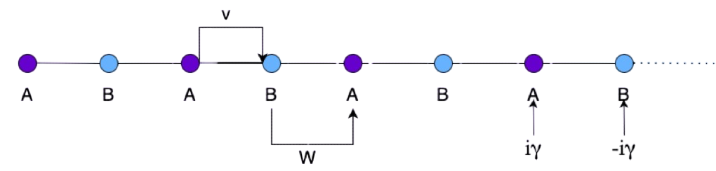
Figure 1: Schematic diagram of non-Hermitian SSH Model

This model possesses an intrinsic $\mathrm{PT}$ symmetry. The action of parity ($\mathrm{P}$) and time-reversal ($\mathrm{T}$) is defined by PhysRevLett.80.5243 ,

$$\mathrm{P}c_{A,j}\mathrm{P}=c_{B,L-j+1},\quad\mathrm{P}c_{B,j}\mathrm{P}=c_{A,L-j+1},\quad\mathrm{T}i\mathrm{T}=-i\,.$$ (2)

Using these definitions, it follows that the non-Hermitian SSH model remains invariant under the combined operation of $\mathrm{P}$ and $\mathrm{T}$, i.e.,

$$(\mathrm{PT})\,H\,(\mathrm{PT})^{\dagger}=H\,.$$

Moreover, this model preserves the total particle number,

$$Q=\sum_{j=1}^{L}\Big{(}n_{A,j}+n_{B,j}\Big{)}\,.$$ (3)

It can be shown that the non-Hermitian Hamiltonians can be used to describe the quantum dynamics of the system by continuously monitoring Hermitian Models in the no-click limit where the non-hermitian parameter is equivalent to the measurement rate 10.21468/SciPostPhys.14.5.138 . Starting with an initial state $\ket{\psi(0)}$, we can solve for $\ket{\psi(t)}$ using a deterministic equation, which is the no-click limit of the stochastic Schrödinger equation,

$$d\ket{\psi(t)}=-iHdt\ket{\psi(t)}-i\frac{dt}{2}\langle H-H^{{\dagger}}\rangle_{t}\ket{\psi(t)}\,.$$ (4)

Solving this equation, $\ket{\psi(t)}$ can be written as,

$$\ket{\psi(t)}=\frac{e^{-iHt}\ket{\psi(0)}}{||e^{-iHt}\ket{\psi(0)}||}\,.$$ (5)

Recently, it has been shown in Bhattacharya:2024hto that for certain simple non-Hermitian spin models (e.g. tight-binding model), perhaps one can study the dynamics in the Krylov space and use the spread complexity, i.e. the complexity associated with the spread of state in the Krylov space to probe the transition across the $\mathrm{PT}$ broken and non-broken phases. However, we still need more studies to establish whether the spread complexity can be used to detect this kind of $\mathrm{PT}$ phase transition or, rather, any kind of phase transition. Motivated by this, we will now study the quantum dynamics of the non-Hermitian SSH Model in the Krylov space. Interestingly, this model not only shows a $\mathrm{PT}$ transition but also gives rise to a measurement-induced entanglement phase in the $\mathrm{PT}$ broken phase where the bi-partite entanglement entropy for a subsystem, displays a transition from, volume to area law (w.r.t to the subsystem size) 10.21468/SciPostPhys.14.5.138 . One of our motivations is to investigate whether using spread complexity as well, we can detect both the $\mathrm{PT}$ transition as well as the entanglement transition. If the answer turns out to be negative, we would like to see what other relevant measure(s) in Krylov space can be used to detect this transition, particularly the entanglement one. Before studying the dynamics of this model in the Krylov space, we will briefly discuss the eigenspectrum of this model to get an insight into these transitions.

Eigenspectrum of non-Hermitian SSH model:

The eigenspectrum of the non-Hermitian Hamiltonian is generally complex. The imaginary part of the spectrum represents that the probability amplitude of the wave function will decay after a finite lifetime. The scenario is different when the system has a PT symmetry, which makes the eigenspectrum real. Since our model as mentioned in (1) is quadratic in fermionic operators, the eigenspectrum can be solved exactly. To solve this, we first perform a discrete Fourier transformation,

$$c_{\sigma,j}=\sum_{k}\frac{1}{\sqrt{L}}e^{ikj}\tilde{c}_{\sigma,k},\hskip 8.5359ptk\in\{-\pi,\pi\},\,\sigma=A,B$$ (6)

Then the Hamiltonian in (1) can be recasted in the form,

$$\begin{split}&H=\sum_{K}\begin{pmatrix}\tilde{c}_{A,k}^{{\dagger}}&&\tilde{c}_{B,k}^{{\dagger}}\end{pmatrix}\mathcal{H}_{k}\begin{pmatrix}\tilde{c}_{A,k}^{{\dagger}}\\ \tilde{c}_{B,k}^{{\dagger}}\end{pmatrix}\,,\\ &\mathcal{H}_{k}=\begin{pmatrix}i\gamma&&\eta_{k}\\ \eta_{k}^{*}&&-i\gamma\end{pmatrix}\hskip 14.22636pt\eta_{k}=-w-ve^{-ik}\,.\end{split}$$ (7)

The energy spectrum depends on the eigenvalues of the single-particle Hamiltonian $\mathcal{H}_{k}$. Diagonalizing the Hamiltonian, we can write the eigenvalues as,

$$\epsilon_{\pm,k}=\pm\sqrt{|\eta_{k}|^{2}-\gamma^{2}}=\pm\sqrt{(w^{2}+v^{2}-\gamma^{2})+2wv\cos{k}}\,.$$ (8)

Depending on the values of $w,v$ and $\gamma$, the eigenspectrum can be real or imaginary, i.e., the system will be in $\mathrm{PT}$ broken or $\mathrm{PT}$ symmetric phase. The critical value for $\mathrm{PT}$ transition is given by $u=|w-v|$ 10.21468/SciPostPhys.14.5.138 . When $(w-v)>\gamma$ and $(w-v)<-\gamma$, the system is in $\mathrm{PT}$-unbroken phase. If $-\gamma<(w-v)<\gamma$, the system will be in $\mathrm{PT}$ broken phase.

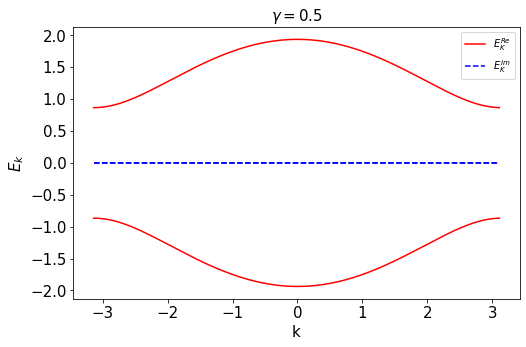
(a) $\gamma=0.5$

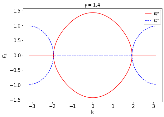
(b) $\gamma=1.4$

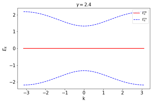
(c) $\gamma=2.4$

Figure 2: The spectrum of the non-Hermitian SSH Model for three different values of $\gamma$=0.5,1.5,2.5 (solid and dashed lines indicate the real and imaginary part of the spectrum, respectively).

Following 10.21468/SciPostPhys.14.5.138 , we will set the hopping parameters to be $w=1.5,\,v=0.5$ and vary $\gamma$ to see how the real and imaginary part of $\epsilon_{k}$ change. Then the critical value of $\gamma$ for $\mathrm{PT}$ transition is given by $\gamma=1$. As we can see from Fig. (2), for $\gamma<1$, the spectrum is purely real, and there is a finite gap at $k=\pm\pi$. At the $\mathrm{PT}$ transition point $\gamma=1$, the gap closes at the edge, and two exceptional points occur at $k=\pm\pi$. Beyond the $\mathrm{PT}$ broken region, the spectrum becomes gapless both in real and imaginary parts, and exceptional points occur at $k=\pm k_{\mathrm{EP}}(\gamma)$, whose value can be determined by 10.21468/SciPostPhys.14.5.138 ,

$$k_{\mathrm{EP}}(\gamma)=\pm 2\cos^{-1}\sqrt{\frac{\gamma^{2}-(w-v)^{2}}{4wv}}\,.$$ (9)

Putting $w=1.5$ and $v=0.5$, it can be seen that $k$ will move towards 0 when $\gamma=2$. This hints towards a second transition in the spectrum when all the eigenvalues become purely imaginary and gapped. This precisely corresponds to the entanglement transition as confirmed in 10.21468/SciPostPhys.14.5.138 by explicitly checking the late time scaling of the bi-partite entanglement entropy. Now the question is, can we capture the $\mathrm{PT}$ transition and the entanglement transition with the help of spread complexity and other relevant measures? We will try to find the answer to these questions in the next sections.

3 Spread Complexity for non-Hermitian SSH model

We now turn our attention to the Krylov Complexity PhysRevX.9.041017 . There are two notions of Krylov complexity. The first one is associated with the measures of operator growth in the Hilbert space under time evolution. But we will focus on the second one, namely the spread complexity, the complexity associated with the spread of a state in the Krylov basis under time evolution Balasubramanian:2022tpr . The key idea behind this is to find the minimal subspace accessible through the time-evolution of a given initial state $|\psi(0)\rangle\,.$ This subspace is known as ‘Krylov Space’ and is spanned by a set of orthogonal basis vectors, which can be found using the powerful algorithm known as ‘Lanczos algorithm’ viswanath1994recursion . However, the vanilla Lanczos algorithm is suitable for generating the Krylov basis only when the time evolution is governed by a hermitian Hamiltonian, i.e. when the evolution is unitary. Hamiltonian takes a tri-diagonal form when expressed in terms of the Krylov basis vectors. One needs to modify the Lanczos algorithm when the evolution is governed by a non-hermitian Hamiltonian, which is the case considered in this paper. Instead of the usual Lanczos algorithm, it is more suitable to use the ‘bi-Lanczos algorithm’ bilanczos ; Bhattacharya:2023zqt . The key idea is to generate two sets of bi-orthonormal vectors $\{|r_{j}|\rangle\}$ and $\{|l_{j}|\rangle\}$ which satisfy $\langle l_{i}|r_{j}\rangle=\delta_{ij}\,.$ Now, when one expresses the non-Hermitian Hamiltonian in terms of these bi-orthonormal basis vectors, it takes a tri-diagonal form like the Hermitian case Bhattacharya:2022gbz . We sketch the details of the bi-Lanczos algorithm in the Appendix (A) .

We will now apply this bi-Lanczos algorithm developed for our model (1). Starting with an initial state $\ket{\psi(0)}=\ket{r_{1}}=\ket{l_{1}}$ which is a product state in our case, we will generate the right and left Krylov basis $\{r_{j}\}$ and $\{l_{j}\}$. Then we can expand the time-evolved wave function $\ket{\psi(t)}$ in terms of $\{|r_{j}\rangle\}$ and $\{|l_{j}\rangle\}$ in the following way,

$$\sum_{j=1}^{\mathcal{K}}\Psi_{j}^{r}(t)\ket{r_{j}}=\ket{\psi(t)}=\sum_{j=1}^{\mathcal{K}}\Psi_{j}^{l}(t)\ket{l_{j}}$$ (10)

where $\mathcal{K}$ is the dimension of the Krylov space. The probability amplitude is defined as Bhattacharya:2022gbz ,

$$P_{j}(t)=\Big{|}\tilde{\Psi}_{j}^{r*}(t)\tilde{\Psi}_{j}^{l}(t)\Big{|}$$ (11)

where $\tilde{\Psi}_{j}^{p}$ and $\tilde{\Psi}_{j}^{q}$ are the normalized wave function in Krylov Basis. As explained in Appendix (B), the normalisation is done dynamically. This ensures the fact that $\sum_{j}^{\mathcal{K}}P_{j}(t)=1\,.$ Then following Bhattacharya:2023zqt ; Balasubramanian:2022tpr , we can define the spread complexity and spread entropy are defined as,

$$\begin{split}&\mathcal{C}(t)=\sum_{n}n\Big{|}\tilde{\Psi}_{n}^{r*}(t)\tilde{\Psi}_{n}^{l}(t)\Big{|}\,,\\ &\mathcal{S}(t)=-\sum_{n}\Big{(}|\tilde{\Psi}_{n}^{r*}(t)\tilde{\Psi}_{n}^{l}(t)|\Big{)}\ln{\Big{[}|\tilde{\Psi}_{n}^{r*}(t)\tilde{\Psi}_{n}^{l}(t)|\Big{]}}\,.\end{split}$$ (12)

Like the closed system Balasubramanian:2022tpr , it was shown in Carolan:2024wov , that the $\mathcal{C}(t)$ gets minimized when the $|\psi(t)\rangle$ is expanded in terms of the bi-orthonormal Krylov basis vectors. Also, one can define a entropic complexity Balasubramanian:2022tpr ,

$$\mathcal{C}_{S}(t)=e^{\mathcal{S}(t)}$$ (13)

where $\mathcal{S}(t)$ is defined in (12). This quantity refers to the minimum Hilbert space dimension required to store the information about the the probability distribution of Krylov basis weights Balasubramanian:2022tpr . Now, we proceed to compute these quantities for our model mentioned in (1). We will consider a lattice consisting of 40 sites, i.e., 20 unit cells. Starting with the initial state where the particle is localized on the $15^{th}$ site of the lattice, we compute the spread complexity of the evolved state for our model. Below, we summarize our results.

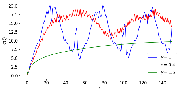
Figure 3: Time evolution of spread complexity for different values of $\gamma$ for $L=40\,.$

• It can be seen from Fig. (3), that in the $\mathrm{PT}$ symmetric phase (when $\gamma$ <1), the spread complexity oscillates with time with a large number of oscillations. At the critical point, i.e. for $\gamma=1\,,$ it oscillates, but the number of oscillations decreases. Above the transition point (i.e. $\gamma>1$), the spread complexity saturates after an initial rise. Since the eigenspectrum is real in the $\mathrm{PT}$ symmetric phase, different phases in the wave function add up to make the spread complexity oscillate. In the $\mathrm{PT}$ broken phase, the eigenspectrum is imaginary. Hence, the oscillations die down in this region and saturate at a late time. This saturation of the complexity can be attributed to the localization of wave function in the Krylov basis as reported earlier in Bhattacharya:2024hto . The spread complexity seemingly displays two types of different behaviour in these two phases. This similar to case reported for tight binding model in Bhattacharya:2024hto  . Although the result we have shown here for the non-Hermitian SSH Model with periodic boundary conditions, we have checked that this feature persists even if we use the open boundary condition.

• In Fig. (4), we have plotted the spread entropy, which was defined in (12). The spread entropy also shows a similar kind of behaviour as the spread complexity for the same initial state, and its behaviour can be explained similarly. We have also shown the behaviour of the entropic complexity (defined in (13)) in Fig. (4). Entropic complexity measures the localization strength. The saturation of entropic complexity also reflects the localization of wave function in the $\mathrm{PT}$ broken phase. This supports our earlier observation.

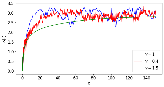
(a) $\textrm{Spread Entropy}(\mathcal{S}(t))$

(b) $\textrm{Entropic complexity}(\mathcal{C}_{S}(t))$

Figure 4: Time evolution of spread entropy, and entropic complexity different values of $\gamma$ for $L=40\,.$

So far, we have focused on the behaviour of spread complexity and associated quantities across the $\mathrm{PT}$ transition point. As mentioned earlier, our model also displays a measurement-induced phase transition at $\gamma=2\,$. We will now focus on the spread complexity and entropy across this transition point and analyse their behaviour to see whether we can detect such transition through these quantities. We make the following observations.

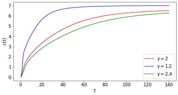
(a) Spread Complexity

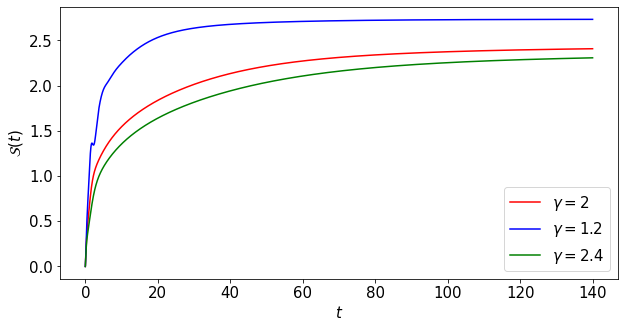
(b) Spread Entropy

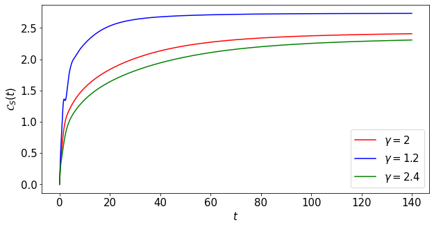
(c) Entropic complexity

Figure 5: Time evolution of spread complexity, spread entropy and entropic complexity beyond the $\mathrm{PT}$ symmetric region .

• In Fig. (5), we have shown that spread complexity saturates above the $\mathrm{PT}$ symmetric region. From Fig. (5), it can be seen that as the value of the non-hermiticity parameter ($\gamma$) increases, the saturation value of the spread complexity, spread entropy, and entropic complexity decreases and the saturation timescale increases. To understand the reason behind the lower saturation value of $\mathcal{C}(t)$ for higher values of $\gamma$, one can investigate the Krylov inverse participation ratio (KIPR). We checked that the saturation value of KIPR increases with increasing value of $\gamma$. A higher value of KIPR indicates stronger localization. If the state is more localized, the spread of the state will be less. This is the reason behind the lower saturation value of the spread complexity with increasing $\gamma$ irrespective of the measurement-induced transition point. This is consistent with what has been reported in Bhattacharya:2024hto for the tight-binding model.

• To clarify things, we plot the saturation timescale of spread complexity and entropy as a function of $\gamma$ in the PT broken phase, especially around the entanglement transition point in Fig. (6). We find that the saturation time scale increases with the increase of non-hermiticity parameter $\gamma$, but it is insensitive to entanglement transition.

  

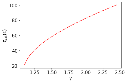
  (a) Saturation time scale of spread complexity

  

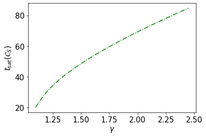
  (b) Saturation time scale of entropic complexity

  Figure 6: Saturation timescale of the spread complexity and entropic complexity as a function of measurement rate $\gamma\,.$

• Keeping in mind that the measurement-induced transition can be detected by looking at the scaling of entanglement entropy with respect to (sub) system size PhysRevB.103.224210 ; 10.21468/SciPostPhysCore.6.3.051 , we investigate the scaling of the spread complexity with respect to the system size ($L$) around this transition point (i.e around $\gamma=2$) .

  

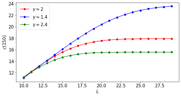
  Figure 7: Late-time spread complexity for different system size $L\,.$

  As can be seen from Fig. (7), the spread complexity initially increases following a saturation for a larger system size ($L$). The initial increase in spread complexity decreases with $\gamma$, and the saturation value decreases with measurement rate $\gamma$. Also, from Fig. (7), it seems that there is a change in the scaling behaviour of the spread complexity from linear to sub-linear as we increase the value of the $\gamma\,$ To make this observation concrete, we have checked the scaling of spread complexity: $\mathcal{C}\propto L^{\alpha}$ and found that $\alpha$ smoothly decreases across the $\gamma=2$ without showing any jump. The scaling factor($\alpha(\gamma)$) is unable to detect the entanglement transition point ($\gamma=2$). The reason behind this failure to detect entanglement transition could be the absence of information of any subsystem. Unlike the entanglement entropy for a subsystem, we are looking at the complexity of the state for the entire system. Keeping this in mind; in the next section, we will extend our investigation of the spread complexity for a subsystem and try to see whether it can capture this measurement-induce transition.

Spread Complexity for a subsystem in Krylov Space:

We now turn our attention to the complexity of a subsystem in the Krylov space. Starting with an initially localized state in real space, we applied the bi-Lanczos algorithm for our Hamiltonian model (1). We expand the initial state $|\psi(0)\rangle$ in terms of Krylov basis vectors and evolve the state using the procedure explained in Appendix (B). After that, we construct the density matrix $\rho(t)$ as mentioned in (49) and expand in terms of Krylov basis vectors. From this, we calculate the reduced density matrix $\rho_{\textrm{A}}=\Tr_{\textrm{B}}\rho$ by taking the reduced trace over a subspace in Krylov space. Now, we like to compute the spread complexity for this $\rho_{\textrm{A}}\,.$ Note that $\rho_{\textrm{A}}$ corresponds to a mixed state. Then, taking a cue from the measures for entanglement for a mixed state such as “Entanglement of Purification”($\mathrm{EoP}$) and a similar measure for circuit complexity such as “Complexity of Purification” ($\mathrm{CoP}$) Nguyen:2017yqw ; PhysRevLett.122.201601 ; PhysRevResearch.3.013248 ; Bhattacharyya:2020iic ; Bhattacharyya:2021fii ; Bhattacharya:2022wlp ; Bhattacharyya:2022rhm we use the Choi–Jamiołkowski isomorphism to purify this $\hat{\rho}_{A}$ to get a pure state in the doubled Hilbert space. An operator $\hat{O}$ can be expanded in terms of a orthonormal basis $|i\rangle$ in the following way:

$$\hat{O}=\sum_{i\,,j}O_{ij}|i\rangle\langle j|\,.$$

Then following PhysRevA.87.022310 one can associate a state with this operator via channel-state duality/Choi–Jamiołkowski isomorphism,

$$\hat{O}=\sum_{i\,,j}O_{ij}|i\rangle\langle j|\leftrightarrow|\hat{O}\rangle=\frac{1}{\sqrt{\Tr(O^{\dagger}O)}}\sum_{i,j}\,O_{ij}|i\rangle\otimes|j\rangle\,.$$ (14)

This idea can be used to purify the reduced density matrix $\hat{\rho}_{A}$. We have expanded $\hat{\rho}_{A}$ in terms of its eigenbasis (which forms an orthonormal basis).

$$\hat{\rho}_{A}=\frac{1}{\sqrt{\sum_{j}\lambda^{2}_{j}}}\sum_{i}\lambda_{i}|\lambda_{i}\rangle\langle\lambda_{i}|$$

where $\lambda_{i}s$ denote the eigenvalues and $|\lambda_{i}\rangle$ are the eigenvectors. After that, using the channel-state duality we get,

$$|\hat{\rho}_{A}\rangle=\frac{1}{\sqrt{\sum_{j}\lambda^{2}_{j}}}\sum_{i}\lambda_{i}|\lambda_{i}\rangle\otimes|\lambda_{i}\rangle\,.$$

Then one can use the same procedure outlined at the beginning of this section to compute the spread complexity of purification (kCoP) using the bi-Lanczos coefficients generated earlier  .

• Next, we analyze the scaling of late time kCoP with sub-system size. It takes the following form

  $$\textrm{kCoP}\propto\ell^{\alpha(\gamma)}\,.$$

  

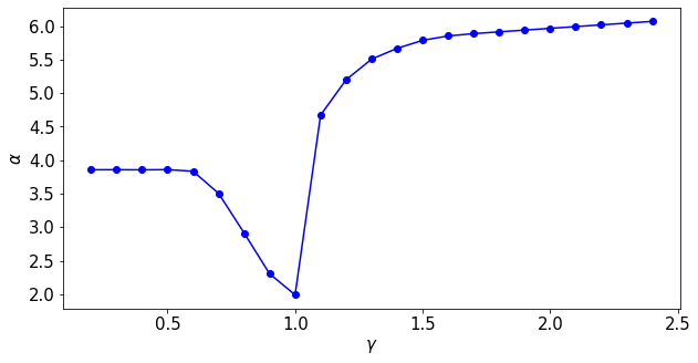
  Figure 8: Behaviour of the scale factor associated with the power law scaling of late time kCoP with $\gamma\,.$

  Fig. (8) shows the variation of $\alpha$ with respect to the measurement rate $\gamma\,.$ It shows a dip at $\gamma=1$, which is the $\mathrm{PT}$ transition point, then sharply increases before reaching a plateau. So we can see that, using the late time scaling of the kCoP, we can detect the $\mathrm{PT}$ transition point quite effectively, although it fails to detect the measurement-induce transition point ($\gamma=2$).

• Recently, it has been shown in PhysRevB.109.224304 that the time-averaged Krylov complexity can act as an order parameter for phase transitions for a certain model (e.g., the Lipkin-Meshkov-Glick model). Motivated by this idea, we now investigate the time averaged kCoP to check whether it can be an order parameter for our case. The time average kCoP is defined as,

  $$\bar{C}_{K}=\frac{1}{T-\textrm{tref}}\int_{\textrm{tref}}^{T}C_{K}(t)\,dt\,.$$ (15)

  In Fig. (9), we plot $\bar{C}_{K}$ as a function of measurement rate $\gamma\,.$

  

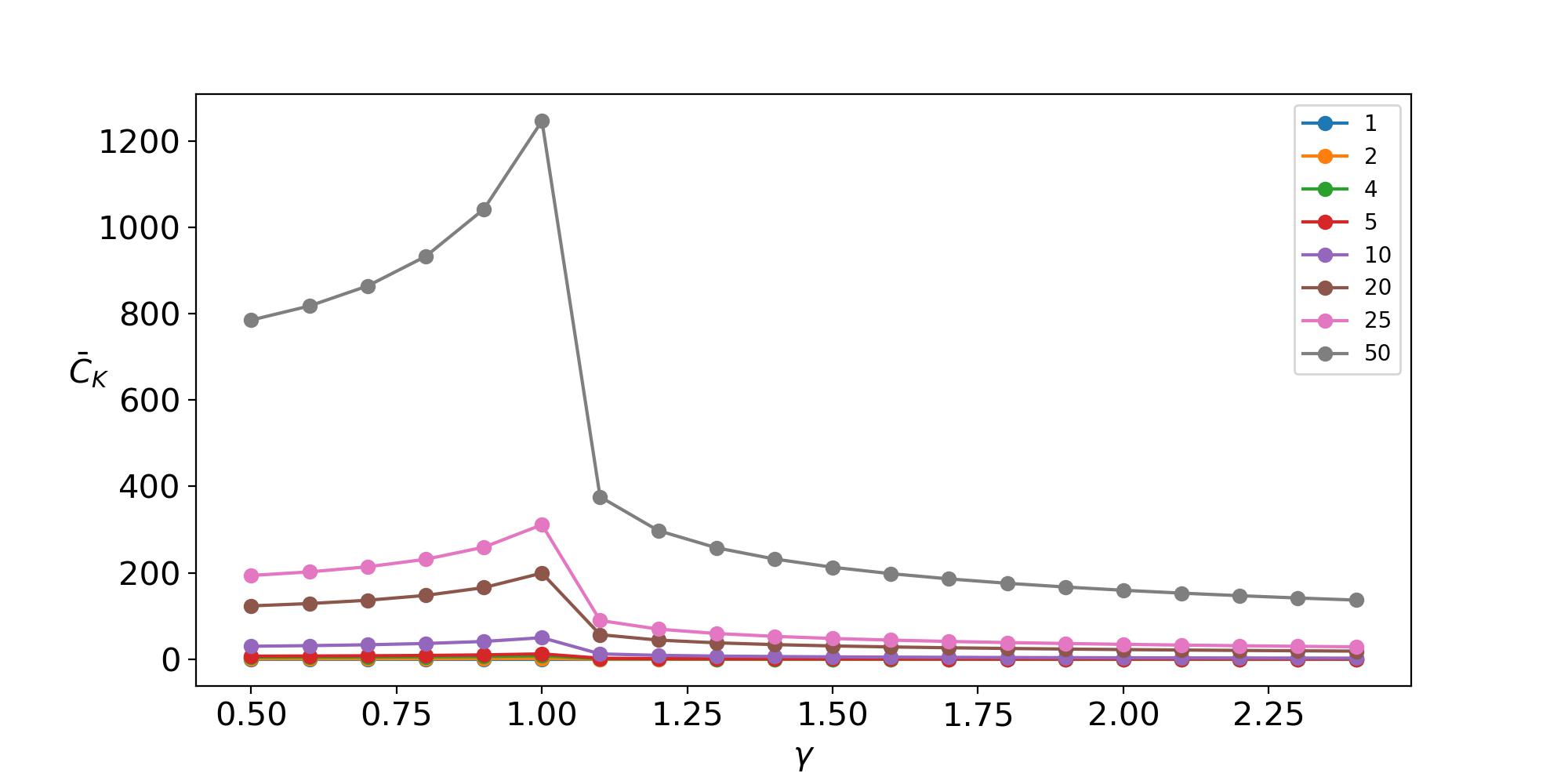
  Figure 9: $\bar{C}_{K}$ vs $\gamma$ for different sub-system size for the a system of size $L=100\,.$

  For small sub-systems, PT transition can not be detected through $\bar{C}_{K}$. As the subsystem size increases, we can see a sharp transition around the PT transition point, i.e., $\gamma=1$, and it starts to become independent of $\gamma$ for higher values of $\gamma$ irrespective of the measurement-induced transition point. We also explore the scaling of $\bar{C}_{K}\propto$ $\ell^{\alpha}$ and plot $\alpha$ as a function of $\gamma$ in Fig. (11). It can be seen that it changes sharply near $\gamma=1$, which is the PT transition point.

  

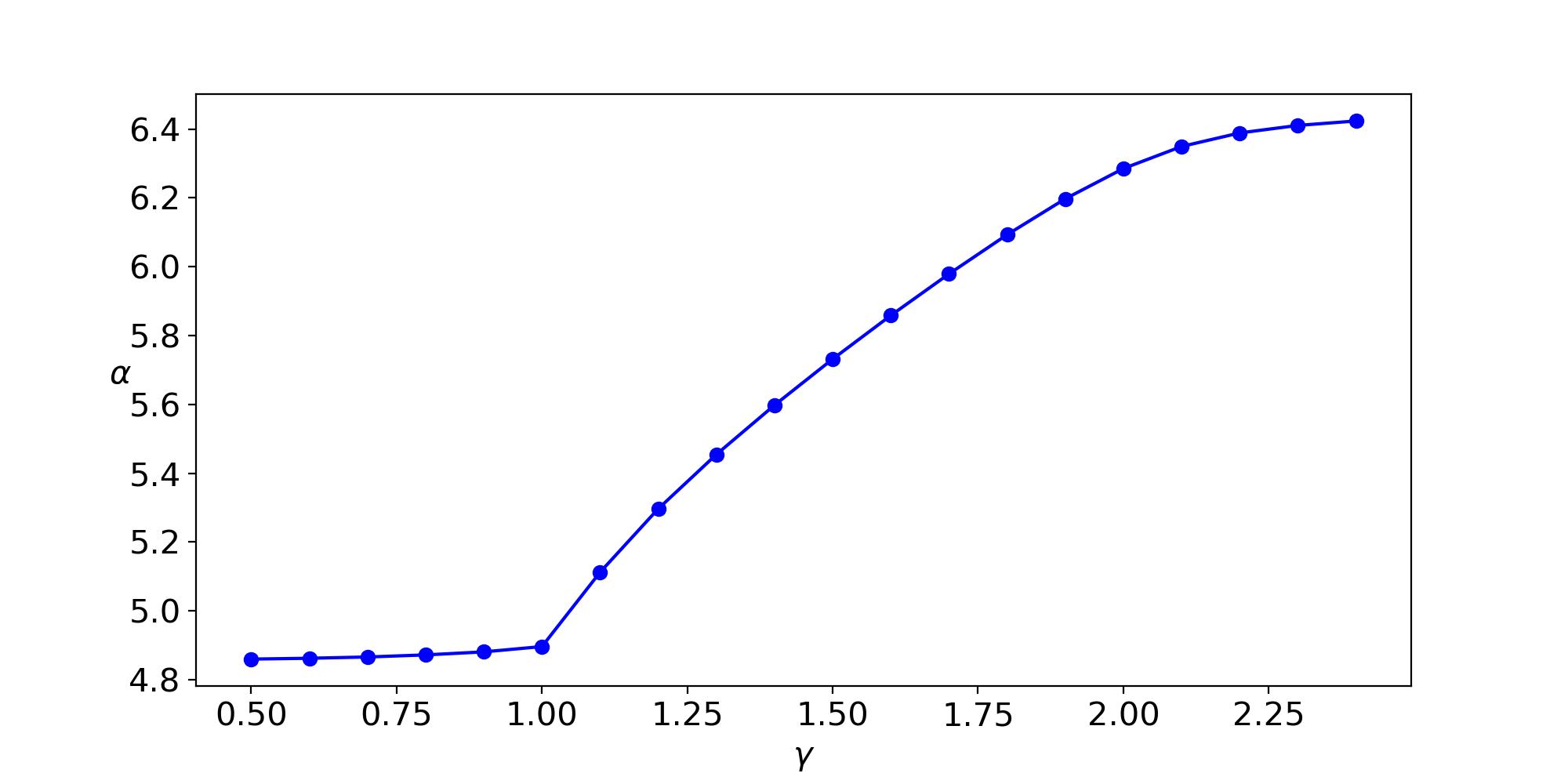
  Figure 10: Scaling of $\bar{C}_{K}$ as a function of $\gamma\,.$

So we conclude that the scaling of the late time value of the $\mathrm{kCoP}$ (with respect to subsystem size) can serve as a good indicator (in fact, better than the spread complexity evaluated earlier for the whole system) for the $\mathrm{PT}$ transition, as its behaviour changes sharply across the transition point, but still $\mathrm{kCoP}$ cannot probe the measurement-induced transition point. It is still insensitive to the correlation between the subsystem and its complement in real space, unlike the entanglement entropy.

In the next section, we focus on another quantity, namely and Quantum Fisher Information, which, when evaluated in the Krylov space, possesses a structural similarity to the Krylov complexity Shi:2024bpu ; PhysRevLett.133.110201 . Motivated by this fact, we will explore this quantity to see whether it can detect the entanglement transition.

4 Quantum Fisher information in Krylov space

Quantum Fisher information (QFI) is a central object in quantum measurement and quantum metrology. The classical Fisher information describes how rapidly a probability distribution changes with respect to some parameters. Similarly, QFI describes how fast a quantum state changes with respect to some parameter. QFI has been used to detect quantum phase transition Wang_2014 ; PhysRevB.100.184417 as well as the scaling of time-averaged QFI has been used as a diagnostics of quantum chaos Shi:2024bpu . Recently, it has been shown that the time-averaged QFI can be used to detect the measurement-induced phase transition for models (collective spin systems) Poggi:2023mll . Furthermore, from the analysis of Shi:2024bpu ; PhysRevLett.133.110201 , that QFI possess a structural similarity with the Krylov complexity when decomposed in terms of Krylov basis. We will elaborate more on this shortly. Motivated by these, we investigate the time-averaged QFI in Krylov space for our model to possibly detect the measurement-induced entanglement transition in the PT broken region.

The QFI for a pure state $|\psi(t)\rangle$ can be defined for an operator $\hat{O}$ in the following way Pezze:2016nxl ; 2014JPhA…47P4006T ; Chu:2023mzh ; Shi:2024bpu ; PhysRevLett.133.110201 ,

$$F_{Q}[\ket{\psi(t)},\hat{O}]=4(\Delta\hat{O}(t))^{2})=4(\bra{\psi(t)}\hat{O}^{2}\ket{\psi(t)}-\bra{\psi(t)}\hat{O}\ket{\psi(t)}^{2}).$$ (16)

where $\ket{\psi(t)}$ is given by equation (5).
The time-averaged QFI can then be defined same as in (15),

$$\bar{F}[\hat{O}]=\frac{1}{T-t_{ref}}\int_{t_{ref}}^{T}F_{Q}[\ket{\psi(t)},\hat{O}]\,dt\,.$$ (17)

For our case, we will focus on studying this quantity in Krylov space. We do it in two ways: firstly, by expanding the state in terms of the Krylov basis and, secondly, by expanding the operator in the Krylov space.

Krylov expansion of state

The time-evolved state $|\psi(t)\rangle$ can be expanded in Krylov basis as,

$$\ket{\psi(t)}=\sum_{j=1}^{\mathcal{K}}\Psi_{j}^{r}(t)\ket{r_{j}}=\sum_{j=1}^{\mathcal{K}}\Psi_{j}^{l}(t)\ket{l_{j}}\,.$$ (18)

The expectation values of the operators can be expanded in terms of the Krylov basis as

$$\langle{O^{k}(t)}\rangle=\sum_{j,j^{\prime}=1}^{\mathcal{K}}{\Psi_{j}^{l*}(t)\Psi_{j^{\prime}}^{r}(t)\bra{l_{j}}O^{k}\ket{r_{j}^{\prime}}}\,.$$ (19)

For our non-hermitian SSH model the measurement operators are $\hat{n}_{A}$ for sub-lattice $A$ and $I-\hat{n}_{B}$ for sub-lattice $B$. We have computed time-averaged QFI using (17) for the measurement operators $\hat{n}_{A}$ and $I-\hat{n}_{B}$ for different system sizes and for different measurement rate $\gamma\,.$

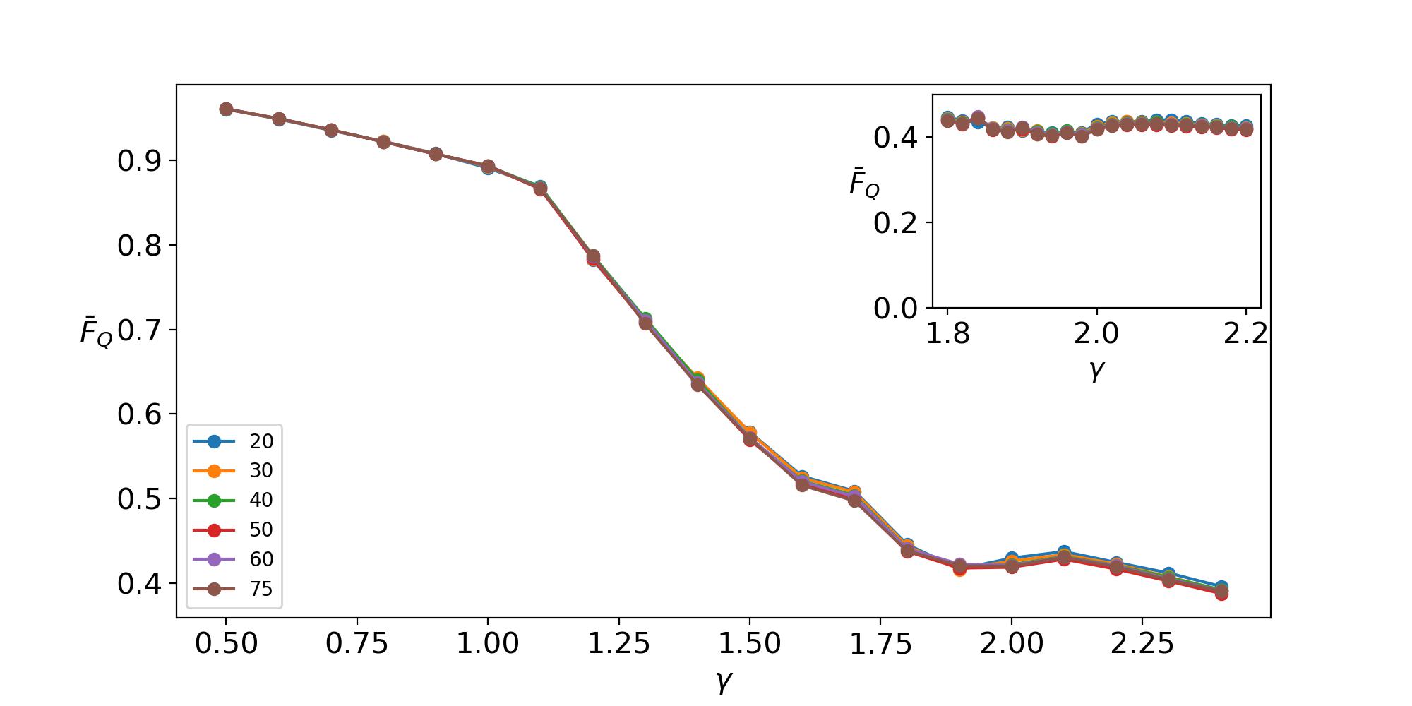
Figure 11: Time-averaged QFI as a function of $\gamma$ for different system size. In the inset, we have shown the behaviour of QFI around the measurement-induced transition point, i.e. $\gamma=2\,.$

Now we make the following observations:

• From Fig. (11), it is evident that the nature of the $\bar{F}_{Q}$ is insensitive to the system size .

• Secondly, it can be seen from Fig. (11), that $\bar{F}_{Q}$ decreases with increasing value of $\gamma$. There is a change of its slope at $\gamma=1$ (PT transition point), and it almost becomes independent of $\gamma$ around $\gamma=2$. We have shown the behaviour of $\bar{F}_{Q}$ near $\gamma=2$ in the inset of Fig. (11). So we can conclude that the time-averaged QFI can detect the measurement-induced transition in our model besides serving as a probe for PT transition .

Krylov expansion of the operator

Next, we will use the Heisenberg picture to write the QFI for a pure state in the following way,

$$F_{Q}(\rho(t),\hat{O})=4\Bigg{(}\frac{1}{N^{2}}\bra{\psi(0)}\hat{O}^{2}(t)\ket{\psi(0)}-\frac{1}{N^{4}}\bra{\psi(0)}\hat{O}(t)\ket{\psi(0)}^{2}\Bigg{)}$$ (20)

where $\hat{O}(t)$ (for a generic non-Hermitian $H$) can be expressed as,

$$\hat{O}(t)=e^{iH^{{\dagger}}t}\hat{O}(0)e^{-iHt}\,,\quad N=||e^{-iHt}\ket{\psi(0)}||\,.$$ (21)

As mentioned previously, $\hat{O}(0)$ for our case will be the measurement operator $\hat{n}_{A}$ and $I-\hat{n}_{B}$ and the Hamiltonian is given by (1). Since our Hamiltonian is non-Hermitian, we will use the bi-Lanczos method (extending it for the operators) to find the left and right Lanczos coefficients and the left and right Krylov basis. The details are given in Appendix (A). Then we can expand the operator $\hat{O}(t)$ as,

$$\begin{split}\hat{O}(t)=\sum_{m}i^{m}\phi_{m}^{R}(t)\hat{O}_{r_{m}}\,,\\ =\sum_{n}i^{n}\phi_{n}^{L}(t)\hat{O}_{l_{n}}\end{split}$$ (22)

where $\phi_{m}^{R}(t)$ and $\phi_{m}^{L}(t)$ are the operator wave function and $\hat{O}_{r_{m}},\hat{O}_{l_{n}}$ are the right and left Krylov basis as defined in (41).

For our case using the expansion (22) we can re-write the expression for QFI as ,

$$\begin{split}F_{Q}(\rho(t),\hat{O})=4\Bigg{(}\sum_{m,n}&\frac{i^{m+n}}{N^{2}}\Big{\{}(-1)^{m}\phi_{m}^{R*}(t)\phi_{n}^{L}(t)\langle{O_{r_{m}}^{{\dagger}}O_{l_{n}}\rangle}+(-1)^{n}\phi_{m}^{R}(t)\phi_{n}^{L*}(t)\langle{O_{r_{m}}O_{l_{n}}^{{\dagger}}\rangle}\Big{\}}-\\ &\frac{i^{m+n}}{N^{4}}\Big{\{}\phi_{m}^{R}(t)\phi_{n}^{L}(t)\langle{O_{r_{m}}}\rangle\langle{O_{l_{n}}}\rangle\Big{\}}\Bigg{)}\,.\end{split}$$ (23)

Note that, for a unitary evolution, the normalization factor, $N=1$ and

$$\begin{split}\phi_{m}^{R*}(t)=\phi_{m}^{R}(t)=\phi_{m}(t)\,,\quad\phi_{n}^{L*}(t)=\phi_{n}^{L}(t)=\phi_{n}(t)\,,\quad O_{r_{m}}^{{\dagger}}=O_{m},O_{l_{n}}=O_{n}\,.\end{split}$$ (24)

Then the expression for the QFI in Krylov space as mentioned (23) reduces to,

$$F_{Q}(\rho(t),\hat{O})=4\sum_{m,n}i^{m+n}\phi_{m}(t)\phi_{n}(t)\underbrace{\Big{(}((-1)^{m}+(-1)^{n})\langle O_{m}O_{n}\rangle-\langle{O_{m}}\rangle\langle{O_{n}}\rangle\Big{)}}_{f_{(m,n)}}\,.$$ (25)

This is structurally equivalent to Krylov complexity. In PhysRevLett.133.110201 , authors came up with a variant of the QFI using (25) in the correlation landscape to qualitatively capture dynamical behaviour, which is proportional to the Krylov complexity. In general, one can think of (25) as a generalization of the complexity functional encapsulating the information of the underlying correlation. For non-unitray evolution, this further generalizes to (23) as mentioned earlier.

Now motivated by these facts, following our previous analysis regarding Krylov complexity, we now calculate the time-averaged QFI as defined in (17) in Krylov space for different system sizes for various values of measurement rate $\gamma$.

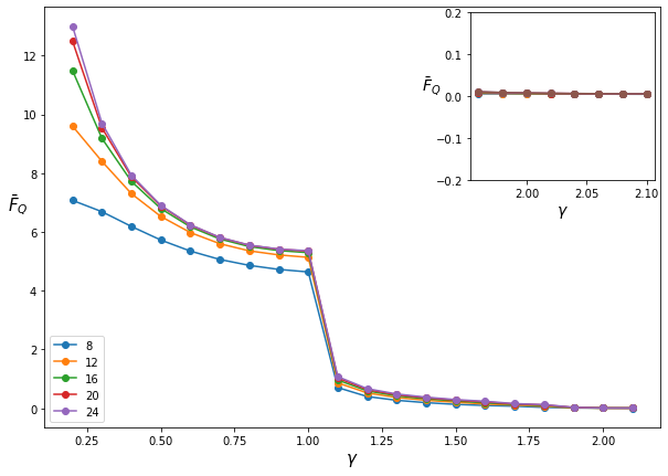
Figure 12: Time-averaged QFI as a function of $\gamma$ for different system size. In the inset, we have shown the behaviour of QFI around the measurement-induced transition point, i.e. $\gamma=2\,.$

Now we summarize our observations:

• It is evident from the Fig. (12), that the behaviour time-averaged QFI ($\bar{F}_{Q}$) is independent of the system size (except for small values of $\gamma$). Initially it starts from a higher values and it slope changes sharpely across the PT transition point i.e $\gamma=1\,.$

• Furthermore, it saturates and becomes vanishing small across the measurement induced transition point i.e $\gamma=2\,.$ This has been highlighted in the inset of the Fig. (12) .

Finally, we can conclude that the QFI (time-averaged), which is of similar structure to that of the Krylov complexity when expanded in terms of Krylov basis but captures the information of the underlying correlation (which is missing from the Krylov complexity functional), can capture the measurement induced transition along with being a probe for PT transition.

5 Discussion and outlook

Motivated by the recent studies of the dynamics of quantum many-body systems in Krylov space and the complexity associated with the spread of state/operator in the Krylov space PhysRevX.9.041017 ; Nandy:2024htc , we have initiated a study of the dynamics of a monitored SSH model (in no-click limit) in Krylov space. This model not only shows a $\mathrm{PT}$ transition but also gives rise to a measurement-induced entanglement phase in the $\mathrm{PT}$ broken phase 10.21468/SciPostPhys.14.5.138 . We first observed that, for this non-hermitian $\mathrm{SSH}$ chain, measures like spread complexity, spread entropy, and entropic complexity show oscillatory behaviour below the PT symmetric point. On the other hand, they show a linear behaviour at early times followed by a late time saturation after the PT symmetric point. It persists even across the measurement-induced transition point i.e. across $\gamma=2\,.$ This is consistent with the earlier observations in Bhattacharya:2024hto for a tight-binding chain with non-hermitian potential at the two edges . Next, we have found that in the $\mathrm{PT}$ broken region, the saturation value of these measures decreases as the value of $\gamma$ increases. With the increase in the value of $\gamma$ , the wave function becomes more localized, and due to this reason, the suppression of spread complexity and the other associated measures happens. We also found that the saturation timescale ($t_{\mathrm{sat}}$) is an increasing function of $\gamma\,.$ Furthermore, keeping in mind the entanglement transition, we have investigated the scaling of the spread complexity with system size at a late time, and it takes the following form: $C_{k}\propto L^{\alpha},$ where the scaling exponent $\alpha$ smoothly decreases with the increasing value of $\gamma$ irrespective of the entanglement transition. Overall, although the late time behaviour of the spread complexity (for the full system) shows different behaviour across the PT transition, it fails to capture the entanglement transition.

Next, we extended the notion of the spread complexity for a subsystem in the Krylov space by utilizing purification techniques. We found that scaling of the Krylov complexity of purification (kCoP) with the sub-system size. The scaling exponent displays a sharp minima at the PT transition point i.e. $\gamma=1$, but keeps increasing beyond that irrespective of entanglement transition. Also, we compute the time-averaged kCoP and find that it has a dip near PT transition point. This behaviour is more prominent for larger sub-system sizes. Overall, we can see that the kCoP displays a sharp transition across the PT transition point and can serve as a good indicator (better than the spread complexity for the full system) of probing such transition but like the full system complexity it again fails to capture the entanglement transition.

Unlike the entanglement entropy, the spread complexity functional is insensitive to the correlation present in the underlying system. But in recent times, in Shi:2024bpu ; PhysRevLett.133.110201 , it has been shown that the Quantum Fisher Information (QFI), when evaluated in the Krylov space, possesses structural similarity to the Krylov complexity but contains the information about the correlation landscape of the underlying system. In fact, we treat the expression of QFI in the Krylov space as a generalized complexity functional and explore this quantity to see whether it can detect the entanglement transition. We calculate the QFI for the measurement operator by expanding either the state or the operator in the Krylov space. From both these two cases, we have found that QFI (in Krylov space) decreases with increasing value of $\gamma$, which changes the slope around $\gamma=1$ and almost becomes independent of $\gamma$ around $\gamma=2$. From this behaviour of QFI, we can conclude that QFI can detect the measurement-induced transition along with detecting the usual PT transition.

Finally, we conclude by pointing out some future directions. First of all, it will be interesting to generalize our study beyond the no-click limit. For that, the time evolution will be governed by the full stochastic Schrödinger equation. Then, one can perhaps find the Lanczos coefficients using the moment method from the overlap of the final and initial state following viswanath1994recursion ; Balasubramanian:2022tpr ; Caputa:2024vrn . Furthermore, it will be interesting to generalize the computation of spread complexity for a subsystem in the position space for a time-evolved state. This will perhaps help us to make a more direct comparison with the result of entanglement entropy. Again, one will have to use the idea of purification. Last but not least, the idea of using QFI in Krylov space to detect measurement-induced transition is something which remains to be investigated for various other interesting monitored models, which we hope to do in near future.

Appendix A Bi-Lanczos algorithm overview

Krylov operator/state complexity is usually defined by well-known Lanczos coefficients PhysRevX.9.041017 ; viswanath1994recursion  . However, this is valid only for the case when the time evolution is unitary, i.e. the Hamiltonian is hermitian. Modifications in the Lanczos algorithm are required to define Krylov operator/state complexity for non-unitary evolution. Arnoldi’s recursive technique has been applied to extend the Lanczos algorithm for such non-hermitian cases Bhattacharya:2022gbz ; Bhattacharyya:2023grv . However, this technique converts the Hamiltonian into an upper-Hessenberg matrix instead of a tridiagonal form. The bi-Lanczos algorithm can deal with this problem, which gives us a tridiagonal form of a non-hermitian matrix Bhattacharya:2023zqt ; Bhattacharya:2023yec . For our studies presented in this paper, we will be required to expand both a state and an operator in terms of the basis generated by the bi-Lanczos algorithm. We discuss them separately below.

For states:

The non-Hermitian matrix acts differently on the ket vector and bra vector. Therefore, instead of defining a single initial state, we introduce two initial vectors/states $\ket{r}$ and $\bra{l}=\ket{r}^{{\dagger}}$. Using the two-sided Gram-Schmidt procedure for $\ket{r_{1}}$ and $\bra{l_{1}}$,we get Krylov subspaces $\{A\ket{r_{1}},A^{2}\ket{r_{1}},\ldots\}$ and $\{\bra{l_{1}}A,\bra{l_{1}}A^{2},\ldots\}$ spanned by $\{\ket{r_{1}}\}$ and $\{\bra{l_{1}}\}$, respectively.
Using the two initial vectors, further vectors are constructed (following bi-orthogonality with each iteration) using the following recursion relations:

$$c_{j+1}\ket{r_{j+1}}=A\ket{r_{j}}-a_{j}\ket{r_{j}}-b_{j}\ket{r_{j-1}}$$

$$b^{*}_{j+1}\ket{l_{j+1}}=A^{\dagger}\ket{l_{j+1}}-a^{*}_{j}\ket{l_{j}}-c^{*}_{j}\ket{l_{j-1}}.$$

The non-hermitian matrix $A$ takes the following tri-diagonal form in this new basis:

$$\begin{bmatrix}a_{1}&b_{2}&0&\ldots&0\\ c_{2}&a_{2}&b_{3}&&0\\ 0&\ddots&\ddots&\ddots&\\ \vdots&&c_{j-1}&a_{j-1}&b_{j}\\ 0&\ldots&0&c_{j}&a_{j}\\ \end{bmatrix}.$$

Here, we present a step-by-step bi-Lanczos algorithm for a non-hermitian matrix A, which provides us with all the coefficients required to define the Krylov complexity.

For j=1:

(a) Choose the initial set of vectors $\ket{r_{1}}$ and $\ket{l_{1}}$ with orthonormality condition $\innerproduct{l_{1}}{r_{1}}=1$ and initial lanczos coefficients as $a_{1}=\bra{l_{1}}A\ket{r_{1}}$, $b_{1}=0$ and $c_{1}=0$.

For j>1:

(a) Act matrix A on $\ket{r_{j}}$ and $A^{{\dagger}}$ on $\ket{l_{j}}$. We obtain the following new vectors:

$$\ket{\alpha_{j}^{\prime}}=A\ket{r_{j}},\ket{\beta_{j}^{\prime}}=A^{\dagger}\ket{l_{j}}.$$ (26)

(b) Construct orthogonal basis vectors by subtracting the contribution from two previous basis vectors $\ket{r_{j}}$, $\ket{r_{j-1}}$ and similarly for $\ket{l_{j}}$ and $\ket{l_{j-1}}$.
The new orthogonal vectors are:

$$\ket{\alpha_{j}}=\ket{\alpha_{j}^{\prime}}-a_{j}\ket{r_{j}}-b_{j}\ket{r_{j-1}},\ket{\beta_{j}}=\ket{\beta_{j}^{\prime}}-a^{*}_{j}\ket{l_{j}}-c^{*}_{j}\ket{l_{j-1}}.$$ (27)

(c) The value of the next Lanczos coefficients $c_{j+1}$ and $b_{j+1}$ is given by:

$$c_{j+1}=\sqrt{\absolutevalue{\omega_{j}}},b_{j+1}=\frac{\omega_{j}}{c_{j+1}}$$ (28)

where, $\omega_{j}$ is obtained by taking inner product of vectors $\ket{\alpha_{j}}$ and $\ket{\beta_{j}}$ : $\omega_{j}=\langle{\alpha_{j}}|{\beta_{j}}\rangle$.

(d) Since $\ket{\alpha_{j}}$ and $\ket{\beta_{j}}$ are not normalised, construct normalized basis vectors $\ket{\alpha_{j+1}}$ and $\ket{\beta_{j+1}}$ of Krylov basis:

$$\ket{r_{j+1}}=\frac{\ket{\alpha_{j}}}{c_{j+1}},\ket{l_{j+1}}=\frac{\ket{\beta_{j}}}{b^{*}_{j+1}}\,.$$ (29)

(e) For successive iterations, subtracting the contribution from only the previous two basis vectors can lead to significant numerical error. It can be resolved by the Gram-Schmidt orthogonalization technique, which subtracts the contribution of all the previous vectors.

For the bi-Lanczos algorithm, bi-orthogonalization is used:

$$\ket{r_{j}}=\ket{r_{j}}-\sum_{m=1}^{j-1}\langle{l_{m}}|{r_{m}}\rangle\ket{r_{m}}\,,$$ (30)

$$\ket{l_{j}}=\ket{l_{j}}-\sum_{m=1}^{j-1}\langle{r_{m}}|{l_{m}}\rangle\ket{l_{j}}\,.$$ (31)

(f) Finally, the diagonal element of the tridiagonal matrix $a_{j+1}$ is obtained by:

$$a_{j+1}=\bra{l_{j+1}}A\ket{r_{j+1}}\,.$$ (32)

For operators:

The operator equation for non-Hermitian evolution is given by,

$$\hat{O}(t)=e^{iH^{{\dagger}}t}\hat{O}(0)e^{-iHt}\,.$$ (33)

The equation of motion satisfied by the operator $\hat{O}(t)$,

$$\partial_{t}\hat{O}(t)=H^{{\dagger}}\hat{O}(t)-\hat{O}(t)H\,.$$ (34)

Then, the Liouvillian super-operator can be defined by,

$$\mathcal{L}\hat{O}(t)=H^{{\dagger}}\hat{O}(t)-\hat{O}(t)H\,.$$ (35)

Now, we will discuss the bi-Lanczos algorithm step by step.

For j=1:

(a) Choose the initial set of operators $\hat{O}_{r_{1}}$ and $\hat{O}_{l_{1}}$ with orthonormality condition
$\langle\hat{O}_{l_{1}}|\hat{O}_{r_{1}}\rangle=1$ where the inner product of two operators is defined as,

$$\langle{\hat{O}_{1}}|{\hat{O}_{2}}\rangle=\frac{1}{\sqrt{D}}\Tr(\hat{O}_{1}^{{\dagger}}\hat{O}_{2})$$ (36)

and the initial Lanczos coefficients are $b^{1}_{\textrm{up}}=0$ and $b^{1}_{\textrm{down}}=0\,.$

For j>1:

(a) Acting with the Liouvillain super-operator on $\hat{O}_{r_{j}}$ and $\hat{O}_{l_{j}}$ we can obtain the new operators.

$$\hat{O}_{\alpha_{j}^{\prime}}=H^{{\dagger}}\hat{O}_{r_{j}}-\hat{O}_{r_{j}}H,\hskip 5.69046pt\hat{O}_{\beta_{j}^{\prime}}=H^{{\dagger}}\hat{O}_{l_{j}}-\hat{O}_{l_{j}}H.$$ (37)

(b) Construct orthogonal basis vectors by subtracting the contribution from two previous basis operators $\hat{O}_{r_{j}}$, $\hat{O}_{r_{j-1}}$ and similarly for $\hat{O}_{l_{j}}$ and $\hat{O}_{l_{j-1}}$. The new orthogonal vectors are:

$$\hat{O}_{\alpha_{j}}=\hat{O}_{\alpha_{j}^{\prime}}-b^{\textrm{up}}_{j}\hat{O}_{r_{j-1}}\,,\quad\hat{O}_{\beta_{j}}=\hat{O}_{\beta_{j}^{\prime}}-(b^{\textrm{down}}_{j})^{*}\,\hat{O}_{l_{j-1}}\,.$$ (38)

(c) The value of the next Lanczos coefficients $b^{\textrm{up}}_{j+1}$ and $b^{\textrm{down}}_{j+1}$ is given by:

$$b^{\textrm{down}}_{j+1}=\sqrt{\absolutevalue{\omega_{j}}},b^{\textrm{up}}_{j+1}=\frac{\omega_{j}}{b^{\textrm{down}}_{j+1}}\,.$$ (39)

where $\omega_{j}=\langle{\hat{O}_{\alpha_{j}}}|\hat{O}_{\beta_{j}}\rangle\,.$

(d) We can then construct the normalized basis vectors $\hat{O}_{\alpha_{j+1}}$ and $\hat{O}_{\beta_{j+1}}$ :

$$\hat{O}_{r_{j+1}}=\frac{\hat{O}_{\alpha_{j}}}{b^{\textrm{down}}_{j+1}},\hat{O}_{l_{j+1}}=\frac{\hat{O}_{\beta_{j}}}{(b^{\textrm{up}}_{j+1})^{*}}\,.$$ (40)

(e) For successive iterations, subtracting the contribution from only the previous two basis vectors can lead to significant numerical error. It can be resolved by the Gram-Schmidt orthogonalization technique, which subtracts the contribution of all the previous vectors.

$$\begin{split}&\hat{O}_{r_{j}}=\hat{O}_{r_{j}}-\sum_{m=1}^{j-1}\langle{\hat{O}_{l_{m}}}|{\hat{O}_{r_{m}}}\rangle\hat{O}_{r_{m}}\,,\\ &\hat{O}_{l_{j}}=\hat{O}_{l_{j}}-\sum_{m=1}^{j-1}\langle{\hat{O}_{r_{m}}}|{\hat{O}_{l_{m}}}\rangle\hat{O}_{l_{m}}\,.\end{split}$$ (41)

2. Finally, when $\omega_{j}=0$ we stop the iteration; otherwise, we have to repeat the calculations from $(a)$ to $(e)$.

Appendix B Normalisation of wave function

As we evolve the state with time, it is important to keep track of the normalisation since the total probability must be unity. For Hermitian systems, the evolution is unitary; hence, the evolved state is normalized at every point in time. If we consider the case of effective non-hermitian Hamiltonian $H=H_{1}+iH_{2}$, where $H_{1}$ and $H_{2}$ are Hermitian, the time evolution of the state is done in the following way:

$$\ket{\psi(t)}=e^{-iHt}\ket{\psi(0)}=e^{-iH_{1}t}e^{H_{2}t}\ket{\psi(0)}$$ (42)

The factor $\exp(H_{2}t)$ causes a change in the normalisation of the state. One has to correct it to maintain normalisation unity at all later times.
We start with how the density matrix evolves with time when the Hamiltonian is non-hermitian.

$$\rho(t)=\frac{e^{-iHt}\rho(0)e^{iH^{{\dagger}}t}}{\Tr[e^{-iHt}\rho(0)e^{iH^{{\dagger}}t}]}\,.$$ (43)

Here, $\Tr[e^{-\iota Ht}\rho(0)e^{\iota H^{{\dagger}}t}]$ keeps the normalisation to unity even for non-unitary evolution. In Krylov basis, we write initial state vector $\ket{\phi(0)}$ with dimension $k$ which is same as the vector $\ket{\psi_{n}(0)}=\delta_{n,0}$

$$\ket{\phi(0)}=\begin{bmatrix}1\\ 0\\ 0\\ \vdots\\ 0\\ \end{bmatrix}\,.$$ (44)

The density matrix for this state is:

$$\rho(0)=\ket{\phi(0)}\bra{\phi(0)}$$ (45)

$$\rho(0)=\begin{bmatrix}1&0&0&\ldots&0\\ 0&0&&\\ 0&&0&\\ \vdots&&&\ddots\\ 0&&&\\ \end{bmatrix}\,.$$ (46)

The time-evolved density matrix in the Krylov space can be written in the same manner as before. Here, we use the tri-diagonalized matrix instead of the original non-hermitian, which is obtained by the bi-Lanczos algorithm to evolve it.

$$\rho(t)=\frac{e^{-iLt}\rho(0)e^{iL^{{\dagger}}t}}{\Tr[e^{-iLt}\rho(0)e^{iL^{{\dagger}}t}]}\,.$$ (47)

In terms of evolved states, the density matrix is:

$$\rho(t)=|\tilde{\phi(t)}\rangle\langle\tilde{\phi(t)}|\,.$$ (48)

From this, we can define the time-evolved normalized states as:

$$|\tilde{\phi(t)}\rangle=\frac{e^{-iLt}\ket{\phi(0)}}{\sqrt{\Tr[e^{-iLt}\rho(0)e^{iL^{{\dagger}}t}]}}$$ (49)

and

$$\Big{|}\langle\tilde{\phi(t)}|\tilde{\phi(t)}\rangle\Big{|}=1\,.$$

References

- (1) M.A. Nielsen, A geometric approach to quantum circuit lower bounds, Science 311 (2006) 92 [0502070].
- (2) M.A. Nielsen, M.R. Dowling, M. Gu and A.C. Doherty, Quantum computation as geometry, Science 311 (2006) 1133 [https://www.science.org/doi/pdf/10.1126/science.1121541].
- (3) M.R. Nielsen, M. A.and Dowling, The geometry of quantum computation, Science 311 (2006) 1133 [0701004].
- (4) R. Jefferson and R.C. Myers, Circuit complexity in quantum field theory, JHEP 10 (2017) 107 [1707.08570].
- (5) S. Chapman, M.P. Heller, H. Marrochio and F. Pastawski, Toward a Definition of Complexity for Quantum Field Theory States, Phys. Rev. Lett. 120 (2018) 121602 [1707.08582].
- (6) A. Bhattacharyya, P. Caputa, S.R. Das, N. Kundu, M. Miyaji and T. Takayanagi, Path-Integral Complexity for Perturbed CFTs, JHEP 07 (2018) 086 [1804.01999].
- (7) P. Caputa, N. Kundu, M. Miyaji, T. Takayanagi and K. Watanabe, Liouville Action as Path-Integral Complexity: From Continuous Tensor Networks to AdS/CFT, JHEP 11 (2017) 097 [1706.07056].
- (8) T. Ali, A. Bhattacharyya, S. Shajidul Haque, E.H. Kim and N. Moynihan, Time Evolution of Complexity: A Critique of Three Methods, JHEP 04 (2019) 087 [1810.02734].
- (9) A. Bhattacharyya, A. Shekar and A. Sinha, Circuit complexity in interacting QFTs and RG flows, JHEP 10 (2018) 140 [1808.03105].
- (10) L. Hackl and R.C. Myers, Circuit complexity for free fermions, JHEP 07 (2018) 139 [1803.10638].
- (11) R. Khan, C. Krishnan and S. Sharma, Circuit Complexity in Fermionic Field Theory, Phys. Rev. D 98 (2018) 126001 [1801.07620].
- (12) H.A. Camargo, P. Caputa, D. Das, M.P. Heller and R. Jefferson, Complexity as a novel probe of quantum quenches: universal scalings and purifications, Phys. Rev. Lett. 122 (2019) 081601 [1807.07075].
- (13) T. Ali, A. Bhattacharyya, S. Shajidul Haque, E.H. Kim and N. Moynihan, Post-Quench Evolution of Complexity and Entanglement in a Topological System, Phys. Lett. B 811 (2020) 135919 [1811.05985].
- (14) P. Caputa and J.M. Magan, Quantum Computation as Gravity, Phys. Rev. Lett. 122 (2019) 231302 [1807.04422].
- (15) M. Guo, J. Hernandez, R.C. Myers and S.-M. Ruan, Circuit Complexity for Coherent States, JHEP 10 (2018) 011 [1807.07677].
- (16) A. Bhattacharyya, P. Nandy and A. Sinha, Renormalized Circuit Complexity, Phys. Rev. Lett. 124 (2020) 101602 [1907.08223].
- (17) M. Flory and M.P. Heller, Geometry of Complexity in Conformal Field Theory, Phys. Rev. Res. 2 (2020) 043438 [2005.02415].
- (18) J. Erdmenger, M. Gerbershagen and A.-L. Weigel, Complexity measures from geometric actions on Virasoro and Kac-Moody orbits, JHEP 11 (2020) 003 [2004.03619].
- (19) T. Ali, A. Bhattacharyya, S.S. Haque, E.H. Kim, N. Moynihan and J. Murugan, Chaos and Complexity in Quantum Mechanics, Phys. Rev. D 101 (2020) 026021 [1905.13534].
- (20) A. Bhattacharyya, W. Chemissany, S. Shajidul Haque and B. Yan, Towards the web of quantum chaos diagnostics, Eur. Phys. J. C 82 (2022) 87 [1909.01894].
- (21) E. Caceres, S. Chapman, J.D. Couch, J.P. Hernandez, R.C. Myers and S.-M. Ruan, Complexity of Mixed States in QFT and Holography, JHEP 03 (2020) 012 [1909.10557].
- (22) A. Bhattacharyya, W. Chemissany, S.S. Haque, J. Murugan and B. Yan, The Multi-faceted Inverted Harmonic Oscillator: Chaos and Complexity, SciPost Phys. Core 4 (2021) 002 [2007.01232].
- (23) F. Liu, S. Whitsitt, J.B. Curtis, R. Lundgren, P. Titum, Z.-C. Yang et al., Circuit complexity across a topological phase transition, Phys. Rev. Res. 2 (2020) 013323 [1902.10720].
- (24) A. Bhattacharyya, S. Das, S. Shajidul Haque and B. Underwood, Cosmological Complexity, Phys. Rev. D 101 (2020) 106020 [2001.08664].
- (25) A. Bhattacharyya, S. Das, S.S. Haque and B. Underwood, Rise of cosmological complexity: Saturation of growth and chaos, Phys. Rev. Res. 2 (2020) 033273 [2005.10854].
- (26) B. Chen, B. Czech and Z.-z. Wang, Cutoff Dependence and Complexity of the CFT2 Ground State, 2004.11377.
- (27) B. Czech, Einstein Equations from Varying Complexity, Phys. Rev. Lett. 120 (2018) 031601 [1706.00965].
- (28) S. Chapman, J. Eisert, L. Hackl, M.P. Heller, R. Jefferson, H. Marrochio et al., Complexity and entanglement for thermofield double states, SciPost Phys. 6 (2019) 034 [1810.05151].
- (29) J. Couch, Y. Fan and S. Shashi, Circuit Complexity in Topological Quantum Field Theory, 2108.13427.
- (30) N. Chagnet, S. Chapman, J. de Boer and C. Zukowski, Complexity for Conformal Field Theories in General Dimensions, Phys. Rev. Lett. 128 (2022) 051601 [2103.06920].
- (31) R.d.M. Koch, M. Kim and H.J.R. Van Zyl, Complexity from spinning primaries, JHEP 12 (2021) 030 [2108.10669].
- (32) A. Bhattacharyya, G. Katoch and S.R. Roy, Complexity of warped conformal field theory, Eur. Phys. J. C 83 (2023) 33 [2202.09350].
- (33) A. Bhattacharyya and P. Nandi, Circuit complexity for Carrollian Conformal (BMS) field theories, JHEP 07 (2023) 105 [2301.12845].
- (34) A. Bhattacharyya, T. Hanif, S.S. Haque and A. Paul, Decoherence, entanglement negativity, and circuit complexity for an open quantum system, Phys. Rev. D 107 (2023) 106007 [2210.09268].
- (35) A. Bhattacharyya, T. Hanif, S.S. Haque and M.K. Rahman, Complexity for an open quantum system, Phys. Rev. D 105 (2022) 046011 [2112.03955].
- (36) A. Bhattacharyya, S.S. Haque and E.H. Kim, Complexity from the reduced density matrix: a new diagnostic for chaos, JHEP 10 (2021) 028 [2011.04705].
- (37) B. Craps, M. De Clerck, O. Evnin and P. Hacker, Integrability and complexity in quantum spin chains, 2305.00037.
- (38) N. Jaiswal, M. Gautam and T. Sarkar, Complexity, information geometry, and Loschmidt echo near quantum criticality, J. Stat. Mech. 2207 (2022) 073105 [2110.02099].
- (39) A. Bhattacharya, A. Bhattacharyya and S. Maulik, Pseudocomplexity of purification for free scalar field theories, Phys. Rev. D 106 (2022) 086010 [2209.00049].
- (40) A. Bhattacharyya, S. Brahma, S. Chowdhury and X. Luo, Benchmarking quantum chaos from geometric complexity, 2410.18754.
- (41) S.S. Haque, G. Jafari and B. Underwood, Universal early-time growth in quantum circuit complexity, JHEP 10 (2024) 101 [2406.12990].
- (42) S. Chowdhury, M. Bojowald and J. Mielczarek, Geometric quantum complexity of bosonic oscillator systems, JHEP 10 (2024) 048 [2307.13736].
- (43) S. Chapman and G. Policastro, Quantum Computational Complexity – From Quantum Information to Black Holes and Back, 2110.14672.
- (44) A. Bhattacharyya, Circuit complexity and (some of) its applications, Int. J. Mod. Phys. E 30 (2021) 2130005.
- (45) G. Katoch, Investigations of LST and WCFT using complexity as a probe, Ph.D. thesis, Indian Inst. Tech., Hyderabad, 8, 2023.
- (46) S.E. Aguilar-Gutierrez, De Sitter space, complexity, and the double-scaled SYK model, Ph.D. thesis, Leuven U., 2024. 2406.19089.
- (47) L. Susskind, Entanglement is not enough, Fortsch. Phys. 64 (2016) 49 [1411.0690].
- (48) A.R. Brown, D.A. Roberts, L. Susskind, B. Swingle and Y. Zhao, Holographic Complexity Equals Bulk Action?, Phys. Rev. Lett. 116 (2016) 191301 [1509.07876].
- (49) D. Stanford and L. Susskind, Complexity and Shock Wave Geometries, Phys. Rev. D 90 (2014) 126007 [1406.2678].
- (50) D. Carmi, R.C. Myers and P. Rath, Comments on Holographic Complexity, JHEP 03 (2017) 118 [1612.00433].
- (51) D.E. Parker, X. Cao, A. Avdoshkin, T. Scaffidi and E. Altman, A universal operator growth hypothesis, Phys. Rev. X 9 (2019) 041017.
- (52) J.L.F. Barbón, E. Rabinovici, R. Shir and R. Sinha, On The Evolution Of Operator Complexity Beyond Scrambling, JHEP 10 (2019) 264 [1907.05393].
- (53) E. Rabinovici, A. Sánchez-Garrido, R. Shir and J. Sonner, Operator complexity: a journey to the edge of Krylov space, JHEP 06 (2021) 062 [2009.01862].
- (54) S.-K. Jian, B. Swingle and Z.-Y. Xian, Complexity growth of operators in the SYK model and in JT gravity, JHEP 03 (2021) 014 [2008.12274].
- (55) A. Dymarsky and A. Gorsky, Quantum chaos as delocalization in krylov space, Phys. Rev. B 102 (2020) 085137.
- (56) D.J. Yates, A.G. Abanov and A. Mitra, Lifetime of almost strong edge-mode operators in one-dimensional, interacting, symmetry protected topological phases, Phys. Rev. Lett. 124 (2020) 206803.
- (57) D.J. Yates, A.G. Abanov and A. Mitra, Dynamics of almost strong edge modes in spin chains away from integrability, Physical Review B 102 (2020) .
- (58) E. Rabinovici, A. Sánchez-Garrido, R. Shir and J. Sonner, Krylov localization and suppression of complexity, JHEP 03 (2022) 211 [2112.12128].
- (59) D.J. Yates, A.G. Abanov and A. Mitra, Long-lived period-doubled edge modes of interacting and disorder-free Floquet spin chains, 2105.13766.
- (60) D.J. Yates and A. Mitra, Strong and almost strong modes of Floquet spin chains in Krylov subspaces, Phys. Rev. B 104 (2021) 195121 [2105.13246].
- (61) A. Dymarsky and M. Smolkin, Krylov complexity in conformal field theory, Phys. Rev. D 104 (2021) L081702 [2104.09514].
- (62) J.D. Noh, Operator growth in the transverse-field ising spin chain with integrability-breaking longitudinal field, Physical Review E 104 (2021) .
- (63) F.B. Trigueros and C.-J. Lin, Krylov complexity of many-body localization: Operator localization in Krylov basis, 2112.04722.
- (64) C. Liu, H. Tang and H. Zhai, Krylov Complexity in Open Quantum Systems, 2207.13603.
- (65) Z.-Y. Fan, Universal relation for operator complexity, Physical Review A 105 (2022) .
- (66) A. Kar, L. Lamprou, M. Rozali and J. Sully, Random matrix theory for complexity growth and black hole interiors, Journal of High Energy Physics 2022 (2022) .
- (67) P. Caputa, J.M. Magan and D. Patramanis, Geometry of Krylov complexity, Phys. Rev. Res. 4 (2022) 013041 [2109.03824].
- (68) R. Heveling, J. Wang and J. Gemmer, Numerically probing the universal operator growth hypothesis, Phys. Rev. E 106 (2022) 014152.
- (69) B. Bhattacharjee, X. Cao, P. Nandy and T. Pathak, Krylov complexity in saddle-dominated scrambling, Journal of High Energy Physics 2022 (2022) .
- (70) K. Adhikari, S. Choudhury and A. Roy, Krylov Complexity in Quantum Field Theory, Nucl. Phys. B 993 (2023) 116263 [2204.02250].
- (71) W. Mück and Y. Yang, Krylov complexity and orthogonal polynomials, Nucl. Phys. B 984 (2022) 115948 [2205.12815].
- (72) A. Bhattacharya, P. Nandy, P.P. Nath and H. Sahu, Operator growth and Krylov construction in dissipative open quantum systems, JHEP 12 (2022) 081 [2207.05347].
- (73) N. Hörnedal, N. Carabba, A.S. Matsoukas-Roubeas and A. del Campo, Ultimate speed limits to the growth of operator complexity, Communications Physics 5 (2022) .
- (74) B. Bhattacharjee, X. Cao, P. Nandy and T. Pathak, Operator growth in open quantum systems: lessons from the dissipative SYK, JHEP 03 (2023) 054 [2212.06180].
- (75) E. Rabinovici, A. Sánchez-Garrido, R. Shir and J. Sonner, Krylov complexity from integrability to chaos, JHEP 07 (2022) 151 [2207.07701].
- (76) M. Alishahiha and S. Banerjee, A universal approach to Krylov State and Operator complexities, 2212.10583.
- (77) A. Avdoshkin, A. Dymarsky and M. Smolkin, Krylov complexity in quantum field theory, and beyond, JHEP 06 (2024) 066 [2212.14429].
- (78) H.A. Camargo, V. Jahnke, K.-Y. Kim and M. Nishida, Krylov complexity in free and interacting scalar field theories with bounded power spectrum, JHEP 05 (2023) 226 [2212.14702].
- (79) B. Bhattacharjee, P. Nandy and T. Pathak, Operator dynamics in Lindbladian SYK: a Krylov complexity perspective, JHEP 01 (2024) 094 [2311.00753].
- (80) A. Kundu, V. Malvimat and R. Sinha, State Dependence of Krylov Complexity in CFTs, 2303.03426.
- (81) N. Iizuka and M. Nishida, Krylov complexity in the IP matrix model, JHEP 11 (2023) 065 [2306.04805].
- (82) N. Iizuka and M. Nishida, Krylov complexity in the IP matrix model. Part II, JHEP 11 (2023) 096 [2308.07567].
- (83) E. Rabinovici, A. Sánchez-Garrido, R. Shir and J. Sonner, A bulk manifestation of Krylov complexity, 2305.04355.
- (84) R. Zhang and H. Zhai, Universal Hypothesis of Autocorrelation Function from Krylov Complexity, 2305.02356.
- (85) K. Hashimoto, K. Murata, N. Tanahashi and R. Watanabe, Krylov complexity and chaos in quantum mechanics, JHEP 11 (2023) 040 [2305.16669].
- (86) J. Erdmenger, S.-K. Jian and Z.-Y. Xian, Universal chaotic dynamics from Krylov space, JHEP 08 (2023) 176 [2303.12151].
- (87) A. Bhattacharyya, D. Ghosh and P. Nandi, Operator growth and Krylov complexity in Bose-Hubbard model, JHEP 12 (2023) 112 [2306.05542].
- (88) M. Alishahiha and M.J. Vasli, Thermalization in Krylov basis, Eur. Phys. J. C 85 (2025) 39 [2403.06655].
- (89) H.G. Menzler and R. Jha, Krylov delocalization/localization across ergodicity breaking, Phys. Rev. B 110 (2024) 125137 [2403.14384].
- (90) T.Q. Loc, Lanczos spectrum for random operator growth, 2402.07980.
- (91) P. Nandy, A.S. Matsoukas-Roubeas, P. Martínez-Azcona, A. Dymarsky and A. del Campo, Quantum Dynamics in Krylov Space: Methods and Applications, 2405.09628.
- (92) A. Sánchez-Garrido, On Krylov Complexity, Ph.D. thesis, U. Geneva (main), 2024. 2407.03866.
- (93) V. Balasubramanian, P. Caputa, J.M. Magan and Q. Wu, Quantum chaos and the complexity of spread of states, Phys. Rev. D 106 (2022) 046007 [2202.06957].
- (94) B. Bhattacharjee, S. Sur and P. Nandy, Probing quantum scars and weak ergodicity breaking through quantum complexity, Phys. Rev. B 106 (2022) 205150 [2208.05503].
- (95) S. Nandy, B. Mukherjee, A. Bhattacharyya and A. Banerjee, Quantum state complexity meets many-body scars, J. Phys. Condens. Matter 36 (2024) 155601 [2305.13322].
- (96) A. Banerjee, A. Bhattacharyya, P. Drashni and S. Pawar, From CFTs to theories with Bondi-Metzner-Sachs symmetries: Complexity and out-of-time-ordered correlators, Phys. Rev. D 106 (2022) 126022 [2205.15338].
- (97) A. Chattopadhyay, A. Mitra and H.J.R. van Zyl, Spread complexity as classical dilaton solutions, Phys. Rev. D 108 (2023) 025013.
- (98) A.A. Nizami and A.W. Shrestha, Krylov construction and complexity for driven quantum systems, Phys. Rev. E 108 (2023) 054222 [2305.00256].
- (99) K. Pal, K. Pal, A. Gill and T. Sarkar, Time evolution of spread complexity and statistics of work done in quantum quenches, Phys. Rev. B 108 (2023) 104311.
- (100) M. Gautam, K. Pal, K. Pal, A. Gill, N. Jaiswal and T. Sarkar, Spread complexity evolution in quenched interacting quantum systems, Phys. Rev. B 109 (2024) 014312.
- (101) A. Gill, K. Pal, K. Pal and T. Sarkar, Complexity in two-point measurement schemes, Phys. Rev. B 109 (2024) 104303.
- (102) B. Craps, O. Evnin and G. Pascuzzi, A relation between krylov and nielsen complexity, Phys. Rev. Lett. 132 (2024) 160402.
- (103) P. Caputa, H.-S. Jeong, S. Liu, J.F. Pedraza and L.-C. Qu, Krylov complexity of density matrix operators, JHEP 05 (2024) 337 [2402.09522].
- (104) B. Zhou and S. Chen, Spread complexity and dynamical transition in multimode bose-einstein condensates, Phys. Rev. B 110 (2024) 064318.
- (105) A.A. Nizami and A.W. Shrestha, Spread complexity and quantum chaos for periodically driven spin chains, Phys. Rev. E 110 (2024) 034201 [2405.16182].
- (106) M. Afrasiar, J. Kumar Basak, B. Dey, K. Pal and K. Pal, Time evolution of spread complexity in quenched Lipkin–Meshkov–Glick model, J. Stat. Mech. 2310 (2023) 103101 [2208.10520].
- (107) V. Balasubramanian, J.M. Magan and Q. Wu, Quantum chaos, integrability, and late times in the Krylov basis, Phys. Rev. E 111 (2025) 014218 [2312.03848].
- (108) M. Baggioli, K.-B. Huh, H.-S. Jeong, K.-Y. Kim and J.F. Pedraza, Krylov complexity as an order parameter for quantum chaotic-integrable transitions, 2407.17054.
- (109) Y. Fu, K.-Y. Kim, K. Pal and K. Pal, Statistics and Complexity of Wavefunction Spreading in Quantum Dynamical Systems, 2411.09390.
- (110) P. Caputa and S. Liu, Quantum complexity and topological phases of matter, Phys. Rev. B 106 (2022) 195125.
- (111) P. Caputa, N. Gupta, S.S. Haque, S. Liu, J. Murugan and H.J.R. Van Zyl, Spread complexity and topological transitions in the Kitaev chain, JHEP 01 (2023) 120 [2208.06311].
- (112) T. Anegawa, N. Iizuka and M. Nishida, Krylov complexity as an order parameter for deconfinement phase transitions at large N, JHEP 04 (2024) 119 [2401.04383].
- (113) A. Bhattacharya, P. Nandy, P.P. Nath and H. Sahu, On Krylov complexity in open systems: an approach via bi-Lanczos algorithm, JHEP 12 (2023) 066 [2303.04175].
- (114) A. Bhattacharyya, S.S. Haque, G. Jafari, J. Murugan and D. Rapotu, Krylov complexity and spectral form factor for noisy random matrix models, JHEP 10 (2023) 157 [2307.15495].
- (115) E. Carolan, A. Kiely, S. Campbell and S. Deffner, Operator growth and spread complexity in open quantum systems, EPL 147 (2024) 38002 [2404.03529].
- (116) A. Bhattacharya, R.N. Das, B. Dey and J. Erdmenger, Spread complexity for measurement-induced non-unitary dynamics and Zeno effect, JHEP 03 (2024) 179 [2312.11635].
- (117) A. Bhattacharya, R.N. Das, B. Dey and J. Erdmenger, Spread complexity and localization in PT-symmetric systems, Phys. Rev. B 110 (2024) 064320 [2406.03524].
- (118) H. Sahu, A. Bhattacharya and P.P. Nath, Quantum complexity and localization in random quantum circuits, 2409.03656.
- (119) B. Skinner, J. Ruhman and A. Nahum, Measurement-induced phase transitions in the dynamics of entanglement, Phys. Rev. X 9 (2019) 031009.
- (120) Y. Li, X. Chen and M.P.A. Fisher, Quantum zeno effect and the many-body entanglement transition, Phys. Rev. B 98 (2018) 205136.
- (121) Y. Li, X. Chen and M.P.A. Fisher, Measurement-driven entanglement transition in hybrid quantum circuits, Phys. Rev. B 100 (2019) 134306.
- (122) A. Chan, R.M. Nandkishore, M. Pretko and G. Smith, Unitary-projective entanglement dynamics, Phys. Rev. B 99 (2019) 224307.
- (123) T. Boorman, M. Szyniszewski, H. Schomerus and A. Romito, Diagnostics of entanglement dynamics in noisy and disordered spin chains via the measurement-induced steady-state entanglement transition, Phys. Rev. B 105 (2022) 144202.
- (124) A. Biella and M. Schiró, Many-Body Quantum Zeno Effect and Measurement-Induced Subradiance Transition, Quantum 5 (2021) 528.
- (125) M. Szyniszewski, A. Romito and H. Schomerus, Universality of entanglement transitions from stroboscopic to continuous measurements, Phys. Rev. Lett. 125 (2020) 210602.
- (126) F. Barratt, U. Agrawal, A.C. Potter, S. Gopalakrishnan and R. Vasseur, Transitions in the learnability of global charges from local measurements, 2022.
- (127) A. Zabalo, J.H. Wilson, M.J. Gullans, R. Vasseur, S. Gopalakrishnan, D.A. Huse et al., Infinite-randomness criticality in monitored quantum dynamics with static disorder, 2022.
- (128) F. Barratt, U. Agrawal, S. Gopalakrishnan, D.A. Huse, R. Vasseur and A.C. Potter, Field theory of charge sharpening in symmetric monitored quantum circuits, Phys. Rev. Lett. 129 (2022) 120604.
- (129) O. Lunt and A. Pal, Measurement-induced entanglement transitions in many-body localized systems, Phys. Rev. Research 2 (2020) 043072.
- (130) X. Turkeshi, Measurement-induced criticality as a data-structure transition, 2021.
- (131) A. Zabalo, M.J. Gullans, J.H. Wilson, R. Vasseur, A.W.W. Ludwig, S. Gopalakrishnan et al., Operator scaling dimensions and multifractality at measurement-induced transitions, Phys. Rev. Lett. 128 (2022) 050602.
- (132) J. Iaconis and X. Chen, Multifractality in nonunitary random dynamics, Phys. Rev. B 104 (2021) 214307.
- (133) P. Sierant, G. Chiriacò, F.M. Surace, S. Sharma, X. Turkeshi, M. Dalmonte et al., Dissipative Floquet Dynamics: from Steady State to Measurement Induced Criticality in Trapped-ion Chains, Quantum 6 (2022) 638.
- (134) Y. Bao, S. Choi and E. Altman, Theory of the phase transition in random unitary circuits with measurements, Phys. Rev. B 101 (2020) 104301.
- (135) S. Choi, Y. Bao, X.-L. Qi and E. Altman, Quantum error correction in scrambling dynamics and measurement-induced phase transition, Phys. Rev. Lett. 125 (2020) 030505.
- (136) M. Szyniszewski, A. Romito and H. Schomerus, Entanglement transition from variable-strength weak measurements, Phys. Rev. B 100 (2019) 064204.
- (137) M. Block, Y. Bao, S. Choi, E. Altman and N.Y. Yao, Measurement-induced transition in long-range interacting quantum circuits, Phys. Rev. Lett. 128 (2022) 010604.
- (138) C.-M. Jian, Y.-Z. You, R. Vasseur and A.W.W. Ludwig, Measurement-induced criticality in random quantum circuits, Phys. Rev. B 101 (2020) 104302.
- (139) U. Agrawal, A. Zabalo, K. Chen, J.H. Wilson, A.C. Potter, J.H. Pixley et al., Entanglement and charge-sharpening transitions in u(1) symmetric monitored quantum circuits, Phys. Rev. X 12 (2022) 041002.
- (140) M.J. Gullans and D.A. Huse, Scalable probes of measurement-induced criticality, Phys. Rev. Lett. 125 (2020) 070606.
- (141) S. Sharma, X. Turkeshi, R. Fazio and M. Dalmonte, Measurement-induced criticality in extended and long-range unitary circuits, SciPost Phys. Core 5 (2022) 023.
- (142) A. Zabalo, M.J. Gullans, J.H. Wilson, S. Gopalakrishnan, D.A. Huse and J.H. Pixley, Critical properties of the measurement-induced transition in random quantum circuits, Phys. Rev. B 101 (2020) 060301.
- (143) R. Vasseur, A.C. Potter, Y.-Z. You and A.W.W. Ludwig, Entanglement transitions from holographic random tensor networks, Phys. Rev. B 100 (2019) 134203.
- (144) Y. Li, X. Chen, A.W.W. Ludwig and M.P.A. Fisher, Conformal invariance and quantum nonlocality in critical hybrid circuits, Phys. Rev. B 104 (2021) 104305.
- (145) X. Turkeshi, R. Fazio and M. Dalmonte, Measurement-induced criticality in -dimensional hybrid quantum circuits, Phys. Rev. B 102 (2020) 014315.
- (146) O. Lunt, M. Szyniszewski and A. Pal, Measurement-induced criticality and entanglement clusters: A study of one-dimensional and two-dimensional clifford circuits, Phys. Rev. B 104 (2021) 155111.
- (147) P. Sierant and X. Turkeshi, Universal behavior beyond multifractality of wave functions at measurement-induced phase transitions, Phys. Rev. Lett. 128 (2022) 130605.
- (148) M.J. Gullans and D.A. Huse, Dynamical purification phase transition induced by quantum measurements, Phys. Rev. X 10 (2020) 041020.
- (149) H.M. Wiseman and G.J. Milburn, Quantum Measurement and Control, Cambridge University Press (2009), https://doi.org/10.1017/CBO9780511813948.
- (150) H. Carmichael, An open systems approach to quantum optics, Springer, Berlin, Germany (1993), 10.1007/978-3-540-47620-7.
- (151) C. Gardiner and P. Zoller, Quantum noise, Springer Science & Business Media (2004).
- (152) A.J. Daley, Quantum trajectories and open many-body quantum systems, Adv. Phys. 63 (2014) 77.
- (153) K. Jacobs, Quantum Measurement Theory and its Applications, Cambridge University Press (Aug., 2014), 10.1017/cbo9781139179027.
- (154) M.P.A. Fisher, V. Khemani, A. Nahum and S. Vijay, Random quantum circuits, 2022.
- (155) O. Lunt, J. Richter and A. Pal, Quantum simulation using noisy unitary circuits and measurements, 2021.
- (156) A.C. Potter and R. Vasseur, Entanglement dynamics in hybrid quantum circuits, in Quantum Science and Technology, p. 211, Springer International Publishing (2022), DOI.
- (157) O. Alberton, M. Buchhold and S. Diehl, Entanglement transition in a monitored free-fermion chain: From extended criticality to area law, Phys. Rev. Lett. 126 (2021) 170602.
- (158) M. Buchhold, Y. Minoguchi, A. Altland and S. Diehl, Effective theory for the measurement-induced phase transition of dirac fermions, Phys. Rev. X 11 (2021) 041004.
- (159) T. Müller, S. Diehl and M. Buchhold, Measurement-induced dark state phase transitions in long-ranged fermion systems, Phys. Rev. Lett. 128 (2022) 010605.
- (160) X. Turkeshi, M. Dalmonte, R. Fazio and M. Schirò, Entanglement transitions from stochastic resetting of non-hermitian quasiparticles, Phys. Rev. B 105 (2022) L241114.
- (161) X. Turkeshi, A. Biella, R. Fazio, M. Dalmonte and M. Schiró, Measurement-induced entanglement transitions in the quantum ising chain: From infinite to zero clicks, Phys. Rev. B 103 (2021) 224210.
- (162) T. Kalsi, A. Romito and H. Schomerus, Three-fold way of entanglement dynamics in monitored quantum circuits, J. Phys. A Math. Theor. 55 (2022) 264009.
- (163) G. Kells, D. Meidan and A. Romito, “Topological transitions with continuously monitored free fermions.”
- (164) C. Fleckenstein, A. Zorzato, D. Varjas, E.J. Bergholtz, J.H. Bardarson and A. Tiwari, Non-hermitian topology in monitored quantum circuits, Phys. Rev. Research 4 (2022) L032026.
- (165) P. Zhang, C. Liu, S.-K. Jian and X. Chen, Universal Entanglement Transitions of Free Fermions with Long-range Non-unitary Dynamics, Quantum 6 (2022) 723.
- (166) X. Turkeshi, L. Piroli and M. Schiró, Enhanced entanglement negativity in boundary-driven monitored fermionic chains, Phys. Rev. B 106 (2022) 024304.
- (167) Y. Ashida and M. Ueda, Full-counting many-particle dynamics: Nonlocal and chiral propagation of correlations, Phys. Rev. Lett. 120 (2018) 185301.
- (168) A. Bácsi and B. Dóra, Dynamics of entanglement after exceptional quantum quench, Phys. Rev. B 103 (2021) 085137.
- (169) B. Dóra, D. Sticlet and C.P. Moca, Correlations at pt-symmetric quantum critical point, Phys. Rev. Lett. 128 (2022) 146804.
- (170) S. Gopalakrishnan and M.J. Gullans, Entanglement and purification transitions in non-hermitian quantum mechanics, Phys. Rev. Lett. 126 (2021) 170503.
- (171) Y.L. Gal, X. Turkeshi and M. Schirò, Volume-to-area law entanglement transition in a non-Hermitian free fermionic chain, SciPost Phys. 14 (2023) 138.
- (172) H.-L. Shi, A. Smerzi and L. Pezzè, Quantum Chaos, Randomness and Universal Scaling of Entanglement in Various Krylov Spaces, 2407.11822.
- (173) Y. Chu, X. Li and J. Cai, Quantum delocalization on correlation landscape: The key to exponentially fast multipartite entanglement generation, Phys. Rev. Lett. 133 (2024) 110201.
- (174) A. Bácsi and B. Dóra, Dynamics of entanglement after exceptional quantum quench, Phys. Rev. B 103 (2021) 085137.
- (175) S. Lieu, Topological phases in the non-hermitian su-schrieffer-heeger model, Phys. Rev. B 97 (2018) 045106.
- (176) D.F. Munoz-Arboleda, R. Arouca and C.M. Smith, Thermodynamics and entanglement entropy of the non-hermitian su-schrieffer-heeger model, Phys. Rev. B 110 (2024) 115135.
- (177) F. Rottoli, M. Fossati and P. Calabrese, Entanglement hamiltonian in the non-hermitian ssh model, Journal of Statistical Mechanics: Theory and Experiment 2024 (2024) 063102.
- (178) C.M. Bender and S. Boettcher, Real spectra in non-hermitian hamiltonians having symmetry, Phys. Rev. Lett. 80 (1998) 5243.
- (179) V. Viswanath and G. Müller, The Recursion Method: Application to Many Body Dynamics, Lecture Notes in Physics Monographs, Springer Berlin Heidelberg (1994).
- (180) Y. Saad, The lanczos biorthogonalization algorithm and other oblique projection methods for solving large unsymmetric systems, SIAM Journal on Numerical Analysis 19 (1982) 485.
- (181) X. Turkeshi, A. Biella, R. Fazio, M. Dalmonte and M. Schiró, Measurement-induced entanglement transitions in the quantum ising chain: From infinite to zero clicks, Phys. Rev. B 103 (2021) 224210.
- (182) C. Zerba and A. Silva, Measurement phase transitions in the no-click limit as quantum phase transitions of a non-hermitean vacuum, SciPost Phys. Core 6 (2023) 051.
- (183) P. Nguyen, T. Devakul, M.G. Halbasch, M.P. Zaletel and B. Swingle, Entanglement of purification: from spin chains to holography, JHEP 01 (2018) 098 [1709.07424].
- (184) A. Bhattacharyya, A. Jahn, T. Takayanagi and K. Umemoto, Entanglement of purification in many body systems and symmetry breaking, Phys. Rev. Lett. 122 (2019) 201601.
- (185) H.A. Camargo, L. Hackl, M.P. Heller, A. Jahn, T. Takayanagi and B. Windt, Entanglement and complexity of purification in ()-dimensional free conformal field theories, Phys. Rev. Res. 3 (2021) 013248.
- (186) M. Jiang, S. Luo and S. Fu, Channel-state duality, Phys. Rev. A 87 (2013) 022310.
- (187) R.N. Das and T. Mori, Krylov complexity of purification, 2408.00826.
- (188) P.H.S. Bento, A. del Campo and L.C. Céleri, Krylov complexity and dynamical phase transition in the quenched lipkin-meshkov-glick model, Phys. Rev. B 109 (2024) 224304.
- (189) T.-L. Wang, L.-N. Wu, W. Yang, G.-R. Jin, N. Lambert and F. Nori, Quantum fisher information as a signature of the superradiant quantum phase transition, New Journal of Physics 16 (2014) 063039.
- (190) S. Yin, J. Song, Y. Zhang and S. Liu, Quantum fisher information in quantum critical systems with topological characterization, Phys. Rev. B 100 (2019) 184417.
- (191) P.M. Poggi and M.H. Muñoz Arias, Measurement-induced multipartite-entanglement regimes in collective spin systems, Quantum 8 (2024) 1229 [2305.10209].
- (192) L. Pezzè, A. Smerzi, M.K. Oberthaler, R. Schmied and P. Treutlein, Quantum metrology with nonclassical states of atomic ensembles, Rev. Mod. Phys. 90 (2018) 035005 [1609.01609].
- (193) G. Tóth and I. Apellaniz, Quantum metrology from a quantum information science perspective, Journal of Physics A Mathematical General 47 (2014) 424006 [1405.4878].
- (194) Y. Chu, X. Li and J. Cai, Strong Quantum Metrological Limit from Many-Body Physics, Phys. Rev. Lett. 130 (2023) 170801 [2301.12113].
- (195) A. Lira-Solanilla, X. Turkeshi and S. Pappalardi, Multipartite entanglement structure of monitored quantum circuits, 2412.16062.