e1e-mail: nuno.castro@cern.ch \thankstexte2e-mail: gmilhano@lip.pt \thankstexte3e-mail: maria.oliveira@nbi.ku.dk
Jet evolution in a quantum computer: quark and gluon dynamics
Abstract
The intrinsic quantum nature of jets and the Quark-Gluon Plasma makes the study of jet quenching a promising candidate to benefit from quantum computing power. Standing as a precursor of the full study of this phenomenon, we study the propagation of SU(3) partons in Quark-Gluon Plasma using quantum simulation algorithms. The algorithms are developed in detail, and the propagation of both quarks and gluons is analysed and compared with analytical expectations. The results, obtained with quantum simulators, demonstrate that the algorithm successfully simulates parton propagation, yielding results consistent with analytical baseline calculations.
Keywords:
JetsJet quenchingQuantum computingQuantum simulation1 Introduction
Jets, which are highly collimated beams of particles Salam2010 , are one of the most common probes used to study the Quark-Gluon Plasma (QGP) produced in ultra-relativistic heavy-ion collisions. Jets originate from the fragmentation of hard partons (quarks or gluons). Despite their complexity, jets are excellent probes because their behaviour in vacuum is understood, offering a baseline for comparison. Furthermore, jet properties are modified due to the interaction with the QGP, a phenomenon commonly referred to as jet quenching (for reviews see Wiedemann:2009sh ; Majumder:2010qh ; MEHTAR2013 ; Blaizot2015 ; Qin:2015srf ; Apolinario:2022vzg ). Jet quenching has remained a hot topic throughout the last decades, leading to the development of new techniques to simulate the jet quenching phenomenon and extract QGP properties Lokhtin2007 ; Armesto2009 ; Zapp2014 ; CasalderreySolana2014 ; putschke2019 .
Simultaneously, advances in quantum computing have opened new avenues for studying complex systems. Enabled by the advent of intense sources of highly entangled photons clauser1972 ; aspect_1982 , through the exploration of inherent properties of quantum mechanics systems, namely superposition, entanglement, and interference, quantum computers are equipped with operations without classical analogs, enabling the treatment of classical hard or even forbidden problems. Despite all the developments and all the groundbreaking claimed advantages, most of the theoretically proved quantum advantages can only be obtained with fault-tolerant devices which are quite different from the currently available Noise Intermediate-Scale Quantum (NISQ) devices preskill2018 . NISQ devices face limitations in qubit count, coherence time, and susceptibility to noise, restricting the practical implementation of quantum algorithms. As a result, the development of quantum software and quantum algorithms is still in a more theoretical stage, with only a few pertinent quantum algorithms being successfully implemented in real quantum devices. So, at present, one may approach the development of quantum algorithms via two main lines of thought: the development of quantum algorithms for the current quantum devices attending to all the limitations and demands, and the development of quantum algorithms for the future fault-tolerant quantum devices without major concerns about the current limitations. Here, with the long-term goal of one day solving the jet quenching problem and noting the the complexity and dimension of the problem, the second line of thought is followed.
While quantum algorithms for jet quenching are still in their infancy, there has been growing interest in applying quantum computing to this problem. As a precursor of the evolution of a jet in quantum chromodynamics medium, an algorithm for the evolution of a hard probe, a quark, in a colour background was proposed in Barata2021 . Later, a simpler variant of this algorithm was implemented on quantum simulators and real quantum devices Barata2022 . This variant was also extended to demonstrate that it can also be used to simulate jet evolution matter. In 2023, these algorithms were further extended to account for gluon production Barata2023 , and this complex algorithm was implemented in quantum simulators. Here, we develop and implement new and more complex quantum algorithms for jet quenching, namely for the evolution of both SU(3) quarks and gluons in QGP media.
2 Parton in-medium propagation
Jet quenching is due to the interaction of partons in a developing shower with the QGP they traverse. We consider the propagation of quarks and gluons, referring, whenever appropriate, to them jointly as partons or (hard) probes.
Hard partons propagating through QGP are, owing to their highly boosted kinematics, more conveniently described using light-cone coordinates111We write the four-momentum of a parton as , where corresponds to the light-front energy, is the transverse momentum and . Space-time coordinates are written as , where corresponds to the light-cone time, is the transverse position and . Parton propagation is assumed to be along the direction..
The QGP is modelled as an external classical stochastic colour field as in Barata2022 , and further detailed in A. It is given by , assumed to be boosted along the direction, and to have a finite length in the direction. A schematic representation of the parton propagation in the QGP under the above conditions is shown in Figure 1.
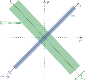
Since the parton is assumed to be propagating in the direction and that it is highly boosted , the dominant component of the parton’s light-cone momentum is . Furthermore, because the parton is highly localised in , the smaller component of the momentum is , i.e., . As consequence, in this regime, the spacetime dependence of the field can be simplified to . In the light-cone gauge (), the background field can be written as . Given the smallness of , the background field can be simplified to have as the only non-zero component, i.e., .
Under the sub-eikonal approximation222The eikonal approximation is usually relaxed to allow small momentum transfers, with the light-cone energy still being conserved, which is known as the sub-eikonal approximation., parton propagation in the medium resembles that of a 2D non-relativistic quantum system. The in-medium scalar propagator of a parton in the transverse plane, from to , is the Green’s function of the Schrödinger equation Blaizot2015
| (1) |
where is a coupling constant. Here, is generically encapsulating both the quark and gluon cases. For the quark case it is defined as
| (2) |
where with the SU(3) generators and ranging from to . Similarly, for the gluon case we have
| (3) |
where are the generators in the adjoint representation, and are the transpose of .
According to Eq. 1, the Hamiltonian that describes the evolution of the parton in the medium is
| (4) |
The first term corresponds to the kinetic energy of the parton, with the light-cone energy playing the role of mass, and the second term corresponds to the potential energy, which is time-dependent. The Hamiltonian rules the evolution of a single parton in the medium, with the subscript for a quark, the subscript for a gluon, and the subscript referring to both cases. The Hamiltonian can be re-written as a function of the light-cone time
| (5) |
This Hamiltonian serves as the foundation for developing a quantum algorithm to simulate the parton’s in-medium propagation.
3 Towards parton evolution in a quantum computer
To study the evolution of a system governed by the Hamiltonian in Eq. 5 in a quantum computer, the time evolution operator needs to be defined. In light-cone coordinates, represents the time dimension in which the medium extends over . Thus, the time evolution operator for the entire medium extension can be written as
| (6) |
This operator acts on a two-dimensional Hilbert space, which is either spanned by the momentum eigenstates or the position eigenstates . The time evolution operator evolves the system along the entire longitudinal extension of the medium, transforming the initial state into a final state . The operator in Eq. 6 can be decomposed non-perturbatively into the sequential product of the same operator but for small time intervals of size , i.e.,
| (7) |
with , , and the number of time steps. In each time step, due to its small size, the time evolution operator can be approximated as the product of the evolution of the kinetic and potential terms. This approximation has corrections of the order of , such that, when , , it becomes exact with the time evolution operator for the whole medium extension being retrieved. This approximation also facilitates mapping the time evolution operator into a quantum circuit.
To implement the evolution on a quantum computer and retrieve information from the final state , the three major steps of the quantum simulation algorithm chuang need to be well-defined as described in the following subsections. The algorithm developed here assumes that the medium probe, the hard parton, is ruled by the SU(3) gauge group, being either a quark or a gluon. The colour degrees of freedom of both quarks and gluons and their Casimir invariants are summarised in Table 1. Furthermore, since the kinetic term of the Hamiltonian is diagonal in the momentum basis, and the potential term is diagonal in the position basis, the algorithm is developed in a mixed representation where the momentum and position bases are both used.
| Gauge Group | Colour degrees of freedom | Casimir invariant | ||
| Quark | Gluon | |||
| SU(3) | ||||
3.1 Embedding and initialization
The system’s data is embedded into quantum states using the basis embedding technique, i.e., the classical bits are directly mapped into quantum bits. For instance, an n-qubit quantum state represents the classical value , where are the classical bits. The two-dimensional Hilbert space essentially corresponds to the two dimensions of the transverse lattice, i.e., and directions. Since the algorithm is developed in a mixed position-momentum basis, the change of basis, between the momentum and position bases, is performed using the Quantum Fourier Transform (QFT) chuang , which is detailed in subsection 3.2.
The transverse lattice is a two-dimensional lattice, with sites per direction with each direction extending from to . The spacing of the lattice is then , in the position basis. Consequently, the lattice spacing in the momentum basis is , which corresponds to the reciprocal lattice spacing. The discrete lattice states and are related to the continuum ones and by
| (8) |
and
| (9) |
A periodic boundary condition is imposed on the lattice, with points separated by an integer multiple of the period being identified:
| (10) |
and
| (11) |
with and a generic operator. This periodic condition identifies the states with with the ones with , and the same for the momentum basis, allowing us to work in the interval for both the position and momentum bases. Working in this interval not only facilitates the basis change through the QFT/QFT†, but also simplifies the basis embedding due to the non-negativity of the indices. Using basis embedding, the system’s state can simply be written
| (12) |
and
| (13) |
where . Consequently, to encode the position/momentum information in the quantum state, we need qubits per direction. The qubits representing the position/momentum form two registers, one for each direction.
Besides the transverse lattice, the system’s state also encodes information about the colour of the parton. The colour of the parton is also embedded using basis embedding, and, for the SU(3) gauge group, when the parton is a quark, there are three possible colours, and so two qubits are needed to encode the colour information, and when the parton is a gluon, three qubits are needed to encode the colour information. The qubits representing the colour form also a register, the colour register. The system’s state is then a tensor product of the transverse lattice state ( or ) and the colour state (), i.e., or .
Regarding the initialization, the transverse lattice is initialised in the zero momentum state, i.e., , unless initial momentum effects are of interest. The colour of the parton is initialised in a uniform superposition.
3.2 Encoding and evolution
After establishing how the system’s data is embedded in quantum states, the time evolution operator in Eq. 6 needs to be discretised and translated into a quantum circuit according to the chosen qubit embedding. Attending to Eq. 7, one only needs to define the time evolution operator for a small time interval , i.e., . Then, the whole time evolution operator is simply the product of these operators. In the context of quantum circuits, this means that one needs to know how to implement the time evolution operator for a small time interval, and then the whole time evolution is simply the sequential application of these operators.
The Hamiltonian defined in Eq. 5 has a time dependence only in the potential term, and so the kinetic operator remains the same in the whole evolution. The time dependence of the potential term arises from the background field. Consequently, to include this time dependence, the background field is sliced into intervals of size . In each slice, the background field is assumed to be constant and is generated in a classical computer. Since the medium is assumed to be constant in each slice , the time steps should not be larger than , i.e., . For a sufficiently small time step , the time evolution operator for each interval can be approximated as the product of the evolution of the kinetic and potential terms, and thus written as
| (14) |
When the parton is a quark, this operator is explicitly written as
| (15) |
and for a gluon
| (16) |
where .
Since the kinetic term is diagonal in the momentum basis and the potential term is diagonal in the position basis, the implementation of the time evolution operator in each step benefits from a mixed space representation: the kinetic operator is applied in the momentum basis; and, the potential operator is applied in the position basis. Although the operator could be applied in other bases, namely only on the momentum or only on the position basis, the mixed space representation is chosen since it promotes a more straightforward quantum implementation. Within the mixed-state representation, in each time step, the evolution operator corresponds then to the implementation of the kinetic term in the momentum basis, the QFT† to change to the position basis, followed by the application of the potential term in the position basis, and, finally, the QFT to change back to the momentum basis. This framework is summarised as a quantum circuit in Figure 2, where the dashed box represents one iteration of the time evolution operator, and the initialization and measurement are also included.
[column sep=0.3cm]
\lstick & \qwbundlen_q \qw \gate[2]U_K\gategroup[3,steps=4,style=dashed,rounded
corners,fill=blue!20, inner xsep=2pt,background] \gateQFT^† \gate[3]U_V \gateQFT \qw … \meter \qw
\lstick \qwbundlen_q \qw \qw \gateQFT^† \qw \gateQFT \qw … \meter \qw
\lstick \qwbundlen_c \gateH \qw \qw \qw \qw \qw … \meter \qw
The implementation of the QFT and QFT† follows the framework described in chuang . The implementation of the kinetic and potential terms is described separately below.
3.2.1 Kinetic term
For each time slice, the time evolution of the kinetic operator is given by
| (17) |
The first step is to implement the square of the momentum operator, i.e., , in the momentum basis where the momentum operator is diagonal, and then exponentiate it. The effect of applying to a momentum state is
| (18) |
Knowing that the lattice momentum states are related to the momentum states by , the effect of applying to a momentum state is
| (19) |
Therefore, the elements of the operator in the momentum basis are determined by
| (20) |
Now, one can directly exponentiate the operator, i.e., with and as fixed parameters, and apply the resulting unitary operator to the momentum states. The creation of a unitary gate from a unitary operator/matrix is done using the UnitaryGate class from the Qiskit library Qiskit2017 .
3.2.2 Potential term
As for the kinetic term, in each time slice, one needs to implement the time evolution operator as a quantum circuit. This operator is given by
| (21) |
for a quark, and
| (22) |
for a gluon.
The potential term is diagonal in the position basis, and so the implementation of the potential term is carried out on this basis. The first step in the implementation of the potential term is to generate the background field on a classical computer, as described in A. Then, the values of the background field need to be contracted with the colour generators for the quark case, or with the structure constants for the gluon case. This contraction can be performed in two different ways, which are both explored and compared. Both methodologies require the representation of the background field as a diagonal matrix in the position basis, denoted as . When the matrix form of the colour generators has a different shape than , where is the number of colour qubits, the matrices should be padded with zeros to achieve the correct shape. The same padding rule applies to the matrices.
The two implementations of colour evolution are as follows:
-
•
The first one consists of contracting the background field with the colour generators or structure constants through a tensorial product, i.e., the matrix form of the background field is tensored with the colour generators or the transpose of the matrix form of the structure constants multiplied by . In this context, being the component of the background field operator in the matrix form, the contraction with the colour generators is given by , and with the matrices is given by . After computing the sum of tensorial products, the resulting operator can be directly done using the UnitaryGate class from the Qiskit library Qiskit2017 , or through the decomposition of the operator into a sum of Pauli strings and then exponentiating the Pauli strings. The resulting operator should act in all the qubits, i.e., the position and colour qubits.
-
•
The second method starts by inferring that the operator can be written as the product of the evolution of each colour component, i.e., with , for the quark, and , for the gluon. Then, the next step consists of verifying that all the matrices and have eigenvalues and . Thus, for each colour component, when the colour state is in the eigenstates with eigenvalue , the operator should be applied on the position qubits, and when the eigenstate has eigenvalue , the operator should be applied on the position qubits. Finally, in this way, the operators are applied through controlled operations, with the colour qubits being the control qubits, and the position qubits being the target qubits. As an example, the implementation of the first colour component of a SU(3) quark can be found in Barata2021 .
3.3 Measurement and post-processing
The last component of the quantum simulation is the measurement. Although one could implement a sophisticated measurement procedure to extract any desired property from the system’s final state – such as the one proposed in Barata2021 to directly extract the jet quenching parameter –, here we chose to retrieve the full probability distribution and then post-process that data. The jet quenching parameter , which is a very relevant quantity in the context of jet quenching, is physically defined as the rate of the transverse momentum broadening Iancu2018 .
By measuring all the qubits, one directly retrieves from the quantum computer the probability distribution of the system’s final state, i.e., the probability of finding the system in each of the possible states. The lattice registers are measured on the momentum basis. Recalling the chosen embedding scheme (subsection 3.1), the measured states are in the form , with being the number of colour qubits. The measured states then need to be post-processed to extract the probability distribution of the squared transverse momentum. This post-processing is done in four major steps:
-
1.
The measured states are converted from the binary representation to the decimal representation;
-
2.
The lattice is recentered, i.e., the values larger than are subtracted by , and so the values are in the range instead of ;
-
3.
The lattice values are converted to the physical values, with the lattice values being multiplied by , i.e., ;
-
4.
The squared transverse momentum is computed, i.e., .
We note that when the colour register is initialised in a uniform superposition containing states without physical meaning, i.e. for a SU(3) quark where two qubits are used to encode the three possible colours, the spurious states should be removed from the momentum distribution and, consequently, the distribution should be renormalised.
To better compare the simulation data with the analytical results, it is convenient to consider the transverse momentum transferred by the medium to the parton, commonly referred to as the saturation scale , which, in the fundamental representation and neglecting logarithmic corrections, is given by
| (23) |
where is the fundamental Casimir of the SU() group.
Besides the direct plots and analysis of the probability distribution, determining the jet quenching parameter and comparing it with the analytical results is also of interest. The jet quenching parameter can be extracted from the probability distributions for different background fields through
| (24) |
where denotes the average over different background field configurations, and denotes the probability weighted average of the squared transverse momentum at the light-front time . When one does not want to study the effect of initial transverse momentum, the initial transverse momentum is set to zero, with the jet quenching parameter being simply given by
| (25) |
The extracted from the simulation is compared with its analytical counterpart, i.e.,
| (26) |
3.4 Discrete lattice effects
The use of a discrete lattice to simulate the parton propagation in a gauge field can lead to undesired lattice effects in the results. These lattice effects can be avoided by the right choice of some of the simulation parameters. Such as in Barata2022 , one is interested in avoiding two main effects: (1) ensuring that the lattice spacing captures all the relevant physics – spacing effects – and (2) ensuring that the assumption that the lattice is finite does not affect the results – finite size effects.
The discrete nature of the lattice introduces two cutoffs, an IR cutoff and an UV cutoff .
To ensure the absence of spacing effects, the lattice spacing should be chosen in such a way that the momentum transfer is much smaller than the UV cutoff , i.e.,
| (27) |
and that the physical IR regulator is much larger than the IR cutoff , i.e.,
| (28) |
Jointly, these two conditions lead to
| (29) |
Due to the lattice periodicity, when there are finite size effects, the lattice edges affect the final momentum distribution by making it asymptotically uniform. Mathematically, a uniform momentum distribution can be described as
| (30) |
Now, defining , to avoid the uniform momentum distribution, one should ensure a set of parameters where , i.e., the total time of the evolution should be smaller than the time needed for the lattice edges to affect the final momentum distribution. For the quark case, recalling the expressions for , Eq. 23, and , Eq. 26, this condition is rewritten as
| (31) |
Consequently, to avoid the finite size effects for a quark, one should ensure that this expression is positive.
For a gluon, the saturation scale is given by and the gluon version of Eq. 31 is obtained by simply replacing .
Spacing effects are avoided for choices of ,, , and , for which Eq. 29 is satisfied.
Figure 3 shows the conditions regarding spacing effects, which are the same for quarks and gluons, for different choices of , , , and . The conditions for finite size effects are shown, separately for quarks and gluons, in Figure 4 and Figure 5.
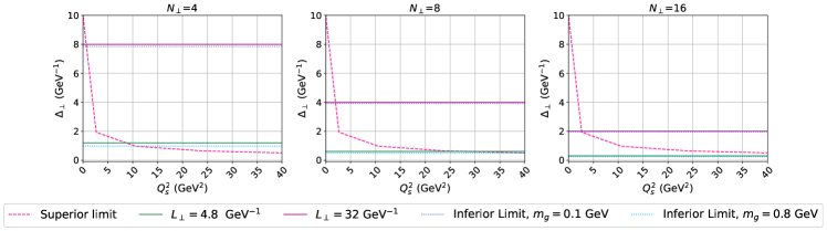
The most salient feature in Figure 3 is that for GeV, using GeV-1 for , leads to spacing effects for all values of and . This is the reason why when GeV-1, GeV is chosen, and when GeV-1, GeV is chosen. Concerning the upper limit, choosing GeV-1 and GeV always allows a larger range of saturation scales that are not affected by spacing effects than choosing GeV-1, . Consequently, the former set of parameters will be used.
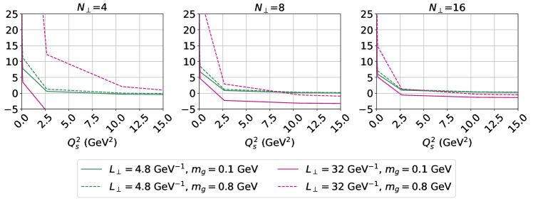
For the quark case, the larger the values of , the smaller the values of that lead to the finite effects, and the larger the values of the larger the values of that lead to the absence of the finite size effects. For GeV-1, the values become “more negative” than for GeV-1, which converge to a small value around as increases. Furthermore, for GeV the lines tend to become negative for smaller values of than for GeV, which is more evident for smaller values of .
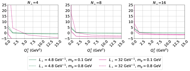
When looking at the results in Figure 5, one can see that the morphology of the curves is quite similar to the ones for the quark case, in Figure 4, with the main and most significant different being the fact that the curves become negative for smaller values of than for the quark case. Consequently, one can expect that the results found for the gluon case are more affected by the finite size effects than the ones for the quark case, especially for the higher values of .
4 Results and analysis
As seen in section 3, SU(3) parton propagation can be performed using different implementations of the potential term: via tensorial product (tensorial method); and via multiple controlled operations (controlled).
For both a SU(3) quark and a SU(3) gluon, one wants to essentially understand the impact of five parameters: , , , and . The first one, , is the number of subdivisions of each medium slice , i.e., for each longitudinal medium slice in how many time steps the quark is evolved, which is closely related to the time step . The other four parameters were already well discussed. The full set of parameters explored in the quantum simulations is presented in Table 2. The only parameters that were a priori chosen to avoid undesired lattice effects are and .
| Parameter (Units) | Value(s) |
|---|---|
| 4, 8, 16 | |
| (GeV-1) | 4.8 |
| 4, 8, 16, 32, 64 | |
| (GeV-1) | 50 |
| (GeV) | 0.004, 0.006, 0.008, 0.01, 0.03, 0.05, 0.06, 0.08, 0.1, 0.5, 1, 1.5, 2 |
| (GeV) | , 200, 100, 50, 5, 1 |
| 1, 2, 4 | |
| (GeV) | 0.8 |
| 1 |
For each study and for each set of parameters, the is calculated from the retrieved momentum distributions, following Eq. 25, and compared to the analytical expectation obtained from Eq. 26. This comparison is always made for different values of and , which is computed with Eq. 23 from the value. Furthermore, for each set of parameters, three different executions of the quantum circuit are performed, corresponding to different background field configurations. Each point in the plot is the mean of the three individual executions and the error bars are their standard deviation.
The decomposition of the quantum operators in quantum gates is always performed using the UnitaryGate class from Qiskit’s framework Qiskit2017 . This choice is made since the majority of the studies performed here are executed in simulation environments and the decomposition of the operators into a sum of Pauli matrices brings additional time to the simulation. Furthermore, due to the large size and depth of the quantum circuits, obtained using both methods, the results using a real quantum device are expected to be severely affected by the noise and the decoherence of the quantum device, and so the use of a more time-consuming method is not justified.
The quantum simulations are implemented using Qiskit’s framework Qiskit2017 . The quantum circuits are almost always executed using the qasm_simulator backend, which is a quantum computer simulator, with the number of shots in each execution being 10000. Due to the actual state of development of quantum devices and their limited access, only a few preliminary quantum simulations were executed in a real quantum device. The simulations were performed on ibm_brisbane device, an Eagle r3 processor, and it was found that the noise completely surpasses the signal, leading to meaningless results. Although this result is not desired, it is expected since error mitigation techniques weren’t used, and the circuits are large and complex.
4.1 Quark
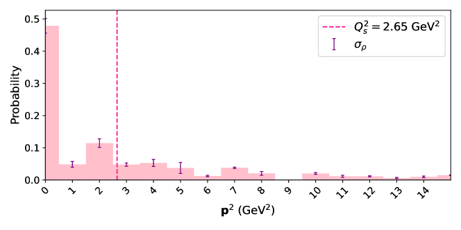
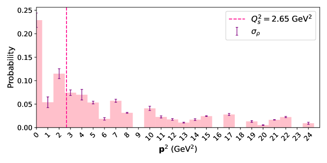
Although not very informative, the first step to analyse the simulation results is to look at the squared momentum distribution retrieved from the quantum computer. The squared momentum distribution for a SU(3) quark with , GeV-1, GeV, , GeV, GeV and is in Figure 6. This figure shows the usual tail-shaped momentum distribution, but, apart from that, it isn’t easy to compare the results with the analytical expectation and analyse them.
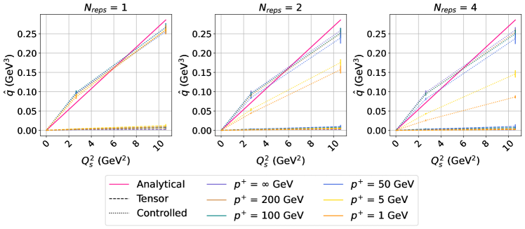
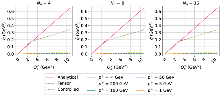
Concerning the impact of the parameter, the same conclusions were always retrieved for the different values of analysed. Therefore, we show in Figure 7 its impact on the jet quenching parameter for several saturation scales, several values of , and the two implementation methods, with , GeV-1, , . The analytical expectation Eq. 26 is also shown for comparison. The increase of the value of leads to worse results, i.e., more distant from the analytical expectation, mainly for smaller values of . Consequently, the value of is fixed to 1 in the other studies. Importantly, only the controlled method is in agreement with the analytical expectation. The discrepancy between the methods should be explained by numerical and simulation errors: the tensorial method implies the tensor product of the colour generators matrices by diagonal matrices representing the colour field values, which are small numbers, leading to a large sparse matrix where the non-zero elements are small numbers; then, this matrix is exponentiated, which adds more numerical errors; and, finally, the matrix needs to be converted into quantum gates, which is a process that relies on approximations, introducing more errors. In comparison, the controlled method only requires exponentiating the matrices representing the colour generators component by component and then converting them into quantum gates, which is a much simpler procedure.
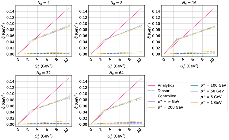
Even though the impact of the parameter was studied for different values of , the considered values of are different for each given . The larger the and m the slower and more resource consuming are the simulations. Although increasing the value leads to convergent results respecting the different values, the convergence for small values of makes the improvement difficult to see in Figure 8, Figure 9 and Figure 10.
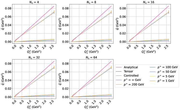
When comparing different values, one can easily infer that the larger the value, the larger the range of saturation scales that lead to results in a good agreement with the classical expectation. This result is explained by the spacing effects present in the simulations (see Figure 3).
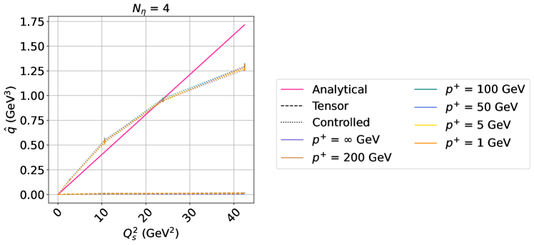
4.2 Gluon
The analysis of the results for the gluon case follows closely the quark case, leading to similar conclusions. Figure 11 shows squared momentum distribution for gluon.
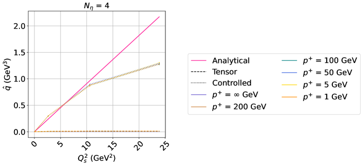
The impact of on the jet quenching parameter is shown in Figure 12, including comparison with the analytical expectation, Eq. 26. Noteworthy is that saturation scale range for which we found a good agreement with the analytical expectation is smaller than for the quark case due to more significant discrete lattice effects.
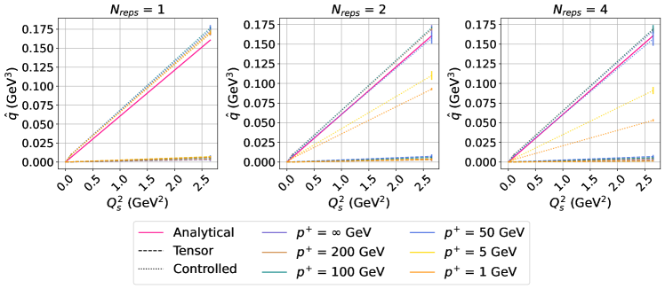
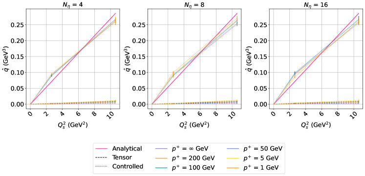
Figure 13, Figure 14, and Figure 15 show the impact of different choices of on the jet quenching parameter. Again, the reduced range of saturation scales for which there is agreement with the analytical baseline is explained by more significant discrete lattice effects for gluons than for quarks.
5 Conclusions
This work investigated the feasibility of simulating the evolution of jets in a quantum computer, more precisely, the propagation of a single SU(3) parton through a medium. The results obtained, for both the quark and gluon cases, were analised and compared against the classical expectation and discussed.
In a quantum simulation environment, the results closely matched analytical expectations for saturation scales below approximately GeV2, demonstrating the potential of using quantum computers to simulate and solve this class of problems.
We found that the longitudinal evolution should be divided into as many steps as the ones of the division of the longitudinal background medium. When the longitudinal evolution is divided into more steps than the background medium ones, there is a decrease in performance. Furthermore, more divisions of the background field lead to better results, especially for smaller values of . Although some preliminary tests for SU(2) partons have shown that the controlled and tensorial methods have similar performances, for the physical meaningful theory – the SU(3) – the performance of the tensorial method vanishes.
Even though the results obtained in this work are promising, there are still many challenges to overcome. The most immediate extension of this work involves extending the Fock space to better approximate the full evolution of jets333 Although in Barata2023 the Fock space was already extended to include the gluon production, the simulation was performed for a very simple case with . Therefore, the next major step in this direction is to extend the Fock space using lattices and saturation scales similar to those employed here.. Another direction to follow in the future relates to the interaction with the medium. The quantum nature of the quark-gluon plasma makes the integration of the medium generation/simulation in the quantum algorithm itself a very interesting next step. Designing a procedure to simulate the entire interaction with the medium on a quantum computer would allow for a full quantum simulation of jet evolution. This full quantum regime would likely be more advantageous when fault-tolerant quantum computers become available. Furthermore, the natural representation of the SU(3) group would be a unit of information with three different states, one for each colour. From the quantum information perspective, this would involve a qutrit gokhale2020 ; Roy_2023 or a hybrid qubit-qutrit Bakkegaard_2019 representation. Finally, the proposed algorithm is expected to be improvable by exploring quantum error mitigation techniques Cai2023 ; Temme2017 ; van_den_Berg_2023 ; Wallman_2016 . It should be remarked, nonetheless, that even if this is a promising path, it is not foreseeable that such error mitigation techniques will drastically improve the current results in a near future, due to the high dimensionality of the circuits.
In conclusion, this work, along with other studies Barata2021 ; Barata2022 ; Barata2023 , represents one of the first steps on the long road towards simulating the full evolution of jets on a quantum computer. Even though the results demonstrate the feasibility of the quantum simulation of the jet evolution, there are still challenges to overcome and many steps to follow to achieve a full simulation of jets in a quantum computer.
Acknowledgements.
We would like to thank João Barata and Carlos Salgado for the relevant and interesting meetings and all the helpful information. We would also like to thank Ricardo Ribeiro and José Rufino for kindly providing access to some of the computing systems used in this work. We acknowledge the use of IBM Quantum services for this work. This work was produced with the computational support of INCD funded by FCT and FEDER under the project with reference 2023.10635.CPCA.A1. This work was financed by national funds through FCT ‑ Fundação para a Ciência e a Tecnologia, I.P., within the scope of the project CERN/FIS‑ PAR/0032/2021 and by European Research Council (ERC) under the European Union’s Horizon 2020 research and innovation programme (Grant agreement No. 835105, YoctoLHC).Appendix A colour background field
The statistics of the colour background field are described by a version of the McLerran-Venugopalan model McLerran1994 ; McLerran1994v2 that assumes that the colour charges of the medium are correlated white-noise statistics, just as assumed in Barata2022 ; Barata2023 . Hence, the colour background field is a classical stochastic field, which satisfies the reduced Yang-Mills equations,
| (32) |
where is the gluon mass, introduced to regularise the infrared divergence, ensuring the colour neutrality of the source distribution Krasnitz2003 , and is the colour charge density describing the medium’s energetic degrees of freedom. The colour charge density is assumed to have a Gaussian correlation function, i.e.,
| (33) |
where denotes the average over different medium configurations, is the QCD coupling constant, and has dimension of GeV and can be interpreted as the medium’s density of scattering centres and so determines the strength of the parton-medium interaction. In the context of high-energy scattering processes, the charge density is usually integrated over the longitudinal extension of the medium. This new quantity is known is the saturation scale defined in Eq. 23.
By solving Eq. 32, the background field can finally be expressed as
| (34) |
Appendix B Analytical jet quenching parameter
The first step to compute the analytical jet quenching parameter is to rewrite Eq. 24 as
| (35) |
where is the initial state of the system, and is the usual time evolution operator from the light-front time to the light-front time , i.e., for the whole medium. Through a Fourier transform, the in coordinate space is given by
| (36) |
where is the directional derivative along , and is a Wilson line along in the light-cone framework which can be explicitly written as
| (37) |
and corresponds to the evolution operator (Eq. 6) in the eikonal limit, i.e., 444In Blaizot2013 is shown that assuming finite values, and so, including the kinetic term at the leading eikonal order, does not affect the .. For the quark case, the above Wilson line should be used in the fundamental form, i.e., should be replaced by , and for the gluon case, the adjoint form, i.e., replaced by .
By choosing coincident coordinates , and substituting the Wilson line (Eq. 37) in the expression for , one obtains
| (38) |
In Eq. 37, the Wilson line is explicitly written in the fundamental form for the quark case, and, if one wants to analyze the gluon case, one should replace the fundamental matrices with the adjoint ones. Now, by using the background field definition (Eq. 34) and by omitting the colour indices for simplicity, the for a quark can be rewritten as
| (39) |
Now, remembering the colour charge density correlator (Eq. 33), one can write
| (40) | ||||
For the gluon case, the matrices should be replaced by the matrices, i.e.,
| (41) |
Finally, including the result in Eq. 40 in the expression for , one obtains
| (42) | ||||
The discrete nature of the transverse lattice introduces two momentum cutoffs, which are the Infra-Red (IR) and the Ultra-violet (UV) cutoffs, and which are defined as and , respectively. Thus, the above integral can be rewritten in polar coordinates, with the module of , as
| (43) | ||||
References
- (1) G.P. Salam, The European Physical Journal C 67(3–4), 637–686 (2010). DOI 10.1140/epjc/s10052-010-1314-6
- (2) U.A. Wiedemann, Jet Quenching in Heavy Ion Collisions (Springer Berlin Heidelberg, 2010), p. 521–562. DOI 10.1007/978-3-642-01539-7˙17. URL http://dx.doi.org/10.1007/978-3-642-01539-7_17
- (3) A. Majumder, M. van Leeuwen, Progress in Particle and Nuclear Physics 66(1), 41–92 (2011). DOI 10.1016/j.ppnp.2010.09.001. URL http://dx.doi.org/10.1016/j.ppnp.2010.09.001
- (4) Y. Mehtar-Tani, J.G. Milhano, K. Tywoniuk, International Journal of Modern Physics A 28(11), 1340013 (2013). DOI 10.1142/s0217751x13400137
- (5) J.P. Blaizot, Y. Mehtar-Tani, International Journal of Modern Physics E 24(11), 1530012 (2015). DOI 10.1142/s021830131530012x
- (6) G.Y. Qin, X.N. Wang, International Journal of Modern Physics E 24(11), 1530014 (2015). DOI 10.1142/s0218301315300143. URL http://dx.doi.org/10.1142/S0218301315300143
- (7) L. Apolinário, Y.J. Lee, M. Winn, Progress in Particle and Nuclear Physics 127, 103990 (2022). DOI 10.1016/j.ppnp.2022.103990. URL http://dx.doi.org/10.1016/j.ppnp.2022.103990
- (8) I.P. Lokhtin, A.M. Snigirev, Journal of Physics G: Nuclear and Particle Physics 34(8), S999–S1003 (2007). DOI 10.1088/0954-3899/34/8/s143
- (9) N. Armesto, L. Cunqueiro, C.A. Salgado, Eur. Phys. J. C 63, 679 (2009). DOI 10.1140/epjc/s10052-009-1133-9
- (10) K. Zapp, The European Physical Journal C 74(2) (2014). DOI 10.1140/epjc/s10052-014-2762-1
- (11) J. Casalderrey-Solana, D.C. Gulhan, J.G. Milhano, D. Pablos, K. Rajagopal, Journal of High Energy Physics 2014(10) (2014). DOI 10.1007/jhep10(2014)019
- (12) J.H.P. et al. The jetscape framework (2019)
- (13) S.J. Freedman, J.F. Clauser, Phys. Rev. Lett. 28, 938 (1972). DOI 10.1103/PhysRevLett.28.938
- (14) A. Aspect, J. Dalibard, G. Roger, Phys. Rev. Lett. 49, 1804 (1982). DOI 10.1103/PhysRevLett.49.1804
- (15) J. Preskill, Quantum 2, 79 (2018). DOI 10.22331/q-2018-08-06-79
- (16) J. Barata, C. Salgado, The European Physical Journal C 81 (2021). DOI 10.1140/epjc/s10052-021-09674-9
- (17) J. Barata, X. Du, M. Li, W. Qian, C.A. Salgado, Phys. Rev. D 106, 074013 (2022). DOI 10.1103/PhysRevD.106.074013
- (18) J. Barata, X. Du, M. Li, W. Qian, C.A. Salgado, Phys. Rev. D 108, 056023 (2023). DOI 10.1103/PhysRevD.108.056023
- (19) M.A. Nielsen, I.L. Chuang, Quantum Computation and Quantum Information: 10th Anniversary Edition (Cambridge University Press, 2011)
- (20) Qiskit Community. Qiskit: An open-source framework for quantum computing (2017). DOI 10.5281/zenodo.2562110. URL https://github.com/Qiskit/qiskit
- (21) E. Iancu, P. Taels, B. Wu, Physics Letters B 786, 288 (2018). DOI 10.1016/j.physletb.2018.10.007
- (22) P. Gokhale, J.M. Baker, C. Duckering, F.T. Chong, N.C. Brown, K.R. Brown, IEEE Micro 40, 64 (2020). DOI 10.1109/MM.2020.2985976
- (23) T. Roy, Z. Li, E. Kapit, D.I. Schuster, Phys. Rev. Appl. 19, 064024 (2023). DOI 10.1103/PhysRevApplied.19.064024
- (24) T. Bækkegaard, L.B. Kristensen, N.J.S. Loft, C.K. Andersen, D. Petrosyan, N.T. Zinner, Scientific Reports 9(1) (2019). DOI 10.1038/s41598-019-49657-1
- (25) Z. Cai, R. Babbush, S.C. Benjamin, S. Endo, W.J. Huggins, Y. Li, J.R. McClean, T.E. O’Brien, Rev. Mod. Phys. 95, 045005 (2023). DOI 10.1103/RevModPhys.95.045005
- (26) K. Temme, S. Bravyi, J.M. Gambetta, Phys. Rev. Lett. 119, 180509 (2017). DOI 10.1103/PhysRevLett.119.180509
- (27) E. van den Berg, Z.K. Minev, A. Kandala, K. Temme, Nature Physics 19(8), 1116–1121 (2023). DOI 10.1038/s41567-023-02042-2
- (28) J.J. Wallman, J. Emerson, Physical Review A 94(5) (2016). DOI 10.1103/physreva.94.052325
- (29) L. McLerran, R. Venugopalan, Physical Review D 49(7), 3352 (1994). DOI 10.1103/physrevd.49.3352
- (30) L. McLerran, R. Venugopalan, Physical Review D 49(5), 2233 (1994). DOI 10.1103/physrevd.49.2233
- (31) A. Krasnitz, Y. Nara, R. Venugopalan, Nuclear Physics A 717(3), 268 (2003). DOI https://doi.org/10.1016/S0375-9474(03)00636-5
- (32) J. Blaizot, F. Dominguez, E. Iancu, Y. Mehtar-Tani, Journal of High Energy Physics 2013(1) (2013). DOI 10.1007/jhep01(2013)143