Estimating causal effects using difference-in-differences under network dependency and interference

Abstract

Differences-in-differences (DiD) is a causal inference method for observational longitudinal data that assumes parallel expected outcome trajectories between treatment groups under the (possible) counterfactual of receiving a specific treatment. In this paper DiD is extended to allow for (i) network dependency where outcomes, treatments, and covariates may exhibit between-unit latent correlation, and (ii) interference, where treatments can affect outcomes in neighboring units. In this setting, the causal estimand of interest is the average exposure effect among units with a specific exposure level, where the exposure is a function of treatments from potentially many units. Under a conditional parallel trends assumption and suitable network dependency conditions, a doubly robust estimator allowing for data-adaptive nuisance function estimation is proposed and shown to be consistent and asymptotically normal with variance reaching the semiparametric efficiency bound. The proposed methods are evaluated in simulations and applied to study the effects of adopting emission control technologies in coal power plants on county-level mortality due to cardiovascular disease.

Keywords: average treatment effect on the treated, dependent data, difference-in-differences, double robustness, parallel trends, policy evaluation, semiparametric theory

1 Introduction

1.1 Background

Differences-in-differences (DiD) is a popular causal inference method to estimate causal effects in observational studies that relies on a parallel trends assumption. Under the canonical set-up with a treatment indicator and pre- and post-treatment time periods, the parallel trends assumption stipulates that the average outcome in the treated and untreated groups would have changed by the same amount post-treatment, under the scenario where neither group received the treatment [1]. DiD allows for the identification and estimation of causal effects in the absence of treatment randomization and has been used to estimate the effects of various treatments, exposures, and policies such as contaminated water on cholera incidence [2], minimum wage laws on unemployment [3], employment protection on productivity [4], and Medicare on mortality and medical spending [5], among many other applications across fields.

Challenges to estimation and inference may occur when data are dependent. For instance, when evaluating place-based policy interventions, there may be interference where a policy enacted in one unit (e.g., a county or state) may have effects in neighboring units. The type of interference varies by study and includes clustered interference where dependency between treatments and potential outcomes may occur within clusters but not between clusters, and network interference where possible dependency is described by network ties. Additionally, outcomes of units that are close in geographic space or within a network may exhibit latent variable dependence where outcomes in one unit are correlated with outcomes from neighboring units through shared unobserved variables. For example, health outcomes (e.g., all-cause mortality) measured at the county level may be correlated across counties due to unobserved environmental pollutants that affect neighboring counties similarly. Latent variable dependence may also be present for covariates and treatments. In studies of social networks, correlation between person-level data is often exhibited through homophily, where peers connected in a social network tend to share similar characteristics. Certain data settings may exhibit interference, latent variable dependence, both, or neither. For a more extensive discussion of correlation and interference from a spatial perspective, see Papadogeorgou and Samanta [6]. Most causal inference methods assume independent and identically distributed (iid) data, implying that neither interference nor latent variable dependence occur.

In addition to non-iid data, in some settings another challenge is posed where outcomes and treatments are measured on different units. The bipartite interference setting considers outcomes and treatments measured on different types of units and where multiple treatment units may affect the potential outcomes of each outcome unit [7]. Bipartite interference is particularly relevant in environmental health since outcome data is often defined on the person-level (or some aggregate, such as the census tract or county level) while interventions are performed on the environment; for example, regulations on air or water quality. Outside of environmental health, the bipartite structure may be present when the intervention target is a spatial unit. Causal estimands of interest under bipartite interference may differ from estimands in the standard interference setting since under the bipartite setting, there may not be a single treatment unit tied to a particular outcome unit, complicating the definitions of the commonly studied direct and spillover effects.

In the motivating data application for this paper, the treatment is the implementation of flue-gas desulfurization scrubbers in coal power plants. Coal power plants emit sulfur dioxide (SO₂) which interacts with the atmosphere and breaks down to particular matter less than 2.5 microns in diameter (PM2.5). Recent studies have provided evidence that exposure to PM2.5 may cause increased risk of some cardiovascular diseases (CVDs) (see, e.g., Wu et al. [8]). Scrubbers are an emission control technology that help limit the amount of SO₂ emitted. Bipartite interference may be present since intervention and outcome units differ and atmospheric conditions (e.g., weather patterns) can move emissions across counties such that the CVD mortality rate for a particular county may depend on scrubber installation in a distant power plant located in a different county.

In this paper, the doubly robust DiD estimator proposed by Sant’Anna and Zhao [9] for iid data is adapted to the network dependent data setting with (bipartite) interference. Sufficient conditions for consistency and asymptotic normality of the estimator are shown. Data dependency is modeled by networks, and inference relies on asymptotics that allow for certain types of network dependencies. The proposed methods are utilized to study the effects of an air pollution control technology on county-level mortality rate due to CVDs. Although the data application exhibits the bipartite structure, all statistical results in this study include the non-bipartite setting as a special case.

The remainder of this paper is organized as follows. Related work is reviewed in Section 1.2. Section 2 introduces notation, defines the causal estimand of interest, provides assumptions sufficient to identify the causal estimand, proposes estimators, and derives the large sample properties of the proposed estimators. Section 3 evaluates properties of the proposed estimators under simulated finite samples. Section 4 applies the proposed methods to the motivating data application. Finally, Section 5 concludes and discusses future work.

1.2 Related work

This study builds on recent methodological work studying DiD, interference, and dependent data limit theorems. At the intersection of DiD and interference, several studies assumed two-way fixed effects (TWFE) models where the outcome is assumed have a known structural relationship with treatments after adjusting for individual and time fixed effects [10, 11, 12]. Hettinger et al. [13] and Lee et al. [14] considered an exposure mapping specific for their motivating data application that reduced potential outcomes to the canonical DiD setting, motivating outcome regression (OR), inverse probability weighted (IPW), and doubly robust (DR) estimators. Shahn et al. [15] derived structural nested mean models under parallel trends allowing for clustered or network interference. Xu [16] considered DiD from a finite-population perspective and assumed an exposure mapping with approximate neighborhood interference, where interference is assumed to be limited and decaying outside of neighborhoods. Xu proposed a generalized method of moments estimator and derived sufficient conditions for the estimator to reach the semiparametric efficiency bound under parametric estimation of nuisance functions.

In the iid setting, Sant’Anna and Zhao [9] proposed a semiparametric doubly robust estimator of the average treatment effect on the treated under a conditional parallel trends assumption. The proposed estimator was shown to be semiparametric efficient, consistent, and asymptotically normal under parametric estimation of nuisance functions.

Kojevnikov et al. [17] proposed a law of large numbers and a central limit theorem for dependent data under suitable network dependency conditions. Leung [18] employed the limit theorems of Kojevnikov et al. to show consistency and asymptotic normality of an inverse-probability weighted estimator of causal effects where interference may be present.

In contrast to previous work involving DiD under interference, this paper considers the conditional parallel trends assumption, simultaneously accommodates network interference and latent variable dependency, and proposes a nonparametric doubly robust estimator that allows for data-adaptive estimation of nuisance functions and is CAN under suitable conditions. The proposed methods also allow for bipartite interference.

Conditional parallel trends and an exposure mapping from all intervention unit treatments to a discrete scalar are assumed. Potential outcomes are allowed to depend on their exposure history, and the proposed estimand includes as a special case other recently proposed estimands for the staggered treatment adoption setting, e.g., Callaway and Sant’Anna [19]. These methods are applied to estimate the effect of installing scrubbers in coal power plants on county-level mortality due to cardiovascular diseases.

2 Methods

2.1 Notation and potential outcomes

Considering the setting where there may be bipartite interference, let $i=1,\dots,n$ index the outcome units and $j=1,\dots,m$ index the intervention (treatment) units. In the data application below, $i$ indexes counties and $j$ indexes power plants. The non-bipartite setting is a special case where $i=j$ and $n=m$. Time periods are indexed $t=0,\dots,T$ where $t=0$ is a pre-treatment period for all units. At time $t$, intervention unit $j$ receives treatment $Z_{jt}$ which may be multi-valued or continuous. Let $z_{jt}$ denote realizations of $Z_{jt}$ and $z_{jt}\in\mathcal{Z}\subseteq\mathbb{R}$. Throughout this paper, the notation is adopted that for an arbitrary time-varying variable $Q_{it}$, boldface denotes the vector across (either outcome or intervention) units, e.g., $\mathbf{Q}_{t}=(Q_{1t},\dots,Q_{nt})^{\mathrm{T}}$ and overbars denote histories, e.g., $\mathbf{\bar{Q}}_{t}=(\mathbf{Q}_{1},\dots,\mathbf{Q}_{t})_{n\times t}$ and $\mathbf{\bar{Q}}_{s:t}=(\mathbf{Q}_{s},\dots,\mathbf{Q}_{t})_{n\times(t-s+1)}$.

The potential outcomes for the outcome units are defined on the entire treatment history for the study period and are denoted by $Y_{it}(\mathbf{\bar{z}}_{T})$ where $\mathbf{\bar{z}}_{T}$ is the $m\times(T+1)$ matrix of treatment histories for all $m$ intervention units up to time $T$. Note that since $t=0$ is the pre-treatment period for all units, $\mathbf{Z}_{0}=\mathbf{0}$. To relate potential outcomes to observed outcomes, the following form of causal consistency is assumed.

Assumption 1 (Causal consistency).

If $\mathbf{\bar{Z}}_{T}=\mathbf{\bar{z}}_{T}$, then $Y_{it}=Y_{it}(\mathbf{\bar{z}}_{T})$.

The proposed methods rely on an assumption about the interference structure between outcome and treatment units. Let $W_{t}$ be the $n\times m$ matrix of interference weights with elements $w_{ijt}\in[0,1]$ that describe the amount of potential interference of the $j$th intervention unit to the $i$th outcome unit at time $t$. In the case when $w_{ijt}\in\{0,1\}$, possible interference is denoted by $w_{ijt}=1$ while $w_{ijt}=0$ implies no interference. However, in certain studies, there may be prior knowledge that some intervention units are more influential than others with respect to a particular unit’s potential outcome. For example, in the motivating air pollution study, treatments at power plants in closer proximity to a particular county are reasonably assumed to be more influential to that county’s CVD mortality rate compared to further away power plants. In these settings, specifying $w_{ijt}\in[0,1]$ allows higher values of $w_{ijt}$ to reflect greater relative influence where $w_{ijt}=0$ still denotes no interference.

The interference set for outcome unit $i$ at time $t$ is defined as $\mathcal{I}_{it}=\{j:w_{ijt}\neq 0\}$, i.e., the collection of intervention units that have non-zero interference weights with outcome unit $i$. Define an exposure mapping to be a surjective function from the vector of treatments for all intervention units at time $t$ and the vector of interference weights for unit $j$ to a bounded real scalar, i.e., $g(\mathbf{Z}_{t};\mathbf{w}_{it}):\mathcal{Z}^{m}\times[0,1]^{m}\rightarrow\mathcal{G}$ where $\mathcal{G}$ is a discrete set and $\mathbf{w}_{it}=(w_{i1t},\dots,w_{ijt},\dots,w_{imt})$. Many common exposure mappings can be expressed as functions of an interference matrix; for example, the (weighted) proportion of neighbors that were treated corresponds to $g(\mathbf{Z}_{t};\mathbf{w}_{it})=\sum_{j\in\mathcal{I}_{it}}w_{ijt}Z_{jt}\big{/}\sum_{j\in\mathcal{I}_{it}}w_{ijt}$. Ideally, specification of the exposure mapping function and interference matrix would be derived from domain-specific knowledge. For instance, in the data example, air pollution from power plants can affect county-level health if weather patterns move the pollution from a specific power plant to a county. Thus, an atmospheric transport model was used to specify $W_{t}$; see Section 4 for more details. For convenience, let $G_{it}:=g(\mathbf{Z}_{t};\mathbf{w}_{it})$ denote the random exposure for outcome unit $i$ at time $t$. Also, with a slight abuse of notation, let $\bar{g}(\mathbf{\bar{z}}_{t};\mathbf{\bar{w}}_{it})=(g(\mathbf{z}_{1};\mathbf{w}_{it}),\dots,g(\mathbf{z}_{t};\mathbf{w}_{it}))^{\mathrm{T}}$. Further, let the random exposure histories be denoted $\bar{G}_{t}$ and realizations be denoted $\bar{g}_{t}$.

Assumption 2 (Interference through exposure mapping).

For any $\mathbf{\bar{Z}}_{T}=\mathbf{\bar{z}}_{T}$, $\mathbf{\bar{Z}}_{T}=\mathbf{\bar{z}}^{\prime}_{T}$ such that $\bar{g}(\mathbf{\bar{z}}_{T};\mathbf{\bar{w}}_{iT})=\bar{g}(\mathbf{\bar{z}}^{\prime}_{T};\mathbf{\bar{w}}_{iT})$, the following equality holds for all $i=1,\dots,n$ and $t=0,\dots,T$: $Y_{it}(\mathbf{\bar{z}}_{T})=Y_{it}(\mathbf{\bar{z}}^{\prime}_{T})$.

Assumption 2 stipulates that potential outcomes are based on the amount of exposure as defined by the exposure mapping and therefore can be expressed in terms of the exposure histories $Y_{it}(\bar{g}_{T})$. This notation is adopted for the remainder of the paper unless otherwise stated. The distribution of the potential outcomes $Y_{it}(\bar{g}_{T})$ depends implicitly on the interference matrix $W_{t}$, which further implies dependency on $n$ and $m$. Further note that $Y_{it}(\bar{g}_{T})$ is defined only when each element of $\bar{g}_{T}$ is in the set $\mathcal{G}$.

Each outcome and intervention unit has associated $p\times 1$ and $q\times 1$ pre-treatment covariates $X_{i}^{\mathrm{out}},i=1,\dots,n$ and $X_{j}^{\mathrm{int}},j=1,\dots,m$, respectively. Let the collection of baseline outcome and intervention unit covariates associated with outcome unit $i$ be denoted $X_{i}=(X_{i}^{\mathrm{out}},s(\{X_{j}^{\mathrm{int}}\}_{j\in\mathcal{I}_{i0}}))$ where $s(\cdot)$ is a user-specified function that maps intervention unit covariates to a potentially low dimensional space that does not depend on $i$. When there are many intervention units in the interference set of each outcome unit at time $0$, the dimensionality of $\{X_{j}^{\mathrm{int}}\}_{j\in\mathcal{I}_{i0}}$ may potentially be very large. In these high dimensional settings, the function $s(\cdot)$ may be useful to reduce dimensionality. For instance, one may consider a weighted average of intervention unit covariates with weights according to the interference matrix.

For each outcome unit, the random data vector $O_{i}=(\bar{Y}_{iT},\bar{G}_{iT},\{\mathbf{\bar{Z}}_{jT}\}_{j\in\mathcal{I}_{i}},X_{i})$ is observed where $\mathcal{I}_{i}=\cup_{t=1}^{T}\mathcal{I}_{it}$. Henceforth, the $i$ subscript will be suppressed unless needed for clarity. The dependency between data will be modeled using networks to allow for asymptotic inference; these network models will be described in detail in Section 2.4. Throughout this paper, all estimands and estimators implicitly condition on the sample sizes $n$, $m$, and the network, i.e., randomness from the network generating process is not considered. The motivating example presented in Section 4 uses data from the network of power plants and counties in the United States, which is the population of interest. In settings such as the study of social networks where the network is a sample from a larger network, additional assumptions may be needed for inference about the target population; see Ogburn et al. [20] for discussion.

2.2 Causal estimand

The causal estimand of interest is an analogue to the average treatment effect on the treated for this setting with an exposure mapping and time-varying treatments. In particular, define the average exposure effect on the exposed (AEE) to be:

$$\tau\coloneqq\operatorname{AEE}_{t,\delta}(\bar{g}_{t},\bar{g}^{\prime}_{t})=\mathrm{E}\left[Y_{it}(\bar{g}_{t})-Y_{it}(\bar{g}_{t}^{\prime})|\bar{G}_{it}=\bar{g}_{t}\right],$$

where $\bar{g}_{t}=(\bar{g}_{t-\delta},\bar{g}_{(t-\delta+1):t})$, $\bar{g}_{t}^{\prime}=(\bar{g}_{t-\delta},\bar{g}_{(t-\delta+1):t}^{\prime})$, and $1\leq\delta\leq t$ for $\bar{g}_{(t-\delta+1):t}\neq\bar{g}_{(t-\delta+1):t}^{\prime}$. In words, $\tau$ is the average effect at time $t$ of an exposure history $\bar{g}_{t}$ relative to another exposure $\bar{g}_{t}^{\prime}$ among those receiving exposure $\bar{g}_{t}$. The estimand $\tau$ is essentially a “blip” function among the group with exposure $\bar{g}_{t}$, so-named since it compares potential outcomes under the same exposure history up to time $t-\delta$ but differing thereafter. If $\delta$ is set to $1$, the estimand isolates the effect of a change in exposure in the time period $t$. $\operatorname{AEE}_{t,\delta}(\bar{g}_{t},\bar{g}_{t}^{\prime})$ reduces to the classic average treatment effect on the treated when there is no interference, two time periods, two treatments $z\in\{0,1\}$, and $\bar{g}_{t}=(0,1)$ and $\bar{g}_{t}^{\prime}=(0,0)$. Estimand 2.2 also reduces to the group-time average treatment effect parameter introduced in Callaway and Sant’Anna [19] when there are two treatments and $\bar{g}_{t}^{\prime}=(0,\dots,0)$ and $\bar{g}_{t}=(0,\dots,0,1,\dots,1)$ where the timing of the change from $0$ to $1$ in $\bar{g}_{t}$ is specified.

2.3 Identification and estimation

In this section, the AEE is shown to be identifiable under Assumptions 1-2 and the following three assumptions of no anticipation, positivity, and conditional parallel trends. No anticipation in Assumption 3 states that potential outcomes at time $s$ do not depend on treatments at times $t>s$. In other words, potential outcomes do not vary based on treatments occurring in the future. Accordingly, potential outcomes at time $t$ can be written as depending on treatment history up to time $t$ only, i.e., $Y_{it}(\mathbf{\bar{z}}_{t})$ or $Y_{it}(\bar{g}_{t})$ under Assumption 2.

Assumption 3 (No anticipation).

Let $\mathbf{\bar{z}}_{T}=(\mathbf{\bar{z}}_{t},\mathbf{\bar{z}}_{(t+1):T})$, then $Y_{it}(\mathbf{\bar{z}}_{T})=Y_{it}(\mathbf{\bar{z}}_{t},\mathbf{\bar{z}}_{(t+1):T}^{\prime})$ for any $\mathbf{\bar{z}}_{(t+1):T}^{\prime}$.

Under Assumption 4, the two exposure histories being compared in the causal estimand must have a positive probability of occurring. Note that a similar positivity assumption on the intervention unit treatments $\mathbf{Z}$ is not needed.

Assumption 4 (Positivity of exposure history).

There exists $\epsilon>0$ such that

$$\mathrm{P}(\bar{G}_{t}=\bar{g}_{t}|X)>\epsilon \text{ and }\mathrm{P}(\bar{G}_{t}=\bar{g}_{t}^{\prime}|X)>\epsilon,$$

$$\mathrm{P}(\bar{G}_{t}=\bar{g}_{t})>\epsilon \text{ and }\mathrm{P}(\bar{G}_{t}=\bar{g}_{t}^{\prime})>\epsilon.$$

The conditional parallel trends assumption in Assumption 5 states that the path of potential outcomes under the reference exposure $\bar{g}_{t}^{\prime}$ is the same, in expectation, for the group with treatment history $\bar{g}_{t}$ and the group with exposure history $\bar{g}_{t}^{\prime}$, conditional on covariates. Recall that the two comparison exposure groups have the same treatment history up to time $t-\delta$ but differ from time $t-\delta+1$ to $t$ if $\bar{g}_{(t-\delta+1):t}\neq\bar{g}_{(t-\delta+1):t}^{\prime}$. Thus, covariates that satisfy conditional parallel trends are those that affect both the potential outcome trajectory under $\bar{g}_{t}^{\prime}$ and exposure sequences. For instance, in the power plant example, for a particular county, median income may affect both mortality trends and the probability that a power plant in that county installs a scrubber.

Assumption 5 (Conditional parallel trends).

For all $i=1,\dots,n$,

$$\mathrm{E}[Y_{t}(\bar{g}^{\prime}_{t})-Y_{t-\delta}(\bar{g}^{\prime}_{t})|X,\bar{G}_{t}=\bar{g}^{\prime}_{t}]=\mathrm{E}[Y_{t}(\bar{g}^{\prime}_{t})-Y_{t-\delta}(\bar{g}^{\prime}_{t})|X,\bar{G}_{t}=\bar{g}_{t}].$$

Note that if there are two time periods $t\in\{0,1\}$, and the exposures are $g_{1}^{\prime}=0$, $g_{1}=1$, and $\mathcal{G}_{1}=\{0,1\}$, then this assumption reduces to the classic conditional parallel trends assumption as in Abadie [21]. In practice, one may choose to restrict this assumption for a specific $g^{\prime}$ such as $g^{\prime}=0$ or $g^{\prime}=\min_{g}\{g:g\in\mathcal{G}\}$. When $g^{\prime}=0$, the parallel trends assumption would be the same as that made in Callaway and Sant’Anna [19].

In DiD studies, usually the conditional parallel trends assumption is only made with respect to the reference treatment (exposure) group $\bar{G}=\bar{g}_{t}^{\prime}$, which identifies the ATT (AEE). However, if the conditional parallel trends assumption can also be made with respect to $\bar{G}=\bar{g}_{t}$, i.e., $\mathrm{E}[Y_{t}(\bar{g}_{t})-Y_{t-\delta}(\bar{g}_{t})|X,\bar{G}_{t}=\bar{g}_{t}]=\mathrm{E}[Y_{t}(\bar{g}_{t})-Y_{t-\delta}(\bar{g}_{t})|X,\bar{G}_{t}=\bar{g}_{t}]$, then the unconditional treatment (exposure) effect $\mathrm{E}\left[Y_{it}(\bar{g}_{t})-Y_{it}(\bar{g}_{t}^{\prime})\right]$ would also be identified.

The causal estimand $\operatorname{AEE}_{t,\delta}(\bar{g},\bar{g}^{\prime})$ is identifiable under the above assumptions. Let $\mu_{\bar{g}_{t}}(x):=\mathrm{E}[Y_{t}|X=x,\bar{G}_{t}=\bar{g}_{t}]$ be the true outcome regression and $\mu_{\bar{g}_{t},\delta}(x):=\mu_{\bar{g}_{t}}(x)-\mu_{\bar{g}_{t-\delta}}(x)$ be the true outcome regression trend. The true exposure propensity score is denoted $\pi(x;\bar{g}_{t}):=\mathrm{P}(\bar{G}_{t}=\bar{g}_{t}|X=x)$. Then, the AEE is identifiable by Proposition 1 under Assumptions 1-5. Note that in the absence of (bipartite) interference, the statistical estimand, $\tau^{\mathrm{DR}}$, in Proposition 1 is equivalent to the estimand derived in Sant’Anna and Zhao [9].

Proposition 1.

Under Assumptions 1-5, the following equality holds,

$$\tau^{\mathrm{DR}} :=\mathrm{E}[(h_{1}(\bar{G}_{t})-h_{0}(\bar{G}_{t},X;\pi))(\Delta Y-\mu_{\bar{g}_{t}^{\prime},\delta}(X))]$$

$$=\operatorname{AEE}_{t,\delta}(\bar{g},\bar{g}^{\prime}),$$

where $h_{1}(\bar{G}_{t})=\frac{\mathbbm{1}(\bar{G}_{t}=\bar{g}_{t})}{\mathrm{P}(\bar{G}_{t}=\bar{g}_{t})}$, $h_{0}(\bar{G}_{t},X;\pi)=\left.\left(\frac{\mathbbm{1}(\bar{G}_{t}=\bar{g}_{t}^{\prime})\pi(X;\bar{g}_{t})}{\pi(X;\bar{g}_{t}^{\prime})}\right)\middle/\mathrm{E}[\frac{\mathbbm{1}(\bar{G}_{t}=\bar{g}_{t}^{\prime})\pi(X;\bar{g}_{t})}{\pi(X;\bar{g}_{t}^{\prime})}]\right.$ and $\Delta Y=Y_{t}-Y_{t-\delta}$.

The plug-in DR estimator can then be constructed:

$$\hat{\tau}^{\mathrm{DR}} :=\operatorname{E}_{n}[(\hat{h}_{1}(\bar{G}_{t})-\hat{h}_{0}(\bar{G}_{t},X;\hat{\pi}))(\Delta Y-\hat{\mu}_{\bar{g}_{t}^{\prime},\delta}(X)],$$ (1)

where $\operatorname{E}_{n}$ denotes the empirical average, $\hat{h}_{1}(\bar{G})=\frac{\mathbbm{1}(\bar{G}_{t}=\bar{g}_{t})}{\operatorname{E}_{n}[\mathbbm{1}(\bar{G}_{t}=\bar{g}_{t})]}$, $\hat{h}_{0}(\bar{G}_{t},X;\hat{\pi}))=$

$\left.\left(\frac{\mathbbm{1}(\bar{G}_{t}=\bar{g}_{t}^{\prime})\hat{\pi}(X;\bar{g}_{t})}{\hat{\pi}(X;\bar{g}_{t}^{\prime})}\right)\middle/\mathrm{E}_{n}[\frac{\mathbbm{1}(\bar{G}_{t}=\bar{g}_{t}^{\prime})\hat{\pi}(X;\bar{g}_{t})}{\hat{\pi}(X;\bar{g}_{t}^{\prime})}]\right.$, and for generic parameter $q$, $\hat{q}$ denotes an estimator of $q$.

The exposure propensity score $\pi(X;\bar{g}_{t})=\mathrm{P}(\bar{G}_{t}=\bar{g}_{t}|X)$ may be modeled directly. Alternatively, the treatment propensity score $\mathrm{P}(\mathbf{\bar{Z}}_{t}=\mathbf{\bar{z}}_{t}|\mathbf{X}^{\mathrm{int}})$ (for notational convenience, it is assumed here that $X_{i}=\{X_{j}^{\mathrm{int}}\}_{j\in\mathcal{I}_{i}}$) may be modeled first, followed by Monte Carlo integration to estimate the exposure propensity score. Consider the Monte Carlo integral:

$$\mathrm{P}(\bar{G}_{it}=\bar{g}_{it}|X_{i}) =\int\mathbbm{1}(\bar{g}(\mathbf{\bar{Z}}_{t};\mathbf{\bar{w}}_{it})=\bar{g}_{it})\mathrm{dF}(\mathbf{Z}_{t}=\mathbf{z}_{t},\dots,\mathbf{Z}_{1}=\mathbf{z}_{1}|\mathbf{X}^{\mathrm{int}})$$

$$=\int\mathbbm{1}(\bar{g}(\mathbf{\bar{Z}}_{t};\mathbf{\bar{w}}_{it})=\bar{g}_{it})\mathrm{dF}(\mathbf{Z}_{1}=\mathbf{z}_{1}|\mathbf{X}^{\mathrm{int}})\prod_{s=2}^{t}\mathrm{dF}(\mathbf{Z}_{s}=\mathbf{z}_{s}|\mathbf{\bar{Z}}_{s-1}=\mathbf{\bar{z}}_{s-1},\mathbf{X}^{\mathrm{int}}),$$

where $\mathrm{F}(\cdot)$ denotes the cumulative distribution function. Then, a Monte Carlo estimate of $\mathrm{P}(\bar{G}_{it}=\bar{g}_{it}|X_{i})$ can be constructed by sampling from the estimated joint distribution of $\mathbf{\bar{Z}}_{t}|\mathbf{X}^{\mathrm{int}}$ and taking the empirical average of the exposure indicator function using the samples.

2.4 Inference

2.4.1 Asymptotics

The asymptotic results in this section require data dependency to be modeled through a network. Sufficient assumptions on the asymptotic network structure are provided to prove that the proposed estimator of the AEE is CAN. A consistent variance estimator is also proposed.

Let $\mathcal{N}_{n}=\{1,\dots,n\}$ be the set of nodes on an undirected and unweighted network $U_{n}=(\mathcal{N}_{n},\mathcal{E})$ of size $n$ where $\mathcal{E}$ denotes the collection of edges between nodes. Define the metric $d_{n}(i,k)$ to be the distance between any two nodes $i,k\in\mathcal{N}_{n}$. For instance, consider path distance where a path between two nodes is a sequence of edges connecting the two nodes, and the path distance is the length of the shortest path. Define $d_{n}(i,k)=\infty$ to stipulate that there does not exist a path between nodes $i$ and $k$ and let $d_{n}(i,k)=0$ if $i=k$. In this network model, dependency between data in any two nodes is described by path distance. Additionally, though an unweighted network is considered here, Kojevnikov [22] extended the limit theorems of Kojevnikov et al. [17] used here to the setting with weighted networks, which generalize network edges to allow for different intensity of links between nodes.

Networks can also be represented by adjacency matrices $A$ where elements $A_{ik}\in[0,1]$. In an unweighted network, the corresponding adjacency matrix would have $A_{ik}=1$ if nodes $i$ and $k$ share an edge and $A_{ik}=0$ otherwise. Note that in the non-bipartite setting, the interference matrix $W_{t}$ is a (weighted) adjacency matrix since elements of the matrix can take values between $0$ and $1$. In the bipartite setting, $W_{t}$ represents a biadjacency matrix that represents the bipartite network where edges only connect outcome and intervention units. In this case, defining a network on the outcome or intervention units may proceed by projecting the bipartite network into one-mode networks where mode refers to either outcome or intervention units. A possible projection is discussed in Sections 3 and 4.

The asymptotic properties of the proposed AEE estimator are based on the outcome unit sample size, $n$, and the intervention unit sample size, $m$, tending to infinity. In the bipartite setting, there are implicit restrictions on the asymptotic behavior for the intervention units since the exposure $G_{it}$ depends on the intervention units, and covariates $X_{i}$ include intervention unit covariates. Since networks are parameterized by $n$ and the estimands and estimators of interest depend on the network, the behavior of the network structure asymptotically must be considered. In this paper, recently developed limit theorems by Kojevnikov et al. [17] are leveraged to show that, under some restrictions on network dependency, the DR estimator 1 is CAN.

Consider $R(O_{i})=(R_{i1},R_{i2},R_{i3})^{\mathrm{T}}\subset\mathbb{R}^{3}$ where

$$R_{i1} =\mathbbm{1}(\bar{G}_{it}=\bar{g}_{it}),$$

$$R_{i2} =\frac{\mathbbm{1}(\bar{G}_{it}=\bar{g}_{it}^{\prime})\pi(X_{i};\bar{g}_{it})}{\pi(X_{i};\bar{g}_{it}^{\prime})},$$

$$R_{i3} =\phi_{i}=(h_{1}(\bar{G}_{it})-h_{0}(\bar{G}_{it},X_{i};\pi))(\Delta Y_{i}-\mu_{\bar{g}_{it}^{\prime},\delta}(X_{i}))-h_{1}(\bar{G}_{it})\tau.$$

Asymptotic theory in this section relies on imposing restrictions on $R(O_{i})$. For ease of exposition, assume $R(O_{i})$ can be modeled using a single network. However, independent networks for each component of $R(O_{i})$ may also be considered as long as each network fulfills the below assumptions. The results below also follow by considering the stronger but perhaps more interpretable $R^{*}(O_{i})=(\bar{G}_{t},\pi(X;\bar{g}_{t}),\pi(X;\bar{g}_{t}^{\prime}),\Delta Y,\mu_{\bar{g}_{it}^{\prime},\delta}(X_{i}))^{\mathrm{T}}\subset\mathbb{R}^{5}$. Further, if the exposure mapping is a Lipschitz function, $\mathbf{\bar{Z}}_{t}$ may be considered in place of $\bar{G}_{t}$.

Assumption 6 imposes a bound on the outcomes $Y_{it}$. Assumption 4 and Assumption 6 together imply that the functions $R(O_{i})$ are also bounded in the sense that for each element $k=1,2,3$, $\sup_{i}|R_{k}(O_{i})|<\infty$.

Assumption 6 (Boundedness).

For all $i=1,\dots,n$ and $t=0,\dots,T$, $\sup_{it}|Y_{it}(\mathbf{\bar{z}})|<\infty$.

Next, define the collection of two sets of nodes of sizes $h$ and $h^{\prime}$ with distance at least $s$ as $\mathcal{P}_{n}(h,h^{\prime};s)=\{(H,H^{\prime}):H,H^{\prime}\subset\mathcal{N}_{n},|H|=h,|H^{\prime}|=h^{\prime},d_{n}(H,H^{\prime})\geq s\},$ where $d_{n}(A,B)=\min_{i\in A,j\in B}d_{n}(i,j)$ is the shortest distance connecting a node in $A$ to a node in $B$. Then, following Kojevnikov et al. [17] and Leung [18], a notion of weak dependence called $\psi$-dependence is adopted, defined in Definition 1 where $\mathcal{L}_{3,h}$ is the set of real-valued Lipschitz functions $f$ such that $\mathbb{R}^{3\times h}\rightarrow\mathbb{R}$ and $R_{H}=(R(O_{i}):i\in H)$.

Definition 1 (Weak dependence [17]).

A triangular array $\{R_{n,i}\}_{i\in\mathcal{N}_{n}},n\geq 1$, $R_{n,i}\in\mathbb{R}^{\nu}$ is $\psi$-dependent if there exists constants $\{\theta_{n,s}\}_{s\geq 0}$ with $\theta_{n,0}=1$ and functionals $\{\psi_{h,h^{\prime}}\}_{h,h^{\prime}\in\mathbb{N}}$ where $\psi_{h,h^{\prime}}:\mathcal{L}_{\nu,h}\times\mathcal{L}_{\nu,h^{\prime}}\rightarrow[0,\infty)$ such that for all $n$; $(H,H^{\prime})\in\mathcal{P}_{n}(h,h^{\prime};s)$; $s>0$; and $f\in\mathcal{L}_{\nu,h}$; $f^{\prime}\in\mathcal{L}_{\nu,h^{\prime}}$,

$$|\operatorname{Cov}(f(R_{H}),f^{\prime}(R_{H^{\prime}}))|\leq\psi_{h,h^{\prime}}(f,f^{\prime})\theta_{n,s},$$

where $\sup_{n}\theta_{n,s}\rightarrow 0$ as $s\rightarrow\infty$.

Definition 1 bounds the dependence of any two sets of data up to a functional term and constant that tends to zero as distance increases. In other words, nodes should have minimal dependence with other nodes very far away, where “far away” is with respect to the distance metric. Assumption 7 assumes that the network dependent process $R(O_{i})$ fulfills $\psi$-dependence and is the same as Assumption 2.1 in Kojevnikov et al. [17] where $\mathrm{Lip}(\cdot)$ denotes the Lipschitz constant corresponding to $\mathcal{L}_{3\times h}$.

Assumption 7 (Weak dependence).

The triangular array $\{R_{n,i}\}_{i\in\mathcal{N}_{n}},n\geq 1$ is $\psi$-dependent with the dependence coefficients $\{\theta_{n}\}$ satisfying the following conditions. [enumerate] For some constant $C\geq 0$, $\psi_{h,h^{\prime}}(f,f^{\prime})\leq C\times h\times h^{\prime}(\|f\|_{\infty}+\mathrm{Lip}(f))(\|f^{\prime}\|_{\infty}+\mathrm{Lip}(f^{\prime}))$. $\sup_{n\geq 1}\max_{s\geq 1}\theta_{n,s}<\infty\text{ a.s.}$.

As discussed in Kojevnikov et al. [17], many network dependent processes fulfill $\psi$-dependence. For example, in this study’s data illustration, a reasonable assumption is $K$-locality [23] where data corresponding to a node $i$ depends only on other nodes within its $K$-neighborhood $\mathcal{N}_{U}(i,K)=\{j\in\mathcal{N}_{n}:d_{n}(i,j)\leq K\}$, or the set of nodes within $K$ distance from node $i$. Assuming $K$ is constant and does not grow with $n$, $\psi$-dependence can be shown to be fulfilled with $\psi_{h,h^{\prime}}(f,f^{\prime})=2\|f\|_{\infty}\|f^{\prime}\|_{\infty}$ and $\theta_{n,s}=\mathbbm{1}(s\leq 2\max\{K,1\})$ for all $n\in\mathbb{N}$ and $s>0$.

Next, an assumption is made to restrict the density of the network as $n\rightarrow\infty$ . Define the $s$-neighborhood boundary of node $i$ to be $\mathcal{N}_{U}^{\partial}(i,s)=\{j\in\mathcal{N}_{n}:d_{n}(i,j)=s\}$, or the set of nodes exactly $s$ distance away from node $i$. Denote $M_{n}^{\partial}(s;k)=n^{-1}\sum_{i=1}^{n}|\mathcal{N}_{U}^{\partial}(i,s)|^{k}$ to be the average size of $s$-neighborhood boundaries. In Assumption 8, network sparsity is imposed since, as $n$ increases so does $M_{n}^{\partial}(s;k)$; thus the dependence coefficient $\theta_{n,s}$ must decay to $0$ faster for the assumption to hold. In the motivating data, the asymptotic sparsity assumption may imply that increasing the number of counties also means increasing the geographic space and thus geographic distance between counties. If distance in the network is based on geographic distance, like in the the motivating data setting, then asymptotic sparsity may be fulfilled.

Assumption 8 (Asymptotic sparsity).

$$\sum_{s=0}^{n}M_{n}^{\partial}(s;1)\theta_{n,s}=o(n).$$

Proposition 2 shows consistency for the DR estimator given in Equation (1) as long as the nuisance functions are also consistently estimated. Proposition 2 also shows that the estimator is doubly robust in the sense that if either the propensity score or outcome regression nuisance models are correctly specified and consistently estimated, then the estimator converges to the average treatment effect among the treated.

Proposition 2.

As $n\rightarrow\infty$, the following holds under Assumptions 1-8 and if either (1) $\hat{\pi}(x;\bar{g}_{t})\rightarrow_{p}\pi(x;\bar{g}_{t})$ and $\hat{\pi}(x;\bar{g}_{t}^{\prime})\rightarrow_{p}\pi(x;\bar{g}_{t}^{\prime})$, or (2) $\hat{\mu}_{\bar{g}_{t}^{\prime},\delta}(x)\rightarrow_{p}\mu_{\bar{g}_{t}^{\prime},\delta}(x)$, then $\hat{\tau}^{\mathrm{DR}}\rightarrow_{p}\tau$.

To prove asymptotic normality of the proposed estimators, stronger assumptions are made on the moments of $R(O_{i})$ and on the asymptotic network size and $s$-boundary sizes. Define the following notation:

$$\zeta_{n}(s,m;k)=n^{-1}\sum_{i\in\mathcal{N}_{n}}\max_{j\in\mathcal{N}_{n}^{\partial}(i;s)}|\mathcal{N}_{n}(i;m)\setminus\mathcal{N}_{n}(j;s-1)|^{k},$$

$$c_{n}(s,m;k)=\inf_{\alpha>1}[\zeta_{n}(s,m;k\alpha)]^{1/\alpha}\left[M_{n}^{\partial}(s;\frac{\alpha}{1-\alpha})\right]^{1-(1/\alpha)}.$$

Assumptions 9 and 10 give a moment condition and restrict the network density, respectively.

Assumption 9.

(Assumption 3.3 from Kojevnikov et al. [17]). For some $v>4$,
$\sup_{n\geq 1}\max_{i\in\mathcal{N}_{n}}\|R(O_{i})\|_{v}<\infty$ a.s.

Assumption 10.

(Assumption 3.4 from Kojevnikov et al. [17]). There exists a positive sequence $m_{n}\rightarrow\infty$ such that for $k=1,2$,

$$\frac{n}{\sigma^{2}_{n}}\sum_{s\geq 0}c_{n}(s,m_{n};k)\theta_{n,s}^{1-\frac{2+k}{v}} \rightarrow_{a.s.}0,$$

$$\frac{n^{2}\theta_{n,m_{n}}^{1-(1/v)}}{\sigma_{n}} \rightarrow_{a.s.}0,$$

as $n\rightarrow\infty$, where $v>4$ is the same as that appears in Assumption 9.

Asymptotic normality also requires that the nuisance functions converge to the truth at a suitable rate, $\|\pi_{g^{\prime}}-\hat{\pi}_{g^{\prime}}\|\|\hat{\mu}_{g^{\prime}}-\mu_{g^{\prime}}\|=o_{\mathbb{P}}(n^{-1/2})$ where $\|\cdot\|$ denotes the $L_{2}(\mathbb{P})$ norm. One such example would be $\|\pi_{g^{\prime}}-\hat{\pi}_{g^{\prime}}\|=o_{\mathbb{P}}(n^{-1/4})$ and $\|\hat{\mu}_{g^{\prime}}-\mu_{g^{\prime}}\|=o_{\mathbb{P}}(n^{-1/4})$. The first asymptotic normality result additionally requires Assumption 11, which places a restriction on the type of nuisance function estimators used. In particular, nonparametric estimators are not generally included unless they are in the Donsker class, a restriction on the smoothness of the estimator.

Assumption 11 (Donsker conditions on nuisance function estimators).

Suppose that the estimators of the nuisance functions are in Donsker classes. Specifically, $\hat{\pi}\in\mathcal{F}_{\pi}$ and $\hat{\mu}_{0,\delta}\in\mathcal{F}_{\mu}$ where $\mathcal{F}_{\pi}$ and $\mathcal{F}_{\mu}$ are Donsker classes.

Theorem 1 provides the key asymptotic normality result of this paper.

Theorem 1.

Suppose Assumptions 1-10 and Assumption 11 in the Appendix hold. Further assume that $\|\hat{\pi}_{g}-\pi_{g}\|\|\hat{\mu}_{g^{\prime}}-\mu_{g^{\prime}}\|=o_{\mathbb{P}}(n^{-1/2})$ and $\|\hat{\pi}_{g^{\prime}}-\pi_{g^{\prime}}\|\|\hat{\mu}_{g^{\prime}}-\mu_{g^{\prime}}\|=o_{\mathbb{P}}(n^{-1/2})$. Then,

$$\sigma_{n}^{-1}\sqrt{n}(\hat{\tau}^{DR}-\tau)\rightarrow_{d}\mathcal{N}(0,1),$$

as $n\rightarrow\infty$ where $\phi_{i}$ is the efficient influence function and $\sigma_{n}^{2}=\operatorname{Var}(n^{-1/2}\sum_{i=1}^{n}\phi_{i})$ is the semiparametric efficiency bound.

The efficient influence function (EIF) $\phi_{i}$ for the DR estimand $\tau^{\mathrm{DR}}$ was derived by Sant’Anna and Zhao [9] and is given by $R_{3}(O_{i})$. Alternative to Assumption 11, cross-fitting may be used to relax the Donsker class condition and allow generic nonparametric estimators of the nuisance functions. A cross-fit estimator refers to an estimator where nuisance functions are estimated in a separate subset of the data from the target estimator. In the standard set-up with independent and identically distributed data, cross-fitting involves splitting the data into $k=1,\dots,K$ groups where $K$ is fixed (i.e., does not depend on sample size $n$). The estimation fold includes $K-1$ data groups and the evaluation fold includes $1$ group. In the estimation fold, nuisance functions are estimated. The estimated nuisance functions are then used to evaluate the estimator using data from the evaluation fold. The process repeats $K$ times so that each of the $K$ data groups is the evaluation fold exactly once. Then, the cross-fit estimator is the average of the estimates from the evaluation folds.

In the case with dependent data, cross-fitting poses more challenges. Essential to the use of cross-fitting to prove a result like Theorem 1 using general nonparametric nuisance function estimators is the assumption that the estimation and evaluation folds are independent (in the sense that each element in the estimation set is independent of each element in the evaluation set). An alternative cross-fitting procedure for dependent data is proposed which may improve estimation under additional assumptions on the network structure.

Again, suppose that the data may be grouped into $k=1,\dots,K$ groups where $K$ is fixed and the following assumptions hold. Define $\mathbf{O}^{(k)}=\{O_{i}:i\in\mathcal{F}_{k}\}$ where $\mathcal{F}_{k}$ is the set of units in group $k$, and $\mathbf{O}^{(-k)}=\{O_{i}:i\in\mathcal{N}_{n}-\mathcal{F}_{k}\}$. Each fold $k=1,\dots,K$ will iteratively be the evaluation set while a subset of the remaining folds will iteratively be the estimation set. Assumption 12 supposes units in fold $k$ are independent of some subset of units in the remaining folds, where $\mathbf{O}^{(-k^{*})}\subseteq\mathbf{O}^{(-k)}$. It further supposes that independence holds asymptotically as the network grows. This may hold for instance, if the network under study is a spatial network and the $K$ groups are defined as geographical units (e.g., counties). The previous assumption then corresponds to counties far away from each other being independent. Assumption 12 restricts dependency to be clustered, which also implies that interference is clustered. The number of outcome units grows asymptotically but not necessarily the number of clusters (implying increasing domain asymptotics). In contrast, much of the clustered interference literature fixes cluster size but allows the number of clusters to increase asymptotically.

Assumption 12.

For all $k=1,\dots,K$, $\mathbf{O}^{(k)}\perp\!\!\!\perp\mathbf{O}^{(-k^{*})}$ and $|\mathbf{O}^{(-k^{*})}|>0$. Further, as $n_{k}=|\mathbf{O}^{(k)}|\rightarrow\infty$, the previous assumption continues to hold.

The proposed dependent data cross-fitting algorithm is shown in Algorithm 1. Corollary 1.1 provides an asymptotic normality result for the cross-fit estimator $\hat{\tau}^{\mathrm{DDCF}}$.

Algorithm 1 Dependent data cross-fitting

$K\in\{2,3,\dots,n\}$

$k\leftarrow 1$

while $k\leq K$ do

  Compute $\hat{\pi}^{(-k^{*})}$ and $\hat{\mu}^{(-k^{*})}$

  Compute $\hat{\tau}^{(k)}=\operatorname{E}_{n}[(\hat{h}_{1}(\bar{G}_{t}^{(k)})-\hat{h}_{0}(\bar{G}_{t}^{(k)},X^{(k)};\hat{\pi}^{(-k^{*})}(x^{(k)}))(\Delta Y^{(k)}-\hat{\mu}_{\bar{g}_{t}^{{}^{\prime}(k)},\delta}^{(-k^{*})}(x^{(k)})]$

  $k\leftarrow k+1$

end while

Return $\hat{\tau}^{\mathrm{DDCF}}=\sum_{k=1}^{K}\left(\frac{n_{k}}{n}\right)\hat{\tau}^{(k)}$

Corollary 1.1.

Suppose Assumptions 1-12 hold. Further assume that $\|\pi_{g^{\prime}}-\hat{\pi}_{g^{\prime}}\|\|\hat{\mu}_{g^{\prime}}-\mu_{g^{\prime}}\|=o_{\mathbb{P}}(n^{-1/2})$. Then,

$$\sigma_{n}^{-1}\sqrt{n}(\hat{\tau}^{\mathrm{DDCF}}-\tau)\rightarrow_{d}\mathcal{N}(0,1),$$

where $\sigma_{n}^{2}=\operatorname{Var}(n^{-1/2}\sum_{i=1}^{n}\phi_{i})$ and $\phi_{i}$ is the efficient influence function.

The proposed dependent data cross-fit estimator may perform well even in settings where Assumption 12 does not hold, though Corollary 1.1 may not hold. Such settings are investigated in the simulations below.

2.4.2 Variance estimation

Consider the variance estimator

$$\hat{\sigma}^{2}_{n}=\frac{1}{n}\sum_{s\geq 0}\sum_{i\in\mathcal{N}_{n}}\sum_{j\in\mathcal{N}_{n}^{\partial}(i;s)}\hat{\phi}_{i}\hat{\phi}_{j}\omega(s/b_{n}),$$

where $\hat{\phi}_{i}=\hat{\tau}^{\mathrm{DR}}(1-\hat{h}_{1}(\bar{G}_{t}))$ is the plug-in estimator of the EIF, and the weight $\omega$ is a kernel function that maps $\{\mathbb{R},-\infty,\infty\}\rightarrow[-1,1]$ with $\omega(0)=1$, $\omega(q)=0$ for $|q|>1$, and $\omega(q)=\omega(-q)$ for all $z\in\{\mathbb{R},-\infty,\infty\}$. The term $b_{n}$ is a bandwidth parameter. Assumption 13 provides sufficient conditions to show consistency of $\hat{\sigma}_{n}^{2}$. Assumption 13(a) restricts higher-level moments of the EIF, Assumption 13(b) ensures that the weights $\omega$ converge to $1$ sufficiently fast, and Assumption 13(c) restricts the growth on the bandwidths $b_{n}$ as $n$ increases.

Assumption 13.

(Assumption 4.1 from Kojevnikov et al. [17]). There exists $v>4$ such that

1. $\sup_{n\geq 1}\max_{i\in\mathcal{N}_{n}}\|\phi_{i}\|_{v}<\infty$ a.s.,

2. $\lim_{n\rightarrow\infty}\sum_{s\geq 1}|\omega(s/b_{n})-1|M_{n}^{\partial}(s;1)\theta_{n,s}^{1-(2/v)}=0$ a.s., and

3. $\lim_{n\rightarrow\infty}n^{-1}\sum_{s\geq 1}c_{n}(s,b_{n};2)\theta_{n,s}^{1-(4/v)}=0$ a.s.

Then, consistency of the variance estimator can be shown as in Proposition 3. Wald-like confidence intervals could then be constructed.

Proposition 3.

Suppose Assumptions 6-13 hold. Further assume that $\|\pi_{g^{\prime}}-\hat{\pi}_{g^{\prime}}\|\|\hat{\mu}_{g^{\prime}}-\mu_{g^{\prime}}\|=o_{\mathbb{P}}(n^{-1/2})$. Then, as $n\rightarrow\infty$, $\hat{\sigma}^{2}_{n}\rightarrow_{p}\sigma^{2}_{n}$.

Note that since only consistency of the variance estimator is shown, cross-fitting is not required and rate conditions on the nuisance function estimators are sufficient.

3 Simulation

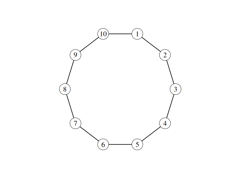
Figure S1: Example ring network with 10 nodes.

The proposed methods are demonstrated for both non-bipartite and bipartite simulation datasets with two time periods $t\in\{0,1\}$. In the non-bipartite setting, consider an unweighted ring network where units are positioned in a circle with each unit having two edges to its two neighbors. See Figure S1 for an example of a ring network with 10 nodes.

In the bipartite network setting, data were simulated using the interference matrix $W^{*}_{2005}$ from the data application where $W^{*}$ (the time subscript is omitted for the remainder of this section since it is not relevant for simulations) represents the potential influence of power plants on counties as derived from an atmospheric transport model in 2005 (see Section 4 for more details). For the simulation, each row of $W^{*}$ is divided by its sum, i.e., $w_{ij}=w_{ij}^{*}/\sum_{j}w_{ij}^{*}$ where $w_{ij}^{*}$ is the $(i,j)$th element of $W^{*}$, so that each row sums to one. The simulation datasets include $2500$ units in the non-bipartite scenario and $3105$ outcome units and $398$ intervention units in the bipartite scenario. The $3105$ outcome units represent counties in the contiguous United States and the $398$ intervention units represent coal power plants.

For both non-bipartite and bipartite networks, observed covariates $X_{j}$, unobserved covariates $U_{j}$, treatments $Z_{j}$, and exposures $G_{i}$ were generated as follows.

$$X_{j}\sim N(0,1),$$

$$U_{j}\sim N(0,1),$$

$$Z_{j}|X_{j},U_{j}\sim\mathrm{Bernoulli}\left(\mathrm{logit}^{-1}(\sin{(x_{j}-2)^{2}}+0.4u_{j})\right),$$

$$G_{i}=\mathbbm{1}\left(\sum_{j}w_{ij}Z_{j}>0.5\right).$$

Note that in the non-bipartite case, $j=i$. In the non-bipartite ring network
$(w_{i,i-3},\dots,w_{i,i},\dots,w_{i,i+3})=(\frac{1}{7},\dots,\frac{1}{7})$ and all other $w_{ij}$ are equal to zero. Thus, the exposure mapping for a unit $i$ equals one if at least four of its closest 6 neighbors and itself had treatment $Z_{j}=1$. In the bipartite network, an exposure of one for an outcome unit $i$ implies that treatments have a large potential influence on that unit.

Outcomes $Y_{it}$ in the non-bipartite network were generated as:

$$Y_{it}=f^{\mathrm{out}}(X_{i-3},\dots,X_{i+3})+u_{i}+G_{i}u_{i}+tf^{\mathrm{out}}(X_{i-3},\dots,X_{i+3})+5t\times G_{i}+\epsilon_{it},$$

where $f^{\mathrm{out}}(X_{i-3},\dots,X_{i+3})=1+0.5\exp(x_{i-3})-2x_{i-2}x_{i-1}+0.1x_{i}^{3}+5\sin{x_{i+1}}-x_{i+2}+10\mathrm{logit}^{-1}(x_{i+3}).$ The simulations consider both the case where the errors $\epsilon_{i}$ are independent and dependent, where the latter implies latent variable dependence. In the independent case, $\epsilon_{it}\sim N(0,1)$ and in the dependent case $\epsilon_{t}=(\epsilon_{1t},\dots,\epsilon_{nt})^{\mathrm{T}}\sim N(0,k^{\mathrm{ring}}(i,j))$ where $k^{\mathrm{ring}}(i,j)=0.6^{d_{ij}}$ and $d_{ij}$ is the path distance between units $i$ and $j$ according to the ring network. The path distance of nodes $(i,j)$ is the smallest number of edges that connect units $i$ and $j$ according to the network. The path distance of a unit with itself is zero.

For the bipartite network, the outcome data generating process was:

$$Y_{it}=f^{\mathrm{out}}(\sum_{j}w_{ij}X_{j})+u_{i}+G_{i}u_{i}+tf^{\mathrm{out}}(\sum_{j}w_{ij}X_{j})+5t\times G_{i}+\epsilon_{it},$$

where $f^{\mathrm{out}}(X_{i}^{*})=3+X_{i}^{*}-2(X_{i}^{*})^{2}+3(X_{i}^{*})^{3},$ with $X_{i}^{*}=\sum_{j}w_{ij}X_{j}$ and $\epsilon_{t}\sim N(0,\Sigma)$ with $\Sigma$ equal to the identity matrix for the independent case. For the dependent error case, the elements of $\Sigma$ have $\sigma^{2}_{i,i^{\prime}}=0.1$ if $d^{\mathrm{out}}(i,i^{\prime})<1.1$ and $\sigma^{2}_{i,i^{\prime}}=0$ otherwise. The distance $d^{\mathrm{out}}(i,i^{\prime})$ is defined as a function of the interference matrix $W$. The interference matrix is a weighted biadjacency matrix that connects intervention units with outcome units. The bipartite graph is projected to an outcome unit graph by defining the following edge weights: $w^{\mathrm{out}}(i,i^{\prime})=\sum_{j}\min(w(i,j),w(i^{\prime},j)).$ The edge weights $w^{\mathrm{out}}(i,i^{\prime})$ connect two outcome units if those two outcome units were both connected to the same intervention unit. Then, distance $d^{\mathrm{out}}(i,i^{\prime})$ was defined to be the weighted shortest path between two units where weights are $1/w^{\mathrm{out}}(i,i^{\prime})$. Intervention units’ covariates and treatments are assumed to be independent and identically distributed so it is not necessary to project the bipartite graph to an intervention unit graph. In both non-bipartite and bipartite settings, the true $\operatorname{AEE}=5$.

For each of the four simulation scenarios, 500 datasets were simulated. Each dataset is evaluated using four different doubly robust estimators. The first three estimators do not use cross-fitting and vary by using parametric, nonparametric, and oracle estimators for the nuisance functions. The estimator with parametric nuisance function estimators employs logistic regression for the treatment propensity score and linear regression for the outcome model. Gaussian process regression with the radial basis kernel was used for the treatment propensity score and Bayesian additive regression trees (BART) was used to model the outcome regression. For the oracle estimators, the true nuisance functions were used. Monte Carlo integration was used in all cases to estimate the exposure propensity score from the estimated treatment propensity scores. The last estimator of the AEE considered was the cross-fit estimator $\hat{\tau}^{\mathrm{DDCF}}$ with nonparametric nuisance function estimators.

The HAC variance estimator $\hat{\sigma}^{2}_{n}$ is used to compute standard errors and create confidence intervals. The uniform kernel is used to give equal weight to all terms $\hat{\phi}_{i}\hat{\phi}_{j}$ if $d(i,j)<b$ where $b$ is the bandwidth parameter. A bandwidth of $b=0$ ignores covariance terms between different units. In the dependent outcome error scenarios, the consequences of ignoring dependence are assessed by setting the bandwidth to zero.

Table 1 provides results from $500$ simulations for each scenario. The estimators with parametric nuisance function estimators performed poorly in all scenarios since the parametric models were mis-specified. In contrast, nonparametric estimation of nuisance functions led to performance on par with using oracle nuisance functions. Cross-fitting did not have a large impact on performance in all scenarios. However, incorrectly setting the bandwidth to zero under the presence of latent outcome dependency yielded poor coverage rates. Overall, nonparametric estimation of nuisance functions led to estimators of the $\operatorname{AEE}$ that had low bias, low mean squared error, and nominal or near nominal coverage rates when dependency was appropriately accounted for.

4 Application

The proposed methods are demonstrated in a real data application to assess the effect of implementing emission control technologies in coal power plants on county-level mortality. In particular, consider as treatments the installation of flue-gas desulfurization scrubbers which reduce SO₂ emissions. Outcomes are county-level deaths per 100,000 due to any circulatory disease, as defined by ICD-10 codes I00-I99. A similar exposure mapping as in the simulations is considered, $G_{it}=\mathbbm{1}(\sum_{j}w_{ijt}Z_{jt}>\alpha)$ where $Z_{jt}=1$ if power plant $j$ installed a scrubber in year $t$ and $Z_{jt}=0$ otherwise. The threshold $\alpha$ and interference weights $w_{ijt}$ are discussed in more detail below.

Interference occurs in this data since county-level mortality by cardiovascular diseases may depend on scrubber installations for coal power plants potentially far away. In this application, the HYSPLIT (Hybrid Single-Particle Lagrangian Integrated Trajectory) model [24, 25] uses an atmospheric model to estimate the movement of air parcels from point sources through three-dimensional space. HyADS (HYSPLIT Average Dispersion) [26] was then used to create a transfer coefficient matrix (TCM) that associates the air parcel densities from power plants to counties. The TCM was calculated for every month and year between January 2002 and December 2007. See Henneman et al. [26] for a characterization of HyADS and the parameter settings used.

Define potential interference burden for a particular county $i$ at time $t$ to be the sum of all power plant air parcel contributions, or $w_{it}=\sum_{j}w_{ijt}$. Counties may vary greatly in their potential interference burden from power plants, and a county with small $w_{it}$ is not necessarily comparable to a county with large $w_{it}$. Under the proposed exposure mapping and with varying potential interference burden, Assumptions 1 and 2 may be violated since $G_{it}=G_{kt}=1$ may not necessarily have the same interpretation for counties $i$ and $k$ that have vastly different potential interference burdens. Additionally, Assumption 4 is violated if $\sum_{j}w_{ijt}<\alpha$ for some $i$ and $t$.

To alleviate this issue, counties are split according to quartiles of potential interference burden. Average $W_{2002},\dots,W_{2007}$ to create the matrix $W^{\mathrm{agg}}$ with elements $w^{\mathrm{agg}}_{ij}=\frac{1}{6}\sum_{t=2002}^{2007}w_{ijt}$. Then, quartiles based on $\sum_{j}w^{\mathrm{agg}}_{ij}Z_{jt}$ can be defined. Within each group, the potential interference burden is normalized to equal 1, i.e., $w_{ijt}^{*}=w_{ijt}/w_{it}$ is used. The smallest two quartiles either have too low potential interference burden (so a measurable exposure effect is not expected) or contain too few counties in the exposed group. Thus, the top two quartiles are analyzed separately. A map showing the potential interference burden groups is shown in Figure 1. The threshold $\alpha$ is defined to be the 75th percentile of the within-quartile $\sum_{j}w_{ijt}Z_{jt}$ for $t=2007$.

The causal estimand corresponds to the effect of having many influential power plants install a scrubber in 2007 on county-level mortality in 2008 among counties with high scrubber exposure. The year 2007 was chosen since many power plants installed scrubbers in this year. Using the notation introduced above, the exposure histories compared are $\bar{g}_{2007}=(0,\dots,0,1)$ and $\bar{g}_{2007}^{\prime}=(0,\dots,0,0)$. Figure 2 shows the counties with high exposure (corresponding to many influential power plants installing a scrubber) in 2007 among the counties with comparable HyADS while Figure 3 shows the number of deaths due to CVDs per 100,000 in each county under study in 2006 and 2008.

Data on coal power plants and atmospheric transport are publicly available from the United States Environmental Protection Agency’s Clean Air Markets Program. County-level mortality data is from CDC WONDER.

Baseline covariates assumed to satisfy the conditional parallel trends assumption are shown in Table 2 and include county-level demographic information from the 2000 Census and power plant-level operating characteristics. At the county-level, power plant covariates are summarized using a weighted average where the weights are from the interference matrix, e.g., $\sum_{j}w_{ij}X_{j}^{\mathrm{int}}$. There were 498 unexposed and 136 exposed counties in the third quartile group according to the exposure mapping defined above. In the fourth quartile group, there were 498 unexposed and 109 exposed counties.

Results are presented using both parametric and nonparametric estimators of the nuisance functions in the DR estimator. In the parametric case, logistic regression was used to model the treatment propensity scores and linear regression to model the outcome trends, both fit using maximum likelihood. In the nonparametric case, logistic Gaussian process regression was used to model the treatment propensity scores and BART to model the outcome trends. In both cases, covariates in the treatment propensity models include power plant level covariates and the covariates of the county where that power plant resides. Similarly, the outcome models include the county-level covariates presented in Table 2. Additionally, 95% confidence intervals are reported using two different bandwidths: $0$ and $1.1$. The bandwidth of $0$ assumes zero covariance between counties while the bandwidth of $1.1$ performed well in the simulations reported above. Results are shown in Table 3. Among counties in the third quartile, the estimated AEE was negative using either parametric or nonparametric nuisance function estimators, but the confidence intervals included zero in all cases. Among counties in the fourth quartile, point estimates were positive, the opposite direction as anticipated since a positive effect implies that more scrubbers installed cause more deaths. However, as in the third quartile, all confidence intervals include zero. These results suggest that the data may be too noisy relative to the size of the true effects and that residual confounding may be present.

5 Discussion

In this paper, semiparametric theory was extended for a doubly robust DiD estimator to the setting with dependent data with possible (bipartite) interference. Under assumptions on the network and interference structure, the DR estimator was shown to be consistent for the AEE and asymptotically normal with variance reaching the semiparametric efficiency bound. Though the network setting was considered in this work, results can be easily extended to the spatial setting by replacing the network topology with a spatial metric space. The estimators were shown to perform well in finite samples through simulations in non-bipartite and bipartite settings. The proposed methods were demonstrated to study the effect of scrubber installations in coal power plants on county-level deaths due to cardiovascular diseases.

Future work may relax some assumptions made in this paper. For instance, networks and the exposure mapping were assumed to be known and non-stochastic but future work may consider modeling the network generation process or different exposure mappings. Additionally, a cross-fitted estimator under a clustered network was proposed that was shown to be CAN. In future work, it may be possible to construct a cross-fit estimator that is CAN for general networks. It is also possible to make stronger assumptions such as clustered networks (implying clustered interference) and compare semiparametric theory in this setting. In general, many of the recent innovations in observational causal inference with interference with an ignorability assumption can be extended to the DiD setting that assumes (conditional) parallel trends.

References

Figures

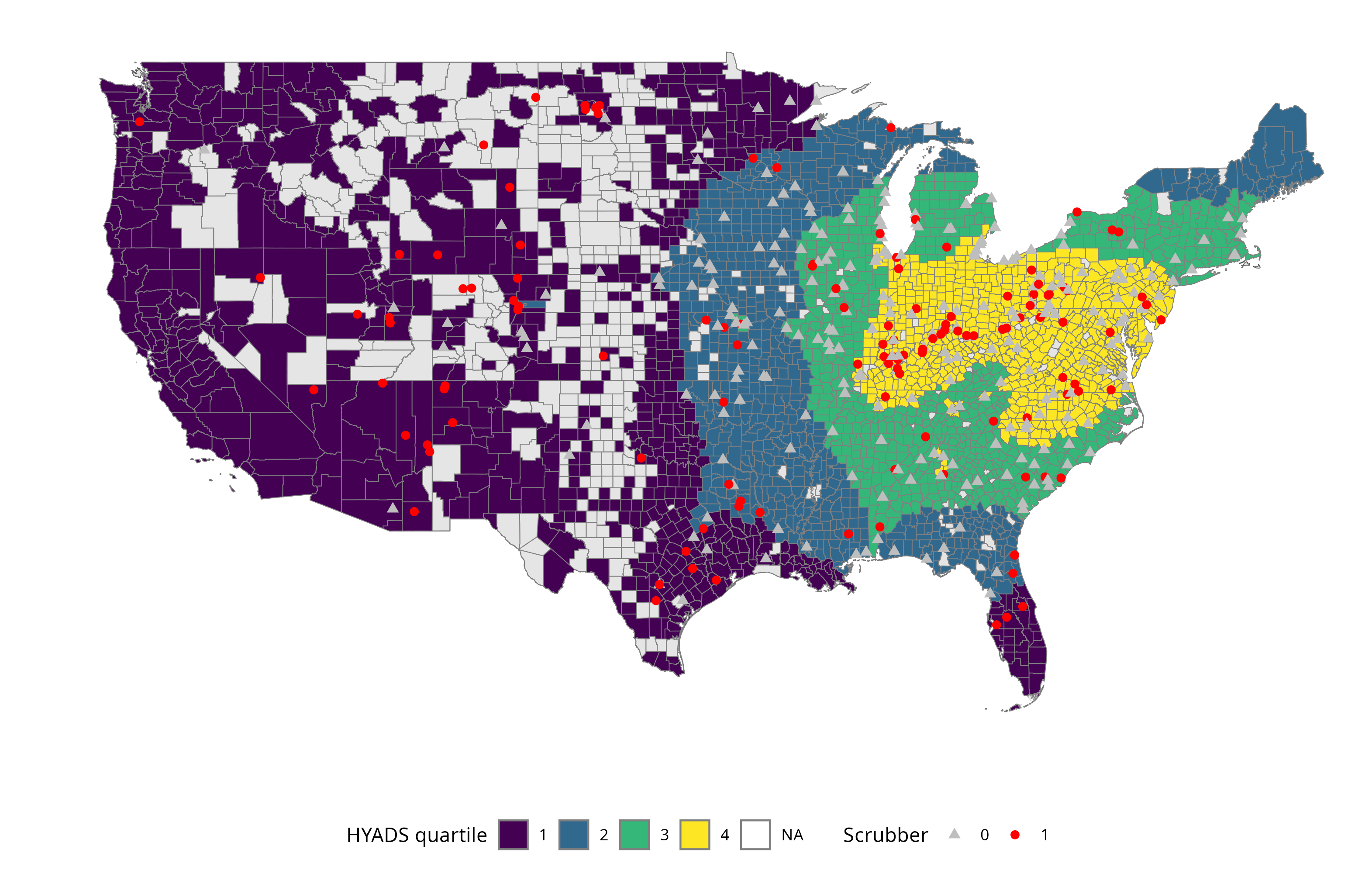
Figure 1: Counties by potential interference quartile and power plants by scrubber status in 2007.

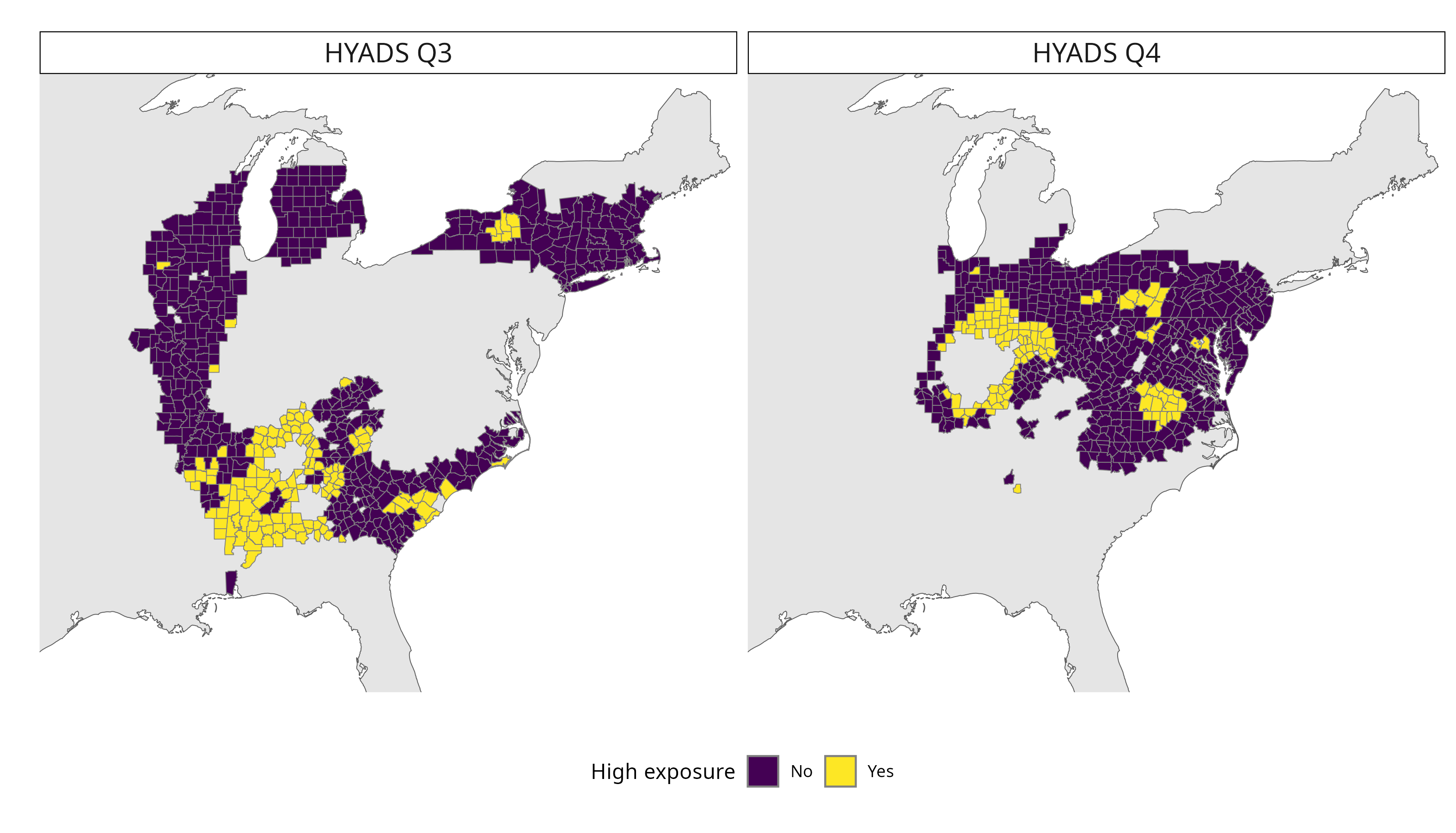
Figure 2: Counties with many influential power plants installing scrubbers in 2007.

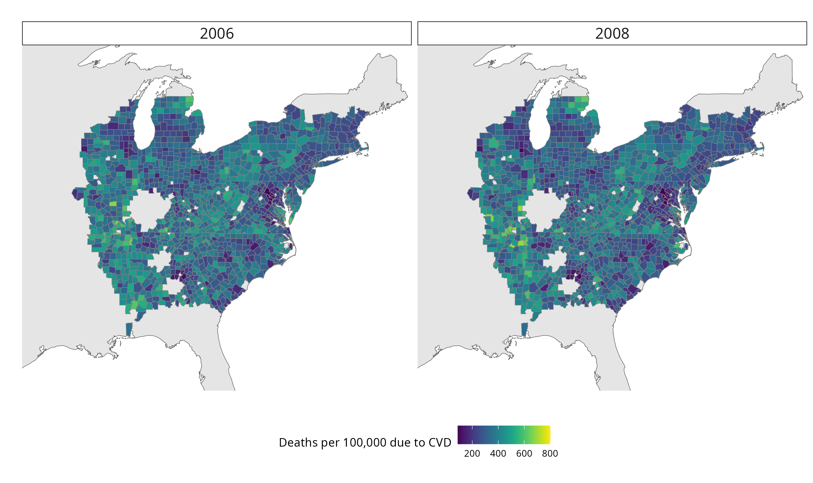
Figure 3: Deaths due to cardiovascular diseases by county and year, per 100,000.

Tables

Table 1: Results from 500 simulations.

Data generation		Estimator parameters			Results
Network	Outcome errors	Band- width	Nuisance function estimators	Cross- fitting	Bias	ESE	ASE	Coverage (%)
Ring	Ind.	0	Parametric	No	0.043	0.115	0.117	93.8
		0	Nonparametric	No	-0.002	0.072	0.070	95.2
		0	Nonparametric	K=5	-0.004	0.078	0.079	96.0
		0	Oracle	NA	-0.004	0.062	0.063	96.0
Ring	Dep.	15	Parametric	No	0.055	0.141	0.133	90.6
		15	Nonparametric	No	0.002	0.107	0.098	93.2
		15	Nonparametric	K=5	0.005	0.109	0.105	95.4
		15	Oracle	NA	0.005	0.100	0.096	94.0
		0	Parametric	No	0.055	0.140	0.117	85.4
		0	Nonparametric	No	-0.001	0.108	0.071	81.0
		0	Nonparametric	K=5	0.004	0.111	0.079	83.8
		0	Oracle	NA	0.006	0.099	0.062	77.8
Bipartite	Ind.	0	Parametric	No	0.009	0.104	0.069	86.8
		0	Nonparametric	No	0.007	0.079	0.071	94.4
		0	Nonparametric	K=15	0.006	0.080	0.073	94.6
		0	Oracle	NA	0.006	0.075	0.070	94.8
Bipartite	Dep.	1.1	Parametric	No	-0.006	0.119	0.092	90.2
		1.1	Nonparametric	No	-0.009	0.100	0.092	95.4
		1.1	Nonparametric	K=15	-0.009	0.099	0.090	94.4
		1.1	Oracle	NA	-0.008	0.095	0.093	96.2
		0	Parametric	No	-0.006	0.119	0.069	78.0
		0	Nonparametric	No	-0.009	0.100	0.072	84.6
		0	Nonparametric	K=15	-0.009	0.099	0.070	83.7
		0	Oracle	NA	-0.008	0.095	0.071	87.2

Ind.: independent, Dep.: dependent, MSE: mean squared error, ASE: average standard error estimates, ESE: empirical standard error, Coverage (%): 95% confidence interval coverage.

Table 2: Summaries of county-level and power plant-level covariates.

Covariate	Mean (SD)
	Quartile 3	Quartile 4
County
Proportion White	0.828 (0.180)	0.873 (0.146)
Proportion Black	0.136 (0.176)	0.096 (0.134)
Proportion Hispanic	0.028 (0.041)	0.022 (0.028)
Proportion female	0.510 (0.015)	0.509 (0.016)
Median age	36.8 (3.0)	37.3 (3.0)
Proportion urban	0.425 (0.293)	0.453 (0.306)
Average household size	2.5 (0.1)	2.5 (0.1)
Proportion in poverty	0.136 (0.064)	0.120 (0.056)
Proportion high school graduate	0.494 (0.065)	0.509 (0.055)
log(Population)	10.8 (1.2)	10.8 (1.2)
log(Population / mi2)	4.6 (1.2)	4.9 (1.3)
Weighted avg. of number of NOx controls	4.2 (0.8)	4.6 (0.4)
Weighted avg. of log(Heat input), mmbtu	17.3 (0.3)	17.3 (0.2)
Weighted avg. of log(Operating time), hours	9.9 (0.2)	9.9 (0.1)
Weighted avg. of prop. with selective non-catalytic reduction	0.1 (0)	0.1 (0.1)
Weighted avg. of participation in ARP Phase II	0.5 (0)	0.5 (0.1)
Power plant
Scrubber	0.314 (0.465)
Number of NOx controls	3 (2.5)
log(Heat input), mmbtu	17.2 (1.2)
log(Operating time), hours	9.6 (0.6)
Proportion with selective non-catalytic reduction	0.108 (0.311)
Participation in ARP Phase II	0.475 (0.500)

ARP: Acid Rain Program, NOx: nitrous oxide.

Table 3: Estimates of the average exposure effect from scrubber installation on number of county-level deaths due to cardiovascular diseases per 100,000.

Nuisance function estimator	Bandwidth	Estimate (95% CI)
		County quartile 3	County quartile 4
Parametric	0	-10.1 (-22.5, 2.3)	12.2 (-0.9, 25.3)
Nonparametric	0	-8.6 (-20.5, 3.4)	9.4 (-3.0, 21.9)
Parametric	1.1	-10.1 (-20.9, 0.7)	12.2 (-0.7, 25.2)
Nonparametric	1.1	-8.6 (-19.2, 2.0)	9.4 (-2.5, 21.4)

6 Supplementary material

6.1 Supplementary figures

6.2 Proof of Proposition 1

The proof of Proposition 1 follows exactly the proof of Theorem 1 in Sant’Anna and Zhou [9] replacing treatment $D$ in Sant’Anna and Zhou with $I(\bar{G}_{t}=\bar{g}_{t})$, $1-D$ with $I(\bar{G}_{t}=\bar{g}_{t}^{\prime})$, and generalizing the time periods from $\{0,1\}$ to $\{t-\delta,t\}$.

6.3 Proof of Proposition 2

Proof of Proposition 2.

Consider the estimator $\operatorname{E}_{n}[\mathbbm{1}(\bar{G}_{t}=\bar{g}_{t})]$ of $\operatorname{P}(\bar{G}_{t}=\bar{g}_{t})$. Under Assumptions 6-8, $\{(\mathbbm{1}(\bar{G}_{t}=\bar{g}_{t}),\frac{\mathbbm{1}(\bar{G}_{t}=\bar{g}_{t}^{\prime})\pi(X;\bar{g}_{t})}{\pi(X;\bar{g}_{t}^{\prime})})^{\mathrm{T}}\}_{i=1}^{n}$ fulfills boundedness, $\psi$-dependence, and sparsity. Then, by Theorem 3.1 of Kojevnikov et al. [17],

$$\operatorname{E}_{n}[\mathbbm{1}(\bar{G}_{t}=\bar{g}_{t})]\rightarrow_{p}\operatorname{E}[\mathbbm{1}(\bar{G}_{t}=\bar{g}_{t})]=\operatorname{P}(\bar{G}_{t}=\bar{g}_{t}).$$

Similarly, by Theorem 3.1 of Kojevnikov et al. [17] and the continuous mapping theorem,

$$\operatorname{E}_{n}\left[\frac{\mathbbm{1}(\bar{G}_{t}=\bar{g}_{t}^{\prime})\hat{\pi}(X;\bar{g}_{t})}{\hat{\pi}(X;\bar{g}_{t}^{\prime})}\right]\rightarrow_{p}\operatorname{E}\left[\frac{\mathbbm{1}(\bar{G}_{t}=\bar{g}_{t}^{\prime})\pi(X;\bar{g}_{t})}{\pi(X;\bar{g}_{t}^{\prime})}\right],$$

since consistency of the exposure propensity score estimators $\hat{\pi}(X;\bar{g}_{t})$ was assumed. Thus, $\hat{h}_{1}(\bar{G})\rightarrow_{p}h_{1}(\bar{G})$ and $\hat{h}_{0}(\bar{G}_{t},X;\hat{\pi})\rightarrow_{p}h_{0}(\bar{G}_{t},X;\pi)$ by the continuous mapping theorem. With another application of the continuous mapping theorem,

$$\hat{\tau}^{\mathrm{DR}}\rightarrow_{p}\tau^{\mathrm{DR}}.$$

Finally, by Proposition 1, $\hat{\tau}^{\mathrm{DR}}\rightarrow_{p}\tau$. ∎

6.4 Proof of Theorem 1

The doubly-robust plug-in estimator is re-stated below.

$$\hat{\tau}^{\mathrm{DR}} :=\mathbb{P}_{n}\left[\left(\frac{\mathbbm{1}(\bar{G}_{t}=\bar{g}_{t})}{\mathbb{P}_{n}[\mathbbm{1}(\bar{G}_{t}=\bar{g}_{t})]}-\frac{\mathbbm{1}(\bar{G}_{t}=\bar{g}_{t}^{\prime})\hat{\pi}(X;\bar{g}_{t})}{\hat{\pi}(X;\bar{g}_{t}^{\prime})\mathbb{P}_{n}[\frac{\mathbbm{1}(\bar{G}_{t}=\bar{g}_{t}^{\prime})\hat{\pi}(X;\bar{g}_{t})}{\hat{\pi}(X;\bar{g}_{t}^{\prime})}]}\right)\left(\Delta Y-\hat{\mu}_{g^{\prime},\delta}(X)\right)\right].$$

With some re-arranging and noticing that $\mathbb{P}_{n}\{\frac{\mathbbm{1}(\bar{G}_{t}=\bar{g}_{t})}{\mathbb{P}_{n}\{\mathbbm{1}(\bar{G}_{t}=\bar{g}_{t})\}}\tau\}=\tau$, it can be seen that $\hat{\tau}^{\mathrm{DR}}$ is a solution to the estimating equation

$$\mathbb{P}_{n}\phi_{i}=0.$$

The proof follows the strategy outlined by Kennedy (2023) [27]. Let $\mathcal{P}$ be a statistical model that contains the observed data distribution $\mathbb{P}$, i.e., $\mathbb{P}\in\mathcal{P}$. Let $\Psi(\mathbb{P})$ be the estimand of interest, corresponding to $\tau^{\mathrm{DR}}$ to emphasize that the target parameter is a function of the observed data distribution. Similarly, let $\Psi(\hat{\mathbb{P}})$ be the plug-in estimator of that estimand, corresponding to $\hat{\tau}^{\mathrm{DR}}$ where $\hat{\mathbb{P}})$ is the data distribution imposed by using plug-in estimators of the nuisance functions. Further, let $\mathbb{P}_{n}$ denote the empirical measure in the sense that $\mathbb{P}_{n}(f(Q))=n^{-1}\sum_{i=1}^{n}f(Q_{i})$ for some function $f$ and data $Q$. Similarly $\mathbb{P}(\cdot)$ denotes the expectation in the sense of $\mathbb{P}(f(Q))=\int f(q)d\mathbb{P}(q)$ for the (potentially random) function $f$. Then, by the von Mises expansion of $\Psi(\hat{\mathbb{P}})$ about $\Psi(\mathbb{P})$,

$$\Psi(\hat{\mathbb{P}})-\Psi(\mathbb{P}) =\int\phi(\hat{\mathbb{P}})d(\hat{\mathbb{P}}-\mathbb{P})+R_{2}(\hat{\mathbb{P}},\mathbb{P})$$

$$=-\mathbb{P}\{\phi(\hat{\mathbb{P}})\}+R_{2}(\hat{\mathbb{P}},\mathbb{P}),$$

$$=(\mathbb{P}_{n}-\mathbb{P})(\phi(\hat{\mathbb{P}}))-(\mathbb{P}_{n}-\mathbb{P})(\phi(\mathbb{P}))+(\mathbb{P}_{n}-\mathbb{P})(\phi(\mathbb{P}))+R_{2}(\hat{\mathbb{P}},\mathbb{P})$$

$$=(\mathbb{P}_{n}-\mathbb{P})(\phi(\hat{\mathbb{P}})-\phi(\mathbb{P}))+(\mathbb{P}_{n}-\mathbb{P})(\phi(\mathbb{P}))+R_{2}(\hat{\mathbb{P}},\mathbb{P}),$$

where $\phi(\mathbb{P})$ is the EIF and $\phi(\hat{\mathbb{P}})$ is the plug-in EIF estimator with $\mathbb{P}_{n}(\phi(\hat{\mathbb{P}}))=0$. The root-$n$ scaled second term converges to $N(0,\mathrm{Var}(\phi(\mathbb{P}))$ by the central limit theorem (Theorem 3.2) from Kojevnikov et al. [17] and Assumptions 6-8. Below it is shown that the first term (empirical process term) and the third term (remainder term) go to zero at the root-$n$ rate.

For the remainder of the proof the function arguments are dropped for notational simplicity when the context is clear, e.g., $\pi_{g}$ in place of $\pi(X;\bar{g}_{t})$. The DR superscript from $\tau$ and $\hat{\tau}$ is also dropped. First, the remainder term is shown to converge to zero.

$$R_{2}(\hat{\mathbb{P}},\mathbb{P}) =\Psi(\hat{\mathbb{P}})+\int\phi(\hat{\mathbb{P}})d\mathbb{P}-\Psi(\mathbb{P})$$

$$=\hat{\tau}+\int\left[(\hat{h}_{1}-\hat{h}_{0})(\Delta Y-\hat{\mu}_{g^{\prime},\delta}(X))-\hat{h}_{1}\hat{\tau}\right]d\mathbb{P}-\tau$$

$$=\hat{\tau}-\frac{\hat{\tau}}{\mathbb{P}_{n}(\mathbbm{1}(\bar{G}_{t}=\bar{g}_{t}))}\int\mathbbm{1}(\bar{G}_{t}=\bar{g}_{t})d\mathbb{P}+\int\left[(\hat{h}_{1}-\hat{h}_{0})(\Delta Y-\hat{\mu}_{g^{\prime},\delta}(X))\right]d\mathbb{P}-\tau$$

$$=\hat{\tau}\left(1-\frac{\mathbb{P}(\mathbbm{1}(\bar{G}_{t}=\bar{g}_{t}))}{\mathbb{P}_{n}(\mathbbm{1}(\bar{G}_{t}=\bar{g}_{t}))}\right)+\int\left[(\hat{h}_{1}-\hat{h}_{0})(\Delta Y-\hat{\mu}_{g^{\prime},\delta}(X))\right]d\mathbb{P}-\tau$$

$$=\hat{\tau}\left(1-\frac{\mathbb{P}(\mathbbm{1}(\bar{G}_{t}=\bar{g}_{t}))}{\mathbb{P}_{n}(\mathbbm{1}(\bar{G}_{t}=\bar{g}_{t}))}\right)+\int\left[(\hat{h}_{1}-\hat{h}_{0})(\Delta Y-\hat{\mu}_{g^{\prime},\delta}(X))-(h_{1}-h_{0})(\Delta Y-\mu_{g^{\prime},\delta}(X))\right]d\mathbb{P}$$

$$=\hat{\tau}\left(1-\frac{\mathbb{P}(\mathbbm{1}(\bar{G}_{t}=\bar{g}_{t}))}{\mathbb{P}_{n}(\mathbbm{1}(\bar{G}_{t}=\bar{g}_{t}))}\right)$$

$$\hskip 20.00003pt+\int\left[(\hat{h}_{1}-h_{1})\Delta Y-(\hat{h}_{0}-h_{0})\Delta Y-(\hat{h}_{1}-\hat{h}_{0})\hat{\mu}_{g^{\prime},\delta}+(h_{1}-h_{0})\mu_{g^{\prime},\delta}\right]d\mathbb{P}$$

$$=\hat{\tau}\left(1-\frac{\mathbb{P}(\mathbbm{1}(\bar{G}_{t}=\bar{g}_{t}))}{\mathbb{P}_{n}(\mathbbm{1}(\bar{G}_{t}=\bar{g}_{t}))}\right)$$

$$\hskip 20.00003pt+\int\left[(\hat{h}_{1}-h_{1})\Delta Y-(\hat{h}_{0}-h_{0})\Delta Y+(h_{1}\mu_{g^{\prime},\delta}-\hat{h}_{1}\hat{\mu}_{g^{\prime},\delta})-(h_{0}\mu_{g^{\prime},\delta}-\hat{h}_{0}\hat{\mu}_{g^{\prime},\delta})\right]d\mathbb{P}.$$

Recall that $h_{1}=\frac{\mathbbm{1}(\bar{G}_{t}=\bar{g}_{t})}{\operatorname{E}[\mathbbm{1}(\bar{G}_{t}=\bar{g}_{t})]}$ and $h_{0}=\frac{\mathbbm{1}(\bar{G}_{t}=\bar{g}_{t}^{\prime}){\pi}(x;\bar{g}_{t})}{{\pi}(x;\bar{g}_{t}^{\prime})\mathrm{E}[(\mathbbm{1}(\bar{G}_{t}=\bar{g}_{t}^{\prime}){\pi}(x;\bar{g}_{t})/{\pi}(x;\bar{g}_{t}^{\prime})]}$. Also note that $\mathrm{E}[(\mathbbm{1}(\bar{G}_{t}=\bar{g}_{t}^{\prime}){\pi}(x;\bar{g}_{t})/{\pi}(x;\bar{g}_{t}^{\prime})]=\operatorname{E}[\mathbbm{1}(\bar{G}_{t}=\bar{g}_{t})]$ so $h_{0}=\frac{\mathbbm{1}(\bar{G}_{t}=\bar{g}_{t}^{\prime}){\pi}(x;\bar{g}_{t})}{{\pi}(x;\bar{g}_{t}^{\prime})\mathrm{E}[\mathbbm{1}(\bar{G}_{t}=\bar{g}_{t})]}$. Also let $\hat{h}_{1}$ and $\hat{h}_{0}$ denote plug-in estimators of $h_{1}$ and $h_{0}$, respectively, where the expectations in the denominators are estimated with the empirical measure $\operatorname{E}_{n}$. Now, each term in the integral is analyzed separately.

$$(\hat{h}_{1}-h_{1})\Delta Y =\left[\frac{\mathbbm{1}(\bar{G}_{t}=\bar{g}_{t})}{\mathbb{P}_{n}[\mathbbm{1}(\bar{G}_{t}=\bar{g}_{t})]}-\frac{\mathbbm{1}(\bar{G}_{t}=\bar{g}_{t})}{\operatorname{E}[\mathbbm{1}(\bar{G}_{t}=\bar{g}_{t})]}\right]\Delta Y$$

$$=\left[\frac{\mathbbm{1}(\bar{G}_{t}=\bar{g}_{t})[\mathbb{P}(\mathbbm{1}(\bar{G}_{t}=\bar{g}_{t}))-\mathbb{P}_{n}(\mathbbm{1}(\bar{G}_{t}=\bar{g}_{t}))]}{\mathbb{P}_{n}(\mathbbm{1}(\bar{G}_{t}=\bar{g}_{t}))\mathbb{P}(\mathbbm{1}(\bar{G}_{t}=\bar{g}_{t}))}\right]\Delta Y.$$

$$(\hat{h}_{0}-h_{0})\Delta Y =\left[\frac{\mathbbm{1}(\bar{G}_{t}=\bar{g}_{t}^{\prime})\hat{\pi}(X;\bar{g}_{t})}{\hat{\pi}(X;\bar{g}_{t}^{\prime})\mathbb{P}_{n}[\frac{\mathbbm{1}(\bar{G}_{t}=\bar{g}_{t}^{\prime})\hat{\pi}(X;\bar{g}_{t})}{\hat{\pi}(X;\bar{g}_{t}^{\prime})}]}-\frac{\mathbbm{1}(\bar{G}_{t}=\bar{g}_{t}^{\prime}){\pi}(x;\bar{g}_{t})}{{\pi}(x;\bar{g}_{t}^{\prime})\mathrm{E}[\mathbbm{1}(\bar{G}_{t}=\bar{g}_{t})]}\right]\Delta Y$$

$$=\bigg{[}\frac{\mathbbm{1}(\bar{G}_{t}=\bar{g}_{t}^{\prime})\hat{\pi}(X;\bar{g}_{t})}{\hat{\pi}(X;\bar{g}_{t}^{\prime})\mathbb{P}_{n}[\mathbbm{1}(\bar{G}_{t}=\bar{g}_{t})]}-\frac{\mathbbm{1}(\bar{G}_{t}=\bar{g}_{t}^{\prime})\hat{\pi}_{g}[\mathbb{P}(\mathbbm{1}(\bar{G}_{t}=\bar{g}_{t}))-\mathbb{P}_{n}(\mathbbm{1}(\bar{G}_{t}=\bar{g}_{t}))]}{\hat{\pi}_{g^{\prime}}\mathbb{P}(\mathbbm{1}(\bar{G}_{t}=\bar{g}_{t}))\mathbb{P}_{n}(\mathbbm{1}(\bar{G}_{t}=\bar{g}_{t}))}$$

$$\hskip 20.00003pt+\frac{\mathbbm{1}(\bar{G}_{t}=\bar{g}_{t}^{\prime})\hat{\pi}_{g}[\mathbb{P}(\mathbbm{1}(\bar{G}_{t}=\bar{g}_{t}))-\mathbb{P}_{n}(\mathbbm{1}(\bar{G}_{t}=\bar{g}_{t}))]}{\hat{\pi}_{g^{\prime}}\mathbb{P}(\mathbbm{1}(\bar{G}_{t}=\bar{g}_{t}))\mathbb{P}_{n}(\mathbbm{1}(\bar{G}_{t}=\bar{g}_{t}))}$$

$$\hskip 20.00003pt-\frac{\mathbbm{1}(\bar{G}_{t}=\bar{g}_{t}^{\prime}){\pi}(x;\bar{g}_{t})}{{\pi}(x;\bar{g}_{t}^{\prime})\mathrm{E}[\mathbbm{1}(\bar{G}_{t}=\bar{g}_{t})]}\bigg{]}\Delta Y$$

$$=\left[\frac{\mathbbm{1}(\bar{G}_{t}=\bar{g}_{t}^{\prime})\hat{\pi}_{g}}{\hat{\pi}_{g^{\prime}}\mathbb{P}(\mathbbm{1}(\bar{G}_{t}=\bar{g}_{t}))}-\frac{\mathbbm{1}(\bar{G}_{t}=\bar{g}_{t}^{\prime}){\pi}(x;\bar{g}_{t})}{{\pi}(x;\bar{g}_{t}^{\prime})\mathrm{E}[\mathbbm{1}(\bar{G}_{t}=\bar{g}_{t})]}\right]\Delta Y$$

$$\hskip 20.00003pt+\frac{\mathbbm{1}(\bar{G}_{t}=\bar{g}_{t}^{\prime})\hat{\pi}_{g}[\mathbb{P}(\mathbbm{1}(\bar{G}_{t}=\bar{g}_{t}))-\mathbb{P}_{n}(\mathbbm{1}(\bar{G}_{t}=\bar{g}_{t}))]}{\hat{\pi}_{g^{\prime}}\mathbb{P}(\mathbbm{1}(\bar{G}_{t}=\bar{g}_{t}))\mathbb{P}_{n}(\mathbbm{1}(\bar{G}_{t}=\bar{g}_{t}))}\Delta Y.$$

Simplifying the first term of the first product above,

$$\frac{\mathbbm{1}(\bar{G}_{t}=\bar{g}_{t}^{\prime})\hat{\pi}_{g}}{\hat{\pi}_{g^{\prime}}\mathbb{P}(\mathbbm{1}(\bar{G}_{t}=\bar{g}_{t}))}-\frac{\mathbbm{1}(\bar{G}_{t}=\bar{g}_{t}^{\prime}){\pi}(x;\bar{g}_{t})}{{\pi}(x;\bar{g}_{t}^{\prime})\mathrm{E}[\mathbbm{1}(\bar{G}_{t}=\bar{g}_{t})]} =\frac{\mathbbm{1}(\bar{G}_{t}=\bar{g}_{t}^{\prime})\hat{\pi}_{g}}{\hat{\pi}_{g^{\prime}}\mathbb{P}(\mathbbm{1}(\bar{G}_{t}=\bar{g}_{t}))}-\frac{\mathbbm{1}(\bar{G}_{t}=\bar{g}_{t}^{\prime})\hat{\pi}_{g}[\pi_{g^{\prime}}-\hat{\pi}_{g^{\prime}}]}{\pi_{g^{\prime}}\hat{\pi}_{g^{\prime}}\mathbb{P}(\mathbbm{1}(\bar{G}_{t}=\bar{g}_{t}))}$$

$$\hskip 20.00003pt+\frac{\mathbbm{1}(\bar{G}_{t}=\bar{g}_{t}^{\prime})\hat{\pi}_{g}[\pi_{g^{\prime}}-\hat{\pi}_{g^{\prime}}]}{\pi_{g^{\prime}}\hat{\pi}_{g^{\prime}}\mathbb{P}(\mathbbm{1}(\bar{G}_{t}=\bar{g}_{t}))}-\frac{\mathbbm{1}(\bar{G}_{t}=\bar{g}_{t}^{\prime}){\pi}(x;\bar{g}_{t})}{{\pi}(x;\bar{g}_{t}^{\prime})\mathrm{E}[\mathbbm{1}(\bar{G}_{t}=\bar{g}_{t})]}$$

$$=\frac{\mathbbm{1}(\bar{G}_{t}=\bar{g}_{t}^{\prime})\hat{\pi}_{g}}{\pi_{g^{\prime}}\mathbb{P}(\mathbbm{1}(\bar{G}_{t}=\bar{g}_{t}))}-\frac{\mathbbm{1}(\bar{G}_{t}=\bar{g}_{t}^{\prime}){\pi}(x;\bar{g}_{t})}{{\pi}(x;\bar{g}_{t}^{\prime})\mathrm{E}[\mathbbm{1}(\bar{G}_{t}=\bar{g}_{t})]}$$

$$\hskip 20.00003pt+\frac{\mathbbm{1}(\bar{G}_{t}=\bar{g}_{t}^{\prime})\hat{\pi}_{g}[\pi_{g^{\prime}}-\hat{\pi}_{g^{\prime}}]}{\pi_{g^{\prime}}\hat{\pi}_{g^{\prime}}\mathbb{P}(\mathbbm{1}(\bar{G}_{t}=\bar{g}_{t}))}$$

$$=\frac{\mathbbm{1}(\bar{G}_{t}=\bar{g}_{t}^{\prime})}{\pi_{g^{\prime}}\mathbb{P}(\mathbbm{1}(\bar{G}_{t}=\bar{g}_{t}))}[\hat{\pi}_{g}-\pi_{g}]+\frac{\mathbbm{1}(\bar{G}_{t}=\bar{g}_{t}^{\prime})\hat{\pi}_{g}[\pi_{g^{\prime}}-\hat{\pi}_{g^{\prime}}]}{\pi_{g^{\prime}}\hat{\pi}_{g^{\prime}}\mathbb{P}(\mathbbm{1}(\bar{G}_{t}=\bar{g}_{t}))}.$$

$$h_{1}\mu_{g^{\prime},\delta}-\hat{h}_{1}\hat{\mu}_{g^{\prime},\delta} =\frac{\mathbbm{1}(\bar{G}_{t}=\bar{g}_{t})}{\operatorname{E}[\mathbbm{1}(\bar{G}_{t}=\bar{g}_{t})]}\mu_{g^{\prime},\delta}-\frac{\mathbbm{1}(\bar{G}_{t}=\bar{g}_{t})}{\mathbb{P}_{n}[\mathbbm{1}(\bar{G}_{t}=\bar{g}_{t})]}\hat{\mu}_{g^{\prime},\delta}$$

$$=\frac{\mathbbm{1}(\bar{G}_{t}=\bar{g}_{t})}{\operatorname{E}[\mathbbm{1}(\bar{G}_{t}=\bar{g}_{t})]}\mu_{g^{\prime},\delta}-\frac{\mathbbm{1}(\bar{G}_{t}=\bar{g}_{t})}{\mathbb{P}_{n}[\mathbbm{1}(\bar{G}_{t}=\bar{g}_{t})]}\hat{\mu}_{g^{\prime},\delta}$$

$$\hskip 20.00003pt+\frac{\mathbbm{1}(\bar{G}_{t}=\bar{g}_{t})\hat{\mu}_{g^{\prime},\delta}[\mathbb{P}(\mathbbm{1}(\bar{G}_{t}=\bar{g}_{t}))-\mathbb{P}_{n}(\mathbbm{1}(\bar{G}_{t}=\bar{g}_{t}))]}{\mathbb{P}_{n}(\mathbbm{1}(\bar{G}_{t}=\bar{g}_{t}))\mathbb{P}(\mathbbm{1}(\bar{G}_{t}=\bar{g}_{t}))}$$

$$\hskip 20.00003pt-\frac{\mathbbm{1}(\bar{G}_{t}=\bar{g}_{t})\hat{\mu}_{g^{\prime},\delta}[\mathbb{P}(\mathbbm{1}(\bar{G}_{t}=\bar{g}_{t}))-\mathbb{P}_{n}(\mathbbm{1}(\bar{G}_{t}=\bar{g}_{t}))]}{\mathbb{P}_{n}(\mathbbm{1}(\bar{G}_{t}=\bar{g}_{t}))\mathbb{P}(\mathbbm{1}(\bar{G}_{t}=\bar{g}_{t}))}$$

$$=\frac{\mathbbm{1}(\bar{G}_{t}=\bar{g}_{t})}{\operatorname{E}[\mathbbm{1}(\bar{G}_{t}=\bar{g}_{t})]}\mu_{g^{\prime},\delta}-\frac{\mathbbm{1}(\bar{G}_{t}=\bar{g}_{t})}{\mathbb{P}(\mathbbm{1}(\bar{G}_{t}=\bar{g}_{t}))}\hat{\mu}_{g^{\prime},\delta}$$

$$\hskip 20.00003pt-\frac{\mathbbm{1}(\bar{G}_{t}=\bar{g}_{t})\hat{\mu}_{g^{\prime},\delta}[\mathbb{P}(\mathbbm{1}(\bar{G}_{t}=\bar{g}_{t}))-\mathbb{P}_{n}(\mathbbm{1}(\bar{G}_{t}=\bar{g}_{t}))]}{\mathbb{P}_{n}(\mathbbm{1}(\bar{G}_{t}=\bar{g}_{t}))\mathbb{P}(\mathbbm{1}(\bar{G}_{t}=\bar{g}_{t}))}$$

$$=\frac{\mathbbm{1}(\bar{G}_{t}=\bar{g}_{t})}{\operatorname{E}[\mathbbm{1}(\bar{G}_{t}=\bar{g}_{t})]}[\mu_{g^{\prime},\delta}-\hat{\mu}_{g^{\prime},\delta}]-\frac{\mathbbm{1}(\bar{G}_{t}=\bar{g}_{t})\hat{\mu}_{g^{\prime},\delta}[\mathbb{P}(\mathbbm{1}(\bar{G}_{t}=\bar{g}_{t}))-\mathbb{P}_{n}(\mathbbm{1}(\bar{G}_{t}=\bar{g}_{t}))]}{\mathbb{P}_{n}(\mathbbm{1}(\bar{G}_{t}=\bar{g}_{t}))\mathbb{P}(\mathbbm{1}(\bar{G}_{t}=\bar{g}_{t}))}.$$

$$h_{0}\mu_{g^{\prime},\delta}-\hat{h}_{0}\hat{\mu}_{g^{\prime},\delta} =\frac{\mathbbm{1}(\bar{G}_{t}=\bar{g}_{t}^{\prime}){\pi}(x;\bar{g}_{t})}{{\pi}(x;\bar{g}_{t}^{\prime})\mathrm{E}[\mathbbm{1}(\bar{G}_{t}=\bar{g}_{t})]}\mu_{g^{\prime},\delta}-\frac{\mathbbm{1}(\bar{G}_{t}=\bar{g}_{t}^{\prime})\hat{\pi}(X;\bar{g}_{t})}{\hat{\pi}(X;\bar{g}_{t}^{\prime})\mathbb{P}_{n}[\mathbbm{1}(\bar{G}_{t}=\bar{g}_{t})]}\hat{\mu}_{g^{\prime},\delta}$$

$$=\frac{\mathbbm{1}(\bar{G}_{t}=\bar{g}_{t}^{\prime}){\pi}(x;\bar{g}_{t})}{{\pi}(x;\bar{g}_{t}^{\prime})\mathrm{E}[\mathbbm{1}(\bar{G}_{t}=\bar{g}_{t})]}\mu_{g^{\prime},\delta}-\frac{\mathbbm{1}(\bar{G}_{t}=\bar{g}_{t}^{\prime})\hat{\pi}(X;\bar{g}_{t})}{\hat{\pi}(X;\bar{g}_{t}^{\prime})\mathbb{P}_{n}[\mathbbm{1}(\bar{G}_{t}=\bar{g}_{t})]}\hat{\mu}_{g^{\prime},\delta}$$

$$\hskip 20.00003pt+\frac{\mathbbm{1}(\bar{G}_{t}=\bar{g}_{t}^{\prime})\hat{\pi}_{g}[\mathbb{P}(\mathbbm{1}(\bar{G}_{t}=\bar{g}_{t}))-\mathbb{P}_{n}(\mathbbm{1}(\bar{G}_{t}=\bar{g}_{t}))]}{\hat{\pi}_{g^{\prime}}\mathbb{P}(\mathbbm{1}(\bar{G}_{t}=\bar{g}_{t}))\mathbb{P}_{n}(\mathbbm{1}(\bar{G}_{t}=\bar{g}_{t}))}\hat{\mu}_{g^{\prime},\delta}$$

$$\hskip 20.00003pt-\frac{\mathbbm{1}(\bar{G}_{t}=\bar{g}_{t}^{\prime})\hat{\pi}_{g}[\mathbb{P}(\mathbbm{1}(\bar{G}_{t}=\bar{g}_{t}))-\mathbb{P}_{n}(\mathbbm{1}(\bar{G}_{t}=\bar{g}_{t}))]}{\hat{\pi}_{g^{\prime}}\mathbb{P}(\mathbbm{1}(\bar{G}_{t}=\bar{g}_{t}))\mathbb{P}_{n}(\mathbbm{1}(\bar{G}_{t}=\bar{g}_{t}))}\hat{\mu}_{g^{\prime},\delta}$$

$$=\frac{\mathbbm{1}(\bar{G}_{t}=\bar{g}_{t}^{\prime}){\pi}(x;\bar{g}_{t})}{{\pi}(x;\bar{g}_{t}^{\prime})\mathrm{E}[\mathbbm{1}(\bar{G}_{t}=\bar{g}_{t})]}\mu_{g^{\prime},\delta}-\frac{\mathbbm{1}(\bar{G}_{t}=\bar{g}_{t}^{\prime})\hat{\pi}_{g}}{\hat{\pi}_{g^{\prime}}\mathbb{P}(\mathbbm{1}(\bar{G}_{t}=\bar{g}_{t}))}\hat{\mu}_{g^{\prime},\delta}$$

$$\hskip 20.00003pt-\frac{\mathbbm{1}(\bar{G}_{t}=\bar{g}_{t}^{\prime})\hat{\pi}_{g}[\mathbb{P}(\mathbbm{1}(\bar{G}_{t}=\bar{g}_{t}))-\mathbb{P}_{n}(\mathbbm{1}(\bar{G}_{t}=\bar{g}_{t}))]}{\hat{\pi}_{g^{\prime}}\mathbb{P}(\mathbbm{1}(\bar{G}_{t}=\bar{g}_{t}))\mathbb{P}_{n}(\mathbbm{1}(\bar{G}_{t}=\bar{g}_{t}))}\hat{\mu}_{g^{\prime},\delta}$$

$$=\frac{\mathbbm{1}(\bar{G}_{t}=\bar{g}_{t}^{\prime}){\pi}(x;\bar{g}_{t})}{{\pi}(x;\bar{g}_{t}^{\prime})\mathrm{E}[\mathbbm{1}(\bar{G}_{t}=\bar{g}_{t})]}\mu_{g^{\prime},\delta}-\frac{\mathbbm{1}(\bar{G}_{t}=\bar{g}_{t}^{\prime})\hat{\pi}_{g}}{\hat{\pi}_{g^{\prime}}\mathbb{P}(\mathbbm{1}(\bar{G}_{t}=\bar{g}_{t}))}\hat{\mu}_{g^{\prime},\delta}$$

$$\hskip 20.00003pt+\frac{\mathbbm{1}(\bar{G}_{t}=\bar{g}_{t}^{\prime})\hat{\pi}_{g}\hat{\mu}_{g^{\prime},\delta}[\pi_{g^{\prime}}-\hat{\pi}_{g^{\prime}}]}{\hat{\pi}_{g^{\prime}}\pi_{g^{\prime}}\mathbb{P}(\mathbbm{1}(\bar{G}_{t}=\bar{g}_{t}))}-\frac{\mathbbm{1}(\bar{G}_{t}=\bar{g}_{t}^{\prime})\hat{\pi}_{g}\hat{\mu}_{g^{\prime},\delta}[\pi_{g^{\prime}}-\hat{\pi}_{g^{\prime}}]}{\hat{\pi}_{g^{\prime}}\pi_{g^{\prime}}\mathbb{P}(\mathbbm{1}(\bar{G}_{t}=\bar{g}_{t}))}$$

$$\hskip 20.00003pt-\frac{\mathbbm{1}(\bar{G}_{t}=\bar{g}_{t}^{\prime})\hat{\pi}_{g}[\mathbb{P}(\mathbbm{1}(\bar{G}_{t}=\bar{g}_{t}))-\mathbb{P}_{n}(\mathbbm{1}(\bar{G}_{t}=\bar{g}_{t}))]}{\hat{\pi}_{g^{\prime}}\mathbb{P}(\mathbbm{1}(\bar{G}_{t}=\bar{g}_{t}))\mathbb{P}_{n}(\mathbbm{1}(\bar{G}_{t}=\bar{g}_{t}))}\hat{\mu}_{g^{\prime},\delta}$$

$$=\frac{\mathbbm{1}(\bar{G}_{t}=\bar{g}_{t}^{\prime}){\pi}(x;\bar{g}_{t})}{{\pi}(x;\bar{g}_{t}^{\prime})\mathrm{E}[\mathbbm{1}(\bar{G}_{t}=\bar{g}_{t})]}\mu_{g^{\prime},\delta}-\frac{\mathbbm{1}(\bar{G}_{t}=\bar{g}_{t}^{\prime})\hat{\pi}_{g}}{\pi_{g^{\prime}}\mathbb{P}(\mathbbm{1}(\bar{G}_{t}=\bar{g}_{t}))}\hat{\mu}_{g^{\prime},\delta}-\frac{\mathbbm{1}(\bar{G}_{t}=\bar{g}_{t}^{\prime})\hat{\pi}_{g}\hat{\mu}_{g^{\prime},\delta}[\pi_{g^{\prime}}-\hat{\pi}_{g^{\prime}}]}{\hat{\pi}_{g^{\prime}}\pi_{g^{\prime}}\mathbb{P}(\mathbbm{1}(\bar{G}_{t}=\bar{g}_{t}))}$$

$$\hskip 20.00003pt-\frac{\mathbbm{1}(\bar{G}_{t}=\bar{g}_{t}^{\prime})\hat{\pi}_{g}[\mathbb{P}(\mathbbm{1}(\bar{G}_{t}=\bar{g}_{t}))-\mathbb{P}_{n}(\mathbbm{1}(\bar{G}_{t}=\bar{g}_{t}))]}{\hat{\pi}_{g^{\prime}}\mathbb{P}(\mathbbm{1}(\bar{G}_{t}=\bar{g}_{t}))\mathbb{P}_{n}(\mathbbm{1}(\bar{G}_{t}=\bar{g}_{t}))}\hat{\mu}_{g^{\prime},\delta}$$

$$=\frac{\mathbbm{1}(\bar{G}_{t}=\bar{g}_{t}^{\prime})}{\pi_{g^{\prime}}\mathbb{P}(\mathbbm{1}(\bar{G}_{t}=\bar{g}_{t}))}[\pi_{g}\mu_{g^{\prime},\delta}-\hat{\pi}_{g}\hat{\mu}_{g^{\prime},\delta}]-\frac{\mathbbm{1}(\bar{G}_{t}=\bar{g}_{t}^{\prime})\hat{\pi}_{g}\hat{\mu}_{g^{\prime},\delta}[\pi_{g^{\prime}}-\hat{\pi}_{g^{\prime}}]}{\hat{\pi}_{g^{\prime}}\pi_{g^{\prime}}\mathbb{P}(\mathbbm{1}(\bar{G}_{t}=\bar{g}_{t}))}$$

$$\hskip 20.00003pt-\frac{\mathbbm{1}(\bar{G}_{t}=\bar{g}_{t}^{\prime})\hat{\pi}_{g}[\mathbb{P}(\mathbbm{1}(\bar{G}_{t}=\bar{g}_{t}))-\mathbb{P}_{n}(\mathbbm{1}(\bar{G}_{t}=\bar{g}_{t}))]}{\hat{\pi}_{g^{\prime}}\mathbb{P}(\mathbbm{1}(\bar{G}_{t}=\bar{g}_{t}))\mathbb{P}_{n}(\mathbbm{1}(\bar{G}_{t}=\bar{g}_{t}))}\hat{\mu}_{g^{\prime},\delta}$$

$$=\frac{\mathbbm{1}(\bar{G}_{t}=\bar{g}_{t}^{\prime})}{\pi_{g^{\prime}}\mathbb{P}(\mathbbm{1}(\bar{G}_{t}=\bar{g}_{t}))}[\pi_{g}\mu_{g^{\prime},\delta}-\pi_{g}\hat{\mu}_{g^{\prime},\delta}+\pi_{g}\hat{\mu}_{g^{\prime},\delta}-\hat{\pi}_{g}\hat{\mu}_{g^{\prime},\delta}]-\frac{\mathbbm{1}(\bar{G}_{t}=\bar{g}_{t}^{\prime})\hat{\pi}_{g}\hat{\mu}_{g^{\prime},\delta}[\pi_{g^{\prime}}-\hat{\pi}_{g^{\prime}}]}{\hat{\pi}_{g^{\prime}}\pi_{g^{\prime}}\mathbb{P}(\mathbbm{1}(\bar{G}_{t}=\bar{g}_{t}))}$$

$$\hskip 20.00003pt-\frac{\mathbbm{1}(\bar{G}_{t}=\bar{g}_{t}^{\prime})\hat{\pi}_{g}[\mathbb{P}(\mathbbm{1}(\bar{G}_{t}=\bar{g}_{t}))-\mathbb{P}_{n}(\mathbbm{1}(\bar{G}_{t}=\bar{g}_{t}))]}{\hat{\pi}_{g^{\prime}}\mathbb{P}(\mathbbm{1}(\bar{G}_{t}=\bar{g}_{t}))\mathbb{P}_{n}(\mathbbm{1}(\bar{G}_{t}=\bar{g}_{t}))}\hat{\mu}_{g^{\prime},\delta}$$

$$=\frac{\mathbbm{1}(\bar{G}_{t}=\bar{g}_{t}^{\prime})}{\pi_{g^{\prime}}\mathbb{P}(\mathbbm{1}(\bar{G}_{t}=\bar{g}_{t}))}[\pi_{g}(\mu_{g^{\prime},\delta}-\hat{\mu}_{g^{\prime},\delta})+\hat{\mu}_{g^{\prime},\delta}(\pi_{g}-\hat{\pi}_{g})-\mu_{g^{\prime},\delta}(\pi_{g}-\hat{\pi}_{g})+\mu_{g^{\prime},\delta}(\pi_{g}-\hat{\pi}_{g})]$$

$$\hskip 20.00003pt-\frac{\mathbbm{1}(\bar{G}_{t}=\bar{g}_{t}^{\prime})\hat{\pi}_{g}\hat{\mu}_{g^{\prime},\delta}[\pi_{g^{\prime}}-\hat{\pi}_{g^{\prime}}]}{\hat{\pi}_{g^{\prime}}\pi_{g^{\prime}}\mathbb{P}(\mathbbm{1}(\bar{G}_{t}=\bar{g}_{t}))}$$

$$\hskip 20.00003pt-\frac{\mathbbm{1}(\bar{G}_{t}=\bar{g}_{t}^{\prime})\hat{\pi}_{g}[\mathbb{P}(\mathbbm{1}(\bar{G}_{t}=\bar{g}_{t}))-\mathbb{P}_{n}(\mathbbm{1}(\bar{G}_{t}=\bar{g}_{t}))]}{\hat{\pi}_{g^{\prime}}\mathbb{P}(\mathbbm{1}(\bar{G}_{t}=\bar{g}_{t}))\mathbb{P}_{n}(\mathbbm{1}(\bar{G}_{t}=\bar{g}_{t}))}\hat{\mu}_{g^{\prime},\delta}$$

$$=\frac{\mathbbm{1}(\bar{G}_{t}=\bar{g}_{t}^{\prime})}{\pi_{g^{\prime}}\mathbb{P}(\mathbbm{1}(\bar{G}_{t}=\bar{g}_{t}))}[\pi_{g}(\mu_{g^{\prime},\delta}-\hat{\mu}_{g^{\prime},\delta})+(\hat{\mu}_{g^{\prime},\delta}-\mu_{g^{\prime},\delta})(\pi_{g}-\hat{\pi}_{g})+\mu_{g^{\prime},\delta}(\pi_{g}-\hat{\pi}_{g})]$$

$$\hskip 20.00003pt-\frac{\mathbbm{1}(\bar{G}_{t}=\bar{g}_{t}^{\prime})\hat{\pi}_{g}\hat{\mu}_{g^{\prime},\delta}[\pi_{g^{\prime}}-\hat{\pi}_{g^{\prime}}]}{\hat{\pi}_{g^{\prime}}\pi_{g^{\prime}}\mathbb{P}(\mathbbm{1}(\bar{G}_{t}=\bar{g}_{t}))}$$

$$\hskip 20.00003pt-\frac{\mathbbm{1}(\bar{G}_{t}=\bar{g}_{t}^{\prime})\hat{\pi}_{g}[\mathbb{P}(\mathbbm{1}(\bar{G}_{t}=\bar{g}_{t}))-\mathbb{P}_{n}(\mathbbm{1}(\bar{G}_{t}=\bar{g}_{t}))]}{\hat{\pi}_{g^{\prime}}\mathbb{P}(\mathbbm{1}(\bar{G}_{t}=\bar{g}_{t}))\mathbb{P}_{n}(\mathbbm{1}(\bar{G}_{t}=\bar{g}_{t}))}\hat{\mu}_{g^{\prime},\delta}.$$

Now, the remainder term can be written as:

$$R_{2}(\hat{\mathbb{P}},\mathbb{P}) =\hat{\tau}\left(1-\frac{\mathbb{P}(\mathbbm{1}(\bar{G}_{t}=\bar{g}_{t}))}{\mathbb{P}_{n}(\mathbbm{1}(\bar{G}_{t}=\bar{g}_{t}))}\right)$$

$$\hskip 20.00003pt+\int\bigg{\{}\left[\frac{\mathbbm{1}(\bar{G}_{t}=\bar{g}_{t})[\mathbb{P}(\mathbbm{1}(\bar{G}_{t}=\bar{g}_{t}))-\mathbb{P}_{n}(\mathbbm{1}(\bar{G}_{t}=\bar{g}_{t}))]}{\mathbb{P}_{n}(\mathbbm{1}(\bar{G}_{t}=\bar{g}_{t}))\mathbb{P}(\mathbbm{1}(\bar{G}_{t}=\bar{g}_{t}))}\right]\Delta Y$$

$$\hskip 20.00003pt-\left[\frac{\mathbbm{1}(\bar{G}_{t}=\bar{g}_{t}^{\prime})}{\pi_{g^{\prime}}\mathbb{P}(\mathbbm{1}(\bar{G}_{t}=\bar{g}_{t}))}[\hat{\pi}_{g}-\pi_{g}]+\frac{\mathbbm{1}(\bar{G}_{t}=\bar{g}_{t}^{\prime})\hat{\pi}_{g}[\pi_{g^{\prime}}-\hat{\pi}_{g^{\prime}}]}{\pi_{g^{\prime}}\hat{\pi}_{g^{\prime}}\mathbb{P}(\mathbbm{1}(\bar{G}_{t}=\bar{g}_{t}))}\right]\Delta Y$$

$$\hskip 20.00003pt-\frac{\mathbbm{1}(\bar{G}_{t}=\bar{g}_{t}^{\prime})\hat{\pi}_{g}[\mathbb{P}(\mathbbm{1}(\bar{G}_{t}=\bar{g}_{t}))-\mathbb{P}_{n}(\mathbbm{1}(\bar{G}_{t}=\bar{g}_{t}))]}{\hat{\pi}_{g^{\prime}}\mathbb{P}(\mathbbm{1}(\bar{G}_{t}=\bar{g}_{t}))\mathbb{P}_{n}(\mathbbm{1}(\bar{G}_{t}=\bar{g}_{t}))}\Delta Y$$

$$\hskip 20.00003pt+\frac{\mathbbm{1}(\bar{G}_{t}=\bar{g}_{t})}{\operatorname{E}[\mathbbm{1}(\bar{G}_{t}=\bar{g}_{t})]}[\mu_{g^{\prime},\delta}-\hat{\mu}_{g^{\prime},\delta}]-\frac{\mathbbm{1}(\bar{G}_{t}=\bar{g}_{t})\hat{\mu}_{g^{\prime},\delta}[\mathbb{P}(\mathbbm{1}(\bar{G}_{t}=\bar{g}_{t}))-\mathbb{P}_{n}(\mathbbm{1}(\bar{G}_{t}=\bar{g}_{t}))]}{\mathbb{P}_{n}(\mathbbm{1}(\bar{G}_{t}=\bar{g}_{t}))\mathbb{P}(\mathbbm{1}(\bar{G}_{t}=\bar{g}_{t}))}$$

$$\hskip 20.00003pt-\frac{\mathbbm{1}(\bar{G}_{t}=\bar{g}_{t}^{\prime})}{\pi_{g^{\prime}}\mathbb{P}(\mathbbm{1}(\bar{G}_{t}=\bar{g}_{t}))}[\pi_{g}(\mu_{g^{\prime},\delta}-\hat{\mu}_{g^{\prime},\delta})+(\hat{\mu}_{g^{\prime},\delta}-\mu_{g^{\prime},\delta})(\pi_{g}-\hat{\pi}_{g})+\mu_{g^{\prime},\delta}(\pi_{g}-\hat{\pi}_{g})]$$

$$\hskip 20.00003pt+\frac{\mathbbm{1}(\bar{G}_{t}=\bar{g}_{t}^{\prime})\hat{\pi}_{g}\hat{\mu}_{g^{\prime},\delta}[\pi_{g^{\prime}}-\hat{\pi}_{g^{\prime}}]}{\hat{\pi}_{g^{\prime}}\pi_{g^{\prime}}\mathbb{P}(\mathbbm{1}(\bar{G}_{t}=\bar{g}_{t}))}+\frac{\mathbbm{1}(\bar{G}_{t}=\bar{g}_{t}^{\prime})\hat{\pi}_{g}[\mathbb{P}(\mathbbm{1}(\bar{G}_{t}=\bar{g}_{t}))-\mathbb{P}_{n}(\mathbbm{1}(\bar{G}_{t}=\bar{g}_{t}))]}{\hat{\pi}_{g^{\prime}}\mathbb{P}(\mathbbm{1}(\bar{G}_{t}=\bar{g}_{t}))\mathbb{P}_{n}(\mathbbm{1}(\bar{G}_{t}=\bar{g}_{t}))}\hat{\mu}_{g^{\prime},\delta}\bigg{\}}d\mathbb{P}$$

$$=\hat{\tau}\left(1-\frac{\mathbb{P}(\mathbbm{1}(\bar{G}_{t}=\bar{g}_{t}))}{\mathbb{P}_{n}(\mathbbm{1}(\bar{G}_{t}=\bar{g}_{t}))}\right)$$

$$\hskip 20.00003pt-\operatorname{E}\left[\frac{\mathbbm{1}(\bar{G}_{t}=\bar{g}_{t}^{\prime})[\hat{\pi}_{g}-\pi_{g}]}{\pi_{g^{\prime}}\mathbb{P}(\mathbbm{1}(\bar{G}_{t}=\bar{g}_{t}))}\Delta Y\right]+\operatorname{E}\left[\frac{\mathbbm{1}(\bar{G}_{t}=\bar{g}_{t}^{\prime})}{\pi_{g^{\prime}}\mathbb{P}(\mathbbm{1}(\bar{G}_{t}=\bar{g}_{t}))}\mu_{g^{\prime},\delta}(\hat{\pi}_{g}-\pi_{g})\right]$$

$$\hskip 20.00003pt+\int\left\{-\frac{\mathbbm{1}(\bar{G}_{t}=\bar{g}_{t}^{\prime})}{\pi_{g^{\prime}}\mathbb{P}(\mathbbm{1}(\bar{G}_{t}=\bar{g}_{t}))}[(\hat{\mu}_{g^{\prime},\delta}-\mu_{g^{\prime},\delta})(\pi_{g}-\hat{\pi}_{g})]\right\}d\mathbb{P}$$

$$\hskip 20.00003pt-\operatorname{E}\left[\frac{\mathbbm{1}(\bar{G}_{t}=\bar{g}_{t}^{\prime})\hat{\pi}_{g}[\pi_{g^{\prime}}-\hat{\pi}_{g^{\prime}}]}{\pi_{g^{\prime}}\hat{\pi}_{g^{\prime}}\mathbb{P}(\mathbbm{1}(\bar{G}_{t}=\bar{g}_{t}))}\Delta Y\right]+\operatorname{E}\left[\frac{\mathbbm{1}(\bar{G}_{t}=\bar{g}_{t}^{\prime})\hat{\pi}_{g}\hat{\mu}_{g^{\prime},\delta}[\pi_{g^{\prime}}-\hat{\pi}_{g^{\prime}}]}{\hat{\pi}_{g^{\prime}}\pi_{g^{\prime}}\mathbb{P}(\mathbbm{1}(\bar{G}_{t}=\bar{g}_{t}))}\right]$$

$$\hskip 20.00003pt+\operatorname{E}\left[\frac{\mathbbm{1}(\bar{G}_{t}=\bar{g}_{t})}{\mathbb{P}(\mathbbm{1}(\bar{G}_{t}=\bar{g}_{t})}[\mu_{g^{\prime},\delta}-\hat{\mu}_{g^{\prime},\delta}]\right]-\operatorname{E}\left[\frac{\mathbbm{1}(\bar{G}_{t}=\bar{g}_{t}^{\prime})}{\pi_{g^{\prime}}\mathbb{P}(\mathbbm{1}(\bar{G}_{t}=\bar{g}_{t}))}\pi_{g}(\mu_{g^{\prime},\delta}-\hat{\mu}_{g^{\prime},\delta})\right]$$

$$\hskip 20.00003pt+\int\bigg{\{}\left[\frac{\mathbbm{1}(\bar{G}_{t}=\bar{g}_{t})[\mathbb{P}(\mathbbm{1}(\bar{G}_{t}=\bar{g}_{t}))-\mathbb{P}_{n}(\mathbbm{1}(\bar{G}_{t}=\bar{g}_{t}))]}{\mathbb{P}_{n}(\mathbbm{1}(\bar{G}_{t}=\bar{g}_{t}))\mathbb{P}(\mathbbm{1}(\bar{G}_{t}=\bar{g}_{t}))}\right]\Delta Y$$

$$\hskip 20.00003pt-\frac{\mathbbm{1}(\bar{G}_{t}=\bar{g}_{t}^{\prime})\hat{\pi}_{g}[\mathbb{P}(\mathbbm{1}(\bar{G}_{t}=\bar{g}_{t}))-\mathbb{P}_{n}(\mathbbm{1}(\bar{G}_{t}=\bar{g}_{t}))]}{\hat{\pi}_{g^{\prime}}\mathbb{P}(\mathbbm{1}(\bar{G}_{t}=\bar{g}_{t}))\mathbb{P}_{n}(\mathbbm{1}(\bar{G}_{t}=\bar{g}_{t}))}\Delta Y$$

$$\hskip 20.00003pt-\frac{\mathbbm{1}(\bar{G}_{t}=\bar{g}_{t})\hat{\mu}_{g^{\prime},\delta}[\mathbb{P}(\mathbbm{1}(\bar{G}_{t}=\bar{g}_{t}))-\mathbb{P}_{n}(\mathbbm{1}(\bar{G}_{t}=\bar{g}_{t}))]}{\mathbb{P}_{n}(\mathbbm{1}(\bar{G}_{t}=\bar{g}_{t}))\mathbb{P}(\mathbbm{1}(\bar{G}_{t}=\bar{g}_{t}))}$$

$$\hskip 20.00003pt+\frac{\mathbbm{1}(\bar{G}_{t}=\bar{g}_{t}^{\prime})\hat{\pi}_{g}[\mathbb{P}(\mathbbm{1}(\bar{G}_{t}=\bar{g}_{t}))-\mathbb{P}_{n}(\mathbbm{1}(\bar{G}_{t}=\bar{g}_{t}))]}{\hat{\pi}_{g^{\prime}}\mathbb{P}(\mathbbm{1}(\bar{G}_{t}=\bar{g}_{t}))\mathbb{P}_{n}(\mathbbm{1}(\bar{G}_{t}=\bar{g}_{t}))}\hat{\mu}_{g^{\prime},\delta}\bigg{\}}d\mathbb{P}$$

$$=\hat{\tau}\left(1-\frac{\mathbb{P}(\mathbbm{1}(\bar{G}_{t}=\bar{g}_{t}))}{\mathbb{P}_{n}(\mathbbm{1}(\bar{G}_{t}=\bar{g}_{t}))}\right)$$

$$\hskip 20.00003pt+\operatorname{E}\left[\frac{\hat{\pi}_{g}}{\hat{\pi}_{g^{\prime}}\mathbb{P}(\mathbbm{1}(\bar{G}_{t}=\bar{g}_{t}))}(\pi_{g^{\prime}}-\hat{\pi}_{g^{\prime}})(\hat{\mu}_{g^{\prime}}-\mu_{g^{\prime}})\right]$$

$$\hskip 20.00003pt+\frac{1}{\mathbb{P}(\mathbbm{1}(\bar{G}_{t}=\bar{g}_{t}))}\frac{\mathbb{P}(\mathbbm{1}(\bar{G}_{t}=\bar{g}_{t}))-\mathbb{P}_{n}(\mathbbm{1}(\bar{G}_{t}=\bar{g}_{t}))}{\mathbb{P}_{n}(\mathbbm{1}(\bar{G}_{t}=\bar{g}_{t}))}$$

$$\hskip 20.00003pt\times\operatorname{E}\left[\mathbbm{1}(\bar{G}_{t}=\bar{g}_{t})\Delta Y-\frac{\mathbbm{1}(\bar{G}_{t}=\bar{g}_{t}^{\prime})\hat{\pi}_{g}\Delta Y}{\hat{\pi}_{g^{\prime}}}-\mathbbm{1}(\bar{G}_{t}=\bar{g}_{t})\hat{\mu}_{g^{\prime},\delta}+\frac{\mathbbm{1}(\bar{G}_{t}=\bar{g}_{t}^{\prime})\hat{\pi}_{g}\hat{\mu}_{g^{\prime},\delta}}{\hat{\pi}_{g^{\prime}}}\right],$$

where the result that $\operatorname{E}[\mathbbm{1}(\bar{G}_{t}=\bar{g}_{t})\Delta Y]=\operatorname{E}[\operatorname{E}[\mathbbm{1}(\bar{G}_{t}=\bar{g}_{t})\Delta Y|X]]=\operatorname{E}[\mu_{g}\pi_{g}]$ is used. Continuing, the remainder term is equal to:

$$R_{2}(\hat{\mathbb{P}},\mathbb{P})=\hat{\tau}\left(1-\frac{\mathbb{P}(\mathbbm{1}(\bar{G}_{t}=\bar{g}_{t}))}{\mathbb{P}_{n}(\mathbbm{1}(\bar{G}_{t}=\bar{g}_{t}))}\right)$$

$$\hskip 20.00003pt+\operatorname{E}\left[\frac{\hat{\pi}_{g}}{\hat{\pi}_{g^{\prime}}\mathbb{P}(\mathbbm{1}(\bar{G}_{t}=\bar{g}_{t}))}(\pi_{g^{\prime}}-\hat{\pi}_{g^{\prime}})(\hat{\mu}_{g^{\prime}}-\mu_{g^{\prime}})\right]+\operatorname{E}\left[\frac{1}{\mathbb{P}(\mathbbm{1}(\bar{G}_{t}=\bar{g}_{t}))}(\hat{\mu}_{g^{\prime}}-\mu_{g^{\prime}})(\hat{\pi}_{g}-\pi_{g})\right]$$

$$\hskip 20.00003pt+\frac{1}{\mathbb{P}(\mathbbm{1}(\bar{G}_{t}=\bar{g}_{t}))}\frac{\mathbb{P}(\mathbbm{1}(\bar{G}_{t}=\bar{g}_{t}))-\mathbb{P}_{n}(\mathbbm{1}(\bar{G}_{t}=\bar{g}_{t}))}{\mathbb{P}_{n}(\mathbbm{1}(\bar{G}_{t}=\bar{g}_{t}))}$$

$$\hskip 20.00003pt\times\operatorname{E}\left[\mu_{g}\pi_{g}-\frac{\pi_{g^{\prime}}\hat{\pi}_{g}\mu_{g^{\prime}}}{\hat{\pi}_{g^{\prime}}}-\pi_{g}\hat{\mu}_{g^{\prime},\delta}+\frac{\pi_{g}\hat{\pi}_{g}\hat{\mu}_{g^{\prime},\delta}}{\hat{\pi}_{g^{\prime}}}\right]$$

$$=\hat{\tau}\left(1-\frac{\mathbb{P}(\mathbbm{1}(\bar{G}_{t}=\bar{g}_{t}))}{\mathbb{P}_{n}(\mathbbm{1}(\bar{G}_{t}=\bar{g}_{t}))}\right)$$

$$\hskip 20.00003pt+\operatorname{E}\left[\frac{\hat{\pi}_{g}}{\hat{\pi}_{g^{\prime}}\mathbb{P}(\mathbbm{1}(\bar{G}_{t}=\bar{g}_{t}))}(\pi_{g^{\prime}}-\hat{\pi}_{g^{\prime}})(\hat{\mu}_{g^{\prime}}-\mu_{g^{\prime}})\right]+\operatorname{E}\left[\frac{1}{\mathbb{P}(\mathbbm{1}(\bar{G}_{t}=\bar{g}_{t}))}(\hat{\mu}_{g^{\prime}}-\mu_{g^{\prime}})(\hat{\pi}_{g}-\pi_{g})\right]$$

$$\hskip 20.00003pt+\frac{1}{\mathbb{P}(\mathbbm{1}(\bar{G}_{t}=\bar{g}_{t}))}\frac{\mathbb{P}(\mathbbm{1}(\bar{G}_{t}=\bar{g}_{t}))-\mathbb{P}_{n}(\mathbbm{1}(\bar{G}_{t}=\bar{g}_{t}))}{\mathbb{P}_{n}(\mathbbm{1}(\bar{G}_{t}=\bar{g}_{t}))}$$

$$\hskip 20.00003pt\times\operatorname{E}\left[\mu_{g}\pi_{g}-\mu_{g^{\prime}}\pi_{g}+\mu_{g^{\prime}}\pi_{g}-\frac{\pi_{g^{\prime}}\hat{\pi}_{g}\mu_{g^{\prime}}}{\hat{\pi}_{g^{\prime}}}-\pi_{g}\hat{\mu}_{g^{\prime},\delta}+\frac{\pi_{g}\hat{\pi}_{g}\hat{\mu}_{g^{\prime},\delta}}{\hat{\pi}_{g^{\prime}}}\right]$$

$$=\hat{\tau}\left(1-\frac{\mathbb{P}(\mathbbm{1}(\bar{G}_{t}=\bar{g}_{t}))}{\mathbb{P}_{n}(\mathbbm{1}(\bar{G}_{t}=\bar{g}_{t}))}\right)$$

$$\hskip 20.00003pt+\operatorname{E}\left[\frac{\hat{\pi}_{g}}{\hat{\pi}_{g^{\prime}}\mathbb{P}(\mathbbm{1}(\bar{G}_{t}=\bar{g}_{t})}(\pi_{g^{\prime}}-\hat{\pi}_{g^{\prime}})(\hat{\mu}_{g^{\prime}}-\mu_{g^{\prime}})\right]+\operatorname{E}\left[\frac{1}{\mathbb{P}(\mathbbm{1}(\bar{G}_{t}=\bar{g}_{t}))}(\hat{\mu}_{g^{\prime}}-\mu_{g^{\prime}})(\hat{\pi}_{g}-\pi_{g})\right]$$

$$\hskip 20.00003pt+\frac{\mathbb{P}(\mathbbm{1}(\bar{G}_{t}=\bar{g}_{t}))-\mathbb{P}_{n}(\mathbbm{1}(\bar{G}_{t}=\bar{g}_{t}))}{\mathbb{P}_{n}(\mathbbm{1}(\bar{G}_{t}=\bar{g}_{t}))}\left\{\tau+\frac{1}{\mathbb{P}(\mathbbm{1}(\bar{G}_{t}=\bar{g}_{t}))}\operatorname{E}\left[\mu_{g^{\prime}}\pi_{g}-\frac{\pi_{g^{\prime}}\hat{\pi}_{g}\mu_{g^{\prime}}}{\hat{\pi}_{g^{\prime}}}-\pi_{g}\hat{\mu}_{g^{\prime},\delta}+\frac{\pi_{g}\hat{\pi}_{g}\hat{\mu}_{g^{\prime},\delta}}{\hat{\pi}_{g^{\prime}}}\right]\right\}$$

$$=(\hat{\tau}-\tau)\frac{\mathbb{P}_{n}(\mathbbm{1}(\bar{G}_{t}=\bar{g}_{t}))-\mathbb{P}(\mathbbm{1}(\bar{G}_{t}=\bar{g}_{t}))}{\mathbb{P}_{n}(\mathbbm{1}(\bar{G}_{t}=\bar{g}_{t}))}$$

$$\hskip 20.00003pt+\operatorname{E}\left[\frac{\hat{\pi}_{g}}{\hat{\pi}_{g^{\prime}}\mathbb{P}(\mathbbm{1}(\bar{G}_{t}=\bar{g}_{t})}(\pi_{g^{\prime}}-\hat{\pi}_{g^{\prime}})(\hat{\mu}_{g^{\prime}}-\mu_{g^{\prime}})\right]+\operatorname{E}\left[\frac{1}{\mathbb{P}(\mathbbm{1}(\bar{G}_{t}=\bar{g}_{t}))}(\hat{\mu}_{g^{\prime}}-\mu_{g^{\prime}})(\hat{\pi}_{g}-\pi_{g})\right]$$

$$\hskip 20.00003pt+\frac{\mathbb{P}(\mathbbm{1}(\bar{G}_{t}=\bar{g}_{t}))-\mathbb{P}_{n}(\mathbbm{1}(\bar{G}_{t}=\bar{g}_{t}))}{\mathbb{P}_{n}(\mathbbm{1}(\bar{G}_{t}=\bar{g}_{t}))}\frac{1}{\mathbb{P}(\mathbbm{1}(\bar{G}_{t}=\bar{g}_{t}))}\operatorname{E}\left[\pi_{g}(\mu_{g^{\prime},\delta}-\hat{\mu}_{g^{\prime},\delta})-\frac{\pi_{g^{\prime}}\hat{\pi}_{g}}{\hat{\pi}_{g^{\prime}}}(\mu_{g^{\prime},\delta}-\hat{\mu}_{g^{\prime},\delta})\right]$$

$$=(\hat{\tau}-\tau)\frac{\mathbb{P}_{n}(\mathbbm{1}(\bar{G}_{t}=\bar{g}_{t}))-\mathbb{P}(\mathbbm{1}(\bar{G}_{t}=\bar{g}_{t}))}{\mathbb{P}_{n}(\mathbbm{1}(\bar{G}_{t}=\bar{g}_{t}))}$$

$$\hskip 20.00003pt+\operatorname{E}\left[\frac{\hat{\pi}_{g}}{\hat{\pi}_{g^{\prime}}\mathbb{P}(\mathbbm{1}(\bar{G}_{t}=\bar{g}_{t})}(\pi_{g^{\prime}}-\hat{\pi}_{g^{\prime}})(\hat{\mu}_{g^{\prime}}-\mu_{g^{\prime}})\right]+\operatorname{E}\left[\frac{1}{\mathbb{P}(\mathbbm{1}(\bar{G}_{t}=\bar{g}_{t}))}(\hat{\mu}_{g^{\prime}}-\mu_{g^{\prime}})(\hat{\pi}_{g}-\pi_{g})\right]$$

$$\hskip 20.00003pt+\frac{\mathbb{P}(\mathbbm{1}(\bar{G}_{t}=\bar{g}_{t}))-\mathbb{P}_{n}(\mathbbm{1}(\bar{G}_{t}=\bar{g}_{t}))}{\mathbb{P}_{n}(\mathbbm{1}(\bar{G}_{t}=\bar{g}_{t}))}\frac{1}{\mathbb{P}(\mathbbm{1}(\bar{G}_{t}=\bar{g}_{t}))}\operatorname{E}\left[(\hat{\mu}_{g^{\prime},\delta}-\mu_{g^{\prime},\delta})\left(\frac{\pi_{g^{\prime}}\hat{\pi}_{g}}{\hat{\pi}_{g^{\prime}}}-\pi_{g}\right)\right]$$

$$=(\hat{\tau}-\tau)\frac{\mathbb{P}_{n}(\mathbbm{1}(\bar{G}_{t}=\bar{g}_{t}))-\mathbb{P}(\mathbbm{1}(\bar{G}_{t}=\bar{g}_{t}))}{\mathbb{P}_{n}(\mathbbm{1}(\bar{G}_{t}=\bar{g}_{t}))}$$

$$\hskip 20.00003pt+\operatorname{E}\left[\frac{\hat{\pi}_{g}}{\hat{\pi}_{g^{\prime}}\mathbb{P}(\mathbbm{1}(\bar{G}_{t}=\bar{g}_{t}))}(\pi_{g^{\prime}}-\hat{\pi}_{g^{\prime}})(\hat{\mu}_{g^{\prime}}-\mu_{g^{\prime}})\right]+\operatorname{E}\left[\frac{1}{\mathbb{P}(\mathbbm{1}(\bar{G}_{t}=\bar{g}_{t}))}(\hat{\mu}_{g^{\prime}}-\mu_{g^{\prime}})(\hat{\pi}_{g}-\pi_{g})\right]$$

$$\hskip 20.00003pt+\frac{\mathbb{P}(\mathbbm{1}(\bar{G}_{t}=\bar{g}_{t}))-\mathbb{P}_{n}(\mathbbm{1}(\bar{G}_{t}=\bar{g}_{t}))}{\mathbb{P}_{n}(\mathbbm{1}(\bar{G}_{t}=\bar{g}_{t}))}\frac{1}{\mathbb{P}(\mathbbm{1}(\bar{G}_{t}=\bar{g}_{t}))}\operatorname{E}\left[(\hat{\mu}_{g^{\prime},\delta}-\mu_{g^{\prime},\delta})\left(\hat{\pi}_{g}-\pi_{g}+\frac{\hat{\pi}_{g}(\pi_{g^{\prime}}-\hat{\pi}_{g^{\prime}})}{\hat{\pi}_{g^{\prime}}}\right)\right]$$

$$=(\hat{\tau}-\tau)\frac{\mathbb{P}_{n}(\mathbbm{1}(\bar{G}_{t}=\bar{g}_{t}))-\mathbb{P}(\mathbbm{1}(\bar{G}_{t}=\bar{g}_{t}))}{\mathbb{P}_{n}(\mathbbm{1}(\bar{G}_{t}=\bar{g}_{t}))}$$

$$\hskip 20.00003pt+\left(1+\frac{\mathbb{P}(\mathbbm{1}(\bar{G}_{t}=\bar{g}_{t}))-\mathbb{P}_{n}(\mathbbm{1}(\bar{G}_{t}=\bar{g}_{t}))}{\mathbb{P}_{n}(\mathbbm{1}(\bar{G}_{t}=\bar{g}_{t}))}\right)\frac{1}{\mathbb{P}(\mathbbm{1}(\bar{G}_{t}=\bar{g}_{t}))}\operatorname{E}\left[(\hat{\mu}_{g^{\prime},\delta}-\mu_{g^{\prime},\delta})(\hat{\pi}_{g}-\pi_{g})\right]$$

$$\hskip 20.00003pt-\left(1+\frac{\mathbb{P}(\mathbbm{1}(\bar{G}_{t}=\bar{g}_{t}))-\mathbb{P}_{n}(\mathbbm{1}(\bar{G}_{t}=\bar{g}_{t}))}{\mathbb{P}_{n}(\mathbbm{1}(\bar{G}_{t}=\bar{g}_{t}))}\right)\operatorname{E}\left[\frac{\hat{\pi}_{g}}{\hat{\pi}_{g^{\prime}}\mathbb{P}(\mathbbm{1}(\bar{G}_{t}=\bar{g}_{t}))}(\hat{\pi}_{g^{\prime}}-\pi_{g^{\prime}})(\hat{\mu}_{g^{\prime}}-\mu_{g^{\prime}})\right],$$

Thus, $\sqrt{n}R_{2}(\hat{\mathbb{P}},\mathbb{P})=o_{\mathbb{P}}(1)$ using the dependent data central limit theorem and law of large numbers from above and if $\|\hat{\pi}_{g^{\prime}}-\pi_{g^{\prime}}\|\|\hat{\mu}_{g^{\prime}}-\mu_{g^{\prime}}\|=o_{\mathbb{P}}(n^{-1/2})$. To see this, note that $\hat{\tau}-\tau=o_{\mathbb{P}}(1)$ by consistency result above and $\sqrt{n}(\mathbb{P}_{n}-\mathbb{P})(\mathbbm{1}(\bar{G}_{t}=\bar{g}_{t}))=O_{\mathbb{P}}(1)$ by the above dependent data central limit theorem so the first term is $o_{\mathbb{P}}(1)$. An application of Hölder / Cauchy-Schwarz inequality on the expectations then gives the desired result if the nuisance functions converge at the necessary rate, e.g., if $\|\pi_{g^{\prime}}-\hat{\pi}_{g^{\prime}}\|=o_{\mathbb{P}}(n^{-1/4})$ and $\|\hat{\mu}_{g^{\prime}}-\mu_{g^{\prime}}\|=o_{\mathbb{P}}(n^{-1/4})$.

Next, it is shown that the root-$n$ empirical process term $\sqrt{n}(\mathbb{P}_{n}-\mathbb{P})(\phi(\hat{\mathbb{P}})-\phi(\mathbb{P}))$ is equal to $o_{\mathbb{P}}(1)$. By Assumption 11, the nuisance function estimators are in Donsker classes, implying that $\phi(\hat{\mathbb{P}})$ is also in the Donsker class since Lipschitz transformations of functions in the Donsker class and indicator functions are in the Donsker class [28]. A Donsker class is a class of functions $\mathcal{F}$ where the sequence $\{\sqrt{n}(\mathbb{P}_{n}-\mathbb{P})f:f\in\mathcal{F}\}_{n\geq 1}\rightarrow_{d}\mathbb{G}$ where $\mathbb{G}$ is a zero-mean Gaussian process. Then, by Lemma 19.24 of van der Vaart [29], $\sqrt{n}(\mathbb{P}_{n}-\mathbb{P})(\phi(\hat{\mathbb{P}})-\phi(\mathbb{P}))=o_{\mathbb{P}}(1)$.

Combining all the above results gives the desired result. Next, Corollary 1.1 is proved. Consider the cross-fit estimator $\hat{\tau}^{\mathrm{DDCF}}$ that is constructed as in Algorithm 1. Suppose one can construct a consistent estimator in $L_{2}(\mathbb{P})$ norm using the data in the estimation fold, i.e., $\|\phi(\hat{\mathbb{P}}^{(-k)})-\phi(\mathbb{P})\|=o_{\mathbb{P}}(1)$. Then, by Lemma 1 of Kennedy et al. [30], $\sqrt{n}(\mathbb{P}_{n}^{k}-\mathbb{P})(\phi(\hat{\mathbb{P}}^{(-k)})-\phi(\mathbb{P}))=o_{\mathbb{P}}(1)$.

Let $\eta=(\pi,\mu)$ and $\hat{\eta}^{(-k)}$ denote an estimator of $\eta$ using data in $\mathcal{S}_{k}$. Construct the cross-fit estimator $\hat{\Psi}^{\mathrm{DDCF}}=\sum_{k=1}^{K}\left(\frac{n_{k}}{n}\right)\hat{\Psi}_{k}$ where $n_{k}$ is the number of units in the $k$th fold, and $\hat{\Psi}_{k}=\mathbb{P}_{n}^{(k)}\tau(\hat{\eta}^{(-k)})$ and $\mathbb{P}_{n}^{(k)}$ is the sub-empirical measure on the $k$th fold.

Then,

$$\Psi(\hat{\mathbb{P}}^{\mathrm{DDCF}})-\Psi(\mathbb{P}) =(\mathbb{P}_{n}-\mathbb{P})(\phi(\mathbb{P}))+\sum_{k=1}^{K}\left(\frac{n_{k}}{n}\right)R_{2}(\hat{\mathbb{P}}^{(-k)},\mathbb{P})+o_{\mathbb{P}}(n^{-1/2}).$$

The remainder term $R_{2}(\hat{\mathbb{P}}^{(-k)},\mathbb{P})$ can be shown to equal $o_{\mathbb{P}}(1/\sqrt{n})$ using the same strategy as $R_{2}$ above, which concludes the proof.

6.5 Proof of Proposition 3

Proof of Proposition 3.

Since the EIF has mean zero by construction [9], by Proposition 1,

$$\sigma_{n}^{2} =\operatorname{Var}(n^{-1/2}\sum_{i=1}^{n}\phi_{i})$$

$$=\frac{1}{n}\sum_{s\geq 0}\sum_{i\in\mathcal{N}_{n}}\sum_{j\in\mathcal{N}_{n}^{\partial}(i;s)}\operatorname{E}[\phi_{i}\phi_{j}].$$

Consider the variance estimator,

$$\tilde{\sigma}_{n}^{2} =\frac{1}{n}\sum_{s\geq 0}\sum_{i\in\mathcal{N}_{n}}\sum_{j\in\mathcal{N}_{n}^{\partial}(i;s)}\phi_{i}\phi_{j}\omega(s/b_{n}).$$

Then, by Proposition 4.1 of Kojevnikov et al. [17], $\tilde{\sigma}_{n}^{2}\rightarrow_{p}\sigma_{n}^{2}$ under Assumptions 7 and 13. Under Proposition 2, $\hat{\phi}_{i}\rightarrow_{p}\phi_{i}$ by the continuous mapping theorem. Then, by another application of the continuous mapping theorem, $\hat{\sigma}_{n}^{2}\rightarrow_{p}\sigma_{n}^{2}$. ∎

References

• [1] Jonathan Roth, Pedro H.. Sant’Anna, Alyssa Bilinski and John Poe “What’s Trending in Difference-in-Differences? A Synthesis of the Recent Econometrics Literature” arXiv:2201.01194 [econ, stat] arXiv, 2023 DOI: 10.48550/arXiv.2201.01194
• [2] Snow, John “On the Mode of Communication of Cholera” London: John Churchill, 1855
• [3] David Card and Alan B. Krueger “Minimum Wages and Employment: A Case Study of the Fast-Food Industry in New Jersey and Pennsylvania” Publisher: American Economic Association In American Economic Review 84.4, 1994, pp. 772–793 URL: https://ideas.repec.org//a/aea/aecrev/v84y1994i4p772-93.html
• [4] David H. Autor, William R. Kerr and Adriana D. Kugler “Does Employment Protection Reduce Productivity? Evidence from US States” In The Economic Journal 117.521, 2007, pp. F189–F217 DOI: 10.1111/j.1468-0297.2007.02055.x
• [5] Amy Finkelstein and Robin McKnight “What did Medicare do? The initial impact of Medicare on mortality and out of pocket medical spending” In Journal of Public Economics 92.7, 2008, pp. 1644–1668 DOI: 10.1016/j.jpubeco.2007.10.005
• [6] Georgia Papadogeorgou and Srijata Samanta “Spatial causal inference in the presence of unmeasured confounding and interference” arXiv:2303.08218 [stat] arXiv, 2023 DOI: 10.48550/arXiv.2303.08218
• [7] Corwin M. Zigler and Georgia Papadogeorgou “Bipartite Causal Inference with Interference” In Statistical Science 36.1, 2021, pp. 109–123 DOI: 10.1214/19-sts749
• [8] X. Wu et al. “Evaluating the impact of long-term exposure to fine particulate matter on mortality among the elderly” Publisher: American Association for the Advancement of Science In Science Advances 6.29, 2020, pp. eaba5692 DOI: 10.1126/sciadv.aba5692
• [9] Pedro H.. Sant’Anna and Jun Zhao “Doubly robust difference-in-differences estimators” In Journal of Econometrics 219.1, 2020, pp. 101–122 DOI: 10.1016/j.jeconom.2020.06.003
• [10] Damian Clarke “Estimating Difference-in-Differences in the Presence of Spillovers”, 2017 URL: https://mpra.ub.uni-muenchen.de/81604/
• [11] Kyle Butts “Difference-in-Differences Estimation with Spatial Spillovers” arXiv:2105.03737 [econ] arXiv, 2021 DOI: 10.48550/arXiv.2105.03737
• [12] Mario Fiorini, Wooyong Lee and Gregor Pfeifer “A Simple Approach to Staggered Difference-in-Differences in the Presence of Spillovers”, 2024 DOI: 10.2139/ssrn.4767251
• [13] Gary Hettinger, Christina Roberto, Youjin Lee and Nandita Mitra “Estimation of Policy-Relevant Causal Effects in the Presence of Interference with an Application to the Philadelphia Beverage Tax” arXiv:2301.06697 [stat] arXiv, 2023 DOI: 10.48550/arXiv.2301.06697
• [14] Youjin Lee, Gary Hettinger and Nandita Mitra “Policy effect evaluation under counterfactual neighborhood interventions in the presence of spillover” arXiv:2303.06227 [stat] arXiv, 2023 DOI: 10.48550/arXiv.2303.06227
• [15] Zach Shahn, Paul Zivich and Audrey Renson “Structural Nested Mean Models Under Parallel Trends with Interference” In arXiv.org, 2024 URL: https://arxiv.org/abs/2405.11781v1
• [16] Ruonan Xu “Difference-in-Differences with Interference: A Finite Population Perspective” arXiv:2306.12003 [econ] arXiv, 2023 DOI: 10.48550/arXiv.2306.12003
• [17] Denis Kojevnikov, Vadim Marmer and Kyungchul Song “Limit theorems for network dependent random variables” In Journal of Econometrics 222.2, 2021, pp. 882–908 DOI: 10.1016/j.jeconom.2020.05.019
• [18] Michael P. Leung “Causal Inference Under Approximate Neighborhood Interference” _eprint: https://onlinelibrary.wiley.com/doi/pdf/10.3982/ECTA17841 In Econometrica 90.1, 2022, pp. 267–293 DOI: 10.3982/ECTA17841
• [19] Brantly Callaway and Pedro H.. Sant’Anna “Difference-in-Differences with multiple time periods” In Journal of Econometrics 225.2, Themed Issue: Treatment Effect 1, 2021, pp. 200–230 DOI: 10.1016/j.jeconom.2020.12.001
• [20] Elizabeth L. Ogburn, Oleg Sofrygin, Iván Díaz and Mark J. Laan “Causal Inference for Social Network Data” Publisher: Taylor & Francis _eprint: https://doi.org/10.1080/01621459.2022.2131557 In Journal of the American Statistical Association 0.0, 2022, pp. 1–15 DOI: 10.1080/01621459.2022.2131557
• [21] Alberto Abadie “Semiparametric Difference-in-Differences Estimators” Publisher: [Oxford University Press, The Review of Economic Studies, Ltd.] In The Review of Economic Studies 72.1, 2005, pp. 1–19 URL: http://www.jstor.org/stable/3700681
• [22] Denis Kojevnikov “The Bootstrap for Network Dependent Processes” arXiv:2101.12312 [econ] arXiv, 2021 DOI: 10.48550/arXiv.2101.12312
• [23] Michael P. Leung “A weak law for moments of pairwise stable networks” In Journal of Econometrics 210.2, 2019, pp. 310–326 DOI: 10.1016/j.jeconom.2019.01.010
• [24] Roland R Draxler and G D Hess “An Overview of the HYSPLIT_4 Modelling System for Trajectories, Dispersion, and Deposition” In Australian Meteorological Magazine 47, 1998, pp. 295–308 URL: https://www.arl.noaa.gov/documents/reports/MetMag.pdf
• [25] A.. Stein et al. “NOAA’s HYSPLIT Atmospheric Transport and Dispersion Modeling System” Publisher: American Meteorological Society Section: Bulletin of the American Meteorological Society In Bulletin of the American Meteorological Society 96.12, 2015, pp. 2059–2077 DOI: 10.1175/BAMS-D-14-00110.1
• [26] Lucas R.. Henneman et al. “Characterizing population exposure to coal emissions sources in the United States using the HyADS model” In Atmospheric Environment 203, 2019, pp. 271–280 DOI: 10.1016/j.atmosenv.2019.01.043
• [27] Edward H. Kennedy “Semiparametric doubly robust targeted double machine learning: a review” arXiv:2203.06469 [stat] arXiv, 2023 DOI: 10.48550/arXiv.2203.06469
• [28] Edward H. Kennedy “Semiparametric theory and empirical processes in causal inference” arXiv:1510.04740 [math, stat] arXiv, 2016 URL: http://arxiv.org/abs/1510.04740
• [29] A.. der Vaart “Asymptotic Statistics”, Cambridge Series in Statistical and Probabilistic Mathematics Cambridge: Cambridge University Press, 1998 DOI: 10.1017/CBO9780511802256
• [30] Edward H. Kennedy, Sivaraman Balakrishnan and Max G’Sell “Sharp instruments for classifying compliers and generalizing causal effects” Publisher: Institute of Mathematical Statistics In The Annals of Statistics 48.4, 2020, pp. 2008–2030 DOI: 10.1214/19-AOS1874