Estimating Export-productivity Cutoff Contours with Profit Data:
A Novel Threshold Estimation Approach.††thanks:
First ArXiv date: February 25, 2025. Egger acknowledges funding from the Swiss National Science Foundation under grant number IC0010-228258-10001498.
Abstract
JEL codes: C14, C24, D22, F14
1 Introduction
Many economic problems involve thresholds at which the behavior of agents changes. Two types of thresholds need to be distinguished: observable versus unobservable thresholds. In international economics, thresholds in unobservable variables with productivity as a leading example are of particular theoretical importance and they are in the present paper’s limelight.111Observable thresholds exist due to nature or policy making. Natural thresholds are often associated with geographical characteristics such as historical country or subnational borders (see Egger and Lassmann,, 2015, Gonzalez,, 2021). Policy thresholds have numerous examples, and they are particularly prominently used in taxation or subsidization (see Egger and Koethenbuerger,, 2010, Becker et al.,, 2013, Card et al., 2015a, , Landais,, 2015). Leading methodological frameworks for studying changing economic behavior at observable thresholds are regression-kink and regression-discontinuity design approaches (Hahn et al.,, 2001, Card et al., 2015b, ).
Unobservable thresholds exist for a host of economic problems in international economics, where agents make discrete choices due to some optimization. Then, the overall payoff function of outcome across agents may feature kinks or discontinuities depending on the optimality of choices in terms of some running variable.
A leading customary assumption is that firms and their outcomes differ and can be indexed by a single parameter which represents the running variable generating discontinuities or kinks in firm outcome, depending on firms’ choices between alternatives. A prominent example is the choice of firms to export or not depending on productivity as the single firm-specific parameter in Melitz, (2003). All (input and output) market characteristics are the same across firms, whereby the prices charged and quantities sold in a market vary only due to productivity. Apart from productivity, market-specific fixed costs are crucial but they are common across firms. Hence, what matters for the decision to export – which is associated with bigger sales but also higher fixed costs in Melitz, (2003) – at the firm level is productivity alone, given other common parameters. Accordingly, the (endogenous) cutoff productivity is a scalar-valued, single parameter.222Many analogues to this problem exist regarding other choices in international economics. E.g., productivity and fixed costs are decisive for the choice of firms to operate as multinational versus national enterprises (Helpman et al.,, 2004, Alfaro-Urena et al.,, 2022). Similarly, these variables are decisive for the choice of outsourcing versus in-house production (Antràs and Helpman,, 2004, Antràs,, 2005, Alfaro et al.,, 2019). And they are key for the choice of single- versus multi-product operation of firms (Nocke and Yeaple,, 2014, Arkolakis et al.,, 2021). This list of examples is by no means exhaustive. In many models addressing choices of the mentioned kind, productivity is the single running variable responsible for group or type assignment which changes around the cutoff-productivity scalar.
While productivity is not directly observable, its structural relationship to observable outcomes is often used to measure or substitute it. E.g., in Melitz, (2003) relative output prices charged or relative sales of firms in a given market are a monotone, parametric function of firm productivity, irrespective of the functional form or the productivity distribution (see Melitz,, 2003, Khandelwal,, 2010, or Adão et al.,, 2020, for a nonparametric form and Bernard et al.,, 2003, Chaney,, 2008, Arkolakis,, 2010, or Head et al.,, 2014, for a parametric one).
Fixed costs are latent and not directly observable either, but they lack a clear-cut functional relationship to observable variables. Jørgensen and Schröder, (2008) consider effects of heterogeneous exporting fixed costs theoretically without providing specific evidence or examples for them. Arkolakis, (2010) proposes a framework, where firms differ specifically in terms of the ability to reach smaller or larger sets of customers, which leads to a heterogeneity in the fixed costs of serving a market. Helpman et al., (2016) consider fixed-cost heterogeneity to acknowledge the lack of a scalar-valued exporter-cutoff productivity in their data. Adão et al., (2020) embed fixed-cost heterogeneity in a wider framework of nonparametric firm heterogeneity in different dimensions. Bernard et al., (2010), Bernard et al., (2012), Manova, (2008), and Manova, (2013) suggest that financial variables related to external credit and collateral may be important surrogate measures of fixed costs. Those variables display significant firm-level variation in data. The lack of a tight theoretical guidance on the form of fixed costs as a function of observable surrogate variables makes their nonparametric treatment particularly desirable (see Adão et al.,, 2020).333Note the analogy with variable trade costs, here. These are also latent and not directly measured or reported, and for that reason they are typically measured either as a residual in estimation (akin to productivity) or they are parameterized as a function of a set of variables that are plausibly related (positively or negatively) with variable trade costs. Empirical work on trade costs often assumes that their relationship to observables (i.e., the trade-cost function) is log-linear. However, except for tariffs, there is no theoretical justification for this. E.g., the work of Eaton and Kortum, (2002) or Hillberry and Hummels, (2008) suggests that trade costs are not log-linear in their most prominent observable characteristic, the geographical distance between suppliers and customers. Egger and Erhardt, (2024) find that trade costs are not even log-linear in ad-valorem tariffs.
For the class of mentioned domains of choice problems in international economics, the above arguments motivate the use of an empirical framework for an estimation of cutoff-productivity thresholds, which embodies the following ingredients: (i) firm heterogeneity in (at least) both productivity and fixed costs; (ii) the measurement of productivity and fixed costs as a function of observables, respectively; and (iii) the functional forms of these concepts in terms of observables being parametric and nonparametric, respectively.
The leading approach for addressing unobserved thresholds with observable running variables in econometrics is the so-called threshold-regression model (Hansen,, 2000, 2017, Seo and Linton,, 2007). We extend this framework and develop a threshold estimator for a setting, where an exogenous or endogenous running variable (e.g., domestic sales as a monotone metric of quality-adjusted firm productivity) interacts with a nonparametric function of another variable (e.g., one or several observable fixed-cost measures) to generate a set-valued threshold. We use total firm profits as a function of (potentially endogenous) domestic sales which interact with a nonparametric function of observable fixed-cost measures as our guiding example. And we establish the large-sample properties of the estimator and validate its finite-sample performance through Monte Carlo simulations.
We apply this estimator to identify the exporter cutoff productivity contour in the space of domestic sales and nonparametric observable fixed-cost surrogate measures in a large cross section of Chinese firm-level data for the year 2008. Before summarizing the key findings from this application, recall what the established wisdom is from numerous studies on exporters versus non-exporters in OECD countries. Namely, exporters are special in that they are, on average, larger and more productive and they have higher fixed costs and assets according to a variety of metrics (see Bernard and Jensen,, 1999, Bernard and Jensen,, 2004, Bernard et al.,, 2007).
Our application uses total firm profits as an outcome and involves domestic firm sales as a measurable counterpart to (quality-adjusted) productivity and a nonparametric function of observable fixed-cost measures as the key cutoff- or threshold-generating determinants.
The main findings are the following. First, there is significant heterogeneity in the cutoff thresholds as a function of fixed-cost measures in the data, rejecting the hypothesis of a scalar-valued threshold (in domestic sales or quality-adjusted productivity) for exporting. As one would expect from a theoretical perspective, the threshold domestic sales (and productivity) are higher for higher observable firm-level measures of fixed costs. Second and in contrast to the results and the assumptions in Melitz, (2003) as well as the aforementioned evidence for OECD countries, we do not find clear positive selection into exporting. Hence, higher domestic sales do not raise firm-level profits for exporters significantly to generate a positive exporter profit margin. Such an outcome is possible with a sufficiently high variance of fixed costs and, in particular, in the case of higher fixed-cost draws for firms with higher productivity.
There is broad evidence that all of the latter aspects of heterogeneity are potentially important for the performance and productivity patterns among domestically selling versus exporting companies in China. We provide (non-exhaustive) examples in the subsequent paragraph.
E.g., Lu, (2010) documents that exporters are typically less productive and sell less in the domestic market than non-exporters in China. Both, that pure exporters exist and that foreign-owned firms are less productive than domestically-owned firms on average had been documented by Lu et al., (2010, 2014) and Gao and Tvede, (2022) for China.444Gao and Tvede, (2022) consider firm-specific demand shocks in the domestic and foreign market rather than heterogeneous fixed costs. Dai et al., (2016) show that, independent of foreign ownership, whether firms primarily or at least also engage in processing trade matters for the exporter premium on productivity and other outcomes. Baltagi et al., (2016) find that state ownership – through a lack of competition (see Hess et al.,, 2010, or Lazzarini and Musacchio,, 2018) and lower market-access costs – is negatively related to firm productivity in China. Ouyang et al., (2015) find that profits in China are higher from sales in the domestic than in the export market. This evidence suggests that basic assumptions and mechanisms underlying a positive firm selection into exporting are overridden in China.
The remainder of the paper is structured as follows. We outline the customary problem of a sample split of firms at the cutoff productivity of export-market entry with common versus firm-specific fixed costs. We then outline an estimation procedure for this and other problems with a productivity- or other-variable-related threshold that is unobserved ex ante. We note that this approach should be of relatively generic use for many problems in international economics, industrial economics, and beyond. We derive the large-sample properties of the approach and document its applicability in small to modest sample sizes in simulation. Then, we present an empirical analysis of the threshold function of productivity (domestic sales) among Chinese producers. The last section concludes with a summary and outlook.
2 Theoretical Motivation: the Decision to Export
Let us use to index firms and consider the case of their sales in a single domestic and a single, composite foreign country, so that country indices can be suppressed. Use to denote the total sales or revenue value of firm . And use and for domestic and export sales, respectively, so that . Clearly, not all firms are exporters, whereby for many in the data . However, theoretically all (in data, most) firms sell domestically. Hence, for active firms and for non-exporters.
2.1 Common Fixed Costs Per Firm Type
The theory of equilibrium firm selection was developed by Hopenhayn, (1992) and popularized as well as first cast in general large-open-economy equilibrium for firm selection in domestic versus export markets by Melitz, (2003). This work assumes that firms face two important types of periodical costs: variable costs scale with the size of operations, and fixed costs do not. Melitz, (2003) suggested that domestic-market fixed costs and export-market fixed costs differ and are common to firms and not otherwise indexed. The presence of fixed costs makes operating profits, , different from total profits, , where . With domestic and export fixed costs being positive, , we obtain and as well as . While operating profits are positive, total profits are smaller and only nonnegative with for active firms. Total profits can be written as:
| (1) |
where is a binary indicator that is unity for operating export profits, , being at least as large as exporting fixed costs, . A large body of work on firm selection builds on the idea of so-called constant markups over marginal costs, . In Melitz, (2003), variable operating costs are inversely multiplicative in productivity, and prices are proportional to these costs as well as the markup . The statements , , and are customary. Regarding revenues in and operating profits associated with the export relative to the domestic market for any exporting firm , we obtain
| (2) |
Hence, for exporters, , and for every firm, , where is the aforementioned binary indicator for exporters.
On a further note regarding fixed costs, a customary assumption is that, as every firm sells domestically and the home market is the last one companies exit in theory, . We could also state that with being commonly assumed. Then, could be dubbed an export-entry fixed-cost margin. One consequence of the domestic-versus-foreign fixed-cost ranking and of productivity sorting is that all exporters make profits in the domestic market, . We could state that total fixed costs are .
Let us come back to the firm indexation of the sales and operating-profit variables and state that there are only two dimensions through which firms differ in Melitz, (2003): one is productivity (and, in turn, marginal costs) and one is fixed costs to the extent that only exporters incur . It turns out that, because , not only total fixed costs but also total sales and total operating profits jump upwards for the marginal exporter, whereas total profits are kinked and only change their slope (become steeper) when comparing firms with higher versus lower productivity above versus below the marginal exporter at the threshold-productivity level.
When pooling data for domestic-only sellers (non-exporters) and exporters, we could write kinked profits as
| (5) |
where , and for the marginal exporter with .
The slopes of total profits with respect to domestic sales are
| (8) |
The profits the marginal exporter makes are identical to the ones that the domestically-only-selling firm with marginally lower productivity (and marginally lower domestic sales ) makes. Total profits are a smooth function increasing in with a positive slope for domestic-only sellers, a bigger positive slope for exporters, and a kink for the marginal exporter (that is indifferent about exporting, and where . The latter has domestic revenues of , which we refer to as the export-cutoff domestic revenues.555The marginal exporter does not make profits in the export market but does so in the home market.
2.2 Firm-specific Fixed Exporting Costs
If not only productivity but also foreign market-entry costs were firm-specific (see Jørgensen and Schröder,, 2008, Arkolakis,, 2010, and Helpman et al.,, 2016 for alternative microfoundations relative to Melitz,, 2003), the parameter would carry a firm subscript. The modified profit function then reads666Note that one could either assume (common domestic fixed costs) or (heterogeneous domestic as well as export fixed costs) without any qualitative impact on the fundamental consequences of fixed-cost heterogeneity.
| (11) |
In general, if productivity is the only parameter which is firm-specific in this problem, there is a single productivity threshold – compactly measured by a single associated domestic sales level – above which all firms are exporters and below which they are not. If another parameter is firm-specific as well, such as foreign market-entry costs, the threshold is represented by a set or contour of threshold productivity related to but not only a function of domestic sales.
In the absence of measurement error in sales and profit data, one could identify from profits minus markup times domestic sales. And in the absence of measurement error in export sales and profit data, one could then identify the scaling factor as well as or . However, parameterizing fixed costs and estimating as well as is preferable in the presence of stochastic shocks.
To assist the discussion, we include Figures 1 and 2 here for illustration.
Figure 1 addresses the case of a positive selection of firms into the export market as in Melitz, (2003). However, it considers exporting fixed costs to be firm-specific, . Figure 1 suggests that, if the productivity or domestic-sales running variable is not the only firm-indexed parameter but also fixed costs are (for exporting, , or also domestic sales, ), then the threshold (or kink) is not degenerate in a point but becomes a set illustrated by the range where the profits of exporters intersect with the ones of non-exporters in Figure 1. With the considered range of variation in total fixed costs , the range of cutoff domestic sales (with associated productivities) spans the area between the red vertical broken lines on the horizontal axis, denoted by . The propensity of entering the export market and expected total profits rise, if (i) the export market offers positive revenues and additional profits without affecting operations (sales and profits) in the domestic market, and (ii) the variance in fixed market-access costs is not too large. A larger variance in fixed costs makes selection and this pattern more fuzzy.777Whether the fixed costs of only exporting or of exporting as well as domestic selling are firm-specific is immaterial for the general insight that the cutoff productivity and domestic sales are set- rather than scalar-valued.
If the fixed market-access costs were higher for the domestic than the foreign market, , there could be negative selection in that either none or the less productive firms would be found more likely among the exporters (requiring that the slope of domestic profits exceeds the one of export profits, unlike as drawn in Figure 1).
Figure 2 addresses another point, related to the measurement of fixed costs in the data. Recall that – akin to trade costs – economic theory does not provide guidance about the exact functional form of the relationship between observable surrogate variables and true fixed market-access costs. The figure illustrates how different forms of said relationship might affect the shape of a given domestic-sales-fixed-cost contour when mapped into domestic-sales-observable-fixed-cost-variable space.
3 From Theory to Econometric Analysis
Economic theory provides direct implications for our econometric analysis. However, note that the relationships introduced above are measured in levels, and profits are measured as a difference of operating profits and fixed costs. The latter represents a linear relationship in levels. In empirical work, it is customary to regularize data, e.g., by using logarithmic or hyperbolic sine transformations for numerical reasons. The structural additive, linear-in-levels form of the profit function does not lend itself to a logarithmic or hyperbolic-sine regularization, as the resulting form would then be nonlinear after transformation. Therefore, we use a customary standardization in terms of the variation in the data.
To establish a clear connection between the theoretical relationship in terms of unnormalized data and the econometric analysis based on normalized data, we first introduce some further notation. Specifically, we use the convention of using lower-case letters to refer to normalized counterparts to unnormalized ones in Section 2. To this end, let and denote the normalized measures of total profits and domestic sales of firm , respectively. Moreover, let us introduce some firm-specific profit shifters in a column vector . The latter can include a constant as well as variables which reasonably affect profits through domestic fixed costs.888In the model writeup in Section 2, we did not explicitly account for firm-specific elements in domestic fixed costs. This would have required an index on . Here, we permit specific ownership indicator types as candidate variables in . Specifically, we consider foreign ownership and the neighbor firm’s peer effect in the empirical analysis. In general, there is no need for considering such variables apart from the constant in . Finally, introduce a stochastic, firm-specific error term .
The piecewise-linear model in equations (5) and (11) based on normalized data can then be expressed as a regression-kink model:
| (12) |
where, for any , , . Hence the plus and minus subscripts indicate domains of the running variable above and below the threshold or cutoff. Here, corresponds to and corresponds to in Section 2. These are the structural slope parameters on domestic sales in (8), translating them into operating profits for the two types of firms. With positive selection, would pertain to domestic sellers and to exporters, and with negative selection the opposite would be the case. From a theoretical perspective under the assumptions adopted in Melitz, (2003), one would expect positive selection with , as .
Equation (12) follows the regression-kink framework with an unknown kink point , as studied by Hansen, (2017). The threshold depends on firm-level fixed costs , with the theoretical model implying the linear relationship
Substituting into (12), we obtain:
| (13) |
Let us emphasize that direct measures of total sales (or normalized ) and of domestic sales (or normalized ) are relatively straightforward to obtain. In contrast, direct measures of fixed costs are not directly observable. Hence, in has to be based on observables that potentially are not linearly related to .999For example, we use financial cost or fixed assets as surrogate variables for in Section 6. In what follows, we denote empirical measures or surrogate variables of by . Moreover, we permit to take a nonparametric form.
Ultimately, we consider the model:
| (14) |
Comparing (13) and (14), we replace and with their normalized counterparts and , respectively, and we substitute with to emphasize that this is a surrogate for the firm-level fixed exporting cost measure. The following table summarizes the respective notations in theoretical versus the empirical frameworks. We observe data of , and the parameters of interest are . The function is embedded in the exporting decision as an unknown function, . Such decision function is non-differentiable by construction, and no existing econometric method supports its estimation. Therefore, we develop a novel nonparametric estimation method in the following section and derive its asymptotic properties.
| Theoretical Model | Econometric Model | ||
|---|---|---|---|
| Profit | Normalized profit | ||
| Domestic sales | Normalized dom. sales | ||
| Fixed costs | Observable fixed-cost measures | ||
| Other covariates |
Note that the adopted approach will identify a threshold value of domestic sales, under the adopted assumptions underlying the estimator, if it exists. In the presence of a threshold, we know that selection exists. And the signs and values of slope parameters will inform us about whether the selection is positive or negative. Positive selection means that firms with higher domestic sales will more likely be exporters and be found to the right of the threshold. Then, we would expect as well as . In contrast, negative selection means that firms with higher domestic sales to the right of the threshold will less likely be exporters.
4 Nonparametric Regression-kink Estimation
4.1 Overview of the Estimator
To estimate the generalized model nonparametrically, we apply a kernel-based approach. The nonparametric part is substantially more difficult than (12) due to the non-differentiability at the kink. Specifically, we consider the following local kernel estimation. Assuming that is continuously differentiable, we can approximate it by a constant in a local neighborhood. Therefore, for any query point that is in the interior of the support of , we can perform the following weighted least squares estimation. Denote the vector of parameter .
| (15) |
where denotes a kernel function and the bandwidth. Note that we are estimating pointwisely at . In the special case with a uniform kernel, i.e., , the above estimation essentially reduces to the classic regression kink model (12) but using only the local-to- observations satisfying .
We provide more details about our nonparametric estimation (15). First, we select the kernel function and the bandwidth . For instance, we may use the Gaussian kernel
and the rule-of-thumb bandwidth with denoting the standard deviation of .
We perform the estimation (15) using the following procedure. First, given any , the problem is a standard weighted least squared problem. Denote the sum-of-squared residuals given a pre-determined as
| (16) |
This step is done by regressing on the covariates .
Second, we do a grid search over . Specifically, we can normalize to have zero mean and unit variance. Then set a find grid (such as [-2, -1.99, -1.98, …, 2]) and compute for all . The estimator of is then the minimizer:
| (17) |
Finally, plug in into (16) to obtain the estimators for the coefficients .
Note that the previous steps are done at each fixed point pointwisely, leading to the estimator in (17). We do this for over a grid of empirical interest (e.g., the inner 98% quantile range of ), yielding the estimated kink function .
4.2 Asymptotic Properties
Recall the kink regression model (14), which is
| (18) |
where the observations are i.i.d. We will use the subscript to denote the true parameter values. The threshold function as well as the regression coefficients are unknown, and they are the parameters of interest. We let and denote the supports of and , respectively. We also let the space of for any be a compact set .
We first establish the identification, which requires the following conditions.
Assumption 1 (ID).
-
1.
almost surely.
-
2.
for any and any set such that .
-
3.
is a compact subset of . Also, is continuously distributed with a conditional density satisfying for all and some constants and .
Assumption 1 is mild. The condition 1.1 excludes endogeneity, which we relax in Section 4.3. Condition 1.2 is the full rank condition to identify . Condition 1.3 requires that the location of the threshold is not on the boundary of the support of for any , which is inevitable for identification and has been commonly assumed in the existing threshold literature.
Under Assumption ID, the following theorem identifies the semiparametric threshold regression model.
Theorem 1.
Under Assumption ID, is the unique minimizer of
for each .
We impose the following assumptions for asymptotic analysis.
Assumption 2 (Asymptotics).
-
1.
and uniformly over and . The parameter space of is compact.
-
2.
The kernel function satisfies that and is continuously differentiable with uniformly bounded derivatives, for and .
-
3.
The bandwidth satisfies that for some .
-
4.
The function is twice continuously differentiable with uniformly bounded derivatives over . The density of is also twice continuously differentiable with uniformly bounded derivatives and satisfies that .
Assumption 2 is also mild and standard in the literature. Condition 2.1 requires bounded moments and a compact parameter space; Condition 2.2 regulates the kernel function; Condition 2.3 specifies the bandwidth; and Condition 2.4 imposes the smoothness of the limiting criteria function and the boundedness of the density. Denote and . The following theorem establishes the consistency of .
To derive the asymptotic distribution, we introduce the following notation. Set
and . Define
The following theorem establishes the asymptotic normality of our estimator, locally at any interior point .
Theorem 3 derives the pointwise asymptotic normality of . Note that unlike for , the slope parameter is a global constant that is not varying across . Therefore, we can improve the estimation of to achieve the root- rate. To this end, we construct the leave-one-out estimator without using the -th observation and perform the OLS estimator
| (19) |
where denotes the indicator function. We note that the threshold estimator might perform poorly at boundary values of . Therefore, we only use the interior values by employing the indicator function. In practice, we set as the middle 98% percent of as in Section 6. The following theorem derives the asymptotic property of .
4.3 Extension: Allowing for Endogeneity
Our method can be easily extended to allow for endogeneity in and . To this end, we adopt the control function approach studied by Zhang et al., 2024, who extend the classic regression-kink model (in which the threshold parameter is an unknown constant) to allow for endogenous regressors.
Let us denote a column vector of relevant and valid instrumental variables by . The dimension of has to be no less than the dimension of the endogenous variables for identification. Suppose is endogenous and satisfies the reduced-form equation
where is a pseudo-parameter column vector and is the residual. In the case of exogeneity of the instruments in but endogeneity of , is correlated with the residual of the outcome equation in (18). One could use more flexible nonparametric functions to model . We stick to the linear regression as is customary for simple implementation.
We first regress on and a constant to obtain the estimated residual . Then, we conduct a weighted least squares-estimation (16) with added as an additional regressor. Specifically, for any point , given , we obtain the sum of squared residuals
Then, we perform the grid search as in (17) to construct
where is a fine grid over .
Note that the above estimator is pointwise in . We can obtain the leave-one-out estimates for all and construct the estimator in a similar fashion as (19). The asymptotic analysis of this problem is analogous to the previous one and hence omitted for brevity. Details are available upon request from the authors.
5 Monte Carlo Simulation
In this section, we evaluate the finite sample performance of the proposed estimator. Section 5.1 studies the case with exogenous , and Section 5.2 studies that with endogenous .
5.1 Exogenous
We start with the model without endogeneity and generate random draws from the following data-generating process
where . The threshold function , and the coefficients are and . Since we choose in the simulations, parametrizes compactly the difference in the regression slope to the left versus the right of the kink. The sample size is , and the results are based on 1,000 simulation draws. We choose an undersmoothing bandwidth of because of the small sample size.
| 1 | 2 | 3 | 4 | ||
|---|---|---|---|---|---|
| Bias | 100 | -0.22 | -0.14 | -0.08 | -0.05 |
| 200 | -0.15 | -0.08 | -0.03 | -0.03 | |
| 500 | -0.09 | -0.03 | -0.02 | -0.01 | |
| RMSE | 100 | 0.30 | 0.24 | 0.19 | 0.16 |
| 200 | 0.21 | 0.14 | 0.10 | 0.10 | |
| 500 | 0.13 | 0.07 | 0.06 | 0.05 |
Table 2 presents the bias and the root mean-squared error (RMSE) of the estimate . We can see that the bias is tiny for any sample size, and the RMSE is decreasing in the sample size as expected. The size of the kink effect is relatively immaterial for these results.
| 1 | 2 | 3 | 4 | 1 | 2 | 3 | 4 | 1 | 2 | 3 | 4 | ||
|---|---|---|---|---|---|---|---|---|---|---|---|---|---|
| Bias | 100 | -0.11 | -0.03 | -0.02 | -0.02 | -0.11 | -0.04 | 0.00 | -0.01 | -0.14 | -0.03 | 0.00 | 0.00 |
| 200 | -0.09 | -0.01 | -0.01 | -0.01 | -0.04 | -0.01 | 0.00 | 0.00 | -0.08 | -0.01 | 0.01 | 0.01 | |
| 500 | -0.02 | 0.00 | -0.01 | -0.01 | -0.02 | 0.00 | 0.00 | 0.00 | -0.02 | 0.00 | 0.00 | 0.01 | |
| RMSE | 100 | 0.67 | 0.29 | 0.16 | 0.12 | 0.70 | 0.30 | 0.17 | 0.13 | 0.74 | 0.42 | 0.24 | 0.19 |
| 200 | 0.53 | 0.19 | 0.11 | 0.08 | 0.56 | 0.22 | 0.12 | 0.09 | 0.59 | 0.26 | 0.16 | 0.11 | |
| 500 | 0.31 | 0.12 | 0.07 | 0.05 | 0.36 | 0.12 | 0.07 | 0.06 | 0.43 | 0.16 | 0.10 | 0.07 | |
Table 3 summarizes the bias and RMSE of at . Both bias and RMSE of are decreasing in , as expected. Additionally, the bias and RMSE both decrease in , which is because a larger threshold effect makes the threshold easier identifiable. This finding is similar to the one for the customary threshold-regression model (see Hansen,, 2000).
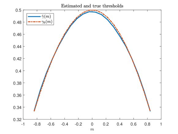
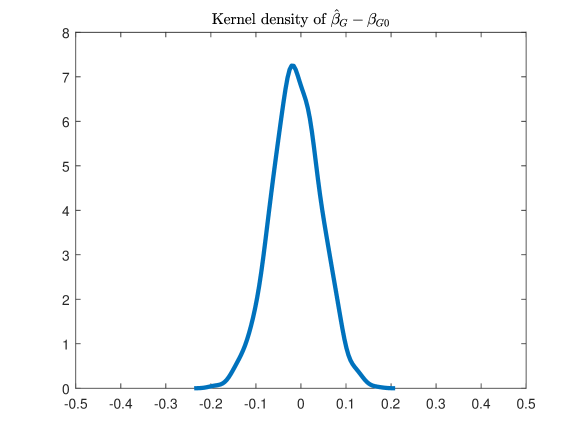
Figure 3 depicts the average of 1,000 estimates against the true function . Figure 4 depicts the kernel density based on the 1,000 estimates , which suggests a good normal approximation. Both figures are based on a sample size of and use the same data-generating process as in the previous tables.
5.2 Endogenous
Our second study examines the estimator when is endogenous. We generate random draws from the following data-generating-process:
where , , and . This model captures the dependence structure that is endogenous and is the valid instrument that is correlated with and uncorrelated with the error term . For this setting, we employ the estimation procedure outlined in Section 4.3. All other parameters are the same as in the simulation setup in the previous subsection.
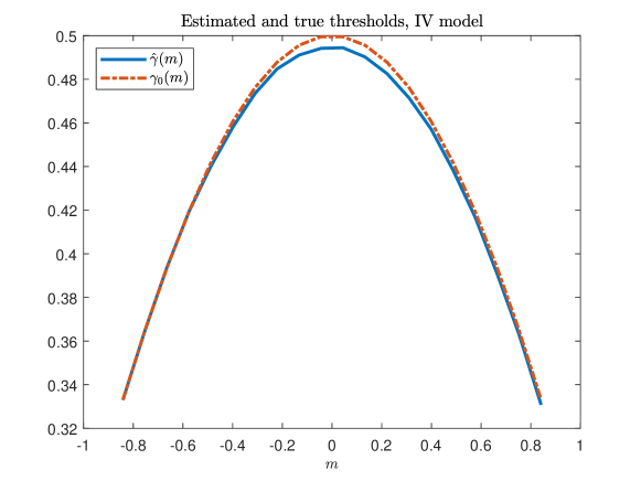
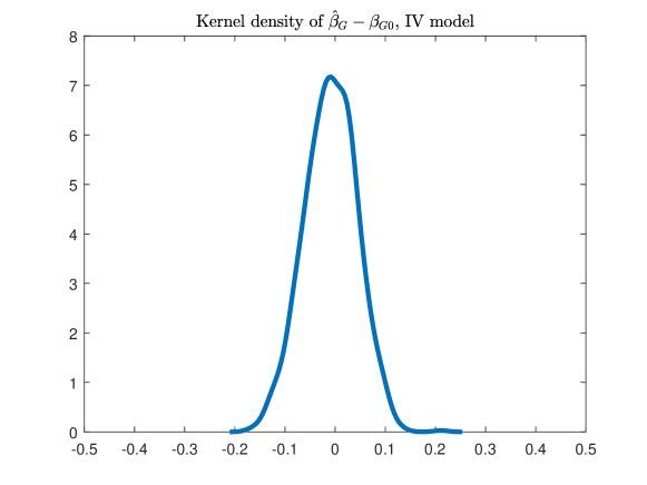
Figures 5 and 6 respectively plot the average estimated threshold function across simulations and the kernel density of the estimated coefficient centered at its true value . Tables 4 and 5 respectively depict the bias and the RMSE of and . The findings are similar to the previous ones without endogeneity. Hence, the proposed estimators permit identification of the threshold (or cutoff) value of the running variable of interest, , as a nonparametric function of , irrespective of whether is exogenous or not. Clearly, the latter requires the availability of relevant and adequate instruments, but this is standard.
| 1 | 2 | 3 | 4 | ||
|---|---|---|---|---|---|
| Bias | 100 | -0.37 | -0.32 | -0.23 | -0.16 |
| 200 | -0.31 | -0.20 | -0.11 | -0.07 | |
| 500 | -0.21 | -0.09 | -0.05 | -0.03 | |
| RMSE | 100 | 0.43 | 0.35 | 0.35 | 0.29 |
| 200 | 0.36 | 0.19 | 0.19 | 0.15 | |
| 500 | 0.24 | 0.09 | 0.09 | 0.08 |
| 1 | 2 | 3 | 4 | 1 | 2 | 3 | 4 | 1 | 2 | 3 | 4 | ||
|---|---|---|---|---|---|---|---|---|---|---|---|---|---|
| Bias | 100 | -0.17 | -0.05 | -0.01 | -0.02 | -0.19 | -0.05 | -0.02 | -0.01 | -0.12 | -0.04 | -0.02 | -0.02 |
| 200 | -0.09 | -0.02 | -0.01 | -0.01 | -0.09 | -0.02 | -0.01 | -0.01 | -0.09 | -0.02 | 0.00 | 0.00 | |
| 500 | -0.01 | 0.01 | 0.00 | 0.00 | -0.03 | -0.01 | 0.00 | -0.01 | -0.04 | 0.01 | 0.00 | 0.00 | |
| RMSE | 100 | 0.72 | 0.39 | 0.23 | 0.16 | 0.81 | 0.40 | 0.24 | 0.17 | 0.76 | 0.48 | 0.32 | 0.25 |
| 200 | 0.62 | 0.27 | 0.14 | 0.11 | 0.63 | 0.29 | 0.16 | 0.12 | 0.68 | 0.36 | 0.21 | 0.16 | |
| 500 | 0.46 | 0.15 | 0.09 | 0.07 | 0.47 | 0.17 | 0.10 | 0.07 | 0.53 | 0.21 | 0.12 | 0.09 | |
6 Empirical Application
6.1 Background
While, along with total and export sales, total profits as well as surrogate variables for fixed costs are readily observable, empirical work on firm selection largely focuses on price data (see Khandelwal,, 2010, Hallak and Sivadasan,, 2013) or sales data and related productivity estimates for identifying threshold effects (see Aw and Hwang,, 1995, Van Biesebroeck,, 2005, Arkolakis,, 2010, Bustos,, 2011, Duan,, 2022, Arkolakis et al.,, 2021). Instead, data on profits are virtually never used in spite of their wide availability from accounting data. We exploit such data for China and describe them in more details in the next subsection.
6.2 Data
We employ data from the Chinese Annual Survey of Industrial Firms (CASIF), which contains accounting data for a large set of companies throughout China. The data are available between 1998 and 2015, but the reporting standards as well as the information provided vary across the years. Because of varying revenue-threshold provisions regarding reporting requirements, the sample sizes of firms differ across the years. As the proposed econometric model involves nonparametric estimation, we prefer data with larger over smaller samples. For that reason, we select data from the year 2008, as the sample size is particularly large in that year.
We apply cleaning steps that are customary prior to using the data (see Upward et al.,, 2013, and Wang and Yu,, 2013, for typical data-cleaning steps with the CASIF data). First, we require total revenues (domestic sales plus exports), export revenues, total profits, financial cost and fixed assets (both alternative measures of total domestic plus exporting fixed costs) to be (i) reported at all and (ii) to be positive for a company.101010We additionally require foreign capital holdings in a firm to take on nonnegative values. Second, there exist some extremely large values for total profits, which compromise the least-squares estimation. Therefore, we trim off the largest 15% of total profits.111111We experimented with alternative trimming thresholds, which led to similar results and findings as reported later. Note that this is not surprising, as one would expect the exporting-threshold productivity or domestic sales not to lie in the right tail of the profit distribution with the data at hand and in general. In any case, such adjustments to avoid the influence of obvious data errors are customary with firm-level data in general. Overall, this leads to a cross-sectional data sample with firms, which we use for estimation.
The dependent variable in our analysis is based on the total profit of firm , . The key threshold- or kink-generating variables are domestic-sales, , and financial-cost measures as surrogate variables for fixed market-access costs, . In this regard, we employ the firm-specific measures Financial costi and Fixed assetsi available in the data. Finally, we consider two variables behind the shifters included in : Rel.for.capitali (relative foreign capital share in total capital of firm ), and Avg.neighb.salesi (the average neighboring firms’ total sales). Rel.for.capitali is included in , because earlier work suggested that foreign-company involvement may affect profits due to profit-shifting, the transfer of technology, etc. Avg.neighb.salesi is included, because close-by firms may induce spillovers. For the latter, we determine a circle with a one-degree diameter around firm and compute the average total sales of other firms therein. It should be noted that those spillovers do not run one-way from other firms to firm but also in the other direction. Therefore, Avg.neighb.salesi should be considered an endogenous regressor and will be in some of the models (see Kelejian and Prucha,, 1998). In any case, we hypothesize that Rel.for.capitali (due to better access to internal finance) and Avg.neighb.salesi (due to knowledge spillovers regarding market access) have the potential of shifting fixed market-access costs.121212Note that one could alternatively consider including such regressors in rather than However, Rel.for.capital is positive for relatively few firms. For that reason, it cannot simply be included as a factor in .
Table 6 presents some summary statistics of the cleaned variables used.131313Beyond what is shown in the table, we could add that 40% of the included companies are exporters and 8% receive foreign capital. With variables in levels as the ones considered here, some regularization is necessary to normalize the large degree of heterogeneity as documented in Table 6.141414The standard deviation is considerably larger than the mean for the continuous variables, and the interquartile range (the distance between the 75th and the 25th quantile, ) attests to large tails in the unnormalized data. This is the case to prevent an excessive degree of heteroskedasticity in estimation and to scale some of the regression parameters. It is customary to log-transform data in international economics – if not the outcome variable, then at least the explanatory ones used in a log-additive index in exponential-family models. However, it should be noted that total profits are (i) additive in levels in a function that is proportional to domestic sales and (ii) governed by a switching function between domestic sellers and exporters. Hence, with this outcome, a log transformation is not useful.
Accordingly, we demean each continuous regressor and normalize the resulting variable by the standard deviation.151515We can normalize the variables in the proposed way without affecting the theoretical relationship for three reasons: (i) the transformations are monotone; (ii) we estimate separate constants to the left and the right of the threshold; and (iii) the threshold set is based on nonparametric estimation which is particularly robust to the transformation of variables. The proposed standardization of variables facilitates the interpretation of the estimated parameters. A one-standard-deviation increase in an included covariate with some parameter then leads to a -fold or change in standardized profits. We refer to the standardized total profits, domestic sales, and financial costs as , , and , respectively. The latter two together generate the set of productivity- or domestic-sales-cutoff parameters for marginal exporters.
Variable Mean Std. Dev. Min Max Variable underlying normalized firm outcome : profits 1,586.29 1,851.77 1.00 253.00 807.00 2254.00 8007.00 Variable underlying normalized firm-level : domestic sales 38,177.35 78,095.16 1.00 9,213.00 19,560.00 43,164.00 7,867,483.00 Variables alternatively underlying normalized firm-level : fixed costs Financial costi 522.73 2,215.06 0.00 15.00 119.00 410.50 254,784.00 Fixed assetsi 11,314.66 54,136.14 1.00 1,539.00 3,882.00 9,595.00 9,207,768.00 Variables underlying as normalized profit shifters in Rel.for.cap.i 0.09 1.53 0.00 0.00 0.00 0.00 349.04 Avg.neighb.salesi 271.25 4,114.29 5.77 14.82 57.46 140.94 822,934.00
-
•
Notes: indexes firms. is total profit (in local currency). Financial cost represents financing costs, and Fixed assets denotes fixed capital assets. Rel.for.cap measures the ratio of foreign asset holdings in total assets of a firm. Avg.neighb.sales is an average of the total sales of other firms in the same circle around firm with one-degree diameter.
6.3 Results
We use the proposed estimator to estimate the set (or contours) of threshold productivities depending on fixed costs with the aforementioned data. For robustness, we consider three different models. Model 1 is the benchmark as in (18),
| (20) |
where are normalized profits, are normalized domestic sales, is one of the two alternative normalized measures of fixed costs (Financial costi or Fixed assetsi) , and includes the foreign capital share relative to total capital (Rel.for.cap.i) and the average of neighboring firms’ total sales (Avg.neighb.salesi). Beyond those variables we include a constant, whose estimate we suppress.
Our second model considers that might be endogenous. After all, the markup charged by companies affects the consumer price and subsequently (domestic as well as foreign) demand. Moreover, local demand shocks will induce simultaneous effects on sales as well as associated profits. How important these sources of endogeneity are for parameter estimation depends on the data and is an empirical question. To address this potential endogeneity, we create two instrumental variables.
The first one we call Demand from firmsi, and it represents an output-share-weighted distance to the potential users of firm ’s output as an input in China’s domestic market. To this end, we use China’s sector-to-sector input-output table for the year 2007 in conjunction with firm-level sales data from CASIF. The latter data contain a sector identifier and permit a mapping of firms to input-output sectors. We assume that a firm in our data is representative of the sector it belongs in. Accordingly, the shares of use sectors of this firm’s output are the same as those of the making sector the firm belongs in. Moreover, we can compute the share each firm other than has in the use sector’s total sales and intermediate purchases. As we have information on each firm’s coordinates based on the spatial information available from CASIF, we can compute firm-to-firm distances. We assume that demand declines with distance in a log-log relationship with a unitary parameter on distance (which is archtypical for gravity relationships). The latter establishes smaller weights in input demand from more distant than from less distant potential input users. Put together, we obtain a weighted input demand from the other firms in CASIF which reflects input-output as well as gravity (distance) aspects in the variable Demand from firmsi. What is key here is that the latter is systematically related to the demand of other companies for firm ’s output without requiring that this prediction is accurate.
Second, we establish a variable called Min.dist.porti, which is the distance of firm to the closest international sea port among the major considered ones.161616The 14 major ports are, in alphabetical order (with rounded latitudes and longitudes in parentheses): Basuo port (lat. 19.0915, lon. 108.6702); Dalian port (lat. 38.9167; lon. 121.6833); Guangzhou port (lat. 23.0939, lon. 113.4378); Haikou port (lat. 20.0526, lon. 20.0526); Nanjing port (lat. 32.2125, lon. 118.8120); Nantong port (lat. 32.0303, lon. 120.8747); Ningbo-Zhoushan port (lat. 29.8667, lon. 121.5500); Qingdao port (lat. 36.0833, lon. 120.3170); Rizhao port (lat. 35.4167, lon. 119.4333); Shanghai port (lat. 31.3664, lon. 121.6147); Shenzhen port (lat. 22.5039, lon. 113.9447); Tianjin port (lat. 38.9727, lon. 117.7845); Xiamen port (lat. 24.5023, lon. 118.0845); and Yingkou port (lat. 40.6936, lon. 122.2662). The latter variable uses two ingredients: (i) the information on the longitude and latitude of firm as already used with the construction of Avg.neighb.salesi as well as Demand from firmsi; and (ii) the information on the longitude and latitude of each one of the Chinese ports mentioned in the previous footnote. We compute the great-circle distance of each firm to each port and pick the shortest one to obtain Min.dist.porti. The latter is a measure of variable export-market-access costs associated with a firm’s location within China. While this variable should directly affect exports, it should matter also for the relative importance of the domestic market for a firm.
We collect these two instrumental variables in the row vector (Demand from firmsi, Min.dist.porti). We use the latter in applying the estimator in Section 4.3 by first regressing on and then adding the residual as an additional regressor in a control-function approach. This leads to our Model 2:
| (21) |
which, except for the control function, is the same as Model 1.
Our third model considers that domestic sales () and the average sales of neighboring firms (Avg.neighb.salesi) are both endogenous. The latter variable’s endogeneity is plausible as neighboring firms’ sales capture peer effects and their relevance indicates the presence of inter-firm (productivity or other) spillovers. Due to circular relationships, weighted other firms’ outcomes will likely induce an estimation bias (see Kelejian and Prucha,, 1998). Accordingly, we regress these two variables on the instruments and obtain the residuals and , respectively, one for each endogenous regressor. Adding both residuals to the kink function, we specify Model 3 as:
| (22) |
which is the same as Model 1, except for the control function. We estimate the threshold first. To this end, we employ the nonparametric regression-kink model (15), using a standard Gaussian kernel with a rule-of-thumb bandwidth in all three models.
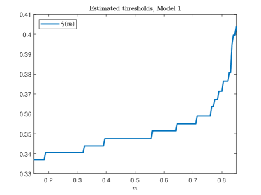
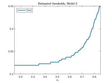
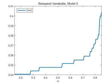
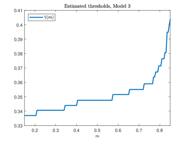
Figure 7 plots the estimated threshold contour based on Model 1 in (20), using Financial costi (left panel) and Fixed assetsi (right panel) as alternative surrogate variables for fixed costs. Both plots exhibit clearly nonlinear and increasing patterns, suggesting that the domestic-sales-threshold increases with higher fixed costs at the firm level, as expected. Figures 8 and 9 display the estimated thresholds based on Models 2 and 3, respectively. All these figures clearly and robustly suggest that the threshold assumes higher domestic-sales values (productivity) for higher fixed costs.171717Let us add that the threshold plots in the figures are not entirely smooth. Such an outcome is typical with nonparametric regression in finite samples since we construct pointwisely. If desired, one could smooth these figures. E.g., it would be desirable to smooth the contours parametrically for use in counterfactual analyses based on quantitative structural models.


Moreover, we report the estimation results for the coefficients for the aforementioned three models, Models 1-3, in Table 7. The interior set in (19) is specified as the interior 98% quantile range of , i.e., . The left panel uses the financial cost as a measure of , and the right panel uses total assets instead.
Let us highlight some interesting findings based on Table 7. First, the coefficient is estimated to be positive and statistically significant, yet smaller than , in Model 1. Hence, the profits of firms to the right of the threshold rise less rather than more with an increase in latent productivity as captured by domestic sales. This evidence contradicts the assumptions and associated results based on customary Melitz-type models. When drawing Figure 1, we assumed that the profits of exporters had a lower intercept (higher total fixed market-access costs) and a steeper slope that non-exporters, aligned with the arguments in Melitz, (2003). The evidence does not support such a mechanism for China, but this is consistent with the aforementioned empirical evidence on the productivity (non-)premium for exporters in China (see Lu et al.,, 2010, 2014; Dai et al.,, 2016). In any case, the results based on Model 1 have to be taken with a grain of salt due to the assumption that domestic sales are deterministic and exogenous. We argued above that this assumption appears strong for plausible reasons.
Second, when relaxing the assumption of exogeneity of and using instrumental-variable estimation through the control-function approach adopted in Models 2 and 3, the evidence of a lack of an exporter productivity or profit premium becomes even stronger. In those models, turns even negative with remaining positive. On the one hand, this aligns with the findings by Lu et al., (2010), Lu et al., (2014), Dai et al., (2016), and Gao and Tvede, (2022) in favor of negative selection. However, it goes beyond those findings in that (allegedly) exporting becomes more likely above if domestic sales and productivity are lower.
Finally, the considered covariates in are positive and statistically different from zero. Hence, the involvement of foreign companies in China tends to boost profits, and there are positive spillovers from neighboring companies’ domestic sales on the average firm . We argued that work in network econometrics suggests that Avg.neighb.salesi acts as a peer-effect term that must be endogenous. The latter is ignored in Models 1 and 2 but not in Model 3. We see that considering the endogeneity of peer effects leads to evidence of considerably larger spillovers than when ignoring it.181818Econometric theory suggests that the peer-effect parameter should be smaller than unity in absolute value, when using weights for other firms that sum up to unity. This is what we find in the two variants of Model 3 as well as in the biased variants of Models 1 and 2. However, the critical threshold for that parameter is not unity here (but lower), due to the normalization of the variables.
All of the mentioned findings are robust to the alternative considered measurements of observable surrogate variables for fixed costs in . The latter can be seen from a comparison of the qualitative findings in the left versus the right block of results in Table 7.
Variable Model 1 Model 2 Model 3 Variable Model 1 Model 2 Model 3 (0.007) (0.007) (0.007) (0.008) (0.033) (0.038) (0.004) (0.008) (0.008) (0.003) (0.031) (0.036) Rel.for.cap.i Rel.for.cap.i (0.002) (0.002) (0.002) (0.003) (0.003) (0.003) Avg.neighb.salesi Avg.neighb.salesi (0.002) (0.002) (0.017) (0.002) (0.002) (0.019) 0.098 0.226 0.232 0.285 0.292 0.300 Observations 187,720 187,720 187,720 Observations 187,720 187,720 187,720
In sum, the results attest to theoretically motivated kinks in the functional relationship between profits and domestic sales, with domestic sales exhibiting a monotone, positive mapping with latent firm productivity. Moreover, the kink is not a point but a contour. This will generally be the case whenever not only one running variable (productivity or any monotone reflection of it) but also another variable such as fixed market-access costs is firm-specific and sufficiently independent of the first running variable.
6.4 Discussion
The estimation approach and empirical analysis in this paper were inspired by and targeting exporter productivity cutoffs. It is useful to draw the reader’s attention to the fact that the only instance where export data had been used up until now was to construct the domestic-sales variable and its normalized counterpart . But export data (neither in binary nor continuous form) had not been used in the estimation. However, ex post it is useful to bring exports to the fore in the interest of providing background for differences in the firms’ propensity to export on the two sides of the threshold.
Recall the discussion in Melitz, (2003) as well as the illustration in Figure 1. With positive firm selection (i.e., with more productive and larger domestic sellers selecting into exporting), all or most firms to the right of the threshold (above-cutoff productivity and domestic sales) would be exporters and all or most to the left would be non-exporters. Stochastic profit shocks as well as heterogeneous fixed costs (or other fundamentals) generate some fuzziness about this pattern but the qualitative result would persist. If the profit function of domestic sellers would be steeper than the one of exporters and exporting fixed costs would be stochastically dominated by domestic market-access costs, we could have negative selection. Then, exporters would be found more likely below the cutoff productivity and domestic sales than above.
We commented earlier that the finding of a slope parameter on normalized domestic sales above the threshold of with a positive parameter on normalized domestic sales below the threshold, , is consistent with a negative selection of firms into exporting in China. We also said that a negative parameter is in stark contrast with the expectations formed against the backdrop of the customary assumptions adopted by Melitz, (2003) regarding firm selection.
Let us now benchmark the latter finding and conclusion with the probability of exporting above and below the estimated threshold. We do so by generating a -percentile grid on both sides of the threshold contour in - space. Then we determine the fraction of exporters in the ppt. cells. We illustrate the findings in Figure 10.
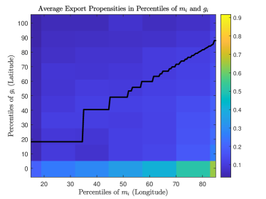
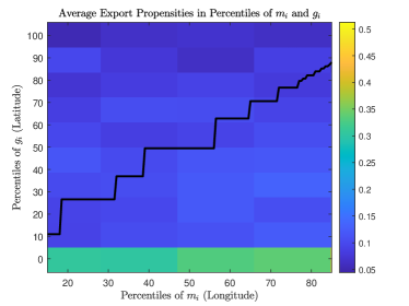
Figure 10 contains two panels, depending on the use of surrogate variables for fixed costs in . The one on the left employs quantiles of Financial costi, and the on on the right employs Fixed assetsi. We use lighter colors for higher exporter fractions (propensities) and darker ones for lower ones.
In line with data, essentially for all countries we know of, exporters occur in a wide domain of domestic sales and surrogate variables for fixed costs. Hence, selection is fuzzy rather than sharp. Moreover, we see that exporters are particularly prevalent in the lowest decile of domestic sales, . This observation is consistent with earlier-cited work on China (see Lu,, 2010, Lu et al.,, 2010, Lu et al.,, 2014, and Gao and Tvede,, 2022). On average, exporters are least prevalent in the lowest- decile and the higher deciles in the left panel and and in the lower- and higher- deciles in the right panel. The main take-away message is that exporters are less frequent below (to the left of) the cutoff than above (to the right of) the estimated threshold. Hence, exporters emerge less likely in a higher-domestic-sales and lower-fixed-cost environment than in a lower-domestic-sales and higher-fixed-cost environment. This suggests that the assumptions generating positive selection are violated in China. And government or foreign-firm interference may be at the roots of this pattern.
7 Conclusions
This paper introduces a novel framework to estimate productivity thresholds in firm models of international trade. Specifically, the estimation framework allows for more than one dimension of firm heterogeneity as it is commonly encountered in data but rarely addressed in economic theory (see Arkolakis,, 2010, Helpman et al.,, 2016, or Adão et al.,, 2020, for exceptions): productivity and fixed costs. In principal, the framework would be capable of considering even more than two such dimensions. In any setting, where productivity (or another heterogeneous variable) is not the single firm-indexed parameter, and firms make choices about discrete alternatives such as exporting or not, the critical value of the firm parameter (e.g., the exporter cutoff productivity) is not scalar- but set-valued.
Moreover, the (scaled) firm productivity is proportional to several observable outcomes such as prices or domestic sales. But fixed costs or other firm-specific attributes are not clearly parametrically related to observable surrogate variables thereof. For that reason, we develop the estimator as to combine parametric and non-parametric forms in the threshold-generation function. We prove the large-sample properties of the estimator and document its suitability in finite samples by simulation.
Using a large cross section of non-exporting and exporting firms in China, we document that productivity-threshold estimates are indeed not constant but vary systematically with fixed costs. As theory predicts, firms which have higher fixed market-entry costs require a higher productivity to survive and make profits. The variation of fixed costs across firms is large and this translates into a large variation of the set of productivity thresholds. This translation is not mechanical, as we permit the relationship to be nonparametric. We consider this evidence as particularly strong and more powerful than what one could obtain from parametric estimates (e.g., ones based on interaction effects).
Our results have broader implications for international trade theory and policy. E.g., trade-cost or market-size shocks do not trigger effects and responses primarily and only in the left tail of the firm-size distribution. Depending on the covariance structure between productivity and fixed costs among firms, trade-cost shocks will affect firms in a large support area of their size distribution. E.g., tariff increases as envisaged by the Trump II administration have the potential of triggering significant exit of medium-sized and even large firms from exporting, if productivity and fixed costs are positively correlated. We find the latter to be the case with the data at hand. On the contrary, trade-liberalization events might lead to an entry of large enterprises in a market which they did not find attractive before, because of high firm-specific fixed entry costs.
We used the consideration of the choice between exporting and non-exporting in a context of firm-specific productivity and fixed costs as a guiding example. As argued in the paper, the benchmarking of some operating profits or other variable gains against some fixed costs is a fairly generic problem in international economics and industrial organization alike. Many contexts there involve discrete choices of companies and lead to subsets of companies choosing one alternative over another. Apart from export-market entry closely-related problems include the adoption of new (single or multiple) products, the set up of (domestic or foreign) affiliates, the integration of suppliers or buyers, etc. The search for kinks or breaks or cutoff values of fundamental running variables in the functional relationships with such problems is of a generic importance in those contexts. A natural stochastic approach to identify these cutoff or breakpoints in running variables is the kink-regression framework. If more than a single variable (such as productivity) has threshold-generating power but there is at least one more determinant, the threshold does not degenerate to a point but is an at least two-dimensional contour. Whenever the surrogate variables of fixed costs of adopting an alternative strategy (exporting, multi-plant production, multinational production, outsourcing or offshoring, integration of suppliers or buyers, etc.) are measured with some variation across firms, one is faced with exactly this problem. And in absence of a tight theoretical guidance on the mapping of surrogate variables to fixed costs or other firm-specific parameters, one would then wish to permit a nonparametric relationship between observables and theoretical fixed costs underlying firms’ choices. The present paper provides an estimation framework for exactly such problems.
Future research could extend the proposed methodology to dynamic settings or investigate its applicability to other economic contexts, where firm heterogeneity plays a critical role. Examples are settings where firms choose multinomially to produce a set of products (multi-product firms) or firms choose multinomially to set up plants (multi-plant or multinational firms).
Appendix A Proof
Proof of Theorem 1.
Since the proof is pointwise in , we use the short-handed notation for simplicity. For any constant with given , we define a conditional -loss as
which is continuous in . By construction, for any and . Hence, it suffices to show that for any vector given . To this end, we split the event into two disjoint cases: (i) regardless of ; or (ii) but . These two cases are comprehensive.
For case (ii), we consider without loss of generality. Note that
where the last probability is strictly positive because and from Assumption 1.3. ∎
Proof of Theorem 2.
Recall that
where
and
Define
which is a row-wise i.i.d. triangular array. We aim to show that
| (28) |
Then, the consistency follows from Theorem 1, Lemma 1, and the standard argument (e.g., Amemiya Theorem 4.1.1). Since is a quadratic function of , the only issue is establishing the stochastic equicontinuity with respect to . We thus simplify the notation by writing and illustrate with . Moreover, since we focus on a fixed , we write for simplicity. It suffices to check the following three steps. Then (28) follows by checking the conditions of Theorem 2.8.1 of Van der Vaart and Wellner (1996).
1. is Lipschtiz continuous with constant .
2. and are dominated by a function
3. .
For 1, without loss of generality, Then
For 2, set
Then
For 3, since is continuous. Then
which holds uniformly over .
∎
Proof of Theorem 3.
Recall that approximately solves the first-order condition
| (30) | |||||
for some intermediate value , where we denote and
It remains to show that (i).; (ii). ; and (iii) .
For (i), note that is a row-wise i.i.d. triangular array with zero mean. Its variance satisfies that
Then (i) follows from the triangular array central limit theorem.
For (ii), the same argument as in Lemma 1 yields that
which is now differentiable w.r.t. . Then (ii) follows from the consistency, i.e., Theorem 2.
For (iii), denoting
it suffices to show the stochastic equicontinuity of , i.e., for any , there exists such that
| (31) |
By Cauchy-Schwartz inequality and Assumption 1.2,
The above bound is uniform over and hence (31) follows from Chebyshev’s inequality. The proof is complete by combining (i)-(iii).
∎
Proof of Theorem 4.
The proof consists of three steps.
Step 1: Establish the uniform convergence
| (33) |
To this end, recall the notation . With slightly abused notation, we denote and . The proof of Theorem 3 yields that
where are as in (30). For , standard argument (e.g., Li and Racine, 2006, Chapter 1) implies that , which is provided that for (Assumption 2.3). For , a similar argument for establishing (28) yields that uniformly over . For , the argument in the proof of Theorem 3 yields that , which is again . Then (33) follows from combining .
Step 2: By the continuous mapping theorem and the law of large numbers, we have
Also, by the standard central limit theorem,
Step 3: Establish that
which is implied by is continuous in and Step 1. The proof is complete by combining steps 1-3.
∎
References
- Adão et al., (2020) Adão, R., Arkolakis, C., and Ganapati, S. (2020). Aggregate implications of firm heterogeneity: A nonparametric analysis of monopolistic competition trade models. Technical report, National Bureau of Economic Research.
- Alfaro et al., (2019) Alfaro, L., Chor, D., Antràs, P., and Conconi, P. (2019). Internalizing global value chains: A firm-level analysis. Journal of Political Economy, 127(2):508–559.
- Alfaro-Urena et al., (2022) Alfaro-Urena, A., Manelici, I., and Vasquez, J. P. (2022). The effects of joining multinational supply chains: New evidence from firm-to-firm linkages. Quarterly Journal of Economics, 137(3):1495–1552.
- Antràs, (2005) Antràs, P. (2005). Property rights and the international organization of production. American Economic Review, 95(2):25–32.
- Antràs and Helpman, (2004) Antràs, P. and Helpman, E. (2004). Global sourcing. Journal of Political Economy, 112(3):552–580.
- Arkolakis, (2010) Arkolakis, C. (2010). Market penetration costs and the new consumers margin in international trade. Journal of political economy, 118(6):1151–1199.
- Arkolakis et al., (2021) Arkolakis, C., Ganapati, S., and Muendler, M.-A. (2021). The extensive margin of exporting products: A firm-level analysis. American Economic Journal: Macroeconomics, 13(4):182–245.
- Aw and Hwang, (1995) Aw, B. Y. and Hwang, A. R. (1995). Productivity and the export market: A firm-level analysis. Journal of Development Economics, 47(2):313–332.
- Baltagi et al., (2016) Baltagi, B. H., Egger, P. H., and Kesina, M. (2016). Firm-level productivity spillovers in china’s chemical industry: A spatial hausman-taylor approach. Journal of Applied Econometrics, 31(1):214–248.
- Becker et al., (2013) Becker, S. O., Egger, P. H., and Von Ehrlich, M. (2013). Absorptive capacity and the growth and investment effects of regional transfers: A regression discontinuity design with heterogeneous treatment effects. American Economic Journal: Economic Policy, 5(4):29–77.
- Bernard et al., (2003) Bernard, A. B., Eaton, J., Jensen, J. B., and Kortum, S. (2003). Plants and productivity in international trade. American Economic Review, 93(4):1268–1290.
- Bernard and Jensen, (1999) Bernard, A. B. and Jensen, J. B. (1999). Exceptional exporter performance: cause, effect, or both? Journal of International Economics, 47(1):1–25.
- Bernard and Jensen, (2004) Bernard, A. B. and Jensen, J. B. (2004). Why some firms export. Review of Economics and Statistics, 86(2):561–569.
- Bernard et al., (2007) Bernard, A. B., Jensen, J. B., Redding, S. J., and Schott, P. K. (2007). Firms in international trade. Journal of Economic Perspectives, 21(3):105–130.
- Bernard et al., (2012) Bernard, A. B., Jensen, J. B., Redding, S. J., and Schott, P. K. (2012). The empirics of firm heterogeneity and international trade. Annual Review of Economics, 4:283–313.
- Bernard et al., (2010) Bernard, A. B., Van Beveren, I., and Vandenbussche, H. (2010). Multi-product exporters, carry-along trade and the margins of trade. Tuck School of Business Working Paper, (2011-91).
- Bustos, (2011) Bustos, P. (2011). Trade liberalization, exports, and technology upgrading: Evidence on the impact of mercosur on argentinian firms. American Economic Review, 101(1):304–340.
- (18) Card, D., Johnston, A., Leung, P., Mas, A., and Pei, Z. (2015a). The effect of unemployment benefits on the duration of unemployment insurance receipt: New evidence from a regression kink design in missouri, 2003–2013. American Economic Review, 105(5):126–130.
- (19) Card, D., Lee, D. S., Pei, Z., and Weber, A. (2015b). Inference on causal effects in a generalized regression kink design. Econometrica, 83(6):2453–2483.
- Chaney, (2008) Chaney, T. (2008). Distorted gravity: the intensive and extensive margins of international trade. American Economic Review, 98(4):1707–1721.
- Dai et al., (2016) Dai, M., Maitra, M., and Yu, M. (2016). Unexceptional exporter performance in china? the role of processing trade. Journal of Development Economics, 121:177–189.
- Duan, (2022) Duan, L. (2022). Estimation of export cutoff productivity of chinese industrial enterprises. PLOS ONE, 17(11):1–16.
- Eaton and Kortum, (2002) Eaton, J. and Kortum, S. (2002). Technology, geography, and trade. Econometrica, 70(5):1741–1779.
- Egger and Erhardt, (2024) Egger, P. H. and Erhardt, K. (2024). Heterogeneous effects of tariff and nontariff trade-policy barriers in quantitative general equilibrium. Quantitative Economics, 15(2):453–487.
- Egger and Koethenbuerger, (2010) Egger, P. H. and Koethenbuerger, M. (2010). Government spending and legislative organization: Quasi-experimental evidence from germany. American Economic Journal: Applied Economics, 2(4):200–212.
- Egger and Lassmann, (2015) Egger, P. H. and Lassmann, A. (2015). The causal impact of common native language on international trade: Evidence from a spatial regression discontinuity design. Economic Journal, 125(584):699–745.
- Gao and Tvede, (2022) Gao, B. and Tvede, M. (2022). The impact of trade with pure exporters. Review of International Economics, 30(1):83–112.
- Gonzalez, (2021) Gonzalez, R. M. (2021). Cell phone access and election fraud: evidence from a spatial regression discontinuity design in afghanistan. American Economic Journal: Applied Economics, 13(2):1–51.
- Hahn et al., (2001) Hahn, J., Todd, P., and Van der Klaauw, W. (2001). Identification and estimation of treatment effects with a regression-discontinuity design. Econometrica, 69(1):201–209.
- Hallak and Sivadasan, (2013) Hallak, J. C. and Sivadasan, J. (2013). Product and process productivity: Implications for quality choice and conditional exporter premia. Journal of International Economics, 91(1):53–67.
- Hansen, (2000) Hansen, B. E. (2000). Sample splitting and threshold estimation. Econometrica, 68(3):575–603.
- Hansen, (2017) Hansen, B. E. (2017). Regression kink with an unknown threshold. Journal of Business & Economic Statistics, 35(2):228–240.
- Head et al., (2014) Head, K., Mayer, T., and Thoenig, M. (2014). Welfare and trade without pareto. American Economic Review, 104(5):310–316.
- Helpman et al., (2016) Helpman, E., Itskhoki, O., Muendler, M.-A., and Redding, S. J. (2016). Trade and inequality: From theory to estimation. Review of Economic Studies, 84(1):357–405.
- Helpman et al., (2004) Helpman, E., Melitz, M. J., and Yeaple, S. R. (2004). Export versus fdi with heterogeneous firms. American Economic Review, 94(1):300–316.
- Hess et al., (2010) Hess, K., Gunasekarage, A., and Hovey, M. (2010). State-dominant and non-state-dominant ownership concentration and firm performance: Evidence from china. International Journal of Managerial Finance, 6(4):264–289.
- Hillberry and Hummels, (2008) Hillberry, R. and Hummels, D. (2008). Trade responses to geographic frictions: A decomposition using micro-data. European Economic Review, 52(3):527–550.
- Hopenhayn, (1992) Hopenhayn, H. A. (1992). Entry, exit, and firm dynamics in long run equilibrium. Econometrica, pages 1127–1150.
- Jørgensen and Schröder, (2008) Jørgensen, J. G. and Schröder, P. J. (2008). Fixed export cost heterogeneity, trade and welfare. European Economic Review, 52(7):1256–1274.
- Kelejian and Prucha, (1998) Kelejian, H. H. and Prucha, I. R. (1998). A generalized spatial two-stage least squares procedure for estimating a spatial autoregressive model with autoregressive disturbances. Journal of Real Estate Finance and Economics, 17:99–121.
- Khandelwal, (2010) Khandelwal, A. (2010). The long and short (of) quality ladders. Review of Economic Studies, 77(4):1450–1476.
- Landais, (2015) Landais, C. (2015). Assessing the welfare effects of unemployment benefits using the regression kink design. American Economic Journal: Economic Policy, 7(4):243–278.
- Lazzarini and Musacchio, (2018) Lazzarini, S. G. and Musacchio, A. (2018). State ownership reinvented? explaining performance differences between state-owned and private firms. Corporate Governance: An International Review, 26(4):255–272.
- Lu, (2010) Lu, D. (2010). Exceptional exporter performance? evidence from chinese manufacturing firms. manuscript, University of Chicago.
- Lu et al., (2010) Lu, J., Lu, Y., and Tao, Z. (2010). Exporting behavior of foreign affiliates: Theory and evidence. Journal of International Economics, 81(2):197–205.
- Lu et al., (2014) Lu, J., Lu, Y., and Tao, Z. (2014). Pure exporter: Theory and evidence from china. World Economy, 37(9):1219–1236.
- Manova, (2008) Manova, K. (2008). Credit constraints, equity market liberalizations and international trade. Journal of International Economics, 76(1):33–47.
- Manova, (2013) Manova, K. (2013). Credit constraints, heterogeneous firms, and international trade. Review of Economic Studies, 80(2):711–744.
- Melitz, (2003) Melitz, M. J. (2003). The impact of trade on intra-industry reallocations and aggregate industry productivity. Econometrica, 71(6):1695–1725.
- Nocke and Yeaple, (2014) Nocke, V. and Yeaple, S. (2014). Globalization and multiproduct firms. International Economic Review, 55(4):993–1018.
- Ouyang et al., (2015) Ouyang, P., Zhang, T., and Dong, Y. (2015). Market potential, firm exports and profit: Which market do the chinese firms profit from? China Economic Review, 34:94–108.
- Seo and Linton, (2007) Seo, M. H. and Linton, O. (2007). A smoothed least squares estimator for threshold regression models. Journal of Econometrics, 141(2):704–735.
- Upward et al., (2013) Upward, R., Wang, Z., and Zheng, J. (2013). Weighing china’s export basket: The domestic content and technology intensity of chinese exports. Journal of Comparative Economics, 41(2):527–543.
- Van Biesebroeck, (2005) Van Biesebroeck, J. (2005). Exporting raises productivity in sub-saharan african manufacturing firms. Journal of International Economics, 67(2):373–391.
- Wang and Yu, (2013) Wang, Z. and Yu, Z. (2013). Trading partners, traded products and firm performances of china’s exporterimporters: Does processing trade make a difference? World Economy, pages 165–193.
- Zhang et al., (2024) Zhang, J., Chen, C., Sun, Y., and Stengos, T. (2024). Endogenous kink threshold regression. Journal of Business & Economic Statistics, pages 1–12.