Revisiting Stochastic Proximal Point Methods:
Generalized Smoothness and Similarity

Abstract

The growing prevalence of nonsmooth optimization problems in machine learning has spurred significant interest in generalized smoothness assumptions. Among these, the $(L_{0},L_{1})$-smoothness assumption has emerged as one of the most prominent. While proximal methods are well-suited and effective for nonsmooth problems in deterministic settings, their stochastic counterparts remain underexplored. This work focuses on the stochastic proximal point method (SPPM), valued for its stability and minimal hyperparameter tuning—advantages often missing in stochastic gradient descent (SGD). We propose a novel $\phi$-smoothness framework and provide a comprehensive analysis of SPPM without relying on traditional smoothness assumptions. Our results are highly general, encompassing existing findings as special cases. Furthermore, we examine SPPM under the widely adopted expected similarity assumption, thereby extending its applicability to a broader range of scenarios. Our theoretical contributions are illustrated and validated by practical experiments.

1 Introduction

In this paper, we address the stochastic optimization problem of minimizing the expected function

$$\min_{x\in\mathbb{R}^{d}}\big{\{}f(x):=\mathbb{E}_{\xi\sim\mathcal{D}}\left[f_{\xi}(x)\right]\big{\}},$$ (1)

where $\xi\sim\mathcal{D}$ is a random variable drawn from the distribution $\mathcal{D}$, and $\mathbb{E}[\cdot]$ represents the mathematical expectation. Here, $x$ represents a machine learning (ML) model with $d$ parameters, $\mathcal{D}$ denotes the distribution of labeled examples, $\xi\sim\mathcal{D}$ are the samples, $f_{\xi}$ represents the loss associated with a single sample $\xi$, and $f$ corresponds to the generalization error. In this setting, while an unbiased estimator of the gradient $\nabla f_{\xi}(x)$ can be computed, the gradient $\nabla f(x)$ itself is not directly accessible. Such problems form the backbone of supervised learning theory (Bottou et al., 2018; Sun et al., 2019; Sun, 2020).

A particular case of interest is the finite-sum optimization problem, where $f$ is the average of a large number of functions (Agarwal & Bottou, 2015; Schmidt et al., 2017):

$$\min_{x\in\mathbb{R}^{d}}\left\{f(x):=\frac{1}{n}\sum_{i=1}^{n}f_{i}(x)\right\}.$$ (2)

This problem frequently arises when training supervised ML models using empirical risk minimization (Feldman, 2016; Gambella et al., 2021). It is an instance of (1) with $\mathcal{D}$ the uniform distribution over the finite set $\{1,\ldots,n\}$.

Optimization problems in ML and Deep Learning (DL) are frequently nonsmooth, meaning that the gradient of the objective function does not necessarily satisfy the Lipschitz continuity condition, or is even not well defined (Iutzeler & Malick, 2020; Gorbunov et al., 2024). For instance, even in relatively simple neural networks, the gradient of the standard $\ell_{2}$-regression loss fails to satisfy Lipschitz continuity (Zhang et al., 2019). Moreover, the convex but nonsmooth setting often provides an effective framework for capturing the complexities of DL problems (Khaled et al., 2023). Many widely used and empirically successful adaptive optimization algorithms, such as AdaGrad (Duchi et al., 2011), Adam (Kingma, 2014), and Prodigy (Mishchenko & Defazio, 2023) have been specifically designed for this setting, demonstrating their practical effectiveness across various DL applications.

In contrast, optimization methods that rely on smoothness assumptions and offer strong theoretical guarantees frequently fall short in practical DL tasks (Crawshaw et al., 2022). For example, while variance-reduced methods (Reddi et al., 2016; Gower et al., 2020) achieve superior convergence rates in theory, they are often outperformed by simpler methods in practice due to the challenges posed by the complex and highly nonconvex landscapes of DL (Defazio & Bottou, 2019). These challenges have motivated researchers to introduce more realistic smoothness assumptions and develop corresponding theoretical guarantees within these refined frameworks (Vankov et al., 2024; Gorbunov et al., 2024).

One of the earliest extensions beyond the standard Lipschitz smoothness assumption is the $\boldsymbol{(L_{0},L_{1})}$-smoothness condition, which was initially proposed for twice-differentiable functions (Zhang et al., 2019). This assumption posits that the norm of the Hessian can be bounded linearly by the norm of the gradient. Later, this assumption was generalized to encompass a broader class of differentiable functions (Zhang et al., 2020; Chen et al., 2023).

Stochastic Gradient Descent (SGD) methods have been extensively analyzed in both convex and nonconvex settings, with significant attention also given to adaptive variants and other modifications (Zhao et al., 2021; Faw et al., 2023; Wang et al., 2023; Hübler et al., 2024b). A natural extension of the $(L_{0},L_{1})$-smoothness assumption involves bounding the Hessian norm with a polynomial dependence on the gradient norm, offering a more flexible and generalized formulation. A further and even more general approach to smoothness involves the use of an arbitrary nondecreasing continuous function to bound the Hessian norm (Li et al., 2024b). This generalized setting not only encompasses the previously discussed assumptions but also provides a broader and more adaptable framework applicable to a wide range of functions (Tyurin, 2024).

While SGD methods have been extensively studied in the context of generalized smoothness, stochastic proximal point methods (SPPM) remain relatively underexplored. SPPM can serve as an effective alternative when stochastic proximity operators are computationally feasible (Asi & Duchi, 2019; Asi et al., 2020; Khaled & Jin, 2022). We recall that the proximity operator (prox) of a function $f:\mathbb{R}^{d}\rightarrow\mathbb{R}\cup\{+\infty\}$ is

$$\mathrm{prox}_{f}(x)\stackrel{{\scriptstyle\text{def}}}{{=}}\underset{z\in\mathbb{R}^{d}}{\mathrm{argmin}}\left\{f(z)+\frac{1}{2}\|z-x\|^{2}\right\}$$ (3)

(Bauschke et al., 2017). Proximal methods, which leverage proxs of functions (Parikh & Boyd, 2014; Condat et al., 2023b), are known for their robustness and resilience to the choice of stepsize, often allowing for the use of larger stepsizes compared to standard gradient-based methods. Ryu & Boyd (2014) provide convergence rate guarantees for SPPM and emphasize its stability with respect to inaccuracies in learning rate selection; a property not typically observed in SGD. Asi & Duchi (2019) investigate a more general framework, AProx, which encompasses SPPM as a special case. They establish both stability and convergence rate results for AProx under convexity assumptions. Moreover, SPPM has been shown to achieve convergence rates comparable to those of SGD across a variety of algorithmic settings (Richtárik et al., 2024).

Alternatively, instead of relying on the smoothness assumption and its generalizations, we can consider the similarity assumption (Shamir et al., 2014). It reflects the idea that there is a certain level of similarity or homogeneity among the gradients, which is particularly relevant in ML, where these gradients capture the characteristics of the underlying data (Goodfellow, 2016; Sun et al., 2022). Recognizing this natural property, several recent works have explored various formulations and generalizations of the similarity assumption (Hendrikx et al., 2020; Szlendak et al., 2021; Sadiev et al., 2024). In particular, multiple studies have analyzed stochastic proximal methods under different similarity conditions, demonstrating their practical relevance and theoretical significance (Gasanov & Richtarik, 2024; Sadiev et al., 2024). Moreover, the concept of similarity offers a more refined perspective on the behavior of optimization algorithms in distributed and federated learning settings (Karimireddy et al., 2020; Kovalev et al., 2022; Jiang et al., 2024b).

To make the considered methods practical, the computation of a prox often involves an inexact approach, where it is approximated by several iterations of a subroutine designed to solve the corresponding auxiliary problem. This technique has been extensively studied in the literature, with various criteria established to ensure the effectiveness of the approximation (Kovalev et al., 2022; Grudzień et al., 2023a; Borodich et al., 2023). These criteria typically include conditions such as relative and absolute error thresholds (Khaled & Jin, 2022; Li & Richtárik, 2024), as well as guarantees on the reduction of the gradient norm (Sadiev et al., 2022). Meeting these criteria is crucial to maintaining the overall convergence properties and efficiency of the optimization algorithm while balancing computational cost and accuracy.

Our contributions are the following.

• New generalized smoothness assumption, called $\boldsymbol{\phi}$-smoothness. We investigate the most general conditions required for the convergence of SPPM and introduce the novel notion of $\phi$-smoothness (Section 4). Under this assumption, we establish rigorous convergence guarantees and explore various special cases, highlighting the specific effects and implications of the proposed framework.

• Convergence under $\phi$-smoothness. We conduct a comprehensive analysis of SPPM when the prox is computed inexactly under the newly introduced $\phi$-smoothness assumption (Section 5). Specifically, we derive conditions on the number of subroutine steps required to solve the auxiliary problem, ensuring that the overall iteration complexity remains the same as in the case of exact proximal evaluations. Our results provide practical guidelines for balancing computational efficiency and theoretical guarantees. Our convergence analysis covers both strongly convex and general convex settings, and we precisely characterize the convergence rates, offering insights into the tradeoffs between problem complexity and algorithmic performance.

• Convergence under expected similarity. We further extend our theoretical contributions to settings with the expected similarity assumption (Section 6), which captures practical scenarios where the different functions share a certain degree of similarity in expectation. Under this assumption, we derive specific convergence results, offering valuable theoretical insights.

• Experiments. To support our theoretical findings, we conduct a series of carefully designed experiments that empirically validate our predictions and provide deeper insights into the practical performance of the proposed methods (Section 7).

2 Preliminaries

Before presenting our convergence results, we define the key concepts and outline the assumptions used throughout the work. We start with the standard assumptions that apply to all our results, primarily that each stochastic function $f_{\xi}$ is convex and differentiable (for simplicity, to avoid complicated notations associated to set-valued subdifferentials, see their use in Sadiev et al. (2024))

Assumption 2.1 (Differentiability).

The function $f_{\xi}:\mathbb{R}^{d}\to\mathbb{R}$ is differentiable for $\mathcal{D}$-almost every sample $\xi$.

We implicitly assume that differentiation and expectation can be interchanged, which leads to $\nabla f(x)=\nabla\mathbb{E}_{\xi\sim\mathcal{D}}\left[f_{\xi}(x)\right]=\mathbb{E}_{\xi\sim\mathcal{D}}\left[\nabla f_{\xi}(x)\right]$. Consequently, $f$ is differentiable.

Assumption 2.2 (Convexity).

The function $f_{\xi}:\mathbb{R}^{d}\to\mathbb{R}$ is convex for $\mathcal{D}$-almost every sample $\xi$; that is,

$$f_{\xi}(x)\geq f_{\xi}(y)+\langle\nabla f_{\xi}(y),x-y\rangle\quad\forall x,y\in\mathbb{R}^{d}.$$

Next, we formulate the strong convexity assumption, which is applied to the expected function $f$ in several settings:

Assumption 2.3 (Strong convexity of $f$).

The function $f:\mathbb{R}^{d}\to\mathbb{R}$ is $\mu$-strongly convex for some $\mu>0$; that is,

$$f(x)\geq f(y)+\langle\nabla f(y),x-y\rangle+\frac{\mu}{2}\|x-y\|^{2}\quad\forall x,y\in\mathbb{R}^{d}.$$

A strongly convex function is better behaved and easier to minimize than a merely convex one.

Next, we consider the interpolation condition, where all stochastic functions share a common minimizer. This regime is commonly observed in overparameterized models, particularly large-scale ML models, where the number of parameters exceeds the number of training examples, enabling perfect fit to the data (Ma et al., 2018; Varre et al., 2021).

Assumption 2.4 (Interpolation regime).

There exists $x_{\star}\in\mathbb{R}^{d}$ such that $\nabla f_{\xi}(x_{\star})=0$ for $\mathcal{D}$-almost every sample $\xi$.

Now we need to formulate several smoothness assumptions which are used in the analysis. We start with the well-known standard assumption of $L$-smoothness:

Assumption 2.5 ($L$-smoothness).

The function $f_{\xi}\colon\mathbb{R}^{d}\to\mathbb{R}$ is $L$-smooth for $\mathcal{D}$-almost every sample $\xi$; that is, it is differentiable and its gradient is $L$-Lipschitz continuous:

$$\|\nabla f_{\xi}(x)-\nabla f_{\xi}(y)\|\leq L\|x-y\|\quad\forall x,y\in\mathbb{R}^{d}.$$

Next, we introduce the $(L_{0},L_{1})$-smoothness assumption, initially formulated by Zhang et al. (2020).

Assumption 2.6 (Symmetric $(L_{0},L_{1})$-smoothness ).

The function $f_{\xi}\colon\mathbb{R}^{d}\to\mathbb{R}$ is symmetrically $(L_{0},L_{1})$-smooth for $\mathcal{D}$-almost every sample $\xi$; that is,

$$\|\nabla f_{\xi}(x)-\nabla f_{\xi}(y)\|\leq\left(L_{0}+L_{1}\sup_{u\in[x,y]}\|\nabla f_{\xi}(u)\|\right)\|x-y\|\quad\forall x,y\in\mathbb{R}^{d},$$

where $[x,y]$ is the interval connecting the points $x$ and $y$.

A more generalized form of symmetric $(L_{0},L_{1})$-smoothness is the so-called $\alpha$-symmetric generalized smoothness, introduced by Chen et al. (2023). This extension provides a more flexible framework for analyzing smoothness properties by incorporating an additional parameter $\alpha$, which allows for a broader class of functions to be captured within the smoothness definition.

Assumption 2.7 ($\alpha$-symmetric generalized smoothness).

The function $f_{\xi}\colon\mathbb{R}^{d}\to\mathbb{R}$ is $\alpha$-symmetrically generalized-smooth for $\mathcal{D}$-almost every sample $\xi$; that is,

$$\|\nabla f_{\xi}(x)-\nabla f_{\xi}(y)\|\leq\left(L_{0}+L_{1}\sup_{u\in[x,y]}\|\nabla f_{\xi}(u)\|^{\alpha}\right)\|x-y\|\quad\forall x,y\in\mathbb{R}^{d},$$

where $\alpha\in[0,1]$ and $[x,y]$ is the interval connecting the points $x$ and $y$.

It is important to note that when $\alpha=0$, the definition reduces to the standard $L$-smoothness, and when $\alpha=1$, it corresponds to the symmetric $(L_{0},L_{1})$-smoothness.

Then we consider the expected similarity assumption. Initially, the concept of similarity was introduced for twice-differentiable functions and is commonly referred to as Hessian similarity (Tian et al., 2022). For functions that are only once differentiable, analogous assumptions have been employed in the literature. In this work, we propose an even more general assumption introduced by Sadiev et al. (2024). We call it Star Similarity since it only has to hold with respect to a solution $x_{\star}$.

Assumption 2.8 (Star Similarity).

The function $f_{\xi}\colon\mathbb{R}^{d}\to\mathbb{R}$ has Star Similarity; that is, there exist a solution $x_{\star}$ of (1) and a constant $\delta_{\star}>0$ such that

$$\mathbb{E}_{\xi\sim\mathcal{D}}\left[\left\|\nabla f_{\xi}(x)-\nabla f(x)-\nabla f_{\xi}(x_{\star})\right\|^{2}\right]\leq\delta_{\star}^{2}\|x-x_{\star}\|^{2}\quad\forall x\in\mathbb{R}^{d}.$$

Finally, we consider the inexact computation of the prox by employing a subroutine. To ensure convergence guarantees, we impose an assumption on the convergence rate of the subroutine, which has been previously introduced in Sadiev et al. (2022); Gasnikov et al. (2022).

Assumption 2.9 (Inexact Proximal Condition).

At the $k$-th iteration of the algorithm, the subroutine $\mathcal{M}$, after $T$ iterations, produces an approximate solution $\hat{x}_{k}$ that satisfies the inexactness condition

$$\|\nabla\Psi_{k}(\hat{x}_{k})\|^{2}\leq\frac{\eta\|x_{k}-x_{k}^{\Psi}\|^{2}}{T^{\alpha}},$$

where $\eta>0$ is a scaling factor, $\alpha>0$ denotes the decay rate, and $x_{k}^{\Psi}$ denotes the exact minimizer of the proximal subproblem objective $\Psi_{k}$; that is,

$$x_{k}^{\Psi}:=\arg\min_{x\in\mathbb{R}^{d}}\left\{\Psi_{k}(x):=f_{\xi_{k}}(x)+\frac{1}{2\gamma}\|x-x_{k}\|^{2}\right\}.$$ (4)

2.1 The Stochastic Proximal Point Method

The prox of a function $f$, defined in (3), is a well-defined operator when $f$ is proper, closed and convex. Moreover, when $f$ is differentiable, it satisfies

$$y=\mathrm{prox}_{\gamma f}(x)\Leftrightarrow y+\gamma\nabla f(y)=x.$$ (5)

This relationship provides an insightful connection between proximal operators and gradient-based methods, further motivating their use in optimization frameworks.

Algorithm 1 Stochastic Proximal Point Method (SPPM)

1: Parameters: stepsize $\gamma>0$, starting point $x_{0}\in\mathbb{R}^{d}$

2: for $t=0,1,\ldots,T-1$ do

3:  Sample $\xi_{k}\sim\mathcal{D}$

4:  $x_{k+1}:=\underset{z\in\mathbb{R}^{d}}{\mathrm{argmin}}\left\{f_{\xi_{k}}(z)+\frac{1}{2\gamma}\|z-x_{k}\|^{2}\right\}$

5: end for

In real world applications it is often not possible or feasible to compute the prox of the total objective function $f$, and a stochastic approach comes in handy. The stochastic proximal point method (SPPM), shown as Algorithm 1, consists in applying at each iteration the prox of a randomly chosen $f_{\xi}$:

$$x_{k+1}:=\mathrm{prox}_{\gamma f_{\xi}}\left(x_{k}\right),$$ (6)

so that for differentiable functions we have

$$x_{k+1}=x_{k}-\gamma\nabla f_{\xi}\left(x_{k+1}\right).$$ (7)

Compared to the standard SGD update, SPPM appears very similar, with one small but conceptually major distinction: the gradient is evaluated at the updated point $x_{k+1}$. Proximal algorithms, such as SPPM, are thus implicit methods, as their updates require solving an equation in which the new iterate appears on both sides.

The main notations used throughout the paper are summarized in Table 1.

Table 1: Summary of the main notations used in the paper.

Symbol	Description
$x_{*}$	optimal solution that minimizes $f(x)$
$x_{0}$	initial point
$x_{k}$	$k$-th iterate of SPPM
$\gamma$	stepsize of SPPM
$\phi(\cdot,\cdot)$	smoothness function.
$D_{f_{\xi}}(x,y)$	Bregman divergence of $f_{\xi}$ between $x$ and $y$, see (10)
$\mathcal{F}_{k}$	$\sigma$-algebra generated by $x_{0},\ldots,x_{k}$
$\hat{x}_{k}$	uniformly chosen iterate from the set $\{x_{0},x_{1},\ldots,x_{k-1}\}$
$x_{k}^{\Psi}$	exact solution to the proximal subproblem, see (4)
$T$	number of inner iterations for inexact computation of the prox
$\sigma_{*}^{2}$	upper bound on the variance of the stochastic gradients
$\mu$	strong convexity parameter of the function $f$
$\delta_{*}$	Star Similarity constant

3 Related work

Stochastic Gradient Descent (SGD) (Robbins & Monro, 1951) is a fundamental and widely used optimization algorithm for training machine learning models. Due to its efficiency and scalability, it has become the backbone of modern deep learning, with state-of-the-art training methods relying on various adaptations of SGD (Zhou et al., 2020; Wu et al., 2020; Sun, 2020). Over the years, the algorithm has been extensively studied, leading to a deeper understanding of its convergence properties, robustness, and efficiency in different settings (Bottou et al., 2018; Gower et al., 2019; Khaled & Richtárik, 2020; Demidovich et al., 2023). This ongoing theoretical research continues to refine SGD and its variants, ensuring their effectiveness in large-scale and complex learning tasks (Carratino et al., 2018; Nguyen et al., 2018; Yang et al., 2024). Notably, methods designed to leverage the smoothness of the objective often struggle in Deep Learning, where optimization problems are inherently non-smooth. For instance, while variance-reduced methods (Johnson & Zhang, 2013; Defazio et al., 2014; Schmidt et al., 2017; Nguyen et al., 2017; Malinovsky et al., 2023; Cai et al., 2023) theoretically offer faster convergence for finite sums of smooth functions, they are often outperformed in practice by standard, non-variance-reduced methods (Defazio & Bottou, 2019). These challenges highlight the need to explore alternative assumptions that go beyond the standard smoothness assumption.

One of the most commonly used generalized smoothness assumptions is $(L_{0},L_{1})$-smoothness (Zhang et al., 2019). Several studies have analyzed SGD methods under this condition in the convex setting (Koloskova et al., 2023; Takezawa et al., 2024; Li et al., 2024b; Gorbunov et al., 2024; Vankov et al., 2024; Lobanov et al., 2024). The analysis of SGD in the non-convex case was first discussed in (Zhang et al., 2019) and later extended to momentum-based methods in (Zhang et al., 2020).

Similar results have been established for various optimization methods, including Normalized GD (Zhao et al., 2021; Hübler et al., 2024a; Chen et al., 2023), SignGD (Crawshaw et al., 2022), AdaGrad-Norm/AdaGrad (Faw et al., 2023; Wang et al., 2023), Adam (Wang et al., 2024), and Normalized GD with Momentum (Hübler et al., 2024b). Additionally, methods specifically designed for distributed optimization have been analyzed under generalized smoothness conditions (Crawshaw et al., 2024; Demidovich et al., 2024; Khirirat et al., 2024).

Stochastic proximal point methods (Bertsekas, 2011) have been extensively studied across different settings due to their versatility and strong theoretical properties. This framework can encompass various optimization algorithms, making it a unifying approach for analyzing and designing new methods. One of its key advantages is enhanced stability, which helps mitigate the challenges of variance in stochastic optimization. Additionally, it is particularly well-suited for non-smooth problems, where traditional smoothness-based methods may struggle. (Bianchi, 2016; Toulis et al., 2016; Davis & Drusvyatskiy, 2019) These properties make stochastic proximal point methods a valuable tool in both theoretical analysis and practical applications (Davis & Yin, 2017; Condat et al., 2022; Condat & Richtárik, 2024).

Stochastic proximal methods have become increasingly important in Federated Learning due to their ability to handle decentralized optimization problems efficiently (Konečnỳ, 2016). Some researchers propose replacing the standard local update steps with the proximity operator, which provides a more robust framework for understanding the behavior of local methods and can lead to faster convergence rates by improving the optimization process (Li et al., 2020; T Dinh et al., 2020; Jhunjhunwala et al., 2023; Grudzień et al., 2023b; Li et al., 2024a). On the other hand, other studies focus on interpreting the aggregation step as a proximity operator, which allows for a more efficient combination of local updates (Mishchenko et al., 2022; Condat & Richtárik, 2022; Malinovsky et al., 2022; Condat et al., 2023a; Hu & Huang, 2023; Jiang et al., 2024a).

4 $\phi$-Smoothness: A New Generalized Assumption

The standard analysis of gradient-based methods, including proximal point methods, can be viewed within the framework of gradient-type algorithms due to their update formulation, as given by (7). While such analyses typically assume standard $L$-smoothness, they, in fact, operate under a path-wise smoothness condition, which applies specifically to the sequence of points generated by the algorithm:

$$\left\|\nabla f_{\xi}(x_{k+1})-\nabla f_{\xi}(x_{k})\right\|\leq L_{\text{path}}\|x_{k+1}-x_{k}\|.$$ (8)

This condition is less restrictive than the conventional $L$-smoothness assumption (Assumption 2.5), as it only needs to hold for the iterates produced by the algorithm. However, verifying this condition is considerably more challenging, as it depends on the algorithm’s trajectory and specific properties of the method. To circumvent this difficulty, we propose an alternative approach by establishing path-wise smoothness through a different set of assumptions. Specifically, we introduce the generalized $\phi$-smoothness assumption, which, when combined with additional conditions, facilitates the derivation of the desired path-wise smoothness property.

Now we are ready to formulate our novel generalized smoothness assumption:

Assumption 4.1 ($\phi$-smoothness).

The function $f_{\xi}\colon\mathbb{R}^{d}\to\mathbb{R}$ is $\phi$-smooth for $\mathcal{D}$-almost every sample $\xi$; that is,

$$\|\nabla f_{\xi}(x)-\nabla f_{\xi}(y)\|\leq\phi\big{(}\|x-y\|,\|\nabla f_{\xi}(y)\|\big{)}\|x-y\|\quad\forall x,y\in\mathbb{R}^{d},$$

where $\phi$ is a nonnegative and nondecreasing function in both variables.

This assumption is similar in nature to the concept of $l$-smoothness, as discussed in Li et al. (2024b); Tyurin (2024) However, $l$-smoothness specifically applies to twice differentiable functions. Next, we present an important lemma for the new class of functions, which plays a crucial role in the analysis.

Lemma 4.2.

$\phi$-smoothness (Assumption 4.1) implies that, for $\mathcal{D}$-almost every sample $\xi$,

$$f_{\xi}(x)\leq f_{\xi}(y)+\langle\nabla f_{\xi}(y),x-y\rangle+\frac{\phi\big{(}\|x-y\|,\|\nabla f_{\xi}(y)\|\big{)}}{2}\|x-y\|^{2}\quad\forall x,y\in\mathbb{R}^{d}.$$

Next, we demonstrate that the notion of $\phi$-smoothness encompasses $(L_{0},L_{1})$-smoothness as a special case.

Lemma 4.3.

If the function $f_{\xi}\colon\mathbb{R}^{d}\to\mathbb{R}$ satisfies the $(L_{0},L_{1})$-smoothness condition, then it is also $\phi$-smooth with the function $\phi$ defined as

$$\phi\left(\|x-y\|,\|\nabla f_{\xi}(y)\|\right)=\left(L_{0}+L_{1}\|\nabla f_{\xi}(y)\|\right)\exp\left(L_{1}\|x-y\|\right).$$

Another special case of the $\phi$-smoothness assumption is

Lemma 4.4.

If the function $f_{\xi}\colon\mathbb{R}^{d}\to\mathbb{R}$ satisfies the $\alpha$-symmetric generalized-smoothness condition, then it is also $\phi$-smooth with the function $\phi$ defined as

$$\phi\left(\|x-y\|,\|\nabla f_{\xi}(y)\|\right)=K_{0}+K_{1}\|\nabla f_{\xi}(y)\|^{\alpha}+K_{2}\left\|x-y\right\|^{\frac{\alpha}{1-\alpha}},$$

where $K_{0}:=L_{0}\left(2^{\frac{\alpha^{2}}{1-\alpha}}+1\right),K_{1}:=L_{1}\cdot 2^{\frac{\alpha^{2}}{1-\alpha}}\cdot 3^{\alpha},K_{2}:=L_{1}^{\frac{1}{1-\alpha}}\cdot 2^{\frac{\alpha^{2}}{1-\alpha}}\cdot 3^{\alpha}(1-\alpha)^{\frac{\alpha}{1-\alpha}}.$

5 Convergence Results under $\phi$-Smoothness

Algorithm 2 SPPM-inexact

1: Parameters: stepsize $\gamma>0$, starting point $x_{0}\in\mathbb{R}^{d}$

2: for $t=0,1,\ldots,T-1$ do

3:  Sample $\xi_{k}\sim\mathcal{D}$

4:  $\hat{x}_{k}:\approx\underset{z\in\mathbb{R}^{d}}{\mathrm{argmin}}\left\{f_{\xi_{k}}(z)+\frac{1}{2\gamma}\|z-x_{k}\|^{2}\right\}$

5:  $x_{k+1}:=x_{k}-\gamma\nabla f_{\xi_{k}}(\hat{x}_{k})$

6: end for

First, we outline some intuitions and key ideas behind our results. Our analysis crucially depends on the fact that the distance between two consecutive iterates $x_{k}$ and $x_{k+1}$ is bounded. This result is established using the interpolation regime, convexity of the objective function, and nonexpansiveness of the prox.

We begin by proving monotonicity of the distance to the solution, i.e., $\|x_{k+1}-x_{*}\|^{2}\leq\|x_{k}-x_{*}\|^{2}$. Building upon this fundamental property, we derive the following key results:

Lemma 5.1.

Let Assumptions 2.2 and 2.4 hold. Then the iterates of SPPM satisfy, for every $k\geq 0$,

$$\|x_{k}-x_{k+1}\|^{2}\leq\|x_{0}-x_{*}\|^{2}.$$

Next, we utilize the bound on the distance $\|x_{k}-x_{k+1}\|^{2}$ between consecutive iterates in conjunction with the $\phi$-smoothness assumption (Assumption 4.1) to establish the concept of path-wise smoothness (8). By deriving several intermediate steps, we further obtain a bound on the difference between the function values evaluated at sequential iterates.

Lemma 5.2.

Let Assumptions 2.1, 2.2 and 4.1 hold. Then for any $\gamma>0$, the iterates of SPPM satisfy, for every $k\geq 0$,

$$f_{\xi_{k}}(x_{k})-f_{\xi_{k}}(x_{k+1})\leq\left(\frac{1}{\gamma}+\frac{\phi\left(\|x_{0}-x_{*}\|,\frac{1}{\gamma}\|x_{0}-x_{*}\|\right)}{2}\right)\|x_{k}-x_{k+1}\|^{2}.$$ (9)

We are now ready to present the final result and the main theorem. We establish convergence results, notably without imposing a bound on the stepsize. This implies that while increasing the stepsize can reduce the number of iterations, it also makes each iteration more computationally complex. We provide convergence results for both the strongly convex case and the general convex case. In the strongly convex setting, we achieve a linear rate of convergence, while in the general convex case, we obtain a sublinear rate of $\mathcal{O}(\frac{1}{k})$.

Theorem 5.3.

Let Assumptions 2.1 (Differentiability), 2.2 (Convexity), 2.4 (Interpolation) and 4.1 ($\phi$-smoothness) hold. Then for any stepsize $\gamma>0$, the iterates of SPPM satisfy, for every $k\geq 0$,

$$\mathbb{E}[f(\hat{x}_{k})]-f(x_{*})\leq\frac{\phi(\|x_{0}-x_{*}\|,\frac{1}{\gamma}\|x_{0}-x_{*}\|)+\frac{2}{\gamma}}{2k}\|x_{0}-x_{*}\|^{2},$$

where $\hat{x}^{k}$ is a vector chosen from the collection of iterates $x_{0}$, …, $x_{k-1}$ uniformly at random.

If in addition Assumption 2.3 holds, then for any stepsize $\gamma>0$, the iterates of SPPM satisfy, for every $k\geq 0$,

$$\mathbb{E}\left[\|x_{k}-x_{*}\|^{2}\right]\leq\left(1-\frac{\mu}{\frac{2}{\gamma}+\phi(\|x_{0}-x_{*}\|,\frac{1}{\gamma}\|x_{0}-x_{*}\|)}\right)^{k}\|x_{0}-x_{*}\|^{2}.$$

It is worth mentioning that our result guarantees convergence to the exact solution, as the variance in the interpolation regime does not hinder convergence to the optimal point. Additionally, it is important to note that there is an additional dependence on the distance between the starting point and the solution, $\|x_{0}-x_{*}\|^{2}$, within the function $\phi$.

Next, we analyze the inexact computation of the prox within the framework of $\phi$-smoothness. In this setting, the prox is computed approximately, followed by an additional gradient step performed from the approximate point:

$$\hat{x}_{k}:\approx\underset{z\in\mathbb{R}^{d}}{\mathrm{argmin}}\left\{f(z)+\frac{1}{2\gamma}\|z-x_{k}\|^{2}\right\},$$

$$x_{k+1}:=x_{k}-\gamma\nabla f(\hat{x}_{k}).$$

It is worth noting that if the prox is computed exactly, the additional gradient step becomes redundant. In this case, $\nabla f_{\xi}(\hat{x})=\frac{1}{\gamma}(x_{k}-\hat{x}_{k})$, and we have $x_{k+1}=\mathrm{prox}_{\gamma f_{\xi}}(x_{k})$. SPPM with inexact prox (SPPM-inexact) is shown as Algorithm 2.

Remarkably, we show that when the number of iterations of the subroutine used to solve the inner subproblem is sufficiently large (satisfying a specific condition), the overall convergence guarantees are preserved up to a constant factor.

Theorem 5.4.

Let Assumptions 2.1 (Differentiability), 2.2 (Convexity), 2.4 (Interpolation) and 4.1 ($\phi$-smoothness) hold. Consider SPPM-inexact with every inexact prox satisfying Assumption 2.9. If $T$ is chosen sufficiently large such that $\frac{\eta\gamma^{2}}{T^{\alpha}}\leq c<1$, then, for any stepsize $\gamma>0$ the iterates of SPPM-inexact satisfy, for every $k\geq 0$,

$$\mathbb{E}[f(\hat{x}_{k})]-f(x_{*})\leq\frac{\phi(\|x_{0}-x_{*}\|,\frac{1}{\gamma}\|x_{0}-x_{*}\|)+\frac{2}{\gamma}}{2k\left(1-c\right)}\|x_{0}-x_{*}\|^{2}.$$

If in addition Assumption 2.3 holds, then for any $\gamma>0$, the iterates of SPPM-inexact satisfy, for every $k\geq 0$,

$$\mathbb{E}\big{[}\|x_{k}-x_{*}\|^{2}\big{]}\leq\left(1-\frac{(1-c)\mu}{\frac{2}{\gamma}+\phi(\|x_{0}-x_{*}\|,\frac{1}{\gamma}\|x_{0}-x_{*}\|)}\right)^{k}\|x_{0}-x_{*}\|^{2}.$$

6 Convergence Results under Expected Similarity

6.1 Interpolation Regime

In this section we discuss the convergence results under expected similarity (Assumption 2.8) and interpolation regime (Assumption 2.4). The main concept of the proof is to introduce the average iterate

$$\bar{x}_{k+1}=\mathbb{E}[x_{k+1}|\mathcal{F}_{k}],$$

where we denote by $\mathcal{F}_{k}$ the $\sigma$-algebra generated by the collection of random variables up to iteration $k$. This approach enables us to derive the complexity of the algorithm. Since we utilize the expected similarity assumption, we do not require any form of smoothness.

We analyze two regimes under this framework. The first is the interpolation regime, as defined in Assumption 2.4. In this setting, linear convergence to the exact solution is achieved, because convergence is not hindered by randomness.

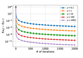
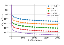
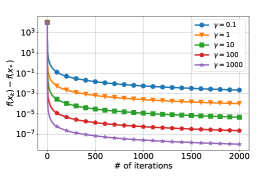
Figure 1: Convergence behavior of SPPM-inexact with different stepsizes.

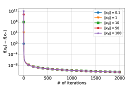
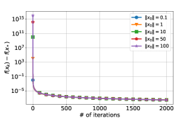
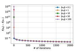
Figure 2: Convergence behavior of SPPM-inexact with different starting points.

Theorem 6.1.

Let Assumptions 2.1 (Differentiability), 2.2 (Convexity), 2.3 (Strong convexity of $f$), 2.4 (Interpolation), and 2.8 (Star Similarity) hold. If the stepsize satisfies $\gamma\leq\frac{\mu}{2\delta_{*}^{2}}$, then the iterates of SPPM satisfy, for every $k\geq 0$,

$$\mathbb{E}\big{[}\|x_{k}-x_{*}\|^{2}\big{]}\leq\left(1-\min\left(\frac{\gamma\mu}{4},\frac{1}{2}\right)\right)^{k}\|x_{0}-x_{*}\|^{2}.$$

It is worth noting that, in our result, the contraction factor is independent of the distance $\|x_{0}-x_{*}\|^{2}$ between the starting point and the solution, unlike in the case of $\phi$-smoothness. However, in this setting, the stepsize must satisfy the condition $\gamma\leq\frac{\mu}{2\delta_{*}^{2}}$.

Next, we establish convergence guarantees for SPPM-inexact. In this case, the contraction factor is not merely scaled by a constant but takes the form of the minimum of two terms. The first term, $\frac{\gamma\mu}{4}$, corresponds to the contraction factor in the exact version, differing only by a constant factor of 2. The second term, $\frac{1-c}{2}$, depends on the approximation constant $c$.

Theorem 6.2.

Let Assumptions 2.1 (Differentiability), 2.2 (Convexity), 2.4 (Interpolation) and 2.8 (Star Similarity) hold. Consider SPPM-inexact with Assumption 2.9 satsified. If the stepsize satisfies $\gamma\leq\frac{\mu}{4\delta_{*}^{2}}$ and $T$ is chosen sufficiently large such that $\frac{\eta\gamma^{2}}{T^{\alpha}}\leq c<1$, then the iterates of SPPM-inexact satisfy, for every $k\geq 0$,

$$\mathbb{E}\left[\|x_{k}-x_{*}\|^{2}\right]\leq\left(1\!-\!\min\left(\frac{\gamma\mu}{4},\frac{1\!-\!c}{2}\right)\right)^{k}\|x_{0}-x_{*}\|^{2}.$$

It is important to note that the stepsize bound depends on the strong convexity parameter $\mu$ and the similarity constant $\delta_{*}$, which are often difficult to estimate in practice due to their reliance on problem-specific properties. Despite this challenge, avoiding such a restriction seems unlikely, as these parameters are crucial to the stability and convergence of the method. Developing adaptive strategies to estimate or reduce dependence on these constants could be a valuable direction for future research.

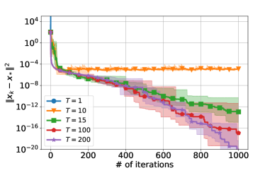
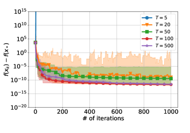
Figure 3: Convergence behavior of SPPM-inexact with different inner iterations in strongly convex and convex settings.

6.2 Non-Interpolation Regime

In this section, we derive results without assuming that all stochastic gradients vanish at the solution. In this setting, convergence is impacted by the variance, defined as follows.

Assumption 6.3 (Bounded Variance at Optimum).

Let $x_{*}$ denote any minimizer of $f$, supposed to exist. The variance of the stochastic gradients at $x_{*}$ is bounded as:

$$\mathbb{E}_{\xi\sim\mathcal{D}}\big{[}\|\nabla f_{\xi}(x_{*})\|^{2}\big{]}\leq\sigma^{2}_{*}.$$

The assumption stated above is very mild and satisfied in virtually every realistic scenario. First, we present the convergence result for the exact formulation of SPPM.

Theorem 6.4.

Let Assumptions 2.1 (Differentiability), 2.2 (Convexity), 2.3 (Strong convexity of $f$), 2.8 (Star Similarity) and 6.3 hold. If the stepsize satisfies $\gamma\leq\frac{\mu}{4\delta_{*}^{2}}$, then SPPM satisfies, for every $k\geq 0$,

$$\mathbb{E}\big{[}\|x_{k}-x_{*}\|^{2}\big{]}\leq\left(1-\frac{1}{2}\min\left(\frac{\gamma\mu}{2},1\right)\right)^{k}\|x_{0}-x_{*}\|^{2}+4\max\left(\frac{2}{\gamma\mu},1\right)\gamma^{2}\sigma_{*}^{2}.$$

The result shows linear convergence to a neighborhood of the solution, with the neighborhood size proportional to the variance $\sigma_{*}^{2}$ from Assumption 6.3, and dependent on the stepsize $\gamma$. Using a decaying stepsize schedule leads to sublinear convergence to the exact solution.

Theorem 6.5.

Let Assumptions 2.1 (Differentiability), 2.2 (Convexity), 2.8 (Star Similarity) and 6.3 (Bounded Variance) hold. Consider SPPM-inexact with Assumption 2.9 satisfied. If the stepsize satisfies $\gamma\leq\frac{\mu(1-c)}{4\delta_{*}^{2}}$ and $T$ is chosen sufficiently large such that $\frac{\eta\gamma^{2}}{T^{\alpha}}\leq c$, where $0<c<1$ is a constant, then SPPM-inexact satisfies, for every $k\geq 0$,

$$\mathbb{E}\big{[}\|x_{k}-x_{*}\|^{2}\big{]} \leq\left(1-\frac{1}{4}\min\left(\gamma\mu,1\right)\right)^{k}\|x_{0}-x_{*}\|^{2}+\max\left(\frac{1}{\gamma\mu},1\right)\frac{8\gamma^{2}\sigma_{*}^{2}}{(1-c)}.$$

The result guarantees convergence to a neighborhood of the solution, with the neighborhood size increasing by a factor of $\frac{1}{1-c}$, where $c$ is the approximation constant. Although the contraction factor remains unchanged, the stepsize must be reduced by a factor of $(1-c)$ to ensure convergence. This reduction may slow convergence compared to the exact version of SPPM, but the method remains effective as long as the approximation error is controlled.

7 Experiments

In this section, we present numerical experiments conducted for the optimization problem in the finite-sum form (2), where the functions $f_{i}$ take the specific form $f_{i}(x)=a_{i}\|x\|^{2s},$ with an integer $s\geq 2$ and $a_{i}\in\mathbb{R}^{+}$ for all $i=1,\dots,n$. Each function $f_{i}$ is $(L_{0},L_{1})$-smooth, with $L_{0}=2s$ and $L_{1}=2s-1$, and is convex. We conduct three sets of experiments to analyze the behavior of SPPM-inexact under different conditions.

The first set of experiments investigates the impact of different stepsizes on the convergence of the proposed method. Specifically, we aim to demonstrate that the method converges for any positive stepsize, provided that an appropriately chosen tolerance for the inner solver is used, and that larger stepsizes lead to faster convergence rates. To validate this, we analyze three different values of $s$, namely $s=2,3,4$. For each case, five different stepsizes are tested: $\gamma=0.1,1,10,100,1000$. The number of functions is set to $n=1000$, the dimension to $d=100$, and an inexact solver is employed with a stopping criterion based on the squared norm of the gradient, with an accuracy threshold of $10^{-12}$: $\|\nabla\Psi_{k}(\hat{x}_{k})\|^{2}\leq 10^{-12}.$ As shown in Figure 1, the method converges for all chosen stepsizes. While larger stepsizes accelerate convergence in terms of the number of iterations, they also increase the computational cost per iteration. These observations confirm our theoretical findings.

In the second set of experiments, we investigate the dependence of convergence on the initial point. The objective is to verify that the convergence of SPPM-inexact is independent of the initial point and to assess the tightness of the theoretical analysis, i.e., whether the convergence rate depends on the distance between the initial and optimal points. For this experiment, we analyze three different values of $s$ ($s=2,3,4$) and, for each case, randomly select five different initial points with norms $\|x_{0}\|=0.1,1,10,50,100$, while keeping all other parameters unchanged. As shown in Figure 2, the convergence rates are nearly identical across all cases, suggesting that the upper bound $\|x_{k}-x_{k+1}\|^{2}\leq\|x_{0}-x_{*}\|^{2}$ provided in Lemma 5.1 may be overly restrictive for certain problems. Further investigation of this effect is a promising direction for future research.

It is worth noting that increasing the parameter $s$, which influences the problem formulation, makes the problem more challenging to solve. This is because the parameters $L_{0}$ and $L_{1}$ increase as $s$ grows. This observation aligns with our theoretical understanding.

The final set of experiments investigates the effect of varying the maximum number of iterations for the inner solver, without enforcing a stopping condition based on the gradient norm. The purpose of this analysis is to demonstrate that if the inner solver fails to achieve sufficient accuracy in solving the proximal step, the method may either diverge or exhibit slower convergence. We conduct two types of experiments. In the first, we consider functions with different values of $s$, ranging from $2$ to $20$, and run the algorithm with varying maximum iteration limits for the inner solver: $T=5,20,50,100,500$. The number of functions is set to $n=100$, and the dimension is $d=5$. For the second experiment in this set, we modify the original problem to ensure strong convexity of $f$, enabling us to verify that the convergence rate becomes linear in this setting. The modified problem (2) is defined as follows: $f_{i}(x)=a_{i}\|x\|^{2s}+\lambda\langle e_{i},x\rangle^{2},$ where $a_{i}\in\mathbb{R}^{+}$ for all $i=1,\dots,n$, $\lambda\in\mathbb{R}^{+}$, and $e_{i}$ is a unit vector with its $i$-th coordinate equal to one. In this case, each function $f_{i}$ is $(L_{0},L_{1})$-smooth, with $L_{0}=2s+2\lambda$ and $L_{1}=2s-1$, and convex. Furthermore, $f$ is $\frac{\lambda}{n}$-strongly convex. We set $n=d=100$, $\lambda=2$, and $s=2$, and conduct experiments with inner solver iteration limits of $1,10,15,100,200$.

As shown in Figure 3, if the number of iterations of the subroutine is sufficiently small, the method may either diverge or exhibit significantly slower convergence. Once the number of inner iterations reaches a sufficiently large value, the convergence improves. It is worth noting that increasing the number of iterations beyond this point does not result in a significant further improvement in convergence. These observations confirm our theoretical findings.

8 Conclusion

In this work, we analyze SPPM methods under assumptions beyond standard Lipschitz smoothness. We introduce a generalized $\phi$-assumption that covers many special cases and provide convergence guarantees for both strongly convex and general settings in the interpolation regime. Additionally, we study convergence under the expected similarity assumption in strongly convex cases for both interpolation and non-interpolation regimes. Our analysis of stochastic methods beyond smoothness is a step forward in the understanding of their practical performance in ML. Further exploring SPPM in general convex settings with expected similarity is an important direction for future research.

Appendix

Appendix A Fundamental Lemmas

We define the Bregman divergence of a function $g$ as

$$D_{g}(x,y):=g(x)-g(y)-\langle\nabla g(y),x-y\rangle\quad\forall x,y\in\mathbb{R}^{d}.$$ (10)

Lemma A.1.

Let Assumptions 2.1, 2.2 and 2.4 hold. Then for any stepsize $\gamma>0$, the iterates of SPPM satisfy, for every $k\geq 0$,

$$\langle x_{k+1}-x_{*},x_{k}-x_{k+1}\rangle\geq\gamma(f_{\xi_{k}}(x_{k+1})-f_{\xi_{k}}(x_{*}))\geq 0.$$ (11)

Proof.

Since

$$x_{k+1}=\arg\min_{y\in\mathbb{R}^{d}}\left(f_{\xi_{k}}(y)+\frac{1}{2\gamma}\|y-x_{k}\|^{2}\right),$$

the first-order optimality condition implies that:

$$\nabla f_{\xi_{k}}(x_{k+1})+\frac{1}{\gamma}(x_{k+1}-x_{k})=0.$$ (12)

Since $f_{\xi_{k}}$ is differentiable and convex, we obtain the following inequality:

$$f_{\xi_{k}}(x_{*}) \geq f_{\xi_{k}}(x_{k+1})+\langle\nabla f_{\xi_{k}}(x_{k+1}),x_{*}-x_{k+1}\rangle$$

$$\overset{\eqref{eq:opt_cond}}{=}f_{\xi_{k}}(x_{k+1})+\frac{1}{\gamma}\langle x_{k}-x_{k+1},x_{*}-x_{k+1}\rangle.$$

Rearranging this expression yields the first inequality in (11). Furthermore, we also have

$$f_{\xi_{k}}(x_{k+1})\geq\inf_{x\in\mathbb{R}^{d}}f_{\xi_{k}}(x)=f_{\xi_{k}}(x_{*}),$$

which follows from Assumption 2.4. ∎

A.1 Proof of Lemma 4.2

$$f_{\xi}(x)-f_{\xi}(y) =\int_{0}^{1}\langle\nabla f_{\xi}(y+t(x-y)),x-y\rangle\,dt$$

$$=\int_{0}^{1}\langle\nabla f_{\xi}(y+t(x-y))-\nabla f_{\xi}(y),x-y\rangle\,dt+\langle\nabla f_{\xi}(y),x-y\rangle.$$

Moving $\langle\nabla f_{\xi}(y),x-y\rangle$ to the left-hand side and using Cauchy–Schwarz inequality, we get

$$D_{f_{\xi}}(x,y) =\int_{0}^{1}\langle\nabla f_{\xi}(y+t(x-y))-\nabla f_{\xi}(y),x-y\rangle\,dt$$

$$\leq\int_{0}^{1}\|\nabla f_{\xi}(y+t(x-y))-\nabla f_{\xi}(y)\|\,\|x-y\|\,dt$$

Using $\phi$-smoothness of $f_{\xi}$ and that $\phi$ is nondecreasing on both variables, we get

$$D_{f_{\xi}}(x,y) \leq\int_{0}^{1}(\phi(t\|x-y\|,\|\nabla f_{\xi}(y)\|)t\|x-y\|^{2}\,dt$$

$$\leq\int_{0}^{1}(\phi(\|x-y\|,\|\nabla f_{\xi}(y)\|)t\|x-y\|^{2}\,dt$$

$$=\frac{\phi(\|x-y\|,\|\nabla f_{\xi}(y)\|)}{2}\|x-y\|^{2}.$$ (13)

A.2 Proof of Lemma 5.1

Let $k\geq 0$. Since $x_{k+1}=\arg\min_{y\in\mathbb{R}^{d}}\left(f_{\xi_{k}}(y)+\frac{1}{2\gamma}\|y-x_{k}\|^{2}\right)$, we have

$$f_{\xi_{k}}(x_{k+1})+\frac{1}{2\gamma}\|x_{k}-x_{k+1}\|^{2}\leq f_{\xi_{k}}(x_{*})+\frac{1}{2\gamma}\|x_{k}-x_{*}\|^{2},$$

Rearranging the terms, we obtain

$$\|x_{k}-x_{k+1}\|^{2}\leq\|x_{k}-x_{*}\|^{2}-2\gamma\left(f_{\xi_{k}}(x_{k+1})-f_{\xi_{k}}(x_{*})\right).$$

Since $f_{\xi_{k}}(x_{k+1})-f_{\xi_{k}}(x_{*})\geq 0$, it follows that

$$\|x_{k}-x_{k+1}\|^{2}\leq\|x_{k}-x_{*}\|^{2}.$$

On the other hand, due to the nonexpansiveness of the proximal operator, we know that

$$\|x_{k}-x_{*}\|^{2}\leq\|x_{k-1}-x_{*}\|^{2}\quad\text{for any }k\geq 1.$$

By applying this recursively, we obtain

$$\|x_{k}-x_{*}\|^{2}\leq\|x_{0}-x_{*}\|^{2}.$$

Combining the above inequalities, we arrive at the desired result.

A.3 Proof of Lemma 5.2

Let $k\geq 0$. Applying (4.2) to the iterates, we obtain

$$f_{\xi_{k}}(x_{k})\leq f_{\xi_{k}}(x_{k+1})+\langle\nabla f_{\xi_{k}}(x_{k+1}),x_{k}-x_{k+1}\rangle+\frac{\phi\big{(}\|x_{k}-x_{k+1}\|,\|\nabla f(x_{k+1})\|\big{)}}{2}\|x_{k}-x_{k+1}\|^{2}.$$

Using (5) we obtain

$$f_{\xi_{k}}(x_{k})\leq f_{\xi_{k}}(x_{k+1})+\frac{1}{\gamma}\|x_{k}-x_{k+1}\|^{2}+\frac{\phi\left(\|x_{k}-x_{k+1}\|,\frac{1}{\gamma}\|x_{k}-x_{k+1}\|\right)}{2}\|x_{k}-x_{k+1}\|^{2}.$$

Finally, applying (5.1) and rearranging terms, we obtain

$$f_{\xi_{k}}(x_{k})-f_{\xi_{k}}(x_{k+1})\leq\left(\frac{1}{\gamma}+\frac{\phi\left(\|x_{0}-x_{*}\|,\frac{1}{\gamma}\|x_{0}-x_{*}\|\right)}{2}\right)\|x_{k}-x_{k+1}\|^{2}.$$

Appendix B Proof of Theorems 5.3 and 5.4

B.1 Proof of Theorem 5.3

For convenience, we restate Theorem 5.3 here:

Theorem B.1.

Let Assumptions 2.1 (Differentiability), 2.2 (Convexity), 2.4 (Interpolation) and 4.1 ($\phi$-smoothness) hold. Then for any stepsize $\gamma>0$ we have, for every $k\geq 0$,

$$\mathbb{E}[f(\hat{x}_{k})]-f(x_{*})\leq\frac{\phi(\|x_{0}-x_{*}\|,\frac{1}{\gamma}\|x_{0}-x_{*}\|)+\frac{2}{\gamma}}{2k}\|x_{0}-x_{*}\|^{2},$$ (14)

where $\hat{x}^{k}$ is a vector chosen from the set of iterates $x_{0}$, . . . , $x_{k-1}$ uniformly at random.

If additionally Assumption 2.3 holds, then for any stepsize $\gamma>0$ we have, for every $k\geq 0$,

$$\mathbb{E}\big{[}\|x_{k}-x_{*}\|^{2}\big{]}\leq\left(1-\frac{\mu}{\frac{2}{\gamma}+\phi(\|x_{0}-x_{*}\|,\frac{1}{\gamma}\|x_{0}-x_{*}\|)}\right)^{k}\|x_{0}-x_{*}\|^{2}.$$ (15)

Proof.

We have

$$\|x_{k+1}-x_{*}\|^{2} =\|x_{k}-x_{*}-(x_{k}-x_{k+1})\|^{2}$$

$$=\|x_{k}-x_{*}\|^{2}-2\langle x_{k}-x_{*},x_{k}-x_{k+1}\rangle+\|x_{k}-x_{k+1}\|^{2}$$

$$=\|x_{k}-x_{*}\|^{2}-2\langle x_{k}-x_{k+1}+x_{k+1}-x_{*},x_{k}-x_{k+1}\rangle+\|x_{k}-x_{k+1}\|^{2}$$

$$=\|x_{k}-x_{*}\|^{2}-2\langle x_{k+1}-x_{*},x_{k}-x_{k+1}\rangle-\|x_{k}-x_{k+1}\|^{2}.$$ (16)

Using (11) and (9), we obtain

$$\|x_{k+1}-x_{*}\|^{2}\leq\|x_{k}-x_{*}\|^{2}-2\gamma(f_{\xi_{k}}(x_{k+1})-f_{\xi_{k}}(x_{*}))-\frac{1}{\frac{1}{\gamma}+\frac{\phi\left(\|x_{0}-x_{*}\|,\frac{1}{\gamma}\|x_{0}-x_{*}\|\right)}{2}}(f_{\xi_{k}}(x_{k})-f_{\xi_{k}}(x_{k+1})).$$

Since $2\gamma>\frac{1}{\frac{1}{\gamma}+\frac{\phi\left(\|x_{0}-x_{*}\|,\frac{1}{\gamma}\|x_{0}-x_{*}\|\right)}{2}}$, we obtain

$$\|x_{k+1}-x_{*}\|^{2}\leq\|x_{k}-x_{*}\|^{2}-\frac{1}{\frac{1}{\gamma}+\frac{\phi\left(\|x_{0}-x_{*}\|,\frac{1}{\gamma}\|x_{0}-x_{*}\|\right)}{2}}(f_{\xi_{k}}(x_{k})-f_{\xi_{k}}(x_{*})).$$

Let $\mathcal{F}_{k}$ denote the $\sigma$-algebra generated by the collection of random variables $(x_{0},\ldots,x_{k})$. Taking the expectation conditioned on $\mathcal{F}_{k}$, we have

$$\mathbb{E}[\|x_{k+1}-x_{*}\|^{2}\mid\mathcal{F}_{k}]\leq\|x_{k}-x_{*}\|^{2}-\frac{1}{\frac{1}{\gamma}+\frac{\phi\left(\|x_{0}-x_{*}\|,\frac{1}{\gamma}\|x_{0}-x_{*}\|\right)}{2}}(f(x_{k})-f(x_{*})).$$ (17)

Taking full expectation, we get

$$\mathbb{E}[\|x_{k+1}-x_{*}\|^{2}]\leq\mathbb{E}[\|x_{k}-x_{*}\|^{2}]-\frac{1}{\frac{1}{\gamma}+\frac{\phi\left(\|x_{0}-x_{*}\|,\frac{1}{\gamma}\|x_{0}-x_{*}\|\right)}{2}}(\mathbb{E}[f(x_{k})]-f(x_{*})).$$

By summing up the inequalities telescopically for $t=0,\ldots,k$, we obtain

$$\sum_{t=0}^{k}\mathbb{E}[f(x_{t})]-f(x_{*}) \leq\left(\frac{1}{\gamma}+\frac{\phi\left(\|x_{0}-x_{*}\|,\frac{1}{\gamma}\|x_{0}-x_{*}\|\right)}{2}\right)(\|x_{0}-x_{*}\|^{2}-\mathbb{E}[\|x_{k+1}-x_{*}\|^{2}])$$

$$\leq\left(\frac{1}{\gamma}+\frac{\phi\left(\|x_{0}-x_{*}\|,\frac{1}{\gamma}\|x_{0}-x_{*}\|\right)}{2}\right)\|x_{0}-x_{*}\|^{2}.$$

Notice that:

$$\mathbb{E}[f(\hat{x}_{k+1})] =\mathbb{E}\left[\mathbb{E}[f(\hat{x}_{k+1})\mid\mathcal{F}_{k}]\right]=\mathbb{E}\left[\frac{1}{k+1}\sum_{t=0}^{k}f(x_{t})\right]=\frac{1}{k+1}\sum_{t=0}^{k}\mathbb{E}[f(x_{t})].$$

Thus, we have

$$\mathbb{E}[f(\hat{x}_{k+1})]-f(x_{*})\leq\frac{\frac{2}{\gamma}+\phi\left(\|x_{0}-x_{*}\|,\frac{1}{\gamma}\|x_{0}-x_{*}\|\right)}{2(k+1)}\|x_{0}-x_{*}\|^{2}.$$

If we assume 2.3, then in step (17), applying the strong convexity of $f$, we get

$$\mathbb{E}[\|x_{k+1}-x_{*}\|^{2}\mid\mathcal{F}_{k}] \leq\|x_{k}-x_{*}\|^{2}-\frac{\mu}{\frac{2}{\gamma}+\phi\left(\|x_{0}-x_{*}\|,\frac{1}{\gamma}\|x_{0}-x_{*}\|\right)}\|x_{k}-x_{*}\|^{2}$$

$$\leq\left(1-\frac{\mu}{\frac{2}{\gamma}+\phi\left(\|x_{0}-x_{*}\|,\frac{1}{\gamma}\|x_{0}-x_{*}\|\right)}\right)\|x_{k}-x_{*}\|^{2}.$$

Taking full expectation, we obtain

$$\mathbb{E}[\|x_{k+1}-x_{*}\|^{2}]\leq\left(1-\frac{\mu}{\frac{2}{\gamma}+\phi\left(\|x_{0}-x_{*}\|,\frac{1}{\gamma}\|x_{0}-x_{*}\|\right)}\right)\mathbb{E}[\|x_{k}-x_{*}\|^{2}].$$

Applying this recursively, we get

$$\mathbb{E}[\|x_{k+1}-x_{*}\|^{2}]\leq\left(1-\frac{\mu}{\frac{2}{\gamma}+\phi\left(\|x_{0}-x_{*}\|,\frac{1}{\gamma}\|x_{0}-x_{*}\|\right)}\right)^{k+1}\|x_{0}-x_{*}\|^{2}.$$

∎

B.2 Proof of Theorem 5.4

For convenience, we restate Theorem 5.4 here:

Theorem B.2.

Let Assumptions 2.1 (Differentiability), 2.2 (Convexity), 2.4 (Interpolation) and 4.1 ($\phi$-smoothness) hold. Consider SPPM-inexact with every inexact prox satisfying Assumption 2.9. If $T$ is chosen sufficiently large such that $\frac{\eta\gamma^{2}}{T^{\alpha}}\leq c<1$, then, for any stepsize $\gamma>0$ the iterates of SPPM-inexact satisfy, for every $k\geq 0$,

$$\mathbb{E}[f(\hat{x}_{k})]-f(x_{*})\leq\frac{\phi(\|x_{0}-x_{*}\|,\frac{1}{\gamma}\|x_{0}-x_{*}\|)+\frac{2}{\gamma}}{2k\left(1-c\right)}\|x_{0}-x_{*}\|^{2}.$$

If in addition Assumption 2.3 holds, then for any $\gamma>0$, the iterates of SPPM-inexact satisfy, for every $k\geq 0$,

$$\mathbb{E}\big{[}\|x_{k}-x_{*}\|^{2}\big{]}\leq\left(1-\frac{(1-c)\mu}{\frac{2}{\gamma}+\phi(\|x_{0}-x_{*}\|,\frac{1}{\gamma}\|x_{0}-x_{*}\|)}\right)^{k}\|x_{0}-x_{*}\|^{2}.$$

Proof.

We have

$$\|x_{k+1}-x_{*}\|=\|x_{k}-x_{*}\|^{2}-2\langle x_{k+1}-x_{*},x_{k}-x_{k+1}\rangle-\|x_{k}-x_{k+1}\|^{2}.$$

Substituting $x_{k+1}=x_{k}-\gamma\nabla f_{\xi_{k}}(\hat{x}_{k})$, we obtain

$$\|x_{k+1}-x_{*}\|^{2} =\|x_{k}-x_{*}\|^{2}-\|x_{k+1}-x_{k}\|^{2}-2\gamma\langle\nabla f_{\xi_{k}}(\hat{x}_{k}),x_{k+1}-x_{*}\rangle$$

$$=\|x_{k}-x_{*}\|^{2}-\|x_{k+1}-x_{k}\|^{2}-2\gamma\langle\nabla f_{\xi_{k}}(\hat{x}_{k}),x_{k+1}-\hat{x}_{k}+\hat{x}_{k}-x_{*}\rangle$$

$$=\|x_{k}-x_{*}\|^{2}-\|x_{k+1}-x_{k}\|^{2}-2\gamma\langle\nabla f_{\xi_{k}}(\hat{x}_{k}),\hat{x}_{k}-x_{*}\rangle-2\gamma\langle\nabla f_{\xi_{k}}(\hat{x}_{k}),x_{k+1}-\hat{x}_{k}\rangle.$$

Using the identity $-2\langle a,b\rangle=-\|a+b\|^{2}+\|a\|^{2}+\|b\|^{2}$, we rewrite the expression as

$$\|x_{k+1}-x_{*}\|^{2} =\|x_{k}-x_{*}\|^{2}-\|x_{k+1}-x_{k}\|^{2}-2\gamma\langle\nabla f_{\xi_{k}}(\hat{x}_{k}),\hat{x}_{k}-x_{*}\rangle$$

$$\quad-\|x_{k+1}+\gamma\nabla f_{\xi_{k}}(\hat{x}_{k})-\hat{x}_{k}\|^{2}+\|\gamma\nabla f_{\xi_{k}}(\hat{x}_{k})\|^{2}+\|x_{k+1}-\hat{x}_{k}\|^{2}.$$

Noting that $\|x_{k+1}+\gamma\nabla f_{\xi_{k}}(\hat{x}_{k})-x_{k}\|^{2}=\|x_{k}-\hat{x}_{k}\|^{2}$ and $\|\gamma\nabla f_{\xi_{k}}(\hat{x}_{k})\|^{2}=\|x_{k+1}-x_{k}\|^{2}$, we simplify as

$$\|x_{k+1}-x_{*}\|^{2} =\|x_{k}-x_{*}\|^{2}-2\gamma\langle\nabla f_{\xi_{k}}(\hat{x}_{k}),\hat{x}_{k}-x_{*}\rangle-\|x_{k}-\hat{x}_{k}\|^{2}+\|x_{k+1}-\hat{x}_{k}\|^{2}.$$

Using $\|x_{k+1}-\hat{x}_{k}\|^{2}=\|x_{k}-\gamma\nabla f_{\xi_{k}}(\hat{x}_{k})-\hat{x}_{k}\|^{2}=\|-\gamma\nabla\Psi_{k}(\hat{x}_{k})\|^{2}$, we derive

$$\|x_{k+1}-x_{*}\|^{2} =\|x_{k}-x_{*}\|^{2}-2\gamma\langle\nabla f_{\xi_{k}}(\hat{x}_{k}),\hat{x}_{k}-x_{*}\rangle-\|x_{k}-\hat{x}_{k}\|^{2}+\gamma^{2}\|\nabla\Psi_{k}(\hat{x}_{k})\|^{2}.$$ (18)

By convexity of $f_{\xi_{k}}$, we have

$$f_{\xi_{k}}(x_{*})\geq f_{\xi_{k}}(\hat{x}_{k})+\langle\nabla f_{\xi_{k}}(\hat{x}_{k}),x_{*}-\hat{x}_{k}\rangle.$$

which implies:

$$\langle\nabla f_{\xi_{k}}(\hat{x}_{k}),\hat{x}_{k}-x_{*}\rangle\geq f_{\xi_{k}}(\hat{x}_{k})-f_{\xi_{k}}(x_{*}).$$ (19)

Using (19) in (18), we get

$$\|x_{k+1}-x_{*}\|^{2}\leq\|x_{k}-x_{*}\|^{2}-2\gamma(f_{\xi_{k}}(\hat{x}_{k})-f_{\xi_{k}}(x_{*}))-\|x_{k}-\hat{x}_{k}\|^{2}+\gamma^{2}\|\nabla\Psi_{k}(\hat{x}_{k})\|^{2}.$$ (20)

Since $x_{k}^{\Psi}$ is the minimizer of $\Psi_{k}(x)$, we have

$$f_{\xi_{k}}(x_{k}^{\Psi})+\frac{1}{2\gamma}\|x_{k}^{\Psi}-x_{k}\|^{2}\leq f_{\xi_{k}}(\hat{x}_{k})+\frac{1}{2\gamma}\|\hat{x}_{k}-x_{k}\|^{2},$$

from which it follows that

$$f_{\xi_{k}}(\hat{x}_{k})\geq f_{\xi_{k}}(x_{k}^{\Psi})+\frac{1}{2\gamma}\|x_{k}^{\Psi}-x_{k}\|^{2}-\frac{1}{2\gamma}\|\hat{x}_{k}-x_{k}\|^{2}.$$

Replacing it in (20), we obtain

$$\|x_{k+1}-x_{*}\|^{2} \leq\|x_{k}-x_{*}\|^{2}-2\gamma(f_{\xi_{k}}(x_{k}^{\Psi})-f_{\xi_{k}}(x_{*}))-\|x_{k}^{\Psi}-x_{k}\|^{2}+\|\hat{x}_{k}-x_{k}\|^{2}-\|x_{k}-\hat{x}_{k}\|^{2}+\gamma^{2}\|\nabla\Psi_{k}(\hat{x}_{k})\|^{2}$$

$$=\|x_{k}-x_{*}\|^{2}-2\gamma(f_{\xi_{k}}(x_{k}^{\Psi})-f_{\xi_{k}}(x_{*}))-\|x_{k}^{\Psi}-x_{k}\|^{2}+\gamma^{2}\|\nabla\Psi_{k}(\hat{x}_{k})\|^{2}.$$ (21)

Using (2.9), we get

$$\|x_{k+1}-x_{*}\|^{2} \leq\|x_{k}-x_{*}\|^{2}-2\gamma(f_{\xi_{k}}(x_{k}^{\Psi})-f_{\xi_{k}}(x_{*}))-\|x_{k}^{\Psi}-x_{k}\|^{2}+\frac{\eta\gamma^{2}\|x_{k}-x_{k}^{\Psi}\|^{2}}{T^{\alpha}}$$

$$=\|x_{k}-x_{*}\|^{2}-2\gamma(f_{\xi_{k}}(x_{k}^{\Psi})-f_{\xi_{k}}(x_{*}))-(1-\frac{\eta\gamma^{2}}{T^{\alpha}})\|x_{k}-x_{k}^{\Psi}\|^{2}.$$ (22)

From the proximal step, we have

$$f_{\xi_{k}}(x_{k}^{\Psi})+\frac{1}{2\gamma}\|x_{k}-x_{k}^{\Psi}\|^{2}\leq f_{\xi_{k}}(x_{*})+\frac{1}{2\gamma}\|x_{*}-x_{k}\|^{2}.$$

Rearranging the terms, we get

$$\|x_{k}-x_{k}^{\Psi}\|^{2} \leq\|x_{*}-x_{k}\|^{2}-2\gamma(f_{\xi_{k}}(x_{k}^{\Psi})-f_{\xi_{k}}(x_{*}))$$

$$\leq\|x_{*}-x_{k}\|^{2},$$

and from the (22), we know that $\|x_{k+1}-x_{*}\|^{2}\leq\|x_{k}-x_{*}\|^{2}$, so using recursion, we get $\|x_{k}-x_{k}^{\Psi}\|^{2}\leq\|x_{0}-x_{*}\|^{2}$, which means we can use (9) in (22):

$$\|x_{k+1}-x_{*}\|^{2}\leq\|x_{k}-x_{*}\|^{2}-2\gamma(f_{\xi_{k}}(x_{k}^{\Psi})-f_{\xi_{k}}(x_{*}))-\frac{1-\frac{\eta\gamma^{2}}{T^{\alpha}}}{\frac{1}{\gamma}+\frac{\phi\left(\|x_{0}-x_{*}\|,\frac{1}{\gamma}\|x_{0}-x_{*}\|\right)}{2}}\left(f_{\xi_{k}}(x_{k})-f_{\xi_{k}}(x_{k}^{\Psi})\right),$$ (23)

and since $2\gamma>\frac{1-\frac{\eta\gamma^{2}}{T^{\alpha}}}{\frac{1}{\gamma}+\frac{\phi\left(\|x_{0}-x_{*}\|,\frac{1}{\gamma}\|x_{0}-x_{*}\|\right)}{2}}$, we can write

$$\|x_{k+1}-x_{*}\|^{2} \leq\|x_{k}-x_{*}\|^{2}-\frac{1-\frac{\eta\gamma^{2}}{T^{\alpha}}}{\frac{1}{\gamma}+\frac{\phi\left(\|x_{0}-x_{*}\|,\frac{1}{\gamma}\|x_{0}-x_{*}\|\right)}{2}}(f_{\xi_{k}}(x_{k}^{\Psi})-f_{\xi_{k}}(x_{*}))$$

$$\quad-\frac{1-\frac{\eta\gamma^{2}}{T^{\alpha}}}{\frac{1}{\gamma}+\frac{\phi\left(\|x_{0}-x_{*}\|,\frac{1}{\gamma}\|x_{0}-x_{*}\|\right)}{2}}\left(f_{\xi_{k}}(x_{k})-f_{\xi_{k}}(x_{k}^{\Psi})\right)$$

$$=\|x_{k}-x_{*}\|^{2}-\frac{1-\frac{\eta\gamma^{2}}{T^{\alpha}}}{\frac{1}{\gamma}+\frac{\phi\left(\|x_{0}-x_{*}\|,\frac{1}{\gamma}\|x_{0}-x_{*}\|\right)}{2}}\left(f_{\xi_{k}}(x_{k})-f_{\xi_{k}}(x_{*})\right).$$

Taking the expectation conditioned on $\mathcal{F}_{k}$, we have

$$\mathbb{E}[\|x_{k+1}-x_{*}\|^{2}\mid\mathcal{F}_{k}]\leq\|x_{k}-x_{*}\|^{2}-\frac{1-\frac{\eta\gamma^{2}}{T^{\alpha}}}{\frac{1}{\gamma}+\frac{\phi\left(\|x_{0}-x_{*}\|,\frac{1}{\gamma}\|x_{0}-x_{*}\|\right)}{2}}\left(f(x_{k})-f(x_{*})\right).$$ (24)

Now, by taking the full expectation, we get

$$\mathbb{E}[\|x_{k+1}-x_{*}\|^{2}]\leq\mathbb{E}[\|x_{k}-x_{*}\|^{2}]-\frac{1-\frac{\eta\gamma^{2}}{T^{\alpha}}}{\frac{1}{\gamma}+\frac{\phi\left(\|x_{0}-x_{*}\|,\frac{1}{\gamma}\|x_{0}-x_{*}\|\right)}{2}}\left(\mathbb{E}[f(x_{k})]-f(x_{*})\right).$$

By summing up the inequalities telescopically for $t=0,\ldots,k$, we obtain

$$\sum_{t=0}^{k}\mathbb{E}[f(x_{t})]-f(x_{*}) \leq\frac{\frac{1}{\gamma}+\frac{\phi\left(\|x_{0}-x_{*}\|,\frac{1}{\gamma}\|x_{0}-x_{*}\|\right)}{2}}{1-\frac{\eta\gamma^{2}}{T^{\alpha}}}(\|x_{0}-x_{*}\|^{2}-\mathbb{E}[\|x_{k+1}-x_{*}\|^{2}])$$

$$\leq\frac{\frac{1}{\gamma}+\frac{\phi\left(\|x_{0}-x_{*}\|,\frac{1}{\gamma}\|x_{0}-x_{*}\|\right)}{2}}{1-\frac{\eta\gamma^{2}}{T^{\alpha}}}\|x_{0}-x_{*}\|^{2}.$$

Notice that

$$\mathbb{E}[f(\hat{x}_{k+1})] =\mathbb{E}\left[\mathbb{E}[f(\hat{x}_{k+1})\mid\mathcal{F}_{k}]\right]=\mathbb{E}\left[\frac{1}{k+1}\sum_{t=0}^{k}f(x_{t})\right]=\frac{1}{k+1}\sum_{t=0}^{k}\mathbb{E}[f(x_{t})].$$

Thus, we have

$$\mathbb{E}[f(\hat{x}_{k+1})]-f(x_{*}) \leq\frac{\frac{2}{\gamma}+\phi\left(\|x_{0}-x_{*}\|,\frac{1}{\gamma}\|x_{0}-x_{*}\|\right)}{2(k+1)\left(1-\frac{\eta\gamma^{2}}{T^{\alpha}}\right)}\|x_{0}-x_{*}\|^{2}$$

$$\leq\frac{\frac{2}{\gamma}+\phi\left(\|x_{0}-x_{*}\|,\frac{1}{\gamma}\|x_{0}-x_{*}\|\right)}{2(k+1)\left(1-c\right)}\|x_{0}-x_{*}\|^{2}.$$

If we assume 2.3, then in step (24), applying the strong convexity of $f$, we get

$$\mathbb{E}[\|x_{k+1}-x_{*}\|^{2}\mid\mathcal{F}_{k}] \leq\|x_{k}-x_{*}\|^{2}-\frac{\mu\left(1-\frac{\eta\gamma^{2}}{T^{\alpha}}\right)}{\frac{2}{\gamma}+\phi\left(\|x_{0}-x_{*}\|,\frac{1}{\gamma}\|x_{0}-x_{*}\|\right)}\|x_{k}-x_{*}\|^{2}$$

$$\leq\left(1-\frac{\mu\left(1-\frac{\eta\gamma^{2}}{T^{\alpha}}\right)}{\frac{2}{\gamma}+\phi\left(\|x_{0}-x_{*}\|,\frac{1}{\gamma}\|x_{0}-x_{*}\|\right)}\right)\|x_{k}-x_{*}\|^{2}.$$

Taking the full expectation, we obtain

$$\mathbb{E}[\|x_{k+1}-x_{*}\|^{2}]\leq\left(1-\frac{\mu\left(1-\frac{\eta\gamma^{2}}{T^{\alpha}}\right)}{\frac{2}{\gamma}+\phi\left(\|x_{0}-x_{*}\|,\frac{1}{\gamma}\|x_{0}-x_{*}\|\right)}\right)\mathbb{E}[\|x_{k}-x_{*}\|^{2}].$$

Applying this recursively, we get

$$\mathbb{E}[\|x_{k+1}-x_{*}\|^{2}] \leq\left(1-\frac{\mu\left(1-\frac{\eta\gamma^{2}}{T^{\alpha}}\right)}{\frac{2}{\gamma}+\phi\left(\|x_{0}-x_{*}\|,\frac{1}{\gamma}\|x_{0}-x_{*}\|\right)}\right)^{k+1}\|x_{0}-x_{*}\|^{2}$$

$$\leq\left(1-\frac{\mu\left(1-c\right)}{\frac{2}{\gamma}+\phi\left(\|x_{0}-x_{*}\|,\frac{1}{\gamma}\|x_{0}-x_{*}\|\right)}\right)^{k+1}\|x_{0}-x_{*}\|^{2}.$$

∎

Appendix C Proof of Theorems 6.1 and 6.2

For convenience, we restate Theorem 6.1 here:

Theorem C.1.

Let Assumptions 2.1 (Differentiability), 2.2 (Convexity), 2.3(Strong convexity of $f$), 2.4 (Interpolation), and 2.8 (Star Similarity) hold. If the stepsize satisfies $\gamma\leq\frac{\mu}{2\delta_{*}^{2}}$, then we have, for every $k\geq 0$,

$$\mathbb{E}\big{[}\|x_{k}-x_{*}\|^{2}\big{]}\leq\left(1-\min\left(\frac{\gamma\mu}{4},\frac{1}{2}\right)\right)^{k}\|x_{0}-x_{*}\|^{2}.$$ (25)

Proof.

Define

$$\bar{x}_{k+1}=\mathbb{E}[x_{k+1}|\mathcal{F}_{k}].$$ (26)

Then

$$\|x_{k+1}-x_{*}\|^{2} =\|x_{k}-x_{*}\|^{2}-2\langle x_{k+1}-x_{*},x_{k}-x_{k+1}\rangle-\|x_{k}-x_{k+1}\|^{2}$$

$$\overset{\ref{eq:convexity_interpolation_ineq}}{\leq}\|x_{k}-x_{*}\|^{2}-2\gamma(f_{\xi_{k}}(x_{k+1})-f_{\xi_{k}}(x_{*}))-\|x_{k}-x_{k+1}\|^{2}$$

$$\overset{\ref{assumption:convexity}}{\leq}\|x_{k}-x_{*}\|^{2}-2\gamma(f_{\xi_{k}}(\bar{x}_{k+1})+\langle\nabla f_{\xi_{k}}(\bar{x}_{k+1}),x_{k+1}-\bar{x}_{k+1}\rangle-f_{\xi_{k}}(x_{*}))-\|x_{k}-x_{k+1}\|^{2}.$$

Taking the expectation conditioned on $\mathcal{F}_{k}$ and using the identity $\mathbb{E}[\|x-c\|^{2}]=E[\|x-\mathbb{E}[x]\|^{2}]+\|\mathbb{E}[x]-c\|^{2}$, we obtain

$$\mathbb{E}\left[\|x_{k+1}-x_{*}\|^{2}|\mathcal{F}_{k}\right] \leq\|x_{k}-x_{*}\|^{2}-2\gamma\mathbb{E}\left[f_{\xi_{k}}(\bar{x}_{k+1})+\langle\nabla f_{\xi_{k}}(\bar{x}_{k+1}),x_{k+1}-\bar{x}_{k+1}\rangle-f_{\xi_{k}}(x_{*})|\mathcal{F}_{k}\right]$$

$$\quad-\mathbb{E}\left[\|x_{k}-x_{k+1}\|^{2}|\mathcal{F}_{k}\right]$$

$$=\|x_{k}-x_{*}\|^{2}-2\gamma\left(f(\bar{x}_{k+1})-f(x_{*})+\mathbb{E}\left[\langle\nabla f_{\xi_{k}}(\bar{x}_{k+1}),x_{k+1}-\bar{x}_{k+1}\rangle|\mathcal{F}_{k}\right]\right)$$

$$\quad-\mathbb{E}\left[\|x_{k+1}-\bar{x}_{k+1}\|^{2}|\mathcal{F}_{k}\right]-\|x_{k}-\bar{x}_{k+1}\|^{2}.$$ (27)

Since $\mathbb{E}\left[\langle f(\bar{x}_{k+1}),x_{k+1}-\bar{x}_{k+1}\rangle|\mathcal{F}_{k}\right]=0$, we can write

$$\mathbb{E}\left[\|x_{k+1}-x_{*}\|^{2}|x_{k}\right] =\|x_{k}-x_{*}\|^{2}-2\gamma\left(f(\bar{x}_{k+1})-f(x_{*})+\mathbb{E}\left[\langle\nabla f_{\xi_{k}}(\bar{x}_{k+1})-\nabla f(\bar{x}_{k+1}),x_{k+1}-\bar{x}_{k+1}\rangle|x_{k}\right]\right)$$

$$\quad-\mathbb{E}\left[\|x_{k+1}-\bar{x}_{k+1}\|^{2}|x_{k}\right]-\|x_{k}-\bar{x}_{k+1}\|^{2}.$$

Using strong convexity of $f$ and the identity $2\langle a,b\rangle=\|a+b\|^{2}-\|a\|^{2}-\|b\|^{2}$, we derive

$$\mathbb{E}\left[\|x_{k+1}-x_{*}\|^{2}|\mathcal{F}_{k}\right] \leq\|x_{k}-x_{*}\|^{2}-\gamma\mu\|\bar{x}_{k+1}-x_{*}\|^{2}-\mathbb{E}\left[\|x_{k+1}-\bar{x}_{k+1}\|^{2}|\mathcal{F}_{k}\right]-\|x_{k}-\bar{x}_{k+1}\|^{2}$$

$$\quad-\mathbb{E}\Big{[}\|\gamma(\nabla f_{\xi_{k}}(\bar{x}_{k+1})-\nabla f(\bar{x}_{k+1}))+(x_{k+1}-\bar{x}_{k+1})\|^{2}-$$

$$\quad\quad\quad-\gamma^{2}\|\nabla f_{\xi_{k}}(\bar{x}_{k+1})-\nabla f(\bar{x}_{k+1})\|^{2}-\|\bar{x}_{k+1}-x_{k+1}\|^{2}\mid\mathcal{F}_{k}\Big{]}$$

$$\leq\|x_{k}-x_{*}\|^{2}-\gamma\mu\|\bar{x}_{k+1}-x_{*}\|^{2}-\|x_{k}-\bar{x}_{k+1}\|^{2}+\gamma^{2}\mathbb{E}\left[\|\nabla f_{\xi_{k}}(\bar{x}_{k+1})-\nabla f(\bar{x}_{k+1})\|^{2}|\mathcal{F}_{k}\right].$$

Finally, using the star similarity condition, we obtain

$$\mathbb{E}\left[\|x_{k+1}-x_{*}\|^{2}|\mathcal{F}_{k}\right] {\leq}\|x_{k}-x_{*}\|^{2}-\gamma\mu\|\bar{x}_{k+1}-x_{*}\|^{2}-\|x_{k}-\bar{x}_{k+1}\|^{2}+\gamma^{2}\delta_{*}^{2}\|\bar{x}_{k+1}-x_{*}\|^{2}$$

$$=\|x_{k}-x_{*}\|^{2}-(\gamma\mu-\gamma^{2}\delta_{*}^{2})\|\bar{x}_{k+1}-x_{*}\|^{2}-\|x_{k}-\bar{x}_{k+1}\|^{2}.$$

If $\gamma^{2}\delta_{*}^{2}\leq\frac{1}{2}\gamma\mu$, then $\gamma\leq\frac{\mu}{2\delta_{*}^{2}}$. Under this condition, we have

$$\mathbb{E}\left[\|x_{k+1}-x_{*}\|^{2}|\mathcal{F}_{k}\right] \leq\|x_{k}-x_{*}\|^{2}-\frac{\gamma\mu}{2}\|\bar{x}_{k+1}-x_{*}\|^{2}-\|x_{k}-\bar{x}_{k+1}\|^{2}$$

$$\leq\|x_{k}-x_{*}\|^{2}-\min\left(\frac{\gamma\mu}{2},1\right)(\|\bar{x}_{k+1}-x_{*}\|^{2}-\|x_{k}-\bar{x}_{k+1}\|^{2})$$

$$\leq\|x_{k}-x_{*}\|^{2}-\min\left(\frac{\gamma\mu}{4},\frac{1}{2}\right)\|x_{k}-x_{*}\|^{2}=\left(1-\min\left(\frac{\gamma\mu}{4},\frac{1}{2}\right)\right)\|x_{k}-x_{*}\|^{2}.$$

Taking the full expectation, we obtain

$$\mathbb{E}\left[\|x_{k+1}-x_{*}\|^{2}\right]\leq\left(1-\min\left(\frac{\gamma\mu}{4},\frac{1}{2}\right)\right)\mathbb{E}\left[\|x_{k}-x_{*}\|^{2}\right].$$

Applying this inequality recursively, we get

$$\mathbb{E}\left[\|x_{k+1}-x_{*}\|^{2}\right]\leq\left(1-\min\left(\frac{\gamma\mu}{4},\frac{1}{2}\right)\right)^{k+1}\|x_{0}-x_{*}\|^{2}.$$

∎

For convenience, we restate Theorem 6.2 here:

Theorem C.2.

Let Assumptions 2.1 (Differentiability), 2.2 (Convexity), 2.4 (Interpolation) and 2.8 (Star Similarity) hold. Consider SPPM-inexact with Assumption 2.9 satsified. If the stepsize satisfies $\gamma\leq\frac{\mu}{4\delta_{*}^{2}}$ and $T$ is chosen sufficiently large such that $\frac{\eta\gamma^{2}}{T^{\alpha}}\leq c<1$, then the iterates of SPPM-inexact satisfy, for every $k\geq 0$,

$$\mathbb{E}\left[\|x_{k}-x_{*}\|^{2}\right]\leq\left(1\!-\!\min\left(\frac{\gamma\mu}{4},\frac{1\!-\!c}{2}\right)\right)^{k}\|x_{0}-x_{*}\|^{2}.$$

Proof.

To avoid repetitions, we start from (22):

$$\|x_{k+1}-x_{*}\|\leq\|x_{k}-x_{*}\|^{2}-2\gamma(f_{\xi_{k}}(x_{k}^{\Psi})-f_{\xi_{k}}(x_{*}))-(1-\frac{\eta\gamma^{2}}{T^{\alpha}})\|x_{k}-x_{k}^{\Psi}\|^{2}.$$

Instead of (26), we define $\bar{x}_{k+1}=\mathbb{E}[x^{\Psi}_{k}|x_{k}]$.

Using convexity of $f_{\xi_{k}}$, we get

$$\|x_{k+1}-x_{*}\|\leq\|x_{k}-x_{*}\|^{2}-2\gamma(f_{\xi_{k}}(\bar{x}_{k+1})+\langle\nabla f_{\xi_{k}}(\bar{x}_{k+1}),x^{\Psi}_{k}-\bar{x}_{k+1}\rangle-f_{\xi_{k}}(x_{*}))-(1-\frac{\eta\gamma^{2}}{T^{\alpha}})\|x_{k}-x^{\Psi}_{k}\|^{2}.$$

Taking the expectation conditioned on $x_{k}$ and using the equality $\mathbb{E}[\|x-c\|^{2}]=\mathbb{E}[\|x-E[x]\|^{2}]+\|\mathbb{E}[x]-c\|^{2}$, we obtain

$$\mathbb{E}\left[\|x_{k+1}-x_{*}\|^{2}|x_{k}\right] \leq\|x_{k}-x_{*}\|^{2}-2\gamma\mathbb{E}\left[f_{\xi_{k}}(\bar{x}_{k+1})+\langle\nabla f_{\xi_{k}}(\bar{x}_{k+1}),x^{\Psi}_{k}-\bar{x}_{k+1}\rangle-f_{\xi_{k}}(x_{*})|x_{k}\right]$$

$$\quad-(1-\frac{\eta\gamma^{2}}{T^{\alpha}})E\left[\|x_{k}-x^{\Psi}_{k}\|^{2}|x_{k}\right]$$

$$=\|x_{k}-x_{*}\|^{2}-2\gamma\left(f(\bar{x}_{k+1})-f(x_{*})+\mathbb{E}\left[\langle\nabla f_{\xi_{k}}(\bar{x}_{k+1}),x^{\Psi}_{k}-\bar{x}_{k+1}\rangle|x_{k}\right]\right)$$

$$\quad-(1-\frac{\eta\gamma^{2}}{T^{\alpha}})\mathbb{E}\left[\|x^{\Psi}_{k}-\bar{x}_{k+1}\|^{2}|x_{k}\right]-(1-\frac{\eta\gamma^{2}}{T^{\alpha}})\|x_{k}-\bar{x}^{k+1}\|^{2}.$$ (28)

Since $\mathbb{E}\left[\langle f(\bar{x}_{k+1}),x_{k+1}-\bar{x}_{k+1}\rangle|x_{k}\right]=0$, we can write

$$\mathbb{E}\left[\|x_{k+1}-x_{*}\|^{2}|x_{k}\right] \leq\|x_{k}-x_{*}\|^{2}-2\gamma\left(f(\bar{x}_{k+1})-f(x_{*})+\mathbb{E}\left[\langle\nabla f_{\xi_{k}}(\bar{x}_{k+1})-f(\bar{x}_{k+1}),x^{\Psi}_{k}-\bar{x}_{k+1}\rangle|x_{k}\right]\right)$$

$$\quad-(1-\frac{\eta\gamma^{2}}{T^{\alpha}})\mathbb{E}\left[\|x^{\Psi}_{k}-\bar{x}_{k+1}\|^{2}|x_{k}\right]-(1-\frac{\eta\gamma^{2}}{T^{\alpha}})\|x_{k}-\bar{x}^{k+1}\|^{2}.$$ (29)

Let $a\in(0,1)$. Then

$$\mathbb{E}\left[\|x_{k+1}-x_{*}\|^{2}|x_{k}\right] \leq\|x_{k}-x_{*}\|^{2}-2\gamma\left(f(\bar{x}_{k+1})-f(x_{*})\right)-2\frac{1}{a}\mathbb{E}\left[\langle\gamma(\nabla f_{\xi_{k}}(\bar{x}_{k+1})-f(\bar{x}_{k+1})),a(x^{\Psi}_{k}-\bar{x}_{k+1})\rangle|x_{k}\right]$$

$$\quad-(1-\frac{\eta\gamma^{2}}{T^{\alpha}})\mathbb{E}\left[\|x^{\Psi}_{k}-\bar{x}_{k+1}\|^{2}|x_{k}\right]-(1-\frac{\eta\gamma^{2}}{T^{\alpha}})\|x_{k}-\bar{x}^{k+1}\|^{2}.$$

By applying strong convexity of $f$ and using the identity $2\langle c,b\rangle=\|c+b\|^{2}-\|c\|^{2}-\|b\|^{2}$, we have

$$\mathbb{E}\left[\|x_{k+1}-x_{*}\|^{2}|x_{k}\right] \leq\|x_{k}-x_{*}\|^{2}-\gamma\mu\|\bar{x}_{k+1}-x_{*}\|^{2}-(1-\frac{\eta\gamma^{2}}{T^{\alpha}})\mathbb{E}\left[\|x^{\Psi}_{k}-\bar{x}_{k+1}\|^{2}|x_{k}\right]-(1-\frac{\eta\gamma^{2}}{T^{\alpha}})\|x_{k}-\bar{x}_{k+1}\|^{2}$$

$$\quad-\frac{1}{a}\mathbb{E}\left[\|\gamma(\nabla f_{\xi_{k}}(\bar{x}_{k+1})-\nabla f(\bar{x}_{k+1}))+(x_{k+1}-\bar{x}_{k+1})\|^{2}|x_{k}\right]$$

$$\quad+\frac{\gamma^{2}}{a}\mathbb{E}\left[\|\nabla f_{\xi_{k}}(\bar{x}_{k+1})-\nabla f(\bar{x}_{k+1})\|^{2}|x_{k}\right]+a\mathbb{E}\left[\|\bar{x}_{k+1}-x^{\Psi}_{k}\|^{2}|x_{k}\right].$$

By setting $a=(1-\frac{\eta\gamma^{2}}{T^{\alpha}})$, we obtain

$$\mathbb{E}\left[\|x_{k+1}-x_{*}\|^{2}|x_{k}\right] \leq\|x_{k}-x_{*}\|^{2}-\gamma\mu\|\bar{x}_{k+1}-x_{*}\|^{2}-(1-\frac{\eta\gamma^{2}}{T^{\alpha}})\|x_{k}-\bar{x}_{k+1}\|^{2}$$

$$\quad+\frac{\gamma^{2}}{(1-\frac{\eta\gamma^{2}}{T^{\alpha}})}\mathbb{E}\left[\|\nabla f_{\xi_{k}}(\bar{x}_{k+1})-\nabla f(\bar{x}_{k+1})\|^{2}|x_{k}\right].$$

Now, using the star similarity assumption (2.8), we get

$$\mathbb{E}\left[\|x_{k+1}-x_{*}\|^{2}|x_{k}\right] \leq\|x_{k}-x_{*}\|^{2}-\gamma\mu\|\bar{x}_{k+1}-x_{*}\|^{2}-(1-\frac{\eta\gamma^{2}}{T^{\alpha}})\|x_{k}-\bar{x}_{k+1}\|^{2}+\frac{\gamma^{2}\delta_{*}^{2}}{(1-\frac{\eta\gamma^{2}}{T^{\alpha}})}\|\bar{x}_{k+1}-x_{*}\|^{2}.$$

Assuming $T$ sufficiently large such that $\frac{\eta\gamma^{2}}{T^{\alpha}}\leq c<1$, we obtain

$$\mathbb{E}\left[\|x_{k+1}-x_{*}\|^{2}|x_{k}\right] \leq\|x_{k}-x_{*}\|^{2}-\gamma\mu\|\bar{x}_{k+1}-x_{*}\|^{2}-(1-c)\|x_{k}-\bar{x}_{k+1}\|^{2}+2\gamma^{2}\delta_{*}^{2}\|\bar{x}_{k+1}-x_{*}\|^{2}.$$

We want $2\gamma^{2}\delta_{*}^{2}\leq\frac{\gamma\mu}{2}$, which means $\gamma\leq\frac{\mu}{4\delta_{*}^{2}}$, so we get

$$\mathbb{E}\left[\|x_{k+1}-x_{*}\|^{2}|x_{k}\right] \leq\|x_{k}-x_{*}\|^{2}-\min\left(\frac{\gamma\mu}{2},1-c\right)(\|\bar{x}_{k+1}-x_{*}\|^{2}-\|x_{k}-\bar{x}_{k+1}\|^{2})$$

$$\leq\|x_{k}-x_{*}\|^{2}-\min\left(\frac{\gamma\mu}{4},\frac{1-c}{2}\right)\|x_{k}-x_{*}\|^{2}$$

$$=\left(1-\min\left(\frac{\gamma\mu}{4},\frac{1-c}{2}\right)\right)\|x_{k}-x_{*}\|^{2}.$$

Taking the full expectation, we obtain

$$\mathbb{E}\left[\|x_{k+1}-x_{*}\|^{2}\right]\leq\left(1-\min\left(\frac{\gamma\mu}{4},\frac{1-c}{2}\right)\right)\mathbb{E}\left[\|x_{k}-x_{*}\|^{2}\right].$$

Iterating over $k$, the result follows:

$$\mathbb{E}\big{[}\|x_{k+1}-x_{*}\|^{2}\big{]}\leq\left(1-\min\left(\frac{\gamma\mu}{4},\frac{1-c}{2}\right)\right)^{k+1}\|x_{0}-x_{*}\|^{2}.$$

∎

Appendix D Proof of Theorems 6.4 and 6.5

For convenience, we restate Theorem 6.4 here:

Theorem D.1.

Let Assumptions 2.1 (Differentiability), 2.2 (Convexity), 2.3(Strong convexity of $f$), 2.8 (Star Similarity) and 6.3 (Bounded Variance at Optimum) hold. If the stepsize satisfies $\gamma\leq\frac{\mu}{4\delta_{*}^{2}}$, we have, for every $k\geq 0$,

$$\mathbb{E}\big{[}\|x_{k}-x_{*}\|^{2}\big{]}\leq\left(1-\min\left(\frac{\gamma\mu}{4},\frac{1}{2}\right)\right)^{k}\|x_{0}-x_{*}\|^{2}+\max\left(\frac{4}{\gamma\mu},2\right)2\gamma^{2}\sigma_{*}^{2}.$$ (30)

Proof.

Define

$$\bar{x}_{k+1}=\mathbb{E}[x_{k+1}|\mathcal{F}_{k}].$$

Then

$$\|x_{k+1}-x_{*}\|^{2} =\|x_{k}-x_{*}\|^{2}-2\langle x_{k+1}-x_{*},x_{k}-x_{k+1}\rangle-\|x_{k}-x_{k+1}\|^{2}$$

$$\leq\|x_{k}-x_{*}\|^{2}-2\gamma(f_{\xi_{k}}(x_{k+1})-f_{\xi_{k}}(x_{*}))-\|x_{k}-x_{k+1}\|^{2}$$

$$\leq\|x_{k}-x_{*}\|^{2}-2\gamma(f_{\xi_{k}}(\bar{x}_{k+1})+\langle\nabla f_{\xi_{k}}(\bar{x}_{k+1}),x_{k+1}-\bar{x}_{k+1}\rangle-f_{\xi_{k}}(x_{*}))-\|x_{k}-x_{k+1}\|^{2}.$$

Taking the expectation conditioned on $\mathcal{F}_{k}$ and using the equality $\mathbb{E}[\|x-c\|^{2}]=\mathbb{E}[\|x-\mathbb{E}[x]\|^{2}]+\|\mathbb{E}[x]-c\|^{2}$, we get

$$\mathbb{E}\left[\|x_{k+1}-x_{*}\|^{2}|\mathcal{F}_{k}\right] \leq\|x_{k}-x_{*}\|^{2}-2\gamma\mathbb{E}\left[f_{\xi_{k}}(\bar{x}_{k+1})+\langle\nabla f_{\xi_{k}}(\bar{x}_{k+1}),x_{k+1}-\bar{x}_{k+1}\rangle-f_{\xi_{k}}(x_{*})|\mathcal{F}_{k}\right]$$

$$\quad-\mathbb{E}\left[\|x_{k}-x_{k+1}\|^{2}|\mathcal{F}_{k}\right]$$

$$=\|x_{k}-x_{*}\|^{2}-2\gamma\left(f(\bar{x}_{k+1})-f(x_{*})+\mathbb{E}\left[\langle\nabla f_{\xi_{k}}(\bar{x}_{k+1}),x_{k+1}-\bar{x}_{k+1}\rangle|\mathcal{F}_{k}\right]\right)$$

$$\quad-\mathbb{E}\left[\|x_{k+1}-\bar{x}_{k+1}\|^{2}|x_{k}\right]-\|x_{k}-\bar{x}_{k+1}\|^{2}.$$ (31)

Since $\mathbb{E}\left[\langle f(\bar{x}_{k+1}),x_{k+1}-\bar{x}_{k+1}\rangle|\mathcal{F}_{k}\right]=0$, we can write:

$$\mathbb{E}\left[\|x_{k+1}-x_{*}\|^{2}\mid\mathcal{F}_{k}\right] \leq\|x_{k}-x_{*}\|^{2}-2\gamma\left(f(\bar{x}_{k+1})-f(x_{*})+\mathbb{E}\left[\langle\nabla f_{\xi_{k}}(\bar{x}_{k+1}),x_{k+1}-\bar{x}_{k+1}\rangle\mid\mathcal{F}_{k}\right]\right)$$

$$\quad-\mathbb{E}\left[\|x_{k+1}-\bar{x}_{k+1}\|^{2}\mid\mathcal{F}_{k}\right]-\|x_{k}-\bar{x}_{k+1}\|^{2}$$

$$=\|x_{k}-x_{*}\|^{2}-2\gamma\left(f(\bar{x}_{k+1})-f(x_{*})\right)$$

$$\quad-2\gamma\mathbb{E}\left[\langle\nabla f_{\xi_{k}}(\bar{x}_{k+1})-\nabla f(\bar{x}_{k+1})-\nabla f_{\xi_{k}}(x_{*}),x_{k+1}-\bar{x}_{k+1}\rangle\mid\mathcal{F}_{k}\right]$$

$$\quad+2\gamma\left(\mathbb{E}\left[\langle\nabla f_{\xi_{k}}(x_{*}),\bar{x}_{k+1}-x_{k+1}\rangle\mid\mathcal{F}_{k}\right]\right)-\mathbb{E}\left[\|x_{k+1}-\bar{x}_{k+1}\|^{2}\mid\mathcal{F}_{k}\right]-\|x_{k}-\bar{x}_{k+1}\|^{2}.$$

Let $a\in(0,1)$. Then

$$\mathbb{E}\left[\|x_{k+1}-x_{*}\|^{2}\mid\mathcal{F}_{k}\right] \leq\|x_{k}-x_{*}\|^{2}-2\gamma\left(f(\bar{x}_{k+1})-f(x_{*})\right)$$

$$\quad-\frac{2}{a}E\left[\langle\gamma(\nabla f_{\xi_{k}}(\bar{x}_{k+1})-\nabla f(\bar{x}_{k+1})-\nabla f_{\xi_{k}}(x_{*})),a(x_{k+1}-\bar{x}_{k+1})\rangle\mid\mathcal{F}_{k}\right]$$

$$\quad+2\gamma\left(\mathbb{E}\left[\langle\nabla f_{\xi_{k}}(x_{*}),\bar{x}_{k+1}-x_{k+1}\rangle\mid\mathcal{F}_{k}\right]\right)-\mathbb{E}\left[\|x_{k+1}-\bar{x}_{k+1}\|^{2}\mid\mathcal{F}_{k}\right]-\|x_{k}-\bar{x}_{k+1}\|^{2}.$$

Using strong convexity of $f$ and the identity $2\langle c,b\rangle=\|c+b\|^{2}-\|c\|^{2}-\|b\|^{2}$, we obtain

$$\mathbb{E}\left[\|x_{k+1}-x_{*}\|^{2}\right] \leq\|x_{k}-x_{*}\|^{2}-\gamma\mu\|\bar{x}_{k+1}-x_{*}\|^{2}$$

$$\quad-\frac{1}{a}\mathbb{E}\left[\|\gamma(\nabla f_{\xi_{k}}(\bar{x}_{k+1})-\nabla f(\bar{x}_{k+1})-\nabla f_{\xi_{k}}(x_{*}))+a(x_{k+1}-\bar{x}_{k+1})\|^{2}\mid\mathcal{F}_{k}\right]$$

$$\quad+\frac{\gamma^{2}}{a}\mathbb{E}\left[\|(\nabla f_{\xi_{k}}(\bar{x}_{k+1})-\nabla f(\bar{x}_{k+1})-\nabla f_{\xi_{k}}(x_{*}))\|^{2}\mid\mathcal{F}_{k}\right]-(1-a)\mathbb{E}\left[\|x_{k+1}-\bar{x}_{k+1}\|^{2}\mid\mathcal{F}_{k}\right]$$

$$\quad+2\gamma\left(\mathbb{E}\left[\langle\nabla f_{\xi_{k}}(x_{*}),\bar{x}_{k+1}-x_{k+1}\rangle\mid\mathcal{F}_{k}\right]\right)-\|x_{k}-\bar{x}_{k+1}\|^{2}.$$

Using Assumption 2.8 and Young’s inequality, we get

$$\mathbb{E}\left[\|x_{k+1}-x_{*}\|^{2}\right] \leq\|x_{k}-x_{*}\|^{2}-\gamma\mu\|\bar{x}_{k+1}-x_{*}\|^{2}+\frac{\gamma^{2}\delta_{*}^{2}}{a}\|\bar{x}_{k+1}-x_{*}\|^{2}-(1-a)\mathbb{E}\left[\|x_{k+1}-\bar{x}_{k+1}\|^{2}\mid x_{k}\right]$$

$$\quad+\frac{\gamma^{2}}{s}\mathbb{E}\left[\|\nabla f_{\xi_{k}}(x_{*})\|^{2}\mid x_{k}\right]+s\mathbb{E}\left[\|x_{k+1}-\bar{x}_{k+1}\|^{2}\mid x_{k}\right]-\|x_{k}-\bar{x}_{k+1}\|^{2}.$$

By substituting $s=1-a$ and choosing $a=\frac{1}{2}$, we get

$$\mathbb{E}\left[\|x_{k+1}-x_{*}\|^{2}\mathcal{F}_{k}\right] \leq\|x_{k}-x_{*}\|^{2}-\gamma\mu\|\bar{x}_{k+1}-x_{*}\|^{2}+2\gamma^{2}\delta_{*}^{2}\|\bar{x}_{k+1}-x_{*}\|^{2}+2\gamma^{2}\mathbb{E}\left[\|\nabla f_{\xi_{k}}(x_{*})\|^{2}\mid x_{k}\right]$$

$$\quad-\|x_{k}-\bar{x}_{k+1}\|^{2}.$$

We require $2\gamma^{2}\delta_{*}^{2}\leq\frac{\gamma\mu}{2}$, which implies $\gamma\leq\frac{\mu}{4\delta_{*}^{2}}$. Therefore, we get

$$\mathbb{E}\left[\|x_{k+1}-x_{*}\|^{2}\mid\mathcal{F}_{k}\right] \leq\|x_{k}-x_{*}\|^{2}-\frac{\gamma\mu}{2}\|\bar{x}_{k+1}-x_{*}\|^{2}-\|x_{k}-\bar{x}_{k+1}\|^{2}+2\gamma^{2}\mathbb{E}\left[\|\nabla f_{\xi_{k}}(x_{*})\|^{2}\mid x_{k}\right]$$

$$\leq\|x_{k}-x_{*}\|^{2}-\min\left(\frac{\gamma\mu}{2},1\right)(\|\bar{x}_{k+1}-x_{*}\|^{2}-\|x_{k}-\bar{x}_{k+1}\|^{2})+2\gamma^{2}\mathbb{E}\left[\|\nabla f_{\xi_{k}}(x_{*})\|^{2}\mid x_{k}\right]$$

$$\leq\left(1-\min\left(\frac{\gamma\mu}{4},\frac{1}{2}\right)\right)\|x_{k}-x_{*}\|^{2}+2\gamma^{2}\sigma_{*}^{2}.$$

Taking the full expectation, we obtain

$$\mathbb{E}[\|x_{k+1}-x_{*}\|^{2}]\leq\left(1-\min\left(\frac{\gamma\mu}{4},\frac{1}{2}\right)\right)\mathbb{E}[\|x_{k}-x_{*}\|^{2}]+2\gamma^{2}\sigma_{*}^{2}.$$

By applying the inequality recursively, we derive

$$\mathbb{E}[\|x_{k+1}-x_{*}\|^{2}] \leq\left(1-\min\left(\frac{\gamma\mu}{4},\frac{1}{2}\right)\right)^{k+1}\|x_{0}-x_{*}\|^{2}$$

$$\quad+\left(\left(1-\min\left(\frac{\gamma\mu}{4},\frac{1}{2}\right)\right)^{0}+\dots+\left(1-\min\left(\frac{\gamma\mu}{4},\frac{1}{2}\right)\right)^{k}\right)2\gamma^{2}\sigma_{*}^{2}$$

$$\leq\left(1-\min\left(\frac{\gamma\mu}{4},\frac{1}{2}\right)\right)^{k+1}\|x_{0}-x_{*}\|^{2}+\max\left(\frac{4}{\gamma\mu},2\right)2\gamma^{2}\sigma_{*}^{2}.$$

∎

For convenience, we restate Theorem 6.5 here:

Theorem D.2.

Let Assumptions 2.1 (Differentiability), 2.2 (Convexity), 2.8 (Star Similarity) and 6.3 (Bounded Variance) hold. Consider SPPM-inexact with Assumption 2.9 satisfied. If the stepsize satisfies $\gamma\leq\frac{\mu(1-c)}{4\delta_{*}^{2}}$ and $T$ is chosen sufficiently large such that $\frac{\eta\gamma^{2}}{T^{\alpha}}\leq c$, where $0<c<1$ is a constant, then SPPM-inexact satisfies, for every $k\geq 0$,

$$\mathbb{E}\big{[}\|x_{k}-x_{*}\|^{2}\big{]}\leq\left(1-\frac{1}{4}\min\left(\gamma\mu,1\right)\right)^{k}\|x_{0}-x_{*}\|^{2}+\max\left(\frac{1}{\gamma\mu},1\right)\frac{8\gamma^{2}\sigma_{*}^{2}}{(1-c)}.$$

Proof.

To avoid repetition, we start from (28):

$$\mathbb{E}\left[\|x_{k+1}-x_{*}\|^{2}|x_{k}\right] \leq\|x_{k}-x_{*}\|^{2}-2\gamma\left(f(\bar{x}_{k+1})-f(x_{*})+\mathbb{E}\left[\langle\nabla f_{\xi_{k}}(\bar{x}_{k+1}),x^{\Psi}_{k}-\bar{x}_{k+1}\rangle|x_{k}\right]\right)$$

$$\quad-(1-\frac{\eta\gamma^{2}}{T^{\alpha}})\mathbb{E}\left[\|x^{\Psi}_{k}-\bar{x}_{k+1}\|^{2}|x_{k}\right]-(1-\frac{\eta\gamma^{2}}{T^{\alpha}})\|x_{k}-\bar{x}^{k+1}\|^{2}.$$

Now since $\mathbb{E}\left[\langle f(\bar{x}_{k+1}),x^{\Psi}_{k}-\bar{x}_{k+1}\rangle|x_{k}\right]=0$, we can write

$$\mathbb{E}\left[\|x_{k+1}-x_{*}\|^{2}\mid x_{k}\right] \leq\|x_{k}-x_{*}\|^{2}-2\gamma\left(f(\bar{x}_{k+1})-f(x_{*})\right)$$

$$\quad-2\gamma\mathbb{E}\left[\langle\nabla f_{\xi_{k}}(\bar{x}_{k+1})-\nabla f(\bar{x}_{k+1})-\nabla f_{\xi_{k}}(x_{*}),x^{\Psi}_{k}-\bar{x}_{k+1}\rangle\mid x_{k}\right]$$

$$\quad+2\gamma\left(\mathbb{E}\left[\langle\nabla f_{\xi_{k}}(x_{*}),\bar{x}_{k+1}-x^{\Psi}_{k}\rangle\mid x_{k}\right]\right)-(1-\frac{\eta\gamma^{2}}{T^{\alpha}})\mathbb{E}\left[\|x^{\Psi}_{k}-\bar{x}_{k+1}\|^{2}\mid x_{k}\right]$$

$$\quad-\left(1-\frac{\eta\gamma^{2}}{T^{\alpha}}\right)\|x_{k}-\bar{x}_{k+1}\|^{2}.$$

Let $a\in(0,1)$. Then

$$\mathbb{E}\left[\|x_{k+1}-x_{*}\|^{2}\mid x_{k}\right] \leq\|x_{k}-x_{*}\|^{2}-2\gamma\left(f(\bar{x}_{k+1})-f(x_{*})\right)$$

$$\quad-2\frac{1}{a}\left(\mathbb{E}\left[\langle\gamma(\nabla f_{\xi_{k}}(\bar{x}_{k+1})-\nabla f(\bar{x}_{k+1})-\nabla f_{\xi_{k}}(x_{*})),a(x^{\Psi}_{k}-\bar{x}_{k+1})\rangle\mid x_{k}\right]\right)$$

$$\quad+2\gamma\left(\mathbb{E}\left[\langle\nabla f_{\xi_{k}}(x_{*}),\bar{x}_{k+1}-x^{\Psi}_{k}\rangle\mid x_{k}\right]\right)-(1-\frac{\eta\gamma^{2}}{T^{\alpha}})\mathbb{E}\left[\|x^{\Psi}_{k}-\bar{x}_{k+1}\|^{2}\mid x_{k}\right]$$

$$\quad-\left(1-\frac{\eta\gamma^{2}}{T^{\alpha}}\right)\|x_{k}-\bar{x}_{k+1}\|^{2}.$$

Using strong convexity of $f$ and the identity $2\langle c,b\rangle=\|c+b\|^{2}-\|c\|^{2}-\|b\|^{2}$, we obtain

$$\mathbb{E}\left[\|x_{k+1}-x_{*}\|^{2}\mid x_{k}\right] \leq\|x_{k}-x_{*}\|^{2}-\gamma\mu\|\bar{x}_{k+1}-x_{*}\|^{2}$$

$$\quad-\frac{1}{a}\left(\mathbb{E}\left[\|\gamma(\nabla f_{\xi_{k}}(\bar{x}_{k+1})-\nabla f(\bar{x}_{k+1})-\nabla f_{\xi_{k}}(x_{*}))+a(x^{\Psi}_{k}-\bar{x}_{k+1})\|^{2}\mid x_{k}\right]\right)$$

$$\quad+\frac{\gamma^{2}}{a}\mathbb{E}\left[\|(\nabla f_{\xi_{k}}(\bar{x}_{k+1})-\nabla f(\bar{x}_{k+1})-\nabla f_{\xi_{k}}(x_{*}))\|^{2}\mid x_{k}\right]+a\mathbb{E}\left[\|x^{\Psi}_{k}-\bar{x}_{k+1}\|^{2}\mid x_{k}\right]$$

$$\quad+2\gamma\left(\mathbb{E}\left[\langle\nabla f_{\xi_{k}}(x_{*}),\bar{x}_{k+1}-x^{\Psi}_{k}\rangle\mid x_{k}\right]\right)-(1-\frac{\eta\gamma^{2}}{T^{\alpha}})\mathbb{E}\left[\|x^{\Psi}_{k}-\bar{x}_{k+1}\|^{2}\mid x_{k}\right]$$

$$\quad-\left(1-\frac{\eta\gamma^{2}}{T^{\alpha}}\right)\|x_{k}-\bar{x}_{k+1}\|^{2}.$$

Using Assumption 2.8 and Young’s inequality, we get

$$\mathbb{E}\left[\|x_{k+1}-x_{*}\|^{2}\mid x_{k}\right] \leq\|x_{k}-x_{*}\|^{2}-\gamma\mu\|\bar{x}_{k+1}-x_{*}\|^{2}+\frac{\gamma^{2}\delta_{*}^{2}}{a}\|\bar{x}_{k+1}-x_{*}\|^{2}+a\mathbb{E}\left[\|x^{\Psi}_{k}-\bar{x}_{k+1}\|^{2}\mid x_{k}\right]$$

$$\quad+\frac{\gamma^{2}}{s}\mathbb{E}\left[\|\nabla f_{\xi_{k}}(x_{*})\|^{2}\mid x_{k}\right]+sE\left[\|\bar{x}_{k+1}-x^{\Psi}_{k}\|^{2}\mid x_{k}\right]-(1-\frac{\eta\gamma^{2}}{T^{\alpha}})\mathbb{E}\left[\|x^{\Psi}_{k}-\bar{x}_{k+1}\|^{2}\mid x_{k}\right]$$

$$\quad-\left(1-\frac{\eta\gamma^{2}}{T^{\alpha}}\right)\|x_{k}-\bar{x}_{k+1}\|^{2}.$$

Choosing $s=a=\frac{1-\frac{\eta\gamma^{2}}{T^{\alpha}}}{2}$, we derive

$$\mathbb{E}\left[\|x_{k+1}-x_{*}\|^{2}\mid x_{k}\right] \leq\|x_{k}-x_{*}\|^{2}-\gamma\mu\|\bar{x}_{k+1}-x_{*}\|^{2}+\frac{2\gamma^{2}\delta_{*}^{2}}{1-\frac{\eta\gamma^{2}}{T^{\alpha}}}\|\bar{x}_{k+1}-x_{*}\|^{2}+\frac{2\gamma^{2}}{1-\frac{\eta\gamma^{2}}{T^{\alpha}}}\mathbb{E}\left[\|\nabla f_{\xi_{k}}(x_{*})\|^{2}\mid x_{k}\right]$$

$$\quad-\left(1-\frac{\eta\gamma^{2}}{T^{\alpha}}\right)\|x_{k}-\bar{x}_{k+1}\|^{2}.$$

Let $T$ be large enough such that $\frac{\eta\gamma^{2}}{T^{\alpha}}\leq c<1$. Then

$$\mathbb{E}\left[\|x_{k+1}-x_{*}\|^{2}\mid x_{k}\right] \leq\|x_{k}-x_{*}\|^{2}-\gamma\mu\|\bar{x}_{k+1}-x_{*}\|^{2}+\frac{2\gamma^{2}\delta_{*}^{2}}{1-c}\|\bar{x}_{k+1}-x_{*}\|^{2}+\frac{2\gamma^{2}}{1-c}\mathbb{E}\left[\|\nabla f_{\xi_{k}}(x_{*})\|^{2}\mid x_{k}\right]$$

$$\quad-(1-c)\|x_{k}-\bar{x}_{k+1}\|^{2}.$$

We want $2\gamma^{2}\delta_{*}^{2}\leq\frac{\gamma\mu(1-c)}{2}$, which implies $\gamma\leq\frac{\mu(1-c)}{4\delta_{*}^{2}}$, so we get

$$\mathbb{E}\left[\|x_{k+1}-x_{*}\|^{2}\mid x_{k}\right] \leq\|x_{k}-x_{*}\|^{2}-\frac{\gamma\mu}{2}\|\bar{x}_{k+1}-x_{*}\|^{2}-\frac{1}{2}\|x_{k}-\bar{x}_{k+1}\|^{2}+\frac{2\gamma^{2}}{1-c}\mathbb{E}\left[\|\nabla f_{\xi_{k}}(x_{*})\|^{2}\mid x_{k}\right]$$

$$\leq\|x_{k}-x_{*}\|^{2}-\min\left(\frac{\gamma\mu}{4},\frac{1}{4}\right)\|x_{k}-\bar{x}_{*}\|^{2}+\frac{2\gamma^{2}}{1-c}\mathbb{E}\left[\|\nabla f_{\xi_{k}}(x_{*})\|^{2}\mid x_{k}\right]$$

$$\overset{\ref{assumption:bounded_variance}}{\leq}\left(1-\min\left(\frac{\gamma\mu}{4},\frac{1}{4}\right)\right)\|x_{k}-x_{*}\|^{2}+\frac{2\gamma^{2}\sigma_{*}^{2}}{1-c}.$$

Taking the full expectation, we obtain

$$\mathbb{E}\left[\|x_{k+1}-x_{*}\|^{2}\right]\leq\left(1-\min\left(\frac{\gamma\mu}{4},\frac{1}{4}\right)\right)\mathbb{E}[\|x_{k}-x_{*}\|^{2}]+\frac{2\gamma^{2}\sigma_{*}^{2}}{1-c}.$$

By applying the inequality recursively, we derive

$$\mathbb{E}[\|x_{k+1}-x_{*}\|^{2}] \leq\left(1-\min\left(\frac{\gamma\mu}{4},\frac{1}{4}\right)\right)^{k+1}\|x_{0}-x_{*}\|^{2}$$

$$\quad+\left(\left(1-\min\left(\frac{\gamma\mu}{4},\frac{1}{4}\right)\right)^{0}+\dots+\left(1-\min\left(\frac{\gamma\mu}{4},\frac{1}{4}\right)\right)^{k}\right)\frac{2\gamma^{2}\sigma_{*}^{2}}{1-c}$$

$$\leq\left(1-\frac{1}{4}\min\left(\gamma\mu,1\right)\right)^{k+1}\|x_{0}-x_{*}\|^{2}+\max\left(\frac{1}{\gamma\mu},1\right)\frac{8\gamma^{2}\sigma_{*}^{2}}{(1-c)}.$$

∎

References

- Agarwal & Bottou (2015) Agarwal, A. and Bottou, L. A lower bound for the optimization of finite sums. In International conference on machine learning, pp. 78–86. PMLR, 2015.
- Asi & Duchi (2019) Asi, H. and Duchi, J. C. Stochastic (approximate) proximal point methods: Convergence, optimality, and adaptivity. SIAM Journal on Optimization, 29(3):2257–2290, 2019.
- Asi et al. (2020) Asi, H., Chadha, K., Cheng, G., and Duchi, J. C. Minibatch stochastic approximate proximal point methods. Advances in neural information processing systems, 33:21958–21968, 2020.
- Bauschke et al. (2017) Bauschke, H. H., Combettes, P. L., Bauschke, H. H., and Combettes, P. L. Correction to: convex analysis and monotone operator theory in Hilbert spaces. Springer, 2017.
- Bertsekas (2011) Bertsekas, D. P. Incremental proximal methods for large scale convex optimization. Mathematical programming, 129(2):163–195, 2011.
- Bianchi (2016) Bianchi, P. Ergodic convergence of a stochastic proximal point algorithm. SIAM Journal on Optimization, 26(4):2235–2260, 2016.
- Borodich et al. (2023) Borodich, E., Kormakov, G., Kovalev, D., Beznosikov, A., and Gasnikov, A. Optimal algorithm with complexity separation for strongly convex-strongly concave composite saddle point problems. arXiv preprint arXiv:2307.12946, 2023.
- Bottou et al. (2018) Bottou, L., Curtis, F. E., and Nocedal, J. Optimization methods for large-scale machine learning. SIAM review, 60(2):223–311, 2018.
- Cai et al. (2023) Cai, X., Song, C., Wright, S., and Diakonikolas, J. Cyclic block coordinate descent with variance reduction for composite nonconvex optimization. In International Conference on Machine Learning, pp. 3469–3494. PMLR, 2023.
- Carratino et al. (2018) Carratino, L., Rudi, A., and Rosasco, L. Learning with sgd and random features. Advances in neural information processing systems, 31, 2018.
- Chen et al. (2023) Chen, Z., Zhou, Y., Liang, Y., and Lu, Z. Generalized-smooth nonconvex optimization is as efficient as smooth nonconvex optimization. In International Conference on Machine Learning, pp. 5396–5427. PMLR, 2023.
- Condat & Richtárik (2022) Condat, L. and Richtárik, P. Randprox: Primal-dual optimization algorithms with randomized proximal updates. arXiv preprint arXiv:2207.12891, 2022.
- Condat & Richtárik (2024) Condat, L. and Richtárik, P. A simple linear convergence analysis of the point-saga algorithm. arXiv preprint arXiv:2405.19951, 2024.
- Condat et al. (2022) Condat, L., Malinovsky, G., and Richtárik, P. Distributed proximal splitting algorithms with rates and acceleration. Frontiers in Signal Processing, 1:776825, 2022.
- Condat et al. (2023a) Condat, L., Agarskỳ, I., Malinovsky, G., and Richtárik, P. Tamuna: Doubly accelerated federated learning with local training, compression, and partial participation. In International Workshop on Federated Learning in the Age of Foundation Models in Conjunction with NeurIPS 2023, 2023a.
- Condat et al. (2023b) Condat, L., Kitahara, D., Contreras, A., and Hirabayashi, A. Proximal splitting algorithms for convex optimization: A tour of recent advances, with new twists. SIAM Review, 65(2):375–435, 2023b.
- Crawshaw et al. (2022) Crawshaw, M., Liu, M., Orabona, F., Zhang, W., and Zhuang, Z. Robustness to unbounded smoothness of generalized signsgd. Advances in neural information processing systems, 35:9955–9968, 2022.
- Crawshaw et al. (2024) Crawshaw, M., Bao, Y., and Liu, M. Federated learning with client subsampling, data heterogeneity, and unbounded smoothness: A new algorithm and lower bounds. Advances in Neural Information Processing Systems, 36, 2024.
- Davis & Drusvyatskiy (2019) Davis, D. and Drusvyatskiy, D. Stochastic model-based minimization of weakly convex functions. SIAM Journal on Optimization, 29(1):207–239, 2019.
- Davis & Yin (2017) Davis, D. and Yin, W. A three-operator splitting scheme and its optimization applications. Set-valued and variational analysis, 25:829–858, 2017.
- Defazio & Bottou (2019) Defazio, A. and Bottou, L. On the ineffectiveness of variance reduced optimization for deep learning. Advances in Neural Information Processing Systems, 32, 2019.
- Defazio et al. (2014) Defazio, A., Bach, F., and Lacoste-Julien, S. Saga: A fast incremental gradient method with support for non-strongly convex composite objectives. Advances in neural information processing systems, 27, 2014.
- Demidovich et al. (2023) Demidovich, Y., Malinovsky, G., Sokolov, I., and Richtárik, P. A guide through the zoo of biased sgd. Advances in Neural Information Processing Systems, 36:23158–23171, 2023.
- Demidovich et al. (2024) Demidovich, Y., Ostroukhov, P., Malinovsky, G., Horváth, S., Takáč, M., Richtárik, P., and Gorbunov, E. Methods with local steps and random reshuffling for generally smooth non-convex federated optimization. arXiv preprint arXiv:2412.02781, 2024.
- Duchi et al. (2011) Duchi, J., Hazan, E., and Singer, Y. Adaptive subgradient methods for online learning and stochastic optimization. Journal of machine learning research, 12(7), 2011.
- Faw et al. (2023) Faw, M., Rout, L., Caramanis, C., and Shakkottai, S. Beyond uniform smoothness: A stopped analysis of adaptive sgd. In The Thirty Sixth Annual Conference on Learning Theory, pp. 89–160. PMLR, 2023.
- Feldman (2016) Feldman, V. Generalization of erm in stochastic convex optimization: The dimension strikes back. Advances in Neural Information Processing Systems, 29, 2016.
- Gambella et al. (2021) Gambella, C., Ghaddar, B., and Naoum-Sawaya, J. Optimization problems for machine learning: A survey. European Journal of Operational Research, 290(3):807–828, 2021.
- Gasanov & Richtarik (2024) Gasanov, E. and Richtarik, P. Speeding up stochastic proximal optimization in the high hessian dissimilarity setting. arXiv preprint arXiv:2412.13619, 2024.
- Gasnikov et al. (2022) Gasnikov, A., Kovalev, D., and Malinovsky, G. An optimal algorithm for strongly convex min-min optimization. arXiv preprint arXiv:2212.14439, 2022.
- Goodfellow (2016) Goodfellow, I. Deep learning, 2016.
- Gorbunov et al. (2024) Gorbunov, E., Tupitsa, N., Choudhury, S., Aliev, A., Richtárik, P., Horváth, S., and Takáč, M. Methods for convex -smooth optimization: Clipping, acceleration, and adaptivity. arXiv preprint arXiv:2409.14989, 2024.
- Gower et al. (2019) Gower, R. M., Loizou, N., Qian, X., Sailanbayev, A., Shulgin, E., and Richtárik, P. Sgd: General analysis and improved rates. In International conference on machine learning, pp. 5200–5209. PMLR, 2019.
- Gower et al. (2020) Gower, R. M., Schmidt, M., Bach, F., and Richtárik, P. Variance-reduced methods for machine learning. Proceedings of the IEEE, 108(11):1968–1983, 2020.
- Grudzień et al. (2023a) Grudzień, M., Malinovsky, G., and Richtárik, P. Can 5th generation local training methods support client sampling? yes! In International Conference on Artificial Intelligence and Statistics, pp. 1055–1092. PMLR, 2023a.
- Grudzień et al. (2023b) Grudzień, M., Malinovsky, G., and Richtárik, P. Improving accelerated federated learning with compression and importance sampling. arXiv preprint arXiv:2306.03240, 2023b.
- Hendrikx et al. (2020) Hendrikx, H., Xiao, L., Bubeck, S., Bach, F., and Massoulie, L. Statistically preconditioned accelerated gradient method for distributed optimization. In International conference on machine learning, pp. 4203–4227. PMLR, 2020.
- Hu & Huang (2023) Hu, Z. and Huang, H. Tighter analysis for proxskip. In International Conference on Machine Learning, pp. 13469–13496. PMLR, 2023.
- Hübler et al. (2024a) Hübler, F., Fatkhullin, I., and He, N. From gradient clipping to normalization for heavy tailed sgd. arXiv preprint arXiv:2410.13849, 2024a.
- Hübler et al. (2024b) Hübler, F., Yang, J., Li, X., and He, N. Parameter-agnostic optimization under relaxed smoothness. In International Conference on Artificial Intelligence and Statistics, pp. 4861–4869. PMLR, 2024b.
- Iutzeler & Malick (2020) Iutzeler, F. and Malick, J. Nonsmoothness in machine learning: specific structure, proximal identification, and applications. Set-Valued and Variational Analysis, 28(4):661–678, 2020.
- Jhunjhunwala et al. (2023) Jhunjhunwala, D., Wang, S., and Joshi, G. Fedexp: Speeding up federated averaging via extrapolation. arXiv preprint arXiv:2301.09604, 2023.
- Jiang et al. (2024a) Jiang, X., Rodomanov, A., and Stich, S. U. Federated optimization with doubly regularized drift correction. arXiv preprint arXiv:2404.08447, 2024a.
- Jiang et al. (2024b) Jiang, X., Rodomanov, A., and Stich, S. U. Stabilized proximal-point methods for federated optimization. arXiv preprint arXiv:2407.07084, 2024b.
- Johnson & Zhang (2013) Johnson, R. and Zhang, T. Accelerating stochastic gradient descent using predictive variance reduction. Advances in neural information processing systems, 26, 2013.
- Karimireddy et al. (2020) Karimireddy, S. P., Kale, S., Mohri, M., Reddi, S., Stich, S., and Suresh, A. T. Scaffold: Stochastic controlled averaging for federated learning. In International conference on machine learning, pp. 5132–5143. PMLR, 2020.
- Khaled & Jin (2022) Khaled, A. and Jin, C. Faster federated optimization under second-order similarity. arXiv preprint arXiv:2209.02257, 2022.
- Khaled & Richtárik (2020) Khaled, A. and Richtárik, P. Better theory for sgd in the nonconvex world. arXiv preprint arXiv:2002.03329, 2020.
- Khaled et al. (2023) Khaled, A., Mishchenko, K., and Jin, C. Dowg unleashed: An efficient universal parameter-free gradient descent method. Advances in Neural Information Processing Systems, 36:6748–6769, 2023.
- Khirirat et al. (2024) Khirirat, S., Sadiev, A., Riabinin, A., Gorbunov, E., and Richtárik, P. Error feedback under -smoothness: Normalization and momentum. arXiv preprint arXiv:2410.16871, 2024.
- Kingma (2014) Kingma, D. P. Adam: A method for stochastic optimization. arXiv preprint arXiv:1412.6980, 2014.
- Koloskova et al. (2023) Koloskova, A., Hendrikx, H., and Stich, S. U. Revisiting gradient clipping: Stochastic bias and tight convergence guarantees. In International Conference on Machine Learning, pp. 17343–17363. PMLR, 2023.
- Konečnỳ (2016) Konečnỳ, J. Federated learning: Strategies for improving communication efficiency. arXiv preprint arXiv:1610.05492, 2016.
- Kovalev et al. (2022) Kovalev, D., Beznosikov, A., Borodich, E., Gasnikov, A., and Scutari, G. Optimal gradient sliding and its application to optimal distributed optimization under similarity. Advances in Neural Information Processing Systems, 35:33494–33507, 2022.
- Li & Richtárik (2024) Li, H. and Richtárik, P. On the convergence of fedprox with extrapolation and inexact prox. arXiv preprint arXiv:2410.01410, 2024.
- Li et al. (2024a) Li, H., Acharya, K., and Richtarik, P. The power of extrapolation in federated learning. arXiv preprint arXiv:2405.13766, 2024a.
- Li et al. (2024b) Li, H., Qian, J., Tian, Y., Rakhlin, A., and Jadbabaie, A. Convex and non-convex optimization under generalized smoothness. Advances in Neural Information Processing Systems, 36, 2024b.
- Li et al. (2020) Li, T., Sahu, A. K., Zaheer, M., Sanjabi, M., Talwalkar, A., and Smith, V. Federated optimization in heterogeneous networks. Proceedings of Machine learning and systems, 2:429–450, 2020.
- Lobanov et al. (2024) Lobanov, A., Gasnikov, A., Gorbunov, E., and Takác, M. Linear convergence rate in convex setup is possible! gradient descent method variants under -smoothness. arXiv preprint arXiv:2412.17050, 2024.
- Ma et al. (2018) Ma, S., Bassily, R., and Belkin, M. The power of interpolation: Understanding the effectiveness of sgd in modern over-parametrized learning. In International Conference on Machine Learning, pp. 3325–3334. PMLR, 2018.
- Malinovsky et al. (2022) Malinovsky, G., Yi, K., and Richtárik, P. Variance reduced proxskip: Algorithm, theory and application to federated learning. Advances in Neural Information Processing Systems, 35:15176–15189, 2022.
- Malinovsky et al. (2023) Malinovsky, G., Sailanbayev, A., and Richtárik, P. Random reshuffling with variance reduction: New analysis and better rates. In Uncertainty in Artificial Intelligence, pp. 1347–1357. PMLR, 2023.
- Mishchenko & Defazio (2023) Mishchenko, K. and Defazio, A. Prodigy: An expeditiously adaptive parameter-free learner. arXiv preprint arXiv:2306.06101, 2023.
- Mishchenko et al. (2022) Mishchenko, K., Malinovsky, G., Stich, S., and Richtárik, P. Proxskip: Yes! local gradient steps provably lead to communication acceleration! finally! In International Conference on Machine Learning, pp. 15750–15769. PMLR, 2022.
- Nguyen et al. (2018) Nguyen, L., Nguyen, P. H., Dijk, M., Richtárik, P., Scheinberg, K., and Takác, M. Sgd and hogwild! convergence without the bounded gradients assumption. In International Conference on Machine Learning, pp. 3750–3758. PMLR, 2018.
- Nguyen et al. (2017) Nguyen, L. M., Liu, J., Scheinberg, K., and Takáč, M. Sarah: A novel method for machine learning problems using stochastic recursive gradient. In International conference on machine learning, pp. 2613–2621. PMLR, 2017.
- Parikh & Boyd (2014) Parikh, N. and Boyd, S. Proximal algorithms. Foundations and Trends in Optimization, 3(1):127–239, 2014.
- Reddi et al. (2016) Reddi, S. J., Hefny, A., Sra, S., Poczos, B., and Smola, A. Stochastic variance reduction for nonconvex optimization. In International conference on machine learning, pp. 314–323. PMLR, 2016.
- Richtárik et al. (2024) Richtárik, P., Sadiev, A., and Demidovich, Y. A unified theory of stochastic proximal point methods without smoothness. arXiv preprint arXiv:2405.15941, 2024.
- Robbins & Monro (1951) Robbins, H. and Monro, S. A stochastic approximation method. The annals of mathematical statistics, pp. 400–407, 1951.
- Ryu & Boyd (2014) Ryu, E. K. and Boyd, S. Stochastic proximal iteration: a non-asymptotic improvement upon stochastic gradient descent. Author website, early draft, 2014.
- Sadiev et al. (2022) Sadiev, A., Kovalev, D., and Richtárik, P. Communication acceleration of local gradient methods via an accelerated primal-dual algorithm with an inexact prox. Advances in Neural Information Processing Systems, 35:21777–21791, 2022.
- Sadiev et al. (2024) Sadiev, A., Condat, L., and Richtárik, P. Stochastic proximal point methods for monotone inclusions under expected similarity. arXiv preprint arXiv:2405.14255, 2024.
- Schmidt et al. (2017) Schmidt, M., Le Roux, N., and Bach, F. Minimizing finite sums with the stochastic average gradient. Mathematical Programming, 162:83–112, 2017.
- Shamir et al. (2014) Shamir, O., Srebro, N., and Zhang, T. Communication-efficient distributed optimization using an approximate newton-type method. In International conference on machine learning, pp. 1000–1008. PMLR, 2014.
- Sun (2020) Sun, R.-Y. Optimization for deep learning: An overview. Journal of the Operations Research Society of China, 8(2):249–294, 2020.
- Sun et al. (2019) Sun, S., Cao, Z., Zhu, H., and Zhao, J. A survey of optimization methods from a machine learning perspective. IEEE transactions on cybernetics, 50(8):3668–3681, 2019.
- Sun et al. (2022) Sun, Y., Scutari, G., and Daneshmand, A. Distributed optimization based on gradient tracking revisited: Enhancing convergence rate via surrogation. SIAM Journal on Optimization, 32(2):354–385, 2022.
- Szlendak et al. (2021) Szlendak, R., Tyurin, A., and Richtárik, P. Permutation compressors for provably faster distributed nonconvex optimization. arXiv preprint arXiv:2110.03300, 2021.
- T Dinh et al. (2020) T Dinh, C., Tran, N., and Nguyen, J. Personalized federated learning with moreau envelopes. Advances in neural information processing systems, 33:21394–21405, 2020.
- Takezawa et al. (2024) Takezawa, Y., Bao, H., Sato, R., Niwa, K., and Yamada, M. Polyak meets parameter-free clipped gradient descent. arXiv preprint arXiv:2405.15010, 2024.
- Tian et al. (2022) Tian, Y., Scutari, G., Cao, T., and Gasnikov, A. Acceleration in distributed optimization under similarity. In International Conference on Artificial Intelligence and Statistics, pp. 5721–5756. PMLR, 2022.
- Toulis et al. (2016) Toulis, P., Tran, D., and Airoldi, E. Towards stability and optimality in stochastic gradient descent. In Artificial Intelligence and Statistics, pp. 1290–1298. PMLR, 2016.
- Tyurin (2024) Tyurin, A. Toward a unified theory of gradient descent under generalized smoothness. arXiv preprint arXiv:2412.11773, 2024.
- Vankov et al. (2024) Vankov, D., Rodomanov, A., Nedich, A., Sankar, L., and Stich, S. U. Optimizing -smooth functions by gradient methods. arXiv preprint arXiv:2410.10800, 2024.
- Varre et al. (2021) Varre, A. V., Pillaud-Vivien, L., and Flammarion, N. Last iterate convergence of sgd for least-squares in the interpolation regime. Advances in Neural Information Processing Systems, 34:21581–21591, 2021.
- Wang et al. (2023) Wang, B., Zhang, H., Ma, Z., and Chen, W. Convergence of adagrad for non-convex objectives: Simple proofs and relaxed assumptions. In The Thirty Sixth Annual Conference on Learning Theory, pp. 161–190. PMLR, 2023.
- Wang et al. (2024) Wang, B., Zhang, Y., Zhang, H., Meng, Q., Sun, R., Ma, Z.-M., Liu, T.-Y., Luo, Z.-Q., and Chen, W. Provable adaptivity of adam under non-uniform smoothness. In Proceedings of the 30th ACM SIGKDD Conference on Knowledge Discovery and Data Mining, pp. 2960–2969, 2024.
- Wu et al. (2020) Wu, J., Hu, W., Xiong, H., Huan, J., Braverman, V., and Zhu, Z. On the noisy gradient descent that generalizes as sgd. In International Conference on Machine Learning, pp. 10367–10376. PMLR, 2020.
- Yang et al. (2024) Yang, J., Li, X., Fatkhullin, I., and He, N. Two sides of one coin: the limits of untuned sgd and the power of adaptive methods. Advances in Neural Information Processing Systems, 36, 2024.
- Zhang et al. (2020) Zhang, B., Jin, J., Fang, C., and Wang, L. Improved analysis of clipping algorithms for non-convex optimization. Advances in Neural Information Processing Systems, 33:15511–15521, 2020.
- Zhang et al. (2019) Zhang, J., He, T., Sra, S., and Jadbabaie, A. Why gradient clipping accelerates training: A theoretical justification for adaptivity. arXiv preprint arXiv:1905.11881, 2019.
- Zhao et al. (2021) Zhao, S.-Y., Xie, Y.-P., and Li, W.-J. On the convergence and improvement of stochastic normalized gradient descent. Science China Information Sciences, 64:1–13, 2021.
- Zhou et al. (2020) Zhou, P., Feng, J., Ma, C., Xiong, C., Hoi, S. C. H., et al. Towards theoretically understanding why sgd generalizes better than adam in deep learning. Advances in Neural Information Processing Systems, 33:21285–21296, 2020.