CAPE: Covariate-Adjusted Pre-Training for Epidemic Time Series Forecasting

Abstract

Accurate forecasting of epidemic infection trajectories is crucial for safeguarding public health. However, limited data availability during emerging outbreaks and the complex interaction between environmental factors and disease dynamics present significant challenges for effective forecasting. In response, we introduce CAPE, a novel epidemic pre-training framework designed to harness extensive disease datasets from diverse regions and integrate environmental factors directly into the modeling process for more informed decision-making on downstream diseases. Based on a covariate adjustment framework, CAPE utilizes pre-training combined with hierarchical environment contrasting to identify universal patterns across diseases while estimating latent environmental influences. We have compiled a diverse collection of epidemic time series datasets and validated the effectiveness of CAPE under various evaluation scenarios, including full-shot, few-shot, zero-shot, cross-location, and cross-disease settings, where it outperforms the leading baseline by an average of 9.9% in full-shot and 14.3% in zero-shot settings. The code will be released upon acceptance.

1 Introduction

Infectious disease outbreaks consistently challenge public health systems, affecting both individual well-being and economic stability Nicola et al. (2020). Effective management of these outbreaks hinges on accurate epidemic forecasting, which involves predicting future incidences like infection cases and hospitalizations Liu et al. (2024b); Wan et al. (2024); Adhikari et al. (2019). Over the years, various models have been developed to address this need. These include mechanistic models like SIR Cooper et al. (2020) and statistical models like ARIMA Sahai et al. (2020); Kontopoulou et al. (2023), as well as advanced machine learning methods such as LSTM and GRU Shahid et al. (2020), which have proven instrumental in forecasting disease spread and supporting informed public health decision-making.

Despite the advancements, current models are typically trained for specific diseases within particular geographic regions, limiting their ability to integrate insights from diverse sources spanning multiple pathogens and spatiotemporal contexts. This narrow focus can impede a comprehensive understanding of disease dynamics and the design of effective outbreak responses, especially during novel or emergent outbreaks when observations are typically scarce. Given the extensive and diverse outbreak data collected over decades and across various geographies, pre-training on such a broad dataset could potentially enable the development of more generalizable models with greater applicability and adaptability across different pathogens and contexts. This raises an important question: Can we leverage lessons from diverse historical disease time series to develop a generalized model that enhances epidemic forecasting accuracy?

To address the above question, we draw inspiration from the success of large pre-trained transformer-based models Zhao et al. (2023) and develop a pre-trained epidemic forecasting model using extensive disease time series data to distill generalizable knowledge across pathogens and contexts. The pre-trained model can be subsequently fine-tuned for specific diseases or geographical regions. While it is possible to adapt general time series foundation models Liang et al. (2024); Ma et al. (2024) to epidemic forecasting, their pre-trained corpus mostly consists of non-epidemic data, which may not accurately capture epidemic dynamics and infection trajectories, potentially degrading forecasting accuracy. Although an early effort has been made in epidemic pre-training Kamarthi & Prakash (2023), it overlooks critical external factors such as temperature, elevation, and public health policies and interventions – factors are known to influence the dynamics of disease spread in space and time Lau et al. (2020b) – potentially yielding suboptimal performance. For instance, dengue infection spread may exhibit distinct dynamics in different geographical regions due to variations in temperature and humidity Chen & Hsieh (2012). Without accounting for these external factors, models risk failing to capture their complex interplay with pathogens and producing inaccurate forecasts. Throughout this paper, we refer to these external factors as environments.

Nevertheless, the need to robustly and effectively account for the environment further intensifies the challenge of developing an epidemic pre-training framework that is generalizable across varying pathogens and contexts. A major obstacle is the shift in the temporal distribution of infection trajectories between training and test datasets, often driven by the changes in the environment. Insufficient consideration of such distribution shifts can obscure the relationship between historical infection data and future predictions (for a detailed discussion, see Appendix A.8), compromising a model’s ability to make accurate forecasts. As such, it is crucial to disentangle the influence of changing environments from other more intrinsic factors (e.g., a pathogen’s infection rate) affecting disease transmission dynamics. Yet, exact and explicit mechanisms by which the environment influences the disease dynamics of a particular pathogen are often not fully understood, which necessitates a sophisticated modeling approach to identify and separate these latent environmental influences.

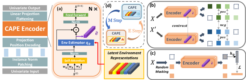
Figure 1: (a) CAPE encoder and environment estimator with latent representations; (b) Hierarchical environment contrasting for temporal and environment representations; (c) Random masking and reconstruction with environment estimation to capture universal patterns; (d) EM algorithm to iteratively optimize model parameters and environment representations.

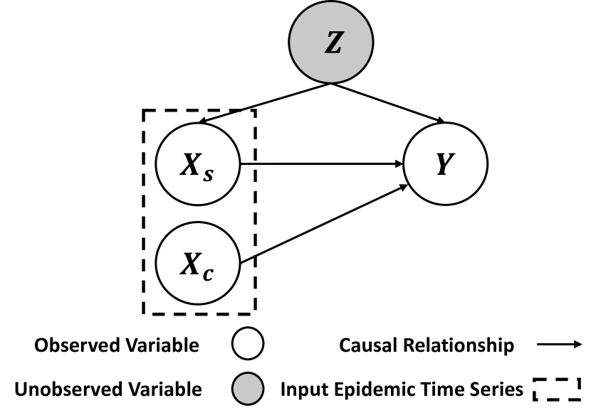
Figure 2: Structural causal model for epidemic foresting, where $Z$ refers to the environment states, and $X_{s}$ and $X_{c}$ refer to the spurious and causal factors of the input.

Our Solution. To integrate insights from extensive historical diseases and effectively model environmental factors, we propose Covariate-Adjusted Pretraining for Epidemic forecasting (CAPE) to capture the universal patterns of disease dynamics, as shown in Figure 2. Our approach addresses the challenges of optimizing the model with limited observations of a single disease infection trajectory and the complex influence of the environment by combining a pre-training framework with explicit environment modeling. Drawing on principles from causal analysis and covariate adjustment Runge et al. (2023), CAPE aims to estimate the latent environments and control for their influences for epidemic forecasting. Specifically, during the pre-training phase, CAPE utilizes environment-aware self-supervised learning, including random masking (Figure 2(c)) and hierarchical environment contrasting (Figure 2(b)), to enhance its understanding of the disease dynamics and environmental influence. Furthermore, an environment estimator is introduced, which estimates dynamic environments based on latent environment representations learned during pre-training using Expectation-Maximization algorithm. Our contributions can be summarized as follows:

1. We propose a novel epidemic pre-training framework, namely CAPE, that learns representations of environments and performs covariate adjustment on the input epidemic time series data, which aims to disentangle the inherited disease dynamics from the environment.

2. We assemble a diverse collection of epidemic time series datasets from various diseases and regions, serving as a crucial testbed for evaluating pre-trained epidemic forecasting models. This allows for extensive testing across multiple scenarios, including few-shot, zero-shot, cross-location, and cross-disease evaluations.

3. We demonstrate the effectiveness of pre-training on epidemic datasets, showcasing superior performance across various downstream datasets and settings. Notably, CAPE surpasses the best baseline by an average of 9.9% in the full-shot setting and 18.1% in the zero-shot setting across all tested downstream datasets.

4. We provide an in-depth analysis of how pre-training and environment estimation affect downstream performance and mitigate the impact of distribution shifts.

2 Related Work and Problem Definition

Epidemic Forecasting Models. Traditionally, epidemic forecasting employs models like ARIMA Sahai et al. (2020), SEIR He et al. (2020), and VAR Shang et al. (2021). ARIMA predicts infections by analyzing past data and errors, SEIR models population transitions using differential equations, and VAR captures linear inter-dependencies by modeling each variable based on past values. Recently, deep learning models—categorized into RNN-based, MLP-based, and transformer-based—have surpassed these methods. RNN-based models like LSTM Wang et al. (2020) and GRU Natarajan et al. (2023) use gating mechanisms to manage information flow. MLP-based models use linear layers Zeng et al. (2023) or multi-layer perceptrons Borghi et al. (2021); Madden et al. (2024) for efficient data-to-prediction mapping. Transformer-based models Wu et al. (2021); Zhou et al. (2021, 2022) apply self-attention to encode time series and generate predictions via a decoder. However, these models are limited in that they typically utilize data from only one type of disease without considering valuable insights and patterns from diverse disease datasets.

Pre-trained Time Series Models. To enhance performance and enable few-shot or zero-shot capabilities, transformer-based models often employ pre-training on large datasets, which typically use masked data reconstruction Zerveas et al. (2021); Rasul et al. (2023) or promote alignment across different contexts Fraikin et al. (2023); Zhang et al. (2022); Yue et al. (2022). For example, PatchTST Nie et al. (2022) segments time series into patches, masks some, and reconstructs the masked segments. Larger foundational models like MOMENT Goswami et al. (2024) aim to excel in multiple tasks (e.g., forecasting, imputation, classification) but require substantial data and computational resources. In the epidemic context, Kamarthi et al. Kamarthi & Prakash (2023) pre-trained on various diseases, improving downstream performance and highlighting pre-training’s potential in epidemic forecasting. Nevertheless, all these models overlook the influence of the environment, and zero-shot ability in epidemic forecasting, along with the factors affecting the pre-training process, remain unanswered. In this study, we introduce environment modeling and conduct a thorough analysis of these questions.

Problem Definition. In this study, we adopt a univariate setting: Given a historical time series input: $\mathbf{x}\in\mathbb{R}^{T\times 1}$, where $T$ is the size of lookback window, the goal of epidemic forecasting is to map $\mathbf{x}$ into target trajectories (e.g. infection rates): $\mathbf{y}\in\mathbb{R}^{h}$, where $h$ denotes the size of the forecast horizon. We define $X$ and $Y$ as the random variables of input $\mathbf{x}$ and target $\mathbf{y}$ respectively. During pre-training, a representation function $g_{\theta}:\mathbb{R}^{T\times 1}\to\mathbb{R}^{T\times d}$, where $d$ denotes the dimension of the latent space and $\theta$ being the parameter of the model, extracts universal properties from a large collection of epidemic time series datasets $\mathcal{D}_{\text{pre}}=\{D_{1}^{\prime},D_{2}^{\prime},\dots,D_{S}^{\prime}\}$. Then, a set of self-supervised tasks $\mathcal{T}_{\text{pre}}=\{\mathcal{T}_{i}\}_{i=1}^{R}$ is defined, where each task $\mathcal{T}_{i}$ transforms a sample $\mathbf{x}\sim\mathcal{D}_{\text{pre}}$ into a pair of new input and label: $(\mathbf{\tilde{x}},\mathbf{\tilde{y}})$, and optimizes a loss $\mathcal{L}_{\mathcal{T}_{i}}=\mathbb{E}_{\mathbf{x}\sim\mathcal{D}_{\text{pre}}}[\ell_{\mathcal{T}_{i}}(h_{\psi}(g_{\theta}(\mathbf{\tilde{x}})),\mathbf{\tilde{y}})]$, with $\ell_{\mathcal{T}_{i}}$ being the task-specific metric and $h_{\psi}$ the task-specific head.

3 Proposed Method

3.1 Model Design

3.1.1 Causal Analysis for Epidemic Forecasting

As environments influence both historical infection patterns and future disease spread, we draw inspiration from causal inference Zhou et al. (2023); Jiao et al. (2024) and introduce a Structural Causal Model where we treat the environment $Z$ as a confounder that influences both the independent variable (e.g., historical data $X$) and the dependent variable (e.g., future infections $Y$). Furthermore, we adopt a causal decomposition approach Mao et al. (2022) that separates $X$ into two components (Figure 2): (1) a spurious factor $X_{s}$ that is environment-dependent, and (2) a causal factor $X_{c}$ that remains environment-independent. Both factors influence the target $Y$, with $X_{s}$ reflecting the impact of environment $Z$. Since epidemic dynamics are driven by a finite set of critical factors, such as public health policies, we model $Z$ with the following assumption:

Assumption 3.1.

The environment variable $Z$ follows a categorical distribution $p(Z)$ and takes on one of $K$ discrete environmental states, denoted as $z_{k}$. Each state $z_{k}$ is associated with a unique latent representation $\mathbf{e}_{k}\in\mathbb{R}^{h_{e}}$, capturing the unique features specific to that environment.

In constructing a predictive model for input $\mathbf{x}$, we define $\hat{Y}$ as the predicted time series $\hat{\mathbf{y}}$ and model the predictive distribution $p_{\Theta}(\hat{Y}|X)$ using $f_{\Theta}(\mathbf{x})=h_{\psi}(g_{\theta}(\mathbf{x}))$, where $\Theta=\{\theta,\psi\}$. Training typically involves maximizing the log-likelihood of $p_{\Theta}(\hat{Y}|X)$, which in practice translates to minimizing the errors over the pre-training dataset $\mathcal{D}_{\text{pre}}$:

$$\Theta^{*}=\arg\min_{\Theta}-\frac{1}{|\mathcal{D}_{\text{pre}}|}\sum\nolimits_{(\mathbf{x},\mathbf{y})\in\mathcal{D}_{\text{pre}}}\|\mathbf{y}-f_{\Theta}(\mathbf{x}))\|^{2}.$$ (1)

As the environment $Z$ impacts the distribution of the observed data through $p(X,Y|Z)=p(X|Z)p(Y|X,Z)$, we formulate the following objective:

$$\small\begin{split}\Theta^{*}=&\arg\min\nolimits_{\Theta}\mathbb{E}_{p(Z)}[\mathbb{E}_{(\mathbf{x},\mathbf{y})\sim p(Y,X|Z)}[\|\mathbf{y}-f_{\Theta}(\mathbf{x}))\|^{2}]].\end{split}$$ (2)

The above equation suggests that the optimal $\Theta^{*}$ depends on the environment distribution $p(Z)$. If we simply maximize the likelihood $p_{\Theta}(\hat{Y}|X)$, the confounding effect of $Z$ on $X$ and $Y$ will mislead the model to capture the shortcut predictive relation between the input and the target trajectories, which necessitates explicit modeling of the environment during pre-training. Given that input infection trajectories inherently reflect the influence of the environment, it is crucial to develop mechanisms that disentangle the correlations between infection trajectories and environmental factors.

In this study, we switch to optimize $p_{\Theta}(\hat{Y}|do(X))$, where the do-operation intervenes the variable $X$ and removes the effects from other variables (i.e., $Z$ in our case), thus effectively isolating the disease dynamics from environmental influences. In practice, this operation is usually conducted via covariate adjustment, particularly backdoor adjustment Sun et al. , which controls for the confounder and uncovers the true causal effects of interest. The theoretical foundation for this is explained through: $p(Y|do(X))=\int p(Y|X,Z=z)p(Z=z)dz$ (see Appendix A.1). Under Assumption 3.1, this simplifies over different environmental states:

$$p(Y|do(X))=\sum\nolimits_{Z}p(Y|X,Z=z)p(Z=z).$$ (3)

However, obtaining detailed environmental information, or ${\bf e}_{k}$, can be challenging due to variability in data availability and quality. To address this, we resort to a data-driven approach that treats ${\bf e}_{k}$ as learnable parameters and thus allows us to dynamically infer the environmental distribution directly from the observed data. Specifically, we implement an environment estimator $q_{\phi}(Z|X)$ that infers the probability of environment states based on historical inputs together with the latent representations of each state. Then, we derive a variational lower bound (see Appendix A.1):

$$\log{p_{\Theta}(\hat{Y}|do(X))}\geq$$ (4)

$$\mathbb{E}_{q_{\phi}(Z|X)}\left[\log p_{\Theta}(\hat{Y}|X,Z)\right]-\operatorname{KL}\left(q_{\phi}(Z|X)\parallel p(Z)\right),$$

where the first term maximizes the model’s predictive power and the second term regularizes the environment estimator to output a distribution close to the prior distribution $p(Z)$.

3.1.2 Model Instantiation

To instantiate and train a model that performs the covariate adjustment, we need to model the environment estimator $q_{\phi}(Z|X)$ and the predictor $p_{\Theta}(\hat{Y}|X,Z)$.

Latent Environment Estimator $q_{\phi}(Z|X)$. We model $p(Z|X)$ using a latent environment estimator $q_{\phi}(Z|X)$. Since environmental influences vary over time, we apply patching Nie et al. (2022) to manage granularity in environment estimation. This prevents overly specific or generalized estimations that could obscure key temporal fluctuations. We divide the input $\mathbf{x}$ into $C$ non-overlapping patches, $\mathbf{x}=[\mathbf{x}_{1},\dots,\mathbf{x}_{C}]$, where $\mathbf{x}_{c}\in\mathbb{R}^{T/C}$. Then, a self-attention layer $f_{\text{enc}}$ captures temporal dependencies between patches, producing contextualized representations $\mathbf{h}^{(l)}_{c}=f_{\text{enc}}(\mathbf{x}^{(l)}_{c})$ for each patch at layer $l$. Subsequently, since the environment influences only the spurious component of the input, we introduce a transformation $\mathbf{W}_{s}^{(l)}$ to capture the spurious component of $\mathbf{h}^{(l)}_{c}$. Finally, we model $q_{\phi}(Z|X)$ as a cross-attention layer that captures the relation between each patch and the latent environment representations:

$$\pi_{k,c}^{(l)}=\operatorname{Softmax}\left((\mathbf{W}_{k}^{(l)}\mathbf{e}_{k})^{\top}\cdot(\mathbf{W}_{s}^{(l)}\mathbf{h}_{c}^{(l)})\right),$$ (5)

where $\pi_{k,c}^{(l)}$ is the output probability of the environment $z_{k}$ for the $c$-th patch, and $\mathbf{W}_{k}^{(l)}$ is a transformation layer for $\mathbf{e}_{k}$. Such operation not only takes into account the contextualized representation of the current time period, but also considers the latent environment representations, which made it possible to infer the densities of other environment distributions with different latent representations.

Epidemic Predictor $p_{\Theta}(\hat{Y}|X,Z)$. Unlike previous studies, which do not explicitly model environment states, we incorporate these states directly into the input using their latent representations $\mathbf{e}_{k}$. Specifically, we model the predictor $p_{\Theta}(\hat{Y}|X,Z)$ by employing a weighted sum over the combined representations of each environment and the input using Hadamard product, i.e., $f_{\text{enc}}(\mathbf{x}_{c}^{(l)})\odot\mathbf{e}_{k}$. Finally, we apply a feed-forward layer to compute the output representations, serving as the input for the next layer. Integrating these components, the CAPE encoder can be expressed as:

$$\small\mathbf{x}^{(l+1)}_{c}=\sigma\left(\mathbf{W}_{f}^{(l)}\sum_{k=1}^{K}\pi_{k,c}^{(l)}\left[f_{enc}({\mathbf{x}_{c}^{(l)}})\odot\mathbf{e}_{k}\right]\right),$$ (6)

where $\sigma$ represents the activation function and $\mathbf{W}_{f}^{(l)}$ denotes the learnable parameters of the feedforward layer. Assuming $L$ layers are stacked, we acquire the final representation $\mathbf{x}^{(L)}=[\mathbf{x}^{(L)}_{1},\mathbf{x}^{(L)}_{2},\ldots\mathbf{x}^{(L)}_{C}]=g_{\theta}({\bf x})\in\mathbb{R}^{C\cdot d}$ and apply a task-specific head to predict the target variable $\mathbf{y}=h_{\psi}(\mathbf{x}^{(L)})$, where $h_{\psi}$ is a linear transformation.

3.2 Pre-training Objectives for Epidemic Forecasting

CAPE captures diverse epidemic time series dynamics through self-supervised learning tasks that identify universal patterns in the pre-training dataset. While previous studies neglected the confounding effects of environmental factors on input-label pairs in $\mathcal{T}_{\text{pre}}$, CAPE seamlessly integrates environment estimation into the self-supervised framework.

Random Masking with Environment Estimation. To capture features from large unlabeled epidemic time series data, we employ a masked time series modeling task Kamarthi & Prakash (2023); Goswami et al. (2024) (Figure 2(c)) that masks 30% of input patches. As depicted in Figure 2, the generation of $X$ depends on the environment $Z$, indicating that accurate patch reconstruction requires capturing both temporal and environmental dependencies. Unlike prior studies that overlook the environment’s role, we utilize an environment estimator $q_{\phi}(Z|X)$ to infer $Z$, aiding both reconstruction and estimator training. During pre-training, input $\mathbf{x}$ is transformed into masked input and label pairs $(\tilde{\mathbf{x}},\mathbf{x})$, with the original time series serving as label $y$. The reconstruction $\hat{\mathbf{x}}=h_{\psi}(g_{\theta}(\tilde{\mathbf{x}}))$ is optimized using Mean Squared Error (MSE): $\mathcal{L}_{\text{recon}}(\mathbf{x},\hat{\mathbf{x}})=\text{MSE}(\hat{\mathbf{x}},\mathbf{x})$.

Hierarchical Environment Contrasting. Two consecutive time series samples, ${\bf x}$ and ${\bf x}^{\prime}$, can include overlapping regions when divided into multiple patches. These overlapping patches, although identical, can exhibit contextual variations influenced by their different adjacent patches. As indicated by Eq. (5), such variations can alter the latent patch-wise representations, leading to inconsistencies in the environmental estimates for the same patch across the samples. To ensure that each patch’s environment remains context-invariant, we propose a hierarchical environment contrasting scheme inspired by Yue et al. (2022). We define an aggregated latent environment representation $\hat{\mathbf{e}}^{(l)}_{c}=\sum_{k=1}^{K}\mathbf{e}_{k}\pi_{k,c}^{(l)}$ to represent the weighted environment states for the $c$-th patch. For contrastive loss computation, we use the combined representation $\hat{\mathbf{E}}_{j,c}^{(l)}=\sigma(\mathbf{W}_{f}^{(l)}(\hat{\mathbf{e}}^{(l)}_{c}\odot\mathbf{h}^{(l)}_{c}))$ for $c$-th patch of sample $j$. Additionally, $\hat{\mathbf{E}^{\prime}}_{j,c}^{(l)}$ denotes the representation in the context of $\mathbf{x}^{\prime}$. Finally, we compute a patch-wise contrastive loss:

$$\mathcal{L}_{\text{CL}}(j,c)=-\hat{\mathbf{E}}_{(j,c)}\cdot\hat{\mathbf{E}^{\prime}}_{(j,c)}$$

$$+\log\left(\sum_{b\in B}\exp\left(\hat{\mathbf{E}}_{(j,c)}\cdot\hat{\mathbf{E}^{\prime}}_{(b,c)}\right)+\mathbb{I}_{j\neq b}\exp\left(\hat{\mathbf{E}}_{(j,c)}\cdot\hat{\mathbf{E}}_{(b,c)}\right)\right)$$

$$+\log\left(\sum_{t\in\Omega}\exp\left(\hat{\mathbf{E}}_{(j,c)}\cdot\hat{\mathbf{E}^{\prime}}_{(j,t)}\right)+\mathbb{I}_{c\neq t}\exp\left(\hat{\mathbf{E}}_{(j,c)}\cdot\hat{\mathbf{E}}_{(j,t)}\right)\right).$$

where $B$ is the batch size, $\Omega$ denotes the overlapping patches, and $\mathbb{I}$ is the indicator function. The above equation contains three key terms: (1) The first term encourages the representations of the same patch from two different contexts to be similar, which preserves the context-invariant nature of environments. (2) The second term (Instance-wise Contrasting) treats $\hat{\mathbf{e}}^{(l)}_{c}$ from different samples in the batch as negative pairs, which promotes dissimilar representations, and enhances diversity among instances. (3) The third term (Temporal Contrasting) treats the representations of different patches from overlapping regions ($\Omega$) as negative pairs, which encourages differences across temporal contexts.

Pre-Training Loss. Given a batch of $B$ samples $\mathbf{X}\in\mathbb{R}^{B\times T}$, we combine the reconstruction loss and the contrastive loss, yielding the final loss function for pre-training:

$$\mathcal{L}_{\text{final}}=\sum\nolimits_{\mathbf{x}\in\mathbf{X}}\mathcal{L}_{\text{recon}}(\mathbf{x},\hat{\mathbf{x}})+\alpha\,\mathcal{L}_{\text{CL}}(\hat{\mathbf{E}}^{(L)},\hat{\mathbf{E}}^{\prime(L)}),\;\mathbf{X}\sim\mathcal{D}_{\text{pre}}$$

where $L$ is the number of layers, and $\alpha$ is the hyperparameter used to balance the contrastive loss and the reconstruction loss. Further analysis can be found in Appendix A.10.

3.3 Optimization of the CAPE Framework

To effectively maximize the variational lower bound in Eq. (4), we employ the Expectation-Maximization (EM) algorithm to iteratively update the latent environments and epidemic predictor. The pseudo algorithm for the optimization procedure is provided in Appendix A.3.

E-Step: Estimating Latent Environments. In the E-step, we aim to identify the environment states $Z$ and the corresponding distribution $p(Z)$ that result in the target distribution $p(Y)$. This involves maximizing the expected likelihood of $p(Y|Z)$ given $p(Z)$. We freeze the epidemic predictor $p_{\Theta}(\hat{Y}|X,Z)$ and the environment estimator $q_{\phi}(Z|X)$, treating them as oracles, which means $p_{\Theta}(\hat{Y}|X,Z)=p(Y|X,Z)$ and $q_{\phi}(Z|X)=q(Z|X)$. While actively updating the environment representations $\mathbf{E}=[\mathbf{e}_{1},\mathbf{e}_{2},...\mathbf{e}_{k}]$, the optimization of the environment states $Z$ is learned through maximizing $\mathbb{E}_{p(Z)}[p(Y|Z)]=\mathbb{E}_{p(X)}[\mathbb{E}_{q_{\phi}(Z|X)}p_{\Theta}(Y|X,Z)]$, which is equivalent to minimizing the expected reconstruction loss:

$$\mathbf{E}^{t+1}\leftarrow\arg\min\nolimits_{\mathbf{E}}\left[\mathbb{E}_{\mathbf{x}\sim p(X)}[\mathcal{L}_{\text{recon}}(\mathbf{x},\hat{\mathbf{x}})]\right].$$ (7)

We use subscript $t$ to denote the pre-update distribution and derive the updated distribution $p^{t+1}(Z)$ as $q^{t+1}_{\phi_{t}}(Z)$, along with the updated environment representations $\mathbf{E}^{t+1}$.

M-Step: Optimizing Epidemic Predictor. In the M-step, we aim to optimize the epidemic predictor by maximizing its predictive power and regularizing the environment distribution. During this step, the environment representations $\mathbf{E}^{t+1}$ are held fixed. We have the following theorem:

Theorem 3.2.

Assuming $q^{t+1}_{\phi_{t}}(Z)=p^{t+1}(Z)$ and an L2 norm is applied on $\phi$, the variational lower bound in Eq. (4) can be approximated as follows:

$$\mathbb{E}_{p(X)}\left[\mathbb{E}_{q^{t+1}_{\phi_{t}}(Z|X)}\left[\log p^{t+1}_{\Theta_{t+1}}(\hat{Y}|X,Z)\right]\right]-C,$$ (8)

which is equivalent to minimizing the expected reconstruction loss $\mathbb{E}_{\mathbf{x}\sim p(X)}[\mathcal{L}_{recon}(\mathbf{x},\hat{\mathbf{x}})]$ .

The detailed proof can be found in Appendix A.1. Theorem 3.2 indicates that the optimization of the model’s predictive ability can be approximated by Eq. (8), which corresponds to the expectation of $\mathcal{L}_{recon}$. To further enhance robustness, the contrastive loss is combined to regularize the environment estimator. Therefore, the overall optimization objective becomes minimizing the final pre-training loss:

$$\Theta_{t+1}\leftarrow\arg\min\nolimits_{\Theta}\left[\mathcal{L}_{\text{final}}(\mathbf{X},\hat{\mathbf{X}},\mathbf{E}^{t+1})\right].$$ (9)

Table 1: Univariate forecasting results with horizons ranging from 1 to 16 future steps. The lookback window length is set to 36 and all models are evaluated using MSE. Note that performance rankings are distinguished by color coding: Best, Second Best, Third Best. $\Delta(\%)$ stands for the relative improvement of CAPE over the baselines in terms of average MSE over all horizons.

Dataset	Horizon	Statistical Model	RNN-Based		MLP-Based	Transformer-Based						CAPE
		ARIMA	LSTM	GRU	Dlinear	Non-Pre-trained			Pre-trained
						Informer	Autoformer	Fedformer	PEM	MOMENT	PatchTST
ILI USA	1	0.138	0.338	0.259	0.220	0.175	0.457	0.368	0.179	0.269	0.195	0.155
	2	0.203	0.377	0.301	0.247	0.370	0.710	0.380	0.226	0.321	0.264	0.200
	4	0.354	0.458	0.386	0.376	0.517	0.670	0.433	0.304	0.397	0.385	0.270
	8	0.701	0.579	0.529	0.506	0.597	0.842	0.570	0.538	0.510	0.535	0.404
	16	1.121	0.691	0.626	0.617	0.812	0.835	0.701	0.570	0.610	0.485	0.516
	Avg	0.503	0.489	0.420	0.393	0.494	0.703	0.490	0.363	0.421	0.373	0.309
	$\Delta$ (%)	38.57%	36.81%	26.43%	21.37%	37.45%	56.05%	36.94%	14.88%	26.60%	17.16%	-
ILI Japan	1	0.358	1.426	1.213	1.016	0.405	0.515	0.525	0.470	0.325	0.413	0.290
	2	0.772	1.635	1.458	1.294	0.666	0.855	1.151	0.755	0.586	0.698	0.535
	4	1.720	1.975	1.870	1.758	1.234	1.150	1.455	1.207	1.082	1.147	0.944
	8	2.981	2.373	2.365	2.285	1.688	1.866	2.012	1.810	1.706	1.708	1.650
	16	2.572	2.023	2.010	2.007	1.551	2.654	4.027	1.766	2.054	1.688	1.911
	Avg	1.680	1.886	1.783	1.672	1.109	1.408	1.834	1.202	1.151	1.131	1.066
	$\Delta$ (%)	36.55%	43.48%	40.21%	36.24%	3.88%	24.29%	41.88%	11.31%	7.38%	5.74%	-
Measles	1	0.071	0.182	0.143	0.133	0.066	0.203	0.321	0.085	0.113	0.094	0.083
	2	0.120	0.223	0.176	0.184	0.153	0.257	0.817	0.128	0.138	0.127	0.112
	4	0.225	0.310	0.258	0.296	0.288	0.331	0.226	0.213	0.186	0.205	0.161
	8	0.483	0.567	0.471	0.512	0.501	0.671	0.403	0.417	0.351	0.377	0.310
	16	1.052	1.110	1.013	1.088	0.904	1.115	0.754	0.806	0.818	0.722	0.752
	Avg	0.390	0.478	0.412	0.443	0.382	0.515	0.504	0.330	0.321	0.305	0.269
	$\Delta$ (%)	31.03%	43.72%	34.71%	39.28%	29.58%	47.77%	46.63%	18.49%	16.20%	11.80%	-
Dengue	1	0.244	0.250	0.261	0.224	0.255	0.525	0.521	0.225	0.420	0.240	0.223
	2	0.373	0.343	0.343	0.316	0.450	0.807	0.670	0.314	0.579	0.334	0.302
	4	0.696	0.564	0.579	0.560	0.798	0.957	0.766	0.571	0.661	0.586	0.561
	8	1.732	1.168	1.183	1.256	1.239	1.684	1.539	1.223	1.308	1.292	1.046
	16	4.082	3.876	3.315	3.109	2.659	3.364	2.934	3.376	2.532	2.537	2.509
	Avg	1.426	1.240	1.136	1.093	1.080	1.467	1.286	1.142	1.100	1.000	0.892
	$\Delta$ (%)	37.45%	28.06%	21.48%	18.39%	17.41%	39.20%	30.64%	21.89%	18.91%	10.80%	-
Covid	1	33.780	22.592	22.009	23.811	34.161	42.049	28.130	25.088	32.376	23.645	21.548
	2	33.193	23.460	22.542	24.809	24.883	30.631	28.059	23.123	35.418	25.047	22.224
	4	32.482	24.729	24.816	26.345	31.328	41.029	29.432	23.889	36.251	24.224	22.476
	8	36.573	31.019	33.934	33.081	35.964	55.812	41.791	31.217	40.429	31.548	28.403
	16	42.910	43.820	41.432	47.561	50.244	47.993	69.976	51.265	52.590	43.309	40.555
	Avg	35.787	29.124	28.947	31.121	35.316	43.503	39.478	30.917	39.413	29.555	26.559
	$\Delta$ (%)	25.79%	8.81%	8.25%	14.66%	24.80%	38.95%	32.72%	14.10%	32.61%	10.14%	-

Table 2: Few-shot learning results with horizons ranging from 1 to 16 future steps. The length of the lookback window is set to 36. Each model is evaluated after being trained on 20%, 40%, 60%, and 80% of the full training data. $\Delta(\%)$ stands for the relative improvement of the model after training with 20% more data in terms of average MSE over all horizons. The full result is shown in Appendix A.5.

Dataset/Model	CAPE					PatchTST					Dlinear					MOMENT					PEM
	20%	40%	60%	80%	100%	20%	40%	60%	80%	100%	20%	40%	60%	80%	100%	20%	40%	60%	80%	100%	20%	40%	60%	80%	100%
ILI USA	2.121	1.400	0.760	0.369	0.309	2.114	1.219	0.677	0.401	0.373	2.822	1.594	0.816	0.412	0.346	3.990	1.847	0.913	0.459	0.381	2.143	1.261	0.681	0.419	0.353
$\Delta$(%)	-	33.99%	45.71%	51.45%	16.26%	-	42.34%	44.45%	40.77%	6.98%	-	43.53%	48.78%	49.51%	16.02%	-	53.69%	50.58%	49.72%	17.00%	-	41.13%	46.00%	38.33%	15.76%
Dengue	13.335	6.386	2.356	1.511	0.892	13.712	7.304	2.771	1.678	0.984	15.828	8.420	2.850	1.748	1.080	15.697	7.536	2.816	1.733	1.358	12.90	7.055	2.745	1.707	0.964
$\Delta$(%)	-	52.07%	63.12%	35.87%	40.95%	-	46.72%	62.06%	39.43%	41.39%	-	46.81%	66.15%	38.64%	38.19%	-	52.00%	62.63%	38.45%	21.65%	-	45.32%	61.09%	37.79%	43.51%
Measles	0.483	0.600	0.381	0.285	0.269	0.863	0.834	0.448	0.359	0.306	1.194	1.130	0.602	0.478	0.394	1.661	0.915	0.425	0.471	0.500	0.670	0.896	0.430	0.364	0.306
$\Delta$(%)	-	-24.22%	36.50%	25.20%	5.61%	-	3.36%	46.25%	19.91%	14.81%	-	5.36%	46.64%	20.63%	17.58%	-	44.91%	53.55%	-10.59%	-6.16%	-	-33.87%	51.91%	15.35%	15.93%

4 Experiment

4.1 Experiment Setup

Datasets. For pre-training CAPE, PatchTST, and PEM, we manually collected 17 distinct weekly-sampled diseases from Project Tycho van Panhuis et al. (2018). For evaluation, we utilize five downstream datasets covering various diseases and locations: ILI USA Centers for Disease Control and Prevention (2023a), ILI Japan National Institute of Infectious Diseases (2023), COVID-19 USA Dong et al. (2020), Measles England Lau et al. (2020a), and Dengue across countries OpenDengue (2023). Additionally, RSV Centers for Disease Control and Prevention (2023c) and Monkey Pox Centers for Disease Control and Prevention (2023b) infections in the US are used to test zero-shot performance. More details can be found in Appendix A.2.

Baselines. For baselines, we leverage the models from the comprehensive toolkit EpiLearn Liu et al. (2024a). To provide a comprehensive evaluation, we compare CAPE with two sets of models: non-pretrained and pre-trained. Non-pretrained models include statistical methods like ARIMA Panagopoulos et al. (2021), RNN-based Wang et al. (2020); Natarajan et al. (2023) approaches such as LSTM and GRU, the linear model DLinear Zeng et al. (2023), and transformer-based methods Wu et al. (2021); Zhou et al. (2021, 2022). For pre-trained models, we evaluate popular approaches including PatchTST Nie et al. (2022), PEM Kamarthi & Prakash (2023), and a time series foundation model MOMENT Goswami et al. (2024). More experimental details can be found in Appendix A.3.

4.2 Baseline Comparison

We now evaluate the CAPE model under three settings: fine-tuning, few-shot fine-tuning, and zero-shot forecasting.

4.2.1 Fine-Tuning (Full-Shot Setting)

For non-pre-trained models, we train the entire model on the training split, while for pre-trained models, we fine-tune on downstream datasets by transferring the task-specific head $h_{\psi}$ from pre-training to the forecasting task. We evaluate short-term and long-term performance by reporting MSE across horizons from 1 to 16. From Table 1, we observe: (a) CAPE achieves the best average MSE across all downstream datasets. It outperforms the best baseline by 9.91% on average and up to 14.85%. On the COVID dataset, CAPE performs best across all horizons, showing effectiveness on novel diseases. (b) Models like PEM, PatchTST, and MOMENT consistently rank second or third on 4 out of 5 downstream datasets. The best pre-trained model (excluding CAPE) outperforms the best non-pre-trained model by 6.223% on average. Among them, PatchTST has the highest average performance, surpassing PEM by 5.51% and MOMENT by 10.45%. Additionally, PEM outperforms MOMENT by 4.86%, indicating the importance of epidemic-specific pre-training. (c) Informer consistently outperforms Autoformer and Fedformer by 24.40% and 17.90% respectively, due to its sparse attention mechanism that reduces overfitting. Informer also surpasses Dlinear by 1.90%, suggesting that careful selection of model size and parameters is crucial for optimal performance. (d) Furthermore, environment modeling proves valuable, as CAPE consistently outperforms PatchTST, which shares a similar design. While both models are pre-trained on the epidemic-specific datasets, CAPE surpasses PatchTST by 11.13%.

4.2.2 Few-Shot and Zero-Shot Performance

Few-Shot Forecasting. In real-world scenarios, predicting outbreaks of diseases unknown or in new locations is challenging for purely data-driven models due to limited initial data. Thus, few-shot or zero-shot forecasting capabilities are essential for epidemic models. To simulate a few-shot scenario, we reduce the original training data from 100% to [20%, 40%, 60%, 80%]. We report the average MSE across 1 to 16 time steps. From Table 8, we make the following observations: (a) With an increasing volume of training materials, the performance of all models consistently improves. (b) CAPE achieves the best performance in most scenarios, demonstrating the superior few-shot ability. (c) Compared with models pre-trained on epidemic-specific datasets, Dlinear failed to achieve better performance when only 20% of training data is available. However, Dlinear is able to outperform MOMENT on ILI USA and Measles datasets when both models are trained or fine-tuned using 20% training data, which indicates the importance of pre-training. (d) Though CAPE achieves the best average performance on the ILI USA dataset when the training material is reduced, it achieves a good performance in short-term forecasting from 1 to 4 weeks (see Appendix A.5).

Table 3: Zero-shot performance with a lookback window length of 12. All results are averaged over 4 weeks or days in the future. $\Delta(\%)$ stands for the relative improvement of CAPE over the baselines.

Dataset	$\Delta$ (%)	CAPE	PatchTST	PEM	MOMENT
ILI USA	9.26%	0.147	0.164	0.162	0.549
ILI Japan	17.06%	0.705	0.907	0.850	2.062
Measles	3.97%	0.145	0.167	0.159	0.533
Monkey Pox	20.00%	0.0004	0.0005	0.0005	0.0013
Dengue (mixed)	10.17%	0.371	0.427	0.413	1.624
RSV	26.06%	0.834	1.128	1.260	1.849
Covid (daily interval)	13.80%	5.173	6.001	6.320	18.881

Zero-Shot Forecasting. To further demonstrate the potential of our model, we evaluate CAPE in a zero-shot setting. Specifically, for transformer-based models, we retain the pre-training head and freeze all parameters during testing. All models are provided with a short input sequence of 12 time steps and tasked with predicting infections for the next 4 time steps. From Table 3, we make the following observations: (a) CAPE outperforms baselines across all downstream datasets, showing superior zero-shot forecasting ability. (b) Models pre-trained on epidemic-specific datasets achieve better performance compared to those pre-trained without epidemic-specific data (MOMENT). This indicates the necessity of choosing domain-specific materials for pre-training.

4.3 Ablation Study

We conducted an ablation study to assess CAPE’s components (Table 4). Replacing environment estimators with non-disentangling self-attention layers consistently worsened performance across all datasets, notably increasing ILI USA’s MSE from 0.309 to 0.532, underscoring the importance of environmental factors. Similarly, removing contrastive loss while retaining environment estimators raised Measles’ MSE from 0.269 to 0.344, with smaller increases for ILI USA and Dengue. Training CAPE directly on downstream datasets without pre-training also decreased performance, with MSE rising to 0.319 (ILI USA), 0.326 (Measles), and 1.162 (Dengue), though less than removing environment estimation. These results indicate that all CAPE components are essential for optimal forecasting and that tailoring component emphasis to dataset characteristics can further enhance performance.

Table 4: Ablation study of removing components from CAPE.

Dataset	Model	H=1	H=2	H=4	H=8	H=16	Avg
ILI USA	CAPE	0.155	0.200	0.270	0.404	0.516	0.309
	w/o Env	0.326	0.448	0.508	0.642	0.735	0.532
	w/o Contrast	0.174	0.241	0.335	0.492	0.570	0.363
	w/o Pretrain	0.158	0.202	0.283	0.408	0.545	0.319
Measles	CAPE	0.069	0.096	0.155	0.280	0.743	0.269
	w/o Env	0.083	0.111	0.168	0.407	0.755	0.304
	w/o Contrast	0.090	0.124	0.276	0.431	0.801	0.344
	w/o Pretrain	0.074	0.113	0.223	0.402	0.816	0.326
Dengue	CAPE	0.218	0.301	0.540	1.193	2.210	0.892
	w/o Env	0.232	0.316	0.484	1.089	3.622	1.149
	w/o Contrast	0.198	0.273	0.460	1.128	3.329	1.078
	w/o Pretrain	0.210	0.276	0.449	1.115	3.759	1.162

4.4 Transferability

Cross-Location. We include measles data from the USA in the pre-training dataset. To evaluate our model’s ability to adapt to cross-region data, we incorporate measles outbreak data from the UK into the downstream datasets. As shown in Table 4, the pre-trained CAPE outperforms the non-pre-trained version by 17.48%. While we pre-train our model with influenza data from the USA, the zero-shot evaluation on the influenza outbreak in Japan also shows superior performance, underscoring the crucial role of pre-training in enabling generalization to novel regions.

Cross-Disease. While we include various types of diseases in our pre-training dataset, novel diseases including Dengue (non-respiratory) and COVID-19 that are unseen in the pre-training stage are incorporated during the downstream evaluation. The ability of our model to adapt to novel diseases is proven compared to the version not pre-trained on the Dengue dataset (Table 4), improving which by 23.24%, as well as the superior zero-shot performance on the COVID dataset (Table 3), which surpasses the MOMENT that is not pre-trained on other diseases by 72.60%.

Cross-Interval. While we only pre-train using weekly-sampled data, our model outperformed the non-pre-trained version on the irregularly sampled Dengue dataset, demonstrating robustness to different time intervals. Additionally, on the daily-sampled COVID-19 dataset, our model maintained strong zero-shot performance, further illustrating its ability to generalize across varying temporal resolutions.

4.5 Deeper Analysis

Impact of Pre-Training Epochs. Evaluating four downstream datasets (Figure 3), we find that increasing pre-training epochs consistently improves performance on Measles and COVID datasets but degrades it for ILI USA. Additionally, models with more environment states $K$ perform better as pre-training epochs increase.

Figure 3: Downstream performance with different numbers of environments and pre-training epochs.

Impact of Pre-Training Materials. We examine potential biases in our pre-training dataset by splitting it into respiratory and non-respiratory diseases. As shown in Figure 4, with similar volumes of pre-training data, the model performs better on downstream datasets when their disease types align with the pre-training data (e.g., respiratory diseases). However, the size of the pre-training material has a more significant impact on downstream performance.

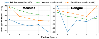
Figure 4: Downstream performance variation when the model is pre-trained with either respiratory or non-respiratory diseases only.

Impact of Pre-Training Material Scale. To explore how the pre-training material scale affects downstream performance, we scaled the original pre-training dataset and test on downstream datasets. As shown in Figure 5, a sudden performance boost is observed at around a 60% reduction for both Measles and Dengue datasets.

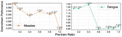
Figure 5: Downstream performance across pre-training ratios.

Tackling Distribution Shift. In this study, distribution shifts refer to changes in infection patterns observed from the training set to the test set. To evaluate distribution shifts, we compute the Central Moment Discrepancy (CMD) score Zellinger et al. (2017) between training and test distributions for each disease (see Appendix A.8). Figure 6 shows that our model with environment estimation achieves the lowest CMD score, demonstrating its effectiveness in mitigating the impact of temporal distribution shifts.

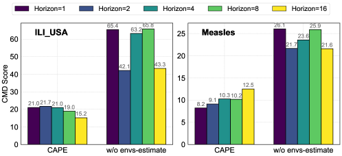
Figure 6: We report the CMD scores of the embeddings produced by CAPE with and without environment estimation, which quantify distributional differences between the training and test sets.

Disentangling Disease Dynamics. We validate our model’s ability to capture intrinsic disease dynamics by extracting latent embeddings from various datasets and computing the Davies-Bouldin Index (DBI) for each pair. As shown in Figure 7, CAPE consistently achieves lower DBI scores than PatchTST across all pairs, demonstrating its superior effectiveness in distinguishing diseases and separating disease-specific patterns from environmental influences.

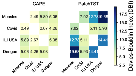
Figure 7: Davies-Bouldin Index score between the embeddings of each pair of downstream datasets, output by the pre-trained model without fine-tuning. A visualization is shown in Appendix A.9.

5 Conclusion

We present Covariate-Adjusted Pre-Training for Epidemic time series forecasting, showcasing the benefits of pre-training and environment modeling. While leveraging pre-training materials, CAPE explicitly learns latent representations of the environment and performs backdoor adjustment. Extensive experiments validate CAPE’s effectiveness in various settings, including few-shot and zero-shot.

Appendix A Appendix

A.1 Theoretical Analysis

A.1.1 Derivation for do-operation

We derive a tractable form for $\log p_{\Theta}(\hat{Y}|do(X))$, leveraging two rules of do-calculus.

Do-Calculus Rules.

Consider a causal DAG $\mathcal{A}$ with nodes $B$, $D$, and $Z$. Let $\mathcal{A}_{B}$ denote the intervened graph by removing all arrows entering $B$, and $\mathcal{A}^{B}$ the graph by removing all arrows leaving $B$. The rules are:

1. Action/Observation Exchange:

$$P(D|do(B),do(Z))=P(D|do(B),Z),$$

if $(D\perp\!\!\!\perp Z|B)$ in $\mathcal{A}^{Z}_{B}$.

2. Insertion/Deletion of Actions:

$$P(D|do(B),do(Z))=P(D|do(B)),$$

if $(D\perp\!\!\!\perp Z|B)$ in $\mathcal{A}^{BZ}$.

We consider a causal graph with variables $Z$, $X$, and $\hat{Y}$, as shown in Figure 2. Starting with the law of total probability:

$$\small P(\hat{Y}|do(X))=\int_{z}P(\hat{Y}|do(X),Z=z)P(Z=z|do(X))dz.$$ (10)

Step 1: Action/Observation Exchange. Using $(\hat{Y}\perp\!\!\!\perp X|Z)$ in $\mathcal{A}^{X}$, we apply the exchange rule:

$$P(\hat{Y}|do(X),Z=z)=P(\hat{Y}|X,Z=z).$$ (11)

Step 2: Insertion/Deletion of Actions. Using $(Z\perp\!\!\!\perp X)$ in $\mathcal{A}^{X}$, we simplify:

$$P(Z=z|do(X))=P(Z=z).$$ (12)

Substituting these into (10), we obtain:

$$P(\hat{Y}|do(X))=\int_{z}P(\hat{Y}|X,Z=z)P(Z=z)dz.$$ (13)

The result can be compactly written as:

$$p_{\Theta}(\hat{Y}|do(X))=\mathbb{E}_{p_{0}(Z)}\left[p_{\theta}(\hat{Y}|X,Z)\right],$$ (14)

where $p_{0}(Z)$ denotes the prior distribution of environments. Do-calculus rules simplify interventional distributions by leveraging independence properties, enabling tractable objectives for causal inference.

A.1.2 Derivation for Variational Lower Bound

Below we show the derivation for the variational lower bound in Eq. (4).

$$\quad\log\sum_{z}p_{\Theta}(\hat{Y}|X,Z=z)P(Z=z)$$ (15)

$$=\log\sum_{z}p_{\Theta}(\hat{Y}|X,Z=z)p(Z=z)\frac{q_{\phi}(Z=z|X)}{q_{\phi}(Z=z|X)}$$

$$\geq\sum_{z}q^{t+1}_{\phi}(Z=z|X)\log p_{\Theta}(\hat{Y}|X,Z=z)\frac{p(Z=z)}{q_{\phi}(Z=z|X)}\quad$$

(Jensen’s Inequality)

$$=\sum_{z}q_{\phi}(Z=z|X)\log p_{\Theta}(\hat{Y}|X,Z=z)$$

$$\quad\quad\quad\quad\quad\quad\quad-\sum_{z}q_{\phi}(Z=z|X)\log\frac{q_{\phi}(Z=z|X)}{p(Z=z)}$$

$$=\mathbb{E}_{q_{\phi}(Z|X)}\left[\log p_{\Theta}(\hat{Y}|X,Z)\right]-KL\left(q_{\phi}(Z|X)\parallel p(Z)\right)$$

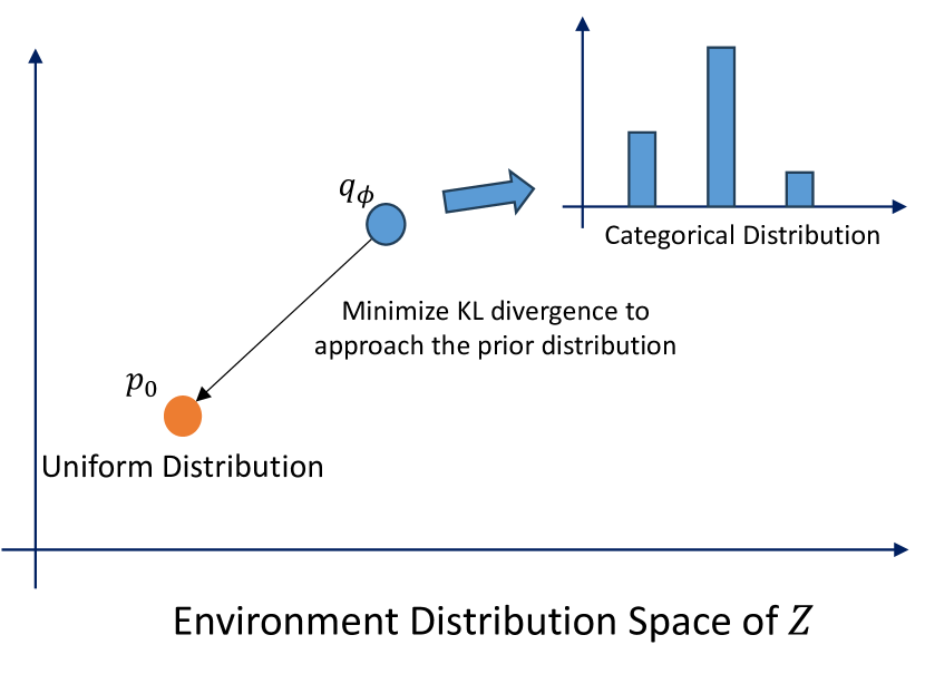
(a) Previous Method

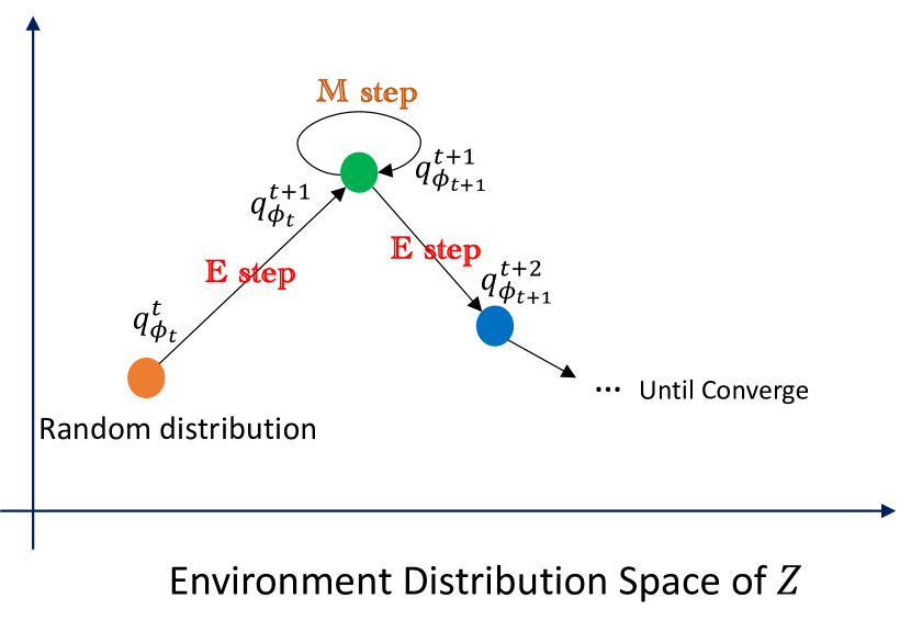
(b) Ours

Figure 8: Comparison between previous approach and our implementation.

A.1.3 Proof of Theorem 3.2

In this section, we provide the theoretical analysis of our optimization method, and an over is shown in Figure 8. Before proving Theorem 3.2, we prove the following theorem:

Theorem A.1.

Given the environment estimator before update $q_{\phi_{t}}$ and after update $q_{\phi_{t+1}}$, assuming the training process converges, then minimizing the KL divergence from $q_{\phi_{t+1}}$ to $q_{\phi_{t}}$, i.e., $\text{KL}(q_{\phi_{t+1}}||q_{\phi_{t}})$, is equivalent to applying an L2 norm on the parameters of the environment estimator $q_{\phi}$.

Proof.

Since $q_{\phi}$ only involves linear transformations and a softmax function, we argue that minimizing the KL loss between $q_{\phi}^{t}$ and $q_{\phi}^{t+1}$ is equivalent to minimizing the difference between $\phi^{t}$ and $\phi^{t+1}$.

Firstly, the logits $s_{i}$ are computed as: $s_{i}=\mathbf{W}_{k}^{(l)}\mathbf{e}^{k}$. A change in $\mathbf{W}_{k}^{(l)}$ , denoted as $\Delta\mathbf{W}_{k}^{(l)}$ , modifies $s_{i}$ as $\Delta s_{i}=(\Delta\mathbf{W}_{k}^{(l)})\mathbf{e}^{k}$. The change in $s_{i}$ is linear with respect to $\Delta\mathbf{W}_{k}^{(l)}$ and $\mathbf{e}^{k}$ . Therefore, a small change in $\mathbf{W}_{k}^{(l)}$ leads to proportionally small changes in $s_{i}$.

Secondly, the Softmax function introduces nonlinear coupling between logits $s_{i}$ , as the output probabilities $\pi_{i}$ depend not only on $s_{i}$ but also on all other logits $s_{j}$ . For a small change in $s_{i}$ , the change in $\pi_{i}$ can be approximated using the gradient of the Softmax $\frac{\partial\pi_{i}}{\partial s_{i}}=\pi_{i}(1-\pi_{i})$, $\frac{\partial\pi_{i}}{\partial s_{j}}=-\pi_{i}\pi_{j}\quad\text{for }i\neq j$. Thus, a change in $\mathbf{W}k^{(l)}$ affects $\pi_{i}$ as $\Delta\pi_{i}\approx\pi_{i}(1-\pi_{i})\Delta s_{i}-\sum_{j\neq i}\pi_{i}\pi_{j}\Delta s_{j}$. This implies that the change of the output $\Delta\pi_{i}$ shrinks proportionally with the change of parameters $\Delta\mathbf{W}_{k}$.

Lastly, for small parameter changes, we can approximate the KL divergence between the two categorical distributions using a second-order Taylor expansion around $q_{\phi}^{t}$. The KL divergence is defined as:

$$\text{KL}\left(q_{\phi}^{t}\parallel q_{\phi}^{t+1}\right)=\sum_{i}\pi_{i}^{t}\log\left(\frac{\pi_{i}^{t}}{\pi_{i}^{t+1}}\right).$$ (16)

Expanding $\log\left(\frac{\pi_{i}^{t}}{\pi_{i}^{t+1}}\right)$ around $\pi_{i}^{t}$ using the Taylor series for $\log(1+x)$ where $x=-\frac{\Delta\pi_{i}}{\pi_{i}^{t}}$ and keeping terms up to second order, we obtain:

$$\log\left(\frac{\pi_{i}^{t}}{\pi_{i}^{t+1}}\right) =\log\left(1+\frac{\pi_{i}^{t}-\pi_{i}^{t+1}}{\pi_{i}^{t}}\right)$$ (17)

$$=\log\left(1-\frac{\Delta\pi_{i}}{\pi_{i}^{t}}\right)\approx-\frac{\Delta\pi_{i}}{\pi_{i}^{t}}-\frac{1}{2}\left(\frac{\Delta\pi_{i}}{\pi_{i}^{t}}\right)^{2}.$$

Substituting this into the KL divergence expression and ignoring higher-order terms (since $\Delta\pi_{i}$ is small), we get:

$$\text{KL}\left(q_{\phi}^{t}\parallel q_{\phi}^{t+1}\right) \approx\sum_{i}\pi_{i}^{t}\left(-\frac{\Delta\pi_{i}}{\pi_{i}^{t}}-\frac{1}{2}\left(\frac{\Delta\pi_{i}}{\pi_{i}^{t}}\right)^{2}\right)$$ (18)

$$=-\sum_{i}\Delta\pi_{i}-\frac{1}{2}\sum_{i}\frac{(\Delta\pi_{i})^{2}}{\pi_{i}^{t}}.$$

Since $\sum_{i}\Delta\pi_{i}=0$ (as probabilities sum to one), the first term vanishes, leaving:

$$\text{KL}\left(q_{\phi}^{t}\parallel q_{\phi}^{t+1}\right)\approx\frac{1}{2}\sum_{i}\frac{(\Delta\pi_{i})^{2}}{\pi_{i}^{t}}.$$ (19)

Substituting the expression for $\Delta\pi_{i}$ from above and noting that $\Delta s_{i}$ is linear in $\Delta\phi$, we observe that the KL divergence is a quadratic function of $\Delta\phi$. Therefore, for small $\Delta\phi$, the KL divergence can be approximated as:

$$\mathcal{L}_{\text{KL}}\approx\frac{1}{2}\sum_{i}\frac{(\Delta\pi_{i})^{2}}{\pi_{i}^{t}}\propto\|\Delta\phi\|^{2}=\|\phi^{t}-\phi^{t+1}\|^{2}.$$ (20)

Thus, minimizing the KL divergence is approximately equivalent to minimizing $\|\phi^{t}-\phi^{t+1}\|^{2}$. In our setting, we use weight decay to regularize the model, which indirectly helps control the KL loss. Weight decay adds an L2 penalty to the loss function that encourages smaller parameter values, effectively shrinking the magnitude of the weights during training. The update rule for parameters with weight decay is given by: $\phi_{t+1}=\phi_{t}-\alpha\cdot\nabla_{\phi}\mathcal{L}_{\text{original}}-\alpha\cdot\lambda\phi_{t}$, where $\alpha$ is the learning rate and $\lambda$ is the weight decay coefficient. The total KL loss can be approximated as:

$$\mathcal{L}_{\text{kl}}\approx\|\phi^{t}-\phi^{t+1}\|^{2}=\alpha^{2}\|\nabla_{\phi}\mathcal{L}_{\text{original}}+\lambda\phi_{t}\|^{2}.$$ (21)

When the training process converges to a minimum, the task-related gradients ($\nabla_{\phi}\mathcal{L}_{\text{original}}$) become small and nearly zero, and the KL loss becomes dominated by the weight decay term, and the approximation simplifies to: $\mathcal{L}_{\text{kl}}\approx\alpha^{2}\lambda^{2}\|\phi^{t}\|^{2}$. Thus, the L2 norm contributes to minimizing the KL loss. ∎

Next, we provide proof of the theorem for the M-Step.

Theorem A.2.

Assuming $q^{t+1}_{\phi_{t}}(Z)=p^{t+1}(Z)$ and an L2 norm is applied on $\phi$, the variational lower bound in Eq. (4) can be approximated as follows:

$$\mathbb{E}_{p(X)}\left[\mathbb{E}_{q^{t+1}_{\phi_{t}}(Z|X)}\left[\log p^{t+1}_{\Theta_{t+1}}(\hat{Y}|X,Z)\right]\right]-C,$$ (22)

which is equivalent to minimizing the expected reconstruction loss $\mathbb{E}_{\mathbf{x}\sim p(X)}[\mathcal{L}_{recon}(\mathbf{x},\hat{\mathbf{x}})]$ .

Proof.

In the M-step, $q_{\phi}(Z|X)$ serves as the estimator for the environment distribution $p^{t+1}(Z)$ defined by $q^{t+1}_{\phi_{t}}(Z)$ in the previous E-step. Then, we derive the expected log-likelihood for $\log p_{\Theta}(\hat{Y}|do(X))$ from Eq. (4) :

$$\quad E_{p(X)}\log{p_{\Theta}(\hat{Y}|do(X))}$$

$$=\sum_{\mathbf{x}}\log{p_{\Theta}(\hat{Y}|do(X)=\mathbf{x})}p(X=\mathbf{x})$$

$$=\sum_{\mathbf{x}}p(X=\mathbf{x})\sum_{\mathbf{z}}\log{p_{\Theta}(\hat{Y}|X=\mathbf{x},Z=z)}p(Z=z)$$

$$=\sum_{\mathbf{x}}p(X=\mathbf{x})\sum_{\mathbf{z}}\log{p_{\Theta}(\hat{Y}|X=\mathbf{x},Z=z)}p(Z=z)$$

$$\hskip 142.26378pt\cdot\frac{q^{t+1}_{\phi_{t}}(Z=z|X=\mathbf{x})}{q^{t+1}_{\phi_{t}}(Z=z|X=\mathbf{x})}$$

$$\geq\sum_{\mathbf{x}}p(X=\mathbf{x})\sum_{\mathbf{z}}q^{t+1}_{\phi_{t}}(Z=z|X=\mathbf{x})$$

$$\hskip 42.67912pt\cdot\log{p_{\Theta}(\hat{Y}|X=\mathbf{x},Z=z)}\frac{p(Z=z)}{q^{t+1}_{\phi_{t}}(Z=z|X=\mathbf{x})}$$

(Jensen’s Inequality)

$$=\sum_{\mathbf{x}}p(X=\mathbf{x})\sum_{\mathbf{z}}q^{t+1}_{\phi_{t}}(Z=z|X=\mathbf{x})$$

$$\hskip 119.50148pt\cdot\log{p_{\Theta}(\hat{Y}|X=\mathbf{x},Z=z)}$$

$$\hskip 58.32823pt+\sum_{\mathbf{x}}p(X=\mathbf{x})\sum_{\mathbf{z}}q^{t+1}_{\phi_{t}}(Z=z|X=\mathbf{x})$$

$$\hskip 123.76965pt\cdot\log{\frac{p(Z=z)}{q^{t+1}_{\phi_{t}}(Z=z|X=\mathbf{x})}}$$

$$=\underbrace{\mathbb{E}_{p(X)}\mathbb{E}_{q^{t+1}_{\phi_{t}}(Z|X)}\log{p_{\Theta}(\hat{Y}|X,Z)}}_{-\mathcal{L}_{recon}}$$

$$+\underbrace{\sum_{\mathbf{x}}p(X=\mathbf{x})\sum_{z}q^{t+1}_{\phi_{t}}(Z=z|X=\mathbf{x})\log{\frac{p(Z=z)}{q^{t+1}_{\phi_{t}}(Z=z|X=\mathbf{x})}}}_{-\mathcal{L}_{reg}}.$$

The first term, similar to the justification in the E-step, maximizes the predictive power of the model in a batch-wise manner, while the second term serves as a regularization of the environment estimator. Since we assume $q^{t+1}_{\phi_{t}}(Z)=p(Z)$, we prove that the second term can be further reduced:

$$-\mathcal{L}_{reg}$$ (23)

$$=\sum_{\mathbf{x}}p(X=\mathbf{x})\sum_{z}q^{t+1}_{\phi_{t}}(Z=z|X=\mathbf{x})$$

$$\hskip 136.5733pt\cdot\log{\frac{p(Z=z)}{q^{t+1}_{\phi_{t}}(Z=z|X=\mathbf{x})}}$$

$$=\sum_{\mathbf{x}}p(X=\mathbf{x})\sum_{z}q^{t+1}_{\phi_{t}}(Z=z|X=\mathbf{x})\log{p(Z=z)}$$

$$\hskip 69.70915pt-\sum_{\mathbf{x}}p(X=\mathbf{x})\sum_{z}q^{t+1}_{\phi_{t}}(Z=z|X=\mathbf{x})$$

$$\hskip 136.5733pt\cdot\log{q^{t+1}_{\phi_{t}}(Z=z|X=\mathbf{x})}$$

$$=\sum_{z}\log{p(Z=z)}\sum_{\mathbf{x}}p(X=\mathbf{x})q^{t+1}_{\phi_{t}}(Z=z|X=\mathbf{x})$$

$$\hskip 176.407pt-H_{\phi_{t}}(Z|X)$$

$$=\sum_{z}\log{q^{t+1}_{\phi_{t}}(Z=z)}q^{t+1}_{\phi_{t}}(Z=z)+H_{\phi_{t}}(Z|X)$$

$$=-H_{\phi_{t}}(Z)+H_{\phi_{t}}(Z|X)$$

$$=-I_{\phi_{t}}(Z;X),$$

where $H_{\phi_{t}}(Z)$ and $H_{\phi_{t}}(Z|X)$ are the entropy and the conditional entropy induced by the estimator $q^{t+1}_{\phi_{t}}$ respectively, and $I_{\phi_{t}}$ denotes the mutual information. Since $I_{\phi^{t+1}}(Z;X)$ is approximated to a constant $C$ as $p_{s}(X)\approx p(X)$, we are able to acquire the final lower bound as:

$$E_{p(X)}\log{p_{\Theta}(\hat{Y}|do(X))}$$ (24)

$$\geq\mathbb{E}_{p(X)}\mathbb{E}_{q^{t+1}_{\phi}(Z|X)}\log{p_{\Theta}(\hat{Y}|X,Z)}-C$$

Therefore we only focus on maximizing the first term, which becomes minimizing the reconstruction loss $\mathcal{L}_{recon}$. In practice, we make $q^{t+1}_{\phi}$ active during this step while posing an L2 norm on its parameters to better optimize the environment estimator as well as switching to a different environment distribution space. During training, as proven in Proof A.1.3, the updated $q^{t+1}_{\phi_{t+1}}$ eventually approximates the $q^{t+1}_{\phi_{t}}$.

∎

A.2 Pre-training and Downstream Datasets Details

In this study, we utilize a comprehensive collection of 17 distinct diseases from the United States, sourced from Project Tycho. These diseases encompass both respiratory and non-respiratory categories and serve as the foundation for pre-training three transformer-based models: CAPE, PEM, and PatchTST. The selection criteria for these datasets were meticulously chosen based on the following factors:

Temporal Coverage and Geographic Representation: We prioritized diseases with extensive time series data and coverage across multiple regions to ensure the models are trained on diverse and representative datasets.

Consistent Sampling Rate: All selected datasets maintain a uniform sampling rate, which is crucial for the effective training of transformer models that rely on temporal patterns.

Data Quantity: Diseases with larger datasets in terms of both temporal length and the number of regions were preferred to enhance the robustness and generalizability of the models.

Among the 17 diseases, five are classified as non-respiratory, providing a balanced representation that allows the models to learn from varied disease dynamics. Before the pre-training phase, each disease dataset underwent a normalization process to standardize the data scales, ensuring comparability across different diseases. Subsequently, the datasets were aggregated at the national level based on their corresponding timestamps. The details of the pre-training datasets are summarized in Table 5.

Table 5: Pre-training Datasets collected from Project Tycho.

Disease	Number of States	Total Length	Non-Respiratory
Gonorrhea	39	37,824	Yes
Meningococcal Meningitis	37	44,890	No
Varicella	30	33,298	No
Typhoid Fever	44	89,868	Yes
Acute Poliomyelitis	47	74,070	Yes
Hepatitis B	31	34,322	Yes
Pneumonia	41	68,408	No
Hepatitis A	38	37,303	Yes
Influenza	42	61,622	No
Scarlet Fever	48	129,460	No
Smallpox	44	71,790	No
Tuberculosis	39	95,564	No
Measles	50	151,867	No
Diphtheria	46	112,037	No
Mumps	41	50,215	No
Pertussis	46	109,761	No
Rubella	7	6,274	No

In addition, we collect seven datasets of different types of diseases from diverse sources for downstream evaluations, which are all normalized without further processing. A summary of the downstream datasets is shown in Figure 6.

Table 6: Statistics of the downstream datasets for evaluation.

Disease	Number of Regions	Sampling Rate	Respiratory	Total Length
ILI USA	1	Weekly	Yes	966
ILI Japan	1	Weekly	Yes	348
Measles	1	Weekly	Yes	1,108
Dengue	23	Mixed	No	10,739
RSV	13	Weekly	Yes	4,316
MPox	1	Daily	No	876
Covid	16	Daily	Yes	12,800

All collected diseases can be categorized into Respiratory and Non-respiratory types, which differ in their modes of transmission:

Respiratory. Respiratory diseases are transmitted primarily through the air via aerosols or respiratory droplets expelled when an infected individual coughs, sneezes, or talks. These diseases predominantly affect the respiratory system, including the lungs and throat.

Non-respiratory. Non-respiratory diseases are transmitted through various other routes such as direct contact, vectors (e.g., mosquitoes, ticks), contaminated food or water, and sexual activities. These diseases can affect multiple body systems and have diverse transmission pathways unrelated to the respiratory system.

A.3 Implementation Details

Settings. We adopt an input length of 36 Wu et al. (2023); Wang et al. (2024b) and a patch size of 4 for applicable models. For the environment estimator defined in Eq. (5), a shared weight $w_{k}$ is used for all environment representations. All results are evaluated using Mean Squared Error (MSE).

Fine-Tuning. For downstream tasks, we fine-tune the entire model using MSE loss, still employing EM for optimization. The difference is that we replace the task-specific head $h_{\psi}$ for pre-training, which is a linear transformation on each patch, with a head for forecasting that takes the concatenated latent representations $\mathbf{x}^{(L)}$ and maps them to the future prediction: $\hat{\mathbf{y}}=h_{\psi}(\mathbf{x}^{(L)})=\mathbf{W}\mathbf{x}^{(L)}$.

Zero-Shot. Once pre-trained, our CAPE framework can be directly utilized for zero-shot forecasting where the model remains frozen and no parameter is updated. Similar to the MOMENT model Goswami et al. (2024), we retain the pre-trained reconstruction head and mask the last patch of the input to perform forecasting: $\hat{\mathbf{y}}=\hat{\mathbf{x}}_{[T-c:T]}$.

Data Splits. For the ILI USA, Measles, and Dengue datasets, we split the data into 60% training, 10% validation, and 30% test. Other datasets are divided into 40% training, 20% validation, and 40% test. During test, we use the model checkpoint with the best validation performance.

Model Details. We design our model by stacking 4 layers of the CAPE encoder, each with a hidden size of 512 and 4 attention heads. For environment representations, we incorporate 16 distinct environments, each encoded with a size of 512. To ensure a fair comparison, PatchTST is configured with the same number of layers and hidden size as our CAPE-based model. For all other baseline models, we adopt the architectures as reported in previous studies Wang et al. (2024a); Kamarthi & Prakash (2023); Panagopoulos et al. (2021).

Training Details. For the training process, we pre-train CAPE, PEM, and PatchTST on a single Nvidia A100 GPU. During pre-training, we utilize only 70% of the available training data, specifically the first 70% of the dataset for each disease category. We set the learning rate to $1\times 10^{-5}$ and apply a dropout rate of 0.1 to prevent overfitting. In the CAPE pre-training strategy, we assign a weight of 0.5 to $\alpha$ to balance the contributions of contrast loss to the whole loss function. A detailed illustration of our pre-training strategy is shown in Algorithm 1. After pre-training, we fine-tune the entire model using a single Nvidia K80 GPU, maintaining the same hyperparameter settings for consistency. The best-performing model is selected based on its performance on the validation set. Similarly, for all baseline models, we train each until convergence and select the optimal model based on validation set performance for the subsequent test.

Algorithm 1 Hierarchical Contrastive Loss Optimization with EM

1:Input: $\mathcal{D}_{tr}=\{(\mathbf{x}_{i},\mathbf{y}_{i})\}_{i=1}^{N}$, $\alpha$, $\eta_{\theta,\psi,\phi}$, $\eta_{\mathbf{E}}$, $T_{max}$

2:Initialize: $\theta$, $\psi$, $\phi$, $\mathbf{E}\sim\text{Orthogonal}(\mathbf{I})$

3:repeat

4:  E-Step: Optimize Environment Representations $\mathbf{E}$

5:   Freeze $(\theta,\psi)$ and set $\alpha\leftarrow 0$

6:   Sample mini-batch $\mathcal{B}\subseteq\mathcal{D}_{tr}$

7:   Compute reconstruction loss: $\mathcal{L}_{recon}$

8:   Compute gradient: $\nabla_{\mathbf{E}}\mathcal{L}_{recon}$

9:   Update $\mathbf{E}$: $\mathbf{E}\leftarrow\mathbf{E}-\eta_{\mathbf{E}}\nabla_{\mathbf{E}}\mathcal{L}_{recon}$

10:  M-Step: Optimize Model Parameters $(\theta,\psi,\phi)$

11:   Freeze $\mathbf{E}$, set $\alpha$ to predefined values

12:   Sample mini-batch $\mathcal{B}\subseteq\mathcal{D}_{tr}$

13:   Compute contrastive loss: $\mathcal{L}_{CL}$

14:   Compute total loss: $\mathcal{L}_{final}=\mathcal{L}_{recon}+\alpha\mathcal{L}_{CL}$

15:   Update parameters:

16:     $(\theta,\psi,\phi)\leftarrow(\theta,\psi,\phi)-\eta_{\theta,\psi,\phi}\nabla_{\theta,\psi,\phi}\mathcal{L}_{final}$

17:until $t=T_{max}$

18:Output: $(\theta,\psi,\phi),\mathbf{E}$

A.4 Full Results on Pre-train datasets

In addition to evaluating the performance of the models on downstream datasets, we also provide the in-domain evaluation results from the pre-training datasets. Recall that we used 70% data of each disease for pre-training, here we fine-tuned the model on the 70% of each disease and evaluate both CAPE and the pre-trained PatchTST on the rest 30% data. As shown in Table 7, CAPE consistently outperforms PatchTST on 13/15 datasets, proving the effectiveness of our method.

Table 7: Performance of CAPE and pre-trained PatchTST across diseases in the pre-training datasets. The results presented is the average over horizons of 1,2,4,8,16.

Disease	Method	Horizon 1	Horizon 2	Horizon 4	Horizon 8	Horizon 16	Average
Mumps	CAPE	0.000284	0.000290	0.000370	0.000451	0.000539	0.000387
	PatchTST	0.000280	0.000310	0.000388	0.000508	0.000627	0.000423
Meningococcal Meningitis	CAPE	0.063022	0.066196	0.073552	0.093547	0.108842	0.081032
	PatchTST	0.054611	0.061641	0.073794	0.088404	0.096449	0.074980
Influenza	CAPE	0.367677	0.510453	0.693110	0.903920	1.037177	0.702467
	PatchTST	0.392925	0.644013	0.717147	0.851498	1.061066	0.733330
Hepatitis B	CAPE	0.071834	0.072827	0.074606	0.077816	0.068012	0.073019
	PatchTST	0.074016	0.082576	0.084535	0.085867	0.074103	0.080219
Pneumonia	CAPE	0.038916	0.052092	0.082579	0.137004	0.191675	0.100453
	PatchTST	0.036961	0.074596	0.096963	0.152206	0.174871	0.107119
Typhoid Fever	CAPE	0.004918	0.004393	0.004552	0.005051	0.005828	0.004948
	PatchTST	0.007068	0.005954	0.005906	0.006519	0.006709	0.006431
Hepatitis A	CAPE	0.347792	0.349403	0.352361	0.360705	0.315496	0.345151
	PatchTST	0.331339	0.349549	0.356113	0.381637	0.338067	0.351341
SCAPEet Fever	CAPE	4.229920	5.258288	6.787577	10.865951	13.724634	8.173274
	PatchTST	8.561295	13.564009	17.241462	19.315905	20.373520	15.811238
Gonorrhea	CAPE	0.010826	0.010900	0.011246	0.011483	0.011898	0.011271
	PatchTST	0.011297	0.012223	0.013411	0.013438	0.013241	0.012722
Smallpox	CAPE	0.063829	0.065191	0.076199	0.098973	0.157850	0.092408
	PatchTST	0.070972	0.076843	0.107076	0.124042	0.165442	0.108875
Acute Poliomyelitis	CAPE	0.254014	0.394454	0.355898	0.480525	0.745428	0.446064
	PatchTST	0.094695	0.134304	0.270908	0.392511	0.482426	0.274969
Diphtheria	CAPE	0.006789	0.005360	0.006557	0.010682	0.014136	0.008705
	PatchTST	0.011019	0.008891	0.009036	0.013048	0.015531	0.011505
Varicella	CAPE	0.000119	0.000128	0.000154	0.000212	0.000245	0.000171
	PatchTST	0.000109	0.000141	0.000169	0.000237	0.000296	0.000190
Tuberculosis	CAPE	0.178741	0.170441	0.215367	0.177671	0.198068	0.188057
	PatchTST	0.189156	0.209008	0.189944	0.204680	0.277632	0.214084
Measle	CAPE	0.009626	0.010982	0.016451	0.022407	0.042980	0.020489
	PatchTST	0.013008	0.012608	0.020903	0.039835	0.063844	0.030039

A.5 Full results for few-shot forecasting

We present the complete few-shot performance across different horizons in Table 8. While CAPE does not achieve state-of-the-art average performance on the ILI USA dataset with limited training data, it excels in short-term forecasting when the horizon is smaller.

Table 8: Few-shot learning results with horizons ranging from 1 to 16 future steps. The length of the lookback window is set to 36. Each model is evaluated after being trained on 20%, 40%, 60% and 80% of the full training data.

Dataset	Horizon	CAPE					PatchTST					Dlinear					MOMENT					PEM
		20%	40%	60%	80%	100%	20%	40%	60%	80%	100%	20%	40%	60%	80%	100%	20%	40%	60%	80%	100%	20%	40%	60%	80%	100%
ILI USA	1	1.155	0.535	0.307	0.178	0.155	1.361	0.662	0.355	0.191	0.195	1.430	1.000	0.460	0.230	0.170	2.859	1.274	0.608	0.267	0.216	1.424	0.620	0.330	0.189	0.145
	2	1.396	0.925	0.465	0.220	0.200	1.389	0.806	0.489	0.234	0.264	2.210	1.090	0.660	0.280	0.220	3.242	1.709	0.695	0.342	0.271	1.463	0.829	0.434	0.256	0.210
	4	1.770	1.154	0.640	0.306	0.270	1.923	1.215	0.656	0.387	0.385	2.500	1.670	0.720	0.380	0.310	3.910	1.901	0.891	0.399	0.356	1.889	1.186	0.625	0.393	0.312
	8	2.611	1.912	0.978	0.519	0.404	2.713	1.623	0.833	0.544	0.535	3.510	1.970	0.980	0.530	0.450	4.706	2.013	1.120	0.615	0.482	2.649	1.690	0.966	0.580	0.573
	16	3.674	2.473	1.411	0.622	0.516	3.182	1.789	1.056	0.649	0.485	4.460	2.240	1.260	0.640	0.580	5.233	2.335	1.251	0.669	0.580	3.294	1.979	1.049	0.679	0.526
	Avg	2.121	1.400	0.760	0.369	0.309	2.114	1.219	0.677	0.401	0.373	2.822	1.594	0.816	0.412	0.346	3.990	1.847	0.913	0.459	0.381	2.143	1.261	0.681	0.419	0.353
Dengue	1	3.254	1.384	0.489	0.384	0.218	3.700	1.580	0.657	0.389	0.203	3.600	1.470	0.550	0.350	0.220	4.585	2.480	0.689	0.423	0.383	3.383	1.613	0.558	0.350	0.206
	2	4.463	2.340	0.735	0.487	0.301	5.832	2.159	0.846	0.507	0.296	7.090	2.170	0.820	0.510	0.310	6.609	2.990	0.922	0.587	0.521	5.404	2.257	0.869	0.507	0.300
	4	7.563	3.728	1.250	0.817	0.540	9.525	3.636	1.517	1.069	0.588	11.190	4.130	1.520	0.940	0.560	12.877	4.106	1.644	0.966	0.669	8.782	4.428	1.608	1.037	0.522
	8	15.526	7.276	2.836	1.922	1.193	19.052	9.530	3.597	2.133	1.296	21.910	9.690	3.470	2.160	1.250	23.298	9.229	3.625	2.135	1.235	17.023	8.117	3.323	2.249	1.295
	16	35.870	17.204	6.469	3.946	2.210	30.451	19.616	7.238	4.289	2.536	35.350	24.640	7.890	4.780	3.060	31.115	18.877	7.200	4.551	3.984	29.934	18.861	7.368	4.390	2.497
	Avg	13.335	6.386	2.356	1.511	0.892	13.712	7.304	2.771	1.678	0.984	15.828	8.420	2.850	1.748	1.080	15.697	7.536	2.816	1.733	1.358	12.90	7.055	2.745	1.707	0.964
Measles	1	0.168	0.158	0.107	0.095	0.069	0.400	0.217	0.121	0.091	0.094	0.560	0.470	0.190	0.150	0.100	1.211	0.316	0.138	0.108	0.102	0.227	0.200	0.106	0.106	0.084
	2	0.229	0.256	0.165	0.134	0.096	0.511	0.325	0.186	0.148	0.127	0.680	0.400	0.320	0.220	0.150	1.376	0.367	0.159	0.167	0.138	0.313	0.339	0.155	0.153	0.127
	4	0.371	0.399	0.267	0.198	0.155	0.663	0.510	0.297	0.243	0.205	1.050	0.920	0.360	0.310	0.240	1.444	0.516	0.278	0.228	0.196	0.497	0.451	0.258	0.240	0.196
	8	0.564	0.776	0.451	0.339	0.280	1.050	1.269	0.479	0.414	0.378	1.580	1.340	0.660	0.540	0.450	1.895	1.181	0.507	0.386	0.883	0.865	1.213	0.487	0.441	0.382
	16	1.086	1.408	0.917	0.658	0.743	1.692	1.847	1.157	0.900	0.723	2.100	2.520	1.480	1.170	1.030	2.379	2.192	1.041	1.468	1.183	1.448	2.275	1.145	0.880	0.740
	Avg	0.483	0.600	0.381	0.285	0.269	0.863	0.834	0.448	0.359	0.306	1.194	1.130	0.602	0.478	0.394	1.661	0.915	0.425	0.471	0.500	0.670	0.896	0.430	0.364	0.306

A.6 Impact of pre-train ratio on the downstream datasets

We provide additional evaluations for CAPE on downstream datasets to analyze the impact of the pre-training ratio. As shown in Figure 9, increasing the pre-training ratio eventually improves downstream performance across all datasets.

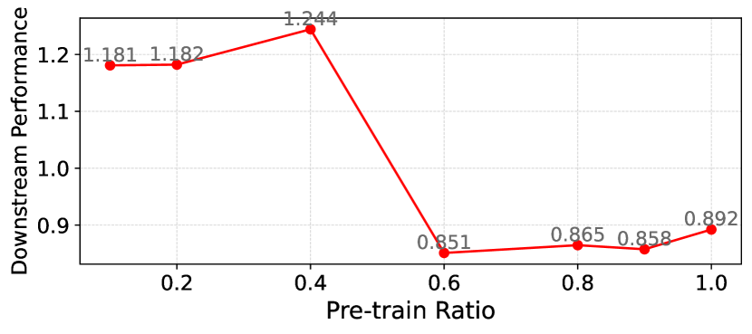
(a) Dengue

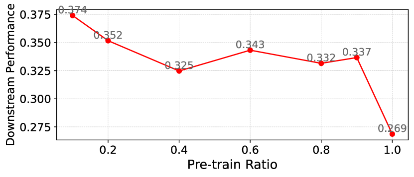
(b) Measles

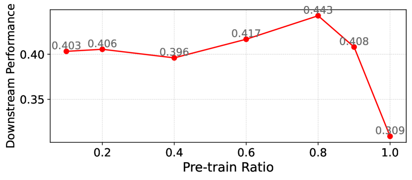
(c) ILI USA

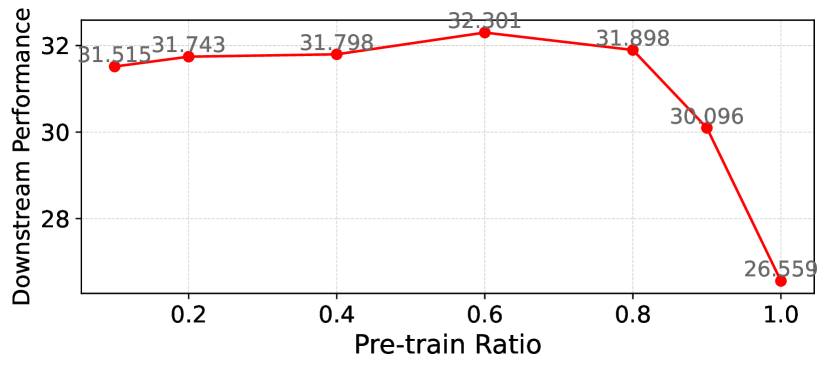
(d) COVID

Figure 9: Downstream performance with different ratios of pre-training datasets. The input length is set to 36 and all MSE results are averaged over {1,2,4,8,16} future steps.

A.7 Visualization of the Estimated Environments

According to $\hat{\mathbf{e}}^{(l)}=\sum_{k=1}^{K}\mathbf{e}_{k}\pi_{k}^{(l)}$, an aggregated environment is the weighted sum of the learned latent environment representations. Therefore, the estimation shares the same latent space as the fixed representations and we are able to visualize them using t-SNE. As shown in Figure 10, we visualize the aggregated environments (Estimated) as well as the learned latent environment (Anchor) from a CAPE model with 8 environments.

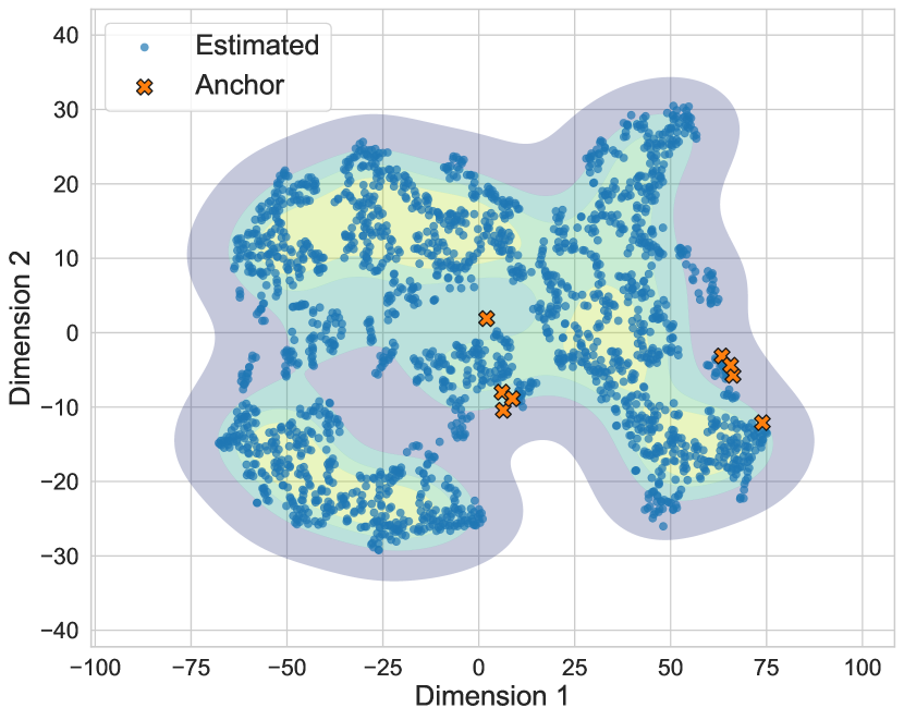
(a) ILI USA

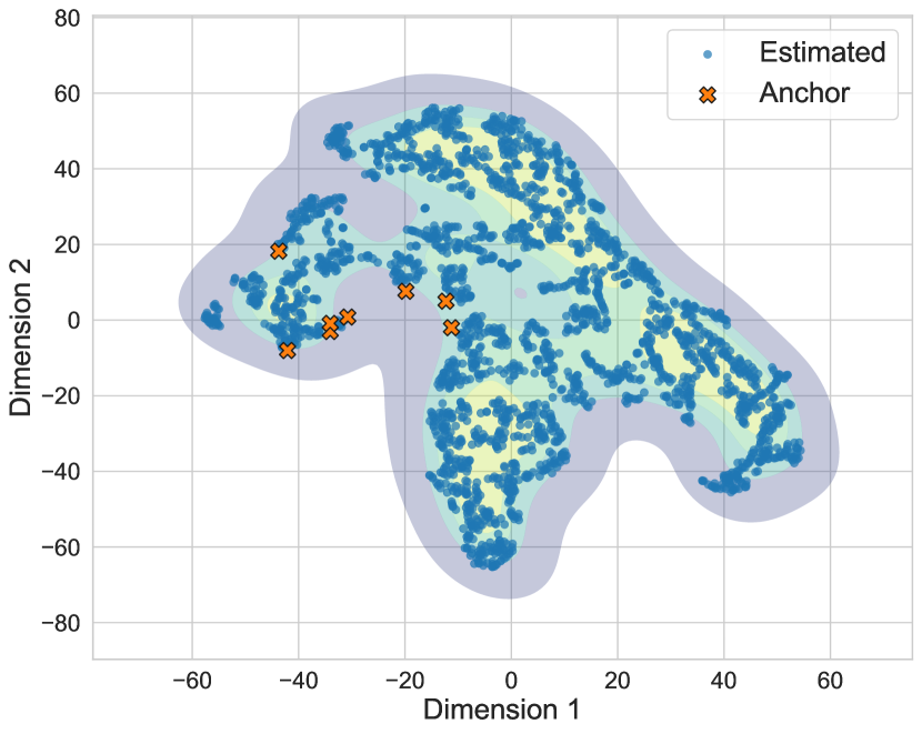
(b) Measles

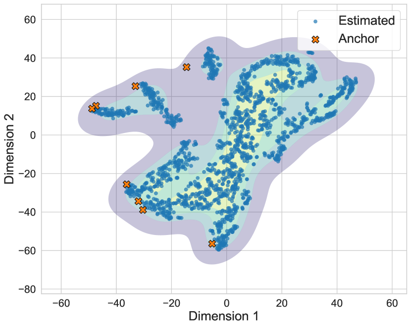
(c) Dengue

Figure 10: Visualization of the estimated environment representations using t-SNE.

A.8 Visualization of Distribution Shift for Downstream Datasets

We provide a visualization of the sample distribution used in this study. Each sample has a fixed length of 36, representing the historical infection trajectory. To better understand the distributional differences, we use t-SNE to reduce the data to one dimension and visualize the training and test samples using different colors. As shown in Figure 11, a significant distribution shift is visually apparent across most datasets. To quantitatively assess the distributional differences between the training and test sets, we calculate the Central Moment Discrepancy (CMD) score Zellinger et al. (2017). The CMD score measures the discrepancy between the central moments of the two distributions up to a specified order $K$. For two distributions $X$ (training set) and $X_{\text{test}}$ (test set), the CMD score is defined as:

$$\quad\text{CMD}(X,X_{\text{test}})$$ (25)

$$=\|\mu_{1}(X)-\mu_{1}(X_{\text{test}})\|_{2}+\sum_{k=2}^{K}\|\mu_{k}(X)-\mu_{k}(X_{\text{test}})\|_{2},$$

where:$\mu_{k}(X)$ denotes the $k$-th central moment of $X$, defined as: $\mu_{k}(X)=\mathbb{E}[(X-\mathbb{E}[X])^{k}],$ and similarly for $\mu_{k}(X_{\text{test}})$. $\|\cdot\|_{2}$ is the Euclidean norm. $K$ is the maximum order of moments considered. The CMD score aggregates the differences in the mean (first moment) and higher-order moments (e.g., variance, skewness), providing a robust measure of the distribution shift. In our experiments, we set $K=3$ to capture up to the third-order central moments. This score quantitatively complements the visual observations in Figure 11, offering a more comprehensive understanding of the distributional differences between training and test sets.

Impact of Distribution Shifts. Distribution shifts between training and test datasets pose significant challenges to the generalizability and robustness of predictive models. When the underlying data distributions differ, models trained on the training set may struggle to maintain their performance on the test set, leading to reduced accuracy and reliability. These discrepancies can arise from various factors, such as temporal changes in infection patterns or geographical variations. In this paper, we assume that the inherent infection pattern of a particular disease remains constant, and the distribution shifts for the disease are primarily caused by the rapidly changing environment, which results in diverse infection patterns. In the context of epidemic modeling, such shifts are especially critical, as they can undermine the model’s ability to accurately predict future infection trends, which is essential for effective public health interventions.

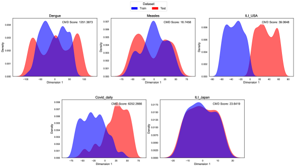
Figure 11: The KDE plot of training set and test set. Each sample contains an infection trajectory of 36 weeks. t-SNE is applied to visualize the distributions of both sets.

A.9 Latent space visualization of Measle and Covid datasets from pre-trained models.

In order to demonstrate that CAPE effectively disentangles the underlying dynamics of diseases from the influence of the environment, we visualize the output embeddings for the Measles and COVID datasets by projecting them into a two-dimensional space using t-SNE. Specifically, we utilize the pre-trained model without fine-tuning on these two downstream datasets and visualize $\mathbf{x}^{(L)}$, the final-layer embeddings, as individual data points in the figure. As shown in Figure 13, CAPE (left) visually separates the two datasets more effectively than the pre-trained PatchTST model (right). To quantitatively evaluate the separability of the embeddings, we compute the Davies–Bouldin Index (DBI), which is defined as:

$$\text{DBI}=\frac{1}{K}\sum_{i=1}^{K}\max_{j\neq i}\left(\frac{\sigma_{i}+\sigma_{j}}{\|\mu_{i}-\mu_{j}\|}\right),$$ (26)

where $K$ is the number of clusters (in this case, two: Measles and COVID), $\mu_{i}$ is the centroid of cluster $i$, $\sigma_{i}$ is the average intra-cluster distance for cluster $i$, defined as: $\sigma_{i}=\frac{1}{|C_{i}|}\sum_{\mathbf{x}\in C_{i}}\|\mathbf{x}-\mu_{i}\|$, where $C_{i}$ is the set of points in cluster $i$, $\|\mu_{i}-\mu_{j}\|$ is the Euclidean distance between the centroids of clusters $i$ and $j$. The DBI measures the ratio of intra-cluster dispersion to inter-cluster separation. Lower DBI values indicate better separability. As shown in Figure 13, CAPE achieves a significantly lower DBI compared to PatchTST, confirming its superior ability to disentangle the underlying disease dynamics from environmental factors. A more complete result is shown in Figure 7.

A.10 Hyper-parameter Sensitivity Analysis

While we treat $\hat{\mathbf{E}}_{j,c}^{(l)}=\hat{\mathbf{e}}^{(l)}_{c}\odot\mathbf{h}^{(l)}_{c}$ in the contrastive loss and aligned the combined representation of the input and environment, we further applied the contrastive loss on the aggregated environment representations at each layer, denoted as $\tilde{{\mathbf{E}}}_{j,c}^{(l)}=\hat{\mathbf{e}}^{(l)}_{c}$ and assigned a hyper-parameter $\beta$ to control for its weight:

$$\mathcal{L}_{\text{final}} =\sum_{\mathbf{x}\in\mathbf{X}}\mathcal{L}_{\text{recon}}(\mathbf{x},\hat{\mathbf{x}})+$$ (27)

$$\alpha\,\mathcal{L}_{\text{CL}}(\hat{\mathbf{E}}^{(L)},\hat{\mathbf{E}^{\prime}}^{(L)})+\frac{\beta}{L}\sum_{l}\mathcal{L}_{\text{CL}}(\tilde{{\mathbf{E}}}^{(l)},\tilde{{\mathbf{E}}^{\prime}}^{(l)}),$$

$$\mathbf{X}\sim\mathcal{D}^{\prime}_{s}\in\mathcal{D}_{\text{pre}}$$

where $L$ denotes the number of layers. Using Equation (27), we further fine-tune our pre-trained model by varying $\alpha$ and $\beta$ across the values [1e-3, 1e-2, 1e-1, 1, 10]. The results of this sensitivity analysis are presented in Figure 12.

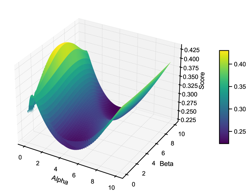
(a) ILI USA

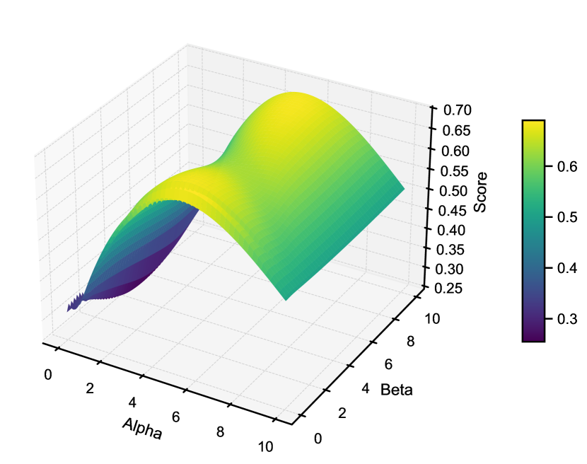
(b) Measles

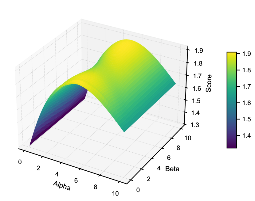
(c) ILI Japan

Figure 12: Hyperparameters sensitivity of $\alpha$ and $\beta$.

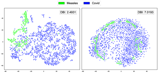
Figure 13: Output latent space of two pre-trained models without fine-tuning from Measle and Covid datasets. Left: CAPE; Right: Pre-trained PatchTST.

References

- Adhikari et al. (2019) Adhikari, B., Xu, X., Ramakrishnan, N., and Prakash, B. A. Epideep: Exploiting embeddings for epidemic forecasting. In Proceedings of the 25th ACM SIGKDD international conference on knowledge discovery & data mining, pp. 577–586, 2019.
- Borghi et al. (2021) Borghi, P. H., Zakordonets, O., and Teixeira, J. P. A covid-19 time series forecasting model based on mlp ann. Procedia Computer Science, 181:940–947, 2021.
- Centers for Disease Control and Prevention (2023a) Centers for Disease Control and Prevention. Influenza-like illness (ili) data - usa. https://gis.cdc.gov/grasp/fluview/fluportaldashboard.html, 2023a.
- Centers for Disease Control and Prevention (2023b) Centers for Disease Control and Prevention. Monkey pox cases data. https://www.cdc.gov/mpox/data-research/cases/index.html, 2023b.
- Centers for Disease Control and Prevention (2023c) Centers for Disease Control and Prevention. Rsv surveillance data. https://www.cdc.gov/rsv/php/surveillance/rsv-net.html, 2023c.
- Chen & Hsieh (2012) Chen, S.-C. and Hsieh, M.-H. Modeling the transmission dynamics of dengue fever: implications of temperature effects. Science of the total environment, 431:385–391, 2012.
- Cooper et al. (2020) Cooper, I., Mondal, A., and Antonopoulos, C. G. A sir model assumption for the spread of covid-19 in different communities. Chaos, Solitons & Fractals, 139:110057, 2020.
- Dong et al. (2020) Dong, E., Du, H., and Gardner, L. An interactive web-based dashboard to track covid-19 in real time. The Lancet infectious diseases, 20(5):533–534, 2020.
- Fraikin et al. (2023) Fraikin, A., Bennetot, A., and Allassonnière, S. T-rep: Representation learning for time series using time-embeddings. arXiv preprint arXiv:2310.04486, 2023.
- Goswami et al. (2024) Goswami, M., Szafer, K., Choudhry, A., Cai, Y., Li, S., and Dubrawski, A. Moment: A family of open time-series foundation models. arXiv preprint arXiv:2402.03885, 2024.
- He et al. (2020) He, S., Peng, Y., and Sun, K. Seir modeling of the covid-19 and its dynamics. Nonlinear dynamics, 101:1667–1680, 2020.
- Jiao et al. (2024) Jiao, L., Wang, Y., Liu, X., Li, L., Liu, F., Ma, W., Guo, Y., Chen, P., Yang, S., and Hou, B. Causal inference meets deep learning: A comprehensive survey. Research, 7:0467, 2024.
- Kamarthi & Prakash (2023) Kamarthi, H. and Prakash, B. A. Pems: Pre-trained epidmic time-series models. arXiv preprint arXiv:2311.07841, 2023.
- Kontopoulou et al. (2023) Kontopoulou, V. I., Panagopoulos, A. D., Kakkos, I., and Matsopoulos, G. K. A review of arima vs. machine learning approaches for time series forecasting in data driven networks. Future Internet, 15(8):255, 2023.
- Lau et al. (2020a) Lau, M. S., Becker, A. D., Korevaar, H. M., Caudron, Q., Shaw, D. J., Metcalf, C. J. E., Bjørnstad, O. N., and Grenfell, B. T. A competing-risks model explains hierarchical spatial coupling of measles epidemics en route to national elimination. Nature Ecology & Evolution, 4(7):934–939, 2020a.
- Lau et al. (2020b) Lau, M. S., Grenfell, B., Thomas, M., Bryan, M., Nelson, K., and Lopman, B. Characterizing superspreading events and age-specific infectiousness of sars-cov-2 transmission in georgia, usa. Proceedings of the National Academy of Sciences, 117(36):22430–22435, 2020b.
- Liang et al. (2024) Liang, Y., Wen, H., Nie, Y., Jiang, Y., Jin, M., Song, D., Pan, S., and Wen, Q. Foundation models for time series analysis: A tutorial and survey. In Proceedings of the 30th ACM SIGKDD Conference on Knowledge Discovery and Data Mining, pp. 6555–6565, 2024.
- Liu et al. (2024a) Liu, Z., Li, Y., Wei, M., Wan, G., Lau, M. S., and Jin, W. Epilearn: A python library for machine learning in epidemic modeling. arXiv preprint arXiv:2406.06016, 2024a.
- Liu et al. (2024b) Liu, Z., Wan, G., Prakash, B. A., Lau, M. S., and Jin, W. A review of graph neural networks in epidemic modeling. In Proceedings of the 30th ACM SIGKDD Conference on Knowledge Discovery and Data Mining, pp. 6577–6587, 2024b.
- Ma et al. (2024) Ma, Q., Liu, Z., Zheng, Z., Huang, Z., Zhu, S., Yu, Z., and Kwok, J. T. A survey on time-series pre-trained models. IEEE Transactions on Knowledge and Data Engineering, 2024.
- Madden et al. (2024) Madden, W. G., Jin, W., Lopman, B., Zufle, A., Dalziel, B., E. Metcalf, C. J., Grenfell, B. T., and Lau, M. S. Deep neural networks for endemic measles dynamics: Comparative analysis and integration with mechanistic models. PLOS Computational Biology, 20(11):e1012616, 2024.
- Mao et al. (2022) Mao, C., Xia, K., Wang, J., Wang, H., Yang, J., Bareinboim, E., and Vondrick, C. Causal transportability for visual recognition. In Proceedings of the IEEE/CVF Conference on Computer Vision and Pattern Recognition, pp. 7521–7531, 2022.
- Natarajan et al. (2023) Natarajan, S., Kumar, M., Gadde, S. K. K., and Venugopal, V. Outbreak prediction of covid-19 using recurrent neural network with gated recurrent units. Materials Today: Proceedings, 80:3433–3437, 2023.
- National Institute of Infectious Diseases (2023) National Institute of Infectious Diseases. Infectious diseases weekly report (idwr) - japan. https://www.niid.go.jp/niid/en/idwr-e.html, 2023.
- Nicola et al. (2020) Nicola, M., Alsafi, Z., Sohrabi, C., Kerwan, A., Al-Jabir, A., Iosifidis, C., Agha, M., and Agha, R. The socio-economic implications of the coronavirus pandemic (covid-19): A review. International journal of surgery, 78:185–193, 2020.
- Nie et al. (2022) Nie, Y., Nguyen, N. H., Sinthong, P., and Kalagnanam, J. A time series is worth 64 words: Long-term forecasting with transformers. arXiv preprint arXiv:2211.14730, 2022.
- OpenDengue (2023) OpenDengue. Dengue data across countries. https://opendengue.org/, 2023.
- Panagopoulos et al. (2021) Panagopoulos, G., Nikolentzos, G., and Vazirgiannis, M. Transfer graph neural networks for pandemic forecasting. In Proceedings of the AAAI Conference on Artificial Intelligence, volume 35, pp. 4838–4845, 2021.
- Rasul et al. (2023) Rasul, K., Ashok, A., Williams, A. R., Khorasani, A., Adamopoulos, G., Bhagwatkar, R., Biloš, M., Ghonia, H., Hassen, N., Schneider, A., et al. Lag-llama: Towards foundation models for time series forecasting. In R0-FoMo: Robustness of Few-shot and Zero-shot Learning in Large Foundation Models, 2023.
- Runge et al. (2023) Runge, J., Gerhardus, A., Varando, G., Eyring, V., and Camps-Valls, G. Causal inference for time series. Nature Reviews Earth & Environment, 4(7):487–505, 2023.
- Sahai et al. (2020) Sahai, A. K., Rath, N., Sood, V., and Singh, M. P. Arima modelling & forecasting of covid-19 in top five affected countries. Diabetes & metabolic syndrome: clinical research & reviews, 14(5):1419–1427, 2020.
- Shahid et al. (2020) Shahid, F., Zameer, A., and Muneeb, M. Predictions for covid-19 with deep learning models of lstm, gru and bi-lstm. Chaos, Solitons & Fractals, 140:110212, 2020.
- Shang et al. (2021) Shang, A. C., Galow, K. E., and Galow, G. G. Regional forecasting of covid-19 caseload by non-parametric regression: a var epidemiological model. AIMS public health, 8(1):124, 2021.
- (34) Sun, S. et al. Caudits: Causal disentangled domain adaptation of multivariate time series. In Forty-first International Conference on Machine Learning.
- van Panhuis et al. (2018) van Panhuis, W. G., Cross, A., and Burke, D. S. Project tycho 2.0: a repository to improve the integration and reuse of data for global population health. Journal of the American Medical Informatics Association, 25(12):1608–1617, 2018.
- Wan et al. (2024) Wan, G., Liu, Z., Lau, M. S., Prakash, B. A., and Jin, W. Epidemiology-aware neural ode with continuous disease transmission graph. arXiv preprint arXiv:2410.00049, 2024.
- Wang et al. (2020) Wang, P., Zheng, X., Ai, G., Liu, D., and Zhu, B. Time series prediction for the epidemic trends of covid-19 using the improved lstm deep learning method: Case studies in russia, peru and iran. Chaos, Solitons & Fractals, 140:110214, 2020.
- Wang et al. (2024a) Wang, Y., Wu, H., Dong, J., Liu, Y., Long, M., and Wang, J. Deep time series models: A comprehensive survey and benchmark. arXiv preprint arXiv:2407.13278, 2024a.
- Wang et al. (2024b) Wang, Y., Wu, H., Dong, J., Liu, Y., Long, M., and Wang, J. Deep time series models: A comprehensive survey and benchmark. 2024b.
- Wu et al. (2021) Wu, H., Xu, J., Wang, J., and Long, M. Autoformer: Decomposition transformers with auto-correlation for long-term series forecasting. Advances in neural information processing systems, 34:22419–22430, 2021.
- Wu et al. (2023) Wu, H., Hu, T., Liu, Y., Zhou, H., Wang, J., and Long, M. Timesnet: Temporal 2d-variation modeling for general time series analysis. In International Conference on Learning Representations, 2023.
- Yue et al. (2022) Yue, Z., Wang, Y., Duan, J., Yang, T., Huang, C., Tong, Y., and Xu, B. Ts2vec: Towards universal representation of time series. In Proceedings of the AAAI Conference on Artificial Intelligence, volume 36, pp. 8980–8987, 2022.
- Zellinger et al. (2017) Zellinger, W., Grubinger, T., Lughofer, E., Natschläger, T., and Saminger-Platz, S. Central moment discrepancy (cmd) for domain-invariant representation learning. arXiv preprint arXiv:1702.08811, 2017.
- Zeng et al. (2023) Zeng, A., Chen, M., Zhang, L., and Xu, Q. Are transformers effective for time series forecasting? In Proceedings of the AAAI conference on artificial intelligence, volume 37, pp. 11121–11128, 2023.
- Zerveas et al. (2021) Zerveas, G., Jayaraman, S., Patel, D., Bhamidipaty, A., and Eickhoff, C. A transformer-based framework for multivariate time series representation learning. In Proceedings of the 27th ACM SIGKDD conference on knowledge discovery & data mining, pp. 2114–2124, 2021.
- Zhang et al. (2022) Zhang, X., Zhao, Z., Tsiligkaridis, T., and Zitnik, M. Self-supervised contrastive pre-training for time series via time-frequency consistency. Advances in Neural Information Processing Systems, 35:3988–4003, 2022.
- Zhao et al. (2023) Zhao, W. X., Zhou, K., Li, J., Tang, T., Wang, X., Hou, Y., Min, Y., Zhang, B., Zhang, J., Dong, Z., et al. A survey of large language models. arXiv preprint arXiv:2303.18223, 2023.
- Zhou et al. (2023) Zhou, F., Mao, Y., Yu, L., Yang, Y., and Zhong, T. Causal-debias: Unifying debiasing in pretrained language models and fine-tuning via causal invariant learning. In Proceedings of the 61st Annual Meeting of the Association for Computational Linguistics (Volume 1: Long Papers), pp. 4227–4241, 2023.
- Zhou et al. (2021) Zhou, H., Zhang, S., Peng, J., Zhang, S., Li, J., Xiong, H., and Zhang, W. Informer: Beyond efficient transformer for long sequence time-series forecasting. In Proceedings of the AAAI conference on artificial intelligence, volume 35, pp. 11106–11115, 2021.
- Zhou et al. (2022) Zhou, T., Ma, Z., Wen, Q., Wang, X., Sun, L., and Jin, R. Fedformer: Frequency enhanced decomposed transformer for long-term series forecasting. In International conference on machine learning, pp. 27268–27286. PMLR, 2022.