On the Conditional Phase Distribution of the TWDP Multipath Fading Process
Abstract
In this paper, the conditional phase distribution of the two-wave with diffuse power (TWDP) process is derived as a closed-form and as an infinite-series expression. For the obtained infinite series expression, a truncation analysis is performed and the truncated expression is used to examine the influence of different channel conditions on the behavior of the TWDP phase. All the results are verified through Monte Carlo simulations.
Index Terms:
conditional phase distribution, mmWave band, TWDP multipath fadingI Introduction
Two-wave with diffuse power (TWDP) is a multipath fading model introduced to model better-than-Rayleigh and worse-than-Rayleigh fading conditions [8]. The model has been empirically verified in vehicular-to-infrastructure (V2I), vehicle-to-vehicle (V2V) and indoor propagation environments at 60 GHz, as well as in wireless sensor networks deployed in cavity environments [21, 27, 26, 10]. It also incorporates Rayleigh and Rician models as special cases, which makes it applicable for modeling multipath fading in various propagation scenarios encountered in the emerging wireless networks.
Given its significance, TWDP envelope statistics have been studied extensively [8, 19, 13]. However, characteristics of the received signal envelope reveal only part of the overall channel picture [5]. Therefore, to fully characterize the fading process, the statistical properties of the corresponding phase are also of interest, since they can be used in the design and synchronization of coherent receivers and in the detection of M-ary phase shift keying signal constellations [5]. More precisely, the knowledge about the phase behavior can be utilized for the optimal design and synchronization of coherent receivers, where carrier recovery schemes are required [18]. Additionally, the performance of modulation systems using non-ideal coherent or incoherent detection, as well as those employing an orthogonal frequency-division multiple access (OFDM) modulation scheme, is also affected by the phase statistics of the communication channel [18]. Accordingly, understanding the properties of the phase distribution is essential for the design of wireless systems [4].
However, despite its importance, and the fact that the probability distribution function (PDF) of the phase process has been derived and discussed for many multipath fading models (such as Rician [23], Nakagami-m [15, 25], [3], [18], etc.), no results regarding the phase behavior have been provided for the TWDP model. The only relevant results are published in [11], where the phase probability density function of the sum of the signal, noise and cochannel interference is considered under equivalent statistical assumptions to those of the TWDP model [13].
In this paper, we derived the conditional PDF of the TWDP phase stemming from the fundamental underlying assumptions of the TWDP model itself, and then, investigated the impact of different multipath fading conditions on the behavior of the phase process. Accordingly, after the Introduction given in Section I, the conditional TWDP phase PDF is foremost derived as an infinite-series expression in Section II. This is followed by an appropriate truncation analysis, given in Section IV, and derivation of the closed-form expression in Section III. Numerical results, presented in Section V, verified the obtained analytical results, providing for the first time in the literature, insight into the behavior of the TWDP phase process and its specific features. The derived analytical expressions are also verified using the developed TWDP geometrically-based simulator in Section VI, and the results are finally applied to error performance evaluation in Section VII. Final conclusions and guidelines for future work are given in Section VII.
II Conditional TWDP Phase PDF
TWDP is a multipath fading model applicable for modeling various fading conditions. It assumes that the complex envelope of the signal propagating in the TWDP channel is composed of two strong specular components and , along with the diffuse component [8]:
| (1) |
It also assumes that the specular components have constant magnitudes , , where , and uniformly distributed phases , in the range , while the diffuse component is considered as a zero mean Gaussian random process with average power .
To derive the conditional PDF of the TWDP phase, when the stronger specular component is ideally recovered, without loss of generality can be assumed that 111 To simplify the notation, the condition is not explicitly stated in the remaining text.. In this case, the conditional complex TWDP envelope can be expressed as the sum of and the Rician component , as shown in Fig. 1:
| (2) |
Following the aforesaid and the phasor diagram given in Fig. 1, the conditional distribution of the TWDP phase, , can be obtained using one of the following expressions:
-
1.
(3) -
2.
(4)
The first approach is employed in [12], where the conditional phase is derived for the sum of signal, cochannel interference and AWGN. It is shown that this phase follows the same statistical characteristics as the components of the TWDP model itself. However, the conditional PDF of the phase derived in [12] is given in the Fourier series form which involves several sums and consequently has a quite complex mathematical notation.
Accordingly, to obtain more analytically tractable expression, this paper employs the second approach which first requires derivation of the conditional distribution , where is the envelope of the Rician-distributed variable. To achieve this, we started from the joint envelope-phase PDF of the Rician component, given as [4]:
| (5) |
where, by definition, the angle is uniformly distributed i.e., , and is the Rician phase PDF (as can be seen in Fig. 1). Consequently, it can be shown that is uniformly distributed between and , i.e., .
Since is invariant with respect to the arbitrary angular shift, i.e., , it can be shown that for , is equal to . Under this condition and after some manipulations of (5), it can be concluded that and are mutually independent, with the corresponding PDFs given as:
| (6) |
| (7) |
or alternatively, as [1, 03.02.02.0001.01]:
| (8) |
Considering the above, can be derived from given in (6) by applying a random variable transformation:
| (9) |
as:
| (10) |
and the conditional PDF of the TWDP phase can be obtained after inserting (10) and (8) into (4), as:
| (11) |
| (12) |
Note that after some manipulations, both equations, (11) and (12), can be merged into the single expression and expressed as a sum of three different integrals:
| (13) |
where these integrals are defined and solved respectively, as:
| (14) |
| (15) |
| (16) |
| (17) | ||||
| (18) | ||||
As a result, the final expression for the conditional phase PDF of the TWDP multipath fading process is given by (17), where is the Tricomi confluent hypergeometric function and is the Humbert confluent hypergeometric function (both of which can be easily evaluated and efficiently implemented in most standard software packages, such as Matlab and Mathematica), while the general expression for the arbitrary phase of the stronger specular component is given by (18).
Since TWDP model includes the Rice () and Rayleigh () models as special cases, the correctness of (18) can be confirmed by its reduction to these well-known phase PDFs. Specifically, for , only the first summation term (i.e. ) exists in (18), so according to [1, 07.33.03.0005.01], and [6, 4.18], [1, 07.20.17.0013.01], [1, 06.25.26.0001.01], equation (18) reduces to the well-known form of the Rician phase PDF [2, eq. (45)]. The conditional probability density function of the Rician PDF further reduces to when the dominant specular component vanishes (), as expected for Rayleigh fading.
III Closed-form expression
In this section, the closed-form expression for the conditional TWDP phase PDF is derived, starting from its infinite series representation given by (18). To obtain it’s closed-form counterpart, expression (18) is treated as the sum of three separated series.
To solve the first series, [1, 07.33.03.0014.01] and [1, 06.06.07.0001.01] are used, and the order of integration and summation is reversed. The resulting sum and integral are then solved with the help of [1, 03.02.02.0001.01], and [6, eq. (3.12)], respectively, and expressed in terms of the Humbert confluent hypergeometric function .
The second series is solved with the help of [1, 07.33.17.0007.01], [1, 07.33.03.0052.01], and [16, eq. (5.11.4.11)], and is also expressed in terms of the function.
The third series is then solved using [22, Sec. 1.6 eq. (36)] and [22, Sec. 1.7 eq. (39)], and the final closed-form expression of the conditional TWDP phase is given by (19), where is the general triple hypergeometric function.
| (19) | ||||
Accordingly, the closed form of the conditional TWDP phase PDF involves Humbert confluent and general triple hypergeometric functions, which are less known and relatively complex. Therefore, it is necessary to investigate the convergence of (19), which can be easily proven with the help of [20, p. 28]:
| (20) |
and [22, Sec. 1.7 eq. (41)].
Despite that, its practical implementation and interpretation of its results are complex. Therefore, in the following section, a truncation analysis of the infinite series representation of the conditional TWDP phase PDF, given in (17) or (18), is provided and the obtained expression is used for all subsequent analysis.
IV Truncation Error of the Infinite-series Expression
The truncated sum, as a method, reduces the complexity of the analysis and data processing, making them more appropriate for practical application. This approach not only simplifies the calculations, but also enhances the model’s robustness, allowing better interpretation of the results. Below, the truncation error analysis is presented, followed by concrete examples to illustrate its application.
Since the conditional PDF of the TWDP phase (17) is expressed as an infinite-series, it is essential to determine the finite number of summation terms to achieve the desired truncation error. Therefore, let’s begin with the initial integral expression (4):
| (21) |
where , according to (8), can be expressed in series form as:
| (22) |
where the conditional random variable follows a Nakagami-m distribution, i.e.
Nakagami-m(,), while is a Poisson distributed random variable, i.e. .
Accordingly, the conditional PDF of the TWDP phase is obtained as the following series:
| (23) |
where is determined in its exact form, as given (see (17)). Consequently, the truncation error of the conditional phase PDF will be directly dependent on the truncation error of . So, to assess the truncation error of the distribution , let’s adopt the measure that % of the total average power of the variable is preserved in the truncated sum. To satisfy this requirement, the total average power of the variable can be expressed as:
| (24) |
which, after the total average power normalization, allows us to calculate the share of the total average power over the particular summation terms as:
| (25) |
Since is obviously normalized, it represents PDF of the average power over the summation terms, given as:
| (26) |
which can be written as:
| (27) |
where and . Clearly, the amount of average power across the summation terms follows a weighted Poisson distribution. Thus, the boundaries of the summation terms, which preserve % of the total average power of the variable , can be determined as the % confidence interval of the average power distribution over these summation terms.
Considering the aforesaid, the confidence interval of the weighted Poisson distribution can be determined as the subset of the union of the confidence intervals of each individual Poisson variable:
| (28) |
where Wald’s confidence interval [14] for each variable can be obtained as:
| (29) |
and
| (30) |
Accordingly, the boundaries of the truncated sum, which preserve at least of the total average power of random variable , can be determined as:
| (31) |
i.e.
| (32) |
Considering the aforementioned, the truncated conditional TWDP phase PDF, which preserves 99.9% of the total average power, can be calculated using the following expression:
| (33) |
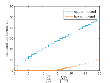
Fig. 3 shows the upper and the lower bounds of the summation terms given by (33), which must be considered to achieve defined truncation error in terms of . These bounds are also expressed in terms of the TWDP model’s parameters , , and , defined as [13]: , for , and , as these parameters can be more easily correlated with different channel conditions.
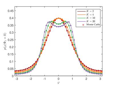
As it can be observed from Fig. 3, the derived phase PDF expression converges very quickly, especially for small values of and . Also, even for very large values of these parameters (e.g. when and ) the number of summation terms required to preserve 99.9% of the total average power remains relatively low (only 40, ranging from 10 to 49). Accordingly, the summation terms determined in (33) are used for all calculations of the conditional PDF of the TWDP phase, , in the following sections.
V Numerical results
In this section, obtained analytical results are plotted to demonstrate the influence of different channel conditions on the behavior of the conditional TWDP phase. The validity of the derived expression (17) is also examined, by comparing theoretical curves against simulated results, which are generated using Monte Carlo simulation and samples. As shown in Fig. LABEL:Fig1 - Fig. LABEL:Fig4, there is an excellent match between simulation and analytical results for all considered cases.
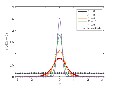
In the initial step, the conditional TWDP phase PDF for Rician fading channel conditions is plotted in Fig. LABEL:Fig1 by setting (which occurs when only one specular component is present) and varying the values of , in order to provide the reference point for further examination. The figure shows that for (i.e. when both specular components are absent and only diffuse component exists), the conditional phase follows an uniform distribution, as expected in Rayleigh channel. For other values of , the obtained PDFs exhibit a symmetrical Gaussian-like shape, typical of Rician fading. In these cases, the phase variance decreases as increases, and the distribution can be well approximated by the Tikhonov (von Mises) PDF.
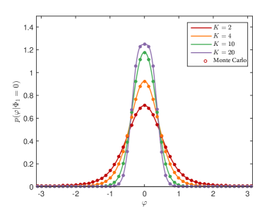
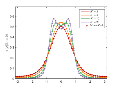
Figures LABEL:Fig2–LABEL:Fig4 illustrate other cases typical for channels with TWDP fading. These figures demonstrate that the appearance of the second specular component changes the phase PDF shape, simultaneously increasing its variance compared to the Rician case. These figures also show that the observed variance’s increment becomes more pronounced for larger values of , i.e., as the magnitude of the second specular component increases. More specifically, for small values of or small values of , which describe better-than-Rayleigh fading conditions [13] (where the observed fading is less severe than in Rayleigh channels [13]), the conditional TWDP phase PDF exhibits a Gaussian-like unimodal shape with even symmetry. This behavior is similar to that observed in Rician fading channels, suggesting that any topic related to the phase estimation can be treated in a similar manner to Rician channels.
However, as both and increase (i.e. when the power of two specular components are similar and significantly larger than the power of the diffuse component), the phase PDF becomes bimodal. It is shown in [13] that such combination of parameters corresponds to a very severe fading, which is classified as worse-than-Rayleigh. Accordingly, in channels with worse-than-Rayleigh fading, the phase PDF is spread out and exhibits bimodal behavior. In such cases, it is necessary to examine the phase error behavior obtained within the synchronization procedure, which is going to be significantly different from that observed in Rician channels.
VI Verification of the Derived Analytical Expressions
In this section, we verified theoretically obtained results using developed geometrically-based simulator which reflects propagation conditions in TWDP channel. To achieve this, propagation environment is constructed to closely align with the theoretical assumptions. It is assumed that the stronger specular component arrives to the receiver with constant envelope and constant phase , while the weaker specular component propagates to the receiver with constant envelope and random phase . It is also assumed that the diffuse component results from the isotropic 2-D scattering, as Clarke suggested in [7].
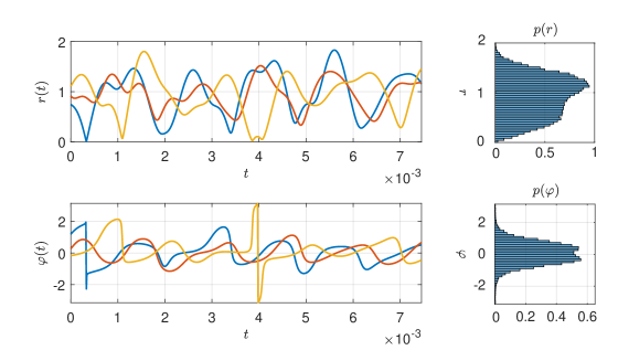
The propagation environment supporting these theoretical assumptions is constructed as below. The transmitter is fixed at the coordinates (0, 5 m), while the receiver, positioned at the origin of the global coordinate system, moves with a constant velocity =10 m/s in the direction of the x-axis. The reflective plane is placed in the receiver’s vicinity at coordinates (3.6633 m, -4.0613 m), at an angle of 25.0244∘. When signal is emitted, the stronger specular component propagates along the line-of-sight (LoS) between the transmitter and the receiver and arrives perpendicular to the direction of motion. As such, a total phase of the stronger specular component is almost unaffected by the Doppler effect. On the other hand, the azimuthal angle of arrival of the weaker specular component, determined by relative positions of the receiver, transmitter and reflector, causes its total phase to change much faster than the phase of the stronger specular component. Considering the aforesaid, simulation time is set to 7.510-3s, in which LOS component rotates for 10∘, while the weaker specular component makes 5 full rotations. In addition, the maximum Doppler frequency is set to 1000 Hz, which corresponds to the carrier frequency of 30 GHz for a chosen velocity. The sample time is chosen in way that , i.e., sample time is set to s. On the other side, diffuse component is simulated as described in [24]. To average the effect of diffuse component on the overall phase distribution, different realizations are taken into consideration, and used to obtain histograms given in Fig. 5 and Fig. 6.
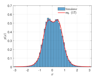
Three different realizations of the amplitude and the phase of the TWDP process are obtained using described simulator and illustrated in Fig. 5, together with corresponding histograms which exhibit expected bimodal behavior. In Fig. 6, TWDP phase histogram obtained by the simulator is compared to the derived analytical phase PDF (17), showing an excellent match between them, thus providing additional verification of the derived expressions.
VII Performance Analysis
To demonstrate the applicability of the derived phase PDF, the error probability (), introduced in [4], is determined for the -ary Phase Shift Keying (PSK) modulation scheme. Considered error probability, , caused by imperfect phase synchronization without considering impact of the white Gaussian noise, is defined as [4]:
| (34) |
where is the modulation order and is the phase PDF. Considering the aforesaid, for TWDP channel can be obtained by inserting (17) into (34). Unfortunately, due to the complexity of the integral, given expression is evaluated numerically and the results are presented in Fig. LABEL:Fig11 - Fig. LABEL:Fig22, together with those obtained using Monte Carlo simulation, which are in perfect accordance with analytical results.
The results indicate that for higher modulation orders the parameter has a negligible impact on , where is high regardless of the value of (i.e. the severity of fading). In contrast, for BPSK modulation, as the parameter increases (i.e. as fading severity decreases), the error probability decreases significantly.
A similar conclusion can be drawn from Fig. LABEL:Fig22, obtained for BPSK modulation scheme exclusively. Obviously, in channels in which multipath fading is not particularly severe (), changes as a function of channel conditions (i.e. specific values of and ). In contrast, for channels with the pronounced multipath fading (), the values of are very high and are minimally influenced by the change of .
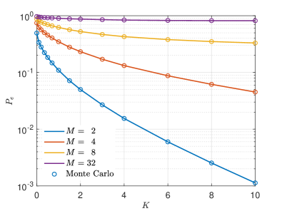
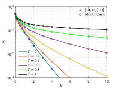
The Fig. LABEL:Fig22 is additionally important since one of the curves, obtained for , can be compared with the results provided in [4]. To facilitate this comparison, the limiting expression of derived for a composite Rician-Rician channel in [4, eq. (11)] is plotted for no-shadowing case (for ). This curve (represented by asterisks) illustrates the behavior of in Rician channels and clearly matches the results obtained by combining equations (34) and (17) for , which once again validates the accuracy of the derived analytical expressions.
VIII Conclusion
In this paper, the exact closed-form and the infinite-series expressions for the conditional TWDP phase PDF are derived and used to investigate the impact of various propagation conditions on the behavior of the corresponding phase process. It is shown that, under better-than-Rayleigh fading conditions, the conditional phase PDF is unimodal, similar to the behavior observed in Rician channels. In such cases, the performance of modulation systems with non-ideal coherent detection can be assessed using already known principles. On the contrary, with the deterioration of fading conditions, the phase PDF becomes bimodal and spreads over the wider range of phase values . Therefore, under these conditions, all aspects related to phase estimation, need to be reconsidered.
Acknowledgment
The authors would like to thank Prof. Ivo Kostić for many valuable discussions and advice. Also, the authors are greatly thankful to Prof. Nikolay Savischenko for his help in obtaining closed-form expressions.
References
- [1] Wolfram functions. https://functions.wolfram.com/.
- Beckmann [1964] Petr Beckmann. Rayleigh distribution and its generalizations. Radio Sci. J. Res. NBS/USNC-URSI, 68(9):927–932, 1964.
- Benevides da Costa and Yacoub [2007] Daniel Benevides da Costa and Michel Daoud Yacoub. The - joint phase-envelope distribution. IEEE Antennas and Wireless Propagation Letters, 6:195–198, 2007. doi: 10.1109/LAWP.2007.895919.
- Browning et al. [2019] Jonathan W. Browning, Simon L. Cotton, David Morales-Jimenez, and F. Javier Lopez-Martinez. The rician complex envelope under line of sight shadowing. IEEE Communications Letters, 23(12):2182–2186, 2019. doi: 10.1109/LCOMM.2019.2939304.
- Browning et al. [2023] Jonathan W. Browning, Simon L. Cotton, Paschalis C. Sofotasios, David Morales-Jimenez, and Michel Daoud Yacoub. A unification of los, non-los, and quasi-los signal propagation in wireless channels. IEEE Transactions on Antennas and Propagation, 71(3):2682–2696, 2023. doi: 10.1109/TAP.2022.3231686.
- Brychkov and Saad [2012] Yu. A. Brychkov and Nasser Saad. Some formulas for the Appell function F1(a,b,b’;c;w,z). Integral Transforms and Special Functions, 23(11):793–802, 2012. doi: 10.1080/10652469.2011.636651.
- Clarke [1968] R. H. Clarke. A statistical theory of mobile-radio reception. The Bell System Technical Journal, 47(6):957–1000, 1968. doi: 10.1002/j.1538-7305.1968.tb00069.x.
- Durgin et al. [2002] G. D. Durgin, T. S. Rappaport, and D. A. de Wolf. New analytical models and probability density functions for fading in wireless communications. IEEE Transactions on Communications, 50(6):1005–1015, 2002.
- Erdélyi [1940] A. Erdélyi. Some Confluent Hypergeometric Functions of Two Variables. Proceedings of the Royal Society of Edinburgh, 60(3):344–361, 1940. doi: 10.1017/S0370164600020307.
- Frolik [2008] J. Frolik. On appropriate models for characterizing hyper-Rayleigh fading. IEEE Transactions on Wireless Communications, 7(12):5202–5207, 2008.
- Kostic [1982] I. Kostic. Error rates of dcpsk signlas in hard-limited multilink systems with cochannel interference and noise. IEEE Transactions on Communications, 30(1):222–230, 1982. doi: 10.1109/TCOM.1982.1095359.
- Kostic [1979] I.M. Kostic. Fourier-series representation for phase density of sum of signal, noise and interference. Electronics Letters, 15:541–542(1), August 1979. ISSN 0013-5194.
- Maric et al. [2021] Almir Maric, Enio Kaljic, and Pamela Njemcevic. An alternative statistical characterization of TWDP fading model. Sensors, 21(22):7513, 2021.
- Patil and Kulkarni [2012] V.V. Patil and H.V. Kulkarni. Comparison of confidence intervals for the poisson mean: Some new aspects. REVSTAT-Statistical Journal, 10(2):211–22, Jul. 2012. doi: 10.57805/revstat.v10i2.117.
- Porto et al. [2013] Iury B. G. Porto, Michel D. Yacoub, Jose Candido S. Santos Filho, Simon L. Cotton, and William G. Scanlon. Nakagami-m phase model: Further results and validation. IEEE Wireless Communications Letters, 2(5):523–526, 2013. doi: 10.1109/WCL.2013.070113.130327.
- Prudnikov et al. [1986a] A. P. Prudnikov, Yu. A. Bryčkov, and O. I. Maričev. Integrals and Series Vol II: Special Functions. Gordon and Breach Science Publishers, 1986a.
- Prudnikov et al. [1986b] A. P. Prudnikov, Yu. A. Bryčkov, and O. I. Maričev. Integrals and Series Vol I: Elementary Functions. Gordon and Breach Science Publishers, 1986b.
- Pôrto and Yacoub [2016] Iury Bertollo Gomes Pôrto and Michel Doud Yacoub. On the phase statistics of the - process. IEEE Transactions on Wireless Communications, 15(7):4732–4744, 2016. doi: 10.1109/TWC.2016.2544924.
- Rao et al. [2015] M. Rao, F. J. Lopez-Martinez, M. Alouini, and A. Goldsmith. MGF approach to the analysis of generalized two-ray fading models. IEEE Transactions on Wireless Communications, 14(5):2548–2561, 2015.
- Ribeiro [2024] Pedro Ribeiro. Humbert functions and sums of squares (slides). In Hypergeometric and Orthogonal Polynomials Event (HOPE), Nijmegen (Netherlands), May 1-3, 2024.
- Schwarz et al. [2020] Stefan Schwarz, Erich Zöchmann, Martin Müller, and Ke Guan. Dependability of directional millimeter wave vehicle-to-infrastructure communications. IEEE Access, 8:53162–53171, 2020. doi: 10.1109/ACCESS.2020.2981166.
- Srivastava and Manocha [1984] H. M. Srivastava and H. L. Manocha. A Treatise on Generating Functions. Ellis Horwood Limited, 1984. ISBN 0-85312-508-2.
- Tikhonov and Kulman [1975] V. I. Tikhonov and N. K. Kulman. Non-linear Filtering and Quasi-Coherent Signals Reception. Sov. Radio. Moscow, 1975.
- Xiao et al. [2006] Chengshan Xiao, Yahong Rosa Zheng, and Norman C. Beaulieu. Novel sum-of-sinusoids simulation models for rayleigh and rician fading channels. IEEE Transactions on Wireless Communications, 5(12):3667–3679, 2006. doi: 10.1109/TWC.2006.256990.
- Yacoub [2010] Michel Daoud Yacoub. Nakagami- phase–envelope joint distribution: A new model. IEEE Transactions on Vehicular Technology, 59(3):1552–1557, 2010. doi: 10.1109/TVT.2010.2040641.
- Zöchmann et al. [2019] Erich Zöchmann, Sebastian Caban, Christoph F. Mecklenbräuker, Stefan Pratschner, Martin Lerch, Stefan Schwarz, and Markus Rupp. Better than Rician: Modelling millimetre wave channels as two-wave with diffuse power. EURASIP Journal on Wireless Communications and Networking, 2019(1), January 2019. doi: 10.1186/s13638-018-1336-6.
- Zöchmann et al. [2019] Erich Zöchmann, Markus Hofer, Martin Lerch, Stefan Pratschner, Laura Bernadó, Jiri Blumenstein, Sebastian Caban, Seun Sangodoyin, Herbert Groll, Thomas Zemen, Aleš Prokeš, Markus Rupp, Andreas F. Molisch, and Christoph F. Mecklenbräuker. Position-specific statistics of 60 ghz vehicular channels during overtaking. IEEE Access, 7:14216–14232, 2019.