1 Detailed Regret Analysis

We consider the regret of round $t$ under four cases when the user provides negative feedback to the visualization:

1. Like configuration $c_{t}$ and attribute pair $\{x_{t},y_{t}\}$

2. Like attribute pair $\{x_{t},y_{t}\}$ but not configuration $c_{t}$

3. Like configuration $c_{t}$ but not attribute pair $\{x_{t},y_{t}\}$

4. Dislike configuration $c_{t}$ and attribute pair $\{x_{t},y_{t}\}$

For case (1), we provide the regret bound by analyzing the bias term converges in certain rounds.

Lemma 1.

The reward gap between optimal and sub-optimal bias $\gamma$ is bounded with the overall round $T$ and the time $t_{\gamma}$ that $\gamma$ has been played for.

$$\Delta_{\gamma}\leq\sqrt{\frac{ln(T)}{t_{\gamma}}}$$ (1)

Proof.

having a positive configuration and attributes while negative visualization implies:

$$U(c,a)\geq U(c^{\ast},a^{\ast})$$ (2)

where $c^{\ast},a^{\ast}$ refers to configuration and attributes of preferred visualization. Notably, $c,a$ may also receive positive feedback from user, but their combination is not preferred. In this case, $\Delta_{c}=\Delta_{a}=0$ and we bound the regret with bias.

$$\Delta_{bias}\leq\rho_{c,t}+\rho_{a,t}+\rho_{\gamma,t}-\rho_{c,t}^{\ast}-\rho_{a,t}^{\ast}-\rho_{t,\gamma}^{\ast}$$ (3)

The round that $\gamma^{\ast}$ is updated given $c,a$ should be less than either $t_{a}^{\ast}$ or $t_{c}^{\ast}$, we define $t_{max}^{\ast}=max(t_{a}^{\ast},t_{c}^{\ast})\geq t_{min}^{\ast}=min(t_{a}^{\ast},t_{c}^{\ast})\geq t_{\gamma}^{\ast}$. Using the definition of UCB, we can bound the gap of bias by

$$\Delta_{bias} \leq 3\sqrt{\frac{2ln(T)}{t_{\gamma}}}-3\sqrt{\frac{2ln(T)}{t^{\ast}_{max}}}\leq 3\sqrt{\frac{2ln(T)}{t_{\gamma}}}$$ (4)

$$t_{\gamma} \leq 18ln(T)\frac{1}{\Delta_{bias}^{2}}$$ (5)

∎

With 1, we can bound the regret bound of case (1) by:

$$Reg_{1}=\mathbb{E}[t_{\gamma}]\Delta_{bias}\leq 18ln(T)/\Delta_{bias}\leq O(ln(T))$$ (6)

Notably, cases (2) and (4) are bounded by the rapid convergence of the confidence radius of configurations, thus, we consider when the agent recommends configuration. We derive the following lemma with $s^{c}_{t}$ representing the time that the configuration arm of action $a_{t}$ in round $t$ has been played.

Lemma 2.

Following the proof in LinUCB chu2011contextual, we can bound The gap between optimal and sub-optimal reward is bounded by the following equation with probability $1-\delta/T$:

$$|r_{t}^{*}-r_{t,a_{t}}|\leq\alpha\sqrt{-2log(\delta/2)/s^{c}_{t}}$$ (7)

By summing Equation 7 with the expectation of round $T$, we derive the regret for case (2) and (4) as

$$Reg_{2,4}=O(\sqrt{Tln^{3}(m^{2}Tln(T))})$$ (8)

For case (3), we first evaluate how many rounds the agent needs to recommend a positive configuration.

Lemma 3.

With overall round $T$, the expected round for attribute exploration is

$$T-\frac{k}{\Delta_{c}^{2}}ln(T)$$ (9)

Proof.

The rounds to reach a positive configuration depend on the expectation of rounds that recommends a negative configuration. Thus by following the definition of UCB we have,

$$\mathbb{E}[t]=k\frac{ln(T)}{\Delta_{c}^{2}}$$ (10)

∎

To calculate the regret bound of case (3), we apply the upper bound of round $t$ derived in Equation 7 and get

$$Reg_{3}=O(\sqrt{(T-ln(T))ln^{3}(m^{2}(T-ln(T))ln(T-ln(T))}))$$ (11)

Therefore, we can get the overall regret by summing up the regret of each case:

$$Reg =Reg_{1}+Reg_{3}+Reg_{2,4}$$ (12)

$$=O(\sqrt{Tln^{3}(m^{2}Tln(T))})$$ (13)

2 Hier-SUCB Algorithm

2.1 Pseudo-code

1Initialize $\theta_{c,t},\theta_{a,t},\gamma_{t}$ (Eq. 15);

2 for $t=1,2,...T$ do

3   

4   for $a_{c,t}=1,2,...n$ do

5       Compute UCB $U(c_{t})$ (Eq. 16);

6      

7    end for

8   Select $c_{t}=\textbf{argmax}(U(c_{t}))$;

9    for $a_{x,t}=1,2,...m$ do

10       for $a_{y,t}=1,2,...m$ do

11          Compute UCB $U(c_{t},x_{t},y_{t})$ (Eq. 17);

12         

13       end for

14      

15    end for

16   Select $V_{t}=\textbf{argmax}(U(c_{t},x_{t},y_{t}))$;

17    if $r_{V,t}==1$ then

18      $r_{C,t}\leftarrow 1,r_{A,t}\leftarrow 1$;

19    else

20      ask for $r_{C,t},r_{A,t}$;

21    end if

22   Update $\theta_{c,t},\theta_{a,t},\gamma_{t}$ (Eq. 21,22);

23    Update $\rho_{c,t},\rho_{a,t},\rho_{\gamma,t}$ (Eq. 23,24);

24   

25 end for

Algorithm 1 Hier-SUCB

2.2 Related Equations

$$\theta_{c,t} =V_{c,t}+b_{c,t}=\mathbf{I}_{d}+\mathbf{0}_{d}$$ (14)

$$\theta_{a,t} =V_{a,t}+b_{a,t}=\mathbf{I}_{d}+\mathbf{0}_{d}$$ (15)

$$U(c_{t})=\theta_{C,t}^{T}\mathbf{x}_{c,t}+\rho_{c,t}$$ (16)

$$U(c_{t},x_{t},y_{t})=\theta_{C,t}^{T}\mathbf{x}_{c,t}+\theta_{A,t}^{T}\mathbf{x}_{y,t}+\theta_{A,t}^{T}\mathbf{x}_{x,t}+\gamma_{t}+\rho_{c,t}+\rho_{a,t}+\rho_{\gamma,t}$$ (17)

$$V_{c,t} =V_{c,t-1}+\mathbf{x}_{c,t-1}\mathbf{x}_{c,t-1}^{T}$$ (18)

$$V_{a,t} =V_{a,t-1}+\mathbf{x}_{a,t-1}\mathbf{x}_{a,t-1}^{T}$$ (19)

$$b_{c,t} =b_{c,t-1}+r_{c,t-1}\mathbf{x}_{c,t-1}$$ (20)

$$b_{a,t} =b_{a,t-1}+r_{a,t-1}\mathbf{x}_{a,t-1}$$ (21)

$$\gamma_{t}=\frac{t-1}{t}\gamma_{t-1}+\frac{1}{t}r_{\gamma,t}$$ (22)

$$\rho=\sqrt{\mathbf{x}_{t}^{T}(\mathbf{I}_{d}+\mathbf{x}_{t}\mathbf{x}_{t}^{T})\mathbf{x}_{t}}$$ (23)

$$\rho_{\gamma,t}=\sqrt{\frac{2ln(T)}{t_{\gamma}}}$$ (24)

3 Long Tail Effect

The distribution of the number of attribute in Plot.ly-1k and Plot.ly-full is shown in Fig.1:

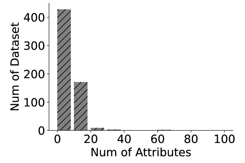
(a) Plot.ly-full

(b) Plot.ly-1k

Figure 1: The distribution of attribute number in the datesets of Plot.ly-full Plot.ly-1k