Rethinking Approximate Gaussian Inference in Classification

Abstract

In classification tasks, softmax functions are ubiquitously used as output activations to produce predictive probabilities. Such outputs only capture aleatoric uncertainty. To capture epistemic uncertainty, approximate Gaussian inference methods have been proposed, which output Gaussian distributions over the logit space. Predictives are then obtained as the expectations of the Gaussian distributions pushed forward through the softmax. However, such softmax Gaussian integrals cannot be solved analytically, and Monte Carlo (MC) approximations can be costly and noisy. We propose a simple change in the learning objective which allows the exact computation of predictives and enjoys improved training dynamics, with no runtime or memory overhead. This framework is compatible with a family of output activation functions that includes the softmax, as well as element-wise normCDF and sigmoid. Moreover, it allows for approximating the Gaussian pushforwards with Dirichlet distributions by analytic moment matching. We evaluate our approach combined with several approximate Gaussian inference methods (Laplace, HET, SNGP) on large- and small-scale datasets (ImageNet, CIFAR-10), demonstrating improved uncertainty quantification capabilities compared to softmax MC sampling. Code is available at github.com/bmucsanyi/probit.

1 Introduction

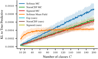
Figure 1: Mean KL divergence between the ‘true’ predictive (approximated with a $10000$ sample MC approximation) and different predictive approximations on a synthetic data set. This synthetic dataset consists of 100 logit means $\bm{\mu}$ and standard deviations $\bm{\sigma}$, whose components are i.i.d. uniformly distributed. For a fair comparison we scale the logit dataset for the different activations to match the activations to first order, so that $\mu_{c}\in[-1,1]$, $\sigma_{c}\in[0,1]$ for sigmoid, $\mu_{c}\in[-1/2-\log 2,1/2-\log 2]$, $\sigma_{c}\in[0,1/2]$ for softmax, $\mu_{c}\in[-\sqrt{\pi/8},\sqrt{\pi/8}]$, $\sigma_{c}\in[0,\pi/8]$ for normCDF. The MC approximations are capped at a fixed computational budget of $10000$ class samples, i.e. $\lceil 10000/C\rceil$ samples. We see that, even without enforcing the constraint Equation 18, our approximations are the only ones that do not become worse with the number of classes. See Appendix C for theoretical analyses of the quality of the different approximations.

Given an input space $\mathcal{X}$, $C$ classes and training data $(x_{n},c_{n})_{n=1}^{N}\subset\mathcal{X}\times\{1,\dots,C\}$, the goal of probabilistic classification is to learn a function $\bm{h}\colon\mathcal{X}\to\Delta^{C-1}$, where

$$\Delta^{C-1}=\{(p_{1},\dots,p_{C})\in[0,1]^{C}:p_{1}+\dots+p_{C}=1\}$$ (1)

is the $(C-1)$-dimensional probability simplex. The model $\bm{h}$ outputs the probability of inputs $x\in\mathcal{X}$ belonging to each class, $h_{c}(x)=p(c\mid x)$. To learn such a map to the simplex, $\bm{h}$ is typically defined as a composition

$$\bm{h}\colon\mathcal{X}\xrightarrow{\quad\bm{f}\quad}\mathbb{R}^{C}\xrightarrow{\operatorname{\mathbf{softmax}}}\Delta^{C-1}$$ (2)

where a function $\bm{f}$, learned from the training data, is mapped through the softmax activation function. In this case, $\mathbb{R}^{C}$ is called the logit space, and, for $x\in\mathcal{X}$, $\bm{f}(x)$ is a logit.

With the usual assumption of i.i.d. data, the likelihood under the model $\bm{h}$ is given by ($\delta$ is the Kronecker delta)

$$p((c_{n})_{n=1}^{N}\mid(x_{n})_{n=1}^{N}) =\prod_{n=1}^{N}p(c_{n}\mid x_{n})$$ (3)

$$=\prod_{n=1}^{N}\prod_{c=1}^{C}h_{c}(x_{n})^{\delta_{c_{n},c}}.$$

This yields a natural loss function for classification problems, the cross-entropy (CE) loss

$$\mathcal{L}((x_{n},c_{n})_{n=1}^{N}) =-\log(p((c_{n})_{n=1}^{N}\mid(x_{n})_{n=1}^{N}))$$ (4)

$$=-\sum_{n=1}^{N}\sum_{c=1}^{C}\delta_{c_{n},c}\log(h_{c}(x_{n})).$$

For typical models $\bm{h}$ trained through such approximate maximum likelihood estimation, an output probability vector $\bm{h}(x)\in\Delta^{C-1}$ should be interpreted as an estimate of $p_{\text{gen}}(\bm{y}\mid x)$, the probability under the generative model. Notably, the output probability does not take into account the uncertainty of the model due to the finite nature of the data. In the uncertainty quantification formalism, such models can only estimate aleatoric uncertainty and disregard epistemic uncertainty (Hüllermeier & Waegeman, 2021).

The probabilistic way to capture epistemic uncertainty is to require the model to output a second-order distribution (as in “a distribution over probability distributions”). That is, for each input $x\in\mathcal{X}$, the model should output a probability measure over the simplex $\mathrm{h}(x)\in\mathcal{P}(\Delta^{C-1})$, as opposed to a point estimate in the simplex $\bm{h}(x)\in\Delta^{C-1}$ (Sensoy et al., 2018; Charpentier et al., 2020).

A number of methods for such distributional uncertainty quantification in classification rely on approximate Gaussian inference in logit space. That is, $\mathrm{h}$ is written as a composition

$$\mathrm{h}\colon\mathcal{X}\xrightarrow{\quad\mathrm{f}\quad}\mathcal{G}(\mathbb{R}^{C})\xrightarrow{\operatorname{\mathbf{softmax}}_{*}}\mathcal{P}(\Delta^{C-1})$$ (5)

where $f$ is learned from the training data, $\mathcal{G}(\mathbb{R}^{C})$ is the set of Gaussian measures on the logit space $\mathbb{R}^{C}$, and $\operatorname{\mathbf{softmax}}_{*}$ pushes forward the Gaussian probability measures through the softmax. For example, Heteroscedastic Classifiers (HET) (Collier et al., 2021) learn the output means and covariances of $\mathrm{f}$ explicitly with a neural network. In linearised Laplace approximations (Daxberger et al., 2021), only the means are learned explicitly with a neural network, while the covariances are obtained post-hoc from that neural network by approximating its parameter posterior distribution with a Gaussian, and then pushing it forward to logit space by linearising the network in the parameters. Last-layer Laplace approximations (Kristiadi et al., 2020) are a variant of linearised Laplace approximations where only the posterior over the last-layer parameters is Gaussian-approximated, requiring no linearisation of the network. Spectral-Normalized Gaussian processes (SNGP) (Liu et al., 2020) are neural networks with last layers that are approximately Gaussian processes, through random feature expansions and Laplace approximations.

To obtain predictive probabilities from a distributional classifier as in Equation 5, we marginalise it out by the measure-theoretic change of variables, using $\mathrm{h}(x)=\operatorname{\mathbf{softmax}}_{*}\mathrm{f}(x)$:

$$\mathbb{E}_{\bm{P}\sim\mathrm{h}(x)}[\bm{P}] =\int_{\Delta^{C-1}}p\;\mathrm{h}(x)(dp)$$ (6)

$$=\int_{\mathbb{R}^{C}}\operatorname{\mathbf{softmax}}(y)\;\mathrm{f}(x)(dy).$$

In addition to predictive probabilities, the distributional framework allows for the acquisition of other quantities of interest, such as variances, entropy, and information-theoretic decompositions of the predictive uncertainty into aleatoric and epistemic parts (Depeweg et al., 2018; Mukhoti et al., 2023; Wimmer et al., 2023). These are usually obtained by Monte Carlo (MC) sampling from the Gaussian measure $\mathrm{f}(x)$. Indeed, while the probability density of $\mathrm{h}(x)=\operatorname{\mathbf{softmax}}_{*}\mathrm{f}(x)$ can be obtained in closed form using a change of variables formula (Atchison & Shen, 1980), this does not seem of practical use. Even predictives cannot be computed analytically. On the other hand, given a variance, the runtime and memory cost required for an MC approximation to achieve an estimator of said variance grows linearly with the number of classes. Crucially, this computational cost is not limited to training time, but also to inference time, when the computational budget may be much more limited. This limits the application of such Gaussian inference methods in classification tasks with large number of classes, such as those common in computer vision and natural language processing.

1.1 Proposed Recipe

We can summarise our framework as a 4-step recipe:

1. Choose an approximate Gaussian inference method: a method that outputs logit covariances.

2. Choose an output activation for which the corresponding Gaussian integral can be solved (Section 2).

3. Train with an objective that enforces a certain normalisation constraint (Section 4).

4. At inference time, use our analytic formulas (see Section 2 for the predictives, Section 3 for other quantities of interest).

2 Gaussian Inference with Analytic Predictives

2.1 Motivation from Softmax Models

A key difficulty in obtaining exact or closed-form approximate predictive probabilities of $\mathrm{h}(x)=\operatorname{\mathbf{softmax}}_{*}\mathrm{f}(x)$ is that pushforwards of Gaussian distributions through the softmax are intractable. The softmax function is the composition $\bm{\operatorname{\mathbf{softmax}}}=\bm{n}\circ\bm{\exp}$, where $\bm{n}$ is the normalisation function given by $\bm{n}(\bm{q}):=\bm{q}/(q_{1}+\dots+q_{C})$ and $\bm{\exp}$ is applied element-wise. Thus, $\mathrm{h}$ can be written as the composition (c.f. Equation 5)

$$\mathrm{h}\colon\mathcal{X}\xrightarrow{\quad\mathrm{f}\quad}\mathcal{G}(\mathbb{R}^{C})\xrightarrow{\bm{\exp}_{*}}\mathcal{P}(\mathbb{R}_{>0}^{C})\xrightarrow{\bm{n}_{*}}\mathcal{P}(\Delta^{C-1}).$$ (7)

Now it is easy to see that (Section A.1)

$$\int_{\mathbb{R}}\exp(y)\;\mathcal{N}(\mu,\sigma^{2})(dy)=\exp\left(\mu+\frac{\sigma^{2}}{2}\right)$$ (8)

and thus

$$\mathbb{E}_{\bm{Q}\sim\bm{\exp}_{*}\mathrm{f}(x)}[\bm{Q}] =\int_{\mathbb{R}^{C}}\bm{\exp}(\bm{y})\;\mathrm{f}(x)(d\bm{y})$$ (9)

$$=\bm{\exp}\left(\bm{\mu}(x)+\frac{\bm{\sigma}^{2}(x)}{2}\right)$$

where $\bm{\mu}(x)$ and $\bm{\sigma}^{2}(x)$ are, respectively, the mean and the diagonal of the covariance of $\mathrm{f}(x)$, and the vector division is element-wise. Note that no approximations are made so far.

We can use this to approximate the predictive of the model in closed form:

$$\mathbb{E}_{\bm{P}\sim\mathrm{h}(x)}[\bm{P}] =\mathbb{E}_{\bm{Q}\sim\bm{\exp}_{*}\mathrm{f}(x)}\left[\frac{\bm{Q}}{\sum_{c=1}^{C}Q_{c}}\right]$$ (10)

$$\approx\frac{\mathbb{E}_{\bm{Q}\sim\bm{\exp}_{*}\mathrm{f}(x)}[\bm{Q}]}{\mathbb{E}_{\bm{Q}\sim\bm{\exp}_{*}\mathrm{f}(x)}\left[\sum_{c=1}^{C}Q_{c}\right]}$$

$$=\frac{\mathbb{E}_{\bm{Q}\sim\bm{\exp}_{*}\mathrm{f}(x)}[\bm{Q}]}{\sum_{c=1}^{C}\mathbb{E}_{Q_{c}\sim\exp_{*}\mathrm{f}_{c}(x)}\left[Q_{c}\right]}$$

$$=\frac{\bm{\exp}\left(\bm{\mu}(x)+\frac{\bm{\sigma}^{2}(x)}{2}\right)}{\sum_{c=1}^{C}\exp\left(\mu_{c}(x)+\frac{\sigma^{2}_{c}(x)}{2}\right)}.$$

2.2 The General Framework

In fact, we can apply the previous argumentation to a general family of output activation functions: suppose we can write the output activation as $\bm{n}\circ\bm{\varphi}$, where $\bm{\varphi}$ is the element-wise application of some activation function $\varphi\colon\mathbb{R}\to\mathbb{R}_{>0}$. So we have (c.f. Equation 7)

$$\mathrm{h}\colon\mathcal{X}\xrightarrow{\quad\mathrm{f}\quad}\mathcal{G}(\mathbb{R}^{C})\xrightarrow{\bm{\varphi}_{*}}\mathcal{P}(\mathbb{R}_{>0}^{C})\xrightarrow{\bm{n}_{*}}\mathcal{P}(\Delta^{C-1}).$$ (11)

If we can solve the one-dimensional integrals (c.f. Equation 8)

$$\int_{\mathbb{R}}\varphi(y)\;\mathcal{N}(\mu,\sigma^{2})(dy)$$ (12)

then we can compute the approximate predictive (c.f. Equation 10)

$$\mathbb{E}_{\bm{P}\sim\mathrm{h}(x)}[\bm{P}]\approx\frac{\mathbb{E}_{\bm{Q}\sim\bm{\varphi}_{*}\mathrm{f}(x)}[\bm{Q}]}{\sum_{c=1}^{C}\mathbb{E}_{Q_{c}\sim\varphi_{*}\mathrm{f}_{c}(x)}\left[Q_{c}\right]}.$$ (13)

For instance, taking $\varphi=\Phi$, the standard Normal cumulative distribution function (normCDF), we have by a classical result (Section A.2),

$$\int_{\mathbb{R}}\Phi(y)\;\mathcal{N}(\mu,\sigma^{2})(dy)=\Phi\left(\frac{\mu}{\sqrt{1+\sigma^{2}}}\right)$$ (14)

and thus

$$\mathbb{E}_{\bm{P}\sim\mathrm{h}(x)}[\bm{P}]\approx\frac{\bm{\Phi}\left(\frac{\bm{\mu}(x)}{\sqrt{1+\bm{\sigma}^{2}(x)}}\right)}{\sum_{c=1}^{C}\Phi\left(\frac{\mu_{c}(x)}{\sqrt{1+\sigma^{2}_{c}(x)}}\right)}.$$ (15)

Taking instead $\varphi=\rho$, the logistic sigmoid, we can approximate Equation 12 with the probit approximation (Section A.3)

$$\int_{\mathbb{R}}\rho(y)\;\mathcal{N}(\mu,\sigma^{2})(dy)\approx\rho\left(\frac{\mu}{\sqrt{1+\frac{\pi}{8}\sigma^{2}}}\right)$$ (16)

yielding in this case

$$\mathbb{E}_{\bm{P}\sim\mathrm{h}(x)}[\bm{P}]\approx\frac{\bm{\rho}\left(\frac{\bm{\mu}(x)}{\sqrt{1+\frac{\pi}{8}\bm{\sigma}^{2}(x)}}\right)}{\sum_{c=1}^{C}\rho\left(\frac{\mu_{c}(x)}{\sqrt{1+\frac{\pi}{8}\sigma^{2}_{c}(x)}}\right)}.$$ (17)

2.3 Making the Approximations Exact

At this point, the approximate Equation 13 may seem ad-hoc. However, note that Equation 13 is exact when $\sum_{c=1}^{C}Q_{c}$ is a constant random variable, as can be seen from the derivation in Equation 10. Thus, we would like to enforce a constraint in the model of the form

$$\sum_{c=1}^{C}Q_{c} =s(x) \text{where }\bm{Q}\sim\bm{\varphi}_{*}\mathrm{f}(x)$$ (18)

where $s\colon\mathcal{X}\to\mathbb{R}$ is a deterministic function. In other words, the law of $\sum_{c=1}^{C}Q_{c}$ is a Dirac measure for all $x$.

In neural networks, constraints can be learned through appropriate choices of learning objectives during training, ensuring that they are satisfied within the training data distribution. In Section 4, we describe how this can be achieved depending on $\bm{\varphi}$ and the method that is used to obtain the mapping to Gaussian distributions $\mathrm{f}$.

Given the constraint of Equation 18 is satisfied, Equations 10 and 15 ($\varphi=\exp\text{ or }\Phi$) both become exact. For Equation 17 ($\varphi=\rho$), the only error incurred is the one from the probit approximation (Equation 16) per each class. In the synthetic experiment (Figure 1), we see that this induces no significant effect on the quality of the predictive. We justify this observation with the following result:

Theorem 2.1.

Let $\varphi=\rho$. Suppose that the logit means and variances $(\mu_{c},\sigma^{2}_{c})$ lie in some compact set $\mathcal{K}\subset\mathbb{R}\times\mathbb{R}_{>0}$ for each class $c$. Then, assuming the constraint Equation 18 is perfectly satisfied, the KL divergence between the true and approximate predictive Equation 17 is bounded by some constant $M(\mathcal{K})$ only depending on $\mathcal{K}$, not on $C$.

Section C.2 provides a more precise statement, a formula for $M(\mathcal{K})$, and a proof. Importantly, this result states that the approximation error does not increase with the number of classes.

Finally, observe that, when enforcing Equation 18, we obtain exact predictives with Equation 13, which only uses the diagonal of $\mathrm{f}(x)$’s covariance. Enforcing this constraint thus allows one to ignore non-diagonal terms in the logit covariances. In Section 5, we discuss how this can be leveraged for computational gains.

3 Distributional Approximations of the Gaussian Pushforwards

3.1 Dirichlet Matching

While in many applications, predictive probabilities are all that is needed from a model, we set out to build a model that outputs a tractable probability distribution over the simplex $\mathrm{h}(x)\in\mathcal{P}(\Delta^{C-1})$. As previously discussed, such a distribution allows, for instance, closed-form decompositions of aleatoric and epistemic uncertainties.

The formulation of Equation 11 does not yet allow this. However, we will now see that we can obtain good Dirichlet approximations by constructing a tractable approximation of Equation 11 of the form

$$\mathrm{h}\colon\mathcal{X}\xrightarrow{\quad\mathrm{f}\quad}\mathcal{G}(\mathbb{R}^{C})\xrightarrow{\quad\mathrm{a}\quad}\mathcal{D}(\Delta^{C-1}),$$ (19)

where $\mathcal{D}(\Delta^{C-1})$ is the space of Dirichlet distributions on $\Delta^{C-1}$. The family of Dirichlets presents an ideal choice of distributions over the simplex as, for such distributions, all quantities of interest can be computed analytically (c.f. Appendix G). The map $\mathrm{a}$ is constructed by moment matching: we match the first two moments of the Dirichlet distribution to the moments of the Gaussian pushforward $\bm{\varphi}_{*}\mathrm{f}(x)$.

Conveniently, just as the first moments described in Section 2, we can obtain second moments for $\exp$

$$\int_{\mathbb{R}}\exp(y)^{2}\;\mathcal{N}(\mu,\sigma^{2})(dy)=\exp(2\mu+2\sigma^{2})$$ (20)

and for $\Phi$ (Owen (1980, Eq. 20,010.4))

$$\int_{\mathbb{R}}\Phi(y)^{2}\;\mathcal{N}(\mu,\sigma^{2})(dy)$$ (21)

$$\quad=\Phi\left(\frac{\mu}{\sqrt{1+\sigma^{2}}}\right)-2T\left(\frac{\mu}{\sqrt{1+\sigma^{2}}},\frac{1}{\sqrt{1+2\sigma^{2}}}\right),$$

where $T$ is Owen’s T function. For $\rho$, we have the following approximation (Daunizeau (2017, Equation 23))

$$\int_{\mathbb{R}}\rho(y)^{2}\;\mathcal{N}(\mu,\sigma^{2})(dy)\approx\rho\left(\frac{\mu}{\sqrt{1+\frac{\pi}{8}\sigma^{2}}}\right)$$ (22)

$$-\frac{\rho\left(\frac{\mu}{\sqrt{1+\frac{\pi}{8}\sigma^{2}}}\right)\left(1-\rho\left(\frac{\mu}{\sqrt{1+\frac{\pi}{8}\sigma^{2}}}\right)\right)}{\sqrt{1+\frac{\pi}{8}\sigma^{2}}}.$$

This enables us to compute the second moment of the pushforward distribution via

$$\mathbb{E}_{\bm{P}\sim\bm{n}_{*}\bm{\varphi}_{*}\mathrm{f}(x)}[\bm{P}^{2}] =\mathbb{E}_{\bm{Q}\sim\bm{\varphi}_{*}\mathrm{f}(x)}\left[\frac{\bm{Q}^{2}}{\left(\sum_{c=1}^{C}Q_{c}\right)^{2}}\right]$$ (23)

$$\approx\frac{\mathbb{E}_{\bm{Q}\sim\bm{\varphi}_{*}\mathrm{f}(x)}[\bm{Q}^{2}]}{\mathbb{E}_{Q_{c}\sim\varphi_{*}\mathrm{f}_{c}(x)}\left[\sum_{c=1}^{C}Q_{c}\right]^{2}}.$$

As in Equation 13, the approximation in Equation 23 is exact when $\sum_{c=1}^{C}Q_{c}$ is a constant random variable, as under the constraint of Equation 18.

If we were to directly attempt to infer the parameters of the Dirichlet $\mathrm{h}(x)$ from Equations 13 and 23, we would obtain an overparametrised system of equations with $2C$ equations and $C$ unknowns. Thus, we instead use a classical Dirichlet method of moments (Minka, 2000, Eqs. 19 & 23), which reduces these equations, as we will now describe.

The sum of the Dirichlet parameters $\sum_{c=1}^{C}\gamma_{c}$ may be estimated by

$$\frac{\mathbb{E}[P_{c}]-\mathbb{E}[P^{2}_{c}]}{\mathbb{E}[P^{2}_{c}]-\mathbb{E}[P_{c}]^{2}}$$ (24)

for any $1\leq c\leq C$. So, a natural estimate of $\sum_{c=1}^{C}\gamma_{c}$ that uses all $P_{c}$ is the geometric mean of Equation 24. Since the mean of the Dirichlet is $\bm{\gamma}/\sum_{c=1}^{C}\gamma_{c}$, we obtain using Equation 24 an expression for the Dirichlet parameters

$$\left(\prod_{c=1}^{C}\frac{\mathbb{E}[P_{c}]-\mathbb{E}[P^{2}_{c}]}{\mathbb{E}[P^{2}_{c}]-\mathbb{E}[P_{c}]^{2}}\right)^{1/C}\mathbb{E}[\bm{P}].$$ (25)

Hence, using Equations 13 and 23, we obtain the computationally feasible Dirichlet parameters

$$\bm{\gamma}:=\left(\prod_{c=1}^{C}\frac{\mathbb{E}[Q_{c}]\cdot S-\mathbb{E}[Q^{2}_{c}]}{\mathbb{E}[Q^{2}_{c}]-\mathbb{E}[Q_{c}]^{2}}\right)^{1/C}\left(\frac{\mathbb{E}[\bm{Q}]}{\sum_{c=1}^{C}\mathbb{E}[Q_{c}]}\right)$$ (26)

for $\mathrm{h}(x)$, where $S=\max(\sum_{c=1}^{C}\mathbb{E}[Q_{c}],1)$. Taking the maximum with $1$ in the expression for $S$ is an additional approximation to ensure $\bm{\gamma}\geq\bm{0}$, and is justified when taking $s(x)=1$ for all $x$ in Equation 18. Note that performing such moment matching to obtain the Dirichlet parameters in Equation 26, the mean of this Dirichlet matches precisely the approximate predictive Equation 13. That is, the approximate predictive of the exact distributional model (Equation 11) matches the exact predictive of the approximate distributional model (Equation 19).

3.2 Intermediate Beta Matching

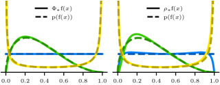
Figure 2: Approximating Gaussian pushforwards $\Phi_{*}\mathrm{f}(x)$ and $\rho_{*}\mathrm{f}(x)$ through normCDF and sigmoid respectively by Beta distributions $\mathrm{p}(\mathrm{f}(x))$ with moment matching. With normCDF, we can match exact moments, whereas with sigmoid, we match approximate moments. Moreover, when $\mathrm{f}(x)$ is the standard Normal $\mathcal{N}(0,1)$ (on the left in blue), the approximation for the pushforward through normCDF is exact (Section D.1).

When $\varphi=\Phi\text{ or }\rho$, noting that their range is $(0,1)$, we can decompose the approximate distributional model (Equation 19) further:

$$\mathrm{h}\colon\mathcal{X}\xrightarrow{\quad\mathrm{f}\quad}\mathcal{G}(\mathbb{R}^{C})\xrightarrow{\mathrm{p}}\mathcal{B}((0,1))^{C}\xrightarrow{\mathrm{n}}\mathcal{D}(\Delta^{C-1}),$$ (27)

where $\mathcal{B}((0,1))$ is the space of Beta distributions on $(0,1)$. Like the output Dirichlets, we obtain the intermediate Beta distributions by moment matching (Appendix D). Figure 2 indicates that such Beta approximations tend to be of high quality. In Section D.1, we give an information-geometric motivation for this, which shows that the choice of activation $\Phi$ is ideal for approximating the Gaussian pushforwards with Beta distributions.

The quality of such Beta approximations is encouraging for that of the output Dirichlet approximations: observe that taking $s(x)=1$ for all $x$ in Equation 18, $\bm{n}$ becomes the identity (as it normalises by 1), and thus all $\mathrm{n}$ does is combining the $C$ Beta approximations into one Dirichlet.

4 Learning the Constraint

As discussed in Sections 2.3 and 3, the quality of our approximations relies on the enforcement of the constraint $\sum_{c=1}^{C}Q_{c}=s(x)$ for some deterministic function $s\colon\mathcal{X}\to\mathbb{R}$ (Equation 18). In this work, we simply choose $s(x)=1$ for all $x$. We thus make use of the degree of freedom in the logits to obtain exact predictives in Equation 13. In Appendix E, we make the connection with the energy-based model view of classifiers (Grathwohl et al., 2019), which instead makes use of this degree of freedom to turn discriminative models into generative models. Future work could combine both frameworks by learning $s(x)\propto p_{\operatorname{gen}}(x)$.

4.1 Explicit Constraint

Up to this point, we have treated the model $\mathrm{f}$ as a black box. However, to discuss how to impose Equation 18, we need to think about the specifics of how such models are trained and how Gaussian distributions are then obtained.

In linearised Laplace approximations and SNGP, a neural network $\bm{f}\colon\mathcal{X}\to\mathbb{R}^{C}$ is trained for the mean of $\mathrm{f}$, while the covariance is obtained post-hoc. Therefore, to enforce Equation 18 on the training data distribution, we can train for $\sum_{c=1}^{C}\varphi(f_{c}(x_{n}))=1$ for all $1\leq n\leq N$.

This can be achieved, for example, by adding an appropriate regulariser to the loss. Namely,

$$\mathcal{L}((x_{n},c_{n})_{n=1}^{N})$$ (28)

$$\quad=\tilde{\mathcal{L}}((x_{n},c_{n})_{n=1}^{N})+\lambda\sum_{n=1}^{N}\left(\sum_{c=1}^{C}\varphi(f_{c}(x_{n}))-1\right)^{2}$$

for some tuned regularisation constant $\lambda$, where $\tilde{\mathcal{L}}$ is the original unregularised loss.

In contrast to the previously mentioned methods, HET directly trains not only for the mean $\bm{f}$ but also for the covariance matrix $\bm{\Sigma}$ of $\mathrm{f}$ through the predictives. Thus, in this case, we can regularise with the means of the Gaussian pushforwards through $\varphi$:

$$\mathcal{L}((x_{n},c_{n})_{n=1}^{N}) =\tilde{\mathcal{L}}((x_{n},c_{n})_{n=1}^{N})$$ (29)

$$+\lambda\sum_{n=1}^{N}\left(\sum_{c=1}^{C}\mathbb{E}_{Q_{c}\sim\varphi_{*}\mathrm{f}_{c}(x)}[Q_{c}]-1\right)^{2}.$$

In Section 6, we will see that training with such a learning objective does not always outperform vanilla CE training. For $\varphi=\exp$, for instance, we observe that the regulariser can take on extreme values, dominating the data term, slowing down training.

We shall now see that, when $\varphi$ has range $(0,1)$, we can enforce the constraint with the learning objective in a more natural, implicit way.

4.2 Implicit Constraint

In the case of $\varphi=\Phi\text{ or }\rho$, $\sum_{c=1}^{C}\varphi(f_{c}(x_{n}))=1$ can be achieved more advantageously: since the range of $\Phi$ and $\rho$ is $(0,1)$, under the condition $\sum_{c=1}^{C}\varphi(f_{c}(x_{n}))=1$, we can view $\varphi(f_{c}(x_{n}))$ as estimates of $p(c\mid x_{n})$. This motivates the use of class-wise cross-entropy losses (class-wise CE).

For linearised Laplace approximations and SNGP, which solely train a mean $\bm{f}$, the class-wise CE is given by

$$\mathcal{L}((x_{n},c_{n})_{n=1}^{N}) =-\sum_{n=1}^{N}\sum_{c=1}^{C}\big{(}\delta_{c_{n},c}\log(\varphi(f_{c}(x)))$$ (30)

$$\quad+(1-\delta_{c_{n},c})\log(1-\varphi(f_{c}(x))\big{)}.$$

The labels being one-hot vectors and the binary cross-entropy loss being a (negative) strictly proper scoring rule (c.f. Appendix I) together ensure that Equation 30 enforces the soft constraint $\sum_{c=1}^{C}\varphi\circ\mu_{c}=1$ on the training data, and hence in the training data distribution (Figure 3).

We note that the loss Equation 30 is only used for training and not for inference or evaluation. Indeed, methods such as Laplace approximations and SNGP – which rely on negative log-likelihood losses to obtain an approximate Gaussian distribution – can then use the actual log-likelihood loss of the model, that is, the cross-entropy loss of $\bm{n}\circ\bm{\varphi}\circ\bm{f}$.

Similarly, for HET, we use the class-wise CE with the pushforward means

$$\mathcal{L}((x_{n},c_{n})_{n=1}^{N}) =-\sum_{n=1}^{N}\sum_{c=1}^{C}\big{(}\delta_{c_{n},c}\log(\mathbb{E}_{Q_{c}\sim\varphi_{*}\mathrm{f}_{c}(x)}[Q_{c}])$$ (31)

$$+(1-\delta_{c_{n},c})\log(1-\mathbb{E}_{Q_{c}\sim\varphi_{*}\mathrm{f}_{c}(x)}[Q_{c}])\big{)}.$$

Enforcing the constraint in this implicit way is powerful since, in contrast to the regularised CE objective (Equation 28), the class-wise CE (Equation 30) fully aligns with the task. In Section 6 we shall see that training on class-wise CE generally outperforms softmax CE training.

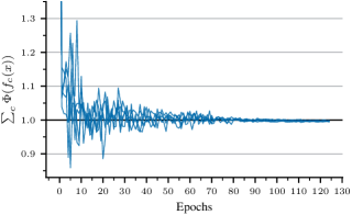
Figure 3: Evolution of the constraint on validation data for normCDF models trained on ImageNet.

5 Computational Gains

The runtime cost of the MC predictive approximation is $\mathcal{O}(S\cdot C+C^{3})$, and the memory cost is $\mathcal{O}(S\cdot C+C^{2})$, where $S$ is the number of samples. The $C^{2}$ term in memory comes from the logit covariance matrix; the $C^{3}$ term in runtime comes from the need to Cholesky-decompose such covariance matrix before sampling. For example, on a ResNet-50, sampling one thousand logit vectors from the logit-space Gaussian means an approximately 7% overhead on the forward pass. In embedded systems with much smaller models, this overhead is even larger. In contrast, the runtime and memory cost of calculating a predictive through our framework is $\mathcal{O}(C)$, which is negligible in comparison.

Indeed, as noted at the end of Section 2.3, the constraint (Equation 18) ensures that only the mean and the diagonal of the logit covariance are needed in order to calculate the predictive exactly. That is, the logit quantities required to compute a predictive scale as $\mathcal{O}(C)$ instead of $\mathcal{O}(C^{2})$. This provides further opportunities for computational savings in the methods used to obtain the Gaussian distributions.

In HET, for example, the logit covariance is trained with both a diagonal term and a low-rank term. Our framework thus allows one to drop the low-rank term without losing any expressivity in the model.

In SNGP, the off-diagonal terms of the logit covariance are ignored (Liu et al., 2023, p. 47). For unconstrained models, this incurs an approximation error as the inter-class covariance structure can encode vital information for inference. When Equation 18 is satisfied, however, we are guaranteed not to lose expressivity for the predictive computation by discarding the off-diagonal covariance terms, theoretically backing the approximation in SNGP.

6 Experiments

We now investigate our two research questions:

• Do we have to sacrifice performance for sample-free predictives?

• What are the effects of changing the learning objective?

To answer the first question, we consider fixed (method, activation) pairs and verify that our methods perform on par with the Monte Carlo sampled predictives in Section 6.1.

We train four classes of models: Softmax ($\varphi=\exp$, trained with vanilla CE), Exp ($\varphi=\exp$, trained with the explicit constraint (Section 4.1)), NormCDF ($\varphi=\Phi$, trained with the implicit constraint, (Section 4.2)) and Sigmoid ($\varphi=\rho$, trained with the implicit constraint, (Section 4.2)).

We consider Heteroscedastic Classifiers (HET) (Collier et al., 2021), Spectral-Normalized Gaussian Processes (SNGP) (Liu et al., 2020), and last-layer Laplace approximation methods (Daxberger et al., 2021) as backbones. The resulting 18 (method, activation, predictive) triplets are evaluated on ImageNet-1k (Deng et al., 2009) and CIFAR-10 (Krizhevsky & Hinton, 2009) on five metrics aligning with practical needs from uncertainty estimates (Mucsányi et al., 2023). Further, we test the Out-of-Distribution (OOD) detection capabilities of the models on balanced mixtures of In-Distribution (ID) and OOD samples. For ImageNet, we treat ImageNet-C (Hendrycks & Dietterich, 2019) samples with 15 corruption types and 5 severity levels as OOD samples. For CIFAR-10, we use the CIFAR-10C corruptions.

For the second question, we evaluate our analytic predictives and moment-matched Dirichlets against softmax models with approximate inference tools – Laplace Bridge (Hobbhahn et al., 2022) and Mean Field (Lu et al., 2021) approximations, as well as MC sampling, in Section 6.2.

To provide a fair comparison, we reimplement each method as simple-to-use wrappers around deterministic backbones. For ImageNet evaluation, we use a ResNet-50 backbone pretrained with the softmax activation function, and train each (method, activation) pair for 50 ImageNet-1k epochs following Mucsányi et al. (2024). On CIFAR-10, we train ResNet-28 models from scratch for 100 epochs. We search for ideal hyperparameters and checkpoints with a ten-step Bayesian Optimization scheme (Shahriari et al., 2015) in Weights & Biases (Biewald, 2020).

The main paper focuses on ImageNet results to highlight the scalability of our framework and only shows proper scoring results for CIFAR-10. For a complete overview of CIFAR-10 results, refer to Appendix K.

In all plots of the main paper and the Appendix, the error bars are calculated over five independent runs with different seeds and show the minimum and maximum performance.

Table 1: Comparison of ECE results for different predictives using a fixed Laplace backbone.

Method	Mean	Std
Sigmoid Laplace
Analytic	0.0101	0.0006
MC 1000	0.0153	0.0011
MC 100	0.0153	0.0012
MC 10	0.0165	0.0014
NormCDF Laplace
MC 10	0.0112	0.0005
Analytic	0.0114	0.0007
MC 100	0.0115	0.0006
MC 1000	0.0118	0.0007

6.1 Quality of Sample-Free Predictives

In this section, we investigate our first research question: whether there is a price to pay for sample-free predictives and second-order distributions. To this end, we take the two best-performing methods on the Expected Calibration Error (ECE) metric (Naeini et al., 2015), NormCDF and Sigmoid Laplace (c.f. Figure 6) and evaluate their per-predictive performance. As Table 1 shows, the analytic predictive is always on par with the (unbiased) MC estimates on ImageNet while being cheaper. This empirical observation supports our theoretical claim that when the constraint is satisfied, the analytic predictives are exact. Refer to Appendix L for an evaluation of the moment-matched Dirichlet distributions.

6.2 Effects of Changing the Learning Objective

The previous section shows that for an already trained model that satisfies the constraint (Equation 18), our analytic predictives always perform on par with MC sampling while being more efficient. However, our proposed objectives (Sections 4.1 and 4.2) change the training dynamics of models. Therefore, in this section, we showcase the performance of methods equipped with our analytic (i.e., sample-free) predictives and learning objectives against softmax models. For the latter, we use the best-performing predictive and estimator (excluding ours). See Appendices F and G for an overview of predictives and estimators. We employ our methods with the analytic predictives and second-order Dirichlet distributions to demonstrate their competitive nature while being more efficient than MC sampling.

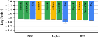
Figure 4: ImageNet log probability proper scoring results. Analytic predictives with implicit ( ) constraints are either on par with or outperform Softmax ( ) on all methods.

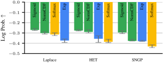
Figure 5: CIFAR-10 log probability proper scoring results. Analytic predictives with implicit ( ) constraints consistently outperform Softmax ( ) on all methods.

We first evaluate how calibrated the models are using the log probability scoring rule (Gneiting & Raftery, 2007) and the Expected Calibration Error (ECE) metric (Naeini et al., 2015). Figure 5 shows that on CIFAR-10, the score of our analytic predictives with implicit constraints (Sigmoid, NormCDF) are consistently better than the corresponding Softmax results for all methods. On the large-scale ImageNet dataset, Sigmoid and NormCDF either outperform or are on par with Softmax.

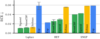
Figure 6: ImageNet ECE results. Analytic predictives with implicit constraints ( ) outperform Softmax ( ) across all methods. Explicit constraints ( ) work best on HET but do not benefit the other two methods. Note the restricted $y$-limits for readability.

The ECE requires the models’ confidence to match their accuracy. Figure 6 shows that on ImageNet, our analytic predictives with implicit constraints (Sigmoid, NormCDF) have a clear advantage over Softmax across all methods. Explicit constraints benefit SNGP and HET but not the post-hoc Laplace method.

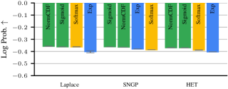
Figure 7: ImageNet log probability proper scoring results for the binary correctness prediction task. Analytic predictives with implicit ( ) constraints consistently outperform Softmax ( ).

Next, we turn to the correctness prediction task: whether the models can predict the correctness of their own predictions. We consider correctness estimators $\tilde{c}(x)\in[0,1]$ for inputs $x\in\mathcal{X}$ derived from the predictives. Framed as a binary prediction task, the goal of these estimators is to predict the probability of the predicted class’ correctness. We then measure the binary log probability score of $\tilde{c}(x)$. Figure 7 shows that our analytic predictives with implicit constraints outperform all Softmax predictives across all methods.

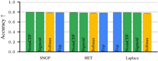
Figure 8: Analytic predictives do not sacrifice accuracy. ImageNet validation accuracies. Analytic predictives with implicit ( ) or explicit ( ) constraints either outperform or are on par with Softmax ( ) across all methods.

Analytic predictives do not sacrifice accuracy.

Figure 8 evidences this claim on ImageNet: our analytic predictives either outperform or are on par with Softmax predictives. The most accurate methods are NormCDF and Sigmoid SNGP. These results are in line with the findings of Wightman et al. (2021), who also recommend training with a per-class binary cross-entropy loss using the sigmoid activation function.

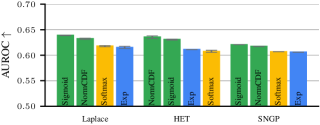
Figure 9: ImageNet OOD detection AUROC results for severity level one. Across all methods, the best-performing predictive is analytic with an implicit constraint ( ).

Finally, we consider another binary prediction task, where a general uncertainty estimator $u(x)\in\mathbb{R}$ (derived from predictives or second-order Dirichlet distributions) is tasked to separate ID and OOD samples from a balanced mixture. As the uncertainty estimator can take on any real value, we measure the Area Under the Receiver Operating Characteristic curve (AUROC), which quantifies the separability of ID and OOD samples w.r.t. the uncertainty estimator. As OOD inputs, we consider corrupted ImageNet-C (Hendrycks & Dietterich, 2019) samples. Figure 9 shows that our analytic predictives with implicit constraints (Sigmoid, NormCDF) outperform Softmax across all methods, even though separating ID and OOD samples does not require a fine-grained representation of uncertainty, unlike the ECE or proper scoring rules. Importantly, these analytic predictives and second-order Dirichlet distributions are considerably cheaper to calculate than Softmax MC predictions (see Section 5). See Appendix M for the other severity levels.

7 Conclusion and Limitations

We developed a framework that allows to obtain predictives and other quantities of interest from logit space Gaussian distributions analytically. Our experimental results suggest the ubiquitous softmax activation should be replaced by normCDF or sigmoid.

We proposed to approximate the Gaussian pushforwards by Dirichlet distributions which cannot encode correlations between classes. Leveraging a more expressive yet tractable family of distributions on the simplex that can achieve this presents an interesting area of future research.

Impact Statement

This paper presents work whose goal is to advance the field of Machine Learning. There are many potential societal consequences of our work, none of which we feel must be specifically highlighted here.

Appendix A Gaussian Integral Derivations

In this appendix, we derive the closed-form formula for the mean of Gaussian pushforwards through exp (Equation 8) and normCDF (Equation 14), as well as the approximations for pushforwards through sigmoid (Equation 16) and softmax.

A.1 Gaussian Exp Integral

By absorbing the exponential into the Gaussian probability density function, we get

$$\int_{\mathbb{R}}\exp(y)\;\mathcal{N}(\mu,\sigma^{2})(dy) =\int_{\mathbb{R}}\exp(y)\exp\left(-\frac{(y-\mu)^{2}}{2\sigma^{2}}\right)\;dy$$ (32)

$$=\int_{\mathbb{R}}\exp\left(\mu+\frac{\sigma^{2}}{2}\right)\exp\left(-\frac{1}{2\sigma^{2}}(y-\mu-\sigma^{2})^{2}\right)\;dy$$

$$=\int_{\mathbb{R}}\exp\left(\mu+\frac{\sigma^{2}}{2}\right)\;\mathcal{N}(\mu+\sigma^{2},\sigma^{2})(dy)$$

$$=\exp\left(\mu+\frac{\sigma^{2}}{2}\right).$$

A.2 Gaussian NormCDF Integral

Here, we derive the classical normCDF Gaussian integration formula (Owen, 1980, Eq. 10,010.8).

For $\lambda>0$, $Z\sim\mathcal{N}(0,1)$ and $Y\sim\mathcal{N}(\mu,\sigma^{2})$ with $Y$ and $Z$ independent,

$$\int_{\mathbb{R}}\Phi(\lambda y)\;\mathcal{N}(\mu,\sigma^{2})(dy) =\int_{\mathbb{R}}p(Z\leq y/\lambda)\;\mathcal{N}(\mu,\sigma^{2})(dy)$$ (33)

$$=p\left(Z\leq\frac{Y}{\lambda}\right)$$

$$=p\left(\frac{Z/\lambda-Y+\mu}{\sqrt{\lambda^{-2}+\sigma^{2}}}\leq\frac{\mu}{\sqrt{\lambda^{-2}+\sigma^{2}}}\right)$$

$$=\Phi\left(\frac{\mu}{\sqrt{\lambda^{-2}+\sigma^{2}}}\right)$$

where we used $\frac{Z/\lambda-X+\mu}{\sqrt{\lambda^{-2}+\sigma^{2}}}\sim\mathcal{N}(0,1)$ for the last equality. Taking $\lambda=1$, this gives the formula for the exact predictive with normCDF.

A.3 Probit Approximation for Gaussian Sigmoid Integral

Taylor expanding $\rho$ to first order about $0$,

$$\rho(y) =\frac{1}{2}+\frac{1}{4}y+o(y)$$ (34)

$$\Phi(y) =\frac{1}{2}+\frac{1}{\sqrt{2\pi}}y+o(y).$$

Hence matching $\rho$ and $\Phi$ to first order we get the approximation $\rho(y)\approx\Phi\left(\sqrt{\frac{\pi}{8}}y\right)$. So using Equation 33 we derive the probit approximation (Spiegelhalter & Lauritzen, 1990; MacKay, 1992)

$$\int_{\mathbb{R}}\rho(y)\;\mathcal{N}(\mu,\sigma^{2})(dy)\stackrel{{\scriptstyle(1)}}{{\approx}}\int_{\mathbb{R}}\Phi\left(\sqrt{\frac{\pi}{8}}y\right)\;\mathcal{N}(\mu,\sigma^{2})(dy)=\Phi\left(\frac{\mu}{\sqrt{\frac{8}{\pi}+\sigma^{2}}}\right)\stackrel{{\scriptstyle(2)}}{{\approx}}\rho\left(\frac{\mu}{\sqrt{1+\frac{\pi}{8}\sigma^{2}}}\right).$$ (35)

Note that the approximation (2) is not strictly needed, as $\Phi$ is computationally tractable. However, adding (2) empirically improves the quality of the overall approximation. This may be due to the fact the thicker tails of $\rho$ in the integrand of the left-hand side are better captured by $\rho$ than $\Phi$ on the right-hand side.

A.4 Mean Field Approximation for Gaussian Softmax Integral

For $\bm{\mu}\in\mathbb{R}^{C}$, $\bm{\sigma}^{2}\in\mathbb{R}^{C}_{>0}$ and $\bm{\Sigma}=\operatorname{\mathbf{diag}}(\bm{\sigma}^{2})$, the mean field approximation to the Gaussian softmax integral (Lu et al., 2021) is obtained as follows

$$\mathbb{E}_{\bm{Y}\sim\mathcal{N}(\bm{\mu},\bm{\Sigma})}[\operatorname{softmax}_{c}\bm{Y}] =\mathbb{E}\left[\left(2-C+\sum_{c^{\prime}\neq c}\rho(Y_{c}-Y_{c^{\prime}})^{-1}\right)^{-1}\right]$$ (36)

$$\stackrel{{\scriptstyle(1)}}{{\approx}}\left(2-C+\sum_{c^{\prime}\neq c}\mathbb{E}[\rho(Y_{c}-Y_{c^{\prime}})]^{-1}\right)^{-1}$$

$$\stackrel{{\scriptstyle(2)}}{{\approx}}\left(2-C+\sum_{c^{\prime}\neq c}\mathbb{E}[\rho(Y_{c}-\mu_{c^{\prime}})]^{-1}\right)^{-1}$$

$$\stackrel{{\scriptstyle(3)}}{{\approx}}\left(2-C+\sum_{c^{\prime}\neq c}\rho\left(\frac{\mu_{c}-\mu_{c^{\prime}}}{\sqrt{1+\frac{\pi}{8}\sigma_{c}^{2}}}\right)^{-1}\right)^{-1}$$

$$=\operatorname{softmax}_{c}\left(\frac{\bm{\mu}}{\sqrt{1+\frac{\pi}{8}\bm{\sigma}^{2}}}\right)$$

i.e.,

$$\mathbb{E}_{\bm{Y}\sim\mathcal{N}(\bm{\mu},\bm{\Sigma})}[\operatorname{\mathbf{softmax}}\bm{Y}]\approx\operatorname{\mathbf{softmax}}\left(\frac{\bm{\mu}}{\sqrt{1+\frac{\pi}{8}\bm{\sigma}^{2}}}\right).$$ (37)

(1) is the mean field approximation, and (3) uses the probit approximation Equation 35. (Lu et al., 2021) provides two other variants of this approximation with other choices of approximation (2).

Appendix B Comparison with the Multinomial Probit Model

In this appendix, we show that a model whose output activation is a composition of an element-wise normCDF activation $\bm{\Phi}$ and a normalisation $\bm{n}$ is distinct from the classical multinomial probit model (Daganzo, 1979).

Given a logit $\bm{y}\in\mathbb{R}^{C}$, the multinomial probit model sets

$$Z(\bm{y})=\operatorname*{arg\,max}_{1\leq c\leq C}Y_{c}$$ (38)

where $Y_{c}=y_{c}+\epsilon_{c}$ and the $\epsilon_{c}$ are i.i.d. standard Normal. So

$$p(c\mid y)=p(y_{c}+\epsilon_{c}>y_{c^{\prime}}+\epsilon_{c^{\prime}}\;\forall\>c^{\prime}\neq c)$$ (39)

which is generally not analytically tractable. On the other hand, a model that uses normCDF and normalisation as output activation yields

$$p(c\mid y)=\frac{p(y_{c}+\epsilon_{c}>0)}{\sum_{c^{\prime}=1}^{C}p(y_{c^{\prime}}+\epsilon_{c^{\prime}}>0)}=\frac{\Phi(y_{c})}{\sum_{c^{\prime}=1}^{C}\Phi(y_{c}^{\prime})}.$$ (40)

In the case $C=2$, the multinomial probit model Equation 39 outputs closed form probabilities. This allows us to construct an explicit counterexample to the equivalence of the two models Equation 39 and Equation 40:

$$p(y_{1}+\epsilon_{1}>y_{2}+\epsilon_{2}) =p\left(\frac{y_{1}-y_{2}}{2}+\frac{\epsilon_{1}-\epsilon_{2}}{2}>0\right)=\Phi\left(\frac{y_{1}-y_{2}}{2}\right)\neq\frac{\Phi(y_{1})}{\Phi(y_{1})+\Phi(y_{2})}.$$ (41)

Appendix C Analysis of the Predictive Approximations’ Quality

In this appendix, we provide theoretical analyses of the quality of various predictive approximations. This complements the empirical analyses taken, for instance, in the synthetic experiment (Figure 1) or in (Daunizeau, 2017).

Due to its information-theoretic interpretation, a natural metric to equip the probability simplex $\Delta^{C-1}$ with is the KL divergence

$$\operatorname{D_{KL}}(\bm{p},\bm{q})=\sum_{c=1}^{C}p_{c}(\log p_{c}-\log q_{c})$$ (42)

which is well defined if $\bm{p}$, $\bm{q}$ lie in the interior of the simplex ($p_{i},q_{i}\neq 0,1$ for all $i$). So, for a predictive approximation, $\bm{\hat{p}}$, we would like to analyse $\operatorname{D_{KL}}(\bm{p},\bm{\hat{p}})$, where $\bm{p}:=\mathbb{E}_{\bm{P}\sim\bm{a}_{*}\mathcal{N}(\bm{\mu},\bm{\Sigma})}[\bm{P}]$ is the true predictive, $\bm{\mu}$ and $\bm{\Sigma}$ are some logit space mean and covariance and $\bm{a}$ is an output activation (e.g. $\bm{a}=\bm{n}\circ\bm{\varphi}$).

C.1 Analysis of Monte Carlo Approximations

An $N$ sample Monte Carlo estimate is defined as

$$\bm{\hat{P}}^{S}:=\frac{1}{S}\sum_{s=1}^{S}\bm{\hat{P}}^{(s)}$$ (43)

where the $\bm{\hat{P}}^{(s)}$ are i.i.d. $\bm{a}_{*}\mathcal{N}(\bm{\mu},\bm{\Sigma})$. The computational cost of MC integration is $\mathcal{O}(S\cdot C)$. This becomes prohibitive for large $S$ and $C$. Thus, for a fair assessment of the quality of such an estimate in terms of the number of classes, one should consider MC estimates $\bm{\hat{P}}^{\lceil S/C\rceil}$.

We now give an informal theoretical argument for the linear growth of the KL divergence between $\bm{p}$ and $\bm{\hat{P}}^{\lceil S/C\rceil}$ in terms of $C$, under the distributional conditions of the synthetic experiment (Figure 1).

Taylor expanding Equation 42 about $\bm{p}$ to second order we obtain

$$\operatorname{D_{KL}}(\bm{p},\bm{q}) =\sum_{c=1}^{C}p_{c}(\log p_{c}-\log q_{c})$$ (44)

$$=\sum_{c=1}^{C}p_{c}\sum_{k=1}^{\infty}\frac{(p_{c}-q_{c})^{k}}{kp_{c}^{k}}$$

$$=\underbrace{\sum_{c=1}^{C}p_{c}}_{=1}-\underbrace{\sum_{c=1}^{C}q_{c}}_{=1}+\sum_{c=1}^{C}\sum_{k=2}^{\infty}\frac{(p_{c}-q_{c})^{k}}{kp_{c}^{k-1}}$$

$$\stackrel{{\scriptstyle(1)}}{{\approx}}\sum_{c=1}^{C}\frac{(p_{c}-q_{c})^{2}}{2p_{c}}$$

$$\stackrel{{\scriptstyle(2)}}{{\approx}}\frac{C}{2}\|\bm{p}-\bm{q}\|_{2}^{2}$$

where approximation (1) assumes $\|\bm{p}-\bm{q}\|_{2}$ is small, and (2) assumes $p_{c}\approx 1/C$.

In the synthetic experiment (Figure 1), the logit class-wise means $\mu_{c}$ and variances $\sigma_{c}^{2}$ are sampled in an i.i.d. way. Let $\bm{Y}\sim N(\bm{\mu},\bm{\Sigma})$ with $\bm{\Sigma}:=\operatorname{\mathbf{diag}}(\bm{\sigma}^{2})$, $\bm{Q}=\bm{\varphi}(\bm{Y})$ the unnormalised ‘probabilities’ and $\bm{P}:=\bm{Q}/\sum_{c=1}^{C}Q_{c}$ the probabilities. We have

$$\mathrm{Var}[\bm{P}]=\mathbb{E}\left[\frac{\bm{Q}^{2}}{\left(\sum_{c=1}^{C}Q_{c}\right)^{2}}\right]-\mathbb{E}\left[\frac{\bm{Q}}{\sum_{c=1}^{C}Q_{c}}\right]^{2}\approx\frac{\mathbb{E}[\bm{Q}^{2}]-\mathbb{E}[\bm{Q}]^{2}}{\left(\sum_{c=1}^{C}\mathbb{E}[Q_{c}]\right)^{2}}=\frac{\mathrm{Var}[\bm{Q}]}{C^{2}\mathbb{E}[Q_{1}]^{2}}$$ (45)

where all operations are taken element-wise. Thus

$$\mathbb{E}\left[\|\bm{p}-\bm{P}\|^{2}_{2}\right]=\sum_{c=1}^{C}\mathrm{Var}[P_{c}]\approx\sum_{c=1}^{C}\frac{\mathrm{Var}[Q_{c}]}{C^{2}\mathbb{E}[Q_{1}]^{2}}=\frac{\mathrm{Var}[Q_{1}]}{C\mathbb{E}[Q_{1}]^{2}}.$$ (46)

Now the MC samples $\bm{\hat{P}}^{(s)}$ are i.i.d. copies of $\bm{P}$. So we have

$$\mathbb{E}\big{[}\|\bm{p}-\bm{\hat{P}}^{\lceil S/C\rceil}\|^{2}_{2}\big{]}=\frac{1}{\lceil S/C\rceil}\mathbb{E}\left[\|\bm{p}-\bm{P}\|^{2}_{2}\right]\approx\frac{\mathrm{Var}[Q_{1}]}{S\mathbb{E}[Q_{1}]^{2}}.$$ (47)

Plugging this into Equation 44 we get

$$\mathbb{E}[\operatorname{D_{KL}}(\bm{p},\bm{\hat{P}}^{\lceil S/C\rceil})]\approx\frac{\mathrm{Var}[Q_{1}]}{2\mathbb{E}[Q_{1}]^{2}}\cdot\frac{C}{S}$$ (48)

which grows linearly with the number of classes, as observed in Figure 1.

C.2 Analysis of the Probit Approximation for Sigmoid Models

Recall the probit approximation to the Gaussian sigmoid integral (Section A.3)

$$q:=\int_{\mathbb{R}}\rho(y)\;\mathcal{N}(\mu,\sigma^{2})(dy)\approx\rho\left(\frac{\mu}{\sqrt{1+\frac{\pi}{8}\sigma^{2}}}\right)=:\hat{q}.$$ (49)

In the multiclass setting, for $\bm{\mu}\in\mathbb{R}^{C}$, $\bm{\sigma}^{2}\in\mathbb{R}^{C}_{>0}$ and $\bm{\Sigma}=\operatorname{\mathbf{diag}}(\bm{\sigma}^{2})$, define

$$\bm{q}:=\mathbb{E} {}_{\bm{Q}\sim\bm{\rho}_{*}\mathcal{N}(\bm{\mu},\bm{\Sigma})}[\bm{Q}]$$ (50)

$$\bm{\hat{q}}:=\bm{\rho} \left(\frac{\bm{\mu}}{\sqrt{1+\frac{\pi}{8}\bm{\sigma}^{2}}}\right)$$

$$\bm{p}:=\mathbb{E}_{\bm{P}\sim\bm{n}_{*}\bm{\rho}_{*}\mathcal{N}(\bm{\mu},\bm{\Sigma})} [\bm{P}]=\mathbb{E}_{\bm{Q}\sim\bm{\rho}_{*}\mathcal{N}(\bm{\mu},\bm{\Sigma})}\left[\frac{\bm{Q}}{\sum_{c=1}^{C}Q_{c}}\right]$$

$$\bm{\hat{p}}:=\frac{\bm{\hat{q}}}{\sum_{c=1}^{C}\hat{q}_{c}} =\frac{\bm{\rho}\left(\frac{\bm{\mu}}{\sqrt{1+\frac{\pi}{8}\bm{\sigma}^{2}}}\right)}{\sum_{c=1}^{C}\rho\left(\frac{\mu_{c}}{\sqrt{1+\frac{\pi}{8}\sigma^{2}_{c}}}\right)}$$

We assume that, e.g. through training, the constraint Equation 18 is perfectly satisfied, such that $\bm{p}=\bm{q}/\sum_{c=1}^{C}q_{c}$. Then we obtain

Theorem C.1.

Let $\mathcal{K}\subset\mathbb{R}\times\mathbb{R}_{>0}$ compact. Using the compactness of $\mathcal{K}$ define $\delta(\mathcal{K}):=\max_{(\mu,\sigma^{2})\in\mathcal{K}}|q-\hat{q}|$ and $u(\mathcal{K}):=\min_{(\mu,\sigma^{2})\in\mathcal{K}}q>0$, where $q$ and $\hat{q}$ are as in Equation 49. Then if $(\mu_{c},\sigma_{c}^{2})\in\mathcal{K}$ for all $c$ we have

$$\operatorname{D_{KL}}(\bm{p},\bm{\hat{p}})\leq\log\left(\frac{u+\delta}{u-\delta}\right).$$ (51)

Remark C.2.

The bound Equation 51 is of practical value as

1. it is independent of $C$,

2. it tends to 0 as $\delta$ tends to 0.

In other words, given knowledge of the worst case error in the approximation Equation 49 on the compact set $\mathcal{K}$, we can bound the KL divergence in terms of that error independently of the number of classes. Due to the simplicity of our assumptions, the bound remains quite raw and could be strengthened with further distributional assumptions on the means and variances.

Proof.

$$\operatorname{D_{KL}}(\bm{p},\bm{\hat{p}}) =\sum_{c=1}^{C}p_{c}(\log p_{c}-\log\hat{p}_{c})$$ (52)

$$=\sum_{c=1}^{C}\frac{q_{c}}{\sum_{c^{\prime}=1}^{C}q_{c^{\prime}}}\left(\log\left(\frac{q_{c}}{\sum_{c^{\prime}=1}^{C}q_{c^{\prime}}}\right)-\log\left(\frac{\hat{q}_{c}}{\sum_{c^{\prime}=1}^{C}\hat{q}_{c^{\prime}}}\right)\right)$$

$$=\frac{1}{\sum_{c=1}^{C}q_{c}}\sum_{c=1}^{C}q_{c}\left(-\log\left(\frac{\hat{q}_{c}}{q_{c}}\right)+\log\left(\frac{\sum_{c^{\prime}=1}^{C}\hat{q}_{c^{\prime}}}{\sum_{c^{\prime}=1}^{C}q_{c^{\prime}}}\right)\right)$$

$$\leq\frac{1}{\sum_{c=1}^{C}q_{c}}\sum_{c=1}^{C}q_{c}\left(-\log\left(\frac{q_{c}-\delta}{q_{c}}\right)+\log\left(\frac{\sum_{c^{\prime}=1}^{C}q_{c^{\prime}}+C\delta}{\sum_{c^{\prime}=1}^{C}q_{c^{\prime}}}\right)\right)$$

$$=\frac{1}{\sum_{c=1}^{C}q_{c}}\sum_{c=1}^{C}q_{c}\left(-\log\left(1-\frac{\delta}{q_{c}}\right)+\log\left(1+\frac{C\delta}{\sum_{c^{\prime}=1}^{C}q_{c^{\prime}}}\right)\right)$$

$$\leq\frac{1}{\sum_{c=1}^{C}q_{c}}\sum_{c=1}^{C}q_{c}\left(-\log\left(1-\frac{\delta}{u}\right)+\log\left(1+\frac{C\delta}{Cu}\right)\right)$$

$$=\log\left(\frac{u+\delta}{u-\delta}\right).$$

∎

C.3 Analysis of the Mean Field Approximation for Softmax Models

Recall the mean field approximation to the Gaussian softmax integral (Section A.4)

$$\bm{p}:=\int_{\mathbb{R}^{C}}\operatorname{\mathbf{softmax}}(\bm{x})\;\mathcal{N}(\bm{\mu},\bm{\Sigma})(d\bm{x})\approx\operatorname{\mathbf{softmax}}\left(\frac{\bm{\mu}}{\sqrt{1+\frac{\pi}{8}\bm{\sigma}^{2}}}\right)=:\bm{\hat{p}}.$$ (53)

This approximation is obtained through three subsequent approximations, that is, (1), (2), and (3) in Equation 36. Approximation (2) is not actually necessary, as it can be replaced by an exact computation, as shown in (Lu et al., 2021). However, this empirically does not appear to improve the quality of the overall approximation. We focus our attention on the main approximation (1), namely

$$\mathbb{E}\left[\left(2-C+\sum_{c^{\prime}\neq c}\rho(Y_{c}-Y_{c^{\prime}})^{-1}\right)^{-1}\right]\stackrel{{\scriptstyle(1)}}{{\approx}}\left(2-C+\sum_{c^{\prime}\neq c}\mathbb{E}[\rho(Y_{c}-Y_{c^{\prime}})]^{-1}\right)^{-1}.$$ (54)

This is exact if $\rho(Y_{c}-Y_{c^{\prime}})$ is a constant random variable for all $Y_{c}$ and $Y_{c^{\prime}}$. For $C>2$, this would imply that $Y_{c}$ is distributed according to a Dirac delta. However, this does not allow for any second-order distribution over the logits. We thus see that we cannot train for exactness in the mean field approximation as we do for Equation 13. This is a fundamental limitation of this mean field approximation.

Appendix D Moment Matching Beta distributions

As noted in Section 3.2, when $\varphi=\Phi\text{ or }\rho$, we can construct a mapping

$$\mathrm{p}\colon\mathcal{G}(\mathbb{R}^{C})\to\mathcal{B}((0,1))^{C}$$ (55)

by moment matching. Specifically, the parameters $\bm{\alpha},\bm{\beta}\in\mathbb{R}_{>0}^{C}$ that match the moments of $\bm{Q}\sim\bm{\varphi}_{*}\mathrm{f}$ for some $\mathrm{f}\in\mathcal{G}(\mathbb{R}^{C})$ must satisfy

$$\mathbb{E}[\bm{Q}] =\frac{\bm{\alpha}}{\bm{\alpha}+\bm{\beta}},$$ (56)

$$\mathbb{E}[\bm{Q}^{2}] =\frac{\bm{\alpha}(\bm{\alpha}+1)}{(\bm{\alpha}+\bm{\beta})(\bm{\alpha}+\bm{\beta}+1)},$$

where all vector operations are element-wise. Multiplying out the denominators on the right-hand side of the equations of Equation 56, we obtain a system of two linear equations with two unknowns (for each $c$), which can be solved uniquely, yielding

$$\bm{\alpha} :=\frac{\mathbb{E}[\bm{Q}]-\mathbb{E}[\bm{Q}^{2}]}{\mathbb{E}[\bm{Q}^{2}]-\mathbb{E}[\bm{Q}]^{2}}\mathbb{E}[\bm{Q}],$$ (57)

$$\bm{\beta} :=\frac{\mathbb{E}[\bm{Q}]-\mathbb{E}[\bm{Q}^{2}]}{\mathbb{E}[\bm{Q}^{2}]-\mathbb{E}[\bm{Q}]^{2}}\left(1-\mathbb{E}[\bm{Q}]\right).$$

which give us the parameters of the Beta distributions $\mathrm{p}(\mathrm{f})$.

D.1 Information Geometric Interpretation of the Pushforward through NormCDF

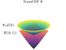
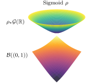
Figure 10: Illustration of the statistical manifolds of the pushforward Gaussian distributions $\mathcal{G}(\mathbb{R})$ through the normCDF and the sigmoid respectively compared to the statistical manifold of Beta distributions $\mathcal{B}((0,1))$. NormCDF, unlike the sigmoid, makes the manifolds intersect at the point $\Phi_{*}\mathcal{N}(0,1)=B(1,1)$.

Here, we argue that the normCDF activation is an ideal choice for approximating Gaussian pushforwards with Beta distributions by interpreting Figure 10. This extends the work from (MacKay, 1998), as it shows how one can make sense of the ‘right’ basis for performing Laplace approximations in the classification setting.

$\Phi_{*}\mathcal{G}(\mathbb{R})$, $\rho_{*}\mathcal{G}(\mathbb{R})$ the space of pushforwards of Gaussian distributions by normCDF and sigmoid respectively, and $\mathcal{B}((0,1))$, the space of Beta distributions, are statistical manifolds naturally equipped with Riemannian metrics, that is their respective Fisher information metrics. We would like to visualise these manifolds. However, two difficulties arise.

The first difficulty is that, while these manifolds all lie in the infinite-dimensional vector space of signed measures on the open unit interval $\mathcal{M}((0,1))$, there is no subspace $\mathbb{V}\subset\mathcal{M}((0,1))$ which is 3-dimensional ($\mathbb{V}\cong\mathbb{R}^{3}$) and contains any two of these statistical manifolds ($\Phi_{*}\mathcal{G}(\mathbb{R}),\mathcal{B}((0,1))\subset\mathbb{V}$ or $\rho_{*}\mathcal{G}(\mathbb{R}),\mathcal{B}((0,1))\subset\mathbb{V}$). We will work around this by building distinct isometric embeddings $\Phi_{*}\mathcal{G}(\mathbb{R})\hookrightarrow\mathbb{V}$, $\rho_{*}\mathcal{G}(\mathbb{R})\hookrightarrow\mathbb{V}$ and $\mathcal{B}((0,1))\hookrightarrow\mathbb{V}$ for some 3-dimensional vector space $\mathbb{V}$. This means that while the shape of the manifold illustrations is meaningful, the positioning of a manifold with respect to another is not, apart from some design choices that we describe below.

The second difficulty is that some–if not all–of these manifolds cannot be embedded isometrically into Euclidean space. As a workaround, we instead embed them into the 3-dimensional Minkowski space $\mathbb{R}^{2,1}$, that is $\mathbb{R}^{3}$ equipped with the pseudo-Riemannian metric $dx_{1}^{2}+dx_{2}^{2}-dx_{3}^{2}$.

The key observation is that $\Phi_{*}\mathcal{G}(\mathbb{R})$ and $\rho_{*}\mathcal{G}(\mathbb{R})$ are isometric to $\mathcal{G}(\mathbb{R})$. This is because $\Phi$ and $\rho$ are diffeomorphisms, so in particular sufficient statistics, and the Fisher information metric is invariant under sufficient statistics (Ay et al., 2017, Section 5.1.3). Visually, this means that $\varphi_{*}\mathcal{G}(\mathbb{R})$ has the same shape irrespectively of the diffeomorphism activation function $\varphi$. One can thus observe that, given that $\mathcal{B}((0,1))$ is not isometric to $\mathcal{G}(\mathbb{R})$, there exists no activation $\varphi$ such that $\varphi_{*}\mathcal{G}(\mathbb{R})=\mathcal{B}((0,1))$. To design an activation $\varphi$ that maps Gaussians to Betas, the best one can hope to do is to map one specific Gaussian distribution $\mathcal{N}(\mu,\sigma^{2})$ to a specific Beta distribution $B(\alpha,\beta)$. This is done with the map $F_{\alpha,\beta}^{-1}\circ\Phi_{\mu,\sigma^{2}}$ where $\Phi_{\mu,\sigma^{2}}$ and $F_{\alpha,\beta}$ are the cumulative distribution functions of $\mathcal{N}(\mu,\sigma^{2})$ and $B(\alpha,\beta)$ respectively. Taking $\mu=0$, $\sigma^{2}=1$, $\alpha=\beta=1$ we get $\Phi_{0,1}=\Phi$ and $F_{1,1}=\operatorname{id}_{(0,1)}$, yielding $F_{\alpha,\beta}^{-1}\circ\Phi_{\mu,\sigma^{2}}=\Phi$.

Now $\mathcal{G}(\mathbb{R})$, and hence $\Phi_{*}\mathcal{G}(\mathbb{R})$ and $\rho_{*}\mathcal{G}(\mathbb{R})$, is isometric to the hyperbolic plane Ay et al. (2017, Example 3.1). We can embed this isometrically into Minkowski space with the classical hyperboloid model of the hyperbolic plane (Reynolds, 1993),

$$\mathcal{G}(\mathbb{R})\hookrightarrow\mathbb{R}^{2,1}.$$ (58)

For $\mathcal{B}((0,1))$, we use the isometric embedding from Le Brigant et al. (2021, Proposition 2):

$$\mathcal{B}((0,1)) \hookrightarrow\mathbb{R}^{2,1}$$ (59)

$$(\alpha,\beta) \mapsto(\eta(\alpha),\eta(\beta),\eta(\alpha+\beta))$$

where $\eta(a):=\int_{1}^{a}\sqrt{\psi^{\prime}(r)}\;dr$ and $\psi$ is the digamma function.

Finally, we choose our embedding Equation 58 for $\Phi_{*}\mathcal{G}(\mathbb{R})$ such that it intersects the embedding Equation 59 at a point, to highlight that the statistical manifolds $\Phi_{*}\mathcal{G}(\mathbb{R})$ and $\mathcal{B}((0,1))$ intersect at a point in the infinite-dimensional ambient space $\mathcal{M}((0,1))$, while $\rho_{*}\mathcal{G}(\mathbb{R})$ and $\mathcal{B}((0,1))$ do not.

Moreover, since $\Phi_{*}\mathcal{N}(0,1)=B(1,1)$, our moment matching approximation Equation 56 is exact when $\mathrm{f}(x)$ is the standard Normal distribution.

Appendix E Comparison with the Energy Model View of Classifiers

Grathwohl et al. (2019) propose to view classifiers of the form Equation 2 as energy-based models by

$$p(c\mid x) =\frac{\exp(f_{c}(x))}{\sum_{c^{\prime}=1}^{C}\exp(f_{c^{\prime}}(x))},$$ (60)

$$p(x,c) =\frac{\exp(f_{c}(x))}{Z},$$

$$p(x) =\frac{\sum_{c=1}^{C}\exp(f_{c}(x))}{Z}$$

where $Z=\int_{\mathcal{X}}\sum_{c=1}^{C}\exp(f_{c}(x))\;dx$. Note the consistency

$$p(c\mid x)=\frac{p(x,c)}{p(x)}.$$ (61)

Observe that the choice of $p(x,c)$ and $p(x)$ in Equation 60 is not canonical: we could have multiplied $p(x,c)$ and $p(x)$ by $\frac{h(x)}{Z^{\prime}}$ for any non-vanishing function $h$ and appropriate normalisation constant $Z^{\prime}$, and we would still obtain the consistency Equation 61. Grathwohl et al. (2019) propose to use the degree of freedom in the logits to train for Equation 60, turning discriminative models into generative models.

Note that $\exp$ in Equation 60 can be replaced by any positive activation $\varphi$. In our framework, we train for $\sum_{c=1}^{C}\varphi(f_{c}(x))=s(x)$. More specifically, in the present work, we train for $\sum_{c=1}^{C}\varphi(f_{c}(x))=1$ (Section 4), making use of the degree of freedom in the logits to obtain exact predictives in Equation 13. In the formalism Equation 60, this means we are setting $x$ to be uniformly distributed. An interesting avenue of future research would be to combine our framework with that of Grathwohl et al. (2019), by e.g. training for $\sum_{c=1}^{C}\varphi(f_{c}(x))\propto p(x)$, and extending the framework of Grathwohl et al. (2019) to second-order distributions.

Appendix F List of Predictive and Dirichlet Parameters Formulas

F.1 Predictive Formulas

We gather formulas for all predictive estimators $\bm{\hat{p}}$ of the true predictive $\mathbb{E}_{\bm{P}\sim\bm{a}_{*}\mathcal{N}(\bm{\mu},\bm{\Sigma})}[\bm{P}]$, $\bm{\Sigma}=\bm{\operatorname{\mathbf{diag}}}(\bm{\sigma}^{2})$, used in our experiments (Section 6).

F.1.1 Softmax

Monte Carlo

One can Monte Carlo estimate the true predictive as follows:

$$\bm{\hat{p}}:=\frac{1}{S}\sum_{s=1}^{S}\bm{\hat{p}}^{(s)}$$ (62)

where the $\bm{\hat{p}}^{(s)}$ are sampled i.i.d. from $\mathcal{N}(\bm{\mu},\bm{\Sigma})$.

Mean Field (Section A.4)

The Mean Field predictive (Lu et al., 2021) uses the following approximation for the true predictive:

$$\bm{\hat{p}}:=\bm{\operatorname{\mathbf{softmax}}}\left(\frac{\bm{\mu}}{\sqrt{1+\frac{\pi}{8}\bm{\sigma}^{2}}}\right).$$ (63)

Laplace Bridge

The Laplace Bridge predictive (Hobbhahn et al., 2022) approximates the true predictive as follows:

$$\bm{\hat{p}}:=\frac{\frac{1}{\bm{\tilde{\sigma}}^{2}}\left(1-\frac{2}{C}+\frac{e^{\bm{\tilde{\mu}}}}{C^{2}}\sum_{c=1}^{C}e^{-\tilde{\mu}_{c}}\right)}{\sum_{c=1}^{C}\frac{1}{\tilde{\sigma}^{2}_{c}}\left(1-\frac{2}{C}+\frac{e^{\bm{\tilde{\mu}}}}{C^{2}}\sum_{c^{\prime}=1}^{C}e^{-\tilde{\mu}_{c^{\prime}}}\right)}$$ (64)

where

$$\bm{\tilde{\mu}}^{2}:=\sqrt{\frac{\sqrt{C/2}}{\sum_{c=1}^{C}\sigma^{2}_{c}}}\bm{\mu},\;\bm{\tilde{\sigma}^{2}}:=\frac{\sqrt{C/2}}{\sum_{c=1}^{C}\sigma^{2}_{c}}\bm{\sigma}^{2}.$$ (65)

F.1.2 Exp

Our analytic predictive for the exp activation function (Section 2.1) is given by

$$\bm{\hat{p}}:=\frac{\bm{\exp}\left(\bm{\mu}+\frac{\bm{\sigma}^{2}}{2}\right)}{\sum_{c=1}^{C}\exp\left(\mu_{c}+\frac{\sigma^{2}_{c}}{2}\right)}.$$ (66)

F.1.3 NormCDF

The analytic predictive for the normCDF activation function (Section 2.2) is computed as

$$\bm{\hat{p}}:=\frac{\bm{\Phi}\left(\frac{\bm{\mu}}{\sqrt{1+\bm{\sigma}^{2}}}\right)}{\sum_{c=1}^{C}\Phi\left(\frac{\mu_{c}}{\sqrt{1+\sigma^{2}_{c}}}\right)}.$$ (67)

F.1.4 Sigmoid

For the sigmoid activation function (Section 2.2), the analytic predictive can be computed as

$$\bm{\hat{p}}:=\frac{\bm{\rho}\left(\frac{\bm{\mu}}{\sqrt{1+\frac{\pi}{8}\bm{\sigma}^{2}}}\right)}{\sum_{c=1}^{C}\rho\left(\frac{\mu_{c}}{\sqrt{1+\frac{\pi}{8}\sigma^{2}_{c}}}\right)}.$$ (68)

F.2 Dirichlet Parameters Formulas

We now gather the formulas of the parameters $\bm{\gamma}$ for the Dirichlet approximations to the Gaussian pushforwards.

F.2.1 Softmax

The Laplace Bridge method (Hobbhahn et al., 2022) uses the following Dirichlet parameters:

$$\bm{\gamma}:=\frac{1}{\bm{\tilde{\sigma}}^{2}}\left(1-\frac{2}{C}+\frac{e^{\bm{\tilde{\mu}}}}{C^{2}}\sum_{c=1}^{C}e^{-\tilde{\mu}_{c}}\right)$$ (69)

where

$$\bm{\tilde{\mu}}^{2}:=\sqrt{\frac{\sqrt{C/2}}{\sum_{c=1}^{C}\sigma^{2}_{c}}}\bm{\mu},\;\bm{\tilde{\sigma}^{2}}:=\frac{\sqrt{C/2}}{\sum_{c=1}^{C}\sigma^{2}_{c}}\bm{\sigma}^{2}.$$ (70)

F.2.2 Exp

Exp uses the analytic parameters derived from Moment Matching the Gaussian pushforwards (Section 3.1):

$$\bm{\gamma}:=\left(\prod_{c=1}^{C}\frac{a_{c}\cdot\max(\sum_{c^{\prime}=1}^{C}a_{c^{\prime}},1)-b_{c}}{b_{c}-a_{c}^{2}}\right)^{1/C}\frac{\bm{a}}{\sum_{c=1}^{C}a_{c}}$$ (71)

where

$$\bm{a}=\exp\left(\bm{\mu}+\frac{\bm{\sigma}^{2}}{2}\right),\;\bm{b}=\exp(2\bm{\mu}+2\bm{\sigma}^{2}).$$ (72)

F.2.3 NormCDF

NormCDF uses the analytic parameters derived from Moment Matching the Gaussian pushforwards (Section 3.1):

$$\bm{\gamma}:=\left(\prod_{c=1}^{C}\frac{a_{c}\cdot\max(\sum_{c^{\prime}=1}^{C}a_{c^{\prime}},1)-b_{c}}{b_{c}-a_{c}^{2}}\right)^{1/C}\frac{\bm{a}}{\sum_{c=1}^{C}a_{c}}$$ (73)

where

$$\bm{a}=\bm{\Phi}\left(\frac{\bm{\mu}}{\sqrt{1+\bm{\sigma}^{2}}}\right),\;\bm{b}=\bm{\Phi}\left(\frac{\bm{\mu}}{\sqrt{1+\bm{\sigma}^{2}}}\right)-2\bm{T}\left(\frac{\bm{\mu}}{\sqrt{1+\bm{\sigma}^{2}}},\frac{1}{\sqrt{1+2\bm{\sigma}^{2}}}\right).$$ (74)

F.2.4 Sigmoid

Sigmoid uses the analytic parameters derived from Moment Matching the Gaussian pushforwards (Section 3.1):

$$\bm{\gamma}:=\left(\prod_{c=1}^{C}\frac{a_{c}\cdot\max(\sum_{c^{\prime}=1}^{C}a_{c^{\prime}},1)-b_{c}}{b_{c}-a_{c}^{2}}\right)^{1/C}\frac{\bm{a}}{\sum_{c=1}^{C}a_{c}}$$ (75)

where

$$\bm{a}=\bm{\rho}\left(\frac{\bm{\mu}}{\sqrt{1+\frac{\pi}{8}\bm{\sigma}^{2}}}\right),\;\bm{b}=\bm{\rho}\left(\frac{\bm{\mu}}{\sqrt{1+\frac{\pi}{8}\bm{\sigma}^{2}}}\right)-\frac{1}{\sqrt{1+\frac{\pi}{8}\bm{\sigma}^{2}}}\bm{\rho}\left(\frac{\bm{\mu}}{\sqrt{1+\frac{\pi}{8}\bm{\sigma}^{2}}}\right)\left(1-\bm{\rho}\left(\frac{\bm{\mu}}{\sqrt{1+\frac{\pi}{8}\bm{\sigma}^{2}}}\right)\right).$$ (76)

Appendix G List of Uncertainty Estimators

In this section, we list the uncertainty estimators used in our experiments (Section 6).

G.1 Predictive

Given a predictive $\bm{p}$, we consider two uncertainty estimators.

Maximum Probability

$$\operatorname*{arg\,max}_{c\in\{1,\dots C\}}p_{c}.$$ (77)

Entropy

$$-\sum_{c=1}^{C}p_{c}\log p_{c}.$$ (78)

G.2 Monte Carlo

Given $S$ Monte Carlo samples $\bm{\hat{p}}^{(1)},\dots,\bm{\hat{p}}^{(S)}$ with mean $\bm{\hat{p}}$, one can calculate a predictive as their average and derive the estimators in Section G.1. However, Monte Carlo samples allow one to calculate two additional estimators detailed below.

Expected Entropy

$$-\frac{1}{S}\sum_{s=1}^{S}\sum_{c=1}^{C}\hat{p}^{(s)}_{c}\log\hat{p}^{(s)}_{c}.$$ (79)

Mutual Information/Jensen-Shannon Divergence

$$-\sum_{c=1}^{C}{\hat{p}}_{c}\log{\hat{p}}_{c}+\frac{1}{S}\sum_{s=1}^{S}\sum_{c=1}^{C}\hat{p}^{(s)}_{c}\log\hat{p}^{(s)}_{c}.$$ (80)

G.3 Dirichlet

Given a second-order Dirichlet distribution with parameters $\bm{\gamma}$, one can obtain the expected entropy and mutual information estimators without the need for Monte Carlo samples.

Expected Entropy

$$-\sum_{c=1}^{C}\frac{\gamma_{c}}{\sum_{c^{\prime}=1}^{C}\gamma_{c^{\prime}}}\left(\psi(\gamma_{c}+1)-\psi\left(\sum_{c^{\prime}=1}^{C}\gamma_{c^{\prime}}+1\right)\right)$$ (81)

where $\psi$ is the digamma function.

Mutual Information

$$\sum_{c=1}^{C}\frac{\gamma_{c}}{\sum_{c^{\prime}=1}^{C}\gamma_{c^{\prime}}}\left(-\log\gamma_{c}+\log\left(\sum_{c^{\prime}=1}^{C}\gamma_{c^{\prime}}\right)+\psi(\gamma_{c}+1)-\psi\left(\sum_{c^{\prime}=1}^{C}\gamma_{c^{\prime}}+1\right)\right).$$ (82)

Appendix H Experimental Setup

This section describes our experimental setup in detail.

We have two main research questions:

• What are the effects of changing the learning objective?

• Do we have to sacrifice performance for sample-free predictives?

To answer the first question, we evaluate our analytic predictives (Sigmoid, NormCDF, Exp) and moment-matched Dirichlet distributions against softmax models equipped with approximate inference tools (Laplace Bridge (Hobbhahn et al., 2022), Mean Field (Lu et al., 2021), Monte Carlo sampling). We consider Heteroscedastic Classifiers (HET) (Collier et al., 2021), Spectral-Normalized Gaussian Processes (SNGP) (Liu et al., 2020), and last-layer Laplace approximation methods (Daxberger et al., 2021) as backbones (see Appendix J for details).

The resulting 18 (method, activation, predictive) triplets are evaluated on ImageNet-1k (Deng et al., 2009) and CIFAR-10 (Krizhevsky & Hinton, 2009) on five metrics aligning with practical needs from uncertainty estimates (Mucsányi et al., 2023):

1. Log probability proper scoring rule for the predictive,

2. Expected calibration error of the predictive’s maximum-probability confidence,

3. Binary log probability proper scoring rule for the correctness prediction task,

4. Accuracy of the predictive’s argmax,

5. AUROC for the out-of-distribution (OOD) detection task.

See Appendix I for details.

For ImageNet, we treat ImageNet-C (Hendrycks & Dietterich, 2019) samples with 15 corruption types and 5 severity levels as OOD samples. For CIFAR-10, we use the CIFAR-10C corruptions.

For the second question, we consider fixed (method, activation) pairs and test whether our methods perform on par with the Monte Carlo sampled predictives.

To provide a fair comparison, we reimplement each method as simple-to-use wrappers around deterministic backbones.

For ImageNet evaluation, we use a ResNet-50 backbone pretrained with the softmax activation function, and train each (method, activation) pair for 50 ImageNet-1k epochs following Mucsányi et al. (2024). We train with the LAMB optimizer (You et al., 2019) using a batch size of $128$ and gradient accumulation across $16$ batches, resulting in an effective batch size of $2048$, following Tran et al. (2022). We further use a cosine learning rate schedule with a single warmup epoch using a warmup learning rate of $0.0001$. The learning rate is treated as a hyperparameter and selected from the interval $[0.0005,0.05]$ based on the validation performance. The weight decay is selected from the set $\{0.01,0.02\}$. During training, we keep track of the best-performing checkpoint on the validation set and load it before testing. We search for ideal hyperparameters with a ten-step Bayesian Optimization scheme (Shahriari et al., 2015) in Weights & Biases (Biewald, 2020) based on the negative log-likelihood.

On CIFAR-10, we train ResNet-28 models from scratch for 100 epochs. The only exceptions are the SNGP models that are trained for 125 epochs (Liu et al., 2020). We train with Momentum SGD using a batch size of $128$ and no gradient accumulation. Similarly to ImageNet, we use a cosine learning rate schedule but with five warmup epochs and warmup learning rate $1\mathrm{e}{-5}$. The learning rate is also treated as a hyperparameter on CIFAR-10. We use the interval $[0.05,1]$ for Sigmoid and NormCDF, and $[0.01,0.15]$ for Softmax and Exp. The optimal learning rates for Sigmoid and NormCDF are generally larger, as the class-wise binary cross-entropies are averaged instead of summed. The weight decay is selected from the interval $[1\mathrm{e}{-6},1\mathrm{e}{-4}]$. Similarly to ImageNet, we use the best-performing checkpoint in the tests and use a ten-step Bayesian Optimization scheme to select performant hyperparameters.

Appendix I Benchmark Metrics

Our experiments use five tasks/metrics:

1. Log probability proper scoring rule for the predictive,

2. Expected calibration error of the predictive’s maximum-probability confidence,

3. Binary log probability proper scoring rule for the correctness prediction task,

4. Accuracy of the predictive’s argmax,

5. AUROC for the out-of-distribution detection task.

Below, we describe these metrics and their respective tasks.

I.1 Log Probability Proper Scoring Rule for the Predictive

First, we briefly discuss proper and strictly proper scoring rules over general probability measures based on (Mucsányi et al., 2023).

Consider a function $S\colon\mathcal{Q}\times\mathcal{Y}\to\mathbb{R}$ where $\mathcal{Q}$ is a family of probability distributions over the space $\mathcal{Y}$, called the label space.

$S$ is called a proper scoring rule if and only if

$$\max_{q\in\mathcal{Q}}\mathbb{E}_{Y\sim p}S(q,Y)=\mathbb{E}_{Y\sim p}S(p,Y),$$ (83)

i.e., $p$ is one of the maximisers of $S$ in $q$ in expectation. $S$ is further strictly proper if $\operatorname*{arg\,max}_{q\in\mathcal{Q}}\mathbb{E}_{Y\sim p}S(q,Y)=p$ is the unique maximiser of $S$ in $q$ in expectation.

The log probability scoring rule for categorical distributions is defined as

$$S(q,c)=\sum_{c^{\prime}=1}^{C}\delta_{c,c^{\prime}}\log q_{c^{\prime}}(x)=\log q_{c}(x),$$ (84)

where $c\in\{1,\dotsc,C\}$ is the true class and $\delta$ is the Kronecker delta. $S$ defined this way is a strictly proper scoring rule, i.e. $\mathbb{E}_{Y\sim p}S(q,Y)$ is maximal if and only if

$$q(Y=c\mid x)=p(Y=c\mid x)\;\forall c\in\{1,\dotsc,C\}.$$ (85)

The score above is equivalent to the negative cross-entropy loss.

I.2 Expected Calibration Error

To set up the required quantities for the Expected Calibration Error (ECE) metric (Naeini et al., 2015), we follow the steps below, based on (Mucsányi et al., 2023).

1. Train a neural network on the training dataset.

2. Create predictions and confidence estimates on the test data.

3. Group the predictions into $M$ bins based on the confidences estimates. Define bin $B_{m}$ to be the set of all indices $n$ of predictions $(\hat{y}_{n},\tilde{c}_{n})$ for which

   $$\tilde{c}_{n}\in\left(\frac{m-1}{M},\frac{m}{M}\right].$$ (86)

The Expected Calibration Error (ECE) metric (Naeini et al., 2015) is then defined as

$$\mathrm{ECE}=\sum_{m=1}^{M}\frac{|B_{m}|}{n}\left|\mathrm{acc}(B_{m})-\mathrm{conf}(B_{m})\right|$$ (87)

where

$$\mathrm{acc}(B_{m}) =\frac{1}{|B_{m}|}\sum_{n\in B_{m}}1\left(\hat{y}_{n}=c_{n}\right),$$ (88)

$$\mathrm{conf}(B_{m}) =\frac{1}{|B_{m}|}\sum_{n\in B_{m}}\max_{c\in\{1,\dotsc,C\}}f_{c}(x_{n}).$$ (89)

Intuitively, the ECE is high when the model’s per-bin confidences match its accuracy on the bin. We use $M=15$ bins in this paper.

I.3 Binary Log Probability Proper Scoring Rule for Correctness Prediction

The correctness prediction task measures the models’ ability to predict the correctness of their own predictions. We consider correctness estimators $\tilde{c}(x)\in[0,1]$ for inputs $x\in\mathcal{X}$ derived from the predictives. Framed as a binary prediction task, the goal of these estimators is to predict the probability of the predicted class’ correctness. In particular, for an (input, target) pair $(x,y)$ with $x\in\mathcal{X},y\in\mathcal{Y}$, we set the correctness target to

$$\ell\equiv\ell(x,y)=1\left(\max_{c\in\{1,\dotsc,C\}}h_{c}(x)=y\right).$$ (90)

Dropping the dependency on $x\in\mathcal{X}$ for brevity, the log probability score for binary targets $\ell\in\{0,1\}$ and estimators $\tilde{c}\in[0,1]$ is defined as

$$S(\tilde{c},\ell)=\begin{cases}\log c&\mathrm{if}\ \ell=1\\ \log(1-\tilde{c})&\mathrm{if}\ \ell=0\end{cases}=\ell\log\tilde{c}+(1-\ell)\log(1-\tilde{c}).$$ (91)

One can show that this is indeed a strictly proper scoring rule (Mucsányi et al., 2023).

I.4 Accuracy

For completeness, the accuracy of a predictive $h$ on a dataset $(x_{n},c_{n})_{n=1}^{N}$ is

$$\operatorname{acc}(h;(x_{n},c_{n})_{n=1}^{N})=\frac{1}{N}\sum_{n=1}^{N}1\left(\operatorname*{arg\,max}_{c\in\{1,\dotsc,C\}}h_{c}(x_{n})=\tilde{c}_{n}\right).$$ (92)

I.5 Area Under the Receiver Operating Characteristic Curve for Out-of-Distribution Detection

Out-of-distribution detection is another binary prediction task where a general uncertainty estimator $u(x)\in\mathbb{R}$ (derived from predictives or second-order Dirichlet distributions) is tasked to separate ID and OOD samples from a balanced mixture. The target OOD indicator variable $o(x)$ is, therefore, binary. As the uncertainty estimator can take on any real value, we measure the Area Under the Receiver Operating Characteristic curve (AUROC), which quantifies the separability of ID and OOD samples w.r.t. the uncertainty estimator.

Given uncertainty estimates $u_{n}\equiv u(x_{n})$ and target binary labels $o_{i}$ on a balanced dataset $(x_{n},o_{n})_{n=1}^{N}$, as well as a threshold $t\in\mathbb{R}$, we predict $1$ (out-of-distribution) when $u_{n}\geq t$ and $0$ (in-distribution) when $u_{n}<t$. This lets us define the following index sets:

$$\text{True positives: }\mathrm{TP}(t) =\left\{n:o_{n}=1\land u_{n}\geq t\right\}$$

$$\text{False positives: }\mathrm{FP}(t) =\left\{n:o_{n}=0\land u_{n}\geq t\right\}$$

$$\text{False negatives: }\mathrm{FN}(t) =\left\{n:o_{n}=1\land u_{n}<t\right\}$$

$$\text{True negatives: }\mathrm{TN}(t) =\left\{n:o_{n}=0\land u_{n}<t\right\}.$$

The Receiver Operating Characteristic (ROC) curve compares the following quantities:

$$\mathrm{TPR}(t) =\frac{|\mathrm{TP}(t)|}{|\mathrm{TP}(t)|+|\mathrm{FN}(t)|}=\frac{|\mathrm{TP}(t)|}{|\mathrm{P}|}$$

$$\mathrm{FPR}(t) =\frac{|\mathrm{FP}(t)|}{|\mathrm{FP}(t)|+|\mathrm{TN}(t)|}=\frac{|\mathrm{FP}(t)|}{|\mathrm{N}|}.$$

Here, FPR tells us how many of the actual negative samples in the dataset are recalled (predicted positive) at threshold $t$.

One can draw a curve of $(\mathrm{FPR}(t),\mathrm{TPR}(t))$ for all $t$ from $-\infty$ to $+\infty$. This is the ROC curve. The area under this curve quantifies how well the uncertainty estimator $u(x)$ can separate in-distribution and out-of-distribution inputs.

Appendix J Benchmarked Methods

This section describes our benchmarked methods and provides further implementation details.

J.1 Spectral Normalized Gaussian Process

Spectral normalized Gaussian processes (SNGP) (Liu et al., 2020) use spectral normalization of the parameter tensors for distance-awareness and a last-layer Gaussian process approximated by Fourier features to capture uncertainty. For an input $x\in\mathcal{X}$ and number of classes $C$, they predict a $C$-variate Gaussian distribution

$$\mathcal{N}\left(\bm{B}\bm{\phi}(x),\bm{\phi}(x)^{\top}\left(\bm{\Psi}^{\top}\bm{\Psi}+\bm{I}\right)^{-1}\bm{\phi}(x)\bm{I}_{C}\right),$$ (93)

in logit space.

• $\bm{B}\in\mathbb{R}^{C\times D}$ is a learned parameter matrix that maps pre-logits to logits.

• $\bm{\phi}(x)=\bm{\cos}\left(\bm{W}\bm{f}^{L-1}(x)+\bm{b}\right)\in\mathbb{R}^{D}$ is a random pre-logit embedding of the input $x\in\mathcal{X}$. $\bm{f}^{L-1}(x)$ denotes the pre-logit embedding. $\bm{W}$ is a fixed semi-orthogonal random matrix, and $\bm{b}$ is also a fixed random vector but sampled from $\text{Uniform}(0,2\pi)$.

• $\bm{\Psi}^{\top}\bm{\Psi}$ is the (unnormalised) empirical covariance matrix of the pre-logits of the training set. This is calculated via accumulating the mini-batch estimates during the last epoch.

The method applies spectral normalization to the hidden weights in each layer using a power iteration scheme with a single iteration per batch to obtain the largest singular value. Liu et al. (2020) claim this helps with input distance awareness.

J.2 Heteroscedastic Classifier

Heteroscedastic classifiers (HET) (Collier et al., 2021) construct a Gaussian distribution in the logit space to model per-input uncertainties:

$$\mathcal{N}(\bm{f}(x),\bm{\Sigma}(x)),$$ (94)

where $\bm{f}(x)\in\mathbb{R}^{D}$ is the logit mean for input $x\in\mathcal{X}$ and

$$\bm{\Sigma}(x)=\bm{V}(x)^{\top}\bm{V}(x)+\bm{\operatorname{\mathbf{diag}}}(\bm{d}(x))$$ (95)

is a (positive definite) covariance matrix. Both the low-rank term $\bm{V}(x)$ and the diagonal term $\bm{d}(x)$ are calculated as a linear function of the pre-logit layer’s output.

To learn the per-input covariance matrices from the training set, one has to construct a predictive estimate from $\mathcal{N}(\bm{f}(x),\bm{\Sigma}(x))$ using any of the methods in Appendix F. This predictive estimate is then trained using a standard cross-entropy (NLL) loss.

HET uses a temperature parameter to scale the logits before calculating the BMA. This is chosen using a validation set.

In Section 2.3, we show that when our constraint is satisfied, the off-diagonal terms of the covariance matrix do not matter for the predictive. This means that, in our framework, one can discard the low-rank term $\bm{V}(x)$ and only model the diagonal term $\bm{d}(x)$ without a decrease in expressivity. To keep comparisons fair and use the same backbone with the same number of parameters, we also only model $\bm{d}(x)$ for softmax-based predictives.

J.3 Laplace Approximation

The Laplace approximation (Daxberger et al., 2021) approximates the posterior $p(\bm{\theta}\mid\mathcal{D})$ over the network parameters $\bm{\theta}$ for a Gaussian prior $p(\bm{\theta})$ and likelihood defined by the network architecture by a Gaussian. In its simplest form, it uses the maximum a posteriori (MAP) weights $\bm{\theta}_{\text{MAP}}\in\mathbb{R}^{P}$ as the mean and the inverse Hessian of the regularized loss over the training set $\tilde{\mathcal{L}}(\bm{\theta};\mathcal{D})=\mathcal{L}(\bm{\theta};\mathcal{D})+\lambda\|\bm{\theta}\|_{2}^{2}$ evaluated at the MAP as the covariance matrix:

$$\mathcal{N}\left(\bm{\theta}_{\text{MAP}},\left(\left.\frac{\partial^{2}\tilde{\mathcal{L}}(\bm{\theta};\mathcal{D})}{\partial\theta_{i}\partial\theta_{j}}\right|_{\bm{\theta}_{\text{MAP}}}\right)^{-1}\right)=\mathcal{N}\left(\bm{\theta}_{\text{MAP}},\left(\left.\frac{\partial^{2}\mathcal{L}(\bm{\theta};\mathcal{D})}{\partial\theta_{i}\partial\theta_{j}}\right|_{\bm{\theta}_{\text{MAP}}}+\lambda\bm{I}_{P}\right)^{-1}\right).$$ (96)

This is a locally optimal post-hoc Gaussian approximation of the true posterior $p(\bm{\theta}\mid\mathcal{D})$ based on a second-order Taylor approximation. For details, see (Tatzel et al., 2025).

For deep neural networks, the Hessian matrix is often replaced with the Generalized Gauss-Newton (GGN) matrix. The GGN is guaranteed to be positive semidefinite even for suboptimal weights and has efficient approximation schemes, such as Kronecker-Factored Approximate Curvature (Martens & Grosse, 2015) or low-rank approximations.

Denoting our curvature estimate of choice by $\bm{G}$, the logit-space Gaussian is obtained by pushing forward the weight-space Gaussian measure through the linearised model around $\bm{\theta}_{\text{MAP}}$. For an input $x\in\mathcal{X}$, this results in

$$\mathcal{N}\left(\left(\bm{J}_{\bm{\theta}_{\text{MAP}}}\bm{f}(x)\right)\bm{\theta}_{\text{MAP}},\left(\bm{J}_{\bm{\theta}_{\text{MAP}}}\bm{f}(x)\right)\left(\bm{G}+\lambda\bm{I}_{P}\right)^{-1}\left(\bm{J}_{\bm{\theta}_{\text{MAP}}}\bm{f}(x)\right)^{\top}\right),$$ (97)

where $\bm{J}_{\bm{\theta}_{\text{MAP}}}\bm{f}(x)\in\mathbb{R}^{C\times P}$ is the model Jacobian matrix.

We use a last-layer KFAC Laplace variant in our experiments and use the full training set for calculating the GGN instead of a mini-batch based on recent works on the bias in mini-batch estimates (Tatzel et al., 2025).

Appendix K CIFAR-10 Experiments

This appendix section repeats the experiments presented in the main paper on the CIFAR-10 dataset. For a detailed description of the experimental setup, refer to Appendix H. Appendix I describes the used tasks and metrics.

As stated in the main paper, our two research questions are:

• What are the effects of changing the learning objective? (Section K.2)

• Do we have to sacrifice performance for sample-free predictives? (Section K.1)

K.1 Quality of Sample-Free Predictives

Table 2: Comparison of ECE results for different predictives using a fixed Laplace backbone.

Method	Mean	Std
Softmax Laplace
MC 100	0.0096	0.0013
MC 1000	0.0102	0.0016
MC 10	0.0120	0.0013
Mean Field	0.0121	0.0029
Laplace Bridge Predictive	0.5933	0.0105
NormCDF Laplace
Analytic	0.0074	0.0012
MC 1000	0.0092	0.0022
MC 100	0.0095	0.0015
MC 10	0.0100	0.0020

Similarly to the main paper, in this section, we investigate our first research question: whether there is a price to pay for sample-free predictives. Table 2 showcases the two best-performing (activation, method) pairs on the ECE metric and the CIFAR-10 dataset: Softmax and NormCDF Laplace. Mean Field (MF) is a strong alternative for sample-free predictives, but it has no guarantees and can fall behind MC sampling (see also Figure 1). When the constraint is satisfied, the analytic NormCDF predictive is exact. Empirically, our analytic predictives always perform on par with MC sampling.

K.2 Effects of Changing the Learning Objective

As in the main paper, in this section, we use the best-performing predictive and estimator (see Appendix F) for softmax models and employ our methods with the analytic predictives.

K.2.1 Calibration and Proper Scoring

We first evaluate calibration using the log probability scoring rule (Gneiting & Raftery, 2007) and the Expected Calibration Error (ECE) metric (Naeini et al., 2015). Figure 5 shows that on CIFAR-10, the score of our analytic predictives with implicit constraints (Sigmoid, NormCDF) are consistently better than the corresponding softmax results for all methods.

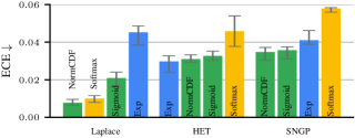
Figure 11: CIFAR-10 ECE results. Analytic predictives with implicit ( ) or explicit ( ) constraints outperform Softmax ( ) on HET and SNGP. Laplace tunes its hyperparameters based on the ECE metric – NormCDF Laplace is the overall best method. Note the restricted $y$-limits for readability.

Figure 11 shows that on CIFAR-10, our analytic predictives have a clear advantage on HET and SNGP. Laplace is a post-hoc method that tunes its hyperparameters on the ECE metric, hence its enhanced performance. Our NormCDF predictive is on par with Softmax.

K.2.2 Correctness Prediction

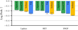
Figure 12: CIFAR-10 log probability proper scoring results for the binary correctness prediction task. Analytic predictives with implicit ( ) constraints consistently outperform Softmax ( ) on all methods.

Figure 12 shows that on the correctness prediction task, our analytic predictives with implicit constraints outperform all Softmax predictives across all methods, as measured by the log probability proper scoring rule.

K.2.3 Accuracy

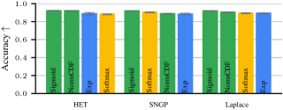
Figure 13: Analytic predictives do not sacrifice accuracy. CIFAR-10 accuracies. Analytic predictives with implicit ( ) or explicit ( ) constraints either outperform or are on par with Softmax ( ) across all methods.

Analytic predictives do not sacrifice accuracy. Figure 13 evidences this claim on CIFAR-10: our analytic predictives either outperform or are on par with Softmax predictives. The most accurate method is Sigmoid HET. These results support the findings of Wightman et al. (2021) that showcase desirable training dynamics of the class-wise cross-entropy loss.

K.2.4 Out-of-Distribution Detection

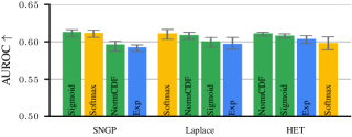
Figure 14: CIFAR-10C OOD detection AUROC results for severity level one. Across all methods, the best-performing predictive is analytic with an implicit constraint ( ).

Finally, we consider the OOD detection task on a balanced mixture of ID (CIFAR-10) and OOD inputs. As OOD inputs, we consider corrupted CIFAR-10C samples. We use the AUROC metric to evaluate the methods’ performance. As shown in Figure 14, the best-performing method is Sigmoid SNGP, an analytic method. Generally, Softmax performs on par with our analytic predictives. Intuitively, separating ID and OOD samples does not require a fine-grained representation of uncertainty, unlike the ECE or proper scoring rules. Nevertheless, the analytic predictives and second-order Dirichlet distributions are considerably cheaper to calculate than Softmax MC predictions (see Section 5).

Appendix L ImageNet Dirichlet Evaluation

This appendix section evaluates our moment-matched Dirichlet distributions on the OOD detection task (Appendix I). Table 3 shows the per-estimator performances of the three best-performing (method, activation) pairs on ImageNet: Sigmoid Laplace, NormCDF HET, and NormCDF Laplace. In all three cases, the best estimator is derived from the moment-matched Dirichlet distributions.

Table 3: Comparison of OOD AUROC results for different uncertainty estimators on the three best-performing (method, activation) pairs: Sigmoid Laplace, NormCDF HET, and NormCDF Laplace. The best estimator is derived from the moment-matched Dirichlet distributions in all three cases.

Method	Mean	Std
Sigmoid Laplace
Dirichlet Mutual Information	0.6388	0.0005
Analytic Predictive Entropy	0.6353	0.0003
MC 1000 Predictive Entropy	0.6323	0.0001
MC 100 Predictive Entropy	0.6323	0.0001
MC 1000 Expected Entropy	0.6321	0.0001
NormCDF HET
Dirichlet Expected Entropy	0.6353	0.0021
MC 1000 Expected Entropy	0.6281	0.0020
MC 100 Expected Entropy	0.6281	0.0020
MC 10 Expected Entropy	0.6281	0.0020
Analytic Predictive Entropy	0.6277	0.0021
NormCDF Laplace
Dirichlet Expected Entropy	0.6321	0.0009
MC 100 Predictive Entropy	0.6296	0.0012
MC 1000 Predictive Entropy	0.6296	0.0012
Closed-Form Predictive Entropy	0.6296	0.0012
MC 10 Predictive Entropy	0.6294	0.0012

Appendix M Further Out-of-Distribution Detection Results

Figure 15 shows OOD detection results across all ImageNet-C severity levels. Our analytic predictives with implicit constraints consistently outperform Softmax.

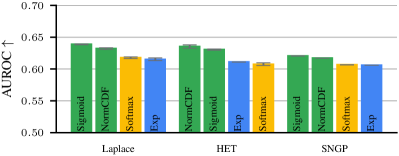
(a) OOD detection AUROC with severity level one.

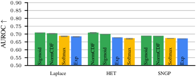
(b) OOD detection AUROC with severity level two.

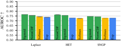
(c) OOD detection AUROC with severity level three.

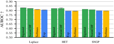
(d) OOD detection AUROC with severity level four.

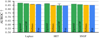
(e) OOD detection AUROC with severity level five.

Figure 15: The OOD detection performance of all methods increases steadily as we increase the severity of the perturbed half of the mixed dataset on the ImageNet validation dataset. Our analytic predictives consistently outperform Softmax.

References

- Atchison & Shen (1980) Atchison, J. and Shen, S. Logistic-normal distributions: Some properties and uses. Biometrika, 67(2):261–272, January 1980. ISSN 0006-3444. doi: 10.1093/biomet/67.2.261. URL https://doi.org/10.1093/biomet/67.2.261.
- Ay et al. (2017) Ay, N., Jost, J., Lê, H. V., and Schwachhöfer, L. Information Geometry, volume 64 of Ergebnisse der Mathematik und ihrer Grenzgebiete 34. Springer International Publishing, Cham, 2017. ISBN 978-3-319-56477-7 978-3-319-56478-4. doi: 10.1007/978-3-319-56478-4. URL http://link.springer.com/10.1007/978-3-319-56478-4.
- Biewald (2020) Biewald, L. Experiment tracking with weights and biases, 2020. URL https://www.wandb.com/. Software available from wandb.com.
- Charpentier et al. (2020) Charpentier, B., Zügner, D., and Günnemann, S. Posterior network: Uncertainty estimation without ood samples via density-based pseudo-counts. Advances in neural information processing systems, 33:1356–1367, 2020.
- Collier et al. (2021) Collier, M., Mustafa, B., Kokiopoulou, E., Jenatton, R., and Berent, J. Correlated input-dependent label noise in large-scale image classification. In Proceedings of the IEEE/CVF conference on computer vision and pattern recognition, pp. 1551–1560, 2021.
- Daganzo (1979) Daganzo, C. Chapter 1 - An Introduction to Disaggregate Demand Modeling in the Transportation Field. In Multinomial Probit, Economic Theory, Econometrics, and Mathematical Economics, pp. 1–29. Academic Press, 1979. ISBN 978-0-12-201150-4. doi: 10.1016/B978-0-12-201150-4.50006-2. URL https://www.sciencedirect.com/science/article/pii/B9780122011504500062.
- Daunizeau (2017) Daunizeau, J. Semi-analytical approximations to statistical moments of sigmoid and softmax mappings of normal variables, March 2017. URL http://arxiv.org/abs/1703.00091. arXiv:1703.00091 [stat].
- Daxberger et al. (2021) Daxberger, E., Kristiadi, A., Immer, A., Eschenhagen, R., Bauer, M., and Hennig, P. Laplace redux-effortless bayesian deep learning. Advances in Neural Information Processing Systems, 34:20089–20103, 2021.
- Deng et al. (2009) Deng, J., Dong, W., Socher, R., Li, L.-J., Li, K., and Fei-Fei, L. Imagenet: A large-scale hierarchical image database. In 2009 IEEE conference on computer vision and pattern recognition, pp. 248–255. Ieee, 2009.
- Depeweg et al. (2018) Depeweg, S., Hernandez-Lobato, J.-M., Doshi-Velez, F., and Udluft, S. Decomposition of uncertainty in bayesian deep learning for efficient and risk-sensitive learning. In International Conference on Machine Learning, pp. 1184–1193. PMLR, 2018.
- Gneiting & Raftery (2007) Gneiting, T. and Raftery, A. E. Strictly proper scoring rules, prediction, and estimation. Journal of the American statistical Association, 102(477):359–378, 2007.
- Grathwohl et al. (2019) Grathwohl, W., Wang, K.-C., Jacobsen, J.-H., Duvenaud, D., Norouzi, M., and Swersky, K. Your classifier is secretly an energy based model and you should treat it like one. In International Conference on Learning Representations, September 2019. URL https://openreview.net/forum?id=Hkxzx0NtDB.
- Hendrycks & Dietterich (2019) Hendrycks, D. and Dietterich, T. Benchmarking neural network robustness to common corruptions and perturbations. arXiv preprint arXiv:1903.12261, 2019.
- Hobbhahn et al. (2022) Hobbhahn, M., Kristiadi, A., and Hennig, P. Fast predictive uncertainty for classification with bayesian deep networks. In Cussens, J. and Zhang, K. (eds.), Proceedings of the Thirty-Eighth Conference on Uncertainty in Artificial Intelligence, volume 180 of Proceedings of Machine Learning Research, pp. 822–832. PMLR, 01–05 Aug 2022. URL https://proceedings.mlr.press/v180/hobbhahn22a.html.
- Hüllermeier & Waegeman (2021) Hüllermeier, E. and Waegeman, W. Aleatoric and epistemic uncertainty in machine learning: An introduction to concepts and methods. Machine learning, 110(3):457–506, 2021.
- Kristiadi et al. (2020) Kristiadi, A., Hein, M., and Hennig, P. Being Bayesian, Even Just a Bit, Fixes Overconfidence in ReLU Networks. In Proceedings of the 37th International Conference on Machine Learning, pp. 5436–5446. PMLR, November 2020. URL https://proceedings.mlr.press/v119/kristiadi20a.html.
- Krizhevsky & Hinton (2009) Krizhevsky, A. and Hinton, G. Learning multiple layers of features from tiny images. Master’s thesis, Department of Computer Science, University of Toronto, 2009.
- Le Brigant et al. (2021) Le Brigant, A., Preston, S. C., and Puechmorel, S. Fisher-Rao geometry of Dirichlet distributions. Differential Geometry and its Applications, 74:101702, February 2021. ISSN 0926-2245. doi: 10.1016/j.difgeo.2020.101702. URL https://www.sciencedirect.com/science/article/pii/S092622452030111X.
- Liu et al. (2020) Liu, J., Lin, Z., Padhy, S., Tran, D., Bedrax Weiss, T., and Lakshminarayanan, B. Simple and principled uncertainty estimation with deterministic deep learning via distance awareness. Advances in Neural Information Processing Systems, 33:7498–7512, 2020.
- Liu et al. (2023) Liu, J. Z., Padhy, S., Ren, J., Lin, Z., Wen, Y., Jerfel, G., Nado, Z., Snoek, J., Tran, D., and Lakshminarayanan, B. A simple approach to improve single-model deep uncertainty via distance-awareness. Journal of Machine Learning Research, 24(42):1–63, 2023. URL http://jmlr.org/papers/v24/22-0479.html.
- Lu et al. (2021) Lu, Z., Ie, E., and Sha, F. Mean-Field Approximation to Gaussian-Softmax Integral with Application to Uncertainty Estimation, May 2021. URL http://arxiv.org/abs/2006.07584. arXiv:2006.07584.
- MacKay (1998) MacKay, D. J. Choice of Basis for Laplace Approximation. Machine Learning, 33(1):77–86, October 1998. ISSN 1573-0565. doi: 10.1023/A:1007558615313. URL https://doi.org/10.1023/A:1007558615313.
- MacKay (1992) MacKay, D. J. C. The Evidence Framework Applied to Classification Networks. Neural Computation, 4(5):720–736, September 1992. ISSN 0899-7667. doi: 10.1162/neco.1992.4.5.720. URL https://ieeexplore.ieee.org/document/6796959. Conference Name: Neural Computation.
- Martens & Grosse (2015) Martens, J. and Grosse, R. Optimizing neural networks with kronecker-factored approximate curvature. In International conference on machine learning, pp. 2408–2417. PMLR, 2015.
- Minka (2000) Minka, T. P. Estimating a Dirichlet distribution, 2000. URL https://tminka.github.io/papers/dirichlet/minka-dirichlet.pdf. Technical Report, MIT.
- Mucsányi et al. (2023) Mucsányi, B., Kirchhof, M., Nguyen, E., Rubinstein, A., and Oh, S. J. Trustworthy machine learning. arXiv preprint arXiv:2310.08215, 2023.
- Mucsányi et al. (2024) Mucsányi, B., Kirchhof, M., and Oh, S. J. Benchmarking uncertainty disentanglement: Specialized uncertainties for specialized tasks. In The Thirty-eight Conference on Neural Information Processing Systems Datasets and Benchmarks Track, 2024. URL https://openreview.net/forum?id=x8RgF2xQTj.
- Mukhoti et al. (2023) Mukhoti, J., Kirsch, A., van Amersfoort, J., Torr, P. H., and Gal, Y. Deep deterministic uncertainty: A new simple baseline. In Proceedings of the IEEE/CVF Conference on Computer Vision and Pattern Recognition, pp. 24384–24394, 2023.
- Naeini et al. (2015) Naeini, M. P., Cooper, G., and Hauskrecht, M. Obtaining well calibrated probabilities using bayesian binning. In Proceedings of the AAAI conference on artificial intelligence, volume 29, 2015.
- Owen (1980) Owen, D. B. A table of normal integrals. Communications in Statistics - Simulation and Computation, January 1980. URL https://www.tandfonline.com/doi/abs/10.1080/03610918008812164.
- Reynolds (1993) Reynolds, W. F. Hyperbolic Geometry on a Hyperboloid. The American Mathematical Monthly, 100(5):442–455, May 1993. ISSN 0002-9890. doi: 10.1080/00029890.1993.11990430. URL https://doi.org/10.1080/00029890.1993.11990430.
- Sensoy et al. (2018) Sensoy, M., Kaplan, L., and Kandemir, M. Evidential deep learning to quantify classification uncertainty. Advances in neural information processing systems, 31, 2018.
- Shahriari et al. (2015) Shahriari, B., Swersky, K., Wang, Z., Adams, R. P., and De Freitas, N. Taking the human out of the loop: A review of bayesian optimization. Proceedings of the IEEE, 104(1):148–175, 2015.
- Spiegelhalter & Lauritzen (1990) Spiegelhalter, D. J. and Lauritzen, S. L. Sequential updating of conditional probabilities on directed graphical structures. Networks, 20(5):579–605, 1990. ISSN 1097-0037. doi: 10.1002/net.3230200507. URL https://onlinelibrary.wiley.com/doi/abs/10.1002/net.3230200507.
- Tatzel et al. (2025) Tatzel, L., Mucsányi, B., Hackel, O., and Hennig, P. Debiasing mini-batch quadratics for applications in deep learning. In The Thirteenth International Conference on Learning Representations, 2025. URL https://openreview.net/forum?id=Q0TEVKV2cp.
- Tran et al. (2022) Tran, D., Liu, J., Dusenberry, M. W., Phan, D., Collier, M., Ren, J., Han, K., Wang, Z., Mariet, Z., Hu, H., et al. Plex: Towards reliability using pretrained large model extensions. arXiv preprint arXiv:2207.07411, 2022.
- Wightman et al. (2021) Wightman, R., Touvron, H., and Jégou, H. ResNet strikes back: An improved training procedure in timm, October 2021. URL http://arxiv.org/abs/2110.00476. arXiv:2110.00476 [cs].
- Wimmer et al. (2023) Wimmer, L., Sale, Y., Hofman, P., Bischl, B., and Hüllermeier, E. Quantifying aleatoric and epistemic uncertainty in machine learning: Are conditional entropy and mutual information appropriate measures? In Uncertainty in Artificial Intelligence, pp. 2282–2292. PMLR, 2023.
- You et al. (2019) You, Y., Li, J., Reddi, S., Hseu, J., Kumar, S., Bhojanapalli, S., Song, X., Demmel, J., Keutzer, K., and Hsieh, C.-J. Large batch optimization for deep learning: Training bert in 76 minutes. arXiv preprint arXiv:1904.00962, 2019.