Heat engines for scale invariant systems dual to black holes

Abstract

According to holography, a black hole is dual to a thermal state in a strongly coupled quantum system. The principle example of holography is the Anti-de Sitter/Conformal Field Theory (AdS/CFT) correspondence. We construct reversible heat engines where the working substance consists of a static thermal equilibrium state of a CFT. For thermal states dual to an asymptotically AdS black hole, this yields a novel realization of Johnson’s holographic heat engines. We compute the efficiency for a number of idealized heat engines, such as the Carnot, Brayton, Otto, Diesel, and Stirling cycles. The efficiency of most heat engines can be derived from the CFT equation of state, which follows from scale invariance, and we compare them to the efficiencies for an ideal gas. However, the Stirling efficiency for a generic CFT is uniquely determined in terms of its characteristic temperature and volume only in the high-temperature or large-volume regime. We derive an exact expression for the Stirling efficiency for CFT states dual to AdS-Schwarzschild black holes, and compare the subleading corrections in the high-temperature regime with those in a generic CFT.

Introduction. Heat engines form a central topic in thermodynamics and played a pivotal role in its historical development [1, 2, 3, 4, 5]. A heat engine consists of a system (working substance) that converts heat into work and operates in a thermodynamic cycle. In a heat engine a certain amount of heat ($Q_{\text{in}}$) is supplied from a heat source to the system, which is then converted into work ($W$) performed by the working substance on a work source, and finally waste heat is expelled from the system ($Q_{\text{out}}$) to a heat sink (we define these three quantities to be positive). The operation of a heat engine is constrained by the first and second law of thermodynamics. The first law, which is nothing but the statement of energy conservation, imposes a constraint on these three quantities: $Q_{\text{in}}=W+Q_{\text{out}}$. The second law imposes a constraint on the efficiency of heat engines that operate between two fixed temperatures. In fact, historically Carnot formulated the first version of the second law in terms of the efficiency of heat engines [6]. The efficiency of a heat engine is defined as the ratio of the work done by the system and the heat supplied into the system:

$$\eta=\frac{W}{Q_{\text{in}}}=1-\frac{Q_{\text{out}}}{Q_{\text{in}}}\,,$$ (1)

where the first law was used to obtain the last expression. According to Carnot’s theorem all heat engines operating between a hot thermal reservoir at temperature $T_{h}$ and a cold thermal reservoir at temperature $T_{c}$ have an efficiency that is less than or equal to that of a reversible engine. Moreover, all reversible engines that operate between two fixed temperatures (where heat exchange only takes places between the system and the heat reservoirs) have the same efficiency that depends only on the temperatures of the reservoirs, called the Carnot efficiency: $\eta_{\text{Carnot}}=1-T_{c}/T_{h}$. The Carnot efficiency thus poses an upper bound to the efficiency of heat engines.

The efficiency of a heat engine is determined by the cyclic path that the system traces in thermodynamic state space, which differs between various engines, as well as by the type of working substance. In textbooks on thermodynamics the ideal gas is typically given as an exemplar for a working system for which the efficiency of idealized heat engines can be computed. However, there are other working systems for which the efficiency of idealized engines can be derived, such as a Van der Waals fluid [7] or a magnetic material [8]. In this work we consider a working substance that consists of a static thermodynamic equilibrium state of a conformal field theory, i.e., a quantum field theory with conformal symmetry.

Our motivation for studying such heat engines comes from holography [9, 10], i.e., the idea that a gravitational theory in a $(D+1)$-dimensional spacetime is equivalent to a quantum gauge theory without gravity living on the $D$-dimensional boundary of the spacetime. The best understood example of such a gauge/gravity duality is the AdS/CFT correspondence [11, 12, 13, 14]. A thermal high-energy state in a holographic CFT living on the (conformal) boundary of asymptotically AdS spacetime is dual to a black hole in the bulk geometry [15, 16]. Therefore, CFT heat engines are a tool to probe black hole physics with a thermodynamic non-gravitational system.

Theorizing about black holes as heat engines [17, 18, 19, 20, 21, 22, 23, 24, 25] and interpreting black hole heat engines in terms of a dual holographic field theory [26, 27, 28, 29] is a common theme in the literature. Particularly, the idea of holographic heat engines has been proposed by Clifford Johnson [26]. Our work may be viewed as a novel realization of this idea, but there are essential differences between Johnson’s heat engines and those in our work. On the one hand, Johnson’s starting point is an extended version of the thermodynamics of black holes in the bulk where the cosmological constant $\Lambda$ is allowed to vary [30, 31, 32, 33, 34] (see [35] for a review). That is, he employs a bulk pressure that is proportional to $\Lambda$ and inversely proportional to Newton’s constant $G$, $P_{\text{bulk}}=-\Lambda/(8\pi G)$, and defines the thermodynamic volume as the conjugate thermodynamic quantity. On the other hand, we construct heat engines in the boundary theory, and define the pressure and volume in the CFT in the standard thermodynamic way. It is important to mention that the bulk pressure is not dual to the CFT pressure. In fact, the bulk pressure corresponds to a central charge $C$ in the CFT or the number of colors $N$ in a large-$N$ $SU(N)$ strongly-coupled gauge theory. It is questionable whether $C$ is a thermodynamic variable, since varying it changes the physical theory [36]. We keep the central charge fixed, so this is not an issue in the present work. Moreover, we stress that even though we define the heat engine in the boundary CFT, there is a one-to-one correspondence between black hole thermodynamics [37, 38, 39, 15] and CFT thermodynamics [16]. In this work we will use the recently developed holographic dictionary in [40, 41, 42, 43] to compute the efficiency for heat engines dual to AdS black holes.

Our aim is to present a novel construction of holographic heat engines and to compute the efficiencies of various idealized engines: Carnot, Brayton, Otto, Diesel, Stirling and the rectangular pressure-volume cycle. We show for most heat engines, except for Stirling, the efficiency is uniquely determined by the CFT equation of state, and is hence the same for holographic and non-holographic CFTs. The Stirling efficiency is only fixed in terms of its characteristic temperature and volume in the high-temperature or large-volume regime, and we compare the subleading corrections in this regime for a generic CFT and for a holographic CFT.

CFT heat engines. We consider heat engines whose working substance consists of a static, global thermodynamic equilibrium state of a CFT in $D$ spacetime dimensions. The working substance of a heat engine traces a thermodynamic cycle, so it returns to its initial state. We assume the thermodynamic cycle consists of quasi-static processes that happen slowly enough so that the system remains in thermal equilibrium at every point in the cycle. This implies that the cycle is reversible. The first law of thermodynamics for quasi-static processes reads

$$\Delta E=Q-P\Delta V\qquad(\text{quasi-static})\,.$$ (2)

Here, $Q$ is positive when it enters the system and negative when it leaves. Moreover, we assumed that other conserved quantities (such as electric charge or angular momentum) are kept fixed. We also do not change the central charge of the CFT during the cycle. Further, in this article we use finite differences $\Delta$, since we take the heat source and sink to be thermal reservoirs, which are so large that heat transfer does not alter their temperature. This permits us to consider finite heat and work transfers instead of infinitesimal transfers.

Moreover, since the cycle is reservible, Clausius’ relation holds for the heat engines under consideration

$$Q=T\Delta S\qquad(\text{reversible})\,.$$ (3)

This implies that isentropic processes are equivalent to adiabatic processes. Hence, we may treat the internal energy as a function of entropy and volume: $E=E(S,V)$, suppressing the dependence on other variables that we keep fixed. We should remark though that the energy and entropy are not extensive for CFTs at finite temperature and in a finite volume, i.e., $E(aS,aV)\neq aE(S,V)$.

For the idealized heat engines that we study the cycle consists of four paths and each path corresponds to a particular thermodynamic process, such as adiabatic $(Q=0)$, isochoric $(\Delta V=0)$, isobaric ($\Delta P=0$), and isothermal ($\Delta T=0$) processes. Depending on the type of processes that constitute the cycle, there are different types of heat engines. We label the vertices of the four paths by $i=1,2,3,4$, and $A_{i}$ denotes the value of the thermodynamic variable $A$ at the $i^{\text{th}}$ vertex.

In order to compute the efficiencies of various CFT heat engines, we will make use of the scale invariance of CFTs. For homogeneous systems, scale invariance implies that the equation of state is $E=(D-1)PV$, often called the conformal equation of state. Note that an ideal gas system satisfies a similar equation as a CFT, given by $E=\frac{f}{2}PV$, which holds in any number of dimensions. This equation follows from combining the standard equation of state for an ideal gas $PV=NT$ and the equipartition theorem $E=\frac{f}{2}NT$ (in units $k_{B}=1$), where $f$ is the number of degrees of freedom of the gas. For example, for a monatomic gas $f=D-1$ and for a diatomic gas $f=2D-3$. In order to compare the CFT and ideal gas engines, we treat the two cases simultaneously and represent their linear equations of state, collectively, as

$$E =\alpha PV\,,$$ (4)

with $\alpha=f/2$ for an ideal gas and $\alpha=D-1$ for a CFT. Further, for adiabats the following relation holds

$$PV^{\frac{\alpha+1}{\alpha}}=\text{const.}\qquad(\text{adiabat})\,.$$ (5)

In the case of an ideal gas the exponent is $(\alpha+1)/\alpha=1+2/f$, which is equal to the ratio $\gamma\equiv C_{P}/C_{V}>1$ of the (temperature independent) heat capacities at constant pressure and constant volume.

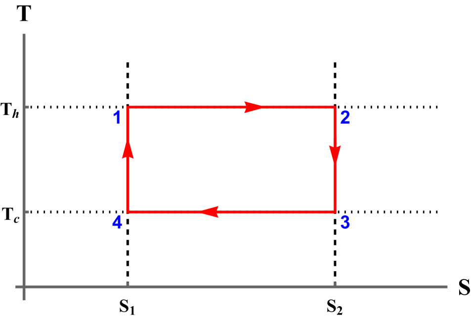
(a) Carnot engine

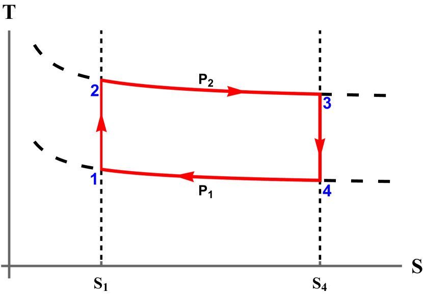
(b) Brayton engine

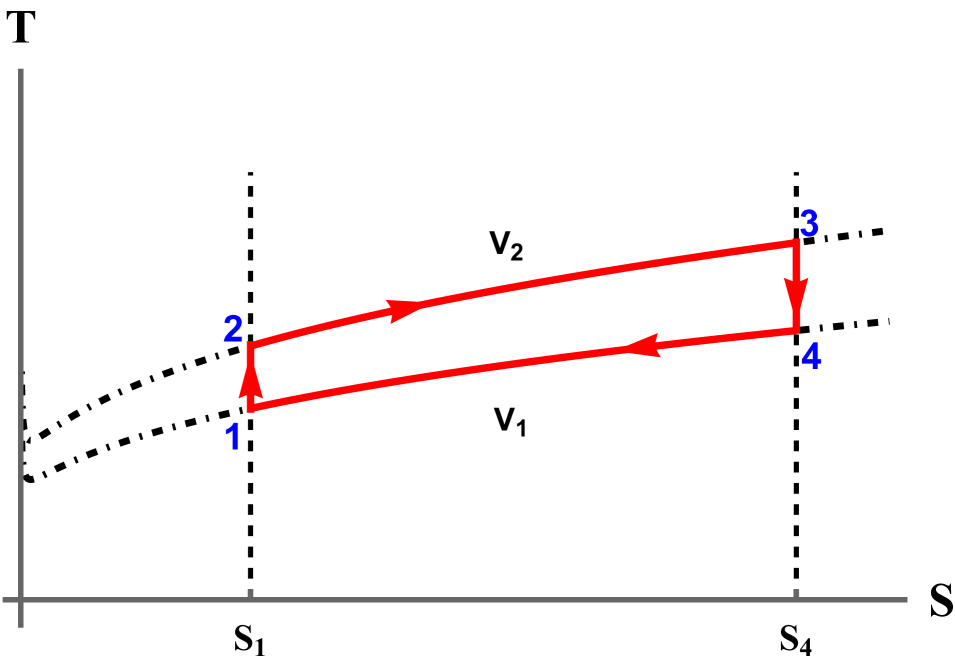
(c) Otto engine

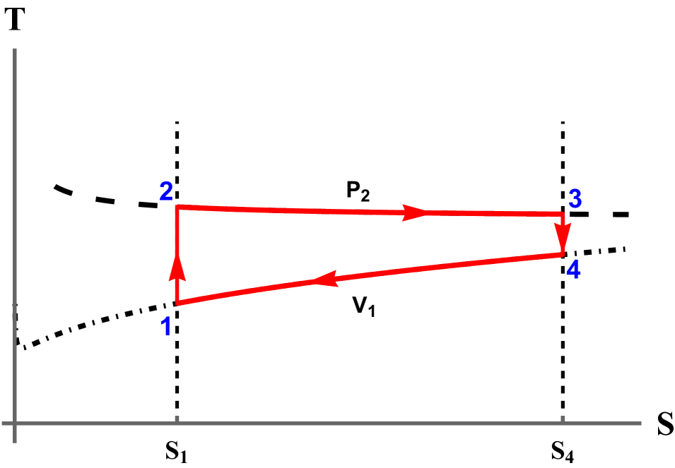
(d) Diesel engine

(e) Rectangle engine

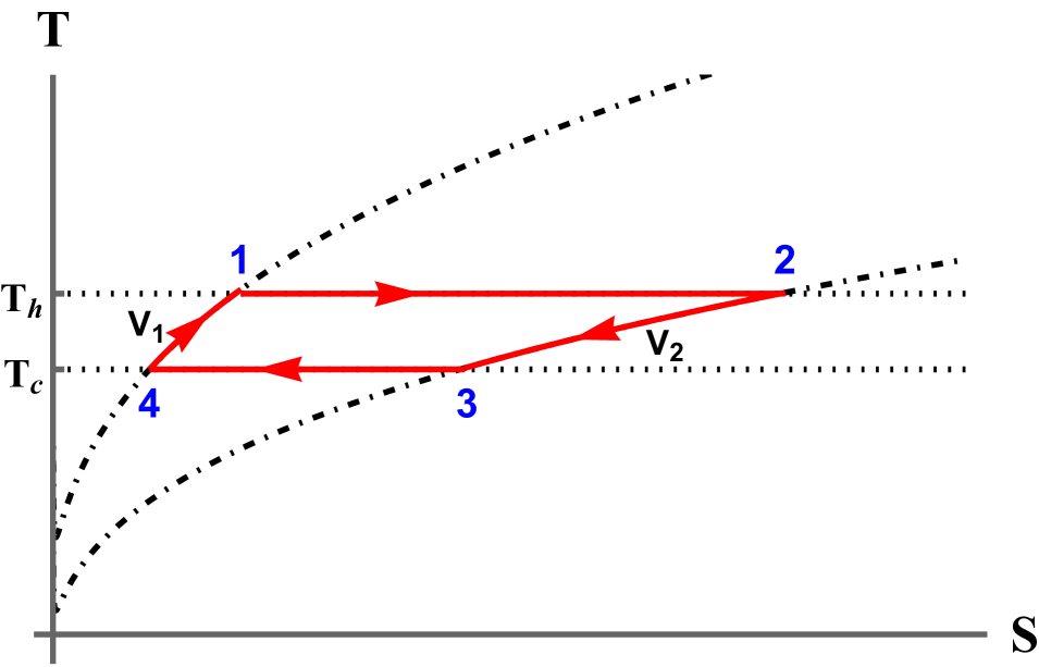
(f) Stirling engine

Figure 5: $TS$-diagrams of Carnot, Brayton, Otto, Diesel, and Stirling engines with a holographic CFT working substance dual to an AdS-Schwarzschild black hole. The plots are for $D=4$ CFT spacetime dimensions. Notably, by comparing the cycles in Figs. 5 and 6 we see that the isochoric and isobaric paths in a $TS$-diagram are different for CFT and ideal gas systems.

Efficiencies of CFT heat engines. We now summarize our results for the efficiencies of various CFT heat engines. The Supplemental Material contains more detailed derivations. We express the efficiencies in terms of the characteristic thermodynamic variables of the engines that are kept fixed along the thermodynamic cycles. For the ideal gas our expressions for the efficiencies are consistent with the literature, e.g., [44, 45, 46, 47, 4]. We plotted the $PV$-diagrams for all heat engines in Figures 3 (for a holographic CFT) and 4 (for a monatomic ideal gas) and the $TS$-diagrams in Figures 5 (for a holographic CFT) and 6 (for a monatomic ideal gas).

A Carnot cycle consists of isothermal expansion ($1\to 2$), adiabatic expansion ($2\to 3$), isothermal compression ($3\to 4$) and adiabatic compression ($4\to 1$). There is an inward heat flow from the hot reservoir to the system along path $1\rightarrow 2$ and an outward heat flow to the cold sink along $3\rightarrow 4$. The Carnot efficiency is

$$\eta_{{\text{Carnot}}}=1-\frac{T_{c}}{T_{h}}\,.$$ (6)

In the Brayton (or Joule) cycle the working substance is first compressed adiabatically ($1\to 2$), heated up isobarically $(2\to 3)$, expanded adiabatically $(3\to 4)$ and cooled isobarically $(4\to 1)$. The Brayton efficiency is

$$\eta_{\text{Brayton}}=1-\left(\frac{P_{1}}{P_{2}}\right)^{\frac{1}{1+\alpha}}\,.$$ (7)

In an Otto cycle, which is a rough approximation of a gasoline engine, the working substance is first compressed adiabatically ($1\rightarrow 2$), then heated up isochorically ($2\rightarrow 3$), expanded adiabatically ($3\rightarrow 4$), and finally cooled isochorically ($4\rightarrow 1$). The Otto efficiency is

$$\eta_{\text{Otto}}=1-\left(\frac{V_{2}}{V_{1}}\right)^{\frac{1}{\alpha}}\,.$$ (8)

The Diesel cycle consists of adiabatic compression $(1\to 2)$, isobaric heating up $(2\to 3)$, adiabatic expansion $(3\to 4)$ and then isochoric cooling ($4\to 1$). In terms of the compression ratio $V_{1}/V_{2}$ and cutoff ratio $V_{3}/V_{2}$ the Diesel efficiency reads

$$\eta_{\text{Diesel}}=1-\frac{\alpha}{\alpha+1}\left(\frac{V_{2}}{V_{1}}\right)^{\frac{1}{\alpha}}\frac{\left(\frac{V_{3}}{V_{2}}\right)^{\frac{\alpha+1}{\alpha}}-1}{\left(\frac{V_{3}}{V_{2}}\right)-1}\,.$$ (9)

The efficiency of the Diesel cycle is always less than that of the Otto cycle if $V_{3}>V_{2}$, for a given compression ratio (see also Figure 1).

For the cycle that forms a rectangle in a $PV$-diagram, paths $2\rightarrow 3$ and $4\rightarrow 1$ are isobars, and paths $1\rightarrow 2$ and $3\rightarrow 4$ are isochores. The efficiency for this cycle is

$$\eta_{\text{rectangular}}=\frac{1}{(\alpha+1)\left(\frac{P_{2}}{P_{2}-P_{1}}\right)+\alpha\left(\frac{V_{1}}{V_{4}-V_{1}}\right)}\,.$$ (10)

Note that for $\gamma>\frac{D}{D-1}$ the Brayton, Otto and rectangular engines are more efficient for ideal gases than for CFT working substances (see Figure 1 for the Otto engine).

The Stirling cycle consists of two isothermal paths (expansion along $1\to 2$ and compression along $3\to 4$), and two isochores ($2\to 3$ and $4\to 1$). In the absence of a regenerative heat exchanger there is heat gain along paths $1\rightarrow 2$ and $4\rightarrow 1$, and heat rejection along the paths $2\rightarrow 3$ and $3\rightarrow 4$. Without regeneration the Stirling efficiency for an ideal gas and generic CFT is

$$\eta_{\text{Stirling}}=1-\frac{T_{c}(S_{3}-S_{4})+\alpha V_{2}(P_{2}-P_{3})}{T_{h}(S_{2}-S_{1})+\alpha V_{1}(P_{1}-P_{4})}\,.$$ (11)

We want to express the efficiency in terms of the $T$ and $V$ alone, which are the characteristic parameters of the Stirling engine, since they are constant along the isotherms and isochores, respectively, and they are experimentally controllable. In order to so do we need to know the functions $S(T,V)$ and $P(T,V)$, which depend on the details of the CFT and the spatial geometry. For concreteness, we now consider a CFT working substance with a characteristic scale $R$ and volume $V\propto R^{D-1}$, such as a round sphere of radius $R$. The dimensionless products $ER$ and $TR$ are then scale invariant, which do not change as one varies the volume. This implies the entropy and dimensionless energy $ER$ only depend on $T$ and $V$ via the product $TR.$ In a high-temperature or large-volume expansion of the entropy and energy the leading term is extensive, i.e., $S\propto(TR)^{D-1}\propto T^{D-1}V$ and $ER\propto(TR)^{D}$, or, equivalently, $E\propto T^{D}V$ [48]. The pressure follows from inserting the scaling of the energy into the conformal equation of state, yielding $P\propto T^{D}$. Moreover, the scaling of the subleading terms in an expansion around $TR=\infty$ is also fixed: the next order is always subleading in $(TR)^{-2}$ with respect to the previous order. For instance, the expansion of the scale invariant product of the canonical free energy $F$ and $R$ in any CFT is [49]

$$-FR=a_{D}(2\pi TR)^{D}+a_{D-2}(2\pi TR)^{D-2}+\mathcal{O}((TR)^{D-4})\,.$$ (12)

From this expansion the entropy and pressure can be explicitly computed via the standard thermodynamic relations $S=-(\partial F/\partial T)_{V}$ and $P=-(\partial F/\partial V)_{T}$. Inserting this into the Stirling efficiency (11) yields

$$\eta_{\text{Stirling}}^{\text{CFT}}=1-\frac{T_{c}^{D}(V_{2}\xi_{12}-V_{1}\xi_{11})+V_{2}\frac{D-1}{D}(T_{h}^{D}\chi_{22}-T_{c}^{D}\chi_{12})}{T_{h}^{D}(V_{2}\xi_{22}-V_{1}\xi_{21})+V_{1}\frac{D-1}{D}(T_{h}^{D}\chi_{21}-T_{c}^{D}\chi_{11})},$$ (13)

where $\xi_{ij}$ and $\chi_{ij}$ are up to order $\mathcal{O}(T_{i}^{-4}V_{j}^{-4/(D-1)})$

$$\xi_{ij} \approx 1+\frac{a_{D-2}(D-2)}{a_{D}D(2\pi)^{2}T_{i}^{2}}\left(\frac{\Omega_{D-1}}{V_{j}}\right)^{\frac{2}{D-1}}\,,$$ (14)

$$\chi_{ij} \approx 1+\frac{a_{D-2}(D-3)}{a_{D}(D-1)(2\pi)^{2}T_{i}^{2}}\left(\frac{\Omega_{D-1}}{V_{j}}\right)^{\frac{2}{D-1}}\,.$$ (15)

Here $T_{1}\equiv T_{c}$ and $T_{2}\equiv T_{h}$. Note the Stirling efficiency is uniquely fixed to leading order in the high-temperature or large-volume expansion. But to subleading order $\eta_{\text{Stirling}}^{\text{CFT}}$ depends on $a_{D}$ and $a_{D-2}$, which are defined via (12) as the coefficients of the leading and subleading terms in the free energy expansion. These coefficients are independent of $(T,V)$, but do depend on the matter content of CFTs. They have been explicitly computed for free CFTs in $D=4$ and $D=6$ in [49]. For instance, for $\mathcal{N}=4$ SYM theory with $SU(N)$ gauge group in $D=4$ we have $a_{4}=(N^{2}-1)/48$ and $a_{2}=-(N^{2}-1)/8$, so $a_{4}/a_{2}=-1/6$.

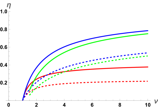
Figure 1: Efficiency $\eta$ vs. compression ratio $v$ (the ratio of larger volume and smaller volume, i.e., $V_{1}/V_{2}$ for Otto and Diesel and $V_{2}/V_{1}$ for Stirling) for Otto (blue), Diesel (green), and Stirling (red) engines in $D=4$. The solid lines correspond to a monatomic ideal gas ($f=3$) and dashed lines to general CFTs (for Stirling: CFT on a plane). The fixed temperature ratio for Stirling is $t\equiv T_{h}/T_{c}=2$ and the fixed cutoff ratio for Diesel is $V_{3}/V_{2}=1.5$. The Otto and Diesel efficiencies asymptote to 1, and the $v\to\infty$ limit of the Stirling efficiency is $1-t^{-1}$ for an ideal gas and $(1-t^{-D})/D$ for a CFT on a plane.

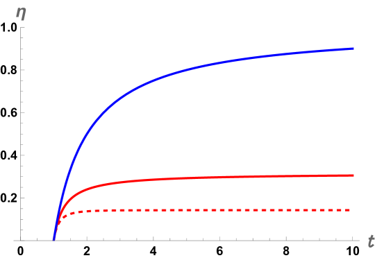
Figure 2: Efficiency $\eta$ vs. temperature ratio $t\equiv T_{h}/T_{c}$ for Stirling (red) and Carnot (blue) engines in $D=4$. The solid lines correspond to a monatomic ideal gas ($f=3$) and the dashed line to a CFT on a plane. The fixed compresion ratio for Stirling is $v\equiv V_{2}/V_{1}=2$. The Carnot efficiency asymptotes to 1, and the Stirling efficiency asymptotes to $(v-1)/(Dv-1)$ for a CFT on a plane and to $\ln(v)/(f/2+\ln(v))$ for an ideal gas.

Further, for an ideal gas the change in the entropy along an isotherm is given as $\Delta S=N\ln\left(V_{2}/V_{1}\right)$ and the pressure is related to the temperature and volume by the equation of state $P=NT/V$. Hence, the Stirling efficiency for an ideal gas is given by

$$\eta_{\text{Stirling}}^{\text{ideal gas}}=1-\frac{T_{c}\ln(V_{2}/V_{1})+\frac{f}{2}(T_{h}-T_{c})}{T_{h}\ln(V_{2}/V_{1})+\frac{f}{2}(T_{h}-T_{c})}\,.$$ (16)

We thus find that the dependence of the Stirling efficiency on $T$ and $V$ is different for an ideal gas and a CFT working substance. In Figure 1 we plotted the efficiency as a function of the compression ratio (at fixed temperature ratio and cutoff ratio) for the Otto, Diesel and Stirling engines, and in Figure 2 we plotted the efficiency as a function of the temperature ratio (at fixed compression ratio) for the Carnot and Stirling engines. These plots show that the efficiency is universally higher for (monatomic) ideal gases than for CFTs.

Holographic heat engines. So far we have considered heat engines for generic CFTs. Next, we construct heat engines for holographic CFT states that are dual to AdS black holes. We stress that the generic CFT results for the engine efficiencies above also hold for holographic CFTs, but for the Stirling engine we can compute the efficiency exactly by invoking holography. For heat engines of holographic CFTs the geometry is fixed to be equivalent (up to Weyl rescaling) to the boundary geometry of the dual black hole spacetime. That is because we take the working substance of holographic heat engines to be the entire spatial geometry of the holographic CFT. Furthermore, we only consider black holes with positive heat capacity, since if the heat capacity were negative the cycles in the $PV$-diagrams 3 and 4 would act as refrigerators (and the reverse cycles would be heat engines). Large enough AdS black holes indeed have positive heat capacity and thus their thermodynamic cycles (in the order $1\to 2\to 3\to 4\to 1$) can operate as heat engines.

Concretely, here we consider static, spherically symmetric, uncharged asymptotically AdS black holes, a.k.a. AdS-Schwarzschild black holes, in $D+1$ spacetime dimensions. Hence, in our setup the spatial geometry of the holographic heat engine is a round sphere with radius $R$ and volume $V=\Omega_{D-1}R^{D-1}.$ For these black holes the holographic dictionary reads [40, 41, 42, 43]

$$S =4\pi Cx^{D-1},\qquad C=\frac{\Omega_{D-1}L^{D-1}}{16\pi G}\,,$$ (17)

$$E =\frac{(D-1)Cx^{D-2}}{R}\left(1+x^{2}\right)\,,$$ (18)

$$T =\frac{D-2}{4\pi Rx}\left(1+\frac{D}{D-2}x^{2}\right)\,,$$ (19)

$$P =\frac{Cx^{D-2}}{\Omega_{D-1}R^{D}}\left(1+x^{2}\right)\,.$$ (20)

We defined $x\equiv r_{h}/L$ with $r_{h}$ the horizon radius of the black hole and $L$ the AdS curvature radius. The heat capacity at fixed $V$ and $C$ is positive if $x>\sqrt{(D-2)/D}$. Crucially, the boundary volume $V$ and the central charge $C$ can be independently varied, since they depend on $R$ and $L$, respectively. In previous dictionaries, e.g., in [50, 51, 40], $R$ was set equal to $L$, so that $V$ and $C$ could be independently varied only if Newton’s constant $G$ is allowed to change. For holographic heat engines, however, we want to keep the theory parameters in the bulk and boundary fixed ($G$ and $C$) while allowing $V$ to vary, which is possible only if $R\neq L$ [42].

We now compute the Stirling efficiency by invoking the holographic dictionary above. From (17)-(20) one can derive exact expressions for $S(T,V)$ and $P(T,V)$ (see Supplemental Material). Inserting them into (11) yields that the Stirling efficiency for CFT states dual to AdS-Schwarzschild takes the same form as (13), but now the functions $\xi_{ij}$ and $\chi_{ij}$ are given by

$$\xi_{ij}=\frac{1}{2^{D-1}}\!\left[1+\sqrt{1-\frac{D(D-2)}{4\pi^{2}T_{i}^{2}}\left(\frac{\Omega_{D-1}}{V_{j}}\right)^{\frac{2}{D-1}}}\right]^{D-1}\,\!\!\!\!\!\!\!\!\!\!,$$ (21)

$$\chi_{ij}=\xi_{ij}^{\frac{D-2}{D-1}}\left[\xi_{ij}^{\frac{2}{D-1}}+\frac{D^{2}}{16\pi^{2}T_{i}^{2}}\left(\frac{\Omega_{D-1}}{V_{j}}\right)^{\frac{2}{D-1}}\right]\,.$$ (22)

These are exact expressions in the temperature and volume. We can expand them at high temperature or large volume. The result up to subleading order is the same as (14) and (15) with the ratio of the coefficients given by

$$\frac{a_{D-2}}{a_{D}}=-\frac{D^{2}(D-1)}{4}\,.$$ (23)

This agrees with earlier findings for these coefficients in holographic CFTs [48, 49]. Interestingly, the holographic Stirling efficiency is lower than the leading order contribution to the efficiency in the high-temperature and large-volume expansion, for which $\xi_{ij}=\chi_{ij}=1$. Moreover, we checked by plotting that for $\mathcal{N}=4$ SYM theory in $D=4$ the Stirling efficiency is higher at zero ’t Hooft coupling (for which $a_{4}/a_{2}=-1/6$) than at infinite coupling (with $a_{4}/a_{2}=-1/12$, cf. (23)). Thus, this suggests for CFTs the Stirling efficiency decreases as the coupling increases.

Discussion. In this paper we proposed a novel way to construct heat engines in holographic field theories. The working substance can be modeled by a strongly coupled, large-$N$ thermal system that is dual to a black hole spacetime [16, 52]. A crucial aspect of the holographic dictionary that we used is that the volume can be independently varied from the other thermodynamic variables. We computed the efficiencies of various idealized engines for (holographic) CFTs.

For future work there are many generalizations of our setup worth studying. We only described the simplest holographic heat engines as a proof of principle that our construction works. First, one could study other types of engines, ideally more realistic ones for which the efficiency of holographic systems can be experimentally tested. Second, we considered only field theories with conformal symmetry, but one could define heat engines for holographic field theories with different global symmetries, such as anisotropic scaling symmetry [53, 54]. Third, one could compute the Stirling efficiency for specific CFTs at finite temperature and volume, for instance perturbatively at weak coupling, and compare with the holographic result. Finally, one could study holographic engines for different types of black holes, such as charged or rotating black holes or black hole solutions to higher curvature gravity.

Acknowledgments: MV is grateful to S. Borsboom, K. Landsman, J. Uffink, and E. Verlinde for discussions on related topics. This work is supported in part by the Spinoza Grant of the Dutch Science Organization (NWO) awarded to Klaas Landsman.

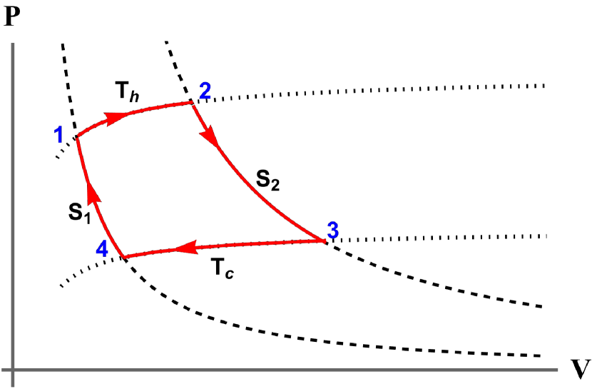
(a) Carnot engine

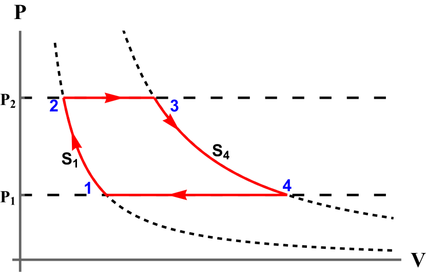
(b) Brayton engine

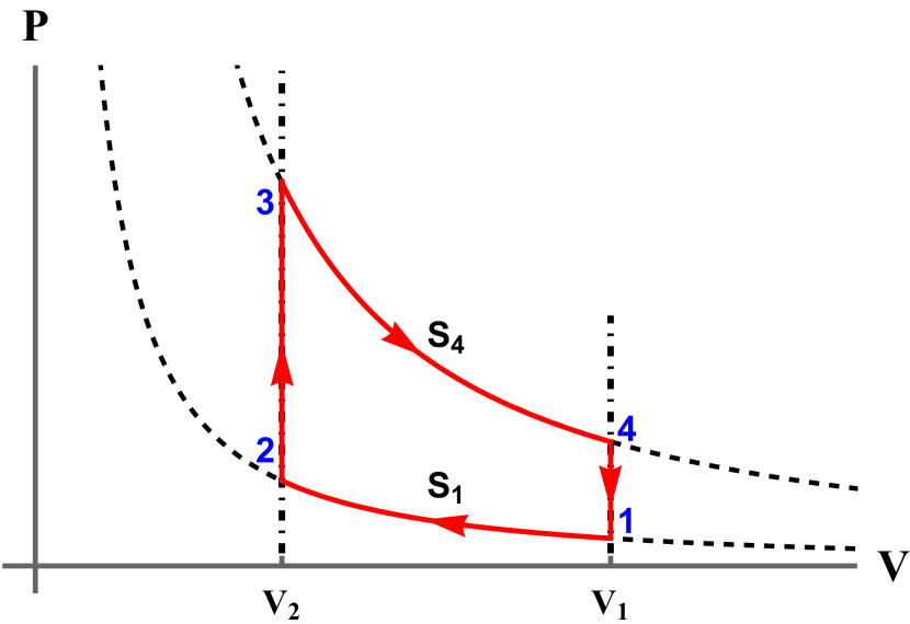
(c) Otto engine

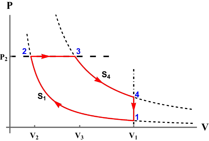
(d) Diesel engine

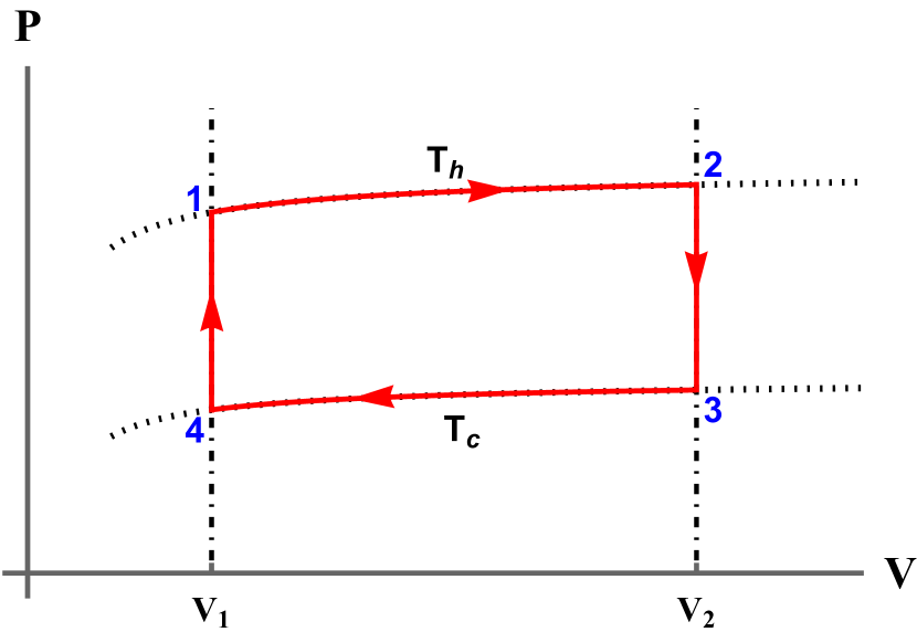
(e) Stirling engine

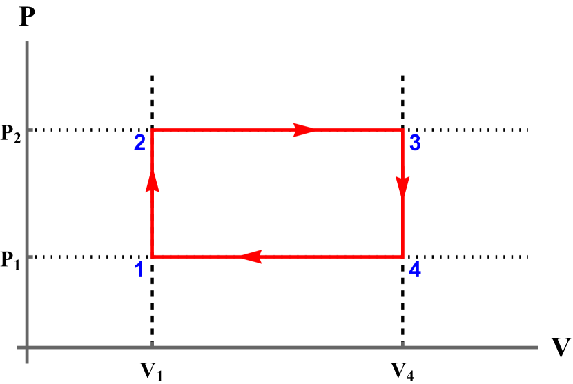
(f) Rectangle engine

Figure 3: $PV$-diagrams of Carnot, Brayton, Otto, Diesel, and Stirling cycles for a thermal CFT system dual to an AdS-Schwarzschild black hole. The plots are for $D=4$ CFT spacetime dimensions. In all figures in this article dotted lines correspond to isotherms, short dashed lines to adiabats, long dashed lines to isobars, and dotdashed lines to isochores. Further, $T_{h}$ is the temperature of the heat source, and $T_{c}$ the temperature of the heat sink. Notably, by comparing the Carnot (Figs. 3a and 4a) and Stirling cycles (Figs. 3e and 4b) we see that the isotherm for a CFT monotonically increases with $V$ whereas the isotherm for the ideal gas monotonically decreases with $V$. The slope of the adiabats is also different for the two systems. In the Supplemental Material we derive the equations for the various paths that are used to make these plots.

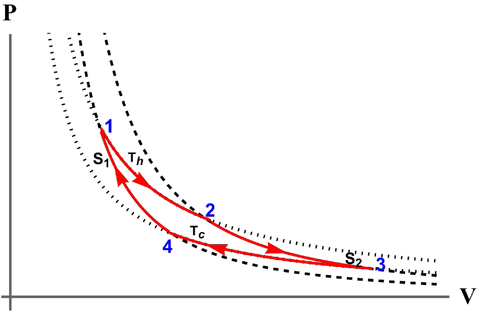
(a) Carnot engine

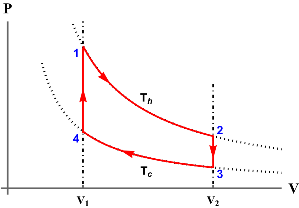
(b) Stirling engine

Figure 4: $PV$-diagrams of Carnot and Stirling engines with a monatomic ($\gamma=5/3$) ideal gas in $D=4$ as the working substance. The $PV$-diagrams for the CFT and ideal gas systems are identical for the Brayton, Otto, Diesel and rectangle engines, but different for the Carnot and Stirling engine.

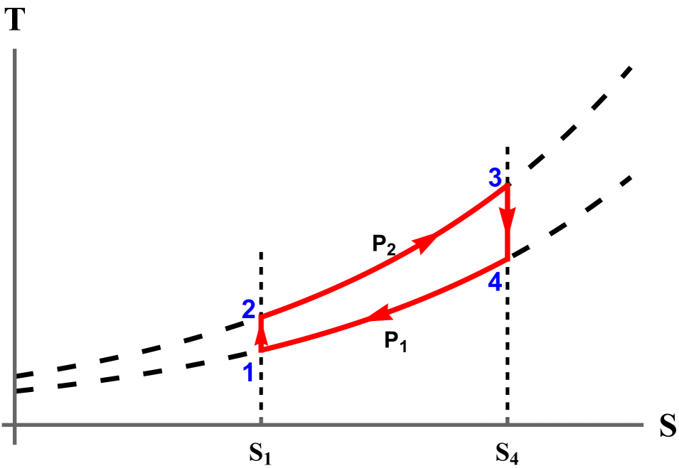
(a) Brayton engine

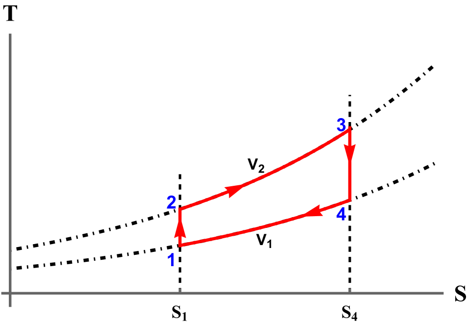
(b) Otto engine

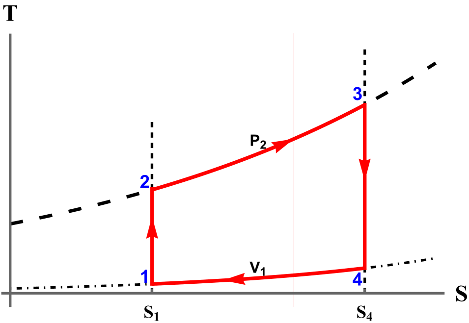
(c) Diesel engine

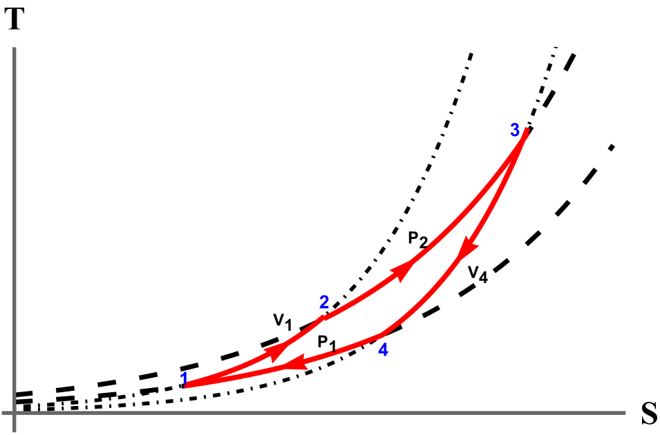
(d) Rectangle engine

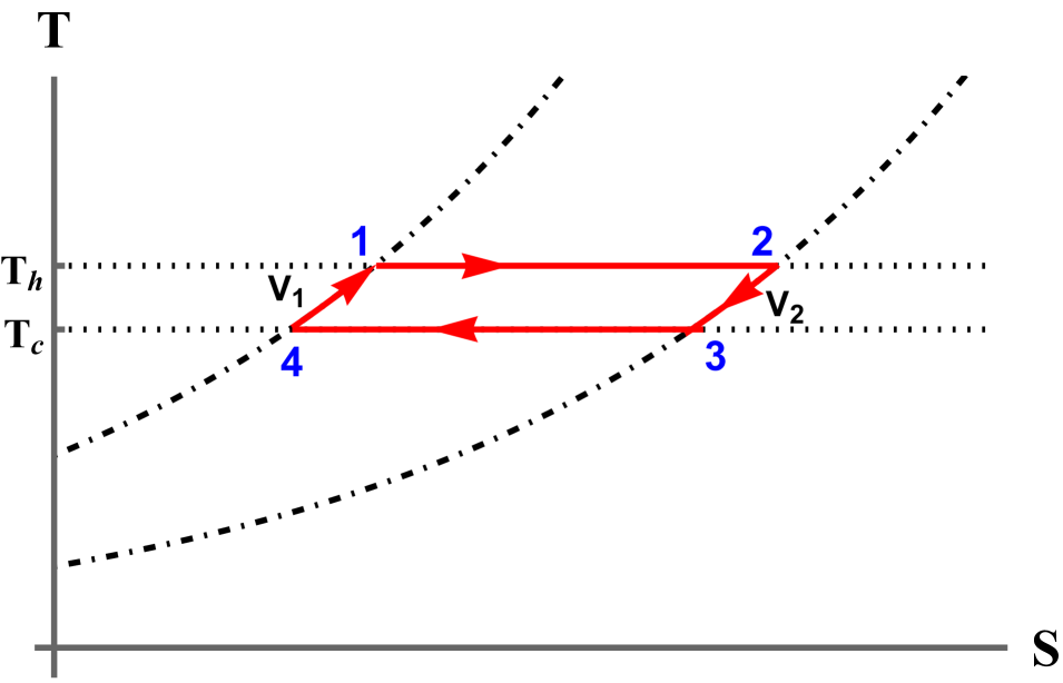
(d) Stirling engine

Figure 6: $TS$-diagrams of Brayton, Otto, Diesel, and Stirling engines with monatomic ($\gamma=5/3$) ideal gas in $D=4$ as the working substance. The $TS$-plots corresponding to the CFT and ideal gase systems are different for these engines, but identical for the Carnot engine.

Supplemental Material

Appendix A Efficiencies of CFT and ideal gas heat engines

In this appendix we compute the efficiencies of various heat engines for CFT and ideal gas working substances. We recall that both thermal systems satisfy the equation of state $E=\alpha PV$, where $\alpha=D-1$ for CFTs and $\alpha=f/2=1/(\gamma-1)$ for an ideal gas with $f$ number of degrees of freedom (and $\gamma\equiv C_{P}/C_{V}$). Regarding sign conventions, we take the following three quantities all to be positive: heat input $Q_{\text{in}}$ from the heat source into the system, the heat output $Q_{\text{out}}$ from the system to the heat sink and the work $W$ produced in the engine, that is done by the system on the work source. Note this is different from the sign convention in the first law, $\Delta E=Q-W$, where $Q$ is positive when it is added to the system and negative when it leaves. So with a subscript $Q_{\text{in/out}}$ is always positive and without a subscript $Q$ can be negative.

Carnot engine. In a Carnot cycle the heat exchange takes place only along the two isotherms (because $Q=0$ along the adiabats) with an inward heat flow along $1\rightarrow 2$ and an outward flow along the path $3\rightarrow 4$. From the Clausius relation (3) it follows that $Q_{\text{in}}=Q_{\text{in}}^{1\rightarrow 2}=T_{h}(S_{2}-S_{1})$ and $Q_{\text{out}}=Q_{\text{out}}^{3\rightarrow 4}=T_{c}(S_{3}-S_{4})=T_{c}(S_{2}-S_{1})$, since along the adiabats $2\to 3$ and $4\to 1$ we have $S_{2}=S_{3}$ and $S_{1}=S_{4}$, respectively. Thus, the efficiency of a Carnot engine is

$$\eta_{{\text{Carnot}}}=1-\frac{Q_{\text{out}}^{3\rightarrow 4}}{Q_{\text{in}}^{1\rightarrow 2}}=1-\frac{T_{c}}{T_{h}}\,,$$ (24)

which is indeed the Carnot efficiency. Note that we did not use an equation of state to derive this efficiency, so it holds for any working substance.

Brayton engine. In the Brayton (or Joule) cycle there is heat exchange along the two isobaric paths, with an inward flow along the path $2\rightarrow 3$ and an outward flow along $4\rightarrow 1$. There is no heat exchange along the adiabatic paths $1\rightarrow 2$ and $3\rightarrow 4$. From the first law it follows that the heat exchange along an isobar is equal to the change in enthalpy: $Q=\Delta E+P\Delta V=\Delta(E+PV)\equiv\Delta H$. For a CFT and ideal gas the enthalpy is $H=(\alpha+1)PV$. Hence $Q_{\text{in}}=Q_{\text{in}}^{2\rightarrow 3}=H_{3}-H_{2}=(\alpha+1)P_{2}(V_{3}-V_{2})$ and $Q_{\text{out}}=Q_{\text{out}}^{4\rightarrow 1}=-(H_{1}-H_{4})=(\alpha+1)P_{1}(V_{4}-V_{1})$. The adiabat relation (5) for the paths $1\to 2$ and $3\to 4$ yields

$$P_{2}V_{2}^{\frac{\alpha+1}{\alpha}}=P_{1}V_{1}^{\frac{\alpha+1}{\alpha}}\,,\qquad P_{2}V_{3}^{\frac{\alpha+1}{\alpha}}=P_{1}V_{4}^{\frac{\alpha+1}{\alpha}}\,.$$ (25)

Dividing these two equations implies the volume ratios are equal: $V_{2}/V_{3}=V_{1}/V_{4}$. From this equality and (25) we obtain the efficiency for the Brayton engine

$$\eta_{\text{Brayton}}=1-\frac{Q_{\text{out}}^{4\rightarrow 1}}{Q_{\text{in}}^{2\rightarrow 3}}=1-\frac{H_{4}-H_{1}}{H_{3}-H_{2}}=1-\left(\frac{P_{1}}{P_{2}}\right)^{\frac{1}{1+\alpha}}\,.$$ (26)

The Brayton efficiency for a CFT working substance thus depends on the number of dimensions. Note that for $\gamma>\frac{D}{D-1}$ the ideal gas Brayton engine is more efficient than the corresponding CFT engine. For instance, a Brayton engine consisting of a monatomic gas ($f=D-1,\gamma=(D+1)/(D-1)$) or diatomic gas ($f=2D-3,\gamma=(2D-1)/(2D-3)$) is more efficient than a CFT Brayton engine in $D$ spacetime dimensions.

Otto engine. In an Otto cycle the processes along $1\rightarrow 2$ and $3\rightarrow 4$ are adiabatic and the processes along $2\rightarrow 3$ and $4\rightarrow 1$ are isochoric (which implies $V_{1}=V_{4}$ and $V_{2}=V_{3})$. There is heat loss along $4\rightarrow 1$ and heat gain along $2\rightarrow 3$. From the first law it follows that heat exchange along isochores is equal to the change in internal energy. Thus, $Q_{\text{in}}=Q_{\text{in}}^{2\rightarrow 3}=E_{3}-E_{2}=\alpha V_{2}(P_{3}-P_{2})$ and $Q_{\text{out}}=Q_{\text{out}}^{4\rightarrow 1}=-(E_{1}-E_{4})=\alpha V_{1}(P_{4}-P_{1})$. The relation for the two adiabats $1\to 2$ and $3\to 4$ is

$$P_{2}V_{2}^{\frac{\alpha+1}{\alpha}}=P_{1}V_{1}^{\frac{\alpha+1}{\alpha}}\,,\qquad P_{3}V_{2}^{\frac{\alpha+1}{\alpha}}=P_{4}V_{1}^{\frac{\alpha+1}{\alpha}}\,.$$ (27)

Dividing these two equations yields that the pressure ratios are equal: $P_{3}/P_{2}=P_{4}/P_{1}$. Using this equality and (27) we find the Otto efficiency

$$\eta_{\text{Otto}}=1-\frac{Q_{\text{out}}^{4\rightarrow 1}}{Q_{\text{in}}^{2\rightarrow 3}}=1-\frac{E_{4}-E_{1}}{E_{3}-E_{2}}=1-\left(\frac{V_{2}}{V_{1}}\right)^{\frac{1}{\alpha}}\,.$$ (28)

Diesel engine. In the Diesel cycle paths $1\rightarrow 2$ and $3\rightarrow 4$ are adiabats, path $2\rightarrow 3$ is an isobar (which implies $P_{2}=P_{3}$), and path $4\rightarrow 1$ is an isochore (which implies $V_{4}=V_{1}$). There is heat gain along $2\rightarrow 3$ and heat loss along $4\rightarrow 1$. For the isobar we use that the heat exchange is equal to the change in enthalpy, and for the isochore the heat exchange is equal to the change in internal energy. Thus, $Q_{\text{in}}=Q_{\text{in}}^{2\rightarrow 3}=H_{3}-H_{2}=(\alpha+1)P_{2}(V_{3}-V_{2})$ and $Q_{\text{out}}=Q_{\text{out}}^{4\rightarrow 1}=-(E_{1}-E_{4})=\alpha V_{1}(P_{4}-P_{1})$. Moreover, the two adiabats $1\rightarrow 2$ and $3\rightarrow 4$ satisfy the relations

$$P_{1}V_{1}^{\frac{\alpha+1}{\alpha}}\,=P_{2}V_{2}^{\frac{\alpha+1}{\alpha}},\qquad P_{2}V_{3}^{\frac{\alpha+1}{\alpha}}=P_{4}V_{1}^{\frac{\alpha+1}{\alpha}}\,.$$ (29)

Inserting these adiabat relations into the equations for the heat transfers we obtain the Diesel efficiency

$$\eta_{\text{Diesel}}=1-\frac{Q_{\text{out}}^{4\rightarrow 1}}{Q_{\text{in}}^{2\rightarrow 3}}=1-\frac{E_{4}-E_{1}}{H_{3}-H_{2}}=1-\frac{\alpha}{\alpha+1}\left(\frac{V_{2}}{V_{1}}\right)^{\frac{1}{\alpha}}\frac{\left(\frac{V_{3}}{V_{2}}\right)^{\frac{\alpha+1}{\alpha}}-1}{\left(\frac{V_{3}}{V_{2}}\right)-1}\,.$$ (30)

We checked by plotting in various dimensions that the CFT efficiency is less than the efficiency for a monatomic and diatomic ideal gas.

Rectangle engine. In this cycle paths $2\rightarrow 3$ and $4\rightarrow 1$ are isobars, i.e., $P_{2}=P_{3}$ and $P_{4}=P_{1}$, and paths $1\rightarrow 2$ and $3\rightarrow 4$ are isochores, i.e., $V_{1}=V_{2}$ and $V_{3}=V_{4}$. There is an inward flow of heat along $1\rightarrow 2$ and $2\rightarrow 3$, whereas there is an outward flow of heat along the paths $3\to 4$ and $4\to 1$. Along the isobars the heat input is equal to the enthalpy difference, and along the isochores the heat change is equal to the internal energy difference. Thus, the total heat that flows into the system is given by

$$Q_{\text{in}}=Q_{\text{in}}^{1\rightarrow 2}+Q_{\text{in}}^{2\rightarrow 3}=(E_{2}-E_{1})+(H_{3}-H_{2})=\alpha V_{1}(P_{2}-P_{1})+(\alpha+1)P_{2}(V_{4}-V_{1})\,.$$ (31)

For this engine the work produced can be easily calculated, since it is the area enclosed by the cycle

$$W=(P_{2}-P_{1})(V_{4}-V_{1})\,.$$ (32)

Thus, substituting for enthalpy and internal energy in (31), we get the following efficiency

$$\eta_{\text{rectangular}}=\frac{W}{Q_{\text{in}}}=\frac{1}{(\alpha+1)\left(\frac{P_{2}}{P_{2}-P_{1}}\right)+\alpha\left(\frac{V_{1}}{V_{4}-V_{1}}\right)}\,.$$ (33)

The CFT engine is less efficient than the corresponding ideal gas engine if $\gamma>\frac{D}{D-1}$.

Stirling engine. In a Stirling cycle paths $1\rightarrow 2$ and $3\rightarrow 4$ are isotherms and paths $2\rightarrow 3$ and $4\rightarrow 1$ are isochores (hence $V_{2}=V_{3}$ and $V_{4}=V_{1}$). In the absence of a regenerator, there is heat gain along paths $1\rightarrow 2$ and $4\rightarrow 1$, and there is heat loss along the paths $2\rightarrow 3$ and $3\rightarrow 4$. The heat transfer along the isochores is equal to the change in internal energy, and the heat exchange along the isotherm follows from the Clausius relation (3). Thus, $Q_{\text{in}}=Q_{\text{in}}^{1\rightarrow 2}+Q_{\text{in}}^{4\rightarrow 1}=T_{h}(S_{2}-S_{1})+\alpha V_{1}(P_{1}-P_{4})$ and $Q_{\text{out}}=Q_{\text{out}}^{2\rightarrow 3}+Q_{\text{out}}^{3\rightarrow 4}=-\alpha V_{2}(P_{3}-P_{2})-T_{c}(S_{4}-S_{3})$. Hence, the Stirling efficiency can be written as follows

$$\eta_{\text{Stirling}}=1-\frac{Q_{\text{out}}^{2\to 3}+Q_{\text{out}}^{3\to 4}}{Q_{\text{in}}^{1\to 2}+Q_{\text{in}}^{4\to 1}}=1-\frac{T_{c}(S_{3}-S_{4})+\alpha V_{2}(P_{2}-P_{3})}{T_{h}(S_{2}-S_{1})+\alpha V_{1}(P_{1}-P_{4})}\,.$$ (34)

Appendix B Equations for thermodynamic processes in the $PV$- and $TS$-cycles

In this appendix we explain how the $PV$- and $TS$-diagrams in Figures 3 to 6 are obtained for the CFT dual to the AdS-Schwarzschild black hole and the ideal gas. To construct the $PV$ cycles for various engines, it is necessary to determine the equations of the various paths, namely the adiabat, isotherm, isochore, and isobar. In the $P-V$ plane, the equations for an isobar and isochore are simply $P=\text{const}.$ and $V=\text{const}.$, respectively. Further, the equation for an adiabat in a CFT is given by

$$PV^{\frac{D}{D-1}}=\text{constant}\qquad\text{(adiabat for CFT)}\,.$$ (35)

This adiabat relation can be derived from the first law (2) and the equation of state (4). Both volume and pressure vary along the adiabat, hence the equation of state yields $\Delta E=\alpha(P\Delta V+V\Delta P)$. Since there is no heat exchange along an adiabat ($Q=0$), it follows from the first law that, $(\alpha+1)P\Delta V+\alpha V\Delta P=0.$ Dividing both sides by $\alpha PV$ and integrating we arrive at (5). Finally, inserting $\alpha=D-1$ for a CFT into (5) yields (35).

To determine the equation of the isotherm for the holographic CFT engine, we first solve for $x$ in terms of $T$ and $V$ from (19), see equation (70), and substitute $x(T,V)$ in the expression for pressure $P(V,C,x)$ (20). Further, since temperature is constant along an isotherm, we fix the temperature to $T_{o}$ (and we also fix the central charge $C$). We arrive at the following equation for the isotherm

$$PV^{\frac{D}{D-1}}=C(\Omega_{D-1})^{\frac{1}{D-1}}\left[\frac{1}{D}\left(2\pi T_{o}\left(\frac{V}{\Omega_{D-1}}\right)^{\frac{1}{D-1}}+\sqrt{4\pi^{2}T_{o}^{2}\left(\frac{V}{\Omega_{D-1}}\right)^{\frac{2}{D-1}}-D(D-2)}\right)\right]^{D-2}\times$$ (36)

$$\quad\times\left[1+\left(\frac{1}{D}\left(2\pi T_{o}\left(\frac{V}{\Omega_{D-1}}\right)^{\frac{1}{D-1}}+\sqrt{4\pi^{2}T_{0}^{2}\left(\frac{V}{\Omega_{D-1}}\right)^{\frac{2}{D-1}}-D(D-2)}\right)\right)^{2}\right]\qquad\text{(isotherm for holographic CFT)}\,.$$

With the equations for all the thermodynamic processes at hand, we can obtain the $PV$-plots for all the holographic heat engines in Appendix A.

For an ideal gas the equation for an adiabat is

$$PV^{\gamma}=\text{constant}\qquad\text{(adiabat for ideal gas)}\,.$$ (37)

Moreover, the equation of the isotherm for an ideal gas is given by its equation of state

$$PV=NT_{o}\qquad\text{(isotherm for ideal gas)}\,.$$ (38)

We also derive an equation for $\Delta S$ for an ideal gas along an isotherm, since we use that in the main text in computing the Stirling efficiency. We first note that the change in the internal energy of an ideal gas along an isotherm is zero, due to equipartition $E=\frac{f}{2}NT$ (if we fix $N$). Hence, the first law implies $Q=P\Delta V$ along an isotherm. Substituting the Clausius relation $Q=T\Delta S$ and the equation of state $P=NT/V$ in the first law and integrating on both sides, yields $\Delta S=N\log(V_{2}/V_{1}).$

Next, we determine the equations for various paths in the $TS$-diagrams. In the $T-S$ plane, the equations for adiabats and isotherms are simply $T=\text{const}.$ and $S=\text{const}.$, respectively. To determine the equation for the isochore for thermal CFT systems dual to an AdS-Schwarzschild black hole, we make use of expression (19) for the temperature and substitute $x$ in terms of $S$ from (17) and further fix the volume to $V_{o}$, yielding

$$T=\frac{D-2}{4\pi}\left(\frac{\Omega_{D-1}}{V_{o}}\right)^{\frac{1}{D-1}}\left(\frac{4\pi C}{S}\right)^{\frac{1}{D-1}}\left(1+\frac{D}{D-2}\left(\frac{S}{4\pi C}\right)^{\frac{2}{D-1}}\right)\qquad\text{(isochore for holographic CFT)}\,.$$ (39)

To obtain the equation for an isobar, we first find $V$ in terms of $P$, $S$ and $C$ by combining the expressions (20) and (17) for the pressure $P(V,C,x)$ and $x(S,C)$, respectively, and solving for $V$. Then we substitute $V(P,S,C)$ into (39) and fix the pressure to $P_{o}$. Finally, the isobar equation in the $T-S$ plane becomes

$$T=\frac{D-2}{4\pi}\left(\frac{P_{o}\Omega_{D-1}}{C}\right)^{\frac{1}{D}}\frac{\left[1+\frac{D}{D-2}\left(\frac{S}{4\pi C}\right)^{\frac{2}{D-1}}\right]}{\left[\left(\frac{S}{4\pi C}\right)^{2}\left(1+\left(\frac{S}{4\pi C}\right)^{\frac{2}{D-1}}\right)\right]^{\frac{1}{D}}}\qquad\text{(isobar for holographic CFT)}\,.$$ (40)

The isochore equation for the ideal gas case can be obtained from equation (1a) on page 19 of [55]

$$T=\exp\left[\frac{(\gamma-1)S}{N}-\gamma\right]\left(\frac{V_{o}}{N}\right)^{-(\gamma-1)}\frac{1}{2\pi m}\qquad\text{(isochore for ideal gas)}\,.$$ (41)

where $m$ is the mass of the gas particles. The isobar equation can be obtained by writing $V_{0}$ in terms of $P_{0}$ in (41), using the ideal gas equation of state $V/N=T/P$,

$$T^{\gamma}=\exp\left[\frac{(\gamma-1)S}{N}-\gamma\right]P_{o}^{\gamma-1}\frac{1}{2\pi m}\qquad\text{(isobar for ideal gas)}\,.$$ (42)

These expressions allow us to obtain the $TS$-diagrams for various holographic and ideal gas heat engines.

Appendix C High-temperature expansion of the Stirling efficiency for a CFT on a sphere

Consider a general conformal field theory on a round sphere $S^{D-2}$ at finite temperature. The perturbative expansion of the canonical free energy $F$ around $TR=\infty$ takes the form [49]

$$-FR=a_{D}(2\pi RT)^{D}+a_{D-2}(2\pi RT)^{D-2}+a_{D-4}(2\pi TR)^{D-4}+\cdots\,.$$ (43)

At strong ’t Hooft coupling the high-temperature expansion of the free energy includes an infinite series in $1/(TR)$, whereas at zero coupling the coefficients of all the terms that scale with negative powers of $TR$ are absent. Non-perturbative corrections appear at order $\mathcal{O}(e^{-(2\pi)^{2}TR})$, which we ignore. Below we compute the Stirling efficiency in the high-temperature or large-volume expansion up to subsubleading order, i.e. keeping the coefficients $a_{D},a_{D-2}$ and $a_{D-4}$ finite and neglecting higher-order corrections.

The entropy $S$, energy $E$ and pressure $P$ can be derived from the free energy as follows

$$S =-\left(\frac{\partial F}{\partial T}\right)_{V}=a_{D}D2\pi(2\pi TR)^{D-1}+a_{D-2}(D-2)2\pi(2\pi TR)^{D-3}+a_{D-4}(D-4)2\pi(2\pi RT)^{D-5}+\cdots$$ (44)

$$ER =FR-TR\left(\frac{\partial F}{\partial T}\right)_{V}=a_{D}(D-1)(2\pi TR)^{D}+a_{D-2}(D-3)(2\pi TR)^{D-2}+a_{D-4}(D-5)(2\pi RT)^{D-4}+\cdots$$ (45)

$$P =-\left(\frac{\partial F}{\partial V}\right)_{T}=\frac{1}{(D-1)VR}\left(a_{D}(D-1)(2\pi TR)^{D}+a_{D-2}(D-3)(2\pi TR)^{D-2}+a_{D-4}(D-5)(2\pi TR)^{D-4}+\cdots\right)\,.$$ (46)

Inserting these functions $S(T,V)$ and $P(T,V)$ into the Stirling efficiency (11) yields

$$\eta_{\text{Stirling}}^{\text{CFT}}=1-\frac{T_{c}^{D}(V_{2}\xi_{12}-V_{1}\xi_{11})+V_{2}\frac{D-1}{D}(T_{h}^{D}\chi_{22}-T_{c}^{D}\chi_{12})}{T_{h}^{D}(V_{2}\xi_{22}-V_{1}\xi_{21})+V_{1}\frac{D-1}{D}(T_{h}^{D}\chi_{21}-T_{c}^{D}\chi_{11})},$$ (47)

where $\xi_{ij}$ and $\chi_{ij}$ are up to order $\mathcal{O}(T_{i}^{-6}V_{j}^{-6/(D-1)})$

$$\xi_{ij} =1+\frac{a_{D-2}(D-2)}{a_{D}D(2\pi)^{2}T_{i}^{2}}\left(\frac{\Omega_{D-1}}{V_{j}}\right)^{\frac{2}{D-1}}+\frac{a_{D-4}(D-4)}{a_{D}D(2\pi)^{4}T_{i}^{4}}\left(\frac{\Omega_{D-1}}{V_{j}}\right)^{\frac{4}{D-1}}+\cdots$$ (48)

$$\chi_{ij} =1+\frac{a_{D-2}(D-3)}{a_{D}(D-1)(2\pi)^{2}T_{i}^{2}}\left(\frac{\Omega_{D-1}}{V_{j}}\right)^{\frac{2}{D-1}}+\frac{a_{D-4}(D-5)}{a_{D}(D-1)(2\pi)^{4}T_{i}^{4}}\left(\frac{\Omega_{D-1}}{V_{j}}\right)^{\frac{4}{D-1}}+\cdots$$ (49)

Here $T_{1}\equiv T_{c}$ and $T_{2}\equiv T_{h}$. The subleading corrections to the Stirling efficiency thus depend on the coefficients in the free energy expansion, which are fixed by the matter content of the CFT. For free CFTs in $D=4$ with $n_{S}$ scalars, $n_{F}$ Weyl fermions and $n_{V}$ vector fields the free energy coefficients are given by [49]

$$a_{4} =\frac{1}{720}\left(n_{S}+2n_{V}+\frac{7}{4}n_{F}\right)\,,$$ (50)

$$a_{2} =-\frac{1}{24}\left(2n_{V}+\frac{1}{4}n_{F}\right)\,,$$ (51)

$$a_{0} =\frac{1}{240}\left(n_{S}+22n_{V}+\frac{17}{4}n_{F}\right)\,.$$ (52)

For instance, $\mathcal{N}=4$ SYM theory with $SU(N)$ gauge group has $6n$ scalars, $4n$ Weyl fermions and $n$ gauge bosons, with $n=N^{2}-1$, so these coefficients are in this case: $a_{4}=n/48,a_{2}=-n/8$ and $a_{0}=3n/16$, hence $a_{2}=-6a_{4}$ and $a_{0}=9a_{4}$. Moreover, for $D$-dimensional holographic CFT states dual a $(D+1)$-dimensional AdS-Schwarzschild black hole the coefficients are

$$\frac{a_{D-2}}{a_{D}}=-\frac{D^{2}(D-1)}{4}\qquad\text{and}\qquad\frac{a_{D-4}}{a_{D}}=\frac{D^{3}(D-2)^{2}(D-1)}{32}\,,$$ (53)

since with this choice of coefficients the expressions (48)-(49) match with (76)-(77) below. For instance, in $D=4$ we have $a_{2}=-12a_{4}$, $a_{0}=24a_{4}$. Assuming these formulae are valid at strong coupling in $\mathcal{N}=4$ SYM in $D=4$, the coefficients flow modestly from weak to strong coupling. It is well known that the leading coefficient at strong ’t Hooft coupling $\lambda(\equiv g^{2}N)=\infty$ is $3/4$ times the leading coefficient at weak coupling $\lambda=0$ [56]. This implies for the coupling dependence of the other coefficients:

$$a_{4}(\lambda=\infty)=\frac{3}{4}a_{4}(\lambda=0)\,,\qquad a_{2}(\lambda=\infty)=\frac{3}{2}a_{2}(\lambda=0)\,,\qquad a_{0}(\lambda=\infty)=2a_{0}(\lambda=0)\,.$$ (54)

The second relation was also derived in [49].

Finally, in order to relate the high-temperature expansion in [49] with the large entropy expansion in [48], we express $TR$ and $ER$ as a function of $S$. We first solve (44) for $TR$ and then insert this expression into (45), yielding

$$TR =\frac{1}{(a_{D}D(2\pi)^{D})^{\frac{1}{D-1}}}S^{\frac{1}{D-1}}-\frac{(D-2)a_{D-2}}{(D-1)(a_{D}2\pi D)^{\frac{D-2}{D-1}}}S^{-\frac{1}{D-1}}\,,$$ (55)

$$ER =\frac{D-1}{(a_{D}(2\pi D)^{D})^{\frac{1}{D-1}}}S^{\frac{D}{D-1}}-\frac{a_{D-2}}{(a_{D}2\pi D)^{\frac{D-2}{D-1}}}S^{\frac{D-2}{D-1}}+\cdots\,.$$ (56)

Comparing this to the large entropy expansion in [48]

$$ER=\frac{a}{4\pi}S^{\frac{D}{D-1}}+\frac{b}{4\pi}S^{\frac{D-2}{D-1}}\,,$$ (57)

we can read off the relation between $(a_{D},a_{D-2})$ and $(a,b)$. In particular, the ratio of $a_{D-2}$ and $a_{D}$ is proportional to the product $ab$

$$\frac{a_{D-2}}{a_{D}}=-\frac{abD^{2}}{4(D-1)}\,.$$ (58)

Hence, the holographic result (53) for the free energy coefficients translates into $ab=(D-1)^{2}$, consistent with [48].

Appendix D Holographic dictionary for the thermodynamics of AdS-Schwarzschild black holes

In this appendix we derive the holographic dictionary for the thermodynamic variables of AdS-Schwarzschild black holes, which are solutions to the Einstein equation with a negative cosmological constant. The line element of AdS-Schwarzschild geometry in static coordinates in $D+1$ dimensions is

$$ds^{2}=-f(r)dt^{2}+\frac{dr^{2}}{f(r)}+r^{2}d\Omega_{D-2}^{2}\,,$$ (59)

with blackening factor

$$f(r)=1+\frac{r^{2}}{L^{2}}-\frac{m}{r^{D-2}}\,,\qquad\text{where}\qquad m=r_{h}^{D-2}\left(1+\frac{r_{h}^{2}}{L^{2}}\right)$$ (60)

is the mass parameter and $r_{h}$ is the horizon radius. The AdS curvature radius $L$ is related to the cosmological constant by: $\Lambda=-D(D-1)/(2L^{2})$. The mass $M$, Bekenstein-Hawking entropy $S$ and Hawking temperature $T_{\text{H}}$ for an AdS-Schwarzschild black hole are [37, 38, 39, 15]

$$M =\frac{(D-1)\Omega_{D-1}m}{16\pi G}=\frac{(D-1)\Omega_{D-1}}{16\pi G}r_{h}^{D-2}\left(1+\frac{r_{h}^{2}}{L^{2}}\right)\,,$$ (61)

$$S =\frac{A(r_{h})}{4G}=\frac{\Omega_{D-1}r_{h}^{D-1}}{4G}\,,$$ (62)

$$T_{\text{H}} =\frac{|f^{\prime}(r_{h})|}{4\pi}=\frac{Dr_{h}^{2}+(D-2)L^{2}}{4\pi r_{h}L^{2}}\,.$$ (63)

The mass is defined through background subtraction so that pure AdS spacetime has $M=0.$ These thermodynamic variables satisfy the first law of black hole mechanics: $dM=T_{\text{H}}dS.$ The thermodynamics of an AdS-Schwarzschild black hole is dual to the thermodynamics of a holographic CFT. The CFT lives on the conformal boundary of AdS-Schwarzschild geometry, i.e., the CFT metric is a Weyl rescaling of the asymptotic geometry $g_{\text{CFT}}=\lim_{r\to\infty}\Omega^{2}(x)g_{\text{AdS}}$ [12, 13]. To leading order in an expansion around $r=\infty$ the line element (59) becomes

$$ds^{2}=-\frac{r^{2}}{L^{2}}dt^{2}+\frac{L^{2}}{r^{2}}dr^{2}+r^{2}d\Omega_{D-1}^{2}.$$ (64)

For the Weyl factor we choose $\Omega=R/r$, so that the CFT line element reads

$$ds^{2}_{\text{CFT}}=-\frac{R^{2}}{L^{2}}dt^{2}+R^{2}d\Omega_{D-1}^{2}\,.$$ (65)

The boundary spatial volume is thus $V=\Omega_{D-1}R^{D-1}$. Moreover, the time variable in this Weyl frame is $R/L$ times the global AdS time $t.$ This factor also appears in the dictionary for the CFT energy $E$ and temperature $T$. They are, respectively, identified with the mass and Hawking temperature of the black hole times the inverse of this factor [57, 40, 42]

$$E=M\frac{L}{R}\,,\qquad T=T_{\text{H}}\frac{L}{R}\,.$$ (66)

Now, the CFT thermodynamic variables satisfy a thermodynamic first law that is dual to the first law of AdS-Schwarzschild black holes,

$$\Delta E=T\Delta S-P\Delta V\,.$$ (67)

Crucially, for the boundary and bulk first laws to match, the pressure $P$ must satisfy the conformal equation of state

$$P=\frac{E}{(D-1)V}\,.$$ (68)

Further, the thermodynamic entropy in the CFT is identified with the Bekenstein-Hawking entropy (62). Finally, we introduce the holographic dictionary for the central charge $C$ (that holds for Einstein gravity with a negative cosmological constant) and the dimensionless parameter $x$ [58, 59]

$$C=\frac{\Omega_{D-1}L^{D-1}}{16\pi G}\,,\qquad x=\frac{r_{h}}{L}\,.$$ (69)

This central charge is defined in the CFT as the dimensionless proportionality factor of the canonical free energy $F=E-TS=\mu C$ [16, 60]. The CFT thermodynamic variables can be expressed in terms of $C,x$ and $R$ (or $V$) by combining the equations (61), (62), (63), (66), (68) and (69) in this appendix. The resulting holographic dictionary for $S,E,T$, and $P$ is given in (17)-(20).

Appendix E Holographic Stirling efficiency as a function of temperature and volume

In this appendix we obtain the efficiency of the holographic Stirling engine as a function of temperature $T$ and volume $V$. To achieve this, we express the entropy $S$ and pressure $P$ in terms of $T$ and $V$ for thermal CFT states dual to AdS-Schwarzschild black holes. First, we solve (19) for the parameter $x$ (which is related to $S$) in terms of $T$ and $R$

$$x=\frac{1}{D}\left(2\pi TR+\sqrt{4\pi^{2}T^{2}R^{2}-D(D-2)}\right)\,.$$ (70)

An important detail is that we take the plus sign in front of the square root, since this corresponds to large AdS black holes with $x>\sqrt{(D-2)/D}$, which have positive heat capacity $c\equiv T(\partial S/\partial T)_{V,C}$ [15] (small black holes with $x<\sqrt{(D-2)/D}$ have negative heat capacity). We need solutions with positive heat capacity for the thermodynamic cycles in the $PV$-plots to act as heat engines. We obtain $S(T,V)$ by substituting (70) in (17) and using the relation between $R$ and the volume, $V=\Omega_{D-1}R^{D-1}$. The resulting expression is

$$S=4\pi C\left[\frac{1}{D}\left(2\pi T\left(\frac{V}{\Omega_{D-1}}\right)^{\frac{1}{D-1}}+\sqrt{4\pi^{2}T^{2}\left(\frac{V}{\Omega_{D-1}}\right)^{\frac{2}{D-1}}-D(D-2)}\right)\right]^{D-1}\,.$$ (71)

Further, $P(T,V)$ is obtained by inserting (70) into the dictionary (20) for pressure. The result is given in equation (36), with $T_{o}$ replaced by the general temperature $T$. Substituting $S(T,V)$ and $P(T,V)$ in the expression (11) for the Stirling efficiency, we obtain the exact efficiency of the holographic Stirling engine in terms of temperature and volume

$$\eta^{\text{black hole}}_{\text{Stirling}}=1-\frac{T_{c}^{D}(V_{2}\xi_{12}-V_{1}\xi_{11})+V_{2}\frac{D-1}{D}(T_{h}^{D}\chi_{22}-T_{c}^{D}\chi_{12})}{T_{h}^{D}(V_{2}\xi_{22}-V_{1}\xi_{21})+V_{1}\frac{D-1}{D}(T_{h}^{D}\chi_{21}-T_{c}^{D}\chi_{11})}\,,$$ (72)

where $\xi_{ij}$ and $\chi_{ij}$ are defined as

$$\xi_{ij}=\frac{1}{2^{D-1}}\left[1+\sqrt{1-\frac{D(D-2)}{4\pi^{2}T_{i}^{2}}\left(\frac{\Omega_{D-1}}{V_{j}}\right)^{\frac{2}{D-1}}}\right]^{D-1}\,\!\!\!\!\!\!\!\!\!\!,\qquad\chi_{ij}=\xi_{ij}^{\frac{D-2}{D-1}}\left[\xi_{ij}^{\frac{2}{D-1}}+\frac{D^{2}}{16\pi^{2}T_{i}^{2}}\left(\frac{\Omega_{D-1}}{V_{j}}\right)^{\frac{2}{D-1}}\right]\,.$$ (73)

Here $T_{1}\equiv T_{c}$ and $T_{2}\equiv T_{h}$. With these expressions in hand, we can also compute subleading corrections to the Stirling efficiency in the high-temperature or large-volume expansion. In order to achieve this we first expand $S(T,V)$ and $P(T,V)$ up to order $\mathcal{O}(T_{i}^{-6}V_{j}^{-6/(D-1)})$

$$S=\frac{4\pi C}{\Omega_{D-1}}\left(\frac{4\pi}{D}\right)^{D-1}T^{D-1}V\left[1-\frac{D(D-1)(D-2)}{16\pi^{2}T^{2}}\left(\frac{\Omega_{D-1}}{V}\right)^{\frac{2}{D-1}}+\frac{D^{2}(D-1)(D-2)^{2}(D-4)}{512\pi^{4}T^{4}}\left(\frac{\Omega_{D-1}}{V}\right)^{\frac{4}{D-1}}+\cdots\right]$$ (74)

$$P=\frac{C}{\Omega_{D-1}}\left(\frac{4\pi}{D}\right)^{D}T^{D}\left[1-\frac{D^{2}(D-3)}{16\pi^{2}T^{2}}\left(\frac{\Omega_{D-1}}{V}\right)^{\frac{2}{D-1}}+\frac{D^{3}(D-2)^{2}(D-5)}{512\pi^{4}T^{4}}\left(\frac{\Omega_{D-1}}{V}\right)^{\frac{4}{D-1}}+\cdots\right]\,.$$ (75)

Inserting these two expressions in (11), we find the subleading corrections to $\xi_{ij}$ and $\chi_{ij}$ up to order $\mathcal{O}(T_{i}^{-6}V_{j}^{-6/(D-1)})$

$$\xi_{ij}=1-\frac{D(D-1)(D-2)}{16\pi^{2}T_{i}^{2}}\left(\frac{\Omega_{D-1}}{V_{j}}\right)^{\frac{2}{D-1}}+\frac{D^{2}(D-1)(D-2)^{2}(D-4)}{512\pi^{4}T_{i}^{4}}\left(\frac{\Omega_{D-1}}{V_{j}}\right)^{\frac{4}{D-1}}+\cdots\,,$$ (76)

$$\chi_{ij}=1-\frac{D^{2}(D-3)}{16\pi^{2}T_{i}^{2}}\left(\frac{\Omega_{D-1}}{V_{j}}\right)^{\frac{2}{D-1}}+\frac{D^{3}(D-2)^{2}(D-5)}{512\pi^{4}T_{i}^{4}}\left(\frac{\Omega_{D-1}}{V_{j}}\right)^{\frac{4}{D-1}}+\cdots\,.$$ (77)

This agrees with expanding (73) up to subsubleading order around $TR=\infty$. Comparing this to the (sub)subleading corrections to the Stirling efficiency for a general CFT in (48)-(49), we see that the free energy coefficients are given by (53) for holographic CFTs.

References

- Wrangham [1942] D. Wrangham, The Theory and Practice of Heat Engines (The University Press, 1942).
- Sandfort [1979] J. Sandfort, Heat Engines, Science study series (Greenwood Press, 1979).
- Bharatha and Truesdell [1989] S. Bharatha and C. A. Truesdell, The Concepts and Logic of Classical Thermodynamics as a Theory of Heat Engines: Rigorously Constructed upon the Foundation Laid by S. Carnot and F. Reech (1989).
- Sonntag et al. [2003] R. Sonntag, C. Borgnakke, and G. Van Wylen, Fundamentals of Thermodynamics (Wiley, 2003).
- Senft [2007] J. Senft, Mechanical Efficiency of Heat Engines (Cambridge University Press, 2007).
- Carnot et al. [1960] S. Carnot, B. P. E. Clapeyron, and R. R. Clausius, Reflections on the motive power of fire / and other papers on the second law of thermodynamics. (Dover Publications, New York, 1960).
- Madakavil and Kım [2017] A. S. Madakavil and I. Kım, Heat engines running upon a non-ideal fluid model with higher efficiencies than upon the ideal gas model, International Journal of Thermodynamics 20, 16 (2017).
- Karle [2001] A. Karle, The thermomagnetic curie-motor for the conversion of heat into mechanical energy, International Journal of Thermal Sciences 40, 834 (2001).
- ’t Hooft [1993] G. ’t Hooft, Dimensional reduction in quantum gravity, Conf. Proc. C 930308, 284 (1993), arXiv:gr-qc/9310026 .
- Susskind [1995] L. Susskind, The World as a hologram, J. Math. Phys. 36, 6377 (1995), arXiv:hep-th/9409089 .
- Maldacena [1998] J. M. Maldacena, The Large N limit of superconformal field theories and supergravity, Adv. Theor. Math. Phys. 2, 231 (1998), arXiv:hep-th/9711200 .
- Gubser et al. [1998] S. S. Gubser, I. R. Klebanov, and A. M. Polyakov, Gauge theory correlators from noncritical string theory, Phys. Lett. B 428, 105 (1998), arXiv:hep-th/9802109 .
- Witten [1998a] E. Witten, Anti-de Sitter space and holography, Adv. Theor. Math. Phys. 2, 253 (1998a), arXiv:hep-th/9802150 .
- Aharony et al. [2000] O. Aharony, S. S. Gubser, J. M. Maldacena, H. Ooguri, and Y. Oz, Large N field theories, string theory and gravity, Phys. Rept. 323, 183 (2000), arXiv:hep-th/9905111 .
- Hawking and Page [1983] S. W. Hawking and D. N. Page, Thermodynamics of Black Holes in anti-De Sitter Space, Commun. Math. Phys. 87, 577 (1983).
- Witten [1998b] E. Witten, Anti-de Sitter space, thermal phase transition, and confinement in gauge theories, Adv. Theor. Math. Phys. 2, 505 (1998b), arXiv:hep-th/9803131 .
- Geroch [1971] R. Geroch, Colloquium at princeton university (December 1971).
- Bekenstein [1973a] J. D. Bekenstein, Black holes and entropy, Phys. Rev. D 7, 2333 (1973a).
- Sciama [1976] D. Sciama, Black holes and their thermodynamics, Vistas in Astronomy 19, 385 (1976).
- Kaburaki and Okamoto [1991] O. Kaburaki and I. Okamoto, Kerr black holes as a carnot engine, Phys. Rev. D 43, 340 (1991).
- Landsberg [1992] P. T. Landsberg, Thermodynamics and black holes, in Black Hole Physics, edited by V. De Sabbata and Z. Zhang (Springer Netherlands, Dordrecht, 1992) pp. 99–146.
- Opatrný and Richterek [2012] T. Opatrný and L. Richterek, Black hole heat engine, American Journal of Physics 80, 66 (2012), https://pubs.aip.org/aapt/ajp/article-pdf/80/1/66/13118709/66_1_online.pdf .
- Curiel [2014] E. Curiel, Classical Black Holes Are Hot, (2014), arXiv:1408.3691 [gr-qc] .
- Bravetti et al. [2016] A. Bravetti, C. Gruber, and C. S. Lopez-Monsalvo, Thermodynamic optimization of a Penrose process: An engineers’ approach to black hole thermodynamics, Phys. Rev. D 93, 064070 (2016), arXiv:1511.06801 [gr-qc] .
- Prunkl and Timpson [2019] C. E. A. Prunkl and C. G. Timpson, Black Hole Entropy is Thermodynamic Entropy, (2019), arXiv:1903.06276 [physics.hist-ph] .
- Johnson [2014] C. V. Johnson, Holographic Heat Engines, Class. Quant. Grav. 31, 205002 (2014), arXiv:1404.5982 [hep-th] .
- Johnson [2016] C. V. Johnson, An Exact Efficiency Formula for Holographic Heat Engines, Entropy 18, 120 (2016), arXiv:1602.02838 [hep-th] .
- Chakraborty and Johnson [2018] A. Chakraborty and C. V. Johnson, Benchmarking black hole heat engines, I, Int. J. Mod. Phys. D 27, 1950012 (2018), arXiv:1612.09272 [hep-th] .
- Johnson [2020] C. V. Johnson, Holographic Heat Engines as Quantum Heat Engines, Class. Quant. Grav. 37, 034001 (2020), arXiv:1905.09399 [hep-th] .
- Kastor et al. [2009] D. Kastor, S. Ray, and J. Traschen, Enthalpy and the Mechanics of AdS Black Holes, Class. Quant. Grav. 26, 195011 (2009), arXiv:0904.2765 [hep-th] .
- Dolan [2011a] B. P. Dolan, The cosmological constant and the black hole equation of state, Class. Quant. Grav. 28, 125020 (2011a), arXiv:1008.5023 [gr-qc] .
- Dolan [2011b] B. P. Dolan, Pressure and volume in the first law of black hole thermodynamics, Class. Quant. Grav. 28, 235017 (2011b), arXiv:1106.6260 [gr-qc] .
- Cvetic et al. [2011] M. Cvetic, G. W. Gibbons, D. Kubiznak, and C. N. Pope, Black Hole Enthalpy and an Entropy Inequality for the Thermodynamic Volume, Phys. Rev. D 84, 024037 (2011), arXiv:1012.2888 [hep-th] .
- Kubiznak and Mann [2015] D. Kubiznak and R. B. Mann, Black hole chemistry, Can. J. Phys. 93, 999 (2015), arXiv:1404.2126 [gr-qc] .
- Kubiznak et al. [2017] D. Kubiznak, R. B. Mann, and M. Teo, Black hole chemistry: thermodynamics with Lambda, Class. Quant. Grav. 34, 063001 (2017), arXiv:1608.06147 [hep-th] .
- Mancilla [2024] R. Mancilla, Generalized Euler Equation from Effective Action: Implications for the Smarr Formula in AdS Black Holes, (2024), arXiv:2410.06605 [hep-th] .
- Bekenstein [1973b] J. D. Bekenstein, Black holes and entropy, Phys. Rev. D 7, 2333 (1973b).
- Bardeen et al. [1973] J. M. Bardeen, B. Carter, and S. W. Hawking, The Four laws of black hole mechanics, Commun. Math. Phys. 31, 161 (1973).
- Hawking [1975] S. W. Hawking, Particle Creation by Black Holes, Commun. Math. Phys. 43, 199 (1975), [Erratum: Commun.Math.Phys. 46, 206 (1976)].
- Visser [2022] M. R. Visser, Holographic thermodynamics requires a chemical potential for color, Phys. Rev. D 105, 106014 (2022), arXiv:2101.04145 [hep-th] .
- Cong et al. [2022] W. Cong, D. Kubiznak, R. B. Mann, and M. R. Visser, Holographic CFT phase transitions and criticality for charged AdS black holes, JHEP 08, 174, arXiv:2112.14848 [hep-th] .
- Ahmed et al. [2023a] M. B. Ahmed, W. Cong, D. Kubizňák, R. B. Mann, and M. R. Visser, Holographic Dual of Extended Black Hole Thermodynamics, Phys. Rev. Lett. 130, 181401 (2023a), arXiv:2302.08163 [hep-th] .
- Ahmed et al. [2023b] M. B. Ahmed, W. Cong, D. Kubiznak, R. B. Mann, and M. R. Visser, Holographic CFT phase transitions and criticality for rotating AdS black holes, JHEP 08, 142, arXiv:2305.03161 [hep-th] .
- Shaw [2008] J. Shaw, Comparing carnot, stirling, otto, brayton and diesel cycles, Transactions of the Missouri Academy of Science 42, 1 (2008).
- Callen [1985] H. B. Callen, Thermodynamics and an introduction to thermostatistics; 2nd ed. (Wiley, New York, NY, 1985).
- Schroeder [2000] D. Schroeder, An Introduction to Thermal Physics (Addison Wesley, 2000).
- Boles and Çengel [2009] M. A. Boles and Y. A. Çengel, Thermodynamics: An Engineering Approach, 7th Edition (2009).
- Verlinde [2000] E. P. Verlinde, On the holographic principle in a radiation dominated universe, (2000), arXiv:hep-th/0008140 .
- Kutasov and Larsen [2001] D. Kutasov and F. Larsen, Partition sums and entropy bounds in weakly coupled CFT, JHEP 01, 001, arXiv:hep-th/0009244 .
- Dolan [2014] B. P. Dolan, Bose condensation and branes, JHEP 10, 179, arXiv:1406.7267 [hep-th] .
- Karch and Robinson [2015] A. Karch and B. Robinson, Holographic Black Hole Chemistry, JHEP 12, 073, arXiv:1510.02472 [hep-th] .
- Heemskerk et al. [2009] I. Heemskerk, J. Penedones, J. Polchinski, and J. Sully, Holography from Conformal Field Theory, JHEP 10, 079, arXiv:0907.0151 [hep-th] .
- Taylor [2016] M. Taylor, Lifshitz holography, Class. Quant. Grav. 33, 033001 (2016), arXiv:1512.03554 [hep-th] .
- Cong et al. [2024] W. Cong, D. Kubizňák, R. B. Mann, and M. R. Visser, Holographic dictionary for Lifshitz and hyperscaling violating black holes, (2024), arXiv:2410.16145 [hep-th] .
- Pathria [1996] R. K. Pathria, Statistical Mechanics, 2nd ed. (Butterworth-Heinemann, 1996).
- Gubser et al. [1996] S. S. Gubser, I. R. Klebanov, and A. W. Peet, Entropy and temperature of black 3-branes, Phys. Rev. D 54, 3915 (1996), arXiv:hep-th/9602135 .
- Savonije and Verlinde [2001] I. Savonije and E. P. Verlinde, CFT and entropy on the brane, Phys. Lett. B 507, 305 (2001), arXiv:hep-th/0102042 .
- Henningson and Skenderis [1998] M. Henningson and K. Skenderis, The Holographic Weyl anomaly, JHEP 07, 023, arXiv:hep-th/9806087 .
- Myers and Sinha [2010] R. C. Myers and A. Sinha, Seeing a c-theorem with holography, Phys. Rev. D 82, 046006 (2010), arXiv:1006.1263 [hep-th] .
- Klemm et al. [2001] D. Klemm, A. C. Petkou, and G. Siopsis, Entropy bounds, monotonicity properties and scaling in CFTs, Nucl. Phys. B 601, 380 (2001), arXiv:hep-th/0101076 .