Rationally Convex Surfaces with hyperbolic complex tangencies
Abstract.
We construct the first examples of rationally convex surfaces in the complex plane with hyperbolic complex tangencies. In fact, we give two very different types of rationally convex surfaces: those that admit analytic fillings by handle-bodies, and those that do not have any compact Riemann surfaces attached at all. The fillable examples all live in the round sphere and are unknotted, while the non-fillable examples can moreover be produced in several different smooth isotopy classes.
1. Introduction and results
The theory of Lagrangian tori in symplectic manifolds holds a distinguished place in symplectic topology. In particular, their study has motivated a lot of research in low dimensional topology. A key question is whether there is a filling by holomorphic discs. From the point of view of complex analysis, these questions hold interest as part of the theory of polynomial hulls of submanifolds of . From the point of view of complex analysis, a key fact is that a Lagrangian torus is rationally convex. Conversely, if a torus is isotropic for some global Kähler form, then it is rationally convex. Both results are contained in Duval–Sibony’s seminal work [DS95]. Recall that Lagrangian for some global Kähler form implies totally real, but that the converse does not necessarily hold.
Suppose now that is an embedded surface. Consider a vector-field tangent to with algebraic number of zeroes contained in the totally-real locus of . If we push off along to , we thus get a contribution of from the zeros of to the algebraic intersection number . If is generic, it follows that there must be additional intersections that give rise to an algebraic count , which all must come from the presence of complex tangencies; the hyperbolic (resp. elliptic) complex tangents are those generic and isolated complex tangencies that contribute to (resp. ) to this intersection number. If there are elliptic complex tangents, then there must exist a local holomorphic fillings, which precludes rational convexity; see [BK91]. On the other hand, if has only hyperbolic complex tangents, which thus necessarily means that , then the surface could be rationally convex. In Subsection 4.1 we show that such a surface can be assumed to be Lagrangian for a Kähler form that becomes degenerate precisely at the hyperbolic complex tangencies (no such Kähler form can exist when there are elliptic complex tangencies). In other words, these closed orientable high-genus surfaces can be seen as a sort of analogue of a high-genus Lagrangian surface in (which cannot exist for a symplectic form that is everywhere non-degenerate by the above computation of intersection numbers).
We give two very different constructions of rationally convex surfaces in with only hyperbolic points. The first construction described in Section 2 is very rigid, e.g. since it bounds an embedded handle-body and thus lives in a unique smooth isotopy class when considered in . More precisely, in Subsection 2.4 we prove the following.
Theorem 1.1.
There exist rationally convex oriented surfaces of genus contained in , whose complex tangencies consist of a number of hyperbolic points. Furthermore, for each , such surfaces can be realised in several smooth isotopy classes of embeddings in . This includes the class of the genus- surface in that gives its standard Heegaard-splitting into a pair of handle-bodies.
The examples are constructed by starting with a totally real rationally convex torus in that admits a filling in by holomorphic discs. We then perform a surgery along Legendrian arcs in in order to increase the genus, thus adding pairs of hyperbolic complex tangencies for each handle; see Section 2.1 for the case of a surgery on the Clifford torus, which produces the surface in the Heegaard splitting of , and see Section 2.3 for the case of a torus that is knotted inside . (Note that a torus inside bounds a handle-body and is thus never knotted when considered inside .) Even though these are high genus surfaces, they are obtained from Lagrangian tori, and consequently inherit many of the rigid properties of Lagrangian tori. In particular, they admit plenty of holomorphic Maslov-2 discs, and they are smoothly unknotted. Rationally convex tori that are totally real are Lagrangian for a global Kähler form; Lagrangian tori are smoothly unknotted by a result of first author joint with Goodman–Ivrii [DRGI16].
Example 1.2.
The surgery construction can also be used to produce non-rationally convex surfaces in with only hyperbolic complex tangencies. Consider e.g. the totally real torus of vanishing Maslov class that was exhibited in [DG14]. This torus is not rationally convex since it admits a holomorphic annulus with null-homologous boundary inside the torus. Perform a surgery as described in Section 2 in order to add handles to the torus that contain hyperbolic complex tangencies. Adding this handle in a suitable position, it will neither affect the boundary of the annulus, nor its homology class. Thus we can produce genus- surfaces in with that have only hyperbolic complex tangencies, and which are not rationally convex for the same reason as the original torus; namely, they admit holomorphic annuli whose boundary is contained inside the surface, and which is null homologous inside the surface.
The second construction of rationally convex surfaces with only hyperbolic complex tangencies is given in Section 5 has very different properties compared to the first one. Notably, these surfaces can be realised in different smooth isotopy classes in , and they do not admit any analytic filling.
We say that a compact Riemann surface with boundary is attached to if there is a continuous map from the Riemann surface that takes the boundary into , such that the map is holomorphic in the interior. We show that:
Theorem 1.3 (Theorem 5.1, Corollary 5.5, and Theorem 6.2).
For any there exist rationally convex smooth embeddings of a genus- surface with hyperbolic complex tangencies, such that there are no non-constant compact Riemann surfaces attached to . Furthermore, for sufficiently large, these surfaces can be realised in arbitrarily many different smooth isotopy classes.
The reason for the non-existence of non-constant Riemann surfaces attached to these rationally convex surfaces is that they are exact Lagrangians for a Kähler form that is degenerate precisely at the hyperbolic points. Gromov’s result [Gro85] implies that there are no exact Lagrangians inside for a non-degenerate Kähler form. However, our rationally convex surfaces are obtained from the singular exact Lagrangians of genus produced by Lin in [Lin16].
2. Fillable rationally convex surfaces with only hyperbolic tangencies
Here we describe a general type of surgery that can be performed to totally real surfaces in contact three-manifolds that add pairs of hyperbolic complex tangencies to the surface; see Lemma 2.1 below. We will focus on the case when the contact manifold is the standard , but the construction works in general contact three-manifolds, totally-real has been replaced with the property of being nowhere tangent to the contact distribution.
Assume that we are given a smoothly embedded surface . For any pair of disjoint points on the surface that satisfy the property that (i.e. is totally real near ) one can find smooth Legendrian arcs with
-
•
boundary at the two points , where the arc moreover is transverse to ; and
-
•
interior disjoint from .
Recall that there are plenty Legendrians inside any contact manifold; see e.g. [Etn05] where it is shown that one can -approximate any smooth knot by a Legendrian knot in the same smooth isotopy class.
Given a choice of Legendrian arc as above, the standard neighbourhood theorem for Legendrian arcs [Gei08] can be used to construct the following local model. After an arbitrarily -small perturbation of near , there exists a contactomorphism defined near that takes to the Legendrian arc
and under which becomes identified with the two affine totally real planes . Note that these planes are even pre-Lagrangian, and that the characteristic distribution on these planes is given by .
We then construct an embedded cylinder of the form
where is smooth inside and satisfies
-
•
,
-
•
, and
-
•
for all .
In addition, we let the derivative of blow up at sufficiently fast, in order for
to become a smoothly embedded cylinder for any sufficiently small. In particular, this cylinder coincides with near the boundary of the neighbourhood . It will be crucial to understand the characteristic distribution on in a neighborhood of the cylinder; it is depicted in Figure 1.
We orient the characteristic distribution in the following manner. Recall that has an orientation induced by , while we endow with the standard orientation for which is a positive volume form. Given a choice of orientation of we then get an orientation on the characteristic distribution
in the following manner:
-
•
each component where is two-dimensional is endowed with a sign, which is positive if and only if the orientations of and coincide;
-
•
the one-dimensional locus of is oriented so that the induced orientation on
coincides with the ambient orientation of the contact manifold .
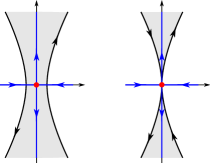
Recall the standard fact that a hyperbolic complex tangency of either sign has two unstable and two stable manifolds with this orientation convention, while positive (resp. negative) elliptic points have a two-dimensional unstable (resp. stable) manifold.
Lemma 2.1.
The surface obtained from by adding the cylinder described above has a characteristic distribution with only two singular points
which are hyperbolic points of opposite orientation signs. Furthermore:
-
•
The stable as well as unstable manifolds of for the characteristic distribution consist of a pair of integral curves; these two integral curves intersect the boundary of the cylinder in two different components, where this intersection is transverse in a single point.
-
•
Near the boundary of (which coincides with the boundary of the cylinder) the characteristic distribution coincides with in the above coordinates.
Proof.
The statements can be checked explicitly by investigating the characteristic distribution on ; see Figure 1 for a schematic picture of the characteristic distribution and the stable/unstable manifolds.
In addition, note that is a contact-form preserving isomorphism that fixes the cylinder set-wise, preserves its orientation, while it interchanges the two boundary components. Since this involution necessarily preserves the unstable and stable submanifolds, one immediately concludes that the pairs of integral curves of the stable (resp. unstable) submanifolds of intersect the boundary of in different components. ∎
at 106 116 \pinlabel at 221 49 \pinlabel at 117 75 \pinlabel at 117 36 \pinlabel at 117 -1

The above construction is an “ambient 0-surgery” (or self-connected sum) performed on the Lagrangian surface inside the contact manifold, yielding a natural embedding of the abstract manifold obtained from by surgery on the embedded 0-sphere . This construction will be called an ambient 0-surgery along the Legendrian arc with parameter . By the previous lemma, when is totally real, the produced surface has only hyperbolic complex tangencies; more precisely, there is one pair of hyperbolic points for each attached handle.
Example 2.2.
The Clifford torus
is totally real inside (it is even Lagrangian). The intersection is the standard Legendrian unknot, and it intersects the Clifford torus transversely in precisely the four points . In other words, this gives four different Legendrian arcs that we can use when performing the surgery construction. An application of the Reeb flow (i.e. multiplication by ) produces two -families of such arcs; each -family consists of pairwise disjoint arcs. Denote by
the genus- surface with precisely hyperbolic points obtained by performing an ambient surgery on arcs of the type described above. Note that, since already is pre-Lagrangian everywhere, we can already find the required normal neighborhood of the arc, without a further perturbation of the surface. (Recall that the perturbation was needed in order to make the surface pre-Lagrangian near the endpoints of the arc.)
The remaining part of the section will consist of analyzing holomorphic discs of Maslov index two inside with boundary on the genus- surface . The goal is to establish that is rationally convex by showing that these holomorphic discs constitute a holomorphic filling of the surface that satisfies certain additional properties.
2.1. Holomorphic fillings of a surgery on the Clifford torus
Recall that admits two fillings and by holomorphic discs of Maslov index two that are contained inside lines; these fillings are the two solid tori
that carry the holomorphic disc foliations
For sufficiently small in the above ambient surgery construction, we may assume that plenty of holomorphic discs in the above two families have boundaries that are contained inside the subset of the Clifford torus that is left undeformed by the surgery. Our goal is to show that these holomorphic Maslov-two disc live in moduli spaces that provide holomorphic fillings of the positive genus surface produced by the surgery. Moreover, the fillings produced on the surface of genus produced by the surgery will be seen to be given by a standard handle-body bounding that surface.
Denote by the union of the discs whose entire boundary is contained inside . For a carefully created surgery in a sufficiently small neighborhood, we may assume that is a disjoint union of a number of embedded solid cylinders with boundary on of the form
where consists of number of open intervals. When the above surgery may be assumed to produce a surface for which
consists of a disjoint union of number of embeddings of the connected compact surface of genus with four boundary components (i.e. a sphere with four open balls removed), and for which each connected component is totally real away from precisely two generic hyperbolic complex tangencies. Denote by , an enumeration of the connected components of .
Lemma 2.3.
After a generic -perturbation of supported away from the boundary, admits a holomorphic filling that coincides with near . Furthermore, the filling is diffeomorphic to a three-ball with four tubes attached. See Figure 2.
Proof.
Recall the famous result by Bedford–Klingenberg [BK91] by which any generic sphere inside a the boundary of a rationally convex four-dimensional domain with only good hyperbolic tangencies admits a filling that is diffeomorphic to a ball. We refer to the aforementioned paper for the definition of a good hyperbolic tangency, but note that any hyperbolic tangency can be -perturbed in an arbitrarily small neighbourhood in order to make it good.
Each genus-0 surface with boundary can be completed to an embedded sphere by adding discs with exactly one elliptic complex tangency at each of its four boundary components; e.g. take a perturbation of a radial projection of the holomorphic discs in to . The aforementioned results about fillings by holomorphic discs in four-dimensional symplectic manifolds implies that the spheres produced are fillable by holomorphic discs. A standard argument involving positivity of intersection then shows that this disc family necessarily coincides with the discs from the family near the boundary of .
Alternatively, one could just start with the disc families near themselves and run the argument of Bedford–Klingenberg to produce a filling, without passing to the auxiliary sphere.∎
We immediately conclude the following:
Corollary 2.4.
After a generic -small perturbation of support away from the discs in , this family extends to a holomorphic filling by discs of that is homeomorphic to a handle-body of genus .
at 40 45
\pinlabel at 40 80
\pinlabel at 155 83
\pinlabel at 275 45
\pinlabel at 275 80
\pinlabel at 155 40
\endlabellist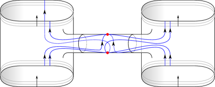
2.2. Graph structure of the moduli space of discs
In order to prove rational convexity we need to further analyze the fillings produced by Corollary 2.4. Recall that these fillings are given by the solutions in certain moduli spaces of holomorphic discs with boundary on the surface , which exist by the argument by Bedford–Klingenberg [BK91].
In [BK91] and [Eli90], the structure of the moduli space of discs on an oriented surface that constitute a filling was analyzed, and shown to be a directed graph with only vertices of valency one and three for a generic surface.
-
•
The edges parametrize one-parameter families of smoothly embedded Maslov-two discs with boundary on the surface, where the boundary of the discs are transverse to the characteristic foliation; Moreover, the edges are oriented so that agrees with the chosen orientation of the surface, where is a coordinate on the oriented edge, and is a coordinate on the boundary of the disc with the induced orientation.
-
•
The one-valent vertices correspond to elliptic complex tangencies and the edge is outgoing if and only if the elliptic point is positive (there are no such points for ); and
-
•
The three-valent vertices are in bijection with the hyperbolic complex tangencies, where the vertex is a nodal configuration that corresponds to a nodal configuration consisting of two holomorphic discs that are smooth away from the node. Moreover, the hyperbolic point is positive if and only if there are two incoming and one outgoing edge.
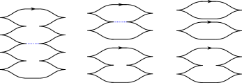
The discs at the incoming edge(s) approach the hyperbolic point from the outside (resp. inside) when the hyperbolic point is negative (resp. positive), according to the notation of [BK91]. See Figure 3.
With our orientation convention for the characteristic foliation, we obtain the following.
Lemma 2.5.
The orientation on the surface , which coincides with at any boundary point of a smooth holomorphic disc in the above moduli space as described above, coincides with , where is a one-form for which , an such that induces orientation of the characteristic distribution according to our convention.
Proof.
Recall that the filling is constructing by applying the argument by [BK91] to spheres obtained by closing up the surfaces . These fillings, in turn, are obtained from continuing the Bishop families near elliptic complex tangencies. The statement can be checked to hold near these Bishop families. Since the discs families remain transverse to the characteristic foliation away from the finitely many nodes, the property remains true for all smooth discs. We also get the same result for the filling of itself. ∎
Lemma 2.6.
The graphs corresponding to the moduli spaces that fill a component are either Configuration (a) or (b) shown in Figure 4, where (a) consists of two incoming (resp. outgoing) families from the discs in at the positive (resp. negative) hyperbolic point.
Proof.
Fist note that the filling of given by Lemma 2.3 coincides with four components of discs from near its boundary; two of these components correspond to edges oriented into the , denoted by , while two are oriented out from , and are denoted by .
It is now simply a matter of enumerating all directed graphics with two three-valent vertices, two incoming leaves, and two outgoing leaves. ∎
at 60 15
\pinlabel at 60 75
\pinlabel at 0 75
\pinlabel at 42 57
\pinlabel at 42 30
\pinlabel at 143 57
\pinlabel at 160 57
\pinlabel at 110 35
\pinlabel at 110 60
\pinlabel at 195 60
\pinlabel at 195 35
\pinlabel at 0 15
\pinlabel at -20 45
\pinlabel at 85 45
\endlabellist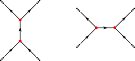
In order to prove rationally convexity of we need to sharpen the result of Corollary 2.4 to the following structural result by excluding Configuration (b) from appearing; see Figure 4.
Proposition 2.7.
The holomorphic filling by disks of produced by Corollary 2.4 is a genus handle body that contains the disc family as a sub-filling, and for which
-
•
the vertices in the moduli space are all three-valent and in bijective correspondence with the number of hyperbolic complex tangencies;
-
•
any oriented edge in the moduli space can be extended to an oriented cycle in the graph.
The moduli space is the graph shown in Figure 5; note that the pair of hyperbolic points that are contained inside the same handle are connected by a pair of oriented edges that share the same start an endpoints.
Proof.
Lemma 2.1 shows that any unstable (resp. stable) manifold inside the cylinder inside any connected component that is associated to a singular point intersects the boundary in two different components. Using the fact that the characteristic distribution of is tangent to the vector-field generated by the standard action of by scalar multiplication on , which is everywhere transverse to the standard disc family , we conclude that the unstable (resp. stable) manifolds of intersect the boundary of transversely in a unique point.
This means that the discs in the family , whose boundaries foliate a neighborhood of the boundary of , and which enter the surface cannot be a part of the unique incoming edge of the negative hyperbolic point. Namely, such a disc would necessarily intersect both stable manifolds of the hyperbolic point; see Figure 3. This excludes the possibility of Configuration (b), and we are thus left with Configuration (a) as sought. ∎
at 48 34
\pinlabel at -10 13
\pinlabel at 85 34
\pinlabel at 120 34
\endlabellist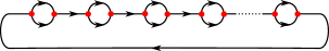
2.3. Holomorphic fillings of a surgery on a knotted rationally convex torus
In this section we provide two approaches for constructing rational convex high genus surfaces in whose smooth isotopy class inside the sphere differs from the constructed in Section 2.1. Note that the latter surface is unknotted in the sense that it creates a Heegaard-splitting of into two handle-bodies.
Take any transverse knot inside . This knot can be taken to live in any smooth isotopy class. Recall that the standard neighborhood theorem of transverse knots implies that it has a solid torus neighborhood that is foliated by pre-Lagrangian tori collapsing on the transverse knots. In particular, these tori are totally real, and have a complement that consists of one component that is a solid torus. If the original transverse knot is knotted, then the other component is not a solid torus.
Lemma 2.8.
These pre-Lagrangian tori admit filling by embedded holomorphic discs in whose projection to is equal to the solid torus that is bounded by the torus.
Proof.
Cut the torus open along a compressing disc in order to form a sphere with precisely two generic elliptic complex tangencies, and then consider the filling provided by [BK91]. ∎
The rest of the construct can be performed as in Section 2.1, yielding an embedded genus- surface with precisely number of hyperbolic complex tangencies, which admit holomorphic fillings by discs with the same properties as those in Proposition 2.7. Note that the Legendrian arcs needed for the surgery can be constructed explicitly e.g. inside the solid torus neighborhood of the transverse knot.
Alternatively, one can also start with the surface given by the Clifford torus as above, but then choose the Legendrians arcs along which the surgery is performed to be knotted.
2.4. Rational convexity of (Proof of Theorem 1.1)
Here we prove the rational convexity of the fillable genus- surfaces of the type constructed in either of Sections 2.1 and 2.3.
This argument follows as the proof of rational convexity for fillable tori in [DG14, Section 1.b]. We repeat it here for completeness. First we show that the filling itself is rationally convex.
Lemma 2.9.
Proof.
By pushing off in its normal direction inside , we can create an open neighborhood of that is foliated by genus- surfaces, each of which has only isolated hyperbolic complex tangencies. A standard argument implies that the filling persists under these deformations, and thus produces a smoothly varying family of fillings of these disjoint surfaces. Positivity of intersection implies that two fillings for two disjoint surfaces in the family are disjoint. In conclusion, these fillings foliate an open neighborhood of .
We have shown that any point in that lives in a sufficiently small neighborhood of lies on a holomorphic disc that is disjoint from the filling , where this disc has boundary contained in . This Riemann surface can be approximated by the zero-set of a polynomial that does not vanish on the filling. The statement follows from this. ∎
Then we finish by producing analytic varieties that pass through the discs in the filling, and which do not pass through the surface in , thus excluding the interior of the discs in the filling from the rational hull.
Lemma 2.10.
Proof.
The holomorphic fillings of constructed in the aforementioned subsections has the following property: Any point inside of the filling that is disjoint from the boundary lies in a smoothly embedded closed curve inside the filling that is disjoint from the boundary , while it intersects any disc in the filling transversely. This curve can be extended to a small holomorphic annulus that intersects the filling near the core of the annulus.
Since the filling is rationally convex by Lemma 2.9, we can approximate it by a domain of holomorphy. Then we can run the same argument as in the proof of the previous lemma; namely, the annulus extends to a properly embedded algebraic curve in that is disjoint from . The existence of this analytic variety implies that , as sought. ∎
∎
3. Symplectic condition for rational convexity
A famous result by Duval–Sibony [DS95, Theorem 3.1] states that any totally real half-dimensional submanifold is rationally convex if and only if it is Lagrangian for some global Kähler form on (which in fact can be taken to be equal to the standard linear outside of a compact subset). Here we provide a generalisation of this result in the case to surfaces that have a finite number of complex hyperbolic tangencies in addition to the totally real locus. Recall that generic complex tangencies are either hyperbolic or elliptic, and that elliptic complex tangencies are an obstruction to rational convexity.
A surface that has a complex tangency can of course not be Lagrangian for a Kähler form. However, the condition that ensures rational convexity is, roughly speaking, that the surface is Lagrangian for a Kähler form that is degenerate precisely at the complex tangencies. To that end, we use Shafikov–Sukhov’s adaptation [SS16, Lemma 2] of Gayet’s condition for rational convexity from [Gay00]. Another crucial ingredient that we rely on is the local Stein neighborhood basis of a surfaces with only flat hyperbolic complex tangencies that was constructed by Slapar [Sla04].
Theorem 3.1.
Let be a smooth compact surface that is totally real outside of a finite number of flat hyperbolic tangencies . Assume that is Lagrangian for a global Kähler form on , which near can be written as , where satisfies
-
•
, and vanishes precisely at ;
-
•
in where is some neighbourhood of the hyperbolic points; and
-
•
vanishes on .
Then is rationally convex.
Proof.
By the Slapar’s result [Sla04, Theorem 2] we can find a plurisubharmonic function defined in some neighborhood of that has the property that , and where is strictly plurisubharmonic away from the hyperbolic tangencies . We extend to a smooth and compactly supported function defined on all of .
Consider the global plurisubharmonic function produced by Lemma 3.2, and consider the function
By construction, is pluriharmonic in a neighborhood of the hyperbolic tangencies and strictly plurisubharmonic in . If we take sufficiently large, the plurisubharmonic moreover becomes strictly plurisubharmonic on all of .
Rational convexity is then a consequence of [SS16, Lemma 2] or [Gay00, Lemme 1]. We proceed to show that the necessary conditions are satisfied, so that he result can be applied.
A standard argument shows that, after perturbing away from , while keeping the Lagrangian property of , we may further assume that for some smooth ; see e.g. [SS16] or [Gay00]. We then consider the function defined on .
First, we claim that is satisfied along for some holomorphic function . Indeed, holds along , since the latter is a critical manifold of the function . Since is pluriharmonic in , we can write there, where . Further, holds up to a constant, since along .
Second, we use Hörmander–Weber’s result [WH68, Lemma 4.3] to extend the holomorphic function defined on to a function defined in a neighborhood of , where further
-
•
; and
-
•
for some arbitrary .
Since is satisfied along by construction, the second bullet point above implies that the functions and agree to the first order along .
Third, after cutting off by a bump function supported in some small neighborhood of the inequality can be assumed to hold globally, with equality precisely along . Indeed, inside we have and since is positive away from in , we thus get in with equality precisely on . To show the inequality in a sufficiently small neighborhood of we argue as follows. The function can be assumed to be strictly plurisubharmonic on . After shrinking further, a standard argument implies that holds everywhere in , with equality precisely along .
This establishes all assumptions needed in order to apply [Gay00, Lemme 1], which then shows that is rationally convex. ∎
Lemma 3.2.
Consider the Kähler form that is non-degenerate outside and which satisfies the assumptions of Theorem 3.1. For any sufficiently small open neighborhood of , there exists a global plurisubharmonic function that
-
•
is pluriharmonic in sufficiently small closed neighborhoods of ;
-
•
is strictly plurisubharmonic in and satisfies in ; and
-
•
satisfies the property that along .
Proof.
Consider the non-negative plurisubharmonic function defined near with the properties prescribed by Theorem 3.1; without loss of generality we may assume that is defined on the open neighborhood . In particular, holds on .
Post-composing the plurisubharmonic function with a suitable convex function that vanishes in , we obtain a plurisubharmonic function that
-
•
vanishes in the closed neighborhood of the hyperbolic points, where we may assume that after taking sufficiently small;
-
•
is strictly plurisubharmonic in , while moreover holds outside of a compact subset of ;
-
•
still satisfies the property that is locally constant near the hyperbolic points when restricted to .
Denote by the globally defined smooth -form that coincides with in and with in . The -lemma then provides the sought global plurisubharmonic function for which . ∎
3.1. The converse statement: rationally convex are singular Lagrangians
We then prove a converse to Theorem 3.1, by showing that any rationally convex surface with standard flat hyperbolic tangencies can be made Lagrangian for a symplectic form that degenerates precisely at the hyperbolic points.
Theorem 3.3.
Assume that is a smooth surface that is rationally convex and totally real except for a finite number of standard flat hyperbolic complex tangencies. There exists a smooth -form on which is Kähler on for which is Lagrangian.
Proof.
The proof is completely analogous to the case when is totally real, which is due to Duval–Sibony [DS95, Theorem 3.1].
The rational convexity of implies that there is a smooth function for which is positive on , while it vanishes precisely on . See [DS95, Remark 2.2].
The sought Kähler form can then be taken to be where is sufficiently small, and is the plurisubharmonic function defined in some neighbourhood of that was constructed by Slapar in [Sla04, Theorem 2]. ∎
4. Lagrangian model of a complex hyperbolic tangency
The goal of this section is to construct a local model of a hyperbolic complex tangency in together with a Kähler form that is degenerate precisely at the tangency, and for which the local model becomes Lagrangian. This construction will then be used as a building block for surfaces that satisfy the assumptions of Theorem 3.1, and which thus are rationally convex.
The hyperbolic tangency that we consider is of the particular form
in local holomorphic coordinates on . We will call such points standard hyperbolic complex tangencies. Note that this hyperbolic complex tangency is not “good” in the sense of [GS12], but it can be approximated by hyperbolic tangencies that are good. More importantly, this complex hyperbolic tangency is “flat” in the sense of Slapar [Sla04].
4.1. Local symplectic description of the hyperbolic tangency
We begin with a local description of the hyperbolic tangency from a symplectic viewpoint. Our description is close to that of Nemirovski–Siegel in [NS16, Section 4.3], where it was shown that the Legendrian unknot of and bounds a disc with a single hyperbolic complex tangency inside the standard ball . This Legendrian unknot has a representative with the front projection depicted in Figure 6.
at 1 90
\pinlabel at 1 195
\pinlabel at 223 42
\pinlabel at 223 105
\endlabellist
Next we give a description of the local model in terms of the coordinates induced by the standard momentum map
These coordinates also turn out to be useful for constructing the locally defined plurisubharmonic functions that we will need.
Consider the torus knot
which is entirely contained inside the toric fibre over and actually smoothly unknotted. Its cone is Lagrangian with an isolated singularity at the origin, from which we deduce that is Legendrian. The -torus knot is smoothly unknotted. However, it is not Legendrian isotopic to the standard Legendrian unknot of , but rather Legendrian isotopic to the once stabilised Legendrian unknot shown in Figure 6. This fact can be seen either by an explicit construction or, alternatively, deduced from the classification of Legendrian unknots [EF09] by Eliashberg–Fraser. Recall that the Legendrian isotopy class of unknots in the standard contact sphere are completely classified by its rotation number (which is ) together with Thurston–Bennequin invariant (which is ).
Next we deform the cone near the origin in order to smooth it to a single flat hyperbolic complex tangency. First we consider the image of this cone under the momentum map; it is the dashed line with slope depicted in Figure 7. Note that the cone is not the full pre-image of the line; each fibre consists of the linear sub-torus that corresponds to the normal of the line in the momentum polytope.
We then consider the surfaces of the form
and note that this surface coincides with the the aforementioned cone precisely when We define to be equal to for a smooth function that satisfies
-
•
near ;
-
•
for ;
-
•
for all ; and
-
•
for all .
In particular, this means that has a standard hyperbolic complex tangency at the origin. To see this, we begin with the straight forward identification of and the graph
near the origin. After the coordinate change , this graph can be expressed as
This is the so-called standard quadratic hyperbolic tangency, which in particular is “flat” in the sense of [Sla04].
The next step is to construct a smooth plurisubharmonic function which is strictly plurisubharmonic outside of the origin, and for which becomes Lagrangian inside the same subset. In order to do this we first need to describe some useful tools for constructing such a function. We will use polar coordinates , describe the function through with . We compute
Note that, in these coordinates, we can write for as described above.
-
•
Making Lagrangian: The condition for to vanish on is that the gradient is orthogonal to
along the subset or, equivalently, that the gradient is colinear with
along the same subset. (The curve shown in Figure 7 is the projection of under the momentum map ).
-
•
Making plurisubharmonic: Since , a direct calculation implies that the function is strictly plurisubharmonic at all points where the inequalities
are satisfied simultaneously for In particular, this is automatically the case when as well as are satisfied for .
Furthermore, at a point where holds simultaneously for both , strict plurisubharmonicity can be achieved by post-composing with a convex function for which , , and where is sufficiently large at . Indeed, the second derivative of satisfies
-
•
Condition for obtaining the standard symplectic form: When , it is clear that is strictly plurisubharmonic outside of the origin whenever and hold in the same subset. Recall that gives the standard symplectic form .
at 103 -8
\pinlabel at 128 5
\pinlabel at 11 118
\pinlabel at 72 -8
\pinlabel at -8 37
\pinlabel at -8 68
\pinlabel at -2 100
\pinlabel at 40 -8
\pinlabel at 53 17
\endlabellist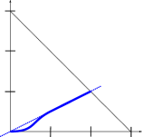
at 103 -8
\pinlabel at 128 5
\pinlabel at 11 118
\pinlabel at 72 -8
\pinlabel at -8 37
\pinlabel at -8 68
\pinlabel at -2 100
\pinlabel at 40 -8
\pinlabel at 53 17
\endlabellist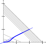
The following technical result will be important for establishing the conditions in [Gay00, Lemme 1], which is a result that we invoke to show rational convexity.
Proposition 4.1.
There exists a smooth plurisubharmonic function that satisfies
-
(1)
near ;
-
(2)
is strictly plurisubharmonic in ;
-
(3)
has no critical points in , and its level sets are transverse to in the same subset; and
-
(4)
the one-form vanishes on . In particular, is an exact Lagrangian submanifold that, for each , intersects the contact hypersurfaces
in Legendrian knots.
Proof.
We start by constructing a smooth function defined on the first quadrant of the -plane whose gradient is orthogonal to along the curve , and such that is satisfied away from the origin .
First consider the foliation of the first quadrant by the lines
where parametrizes the leaf space (i.e. the space of lines), and parametrizes each leaf (i.e. line). Note that the line with parameter value passes through the point when with tangent vector .
The line corresponding to the parameter-value intersects the first and second coordinate axis at the points (when ) and (when ), respectively. Recall that holds with strict inequality for . Since the -derivative of this family of lines thus is everywhere non-zero when and , we conclude that this is a smooth foliation away from the origin.
The foliation property allows us to find a continuous function defined in the first quadrant , which is smooth away from the origin, and whose level-sets constitute the above foliation by lines. We define uniquely by the requirement that it takes the value along the leaf with parameter value .
The sought plurisubharmonic function that is strictly plurisubharmonic away from the origin will be obtained by setting and considering the composition for a suitable function with and for .
Property (1): Since when , we get the equality in the subset with our convention. We thus need to hold in the subset .
Property (2): First we need to investigate the behavior of the partial differentials of near the origin , which is precisely where the smoothness fails. Since holds near , each level set can be parametrized by
near the origin. It follows that
which is a function that is smooth away from the origin, and whose partial differentials can be bounded from above by functions of the form
| (4.1) |
for depending on the order of the partial differential.
For any smooth function which satisfies , near for some , , and all , one readily computes that is smooth in all of Here we need Inequality (4.1) for bounding the growth of the the partial differentials of . A function satisfying this property can be obtained by specifying
where satisfies for all close to , and . Furthermore, we will take the function to satisfy near . It follows that for , for all , and that is everywhere . Furthermore, we have near . The latter means that is still satisfied near .
After choosing to be sufficiently large away from some neighbourhood of which, in particular means that we must choose sufficiently large, we obtain the strict inequalities
| (4.2) |
away from the origin. To that end, recall that the gradient has positive components away from the origin, and that Inequality (4.1) controls their growth near the origin. Since , when combined with the second bullet point before this proposition, Inequality (4.2) implies that is strictly plurisubharmonic away from the origin.
Property (3): Note that the gradient is orthogonal to the tangent vectors of the level-sets of , which by construction is the tangent vectors to the family of lines constructed above. Hence, the gradient is co-linear with . In particular, since holds away from the origin, both components of the gradient are positive in this subset. It also follows that the level sets are transverse to . The same is then true for the composition .
Property (4): The first bullet point in the paragraph before this proposition, together with the calculation of the gradient , ensures that vanishes when pulled back to . The same is then true for the composition . ∎
4.2. Digression: Results about Lagrangian fillings of .
For completeness, we here investigate some properties satisfied by the Lagrangian fillings of the stabilised Legendrian unknot . There are implications for the possible smoothings of the singular Lagrangian cone over the Legendrian knot shown in Figure 6.
-
(1)
The Legendrian does not bound any orientable Lagrangian submanifolds simply for the purely topological reason that . Hence, the singularity at the origin of the Kähler form produced by Proposition 4.1 cannot be avoided. Without a singularity, we would have produced a Lagrangian disc filling of inside the symplectic ball.
-
(2)
The Legendrian also does not bound any non-orientable exact Lagrangian fillings (recall that exact means that has a primitive which pulls back to an exact one-form on the Lagrangian). Unlike (1) above, the proof of this fact uses harder techniques than just classical homotopy theory. The Legendrian contact homology of the knot , i.e. the Legendrian isotopy invariant in the form of a differential graded algebra (DGA) defined by Chekanov in [Che02], is acyclic with -coefficients. An exact Lagrangian filling would imply the existence of an augmentation of this DGA, i.e. a unital DGA-morphism to the ground field ; see e.g. [CCPR+22].
-
(3)
The Legendrian knot does, however, bound non-orientable Lagrangian fillings by the h-principle for Lagrangian immersions. Namely, the h-principle provides Lagrangian immersions with generic double points. The latter double points can be removed by a Lagrangian surgery [Pol91]. Recall that performing surgery on several double points typically produces a non-orientable Lagrangian.
A more explicit construction can be made as follows. Perform ambient Legendrian surgeries on as defined in e.g. [DR16] to yield an exact Lagrangian cobordism to a link of standard unknots; see Figure 9. This cobordism has at its concave end and the link of unknots at its convex end. The direction of this cobordism can be reversed, with the cost of adding double points. The reversed immersed cobordism now has two Legendrian unknot components at the concave end; they can be filled by two Lagrangian discs, which intersect since the unknots are linked. Finally, we smooth all double points on the immersed Lagrangian cobordism, which yields a non-exact non-oriented Lagrangian filling.
-
(4)
The Legendrian does not bound a Lagrangian Möbius band. The reason is that the primitive of the symplectic form, which is exact near the Legendrian boundary, would automatically be exact on the entire Lagrangian Möbius band; namely, the restriction of -cohomology classes to the boundary is an isomorphism when -coefficients are used. Or put differently: any Lagrangian Möbius band is automatically exact, which is not allowed by (2) above.
However, there exists Lagrangian Möbius bands which are non-exact and non-compactly supported Lagrangian deformations of the cone over . In other words, this is a non-exact Lagrangian filling that is not cylindrical, but merely asymptotic to the Legendrian knot at infinity. Such a Lagrangian Möbius band is given by
for , whose core is the circle contained in the second coordinate plane. (In particular, there is a holomorphic Maslov-0 disc with boundary on this filling.) Note that this Lagrangian is asymptotic to the cone over , but that it is neither conical nor exact outside of a compact subset.

Remark 4.2.
The non-exact Lagrangian asymptotic fillings of the Legendrian knot in (4) above can be used to deform the genus- surfaces produced by Theorem 5.1, which are Lagrangian outside a number of standard models of hyperbolic points, to yield an embedded Lagrangian surface with the hyperbolic points replaced by a number of Lagrangian Möbius bands. However, since the Möbius band constructed in (4) does not coincide with the cone over the Legendrian near its boundary – rather, it is a non-exact deformation of this cone – we must perform a non-local perturbation of the initial Lagrangian in order for the Lagrangian Möbius bands to fit in the model. The necessary deformation of the Lagrangian surface can readily be carried out by the fibre-wise addition of a suitable non-exact closed one-form inside its standard Weinstein neighborhood.
5. Non-fillable rationally convex surfaces with only hyperbolic tangencies
It is a standard fact that a closed surface of genus that is totally real except for hyperbolic tangencies satisfies
This can e.g. be seen by computing the self-linking numbers of the knots defined by intersecting the complex tangencies by small round spheres for the framing defined by the Reeb vector field on the round contact sphere , where . In this section we construct non-fillable rationally convex surface in of genus with a number of hyperbolic complex tangencies.
The construction of these surfaces can roughly be outlined as follows. We start with an exact Lagrangian genus- surface inside that is embedded away from a number of conical singularities of the form described in Subsection 4.1. Recall that the singularity considered in the aforementioned section is a cone over the Legendrian unknot of shown in Figure 6. It should be noted that the existence of exact Lagrangians with all singularities of this particular type is non-trivial; they were first constructed by Lin in [Lin16], whose construction is related to earlier work by Sauvaget [Sau04]. Then we replace each cone-point with a smooth disc which has a unique hyperbolic complex tangency, a construction which also was described in Subsection 4.1. The concatenation of the Lagrangian and the disc with hyperbolic complex tangencies is depicted schematically in Figure 10. The construction yields the following:
Theorem 5.1.
There exists smooth surfaces of any genus that satisfy:
-
•
There exists a union a number of disjoint round Euclidean Kähler balls
where coincides with the standard disc model from Subsection 4.1 inside each ball. (In particular, in each ball has a single flat hyperbolic complex tangency, and it is Lagrangian for the Kähler form that is degenerate precisely at the tangency); and
-
•
Using to denote the smooth -form on that coincides with in each Darboux ball in and with in , then is exact for any choice of primitive of . In particular is an exact Lagrangian submanifold away from the hyperbolic points.
Proof.
Start with a number of disjoint copies of the round closed Darboux balls , e.g. obtained by applying affine transformations to one standard Euclidean ball, and denote by their union. The components of will be denoted by .
In each boundary , which is a round contact sphere, we place one copy of the unknot of and . See Figure 6 for the front projection of this knot when placed inside a small contact Darboux ball by a contact isotopy. However, we will use the representative of its Legendrian isotopy class as described in Subsection 4.1, i.e. given as a sub-torus in the standard momentum polytope. To see that these knots are the same up to Legendrian isotopy, one can e.g. use the fact that unknots inside the standard contact sphere are classified by their classical invariants and ; see [EF09]. Finally, denote by the union of these Legendrian knots.
Perform a number of standard Weinstein 1-handle attachments in order to connected the symplectic Darboux balls to form a connected ball . These handle-attachments form an abstract compact Weinstein cobordism from to . For very thin Weinstein 1-handles the resulting Weinstein cobordism admits a symplectic embedding into , with concave end coinciding with the boundary of our original domain . We refer the reader to [CE12], but also provide the following rough outline of a construction:
The Weinstein 1-handles are locally determined by the corresponding isotropic core disks, which constitute the skeleton of the cobordism. The core disks are the 1-dimensional isotropic discs defined as the stable manifolds of the critical points of the Liouville vector field on . The embedding of can then be constructed as follows. First, we embedding a number of isotropic arcs with boundary transverse to . Second, we identify with by choosing a smooth identification of with . Finally, this identification can be extended to a smooth symplectomorphism of a neighbourhood of into .
By the previous paragraph the cobordism can be identified with a symplectic embedding , whose convex boundary
thus is a contact-type hypersurface in ; this contact manifold is contactomorphic to the standard contact 3-sphere. (Note that the contact form that is induced by the primitive of typically is not equal to the round contact form, but this will not be important here.) The concave boundary of the cobordism is the disjoint union of a number of standard round contact spheres.
The endpoints of the unstable manifolds , i.e. the attaching -spheres of the Weinstein 1-handles, can be assumed to be disjoint from the Legendrian knots contained in the concave boundary of the cobordism . Furthermore, since the complement of a point in the standard contact sphere is contactomorphic to a Darboux ball (see e.g. [Gei08]) we can assume that is contained in a union of contact Darboux balls that are disjoint from the attaching spheres.
Using the Liouville flow defined by in the Weinstein cobordism we obtain an exact embedding of the cylinder
Inside this trivial symplectic cobordism, we can embed the trivial Lagrangian cobordism with convex cylindrical end equal to a union of a number of -knots contained in disjoint contact Darboux balls in the contact sphere . Note that this trivial Lagrangian cobordism is tangent to the Liouville vector field of by construction.
We then use Lemma 5.6 to extend the embedding of to a symplectic embedding of
where is the original embedding of , and where is contained inside the unbounded component of the complement . Adjoining the above embedding to produces a symplectic embedding
of the completion of .
We are now ready to construct the surface which will be exact Lagrangian outside of the hyperbolic points.
A disc inside : Here we use the model from Subsection 4.1 in each component of . The components are the discs with one complex hyperbolic tangency, which is Lagrangian for away from these tangencies.
A trivial cylinder in : Here we use the trivial Lagrangian cobordism that is tangent to the Liouville vector field.
A Lagrangian handle-attachment inside : First we perform a Legendrian isotopy to make the union of Legendrian unknots equal to the standard representatives shown in Figure 6 horizontally aligned next to each other. There is an associated exact Lagrangian trace cobordism.
Then we perform a number of ambient Legendrian surgeries as defined in e.g. [DR16] on , thus yielding a single component Legendrian unknot ; see Figure 10 for the case . There is an associated exact Lagrangian cobordism that consists of the corresponding standard Lagrangian one-handles. This Lagrangian cobordism lives in
and has a concave end consisting of the unlinked unknots and a convex end the connected unknot . Note that the Lagrangian cobordism is diffeomorphic to a sphere with discs removed. We refer to [DR16] for an explicit description of its construction.
Capping off : The final piece is the most involved part of the construction, and consists of adjoining an exact Lagrangian cobordism in of genus with concave end . Here we rely on Lin’s construction in [Lin16]. Since we later want to understand the smooth isotopy class of the filling we proceed to give some details.
In the simplest case , i.e. when there are exactly two hyperbolic tangencies, the construction of the exact Lagrangian is depicted in Figure 10. When , we perform a sequence of ambient surgeries along unknotted arcs to produce an exact Lagrangian cobordism of genus from to . This is obtained by first performing a number of suitable ambient Legendrian surgeries to produce an exact Lagrangian cobordism from to a union of unlinked Legendrian unknots: one copy of and copies of the standard Legendrian unknot ; see Figure 11 for the case . Then, we perform ambient Legendrian surgeries from the latter link of Legendrian unknots to by taking connected sum with the standard Legendrian unknots. (Recall that a cusp-connected sum with a standard Legendrian unknot does not change the Legendrian isotopy class of the second knot.) The resulting cobordism has genus . Finally, we adjoin Lin’s exact Lagrangian cobordism of genus 2 to the Legendrian knot .
The exactness of is immediate. Take any global primitive one-form of the two-form . Since is closed on the pull-back , it is moreover exact on the discs . Since on , it follows that for some closed one-form on the same domain. Since is simply connected, we get that is exact. Since is exact by construction, it then follows that is exact as well. ∎
A direct application of Theorem 3.1 above gives that
Corollary 5.2.
The surfaces with only hyperbolic complex tangencies as constructed by Theorem 5.1 are all rationally convex.
The surfaces produced by Theorem 5.1 are all exact in the following sense:
Definition 5.3.
An embedded submanifold is said to be exact totally real or just exact if there exists a Kähler form which is non-degenerate away form a compact totally real embedding , and for which is an exact one-form.
A famous result by Gromov [Gro85] implies that no real -dimensional closed manifold is exact for a Kähler form that is non-degenerate on all of . An immediate consequence of Stokes’s theorem is that
Lemma 5.4.
Every compact Riemann surfaces with boundary attached to an exact submanifold must be constant.
Proof.
Stoke’s theorem implies that the -area of the Riemann surface must vanish. However, unless it is constant, it must intersect the non-degenerate locus in a non-empty subset. This contradiction shows that the map indeed must be constant. ∎
In other words, the surfaces produced by Theorem 5.1 do not admit holomorphic fillings in the following very strong sense.
Corollary 5.5.
Any continuous map from a Riemann surface into with boundary on a rationally convex surfaces produced by Theorem 5.1 must be constant, under the assumption that the Riemann surface is compact, and that the map is holomorphic away from the boundary.
We end with an auxiliary lemma about contact hypersurfaces in standard symplectic . Recall that a primitive of a symplectic form gives rise to the Liouville vector field defined by .
Lemma 5.6.
If is a closed hypersurface that satisfies which is of contact type, i.e. admits a primitive one-form near whose Liouville flow is transverse to , then there exists a symplectic embedding of the so-called symplectization
whose restriction to is the original embedding of , and where is the contact one-form on .
Proof.
Any two primitives of differ by a closed one-form near . Since , this one-form is exact, and we can thus extend to a global primitive of on that coincides with the standard primitive of outside of a compact subset. One can then readily use the Liouville flow in order to construct the sought symplectization coordinates. The Liouville flow is complete since the primitive of the symplectic form is given by outside of a compact subset. ∎
at 30 20
\pinlabel at 100 20
\pinlabel at 65 98
\pinlabel at 158 145
\pinlabel at 170 83
\pinlabel at 170 41
\pinlabel at 170 26
\endlabellist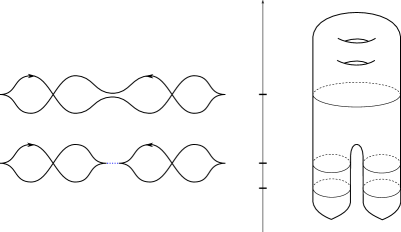
6. Constructing knotted rationally convex surfaces
Here we construct examples of smoothly knotted surfaces in that are rationally convex and which are exact with only hyperbolic complex tangencies. A closed embedded surface in that bounds an embedded three-dimensional handle-body is called unknotted. Recall that the smooth isotopy classes of surfaces in form a very rich structure, that can be detected using the fundamental group of the surface complement. The set of such fundamental groups are as rich as the knot groups of one-dimensional knots in , while the complement of an unknotted surface is equal to by a direct computation; see e.g. [DR24, Lemma 3.1].
First we show that
Proposition 6.1.
The rationally convex surfaces with only hyperbolic tangencies constructed in the proof of Theorem 5.1 all bound embedded three-dimensional handle-bodies; i.e. they are unknotted.
Proof.
In order to produce the required handle-body that bounds the surface, i.e. establish unknottedness, it suffices to show the existence of a proper Morse function with a unique critical point – a local minimum – for which the following is satisfied:
-
•
is disjoint from the critical point of and the restriction to the surface is Morse;
-
•
the intersection is a union of unlinked unknots for all regular values of ;
and, most importantly,
-
•
the unlinked unknots in the regular levels of bound a smoothly varying embedded union of discs inside that become pinched or split exactly at the critical points of .
Note that any surface can be put in a position satisfying the first two bullet points; it is only using the last bullet point that we can ensure unknottedness. The mechanism that we will use to ensure that the last bullet point holds is that
-
•
the regular slices have a smooth family of knot projections to under which two different components have disjoint images, and where each image of a component moreover is contained in the unbounded component of the complement of the others.
Next we produce such a Morse function for the surface . Recall that this surface can be decomposed into an unknotted disc contained inside the smooth ball , together with a genus- surface contained inside ; we refer to the proof of Theorem 5.1 for the construction of the ball .
It is easy to construct the sought Morse function inside the smooth ball . What remains is to check that this Morse function extends to a proper Morse function to the complement
of the ball, such that the restriction to satisfies the last bullet point above.
We claim that the sought Morse function on can simply be taken to be the symplectisation-coordinate . It can be seen explicitly by our construction that the part of the Lagrangian cobordism that we construct using explicit Legendrian ambient surgeries in the proof of Theorem 5.1 has knot projections with the required properties; see e.g. the front projections Figures 10 and 11.
The top piece of , i.e. the exact Lagrangian genus-two cap produced by Lin in [Lin16] also consists of slices whose knot projections satisfy the sought properties, as can be seen by inspecting [Lin16, Figures 23, 24 and 25] in his construction; these figures depict knot projections of the generic slices of his surface, and they clearly satisfy the property of the last bullet point above. ∎
We then show that the surface produced by Theorem 5.1 can be deformed in order to yield rational convex surfaces in different knot classes, under the assumption that is sufficiently large.
Theorem 6.2.
For each fixed sufficiently large, there exist several non-isotopic embeddings of the genus- surface inside which all are rationally convex, exact, and have only hyperbolic complex tangencies. Moreover, for any , we the fundamental groups of the complements of these different embeddings can be assumed to live in pairwise different isomorphism classes.
This result should be contrasted to the case of rationally convex surfaces in which are totally real and orientable; these are all tori that are smoothly unknotted by work of the first author joint with Goodman and Ivrii [DRGI16].
Corollary 6.3.
There are non-orientable surfaces that admit several Lagrangian embeddings in that are different when considered up to smooth isotopy. (Recall that these embeddings in particular are totally real and rationally convex by [DS95].)
Proof of Corollary 6.3.
Each hyperbolic point is contained inside a small four-ball, the union of which we denote by , such that the surface outside of the union of four-balls is Lagrangian for the standard symplectic structure . Furthermore, the intersection is a union of unknotted discs that intersect the boundary components of (i.e. a disjoint union of standard contact spheres) in Legendrian unknots.
We claim that it is sufficient to replace the unknotted discs in with non-orientable surfaces that are Lagrangian for the standard symplectic form , coincide with near , and which are unknotted in the sense that they bound a handle-body with a half-disk removed. More precisely, we want there to exist a handle-body in whose boundary intersects precisely in the Lagrangian surface. In particular, it follows that the complement of the surface inside the ball has fundamental group (which is isomorphic to the fundamental group of the complement of the unknotted disc).
The sought non-orientable Lagrangian surface can readily be constructed using Item (3) in Subsection 4.2. The knottedness then follows by a computation of the fundamental group of the complement of the non-orientable Lagrangian constructed using the Seifert–van Kampen theorem. ∎
Proof of Theorem 6.2.
Recall that the construction of the rationally convex surface in the proof of Theorem 5.1 is carried out by adjoining an exact Lagrangian cap of genus to a Legendrian unknot of and with positive and negative stabilisations. More precisely, by construction
is contained inside a contact-type hypersurface in that is the boundary of a 4-ball ; see the proof of Theorem 5.1. Moreover, the piece of the surface contained in the ball is an unknotted disc with hyperbolic complex tangencies, while the genus- cap is an exact Lagrangian that lives in the complement of the ball.
By construction, we may assume that the surface coincides with the Lagrangian cylinder
in symplectization coordinates defined near the contact-type hypersurface . In fact, here we may assume that is arbitrarily large, since we can perform a suitable rescaling of the symplectic form near as well as in the unbounded region of by an application of the Liouville flow.
The smooth isotopy class of will be altered by replacing the trivial concordance with a knotted Lagrangian concordance that coincides with the original trivial cylinder near its boundary.
By the construction of [DR24, Theorem 1.2] we can find such knotted Lagrangian concordances
whose complement has the fundamental groups of any given finite subset of the set of knot groups for 1-knots in , under the assumption that we take to be sufficiently large. The reason for this is that the construction needs sufficiently many stabilisations of both signs of the Legendrian knot involved; in our case has positive and negative stabilizations. Since the original surface bounds a handle-body, the fundamental group of the complement of the new deformed surface is the same as the fundamental group of complement of the concordance, which agrees with the given knot group; see [DR24, Corollary 3.4]. (The latter result was formulated for tori, but the proof is the same also in the case of higher-genus surfaces that bound handle-bodies.) ∎
References
- [BK91] E. Bedford and W. Klingenberg. On the envelope of holomorphy of a -sphere in . J. Amer. Math. Soc., 4(3):623–646, 1991.
- [CCPR+22] L. Chen, G. Crider-Phillips, B. Reinoso, J. M. Sabloff, and L. Yao. Non-orientable lagrangian fillings of legendrian knots. Preprint, https://arxiv.org/abs/2203.16605 [math.SG], 2022.
- [CE12] K. Cieliebak and Y. Eliashberg. From Stein to Weinstein and back. Symplectic geometry of affine complex manifolds. Colloquium Publications. American Mathematical Society 59. Providence, RI: American Mathematical Society (AMS). 354 p. $ 78.00 , 2012.
- [Che02] Y. Chekanov. Differential algebra of Legendrian links. Invent. Math., 150(3):441–483, 2002.
- [DG14] J. Duval and D. Gayet. Riemann surfaces and totally real tori. Comment. Math. Helv., 89(2):299–312, 2014.
- [DR16] G. Dimitroglou Rizell. Legendrian ambient surgery and Legendrian contact homology. J. Symplectic Geom., 14(3):811–901, 2016.
- [DR24] G. Dimitroglou Rizell. Lagrangian approximation of totally real concordances. Preprint, https://arxiv.org/abs/2408.16614 [math.SG], 2024.
- [DRGI16] G. Dimitroglou Rizell, E. Goodman, and A. Ivrii. Lagrangian isotopy of tori in and . Geom. Funct. Anal., 26(5):1297–1358, 2016.
- [DS95] J. Duval and N. Sibony. Polynomial convexity, rational convexity, and currents. Duke Math. J., 79(2):487–513, 1995.
- [EF09] Y. Eliashberg and M. Fraser. Topologically trivial Legendrian knots. J. Symplectic Geom., 7(2):77–127, 2009.
- [Eli90] Y. Eliashberg. Filling by holomorphic discs and its applications. In Geometry of low-dimensional manifolds, 2 (Durham, 1989), volume 151 of London Math. Soc. Lecture Note Ser., pages 45–67. Cambridge Univ. Press, Cambridge, 1990.
- [Etn05] J. B. Etnyre. Legendrian and transversal knots. In Handbook of knot theory, pages 105–185. Elsevier B. V., Amsterdam, 2005.
- [Gay00] D. Gayet. Convexité rationnelle des sous-variétés immergées lagrangiennes. Ann. Sci. École Norm. Sup. (4), 33(2):291–300, 2000.
- [Gei08] H. Geiges. An introduction to contact topology, volume 109 of Cambridge Studies in Advanced Mathematics. Cambridge University Press, Cambridge, 2008.
- [Gro85] M. Gromov. Pseudoholomorphic curves in symplectic manifolds. Invent. Math., 82(2):307–347, 1985.
- [GS12] H. Gaussier and A. Sukhov. Levi-flat filling of real two-spheres in symplectic manifolds (II). Ann. Fac. Sci. Toulouse Math. (6), 21(4):783–816, 2012.
- [Lin16] F. Lin. Exact Lagrangian caps of Legendrian knots. J. Symplectic Geom., 14(1):269–295, 2016.
- [NS16] S. Nemirovski and K. Siegel. Rationally convex domains and singular Lagrangian surfaces in . Invent. Math., 203(1):333–358, 2016.
- [Pol91] L. Polterovich. The surgery of Lagrange submanifolds. Geom. Funct. Anal., 1(2):198–210, 1991.
- [Sau04] D. Sauvaget. Curiosités lagrangiennes en dimension 4. Ann. Inst. Fourier (Grenoble), 54(6):1997–2020 (2005), 2004.
- [Sla04] M. Slapar. On Stein neighborhood basis of real surfaces. Math. Z., 247(4):863–879, 2004.
- [SS16] R. Shafikov and A. Sukhov. Lagrangian inclusion with an open Whitney umbrella is rationally convex. In Topics in several complex variables, volume 662 of Contemp. Math., pages 71–75. Amer. Math. Soc., Providence, RI, 2016.
- [WH68] J. Wermer and L. Hörmander. Uniform approximation on compact sets in . Mathematica Scandinavica, 23:5–21, 1968.