Adaptive Variational Inference in
Probabilistic Graphical Models: Beyond Bethe, Tree-Reweighted, and Convex Free Energies

Abstract

Variational inference in probabilistic graphical models aims to approximate fundamental quantities such as marginal distributions and the partition function. Popular approaches are the Bethe approximation, tree-reweighted, and other types of convex free energies. These approximations are efficient but can fail if the model is complex and highly interactive. In this work, we analyze two classes of approximations that include the above methods as special cases: first, if the model parameters are changed; and second, if the entropy approximation is changed. We discuss benefits and drawbacks of either approach, and deduce from this analysis how a free energy approximation should ideally be constructed. Based on our observations, we propose approximations that automatically adapt to a given model and demonstrate their effectiveness for a range of difficult problems.

Keywords: Variational Inference, Bethe Free Energy Approximation, Probabilistic Graphical Models, Mathematical Foundations of Machine Learning.

1 INTRODUCTION

The computation of the partition function and marginals is fundamental for probabilistic inference in graphical models [Koller and Friedman, 2009]. As these problems are NP-hard [Valiant, 1979, Cooper, 1990, Dagum and Luby, 1993], one must – except for special cases – rely on approximation methods.

Variational free energies provide a deterministic framework for approximate inference [Yedidia et al., 2005]. One states an auxiliary optimization problem and uses its solutions to estimate the quantities of interest. However, the approximation accuracy depends on the auxiliary objective whose specific choice is known to be challenging [Wainwright et al., 2008].

In this work, we analyze pairwise free energy approximations that allow for an efficient optimization. Starting from the Bethe approximation [Mooij and Kappen, 2005, Weller et al., 2014], we focus on two particular generalizations and analyze their properties by systematically varying their governing parameters.

The first generalization, denoted by $\mathcal{F}_{\bm{c}}$, modifies the Bethe entropy by weighting (or counting) its individual statistics differently. This class includes the tree-reweighted free energies and least-squares convex approximations [Wainwright et al., 2005, Hazan and Shashua, 2008]. We aim to understand the effects on the approximation accuracy when varing the individual entropy counting numbers $\bm{c}=\{c_{ij},c_{i}\}$.

The second generalization, denoted by $\mathcal{F}_{\bm{\zeta}}$, leaves the Bethe entropy unchanged but alters the state energy; i.e., it approximates the model. This class includes self-guided belief propagation and edge deletion methods [Leisenberger et al., 2022, Knoll et al., 2023]. We analyze their approximation properties if the pairwise model potentials $J_{ij}$ are scaled by factors $\zeta_{ij}$.

In our analysis we make several insightful observations:

• In attractive models, convex energies accurately approximate the marginals. Furthermore, the class $\mathcal{F}_{\bm{c}}$ can slightly enhance the estimated partition function if $c_{ij}$ is decreased to a certain level.

• In mixed models, the class $\mathcal{F}_{\bm{c}}$ can drastically improve on estimating the partition function and slightly on estimating pairwise marginals, if we increase the pairwise counting numbers $c_{ij}$. For estimating singleton marginals, either $c_{ij}$ (in class $\mathcal{F}_{\bm{c}}$) or $\zeta_{ij}$ (in class $\mathcal{F}_{\bm{\zeta}}$) should be decreased.

As practical conclusion, we propose two adaptive free energy approximations that automatically adapt to a model: one of class $\mathcal{F}_{\bm{\zeta}}$ for attractive models (ADAPT-$\zeta$), and one of class $\mathcal{F}_{\bm{c}}$ for mixed models (ADAPT-$c$). We show by experiments that ADAPT-$\zeta$ is superior in estimating singleton marginals in densely connected models; and that ADAPT-$c$ improves the estimated partition function by several orders of magnitude.

This work is structured as follows: Sec. 2 summarizes background on variational inference in graphical models. In Sec. 3 we evaluate approximations of class $\mathcal{F}_{\bm{c}}$ and $\mathcal{F}_{\bm{\zeta}}$, and introduce our algorithms. We present our experiments in Sec. 4, and conclude our work in Sec. 5.

2 BACKGROUND

In this section we introduce the relevant background of this work. This includes probabilistic graphical models (Sec. 2.1), the variational Gibbs free energy (Sec. 2.2), and Bethe and related approximations (Sec. 2.3). We also summarize additional related work (Sec. 2.4).

2.1 Probabilistic Graphical Models

Let $\mathbf{X}=\{X_{1},\dots,X_{N}\}$ be a set of binary random variables taking values in $\mathcal{X}=\{+1,-1\}$. Let their joint distribution $p(\bm{x})$ be modeled by an undirected graph $\mathbf{G}=(\mathbf{X},\mathbf{E})$, whose nodes are a one-to-one representation of the variables $\mathbf{X}$ and whose edges $(i,j)\in\mathbf{E}$ represent all pairs of interacting variables $(X_{i},X_{j})$. More specifically, we assume that $p(\bm{x})$ has the form

$$p(\bm{x})=\frac{1}{Z}e^{-E(\bm{x})},$$ (1)

where $Z$ is the partition function (i.e., the normalization constant), and $E(\bm{x})$ is the state energy corresponding to a joint realization $\bm{x}=(x_{1},\dots,x_{N})$. We assume that $E(\bm{x})$ has an Ising parameterization

$$E(\bm{x})=-\!\!\sum\limits_{(i,j)\in\mathbf{E}}\!\!J_{ij}x_{i}x_{j}-\sum\limits_{i\in\mathbf{X}}\theta_{i}x_{i}$$ (2)

with the pairwise potentials $J_{ij}$ describing the correlations between connected variables $(i,j)$, and the local potentials $\theta_{i}$ biasing the states of individual variables towards $+1$ if $\theta_{i}>0$, or towards $-1$ if $\theta_{j}<0$. An edge connecting two variables is called attractive if $J_{ij}>0$ (the variables tend to share the same state), and repulsive if $J_{ij}<0$ (the variables tend to have opposite states). If a model includes only attractive edges we call it an attractive model; if it includes both types of edges we call it a mixed model. Finally, we denote by $\mathcal{N}(i)$ the set of all nodes that are connected to node $i$, and by $d_{i}\coloneqq|\mathcal{N}(i)|$ the degree of node $i$.

We consider the following fundamental problems:

1. The computation of the partition function:

   $$Z=\sum\limits_{\bm{x}\in\mathcal{X}^{N}}e^{-E(\bm{x})}$$ (3)

2. The computation of marginal probabilities, primarily of single variables and pairs of variables:

   $$p_{i}(x_{i})= \sum\limits_{\bm{x}^{\prime}\in\mathcal{X}^{N}:x_{i}^{\prime}=x_{i}}p(\bm{x}^{\prime})$$ (4)

   $$p_{ij}(x_{i},x_{j})= \sum\limits_{\bm{x}^{\prime}\in\mathcal{X}^{N}:x_{i}^{\prime}=x_{i},x_{j}^{\prime}=x_{j}}p(\bm{x}^{\prime})$$ (5)

These problems cannot be generally solved efficiently – except for tree-structured graphs [Pearl, 1988] – and thus require approximation methods.

2.2 Variational Gibbs Free Energy and Bethe Approximation

One large class of approximation methods relies on variational inference [Jordan et al., 1999]. The idea is to convert the inference problems (P1), (P2) into an optimization problem which, however, will be intractable too. Hence, to reduce the computational complexity, one constructs an auxiliary objective that is easier to optimize. Its solutions are then used to estimate the solutions to the inference problems.

Let $q(\bm{x})$ be any ’trial’ distribution over $\mathcal{X}^{N}$ and let the (variational) Gibbs free energy be defined as

$$\mathcal{F}(q)=\mathbb{E}_{q}(E(\bm{x}))-\mathcal{S}(q)$$ (6)

where $\mathbb{E}_{q}(E(\bm{x}))=\sum\limits_{\bm{x}\in\mathcal{X}^{N}}q(\bm{x})E(\bm{x})$ is the average energy and $\mathcal{S}(q)=-\sum\limits_{\bm{x}\in\mathcal{X}^{N}}q(\bm{x})\log q(\bm{x})$ is the entropy. It has been shown that the functional $\mathcal{F}(q)$ is convex and has a unique minimum for $q=p$, i.e., the true distribution (1) [Wainwright et al., 2008, Mezard and Montanari, 2009]. The associated functional value is the negative log-partition function $\mathcal{F}(p)=-\log Z$. Note that the evaluation of $\mathcal{F}(p)$ is intractable, as it requires a summation of $2^{N}$ terms (in the entropy).

In the variational framework, $\mathcal{F}(q)$ is approximated by a simpler objective. The most popular approach is the Bethe approximation that makes two relaxations: first, it relaxes the space of feasible distributions $q$ to the space $\mathbb{L}$ of ’pseudo-marginals’ $\tilde{p}_{i},\tilde{p}_{ij}$ that must only satisfy local instead of global probability constraints. More precisely, we define $\mathbb{L}$ as the set

$$\begin{split}&\mathbb{L}=\{\tilde{p}_{i}(x_{i}),\tilde{p}_{ij}(x_{i},x_{j})\!\in\!(0,1)\!:\!\!\sum\limits_{x_{j}\in\mathcal{X}}\!\tilde{p}_{ij}(x_{i},x_{j})=\tilde{p}_{i}(x_{i}),\\ &\hskip-2.84544pt\sum\limits_{x_{i},x_{j}\in\mathcal{X}}\!\!\!\tilde{p}_{ij}(x_{i},x_{j})=1,\sum\limits_{x_{i}\in\mathcal{X}}\tilde{p}_{i}(x_{i})=1,(i,j)\in\mathbf{E},i\in\mathbf{X}\},\end{split}$$ (7)

and call it the local polytope (Fig. 1). Second, it approximates the entropy $\mathcal{S}(p)$ by the Bethe entropy $\mathcal{S}_{{B}}$ which is a weighted sum of local entropies $\mathcal{S}_{i}(\tilde{p}_{i})=-\sum\limits_{x_{i}\in\mathcal{X}}\tilde{p}_{i}(x_{i})\log\tilde{p}_{i}(x_{i})$ and pairwise entropies $\mathcal{S}_{ij}(\tilde{p}_{ij})=-\sum\limits_{x_{i},x_{j}\in\mathcal{X}^{2}}\tilde{p}_{ij}(x_{i},x_{j})\log\tilde{p}_{ij}(x_{i},x_{j})$, given by

$$\mathcal{S}_{{B}}=\sum_{(i,j)\in\mathbf{E}}\mathcal{S}_{ij}-\sum_{i\in\mathbf{X}}\,(d_{i}-1)\mathcal{S}_{i}.$$ (8)

More precisely, the Bethe free energy is defined as

$$\mathcal{F}_{B}=\mathbb{E}_{\tilde{p}_{i},\tilde{p}_{ij}}[E(\bm{x})]-\mathcal{S}_{{B}}$$ (9)

where the Bethe average energy $\mathbb{E}_{\tilde{p}_{i},\tilde{p}_{ij}}[E(\bm{x})]$ is identical to the average energy in (6) but extended to the local polytope $\mathbb{L}$, while the Bethe entropy $\mathcal{S}_{{B}}$ is only an approximation to the ’true’ entropy $\mathcal{S}(p)$. By minimizing the Bethe free energy over $\mathbb{L}$, one can estimate the partition function and marginals according to

$$\hskip-8.5359pt\min\limits_{\tilde{p}_{i},\tilde{p}_{ij}\,\in\,\mathbb{L}}\color[rgb]{0,0,0}\mathcal{F}_{B}\,\, \approx\,\,-\log Z\quad\quad\text{and}$$ (10)

$$\hskip-8.5359pt\,\,\operatorname*{argmin}\limits_{\tilde{p}_{i},\tilde{p}_{ij}\,\in\,\mathbb{L}}\color[rgb]{0,0,0}\mathcal{F}_{B}\,\, \approx\,\,\{\,p_{i},p_{ij}\,\,|\,\,(i,j)\in\mathbf{E}\,\,\,\text{and}\,\,\,i\in\mathbf{X}\}.$$ (11)

The approximations (10), (11) are correct if the graph is a tree; i.e., the Bethe entropy approximation is exact in that case [Yedidia et al., 2005]. However, itsquality often degrades with a high connectivity and strong correlations between variables [Meshi et al., 2009, Weller et al., 2014, Leisenberger et al., 2024].

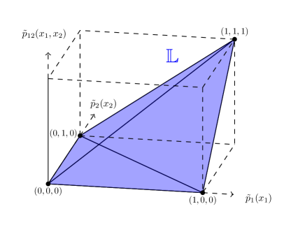
Figure 1: Local polytope $\mathbb{L}$ as the linearly constrained domain of the Bethe free energy $\mathcal{F}_{B}$ (simplified illustration on a single-edge graph and two nodes $X_{1},X_{2}$).

2.3 Related Free Energy Approximations

As the Bethe approximation can fail in certain models, various attempts were made to construct alternative types of free energy approximations. In this work we consider the so-called pairwise approximations, which are generalizations of the Bethe free energy that preserve two of its favorable properties: first, they include statistics that are defined over at most two variables; second, they are defined on the local polytope $\mathbb{L}$ and thus bounded by a relatively small number of linear constraints. This enables an efficient optimization of the objective function by methods of constrained numerical optimization and using its minima to estimate the partition function and marginals. Among all pairwise approximations we focus on two specific classes: those which make a different entropy approximation than $\mathcal{F}_{B}$ but leave the average energy $\mathbb{E}_{\tilde{p}_{i},\tilde{p}_{ij}}[E(\bm{x})]$ unchanged (Sec. 2.3.1); and those which keep the Bethe entropy (8) but modify the energy $E(\bm{x})$ in (2) or, in other words, the model parameters $J_{ij}$, $\theta_{i}$ (Sec. 2.3.2).

2.3.1 Generalizing the Bethe Entropy

While the Gibbs free energy (6) is convex on its domain, this is not guaranteed for the Bethe free energy; in fact, $\mathcal{F}_{B}$ is convex on $\mathbb{L}$ if and only if the graph contains at most one loop [Heskes, 2004, Watanabe and Fukumizu, 2009]. This is because the Bethe entropy $\mathcal{S}_{{B}}$ is generally not concave which has sometimes been considered the reason why the Bethe approximation fails in loopy graphs [Wainwright et al., 2005, Heskes, 2006]. Hence, alternative approximations use a provably convex entropy approximation and are thus convex on $\mathbb{L}$.

Let $\bm{c}\coloneqq\{c_{ij},c_{i}\,|\,(i,j)\in\mathbf{E},i\in\mathbf{X}\}$ be a set of counting numbers with one pairwise number $c_{ij}$ for each edge and one local number $c_{i}$ for each node. We define an $\mathcal{F}_{\bm{c}}$ - approximation to the Gibbs free energy as

$$\mathcal{F}_{\bm{c}}=\mathbb{E}_{\tilde{p}_{i},\tilde{p}_{ij}}[E(\bm{x})]-\tilde{\mathcal{S}}_{\bm{c}}$$ (12)

with the average energy unmodified as in (9) and a generalized entropy approximation of the form

$$\tilde{\mathcal{S}}_{\bm{c}}=\sum_{(i,j)\in\mathbf{E}}c_{ij}\mathcal{S}_{ij}+\sum_{i\in\mathbf{X}}\,c_{i}\mathcal{S}_{i}.$$ (13)

Note that, for $c_{ij}=1$ and $c_{i}=1-d_{i}$ we reobtain the Bethe entropy (8). The generalization (13) creates additional freedom in choosing the entropy approximation by weighting the pairwise and local entropies differently than in the Bethe approximation. A result of Heskes [2006] says that $\tilde{\mathcal{S}}_{\bm{c}}$ is convex if, for all $i\in\mathbf{X}$ and $(i,j)\in\mathbf{E}$, there exist auxiliary numbers $\tilde{c}_{(i,j)},\tilde{c}_{(i,j)\rightarrow i},\tilde{c}_{i}\geq 0$ such that

$$\begin{split}\textasciiacute c_{ij}&\,=\,\tilde{c}_{(i,j)}+\sum\limits_{j\in\mathcal{N}(i)}\tilde{c}_{(i,j)\rightarrow i}\\ c_{i}&\,=\,\tilde{c}_{i}-\tilde{c}_{(i,j)\rightarrow i}-\tilde{c}_{(i,j)\rightarrow j}\end{split}$$ (14)

for all $c_{ij},c_{i}\in\bm{c}$. We briefly introduce two particular approximations $\mathcal{F}_{\bm{c}}$ that satisfy the properties in (14) (i.e., that are convex on $\mathbb{L}$) and that we will compare to other methods in our experiments in Sec. 4.

Tree-Reweighted Free Energies.

The tree-reweighted free energies (TRW) use a weighted sum of entropies over spanning trees in the graph, and are not only convex but also provide an upper bound to the log-partition function [Wainwright et al., 2005]. One chooses a set $\mathcal{T}$ of spanning trees $T$ and a valid tree distribution $\rho(T)$ over all $T\in\mathcal{T}$. The pairwise counting numbers $c_{ij}$ are then computed as edge occurrence probabilities representing the proportions how often an edge occurs in the tree set $\mathcal{T}$, weighted by $\rho(T)$. More precisely, we set $c_{ij}=\sum\limits_{T\in\mathcal{T}}\rho(T)\,I_{(i,j)}(T)$, where $I_{(i,j)}$ indicates if an edge $(i,j)$ is contained in a tree $T$ or not. The local counting numbers are then set to $c_{i}=1-\sum\limits_{j\in\mathcal{N}(i)}c_{ij}$. This ensures that the entropy of each node is in sum counted precisely once and hence the entropy approximation is exact on tree graphs. Further details (including the choice of spanning trees) are provided in Kolmogorov and Wainwright [2006], Jancsary and Matz [2011].

Least-Squares-Convex Free Energies.

The intuition behind Least-Squares (LS) Convex Free Energies proposed by Hazan and Shashua [2008] is to keep $\mathcal{F}_{\bm{c}}$ as close to the Bethe free energy as possible, but with counting numbers $\bm{c}$ that satisfy the convexity conditions (14). Specifically, one solves the LS program

$$\min\sum\limits_{(i,j\in\mathbf{E})}\big{(}\tilde{c}_{(i,j)}+\tilde{c}_{(i,j)\rightarrow i}+\tilde{c}_{(i,j)\rightarrow j}-1\big{)}^{2}$$ (15)

where the minimization is performed with respect to all nonnegative auxiliary numbers
$\tilde{c}_{i},\tilde{c}_{(i,j)},\tilde{c}_{(i,j)\rightarrow i},\tilde{c}_{(i,j)\rightarrow j}$ (for all $i\in\mathbf{X},(i,j)\in\mathbf{E}$) satisfying the linear constraints

$$\tilde{c}_{i}+\sum\limits_{j\in\mathcal{N}(i)}(\tilde{c}_{(i,j)}+\tilde{c}_{(i,j)\rightarrow j})=1,\quad i\in\mathbf{X}.$$ (16)

Afterwards, one computes $c_{ij}$ and $c_{i}$ according to (14). Other ways to set the counting numbers were, e.g., proposed by Wiegerinck and Heskes [2002], Globerson and Jaakkola [2007b], Meshi et al. [2009]. These approaches are mostly inferior to the above methods.

2.3.2 Changing the State Energy

The approximations $\mathcal{F}_{\bm{c}}$ introduced in Sec. 2.3.1 share the favorable property that the average energy is computed as in the Gibbs free energy (6) (but extended to $\mathbb{L}$, which may still alter the location of the minimum). Recently, an alternative class of approximations were proposed that leave the entropy approximation as in the Bethe free energy but modify the state energy (2) by scaling the model parameters. This may seem unintuitive as now both aspects of the approximation – the average energy and the entropy – are incorrect. However, some experimental results show improvements over the Bethe approximation [Knoll et al., 2023].

Let $\bm{\zeta}\coloneqq\{\zeta_{ij},\zeta_{i}\,|\,(i,j)\in\mathbf{E},i\in\mathbf{X}\}$ be a set of scale factors with one pairwise scale factor $\zeta_{ij}$ for each edge and one local scale factor $\zeta_{i}$ for each node. We define an $\mathcal{F}_{\bm{\zeta}}$ - approximation to the Gibbs free energy as

$$\mathcal{F}_{\bm{\zeta}}=\mathbb{E}_{\tilde{p}_{i},\tilde{p}_{ij}}[\tilde{E}_{\bm{\zeta}}(\bm{x})]-\mathcal{S}_{{B}}$$ (17)

with a $\bm{\zeta}$-scaled state energy of the form

$$\tilde{E}_{\bm{\zeta}}(\bm{x})=-\!\!\sum\limits_{(i,j)\in\mathbf{E}}\!\!(\zeta_{ij}J_{ij})x_{i}x_{j}-\sum\limits_{i\in\mathbf{X}}(\zeta_{i}\theta_{i})x_{i}$$ (18)

and the Bethe entropy $\mathcal{S}_{{B}}$ from (8). If all factors $\zeta_{ij},\zeta_{i}$ are set to one we reobtain the Bethe approximation.

The idea behind this approach is as follows: Strong correlations between variables (represented by high values of $|J_{ij}|$) can have a detrimental influence on the accuracy of the Bethe approximation [Weller et al., 2014, Knoll and Pernkopf, 2019]. By decreasing $|J_{ij}|$, the approximation becomes more reliable – however, with respect to a different model. Still, the error induced by $\mathcal{F}_{\bm{\zeta}}$ with respect to the approximated model is often smaller than the error induced by $\mathcal{F}_{B}$ with respect to the original model. In Leisenberger et al. [2024], this behavior has been explained by the fact that $\mathcal{F}_{\bm{\zeta}}$ becomes convex on a submanifold of $\mathbb{L}$ if the correlations are sufficiently weakened. There are only few attempts in the literature following this approach. Here we introduce one of them, that we will later use as comparison method in our experiments (Sec. 4).

Self-Guided Belief Propagation.

Self-Guided Belief Propagation (SBP) exploits the well known relationship between the Bethe approximation and the popular loopy belief propagation (LBP) algorithm. It starts with a completely uncorrelated model (i.e., where all $J_{ij}$ are set zo zero) and successively increases the correlations $J_{ij}$ until LBP, which is sequentially applied during this procedure, either fails to converge for some intermediate state of the model or converges to a fixed point of the original model. In our context, this means that we successively increase a pairwise scale factor $\zeta_{ij}=\zeta$ (that is the same for all edges) starting from $\zeta=0$ and setting the local scale factors $\zeta_{i}$ to one (i.e., leaving the local potentials $\theta_{i}$ unmodified), until LBP either fails to find the minimum of $\mathcal{F}_{\bm{\zeta}}$ for some $\zeta\in(0,1)$ or finds the minimum of $\mathcal{F}_{B}$ for $\zeta=1$. It uses the minimum of $\mathcal{F}_{\bm{\zeta}}$ (or $\mathcal{F}_{B}$) associated to the final state of convergence of LBP to estimate the marginals and partition function. The detailed algorithm is described in [Knoll et al., 2023].

Another approximation of the class $\mathcal{F}_{\bm{\zeta}}$ successively deletes edges from the model; this corresponds to setting pairwise scale factors $\zeta_{ij}$ associated to deleted edges to zero [Leisenberger et al., 2022]. However, SBP proves to be the more flexible algorithm.

2.4 Other Related Work

Higher-Order Variational Inference.

Increasing the complexity of variational inference can help to achieve a higher accuracy. The exact solution can be computed by the junction-tree algorithm whose complexity increases exponentially with the size of the largest clique in the graph [Lauritzen and Spiegelhalter, 1988]. Methods that make higher order entropy approximations were constructed by Yedidia et al. [2005]. Other methods whose efficiency is located ’between’ pairwise approximations and exact inference include join graph propagation [Dechter et al., 2002], loop corrections [Mooij et al., 2007], oriented trees [Globerson and Jaakkola, 2007a], and variable clamping [Weller and Jebara, 2014b].

Message Passing Algorithms.

Having its origins in statistical mechanics [Bethe, 1935, Peierls, 1936], the Bethe approximation has gained popularity in the computer science and statistics community when Yedidia et al. [2001] have proven its connection to loopy belief propagation. Inspired by their discovery, other researchers designed alternative free energies that are related to similar message passing algorithms [Yedidia et al., 2005, Hazan and Shashua, 2008, Meltzer et al., 2009]. These are often efficient but can fail to converge to a fixed point. Also, the convergence behavior of LBP has been subject of research [Tatikonda, 2003, Ihler et al., 2005, Mooij and Kappen, 2007, Leisenberger et al., 2021].

Minimizing Free Energy Approximations.

In practice, it can be difficult to minimize a certain type of free energy approximation, in particular if it is non-convex and has multiple local minima. Various methods were proposed: gradient-based algorithms combined with projection steps [Welling and Teh, 2001, Shin, 2012]; a double-loop algorithm that applies a concave-convex decomposition [Yuille, 2002]; combinatorial optimization [Weller and Jebara, 2014a]; convex optimization [Weller et al., 2014]; and projected Quasi-Newton methods [Schmidt et al., 2009, Jancsary and Matz, 2011, Leisenberger et al., 2024].

3 ADAPTIVE FREE ENERGY APPROXIMATIONS

In this section we analyze the two classes of pairwise free energy approximations $\mathcal{F}_{\bm{c}}$ and $\mathcal{F}_{\bm{\zeta}}$ introduced in Sec. 2.3.1 and Sec. 2.3.2 in a broader context. Our goal is to identify regimes of the counting numbers $\bm{c}$ and scale factors $\bm{\zeta}$ that are related to accurate approximations $\mathcal{F}_{\bm{c}}$ and $\mathcal{F}_{\bm{\zeta}}$. For that purpose, we vary these parameters systematically in appropriate intervals and, for each realization of $\bm{c}$ and $\bm{\zeta}$, evaluate the approximation accuracy induced by $\mathcal{F}_{\bm{c}}$ and $\mathcal{F}_{\bm{\zeta}}$; that is, we compare the minima of $\mathcal{F}_{\bm{c}}$ and $\mathcal{F}_{\bm{\zeta}}$ to the exact marginals and partition function which were computed with the junction tree algorithm [Lauritzen and Spiegelhalter, 1988]. For minimizing free energy approximations of class $\mathcal{F}_{\bm{c}}$ or $\mathcal{F}_{\bm{\zeta}}$, we use techniques of constrained numerical optimization [Nocedal and Wright, 2006]. In particular, we apply a projected Quasi-Newton algorithm which iteratively performs second-order parameter updates, by using an approximation to the inverse Hessian. To ensure that the iterates stay within the local polytope $\mathbb{L}$, a projection step is required. The algorithm stops when it reaches a stationary point (usually a minimum) of the free energy approximation. All details including pseudocode are contained in the Appendix (Alg. 1, named F-MIN).

For error evaluation, we measure three kinds of errors: the $\ell^{1}$-errors between exact and approximate singleton and pairwise marginals, and the absolute error between the exact and approximate log-partition function. In addition to the error evaluation and analysis, another aspect is of practical importance: do algorithms like Bethe, TRW, LS-Convex, and SBP capture favorable regimes of $\bm{c}$ and $\bm{\zeta}$ well, or do there exist optimal settings of $\bm{c}$ or $\bm{\zeta}$ that are not related to any of the ’existing’ free energy approximations? We address this question by comparing the governing parameters $\bm{c}$ and $\bm{\zeta}$ associated to the baseline algorithms to optimal settings of $\bm{c}$ and $\bm{\zeta}$ (i.e., with minimum errors).

In this section we consider a complete graph on $10$ nodes that allows for tractable exact inference. Further evaluations on different graphs exhibit a similar behavior and are shown in the Appendix. We analyze both attractive and mixed models (Sec. 2.1). For either type, we consider two different scenarios regarding the pairwise potentials $J_{ij}$: weak correlations with all $J_{ij}$ being uniformly sampled from $(0,0.5)$ resp. $(-0.5,0.5)$, and strong correlations with all $J_{ij}$ being uniformly sampled from $(0,2)$ resp. $(-2,2)$. We consider three different scenarios regarding the local potentials $\theta_{i}$ that are uniformly sampled from $(-0.2,0.2)$, $(-0.6,0.6)$, or $(-1,1)$. For each configuration of the potentials, the results (i.e., the errors and the estimated values of $\bm{c}$ and $\bm{\zeta}$ shown as vertical lines in Fig. 2, Fig. 3) are averaged over $100$ individual models.

3.1 Analysis of Class $\mathcal{F}_{\bm{c}}$-Approximations

To simplify our considerations, we focus on a specific subclass of $\mathcal{F}_{\bm{c}}$ where the pairwise entropies in (13) share the same counting number, i.e., $c_{ij}=c$ for all edges. In Meshi et al. [2009] it has been argued that free energies of class $\mathcal{F}_{\bm{c}}$ should be variable-valid, i.e., that the entropy approximation is exact on a tree. This can be achieved by setting the local counting numbers

$$c_{i}=1-\sum\limits_{j\in\mathcal{N}(i)}c_{ij}$$ (19)

for all nodes. Then the local counting numbers are implicitly parameterized via $c$ too. For error evaluation, we vary $c$ in the interval $(0,3)$. Note that $c=1$ corresponds to the Bethe free energy $\mathcal{F}_{B}$.

The first row in Fig. 2 shows the results for attractive models. The estimates for singleton and pairwise marginals are improved if $c$ decreases. Especially the least-squares (LS) convex energy (Sec. 2.3.1) finds a good regime for the counting numbers, as is shown by the orange vertical line, and outperforms the Bethe approximation (represented by the black vertical line); however, this advantage shrinks if $J_{ij}$ increases. The estimates of the log-partition function are less sensitive to changes in the counting numbers, unless they become too small. In this regard, the LS-convex free energy appears not to be a decent choice and is inferior to Bethe. However, there appears to be an optimal regime of $c$ that is located between $\mathcal{F}_{B}$ and the LS-convex energy. Note that the counting numbers of TRW are often similar to those of LS-convex, and not explicitly shown in this analyses.

The second row in Fig. 2 shows the results for mixed models. If $J_{ij}$ is small, $\mathcal{F}_{B}$ finds almost optimal estimates for all quantities; however, its accuracy degrades if pairwise potentials become stronger in which case a minimum error is achieved if $c$ grows beyond one. Beyond a certain threshold (which also depends on the strength of the local potentials $\theta_{i}$) the marginal error increases again, while the error in the log-partition function keeps relatively stable at a low level. The red, green, and blue line (adapted to $\theta_{i}$) represent the counting numbers $c$ as estimated by our algorithm ADAPT-$c$ that will be introduced in Sec. 3.3. As ADAPT-$c$ also takes the local potentials into account, three different vertical lines are shown. While, for small $J_{ij}$, the estimated $c$ is almost identical to the pairwise Bethe counting number (i.e., $c=1$), estimates of $c$ made by ADAPT-$c$ usually increase if $J_{ij}$ increases. This has a beneficial effect on the partition function (for all settings of $\theta_{i}$) and the pairwise marginals (for stronger $\theta_{i}$) when estimated by ADAPT-$c$.

3.2 Analysis of Class $\mathcal{F}_{\bm{\zeta}}$-Approximations

Again we facilitate our analysis by only modifying the pairwise potentials $J_{ij}$, while setting the local scale factors $\zeta_{i}$ in (18) to one for all nodes (i.e., we leave the local potentials $\theta_{i}$ unchanged). We further assume that all edges share the same pairwise scale factor, i.e., $\zeta_{ij}=\zeta$. This enables us to directly compare our results to self-guided belief propagation (SBP, Sec. 2.3.2) which makes the same assumptions. For error evaluation, we vary $\zeta$ in the interval $(0,1.5)$.

The first row in Fig. 3 shows the results for attractive models. We observe that the singleton and pairwise marginal error develops similarly as for class $\mathcal{F}_{\bm{c}}$; in particular, Bethe fails to approximate the marginals if $J_{ij}$ is large, while improvements can be made if $\zeta$ is decreased to a certain level. Same as the Bethe approximation, SBP mostly uses a scale factor of $\zeta=1$ in attractive models. Our algorithm ADAPT-$\zeta$ (introduced in Sec. 3.3) aims to reduce $\zeta$ and affect a ’smoothening’ of $\mathcal{F}_{B}$ until it gets a relatively convex shape. This approach has a positive effect on estimating singleton marginals, while an optimal $\zeta$ for estimating pairwise marginals tends to be underestimated. Moreover, $\mathcal{F}_{\bm{\zeta}}$-approximations (except for $\mathcal{F}_{B}$) do generally entail unstable estimates of the partition function and should be used with care for that purpose. As ADAPT-$\zeta$ takes the local potentials into account, three lines represent the associated estimates of $\zeta$ (red, green, and blue).

The second row in Fig. 3 shows the results for general models. Usually, $\mathcal{F}_{B}$ outperforms other $\mathcal{F}_{\bm{\zeta}}$ - approximations if $J_{ij}$ is small (in which case it is equivalent to SBP). If $J_{ij}$ increases, the scale factor $\zeta$ should be decreased to a certain optimal level that depends on the local potentials $\theta_{i}$. For all quantities of interest, SBP makes clear improvements over $\mathcal{F}_{B}$ in mixed models (drawn by the red, green, and blue line adapted to $\theta_{i}$). However, there is some more room for further improvement over SBP regarding the choice of an optimal $\zeta$ (particularly for strong pairwise potentials $J_{ij}$).

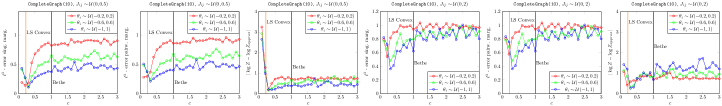
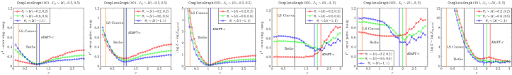
Figure 2: Approximation behavior of $\mathcal{F}_{\bm{c}}$. First row: attractive models; second row: mixed models.

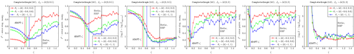
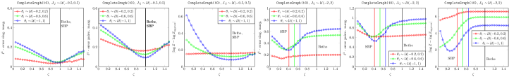
Figure 3: Approximation behavior of $\mathcal{F}_{\bm{\zeta}}$. First row: attractive models; second row: mixed models.

3.3 Adaptive $\mathcal{F}_{\bm{c}}$ - and $\mathcal{F}_{\bm{\zeta}}$ - approximations

This subsection includes a conceptional description of our two algorithms ADAPT-$c$ and ADAPT-$\zeta$ that we propose and evaluate in this work. Detailed pseudocodes are contained in the Appendix (Algorithms 3 and 4).

3.4 Attractive Models: ADAPT-$\zeta$

For attractive models, we propose an adaptive algorithm of class $\mathcal{F}_{\bm{\zeta}}$, named ADAPT-$\zeta$. In these models, the Bethe approximation regularly fails to approximate the quantities of interest; in particular, the estimated marginals are often highly inaccurate if the pairwise potentials are strong. This behavior has been explained by the non-convexity of the Bethe entropy (and thus the Bethe free energy) and is shared by other free energy approximations that are not provably convex [Wainwright et al., 2008, Weller et al., 2014, Leisenberger et al., 2024]. More precisely, the Bethe entropy develops multiple minima which ’pushes’ the minima of $\mathcal{F}_{B}$ towards extreme values of the pseudomarginals. This effect is related to the ’overcounting’ of information and thus overconfidence caused by loopy belief propagation in graphs with multiple cycles [Weiss, 2000, Ihler et al., 2005].

Our algorithm ADAPT-$\zeta$ aims to compensate for this unwanted behavior by using a ’close-to-convex’ version of $\mathcal{F}_{B}$ within the class $\mathcal{F}_{\bm{\zeta}}$. More precisely, it continuously modifies the Bethe free energy by reducing the pairwise potentials $J_{ij}$ in small steps (or, in other words, the joint pairwise scale factor $\zeta$, starting from $\zeta=1$) until $\mathcal{F}_{\bm{\zeta}}$ becomes convex or all except one minimum disappears (which we interpret as ’close-to-convexity’). Formally, it searches for the largest $\zeta$ such that $\mathcal{F}_{\bm{\zeta}}$ has a unique minimum, i.e.,

$$\begin{split}&\zeta^{\ast}=\,\max\limits_{(0,1]}\,\zeta,\\ &\text{s.t.}\,\,\,\mathcal{F}_{\bm{\zeta}}\,\,\,\text{has a unique minimum.}\end{split}$$ (20)

Note that we cannot solve problem (20) exactly as there does not exist a practicable result that is equivalent to uniqueness of a minimum. Thus, to verify that $\mathcal{F}_{\bm{\zeta}}$ has a unique minimum, we use a sufficient condition of Mooij and Kappen [2007] which is based on the spectral radius of the LBP Jacobian (i.e., we usually end up with a lower bound on $\zeta^{\ast}$). After termination, ADAPT-$\zeta$ requires a single application of F-MIN (Alg. 1 in Appendix B) to minimize the associated free energy approximation $\mathcal{F}_{\bm{\zeta}}$.

3.4.1 Mixed Models: ADAPT-$c$

For mixed models, we propose an adaptive algorithm of class $\mathcal{F}_{\bm{c}}$, named ADAPT-$c$, whose design is motivated by the analyses from Sec. 3.1. In Fig. 2 (second row) we have observed that especially the partition function but also the marginals estimated by $\mathcal{F}_{\bm{c}}$ become more accurate if $c$ increases beyond one; in particular, there appears to be a certain regime of $c$ in which all errors roughly attain a minimum (with the marginal errors increasing again beyond that point). Note that most existing algorithms of class $\mathcal{F}_{\bm{c}}$ such as TRW or LS-convex use counting numbers that are smaller than one to make the free energy approximation convex; however, convexity is sometimes not considered a favorable property in mixed models [Weller et al., 2014].

The idea of ADAPT-$c$ is to estimate the threshold of $c$ beyond which only small changes in the partition function error occur. The associated free energy approximation $\mathcal{F}_{\bm{c}}$ will then also be used to estimate the marginals. Let $\Delta c$ be an incremental change in $c$ and let $c_{tol}$ be some value that defines to what extent changes in the estimated log-partition function (i.e., $-\min\mathcal{F}_{\bm{c}}$) are tolerable if $c$ is increased by $\Delta c$. Then we are formally interested in the solution of the following optimization problem:

$$\begin{split}&c^{\ast}=\,\min\limits_{[1,\infty)}\,c,\\ &\text{s.t.}\,\,\,|\min\,\mathcal{F}_{c+\Delta c}\,-\,\min\,\mathcal{F}_{c}\,|\,<\,c_{tol}\end{split}$$ (21)

Note that the solution of (21) depends on the choice of $\Delta c$ and $c_{tol}$. Also, there is no theroretical guarantee on the existence of $c^{\ast}$ for any choice of these two parameters; however, we expect that the existence of a real-valued solution becomes more likely if $c_{tol}$ increases (while $\Delta c$ is kept at a constant level). Thus, ADAPT-$c$ successively increases $c$ in small steps (starting from one, i.e., from the Bethe approximation), and minimizes the associated free energy approximation $\mathcal{F}_{\bm{c}}$ until there are no significant changes in the estimated log-partition function anymore. For each realization of $c$, algorithm F-MIN is applied to find a minimum of $\mathcal{F}_{\bm{c}}$. Fortunately, F-MIN usually converges quickly for most mixed models. Although this procedure is not guaranteed to converge to the solution $c^{\ast}$ of (21), we show in our experiments (Sec. 4) that the results produced by ADAPT-$c$ are fairly promising.

4 EXPERIMENTS

In this section we evaluate and compare the algorithms that were discussed in this work. This includes the Bethe approximation ($\mathcal{F}_{B}$), the tree-reweighted (TRW) free energies, the least-squares-convex (LS-convex) free energies, self-guided belief propagation (SBP), and the two adaptive algorithms ADAPT-$\zeta$ (for attractive models) and ADAPT-$c$ (for mixed models) introduced and explained in Sec. 3. Our experimental setup is similar as in Sec. 3; however, we now vary the size $\hat{J}$ of the intervals $(0,\hat{J})$ (for attractive models) resp. $(-\hat{J},\hat{J})$ (for mixed models) for sampling $J_{ij}$ between $0$ and $3$ in steps of $0.1$ (instead of varying the counting numbers $c$ or scale factors $\zeta$). We compare the performance of the algorithms by using the $\ell^{1}$-errors w.r.t. the singleton and pairwise marginals, and the absolute error w.r.t. the log-partition function. We consider the same scenarios regarding the strength of the local potentials: $\theta_{i}\sim\mathcal{U}(-0.2,0.2)$, $\sim\mathcal{U}(-0.6,0.6)$, and $\sim\mathcal{U}(-1,1)$. The experiments are performed on a complete graph on 10 vertices. Further experiments on grid graphs and Erdos-Renyi random graphs are presented in the Appendix. For each configuration of the potentials and each algorithm the results are averaged over $100$ models.

4.1 Attractive Models

The results for attractive models are shown in Fig. 4. We observe that all algorithms perform well if the correlations between model variables are weak (i.e., if the parameters $J_{ij}$ are small). If $J_{ij}$ increases beyond a certain threshold (that differs for each method), most algorithms experience a significant degradation of their approximation accuracy. This effect is sometimes referred to as a phase transition in the model, and may be explained by the loss of certain properties such as convexity or uniqueness of a minimum [Mooij and Kappen, 2007, Zdeborová and Krzakala, 2016, Leisenberger et al., 2024]. In Wainwright et al. [2008] it is argued that convex approximations are more robust to such spontaneous changes in the model dynamics. For the marginals this agrees with our observations, but for the partition function this is less obvious.

For estimating singleton marginals, ADAPT-$\zeta$ proves to be the most stable alternative that only suffers a slight loss of accuracy during the increase of $J_{ij}$. This is especially distinct for weak local potentials $\theta_{i}$, while for stronger local potentials also SBP improves its performance considerably. For estimating pairwise marginals, ADAPT-$\zeta$ is less robust and slightly outperformed by SBP. For strong local and pairwise potentials, both methods are superior to the convex approximations. For estimating the partition function, SBP clearly shows the most accurate and stable performance while ADAPT-$\zeta$ is not competitive (thus the corresponding results are omitted at this point).

4.2 Mixed Models

The results for mixed models are shown in Fig. 5. Similar as for attractive models, the performance of most algorithms deteriorates if $J_{ij}$ increases. However, this degradation happens rather slowly and steadily than spontanously; in particular, an acceptable approximation accuracy for the marginals is achieved for even higher values of $J_{ij}$. Two possible explanations for this behavior are the following: either properties such as convexity or uniqueness of a minimum are less relevant in mixed models [Weller et al., 2014]; or these properties are relevant but preserved in models with stronger correlations [Leisenberger et al., 2024].

For estimating singleton marginals SBP is the most stable alternative, while ADAPT-$c$ is inferior for weak local potentials $\theta_{i}$. If $\theta_{i}$ increases, ADAPT-$c$ achieves a similar performance as SBP. For pairwise potentials the situation is similiar with ADAPT-$c$ even having a slight advantage over SBP if local potentials are strong. For estimating the partition function, ADAPT-$c$ is by far the most powerful alternative. While any other method fails to approximate $Z$ by several orders of magnitude, ADAPT-$c$ proves to be accurate and stable. These observations are in agreement with the discussion of $\mathcal{F}_{\bm{c}}$-approximations in Sec. 3.1. This indicates that ADAPT-$c$ performs well in approximating the solution of problem (21).

5 CONCLUSION

In this work we have considered pairwise free energy approximations of two particular classes $\mathcal{F}_{\bm{c}}$ and $\mathcal{F}_{\bm{\zeta}}$, which both generalize the Bethe free energy. We have analyzed them in a broader context, by systematically varying their governing parameters (the counting numbers $c_{ij}$ for $\mathcal{F}_{\bm{c}}$ and the scale factors $\zeta_{ij}$ for $\mathcal{F}_{\bm{\zeta}}$) and evaluating the impact on their approximation accuracy. We have drawn practical conclusions, and proposed two adaptive free energy approximations – one for attractive and one for mixed models – that automatically adapt to a model. Our experiments show that our algorithms slightly improve on estimating singleton marginals in attractive models and pairwise marginals in mixed models, and drastically improve on estimating the partition function in mixed models.

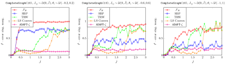
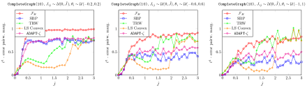
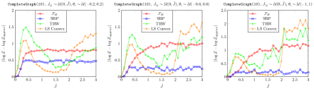
Figure 4: Algorithms Bethe ($\mathcal{F}_{B}$), SBP, TRW, LS-Convex, and ADAPT-$c$’compared on attractive models. First row: $l^{1}$- error on singleton marginals; second row: $l^{1}$- error on pairwise marginals; third row: absolute error on log-partition function.

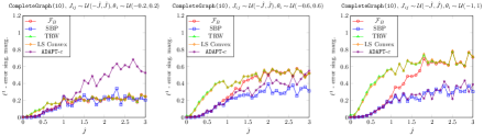
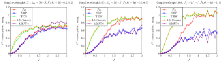
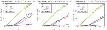
Figure 5: Algorithms Bethe ($\mathcal{F}_{B}$), SBP, TRW, LS-Convex, and ADAPT-$c$ compared on mixed models. First row: $l^{1}$- error on singleton marginals; second row: $l^{1}$- error on pairwise marginals; third row: absolute error on log-partition function.

Appendix A Results from related work

For implementing our algorithms, we require a few results from related work. First, we use from Welling and Teh [2001] that we can reparameterize the local polytope $\mathbb{L}$ to get a simpler description of pairwise free energy approximations (Sec. 2 in the main paper).

Let $X_{i},X_{j}$ be any pair of connected variables and let $\tilde{p}_{i},\tilde{p}_{j},\tilde{p}_{ij}$ be a set of associated pseudo-marginal vectors from the local polytope $\mathbb{L}$ (i.e., with all entries satisfying the constraints in the definition of $\mathbb{L}$). Let us denote the individual pseudo-marginal probabilities for $X_{i}$ and $X_{j}$ being in state $+1$ by $q_{i}\coloneqq\tilde{p}_{i}(X_{i}=+1)$ and $q_{j}\coloneqq\tilde{p}_{j}(X_{j}=+1)$ and let us further denote the joint pseudo-marginal probability for $X_{i},X_{j}$ being both in state $+1$ by $\xi_{ij}\coloneqq\tilde{p}_{ij}(X_{i}=+1,X_{j}=+1)$. Then, as $\tilde{p}_{i},\tilde{p}_{j},\tilde{p}_{ij}$ must satisfy the constraints of $\mathbb{L}$, all five remaining entries of these vectors can already be expressed in terms of $q_{i},q_{j},\xi_{ij}$ according to the following table:

Table 1: Joint probability table of two binary variables $X_{i}$ and $X_{j}$.

$\tilde{p}_{ij}(X_{i},X_{j})$	$X_{j}=+1$	$X_{j}=-1$
$X_{i}=+1$	$\xi_{ij}$	$q_{i}-\xi_{ij}$	$q_{i}$
$X_{i}=-1$	$q_{j}-\xi_{ij}$	$1+\xi_{ij}-q_{i}-q_{j}$	$1-q_{i}$
	$q_{j}$	$1-q_{j}$

Additionally, we have constraints on the independent parameters $q_{i},q_{j},\xi_{ij}$ of the form

$$0< \,\,q_{i}<1,$$

$$0< \,\,q_{j}<1,$$

$$\max(0,q_{i}+q_{j}-1)< \,\,\xi_{ij}<\min(q_{i},q_{j}).$$

This step reparameterizes the local polytope by exploiting probabilistic dependencies between variables and removing a considerable number of redundant parameters. If we collect all node-specific variables $q_{i}$ in a vector $\bm{q}$ and all edge-specific parameters $\xi_{ij}$ in a vector $\bm{\xi}$, we can compactly rewrite the local polytope $\mathbb{L}$ as the set

$$\begin{split}\hskip-14.22636pt\mathbb{L}=\{&(\bm{q};\bm{\xi})\in\mathbb{R}^{\lvert\mathbf{X}\rvert+\lvert\mathbf{E}\rvert}:0<q_{i}<1,i\in\mathbf{X};\\ &\max(0,q_{i}+q_{j}-1)<\xi_{ij}<\min(q_{i},q_{j}),(i,j)\in\mathbf{E}\}.\end{split}$$ (22)

This reparameterization of $\mathbb{L}$ also reparameterizes the Bethe free energy: By substituting the expressions from Table 1 into the statistics of $\mathcal{F}_{B}$, it takes the simpler form

$$\begin{split}\mathcal{F}_{B}(\bm{q};\bm{\xi})=&-\sum_{(i,j)\in\mathbf{E}}\,(1+2\;(2\,\xi_{ij}-q_{i}-q_{j}))\,J_{ij}+\,\,\sum_{i\in\mathbf{X}}(1-2q_{i})\,\theta_{i}\\ &-\Big{(}\sum_{(i,j)\in\mathbf{E}}\mathcal{S}_{ij}\;-\;\sum_{i\in\mathbf{X}}(d_{i}-1)\,\mathcal{S}_{i}\Big{)},\end{split}$$ (23)

with the pairwise entropies

$$\begin{split}\hskip-4.26773pt\mathcal{S}_{ij}=&-\xi_{ij}\log\xi_{ij}-(1+\xi_{ij}-q_{i}-q_{j})\log(1+\xi_{ij}-q_{i}-q_{j})\\ &-(q_{i}-\xi_{ij})\log(q_{i}-\xi_{ij})-(q_{j}-\xi_{ij})\log(q_{j}-\xi_{ij})\end{split}$$ (24)

and the local entropies

$$\begin{split}\mathcal{S}_{i}=-q_{i}\log q_{i}-(1-q_{i})\log(1-q_{i}).\end{split}$$ (25)

By introducing counting numbers and/or scale factors as in Sec. 2.3 of the main paper, it is straightforward to adapt this reparameterization steps to free energy approximations of class $\mathcal{F}_{\bm{c}}$ or $\mathcal{F}_{\bm{\zeta}}$. Next, we show that we can directly parameterize pairwise free energy approximations via the singleton pseudo-marginals [Welling and Teh, 2001, Weller, 2015]. Without loss of generality, we assume that we modify the counting numbers $c_{ij},c_{i}$ and $\zeta_{ij},\zeta_{i}$ at the same time, i.e., obtain a combination $\mathcal{F}_{\bm{c},\bm{\zeta}}$ of class $\mathcal{F}_{\bm{c}}$ and $\mathcal{F}_{\bm{\zeta}}$. Then, by differentiating $\mathcal{F}_{\bm{c},\bm{\zeta}}$ with respect to $\xi_{ij}$ and setting the derivative to zero, one obtains a quadratic equation in $q_{i},q_{j},\xi_{ij}$ whose unique solution is given by

$$\begin{split}&\xi_{ij}^{\ast}(q_{i},q_{j})=\frac{1}{2\alpha_{ij}}\Big{(}Q_{ij}-\sqrt[\ ]{Q_{ij}^{2}-4\alpha_{ij}(1+\alpha_{ij})q_{i}q_{j}}\,\,\Big{)},\\ &\text{where}\,\,\quad\alpha_{ij}=e^{4\frac{\zeta_{ij}J_{ij}}{c_{ij}}}-1\quad\,\,\text{and}\quad\,\,Q_{ij}=1+\alpha_{ij}(q_{i}+q_{j}).\end{split}$$ (26)

In other words, for any $\bm{q}$ there exists at most one $\bm{\xi}^{\ast}(\bm{q})$ (defined in (26)) such that $\big{(}\bm{q};\bm{\xi}^{\ast}(\bm{q})\big{)}$ can be a minimum of $\mathcal{F}_{\bm{c},\bm{\zeta}}$. As a consequence, all minima of $\mathcal{F}_{\bm{c},\bm{\zeta}}$ must lie on a $\lvert\mathbf{X}\rvert$- dimensional submanifold $\mathbb{B}$ of $\mathbb{L}$ that we define as

$$\begin{split}\mathbb{B}\coloneqq\{&(\bm{q};\bm{\xi}^{\ast}(\bm{q}))\in\mathbb{L}:\,\,0<q_{i}<1,i\in\mathbf{X};\\ &\,\,\xi_{ij}^{\ast}(q_{i},q_{j})\,\,\,\text{given by}\,\,\,\eqref{eq:xi_optimal},\,(i,j)\in\mathbf{E}\}.\end{split}$$ (27)

Finally, we require the gradient of free energy approximations of class $\mathcal{F}_{\bm{c}}$ and $\mathcal{F}_{\bm{\zeta}}$ [Weller, 2015]. Again, we assume without loss of generality that we modify the counting numbers $c_{ij},c_{i}$ and $\zeta_{ij},\zeta_{i}$ at the same time, i.e., obtain a combination $\mathcal{F}_{\bm{c},\bm{\zeta}}$ of class $\mathcal{F}_{\bm{c}}$ and $\mathcal{F}_{\bm{\zeta}}$. Then the first-order partial derivatives of $\mathcal{F}_{\bm{c},\bm{\zeta}}$ on $\mathbb{B}$ are

$$\begin{split}\frac{\partial}{\partial q_{i}}\mathcal{F}_{\bm{c},\bm{\zeta}}=-2\,(\zeta_{i}\theta_{i})+2\sum\limits_{j\in\mathcal{N}(i)}(\zeta_{ij}J_{ij})+\log\Big{(}\frac{q_{i}^{c_{i}}}{(1-q_{i})^{c_{i}}}\prod\limits_{j\in\mathcal{N}(i)}\frac{(q_{i}-\xi_{ij}^{\ast})^{c_{ij}}}{(1+\xi_{ij}^{\ast}-q_{i}-q_{j})^{c_{ij}}}\Big{)}.\end{split}$$ (28)

Appendix B Details on Algorithms

This section includes the pseudocodes of the algorithms that we have proposed and applied in our work:

• Algorithm 1 F-MIN was used in Sec. 3 and 4 of the main paper to minimize an arbitrary pairwise free energy approximation of class $\mathcal{F}_{\bm{c}}$ or $\mathcal{F}_{\bm{\zeta}}$ (or a combination of both) to obtain estimates to the exact marginals and partition function.

• Algorithm 2 is used as a subroutine in F-MIN for an adaptive choice of the step size in the projected Quasi-Newton iterations.

• Algorithm 3 is ADAPT-$c$ which was proposed in the main paper for approximate inference in mixed models.

• Algorithm 4 is ADAPT-$\zeta$ which was proposed in the main paper for approximate inference in attractive models.

Algorithm 1 describes our proposed method F-MIN for minimizing a free energy approximation $\mathcal{F}_{\bm{c},\bm{\zeta}}$ of class $\mathcal{F}_{\bm{c}}$ or $\mathcal{F}_{\bm{\zeta}}$ (or a combination of both) on $\mathbb{B}$ that we have applied in our experiments in Sec. 3 and 4 in the main paper. First, one initializes the singleton pseudomarginals $\bm{q}^{(0)}$. Until convergence, F-MIN iterates through the following steps: Update of the search direction according a quasi-Newton scheme, i.e., with the inverse Hessian being replaced by an approximation; projecting the largest possible step back into $\mathbb{B}$; optimizing the step size via an adaptive Wolfe line search (WOLFE-LS, described in Algorithm 2); updating the parameter vector according to

$$\bm{q}^{(t+1)}=\bm{q}^{(t)}-\rho^{(t)}\cdot(\textbf{B}^{(t)})^{T}\,\nabla\mathcal{F}_{\bm{c},\bm{\zeta}}(\bm{q}^{(t)}),$$ (29)

and updating the current approximation to the inverse Hessian (we use the BFGS update rules for approximating the inverse Hessian, Nocedal and Wright [2006]). For checking convergence, we compute the gradient norm with respect to the current parameter vector $\bm{q}^{(t)}$. After F-MIN has converged, it returns a stationary point $\bm{q}^{\ast}$ (usually a minimum) of $\mathcal{F}_{\bm{c},\bm{\zeta}}$.

A free energy approximation $\mathcal{F}_{\bm{c},\bm{\zeta}}$ of class $\mathcal{F}_{\bm{c}}$ or $\mathcal{F}_{\bm{\zeta}}$ (or their combination)

Stationary point $\bm{q}^{\ast}$ of $\mathcal{F}_{\bm{c},\bm{\zeta}}$

Initialize $\bm{q}^{(0)}$ randomly in $\mathbb{B}$ $\triangleright$ Initialization of singleton pseudo-marginals

Initialize estimate of singleton marginals $\bm{q}^{(t)}\leftarrow\bm{q}^{(0)}$

Initialize $\textbf{B}^{(t)}$ randomly as a matrix of size $|\mathbf{X}|\times|\mathbf{X}|$

while $\lVert\nabla\mathcal{F}_{\bm{c},\bm{\zeta}}\big{(}\bm{q}^{(t)}\big{)}\rVert>\epsilon$ do $\triangleright$ Check for convergence

  $\bm{q}^{\text{old}}\leftarrow\bm{q}^{(t)}$ $\triangleright$ Store current parameter vector

  $\bm{d}^{(t)}\leftarrow-\big{(}\textbf{B}^{(t)}\big{)}^{T}\,\nabla\mathcal{F}_{\bm{c},\bm{\zeta}}\big{(}\bm{q}^{(t)}\big{)}$ $\triangleright$ Update search direction

  $\bm{q}^{\pi}\leftarrow\bm{q}^{(t)}+\bm{d}^{(t)}$

  while $\bm{q}^{\pi}\notin\mathbb{B}$ do $\triangleright$ Project $\bm{q}^{\pi}$ back into $\mathbb{B}$

   $\rho^{\max}\leftarrow 0.9\cdot\rho^{\max}$

   $\bm{q}^{\pi}\leftarrow\bm{q}^{(t)}+\rho^{\max}\cdot\bm{d}^{(t)}$

  end while

  $\rho^{(t)}\leftarrow\texttt{WOLFE-LS}(\bm{q}^{(t)},\bm{q}^{\pi})$ $\triangleright$ Compute step size via Algorithm 2

  $\bm{q}^{(t)}\leftarrow\bm{q}^{(t)}+\rho^{(t)}\cdot(\bm{q}^{\pi}-\bm{q}^{(t)})$ $\triangleright$ Update parameter vector

  $\bm{s}^{(t)}\leftarrow\bm{q}^{(t)}-\bm{q}^{\text{old}}$

  $\bm{y}^{(t)}\leftarrow\nabla\mathcal{F}_{\bm{c},\bm{\zeta}}\big{(}\bm{q}^{(t)}\big{)}-\nabla\mathcal{F}_{\bm{c},\bm{\zeta}}\big{(}\bm{q}^{\text{old}}\big{)}$ $\triangleright$ BFGS update rules

  $\gamma^{(t)}\leftarrow(\bm{s}^{(t)})^{T}\bm{y}^{(t)}$ $\triangleright$   for approximating

  $\textbf{B}^{(t)}\leftarrow\textbf{B}^{(t)}+\frac{1}{\big{(}\gamma^{(t)}\big{)}^{2}}\big{(}\gamma^{(t)}+(\bm{y}^{(t)})^{T}\textbf{B}^{(t)}\bm{y}^{(t)}\big{)}$ $\triangleright$ the inverse Hessian

       $+\frac{1}{\gamma^{(t)}}\big{(}\textbf{B}^{(t)}\bm{y}^{(t)}(\bm{s}^{(t)})^{T}+\bm{s}^{(t)}(\bm{y}^{(t)})^{T}\textbf{B}^{(t)}\big{)}$

end while

return $\bm{q}^{(t)}$ $\triangleright$ Return a stationary point of the provided free energy approximation

Algorithm 1 F-MIN (Projected Quasi-Newton for minimizing free energy approximations of class $\mathcal{F}_{\bm{c}}$ or $\mathcal{F}_{\bm{\zeta}}$)

The Wolfe conditions used in the adaptive line search stategy are as follows:

$$\hskip-8.5359pt\mathcal{F}_{\bm{c},\bm{\zeta}}\big{(}\bm{q}^{\text{tail}}+\rho^{\text{W}}\cdot(\bm{q}^{\text{head}}-\bm{q}^{\text{tail}})\big{)}\,\leq\,\mathcal{F}_{\bm{c},\bm{\zeta}}\big{(}\bm{q}^{\text{tail}}\big{)}+\tau_{1}\cdot\rho^{\text{W}}\cdot\bm{d}^{T}\,\nabla\mathcal{F}_{\bm{c},\bm{\zeta}}\big{(}\bm{q}^{\text{tail}}\big{)}$$ (W1)

$$\hskip-8.5359pt\bm{d}^{T}\,\nabla\mathcal{F}_{\bm{c},\bm{\zeta}}\big{(}\bm{q}^{\text{tail}}+\rho^{\text{W}}\cdot(\bm{q}^{\text{head}}-\bm{q}^{\text{tail}})\big{)}\,\geq\,\tau_{2}\cdot\bm{d}^{T}\,\nabla\mathcal{F}_{\bm{c},\bm{\zeta}}\big{(}\bm{q}^{\text{tail}}\big{)}$$ (W2)

The parameter vectors $\bm{q}^{\text{tail}}$ and $\bm{q}^{\text{head}}$ specify the search interval. Condition (W1) ensures that there is a sufficient decrease of the energy function after each iteration. This can be achieved by sufficiently reducing the step size $\rho^{\text{W}}$ to prevent $\mathcal{F}_{approx}$ from increasing again (which may happen if the step is too large). Conversely, condition (W2) ensures that we do not stop moving along the search direction $\bm{d}$, as long as the energy function descends sufficiently steeply. Hence, the step size must not be chosen too small. Both conditions together guarantee that the step size is neither chosen too great nor too small. The parameters $\tau_{1}$ and $\tau_{2}$ control how ’strict’ the individual conditions are. Following a recommendation of Nocedal and Wright [2006], we have selected numerical values of $\tau_{1}=10^{-4}$ and $\tau_{2}=0.9$ for our experiments in Sec. 3 and 4 in the main paper. The detailed procedure of computing a step size satisfying the Wolfe conditions is described in Algorithm 2. It is used as subroutine in Algorithm 1.

Endpoints $\bm{q}^{\text{tail}}$, $\bm{q}^{\text{head}}$ of search interval

Step size $\rho^{\text{W}}$ satisfying the Wolfe conditions (W1) and (W2)

$\bm{d}\leftarrow\bm{q}^{\text{head}}-\bm{q}^{\text{tail}}$ $\triangleright$ Search direction

Initialize step size $\rho^{\text{W}}$ randomly between zero and one

while (W1) is satisfied and (W2) is not satisfied do

  $\rho^{\text{W}}=1.1\cdot\rho^{\text{W}}$ $\triangleright$ Expand interval of potential step sizes

end while

if (W1) and (W2) are satisfied then

  return $\rho^{\text{W}}$ $\triangleright$ STOP. Feasible step size has been found

else

  $l\leftarrow 0$ $\triangleright$ Define new search interval for feasible step size

  $r\leftarrow\rho^{\text{W}}$ $\triangleright$ Upper bound of new search interval

  while (W1) or (W2) is not satisfied do $\triangleright$ Contraction phase

   Pick $\rho^{\text{W}}$ randomly from interval $(l,r)$

   if (W1) is not satisfied then

     $r\leftarrow\rho^{\text{W}}$ $\triangleright$ Upper bound of search interval is reduced

   else

     $l\leftarrow\rho^{\text{W}}$ $\triangleright$ Lower bound of search interval is increased

   end if

  end while

end if

return $\rho^{\text{W}}$

Algorithm 2 WOLFE-LS (Adaptive line search with Wolfe conditions)

Next we present pseudocodes on our algorithms ADAPT-$c$ and ADAPT-$\zeta$ that we have explained in Sec. 3 and compared to other algorithms in Sec. 4 of the main paper.

$\mathcal{F}_{B}$ on an undirected graphical model. $\triangleright$ Start with the Bethe approximation

$c\leftarrow 1$ $\triangleright$ Initialize the joint pairwise counting number

$\log{Z_{approx}^{old}}\leftarrow 0$ $\triangleright$ Initialize current estimate of $-\log{Z}$

$\bm{q}^{(t)}\leftarrow\texttt{F-MIN}(\mathcal{F}_{B})$ $\triangleright$ Minimize the current free energy approximation $\mathcal{F}_{B}$ with Algorithm 1

$\log{Z_{approx}}\leftarrow\mathcal{F}_{B}(\bm{q}^{(t)})$ $\triangleright$ Update current estimate of $-\log{Z}$

while $|\log{Z_{approx}}-\log{Z_{approx}^{old}}|<\epsilon_{Z}$ and $c<c_{max}$ do $\triangleright$ $c_{max}$ specifies an upper bound on $c$

  $\log{Z_{approx}^{old}}\leftarrow\log{Z_{approx}}$ $\triangleright$ Update minimum of $\mathcal{F}_{B}$ from previous iteration

  $c+\Delta c$ $\triangleright$ Increase counting number $c$ by some step size $\Delta{c}$

  $\mathcal{F}_{B}\leftarrow\mathcal{F}_{\bm{c}}$ $\triangleright$ Update the free energy approximation based on the current counting number $c$

  $\bm{q}^{(t)}\leftarrow\texttt{F-MIN}(\mathcal{F}_{B})$

  $-\log{Z_{approx}}\leftarrow\mathcal{F}_{B}(\bm{q}^{(t)})$ $\triangleright$ Update current estimate of $-\log{Z}$

end while

return $\bm{q}^{(t)}$

Algorithm 3 Adapt-$c$ (Adaptive algorithm for optimizing a class $\mathcal{F}_{\bm{c}}$-approximation in mixed models.

$\mathcal{F}_{B}$ on an undirected graphical model. $\triangleright$ Start with the Bethe approximation

$\zeta\leftarrow 1$ $\triangleright$ Initialize the joint pairwise scale factor

while $\mathcal{F}_{B}$ has multiple minima and $\zeta>0$ do $\triangleright$ Use Theorem 4 from Mooij and Kappen [2007]

  $\triangleright$ to check if $\mathcal{F}_{B}$ has a unique minimum

  $\zeta-\Delta\zeta$ $\triangleright$ Decrease scale factor $\zeta$ by some step size $\Delta\zeta$

  $\mathcal{F}_{B}\leftarrow\mathcal{F}_{\bm{\zeta}}$ $\triangleright$ Update the free energy approximation based on the current scale factor $\zeta$

end while

$\bm{q}^{(t)}\leftarrow\texttt{F-MIN}(\mathcal{F}_{B})$ $\triangleright$ Minimize the current free energy approximation $\mathcal{F}_{B}$ with Algorithm 1

return $\bm{q}^{(t)}$

Algorithm 4 Adapt-$\zeta$ (Adaptive algorithm for optimizing class $\mathcal{F}_{\bm{\zeta}}$-approximation in attractive models

Appendix C Additional analysis of $\mathcal{F}_{\bm{c}}$ - and $\mathcal{F}_{\bm{\zeta}}$ - approximations

This section includes additional experiments. In Sec. C.1, we perform an analogous analysis of class $\mathcal{F}_{\bm{c}}$ approximations as in Sec. 3.1 of the main paper; in Sec. C.2, we perform an analogous analysis of class $\mathcal{F}_{\bm{\zeta}}$ approximations as in Sec. 3.2 of the main paper. We show some more evaluations on the complete graph on $10$ nodes, and additionally on a grid graph on $5\times 5$ vertices, and Erdos-Renyi random graphs [Erdos and Renyi, 1959] on $25$ nodes and an edge probability of $0.2$ (i.e., the probability that a pair of nodes is connected by an edge). The experimental setup is the same as explained in Sec. 3 of the main paper; in particular, the results are averaged over $100$ individual models for each specific configuration of the potentials.

C.1 Additional evaluation of $\mathcal{F}_{\bm{c}}$ - approximations

Figure 1-2 include analyses on the complete graph (attractive and mixed models). Figure 3-4 include analyses on the grid graph (attractive and mixed models). Figure 5-6 include analyses on the Erdos-Renyi graphs (attractive and mixed models). The results are similar as in the main paper.

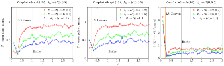
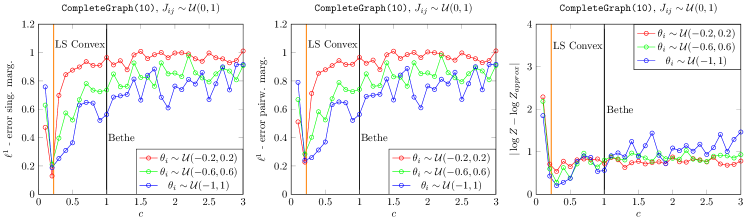
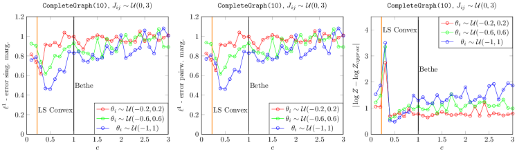
Figure 6: Approximation behavior of $\mathcal{F}_{\bm{c}}$: Attractive models, complete graph on $10$ nodes.

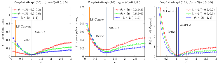
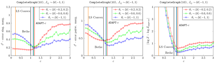
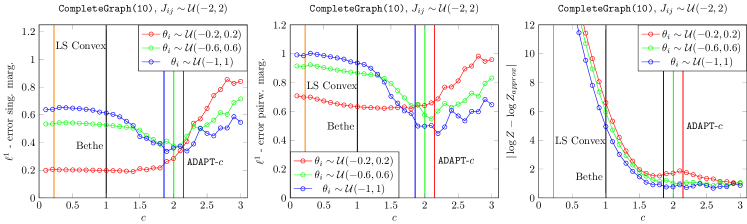
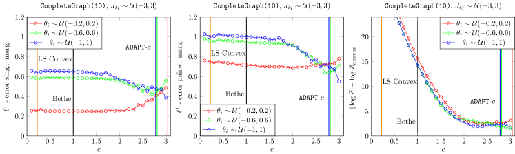
Figure 7: Approximation behavior of $\mathcal{F}_{\bm{c}}$: mixed models, complete graph on $10$ nodes.

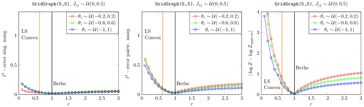
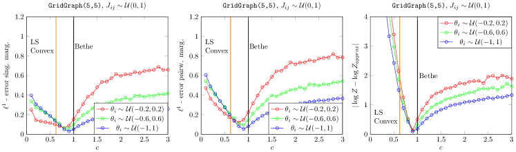
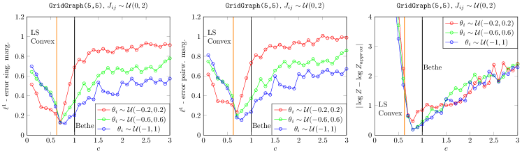
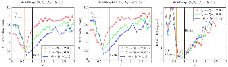
Figure 8: Approximation behavior of $\mathcal{F}_{\bm{c}}$: Attractive models, grid graph $5\times 5$ nodes.

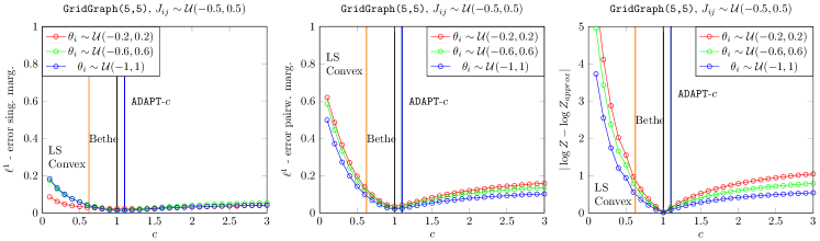
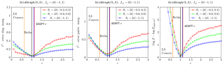
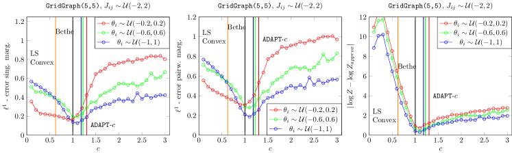
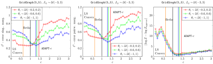
Figure 9: Approximation behavior of $\mathcal{F}_{\bm{c}}$: mixed models, grid graph $5\times 5$ nodes.

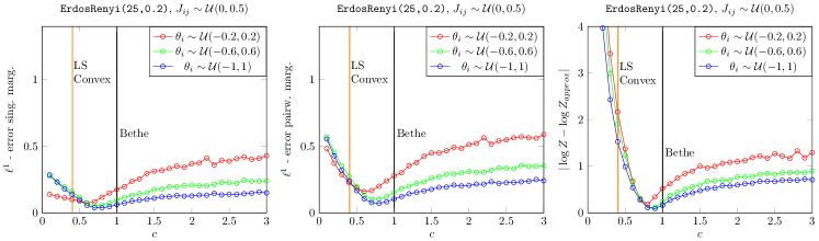
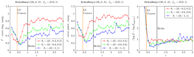
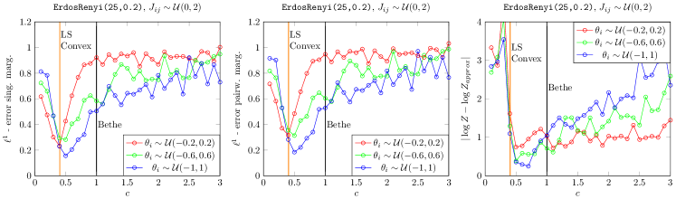
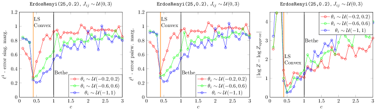
Figure 10: Approximation behavior of $\mathcal{F}_{\bm{c}}$: Attractive models, Erdos-Renyi random graphs on $25$ nodes and an edge probability of $0.2$.

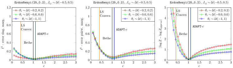
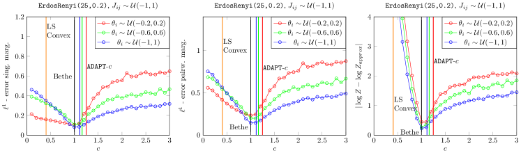
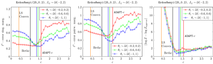
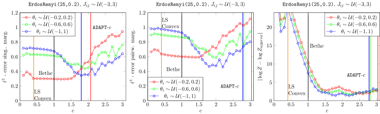
Figure 11: Approximation behavior of $\mathcal{F}_{\bm{c}}$: mixed models, Erdos-Renyi random graphs on $25$ nodes and an edge probability of $0.2$.

C.2 Additional evaluation of class $\mathcal{F}_{\bm{\zeta}}$ approximations

Figure 7-8 include analyses on the complete graph (attractive and mixed models). Figure 9-10 include analyses on the grid graph (attractive and mixed models). Figure 11-12 include analyses on the Erdos-Renyi graphs (attractive and mixed models). The results are similar as in the main paper.

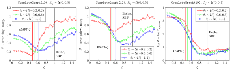
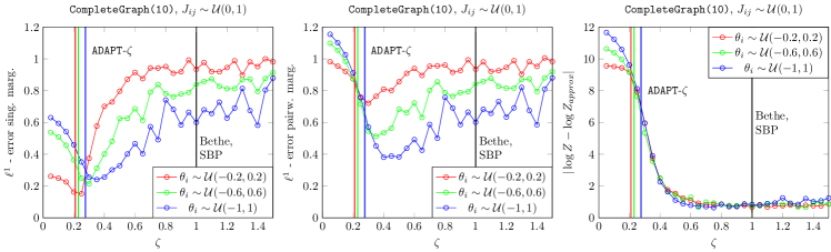
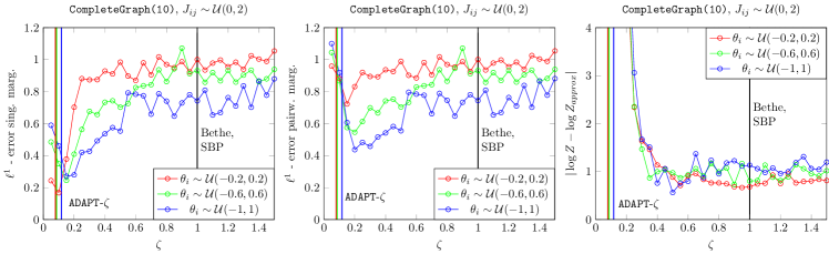
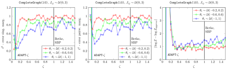
Figure 12: Approximation behavior of $\mathcal{F}_{\bm{\zeta}}$: Attractive models, complete graph on $10$ nodes.

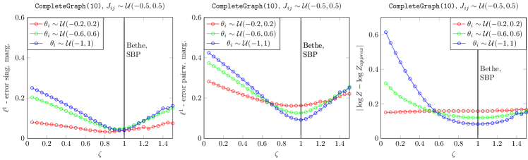
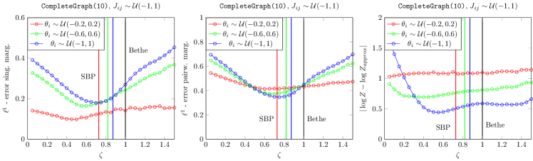
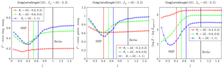
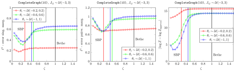
Figure 13: Approximation behavior of $\mathcal{F}_{\bm{\zeta}}$: Mixed models, complete graph on $10$ nodes.

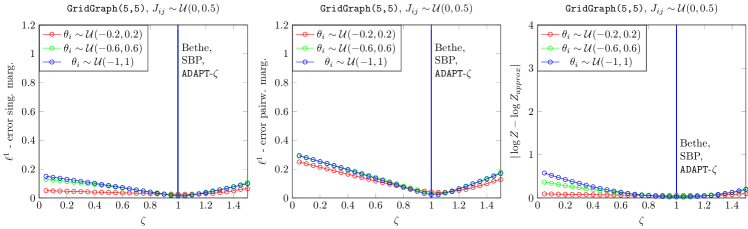
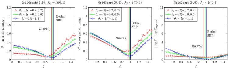
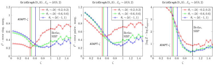
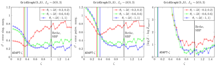
Figure 14: Approximation behavior of $\mathcal{F}_{\bm{\zeta}}$: Attractive models, grid graph $5\times 5$ nodes.

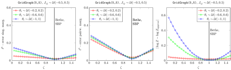
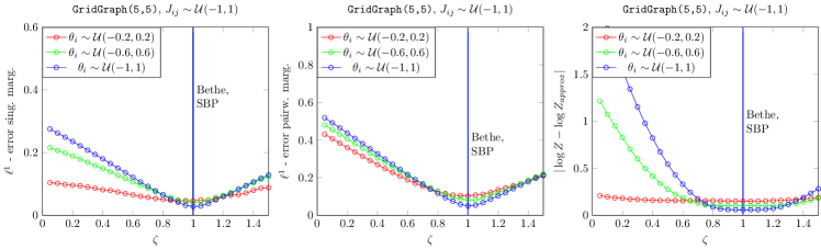
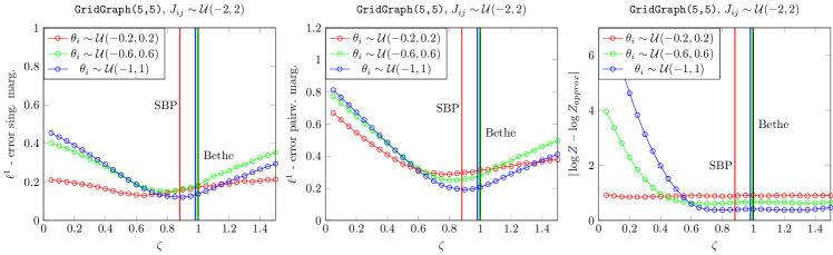
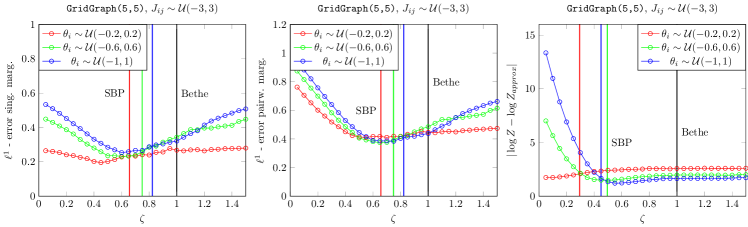
Figure 15: Approximation behavior of $\mathcal{F}_{\bm{\zeta}}$: Mixed models, grid graph $5\times 5$ nodes.

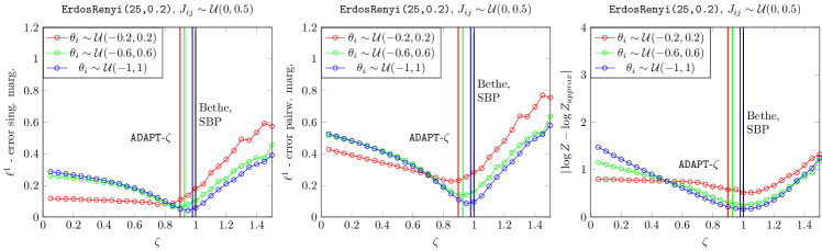
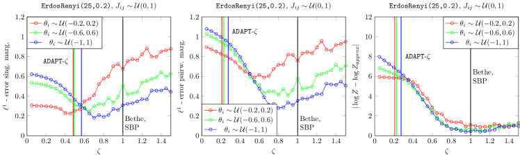
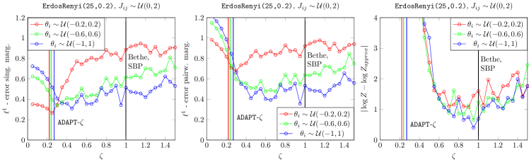
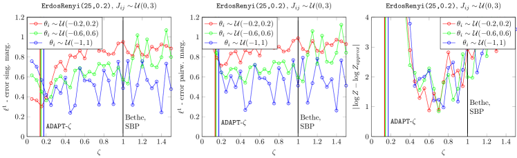
Figure 16: Approximation behavior of $\mathcal{F}_{\bm{\zeta}}$: Attractive models, Erdos-Renyi random graphs on $25$ nodes and an edge probability of $0.2$.

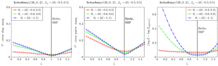
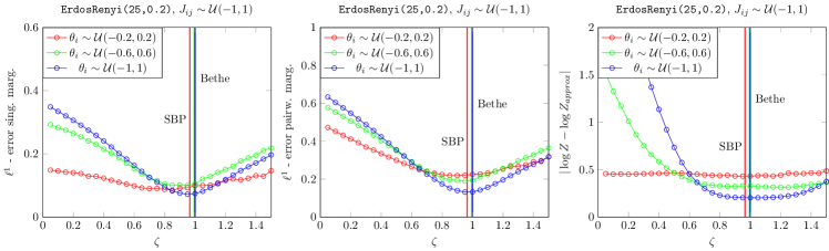
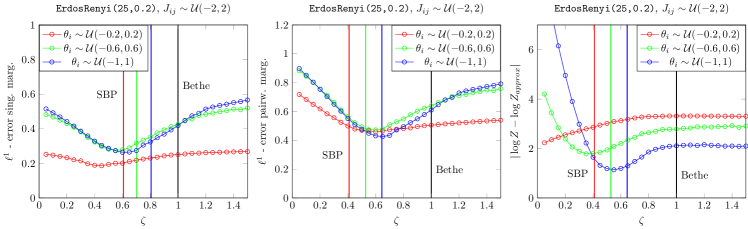
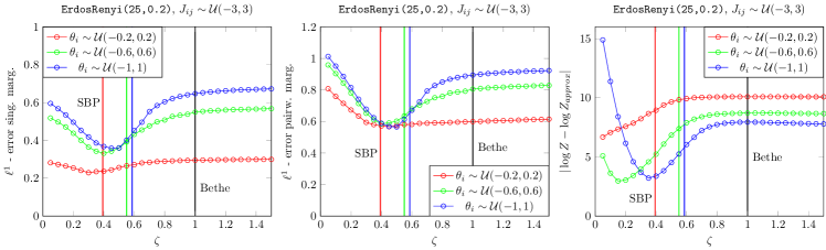
Figure 17: Approximation behavior of $\mathcal{F}_{\bm{\zeta}}$: Mixed models, Erdos-Renyi random graphs on $25$ nodes and an edge probability of $0.2$.

Appendix D Additional experiments

In this section we present additional experiments in which we compare the inference algorithms introduced in the main paper to each other. As in Sec. C of this Appendix, we present additional experiments on the complete graph on $10$ vertices, on a grid graph on $5\times 5$ vertices, and Erdos-Renyi random graphs [Erdos and Renyi, 1959] on $25$ nodes and an edge probability of $0.2$. The experimental setup is the same as in Sec. 4 of the main paper; in particular, in particular, are averaged over $30-100$ individual models for each specific configuration of the potentials. In Sec. D.1 we present results on attractive models, in Sec. D.2 we present results on mixed models.

D.1 Additional experiments for attractive models

In Fig. 13-15 we present additional experiments for attractive models. The results are similar as in the main paper; however, adapt-$\zeta$ loses some of its benefit in the Erdos-Renyi random graphs in which it is slightly outperformed by the LS-Convex free energies.

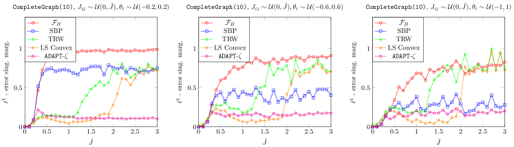
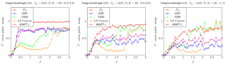
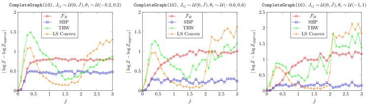
Figure 18: Algorithms Bethe ($\mathcal{F}_{B}$), SBP, TRW, LS-Convex, and ADAPT-$\zeta$ compared on attractive models on a complete graph on $10$ nodes. First row: $l^{1}$- error on singleton marginals; second row: $l^{1}$- error on pairwise marginals; third row: absolute error on log-partition function.

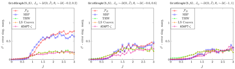
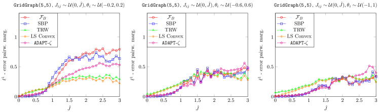
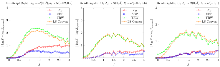
Figure 19: Algorithms Bethe ($\mathcal{F}_{B}$), SBP, TRW, LS-Convex, and ADAPT-$\zeta$ compared on attractive models on a grid graph on $5\times 5$ nodes. First row: $l^{1}$- error on singleton marginals; second row: $l^{1}$- error on pairwise marginals; third row: absolute error on log-partition function.

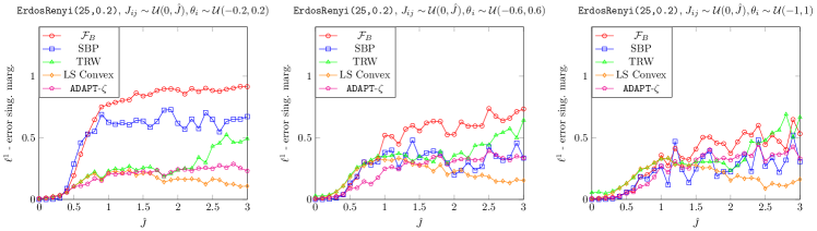
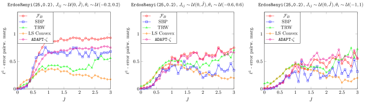
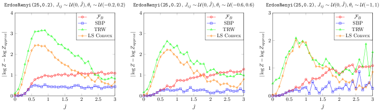
Figure 20: Algorithms Bethe ($\mathcal{F}_{B}$), SBP, TRW, LS-Convex, and ADAPT-$\zeta$ compared on attractive models on Erdos renyi random graphs on $25$ nodes and an edge probability of $0.2$. First row: $l^{1}$- error on singleton marginals; second row: $l^{1}$- error on pairwise marginals; third row: absolute error on log-partition function.

D.2 Additional experiments for mixed models

In Fig. 16-18 we present additional experiments for mixed models. The results are similar as in the main paper; in particular, ADAPT-$c$ is still by far superior to other methods if one aims to estimate the partition function.

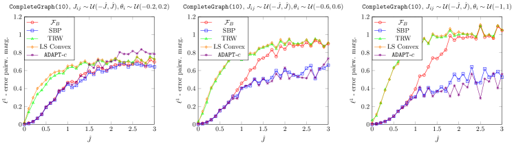
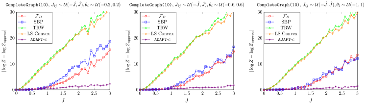
Figure 21: Algorithms Bethe ($\mathcal{F}_{B}$), SBP, TRW, LS-Convex, and ADAPT-$c$ compared on mixed models on a complete graph on $10$ nodes. First row: $l^{1}$- error on singleton marginals; second row: $l^{1}$- error on pairwise marginals; third row: absolute error on log-partition function.

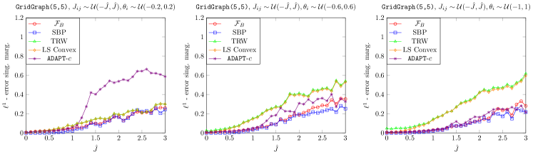
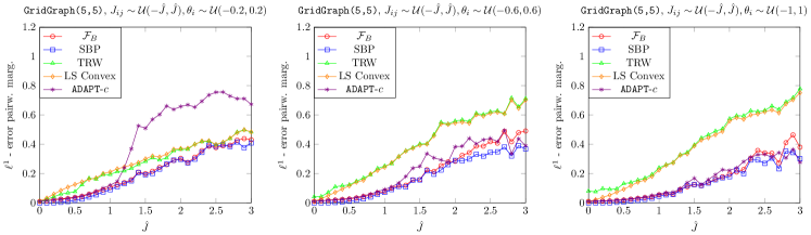
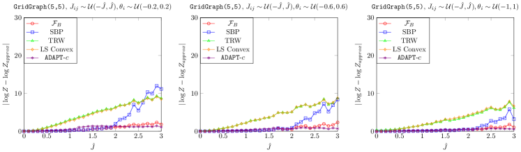
Figure 22: Algorithms Bethe ($\mathcal{F}_{B}$), SBP, TRW, LS-Convex, and ADAPT-$c$ compared on mixed models on a grid graph on $5\times 5$ nodes. First row: $l^{1}$- error on singleton marginals; second row: $l^{1}$- error on pairwise marginals; third row: absolute error on log-partition function.

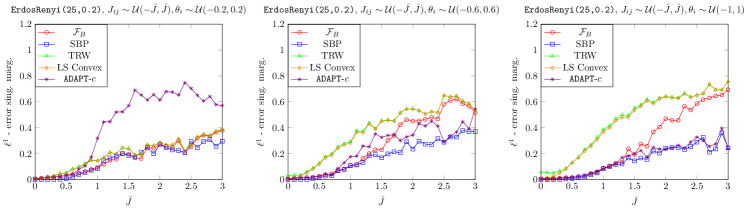
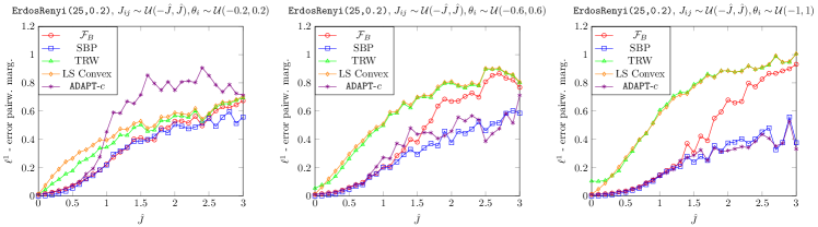
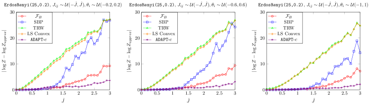
Figure 23: Algorithms Bethe ($\mathcal{F}_{B}$), SBP, TRW, LS-Convex, and ADAPT-$c$ compared on mixed models on Erdos renyi random graphs on $25$ nodes and an edge probability of $0.2$. First row: $l^{1}$- error on singleton marginals; second row: $l^{1}$- error on pairwise marginals; third row: absolute error on log-partition function.

References

- Bethe [1935] Hans A. Bethe. Statistical theory of superlattices. Proceedings of the Royal Society A, 150(871):552–575, 1935.
- Cooper [1990] Gregory F. Cooper. The computational complexity of probabilistic inference using Bayesian belief networks. Artificial intelligence, 42(2-3):393–405, 1990.
- Dagum and Luby [1993] Martin J. Dagum and Michael G. Luby. Approximate probabilistic reasoning in Bayesian belief networks is NP-hard. Artificial Intelligence, 60(1):141–153, 1993.
- Dechter et al. [2002] Rina Dechter, Kalev Kask, and Robert Mateescu. Iterative join-graph propagation. In Proceedings of UAI, 2002.
- Eaton and Ghahramani [2013] Frederik Eaton and Zoubin Ghahramani. Model reductions for inference: generality of pairwise, binary, and planar factor graphs. Neural Computation, 25(5):1213–1260, 2013.
- Erdos and Renyi [1959] Paul Erdos and Alfred Renyi. On random graphs I. Publicationes Mathematicae, 6(3–4):290–297, 1959.
- Globerson and Jaakkola [2007a] Amir Globerson and Tommi Jaakkola. Convergent propagation algorithms via oriented trees. In Proceedings of UAI, 2007a.
- Globerson and Jaakkola [2007b] Amir Globerson and Tommi Jaakkola. Approximate inference using conditional entropy decompositions. In Proceedings of AISTATS, 2007b.
- Hazan and Shashua [2008] Tamir Hazan and Amnon Shashua. Convergent message-passing algorithms for inference over general graphs with convex free energies. In Proceedings of UAI, 2008.
- Heskes [2003] Tom Heskes. Stable fixed points of loopy belief propagation are minima of the Bethe free energy. In Proceedings of NIPS, 2003.
- Heskes [2004] Tom Heskes. On the uniqueness of loopy belief propagation fixed points. Neural Computation, 16(11):2379–2413, 2004.
- Heskes [2006] Tom Heskes. Convexity arguments for efficient minimization of the Bethe and Kikuchi free energies. Journal of Artificial Intelligence Research, 26(1):153–190, 2006.
- Ihler et al. [2005] Alexander T. Ihler, John W. Fisher, and Alan S. Willsky. Loopy belief propagation: convergence and effects of message errors. Journal of Machine Learning Research, 6(1):905–936, 2005.
- Ising [1925] Ernst Ising. Beitrag zur Theorie des Ferromagnetismus. Zeitschrift für Physik, 31(1):253–258, 1925.
- Jancsary and Matz [2011] Jeremy Jancsary and Gerald Matz. Convergent decomposition solvers for tree-reweighted free energies. In Proceedings of AISTATS, 2011.
- Johnson et al. [2016] Jason K. Johnson, Diane Oyen, Michael Chertkov, and Praneeth Netrapalli. Learning planar Ising models. Journal of Machine Learning Research, 17(214):1–26, 2016.
- Jordan et al. [1999] Michael I. Jordan, Zoubin Ghahramani, Tommi S. Jaakkola, and Lawrence K. Saul. An Introduction to Variational Methods for Graphical Models. Machine Learning, 37:183–233, 1999.
- Knoll and Pernkopf [2019] Christian Knoll and Franz Pernkopf. Belief propagation: accurate marginals or accurate partition function – where is the difference? In Proceedings of UAI, 2019.
- Knoll et al. [2023] Christian Knoll, Adrian Weller, and Franz Pernkopf. Self-guided belief propagation – A homotopy continuation method. IEEE Transactions on Pattern Analysis and Machine Intelligence, 45(4):5139–5157, 2023.
- Koller and Friedman [2009] Daphne Koller and Nir Friedman. Probabilistic Graphical Models: Principles and Techniques. MIT press, 2009.
- Kolmogorov and Wainwright [2006] Vladimir Kolmogorov and Martin J. Wainwright. Convergent tree-reweighted message-passing for energy minimization. IEEE Transactions on Pattern Analysis and Machine Intelligence, 28(10):1568–1583, 2006.
- Lauritzen and Spiegelhalter [1988] Steffen L. Lauritzen and David J. Spiegelhalter. Local computations with probabilities on graphical structures and their application to expert systems. Royal Statistical Society, 50(2):157–224, 1988.
- Leisenberger et al. [2021] Harald Leisenberger, Christian Knoll, Richard Seeber, and Franz Pernkopf. Convergence behavior of belief propagation: Estimating regions of attraction via Lyapunov functions. In Proceedings of UAI, 2021.
- Leisenberger et al. [2022] Harald Leisenberger, Franz Pernkopf, and Christian Knoll. Fixing the Bethe approximation: How structural modifications in a graph improve belief propagation. In Proceedings of UAI, 2022.
- Leisenberger et al. [2024] Harald Leisenberger, Christian Knoll, and Franz Pernkopf. On the convexity and reliability of the Bethe free energy approximation. preprint on arxiv:2405.15514, 2024.
- Meltzer et al. [2009] Talya Meltzer, Amir Globerson, and Yair Weiss. Convergent message passing algorithms – a unifying view. In Proceedings of UAI, 2009.
- Meshi et al. [2009] Ofer Meshi, Ariel Jaimovich, Amir Globerson, and Nir Friedman. Convexifying the Bethe free energy. In Proceedings of UAI, 2009.
- Mezard and Montanari [2009] Marc Mezard and Andrea Montanari. Information, Physics, and Computation. Oxford University Press, 2009.
- Mooij et al. [2007] Joris Mooij, Bastian Wemmenhove, Bert Kappen, and Rizzo Tommaso. Loop corrected belief propagation. In Proceedings of AISTATS, 2007.
- Mooij and Kappen [2005] Joris M. Mooij and Hilbert J. Kappen. On the properties of the Bethe approximation and loopy belief propagation on binary networks. Journal of Statistical Mechanics: Theory and Experiment, 2005(11):P11012, 2005.
- Mooij and Kappen [2007] Joris M. Mooij and Hilbert J. Kappen. Sufficient conditions for convergence of the sum–product algorithm. IEEE Transactions on Information Theory, 53(12):4422–4437, 2007.
- Nocedal and Wright [2006] Jorge Nocedal and Stephen J. Wright. Numerical optimization. Springer, 2006.
- Pearl [1988] Judea Pearl. Probabilistic Reasoning in Intelligent Systems: Networks of Plausible Inference. Morgan Kaufmann Publishers, 1988.
- Peierls [1936] Rudolf E. Peierls. Statistical theory of superlattices with unequal concentrations of the components. Proceedings of the Royal Society A, 154(881):207–222, 1936.
- Schmidt et al. [2009] Mark Schmidt, Ewout van den Berg, Michael P. Friedlander, and Kevin Murphy. Optimizing costly functions with simple constraints: A limited-memory projected quasi-newton algorithm. In Proceedings of ICML, 2009.
- Shin [2012] Jinwoo Shin. Complexity of Bethe approximation. In Proceedings of AISTATS, 2012.
- Tatikonda [2003] Sekhar C. Tatikonda. Convergence of the sum-product algorithm. In Proceedings of IEEE Information Theory Workshop, 2003.
- Valiant [1979] Leslie G. Valiant. The complexity of computing the permanent. Theoretical Computer Science, 8(2):189–201, 1979.
- Wainwright et al. [2005] Martin J. Wainwright, Tommi S. Jaakkola, and Alan S. Willsky. A new class of upper bounds on the log partition function. IEEE Transactions on Information Theory, 51(7):2313–2335, 2005.
- Wainwright et al. [2008] Martin J. Wainwright, Michael I. Jordan, et al. Graphical models, exponential families, and variational inference. Foundations and Trends in Machine Learning, 1(1–2):1–305, 2008.
- Watanabe and Fukumizu [2009] Yusuke Watanabe and Kenji Fukumizu. Graph zeta function in the Bethe free energy and loopy belief propagation. In Proceedings of NIPS, 2009.
- Weiss [2000] Yair Weiss. Correctness of local probability propagation in graphical models with loops. Neural Computation, 12(1):1–41, 2000.
- Weller [2015] Adrian Weller. Bethe and related pairwise entropy approximations. In Proceedings of UAI, 2015.
- Weller and Jebara [2014a] Adrian Weller and Tony Jebara. Approximating the Bethe partition function. In Proceedings of UAI, 2014a.
- Weller and Jebara [2014b] Adrian Weller and Tony Jebara. Clamping variables and approximate inference. In Proceedings of NIPS, 2014b.
- Weller et al. [2014] Adrian Weller, Kui Tang, Tony Jebara, and David Sontag. Understanding the Bethe approximation: When and how can it go wrong? In Proceedings of UAI, 2014.
- Welling and Teh [2001] Max Welling and Yee W. Teh. Belief optimization for binary networks: A stable alternative to loopy belief propagation. In Proceedings of UAI, 2001.
- Wiegerinck and Heskes [2002] Wim Wiegerinck and Tom Heskes. Fractional belief propagation. In Proceedings of NIPS, 2002.
- Yedidia et al. [2001] Jonathan S. Yedidia, William T. Freeman, and Yair Weiss. Bethe free energy, Kikuchi approximations, and belief propagation algorithms. In Proceedings of NIPS, 2001.
- Yedidia et al. [2005] Jonathan S. Yedidia, William T. Freeman, and Yair Weiss. Constructing free energy approximations and generalized belief propagation algorithms. IEEE Transactions on Information Theory, 51(7):2282–2312, 2005.
- Yuille [2002] Alan L. Yuille. CCCP algorithms to minimize the Bethe and Kikuchi free energies: Convergent alternatives to belief propagation. Neural Computation, 14(7):1691–1722, 2002.
- Zdeborová and Krzakala [2016] Lenka Zdeborová and Florent Krzakala. Statistical physics of inference: Thresholds and algorithms. Advances in Physics, 65(5):453–552, 2016.