A large momentum transfer atom interferometer without -reversal
Abstract
We present an atom interferometer using large momentum transfer without -reversal. More specifically, we use a microwave /2 pulse to manipulate the spin state of 87Rb atoms before applying a Raman light pulse to achieve 4 momentum transfer per Raman light pulse. A microwave pulse in the middle of the interferometer sequence reverses the spin states, which allows closing of the interferometer arms by the same Raman light pulses without -reversal. We discuss the scalability of this large momentum transfer technique. Our results extend the scope of using large momentum transfer atom optics into atom interferometers where -reversal optics are not available.
Atom interferometers have emerged as pivotal tools in modern physics, enabling high-precision measurements of fundamental constants [1, 2, 3, 4, 5], rigorous tests of physical laws [6, 7, 8, 9], observation of gravitational waves [10, 11, 12], and technological applications such as inertial navigation [13, 14, 15, 16, 17] and gravity mapping [18, 19, 20, 21]. In this paper, we demonstrate a technically simple method to increase the sensitivity of a light pulse atom interferometer using large momentum transfer (LMT).
The operational principle of an atom interferometer involves splitting an atomic wavepacket, allowing it to propagate along two distinct interferometer arms, and subsequently recombining the wavepacket to allow interference. The sensitivity of an atom interferometer increases with the space-time area enclosed by the arms. Increasing the propagation time is one method to increase the sensitivity. Extended propagation times have been achieved through the use of atomic fountains [22, 13, 23], drop towers [24, 25], and micro-g environments [26, 27, 28, 29].
An alternative approach, known as large momentum transfer, increases the momentum imparted to the atomic wavepacket, thus increasing the separation between the interferometer arms. Early realizations of light pulse interferometers, using techniques such as Bragg diffraction [30, 31], Raman transitions [22], and single-photon, long-lived optical transitions [32, 33] typically imparted momentum on the order of to the atomic wavepacket. Since then, more advanced methods have been developed, including adiabatic rapid passage [34, 35, 36], spin-dependent kicks [37], Floquet atom optics [38, 39], Bloch oscillations [5, 40, 41, 42, 43], and higher-order diffraction [44, 45, 7, 46, 47].
These developments have enabled momentum transfers as high as [37, 39, 4]. However, these approaches require either the rapid reversal of the effective wavevector (-reversal [48]) between light pulses or the use of additional lasers, which can be impractical for certain experimental setups [49, 50, 51]. Moreover, implementing the necessary fast switching of the Raman detuning can destabilize the phase of the Raman beams [52]. Furthermore, constraints on size, weight, power, and cost can outweigh the benefits of these techniques, particularly in space-based applications [26, 27].
We present a novel method for performing LMT without the need for -reversal or additional lasers whilst maintaining state selective detection, relying solely on the interaction with an additional microwave field, and demonstrate an implementation. Finally, we propose a pathway for larger momentum transfers for even greater sensitivities.
Our realization of the interferometer scheme uses 87Rb atoms. As shown in Fig. 1(a), we use microwave pulses to directly couple the hyperfine levels of the state, and laser pulses detuned from the state to drive Raman transitions between these levels. Our 4 LMT atom interferometer is realized by three microwave pulses and four Raman pulses, which is illustrated in Fig. 1(b). Our interferometer sequence starts with a spin-dependent-kick (SDK) beam splitter [37]. This SDK beam splitter uses a microwave pulse followed by a Raman pulse to create a momentum separation between two interferometer arms. More specifically, the microwave pulse puts each atom into an equal superposition of two spin states, and , without changing its momentum state. After a period of free evolution, a Raman pulse imparts momenta of to and to , as well as reversing the spin states. After this SDK beam splitter pulse, a second Raman pulse is applied to keep the spatial separation between two interferometer arms at a fixed distance, , where is the temporal separation between the first and second Raman pulses and the atomic mass. The atoms then evolve freely for before the spin states of the two arms are swapped by a microwave pulse. Subsequently there is another free evolution time , following which the two interferometer arms are closed, without -reversal, by applying two more Raman pulses separated by . Finally, after freely evolving for , the two arms are made to interfere by applying the final microwave pulse.
After the above interferometer sequence, the population in , , is determined by
| (1) |
where is the middle point of the interference fringe, is the amplitude of the fringe and and are the phase differences along the two paths due to interactions with the microwave and Raman fields respectively.
We choose to have , so that the interferometer is closed. Then the microwave phase difference is
| (2) |
where is the difference between the microwave frequency and the hyperfine splitting of the state. Further, we choose and so that this
phase is strongly suppressed, even if the microwave detuning is non-zero.
With our symmetric timing, the Raman phase calculated in the short-pulse limit [22, 53] is
| (3) |
where is the constant acceleration of the atom relative to the mirror, projected onto the direction of the Raman beams. The factor originates from the momentum transfer per Raman pulse, and is the interval between the first and the last Raman pulse. The dimensionless factor is a simple way of characterizing the acceleration sensitivity for a given .
In this letter, we study the phase, , defined in Eq. 3, and compare it with that of a standard three-pulse Mach-Zehnder (MZ) atom interferometer. Although our demonstration transfers 4 as shown in Fig. 1(b), the scheme is readily scaled up to transfer 4 without -reversal by the pulse sequence shown in Fig. 1(c).
The apparatus is very similar to that described in Sabulsky et al. [49].
A 3D magneto-optical trap (MOT) of 87Rb atoms is loaded from a -MOT [54]. We apply cooling light near resonant with the transition in addition to repump light near resonant with the transition, using sub-Doppler cooling to reduce the temperature to near 10 K. Optical pumping prepares the atoms into the ground state, distributed across the three sublevels.
During the interferometer sequence, we apply a bias magnetic field of 0.38 G to lift the degeneracy of the states. Our two Raman frequencies and are separated by 6.834 GHz in order to drive the 87Rb hyperfine transition . The Quans laser system which generates this light is described in [49].
Figure 2 shows the preparation of the light for the interferometer. The light at the two Raman frequencies () leaves the output fiber with orthogonal linear polarizations, before passing through a quarter-wave plate (QWP) to become () polarized. After passing through another QWP, is directed to a beam dump by a polarizing beam splitter (PBS) while passes through, reflects off the mirror, passes back through the PBS and the QWP resulting in the polarization , which completes the Raman transition. As is rejected, the Raman transition is not driven [55]. A horn delivers microwave radiation to the atoms through a vacuum window. The microwave source is derived from the Quans Raman laser system, so the radiation is phase-coherent with the beat note between the two Raman beams, as is necessary to form the interferometer. A micro electro-mechanical (MEMS) accelerometer is attached to the rear of the mirror to monitor its acceleration.
As we wish to address only the atoms in the magnetically insensitive state, we apply the following state preparation sequence [51] to further manipulate atoms already prepared into the ground state.
With the intensities of the Raman beams tuned to zero the light shift, we apply a Raman pulse to drive the transition, before applying repumping light to pump the remaining atoms from to . Another Raman pulse transfers the atoms from , leaving the atoms in . We then apply the cooling light to selectively ‘blow away’ the atoms in the state, leaving typically of the initial population, almost all in the state.
The interferometer scheme is shown in Fig. 1(b).
After a microwave pulse places the atoms into a superposition of the two hyperfine states and , the atoms evolve for ms before the sequence of pulses separated by , all of which are 4 ms.
A ms free evolution time follows the final pulse, then the interferometer is closed with a microwave pulse. At the end of this sequence, the fraction of atoms in the state, , is determined by fluorescence detection.
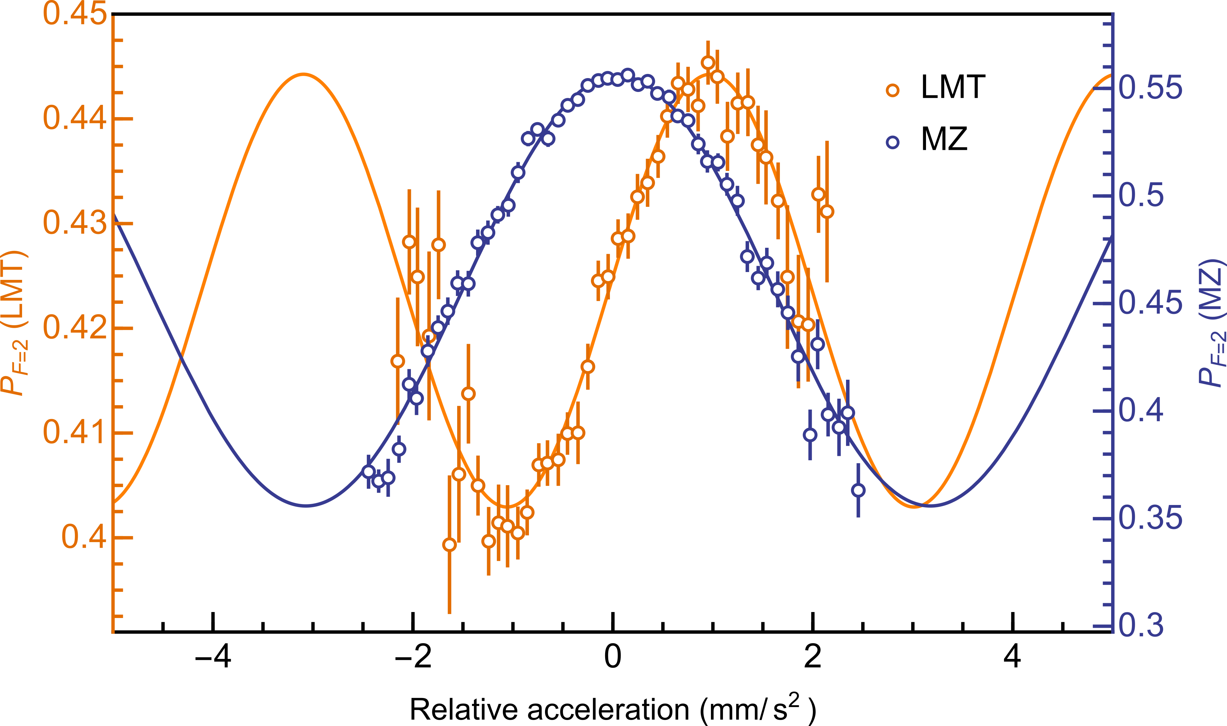
In Fig. 3, we plot as a function of the average mirror acceleration, . This average is taken over the time between the first and last Raman pulses, with a trapezoid weighting, as described in our supplementary material [56]. As a benchmark to compare with our LMT interferometer, we also plot the fringe given by a three-pulse MZ sequence with the same 2T = 16 ms. For the MZ analysis, we use a standard triangular weighting [57] to calculate . We fit each fringe to the function
| (4) |
where is an offset phase. The two fringes have different due to the bias of the MEMS accelerometer. For the MZ interferometer we expect to find because of the momentum transfer per Raman pulse, while for our LMT interferometer scheme we expect , as given by Eq. 3 with . The fits give and , in good agreement with expectations. This shows that our LMT interferometer indeed has a finer fringe spacing by a factor of for the same time . It also verifies that the acceleration weighting function derived in the supplementary material [56] works for the LMT interferometer.
We note that, in the limit of , Eq. 3 gives and the interferometer has no acceleration sensitivity. In this limit, the two paths do not enclose any area and the LMT interferometer becomes a microwave spin-echo sequence. In the limit of , the interferometer reaches its maximum acceleration sensitivity of and the area enclosed is the maximum available with a momentum transfer.
It is instructive to compare the peak-to-peak amplitudes of the two fringes in Fig. 3. The MZ interferometer uses three Raman pulses: , , , and we measured the transfer efficiency of the Raman pulse to be 0.55. As a rough estimate, we can therefore expect a peak-to-peak amplitude of order , and that is close to the 0.2 that we measure. By contrast, the LMT interferometer requires seven pulses: three microwave pulses, for which the population transfer efficiency is , and four Raman pulses. The rough estimate of is close to the measured peak-to-peak amplitude of 0.04.
While in our current setup, we are severely limited by our low pulse efficiencies, these can be greatly improved. In the present apparatus, the microwave field is very inhomogeneous because of standing waves in the chamber, but this can easily be avoided through careful design. The Raman pulse efficiency can be improved, for example, by using the adiabatic-passage technique, as described in [37]. High efficiency will be necessary when our method is extended to larger recoils of because this requires microwave pulses and Raman pulses. With pulse efficiencies of one can expect to have a fringe peak-to-peak amplitude of with a recoil of .
The resulting improvement in sensitivity will be valuable in several applications. Examples include low drift compact accelerometers for navigation [13, 14, 15, 16, 17] or fundamental physics, such as gravitational wave detection using a pair of horizontal accelerometers. [11, 10].
Acknowledgements.
We acknowledge engineering support by J. Dyne and software support by Teodor B Krastev. We thank the UK Science and Technology Research Council (STFC) for funding through grants ST/W006316/1 and ST/V00428X/1.References
- Fixler et al. [2007] J. B. Fixler, G. T. Foster, J. M. McGuirk, and M. A. Kasevich, Atom interferometer measurement of the newtonian constant of gravity, Science 315, 74 (2007).
- Rosi et al. [2014] G. Rosi, F. Sorrentino, L. Cacciapuoti, M. Prevedelli, and G. M. Tino, Precision measurement of the newtonian gravitational constant using cold atoms, Nature (London) 510, 518 (2014).
- Bouchendira et al. [2011] R. Bouchendira, P. Cladé, S. Guellati-Khélifa, F. m. c. Nez, and F. m. c. Biraben, New determination of the fine structure constant and test of the quantum electrodynamics, Phys. Rev. Lett. 106, 080801 (2011).
- Parker et al. [2018] R. H. Parker, C. Yu, W. Zhong, B. Estey, and H. Müller, Measurement of the fine-structure constant as a test of the standard model, Science 360, 191 (2018).
- Morel et al. [2020] L. Morel, Z. Yao, P. Cladé, and S. Guellati-Khélifa, Determination of the fine-structure constant with an accuracy of 81 parts per trillion, Nature (London) 588, 61 (2020).
- Schlippert et al. [2014] D. Schlippert, J. Hartwig, H. Albers, L. L. Richardson, C. Schubert, A. Roura, W. P. Schleich, W. Ertmer, and E. M. Rasel, Quantum test of the universality of free fall, Phys. Rev. Lett. 112, 203002 (2014).
- Zhou et al. [2015] L. Zhou, S. Long, B. Tang, X. Chen, F. Gao, W. Peng, W. Duan, J. Zhong, Z. Xiong, J. Wang, Y. Zhang, and M. Zhan, Test of equivalence principle at level by a dual-species double-diffraction raman atom interferometer, Phys. Rev. Lett. 115, 013004 (2015).
- Zhang et al. [2023] T. Zhang, L.-L. Chen, Y.-B. Shu, W.-J. Xu, Y. Cheng, Q. Luo, Z.-K. Hu, and M.-K. Zhou, Ultrahigh-sensitivity bragg atom gravimeter and its application in testing lorentz violation, Phys. Rev. Appl. 20, 014067 (2023).
- Overstreet et al. [2022] C. Overstreet, P. Asenbaum, J. Curti, M. Kim, and M. A. Kasevich, Observation of a gravitational aharonov-bohm effect, Science 375, 226 (2022).
- Canuel and others [2018] B. Canuel et al., Exploring gravity with the MIGA large scale atom interferometer, Sci. Rep. 8, 14064 (2018).
- Zhan and others [2020] M.-S. Zhan et al., ZAIGA: Zhaoshan long-baseline atom interferometer gravitation antenna, Int. J. Mod. Phys. D 29, 1940005 (2020).
- Badurina and others [2020] L. Badurina et al., AION: an atom interferometer observatory and network, J. Cosmol. Astropart. Phys. 2020 (05), 011.
- Dickerson et al. [2013] S. M. Dickerson, J. M. Hogan, A. Sugarbaker, D. M. S. Johnson, and M. A. Kasevich, Multiaxis inertial sensing with long-time point source atom interferometry, Phys. Rev. Lett. 111, 083001 (2013).
- d’Armagnac de Castanet et al. [2024] Q. d’Armagnac de Castanet, C. Des Cognets, R. Arguel, S. Templier, V. Jarlaud, V. Ménoret, B. Desruelle, P. Bouyer, and B. Battelier, Atom interferometry at arbitrary orientations and rotation rates, Nat. Commun. 15, 6406 (2024).
- Geiger et al. [2011] R. Geiger, V. Ménoret, G. Stern, N. Zahzam, P. Cheinet, B. Battelier, A. Villing, F. Moron, M. Lours, Y. Bidel, et al., Detecting inertial effects with airborne matter-wave interferometry, Nat. Commun. 2, 474 (2011).
- Cheiney et al. [2018] P. Cheiney, L. Fouché, S. Templier, F. Napolitano, B. Battelier, P. Bouyer, and B. Barrett, Navigation-compatible hybrid quantum accelerometer using a kalman filter, Phys. Rev. Appl. 10, 034030 (2018).
- Templier et al. [2022] S. Templier, P. Cheiney, Q. d’Armagnac de Castanet, B. Gouraud, H. Porte, F. Napolitano, P. Bouyer, B. Battelier, and B. Barrett, Tracking the vector acceleration with a hybrid quantum accelerometer triad, Sci. Adv. 8, eadd3854 (2022).
- Stray et al. [2022] B. Stray, A. Lamb, A. Kaushik, J. Vovrosh, A. Rodgers, J. Winch, F. Hayati, D. Boddice, A. Stabrawa, A. Niggebaum, M. Langlois, et al., Quantum sensing for gravity cartography, Nature (London) 602, 590 (2022).
- Li et al. [2023] C.-Y. Li, J.-B. Long, M.-Q. Huang, B. Chen, Y.-M. Yang, X. Jiang, C.-F. Xiang, Z.-L. Ma, D.-Q. He, L.-K. Chen, and S. Chen, Continuous gravity measurement with a portable atom gravimeter, Phys. Rev. A 108, 032811 (2023).
- Ménoret et al. [2018] V. Ménoret, P. Vermeulen, N. Le Moigne, S. Bonvalot, P. Bouyer, A. Landragin, and B. Desruelle, Gravity measurements below 10- 9 g with a transportable absolute quantum gravimeter, Sci. Rep. 8, 12300 (2018).
- Wu et al. [2019] X. Wu, Z. Pagel, B. S. Malek, T. H. Nguyen, F. Zi, D. S. Scheirer, and H. Müller, Gravity surveys using a mobile atom interferometer, Sci. Adv. 5, eaax0800 (2019).
- Kasevich and Chu [1992] M. Kasevich and S. Chu, Measurement of the gravitational acceleration of an atom with a light-pulse atom interferometer, Appl. Phys. B 54, 321 (1992).
- Clairon et al. [1991] A. Clairon, C. Salomon, S. Guellati, and W. D. Phillips, Ramsey resonance in a zacharias fountain, Europhys. Lett. 16, 165 (1991).
- Kulas et al. [2017] S. Kulas, C. Vogt, A. Resch, J. Hartwig, S. Ganske, J. Matthias, D. Schlippert, T. Wendrich, W. Ertmer, E. Maria Rasel, et al., Miniaturized lab system for future cold atom experiments in microgravity, Microgravity Sci. and Technol. 29, 37 (2017).
- Müntinga et al. [2013] H. Müntinga, H. Ahlers, M. Krutzik, A. Wenzlawski, S. Arnold, D. Becker, et al., Interferometry with bose-einstein condensates in microgravity, Phys. Rev. Lett. 110, 093602 (2013).
- Williams et al. [2024] J. R. Williams, C. A. Sackett, H. Ahlers, et al., Pathfinder experiments with atom interferometry in the cold atom lab onboard the international space station, Nat. Commun. 15, 6414 (2024).
- Lachmann et al. [2021] M. D. Lachmann, H. Ahlers, D. Becker, A. N. Dinkelaker, J. Grosse, O. Hellmig, H. Müntinga, V. Schkolnik, S. T. Seidel, T. Wendrich, et al., Ultracold atom interferometry in space, Nat. Commun. 12, 1317 (2021).
- Elsen et al. [2023] M. Elsen, B. Piest, F. Adam, O. Anton, P. Arciszewski, W. Bartosch, D. Becker, K. Bleeke, J. Böhm, S. Boles, et al., A dual-species atom interferometer payload for operation on sounding rockets, Microgravity Sci. and Technol. 35, 48 (2023).
- Barrett et al. [2016] B. Barrett, L. Antoni-Micollier, L. Chichet, B. Battelier, T. Léveque, A. Landragin, and P. Bouyer, Dual matter-wave inertial sensors in weightlessness, Nat. Commun. 7, 13786 (2016).
- Giltner et al. [1995] D. M. Giltner, R. W. McGowan, and S. A. Lee, Theoretical and experimental study of the bragg scattering of atoms from a standing light wave, Phys. Rev. A 52, 3966 (1995).
- Torii et al. [2000] Y. Torii, Y. Suzuki, M. Kozuma, T. Sugiura, T. Kuga, L. Deng, and E. W. Hagley, Mach-zehnder bragg interferometer for a bose-einstein condensate, Phys. Rev. A 61, 041602 (2000).
- Riehle et al. [1991] F. Riehle, T. Kisters, A. Witte, J. Helmcke, and C. J. Bordé, Optical ramsey spectroscopy in a rotating frame: Sagnac effect in a matter-wave interferometer, Phys. Rev. Lett. 67, 177 (1991).
- Hu et al. [2017] L. Hu, N. Poli, L. Salvi, and G. M. Tino, Atom interferometry with the sr optical clock transition, Phys. Rev. Lett. 119, 263601 (2017).
- Kovachy et al. [2012] T. Kovachy, S.-w. Chiow, and M. A. Kasevich, Adiabatic-rapid-passage multiphoton bragg atom optics, Phys. Rev. A 86, 011606 (2012).
- Kotru et al. [2015] K. Kotru, D. L. Butts, J. M. Kinast, and R. E. Stoner, Large-area atom interferometry with frequency-swept raman adiabatic passage, Phys. Rev. Lett. 115, 103001 (2015).
- Chen et al. [2024] X.-L. Chen, S.-B. Lu, C. Sun, M. Jiang, Y. Li, Z.-W. Yao, S.-K. Li, M. Ke, R.-B. Li, J. Wang, and M.-S. Zhan, Robust large-momentum-transfer atom interferometry with raman adiabatic rapid passage, Op. Commun. 573, 131005 (2024).
- Jaffe et al. [2018] M. Jaffe, V. Xu, P. Haslinger, H. Müller, and P. Hamilton, Efficient adiabatic spin-dependent kicks in an atom interferometer, Phys. Rev. Lett. 121, 040402 (2018).
- Rudolph et al. [2020] J. Rudolph, T. Wilkason, M. Nantel, H. Swan, C. M. Holland, Y. Jiang, B. E. Garber, S. P. Carman, and J. M. Hogan, Large momentum transfer clock atom interferometry on the 689 nm intercombination line of strontium, Phys. Rev. Lett. 124, 083604 (2020).
- Wilkason et al. [2022] T. Wilkason, M. Nantel, J. Rudolph, Y. Jiang, B. E. Garber, H. Swan, S. P. Carman, M. Abe, and J. M. Hogan, Atom interferometry with floquet atom optics, Phys. Rev. Lett. 129, 183202 (2022).
- McAlpine et al. [2020] K. E. McAlpine, D. Gochnauer, and S. Gupta, Excited-band bloch oscillations for precision atom interferometry, Phys. Rev. A 101, 023614 (2020).
- Cladé et al. [2009] P. Cladé, S. Guellati-Khélifa, F. m. c. Nez, and F. m. c. Biraben, Large momentum beam splitter using bloch oscillations, Phys. Rev. Lett. 102, 240402 (2009).
- Pagel et al. [2020] Z. Pagel, W. Zhong, R. H. Parker, C. T. Olund, N. Y. Yao, and H. Müller, Symmetric bloch oscillations of matter waves, Phys. Rev. A 102, 053312 (2020).
- Fitzek et al. [2024] F. Fitzek, J.-N. Kirsten-Siemß, E. Rasel, N. Gaaloul, and K. Hammerer, Accurate and efficient bloch-oscillation-enhanced atom interferometry, Phys. Rev. Res. 6, L032028 (2024).
- Lévèque et al. [2009] T. Lévèque, A. Gauguet, F. Michaud, F. Pereira Dos Santos, and A. Landragin, Enhancing the area of a raman atom interferometer using a versatile double-diffraction technique, Phys. Rev. Lett. 103, 080405 (2009).
- Malossi et al. [2010] N. Malossi, Q. Bodart, S. Merlet, T. Lévèque, A. Landragin, and F. P. D. Santos, Double diffraction in an atomic gravimeter, Phys. Rev. A 81, 013617 (2010).
- Zhou et al. [2021] L. Zhou, C. He, S.-T. Yan, X. Chen, D.-F. Gao, W.-T. Duan, Y.-H. Ji, R.-D. Xu, B. Tang, C. Zhou, et al., Joint mass-and-energy test of the equivalence principle at the 10- 10 level using atoms with specified mass and internal energy, Phys. Rev. A 104, 022822 (2021).
- Hartmann et al. [2020] S. Hartmann, J. Jenewein, S. Abend, A. Roura, and E. Giese, Atomic raman scattering: Third-order diffraction in a double geometry, Phys. Rev. A 102, 063326 (2020).
- Durfee et al. [2006] D. S. Durfee, Y. K. Shaham, and M. A. Kasevich, Long-term stability of an area-reversible atom-interferometer sagnac gyroscope, Phys. Rev. Lett. 97, 240801 (2006).
- Sabulsky et al. [2019] D. O. Sabulsky, I. Dutta, E. A. Hinds, B. Elder, C. Burrage, and E. J. Copeland, Experiment to detect dark energy forces using atom interferometry, Phys. Rev. Lett. 123, 061102 (2019).
- Cheng [2020] X. Cheng, Building a Sensitive Atom Interferometer for Navigation, Ph.D. thesis, Imperial College London (2020).
- Peng [2023] G. Peng, A sensitive horizontal atom interferometer for testing acceleration from an in-vacuum source mass, Ph.D. thesis, Imperial College London (2023).
- Lee et al. [2022] J. Lee, R. Ding, J. Christensen, R. R. Rosenthal, A. Ison, D. P. Gillund, D. Bossert, K. H. Fuerschbach, W. Kindel, P. S. Finnegan, et al., A compact cold-atom interferometer with a high data-rate grating magneto-optical trap and a photonic-integrated-circuit-compatible laser system, Nat. Commun. 13, 5131 (2022).
- Hogan et al. [2009] J. M. Hogan, D. M. Johnson, and M. A. Kasevich, Light-pulse atom interferometry, in Atom Optics and Space Physics (IOS Press, 2009) pp. 411–447.
- Dieckmann et al. [1998] K. Dieckmann, R. J. C. Spreeuw, M. Weidemuller, and J. T. M. Walraven, The two-dimensional magneto-optical trap as a source of slow atoms, Physical Review A 58, 3891 (1998).
- [55] When the Raman beams are horizontal, the - and - Raman transitions are degenerate in frequency and have opposite recoil momenta. It is therefore necessary to suppress one of them to avoid splitting the wavefunction at each -pulse. It is not necessary if the beams are vertical because then the Doppler shift removes the frequency degeneracy.
- [56] See Supplemental Material at the end of this document for the derivation of our trapezoidal acceleration weighing function, which includes Refs. [58, 53, 57].
- Barrett et al. [2014] B. Barrett, P.-A. Gominet, E. Cantin, L. Antoni-Micollier, A. Bertoldi, B. Battelier, P. Bouyer, J. Lautier, and A. Landragin, Mobile and remote inertial sensing with atom interferometers, in Atom interferometry (IOS Press, 2014) pp. 493–555.
- Storey and Cohen-Tannoudji [1994] P. Storey and C. Cohen-Tannoudji, The feynman path integral approach to atomic interferometry. a tutorial, Journal de Physique II 4, 1999 (1994).
I Supplemental Material
In an atom interferometer, the probability of detecting atoms in one of two output states is determined by the difference, , in the phases accumulated along the two arms. Our is proportional to the acceleration of the atoms relative to the mirror that retro-reflects the laser light. Vibrations of the mirror are fast enough that the acceleration changes during the interferometer sequence, and therefore we need to consider what kind of average determines . In the case of a standard three-pulse Mach-Zehnder (MZ) interferometer, the acceleration is averaged with a triangular weighting factor [57]. Here we derive the appropriate weighting function for our large momentum transfer (LMT) interferometer and consider how to generalise it to other schemes.
To derive the weighting, we firstly review each of the three phase contributions to the total phase difference, , for our LMT interferometer. We then show the acceleration weighting function of our LMT interferometer is trapezoidal rather than a triangle. Finally, we provide a simple picture to understand the shape of an acceleration weighting function. This picture provides an intuitive way to obtain the acceleration weighting function for an arbitrary pulse sequence, such as a LMT interferometer proposed in Fig. 1c in the main text.
II Phase contributions
Assuming all the atoms are prepared in the F=1 state before the interferometer pulses, then the final population in F=2, , at the output of our interferometer is given by
| (5) |
where is the middle point of the interference fringe, is the amplitude of the fringe and is the total phase difference between two interferometer arms.
Following the formalism and notation in [53], we can calculate this total phase difference, , by separating it into three contributions
| (6) |
where is the difference of the propagation phase between the two interferometer arms, and . We use the same (left/right) notation for the separation phase difference, , and the interaction phase difference, .
We note that for our interferometer, as we have chosen such that for the final pulse the two interferometer arms overlap in space, closing it. Thus, we only need to calculate the sum of and to evaluate .
II.1 Propagation phase
The propagation phase originates from the free-evolution of the wave packet and it is given by
| (7) |
where the sum is over all segments of the left (or right) path, is the classical Lagrangian evaluated at the centre of mass of the wavepacket on the left (or right) trajectory, is the internal atomic energy on that trajectory, and and are the initial time and the final time of each path segment.
In our interferometer, the contribution of is found to be zero. Therefore, is determined by the energy difference of the two internal states, , and the time spent in each internal state, given by
| (8) |
where and are the temporal separations between interferometer pulses shown in Fig. 1b in the main text.
II.2 Interaction phase
The interaction phase comes from the phase of the microwave field or Raman laser imprinted on the wavepacket during a coherent population transfer. The difference in the interaction phases accumulated on the two interferometer arms is given by
| (9) |
where the summation is over all the interaction events, which occur at times and at positions and on the classical trajectories. We will further split the interaction phase out according to whether it arises from a microwave transition or a Raman transition, and respectively. The interaction phase has a () sign when a photon is absorbed(emitted) by an atom.
The microwave phase at an atom’s center of mass position at time is given by
| (10) |
where , and are the frequency, wavevector, and a constant initial phase of the microwave field. We assume the position of the horn is static. Similarly, the Raman phase is given by
| (11) |
where , and are the frequency, wavevector and a constant initial phase of the Raman light. is the frequency difference between the two Raman lasers and has a magnitude of , where is the averaged wavenumber of two Raman lasers of wavelength . The position of the retroreflection mirror can vary in time. Its acceleration is monitored by the MEMS accelerometer.
In our interferometer, the interaction phases accumulated along each arm are given by
| (12) |
where we have labeled each phase contribution with X denoting Raman or MW, denoting pulse number, and the left or right arm. Substituting equations Eq.10 to Eq.12 into Eq.9 gives the interaction phase difference between the two arms of our interferometer:
| (13) |
where we use the averaged classical atom position relative to the mirror, :
| (14) |
II.3 Total phase difference between two arms
The total phase difference between the two interferometer arms can be calculated by substituting Eq.8 and Eq.13 into Eq.6. Noting that we closed the interferometer by choosing , we can separate the microwave and Raman contributions and express as
| (15) |
which is the same form as that of the Eq. 1 in the main text. Then, the microwave phase difference and Raman phase difference are
| (16) |
We assume that in the horizontal direction, the atoms have some constant acceleration , and that the scale of the horizontal trajectories is much less than the microwave wavelength of 4.4 cm. This allows us to ignore the spatially dependent terms of the microwave phase in Eq. 16 to re-write the microwave phase difference between the two arms as:
| (17) |
where is the microwave detuning. This is the derivation of Eq. 2 in the main text.
To derive Eq. 3 we assume a symmetric pulse sequence such that and which simplifies the Raman phase difference to
| (18) |
We have used to show how depends on the separation between the first two Raman pulses, , and the time between the first and the last Raman pulses, . Dividing by makes it simple to compare the acceleration sensitivities of the LMT and MZ interferometers.
III Acceleration weighting function
Phase noise from vibrations has been well-studied [57] in a three-pulse MZ interferometer, where only the laser phase contributes to the total interferometer phase . We apply the same formalism to our LMT interferometer. Although our interaction phase consists of both the Raman laser phase and the microwave phase, only the Raman laser phase is sensitive to the change of the Raman mirror position as shown in Eq.16, and so we will only be considering those pulses when constructing our weighting function. To simplify the discussion we will assume 1D motion of atoms along the direction of the Raman beams.
If we consider an infinitesimal change in the Raman mirror position at time , , we can express the relative positions of the atom, defined in Eq. 14, to be
| (19) |
These changes lead to a change in the total interferometer phase, , which can be written using a time-domain position sensitivity function defined by
| (20) |
Substituting Eq.19 into Eq.15 yields
| (21) |
The vibration-induced phase shift can be calculated
| (22) |
The position sensitivity function can also be regarded as a velocity weighting function.
If we define as with a constraint that , then can be written in terms of a time-dependent acceleration by
| (23) |
where we have used integration by parts and taken . This gives us an acceleration weighting function , which, with the substitutions and , is given by
| (24) |
The weighting function has a trapezoid shape for our LMT interferometer, which is different from a triangular acceleration weighting function for a standard MZ interferometer.
We note that is not normalized. We define a normalization integration to calculate our weighted average acceleration
| (25) |
where is a normalized weighting function of a trapezoid shape. This is how we calculated the time-average acceleration, , in the main text.
IV Geometric explanation for the shape of acceleration weighting functions
In this section, we provide a simpler explanation for the shape of the acceleration weighting function, . This allows us to obtain directly, rather than deriving it from the position sensitivity function.
The change in the total phase difference between the two arms, , only depends on the change of the relative position of atoms referenced to the mirror position. Let us therefore calculate the same , not in the inertial lab frame, but in the non-inertial mirror frame, where the mirror is stationary and the atoms have the additional vibrating motion. In this frame the Lagrangian of an atom, , has an additional term relative to its lab-frame Lagrangian:
| (26) |
where can be understood as a linear potential due to a homogeneous fictitious force . The lab frame Lagrangian is simply given by .
As proved in the path-integral approach to atom interferometry [58], can be treated as a perturbation because its dependence on the spatial coordinates is less than quadratic. Hence the phase shift is obtained by integrating the perturbed Lagrangian, , along the unperturbed path, :
| (27) |
where the unperturbed path, (), of the left (right) interferometer arm is determined by the lab frame Lagrangian, . These unperturbed paths are illustrated in the Fig. 1 (b) in the main text.