[c]U. Wenger
HMC and gradient flow with machine-learned classically perfect fixed-point actions
Abstract
Fixed-point (FP) lattice actions are classically perfect, i.e., they have continuum classical properties unaffected by discretization effects and are expected to have suppressed lattice artifacts at weak coupling. Therefore they provide a possible way to extract continuum physics with coarser lattices, allowing to circumvent problems with critical slowing down and topological freezing towards the continuum limit. We use machine-learning methods to parameterize a FP action for four-dimensional SU(3) gauge theory using lattice gauge-covariant convolutional neural networks. The large operator space allows us to find superior parameterizations compared to previous studies and we show how such actions can be efficiently simulated with the Hybrid Monte Carlo algorithm. Furthermore, we argue that FP lattice actions can be used to define a classically perfect gradient flow without any lattice artifacts at tree level. We present initial results for scaling of the gradient flow with the FP action.
1 Introduction
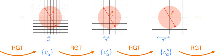
One of the most difficult challenges in lattice QCD simulations is the critical slowing down towards the continuum limit where the lattice spacing is taken to zero while keeping some physical scales fixed, cf. Fig. 1 for an illustration. The critical behaviour manifests itself in long autocorrelation times in the measurement of physical observables [1], for example gradient-flow quantities or the topological charge. The slow decorrelation in the latter quantity is usually referred to as topological freezing. While the problem is absent at sufficiently large lattice spacings, simulations at coarse resolution in general lead to large lattice artifacts and correspondingly large systematic errors due to the long extrapolation to , unless one uses highly improved lattice discretizations of the underlying theory.
One way to construct highly improved lattice actions is through renormalization group transformations (RGT). The aim of an RGT is to describe the physics of a fine lattice on a coarse lattice by means of adjusting the effective couplings of the discretized theory, cf. Fig. 1, such that the resulting effective lattice action maintains the low-energy physics exactly.
In these proceedings we describe the status of our project to construct an RG-improved lattice action which is classically perfect, i.e., which has no lattice discretization artifacts at tree level in the gauge coupling, and to employ it in Hybrid Monte Carlo (HMC) simulations. Previous reports of this ongoing project were given in [2, 3].
2 Renormalization group transformations and fixed-point actions
For gauge theories, an RGT for a lattice action from a fine to a coarse lattice can be defined through
| (1) |
where the integration on the RHS is over gauge-field configurations on the fine lattice restricted by the RG blocking kernel . In this process, the gauge coupling and the action parameterized by the couplings on the fine lattice are mapped to and , i.e., , on the coarse lattice. The RG blocking is defined as follows. First, a smeared link is constructed from the fine gauge links by adding up the original link with weight , the planar staples with weight , diagonal staples with weight , and hyper-diagonal staples with weight , as illustrated in the top row of Fig. 2. Two smeared links are then multiplied together to construct the
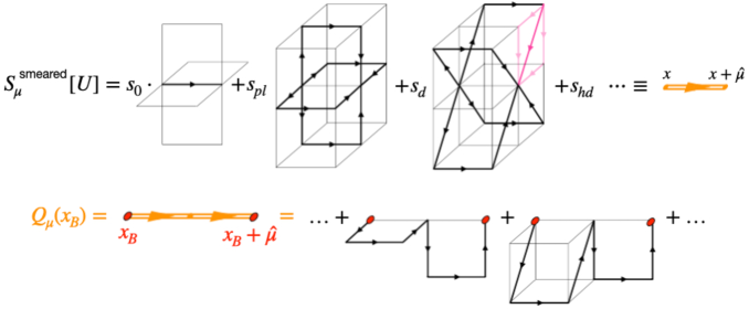
blocked link generating a combination of many gauge-link paths within 16 hypercubes of the fine lattice, cf. bottom row of Fig. 2. Finally, the gauge invariant blocking kernel is defined by
| (2) |
where the term guarantees the correct normalization of the partition function under the RGT. The parameters of the blocking kernel can be chosen to optimize the locality of
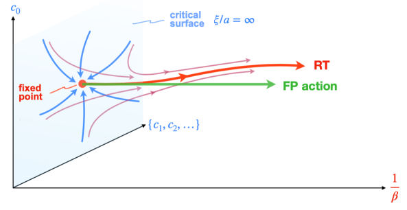
the resulting effective gauge action. For asymptotically free theories, there is one marginally relevant operator parameterized by and hence the critical surface, where , is located at . Under repeated RGT steps, any lattice action defined on the critical surface is driven to the Fixed Point (FP), cf. Fig. 3. Lattice actions slightly off the critical surface flow towards the Renormalized Trajectory (RT) which emerges from the FP along the relevant direction. Actions on the RT are effective actions with no lattice artifacts at all.
The FP at is defined by the FP equation [4]
| (3) |
and using with fixed couplings at finite defines the straight line in Fig. 3. It is expected to stay close to the RT at weak coupling and hence to have suppressed lattice artifacts. While the FP Eq. (3) implicitly provides data for each coarse configuration , finding the explicit form of the FP action, i.e., the couplings , is a difficult parameterization problem. It can be addressed efficiently using convolutional neural networks and machine-learning techniques.
3 Neural network parameterization and HMC simulation
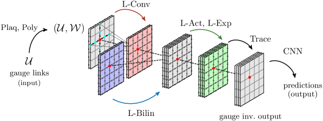
Since the FP action in general involves infinitely many gauge invariant operators with their corresponding couplings , any useful parameterization requires high flexibility while maintaining exact gauge invariance. The lattice gauge-covariant convolutional neural network (L-CNN) architecture described in Ref. [5] is well suited for this task. Taking as input a gauge field and gauge covariant objects , e.g., untraced Wilson plaquettes and Polyakov loops, the network produces arbitrarily complicated loops through convolutional layers with parallel transports, while additional bilinear layers combine products of covariant objects locally, retaining the gauge symmetry at each step. Finally, a trace layer produces gauge invariant output, cf. Fig. 4 for an illustration. We employ machine-learning techniques to train the network to reproduce the FP action values given by the RHS of Eq. (3) by parameterizing the FP action on the LHS. In addition, the derivatives of the FP action with respect to the gauge links are also determined by the FP equation, and they provide data per gauge configuration. The L-CNN generates these derivatives exactly through backpropagation, hence these large datasets are essential in training the network.
[5pt]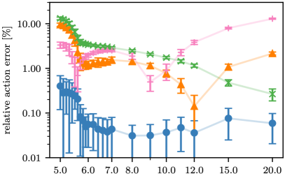 \stackunder[5pt]
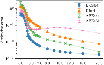
As our best parameterization, we use an L-CNN consisting of three layers with 12, 24, 24 channels and kernel sizes 2, 2, 1. In Fig. 5 we show the comparison with previous parameterizations based on traced loops up to length six and up to four powers of the traces (IIIc-4) [6], and parameterizations based on powers of traced plaquettes constructed from hypercubically APE-smeared fat links (APE444, APE431) [7]. To test the quality of different parameterizations, we take as input ensembles of coarse configurations generated with the Wilson gauge action at a range of values to cover a broad span of lattice spacings, where numerical minimization on the RHS of Eq. (3) provides the underlying true action values. The left panel shows the relative error of the parameterized FP action values on these ensembles at each indicated on the -axis, while the right panel shows the size of the parameterization errors of the derivatives. We find that the L-CNN consistently performs better than the previous parameterizations all the way from coarse to fine lattice spacing.
While an accurate parameterization is a necessary first step in the FP approach, there is no guarantee that the lattice artifacts will in fact be small when this action is used for nonperturbative calculations. This can only be tested with an actual scaling study involving MC simulations
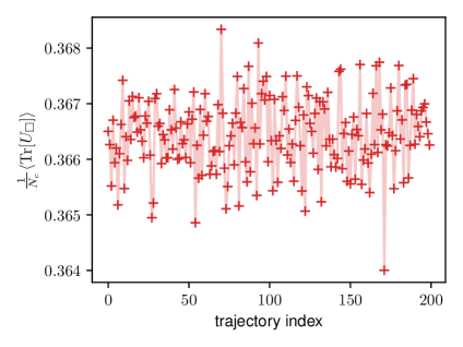
at a range of values, to make quantitative comparison with other lattice actions and the continuum limit of appropriately chosen quantities. Given that the derivatives of the FP action with respect to gauge links are automatically provided by the L-CNN through backpropagation, it is natural to choose the Hybrid Monte Carlo (HMC) algorithm [8, 9] for simulations with the FP action, adding fictitious conjugate momenta to evolve the gauge links according to the equations of motion. Standard techniques for accelerating the HMC algorithm can be used for the FP action, for example we use the 4MN4FP variant [10] of the 4th order Omelyan integrator [11] to allow for a coarser time step when solving the equations of motion. Among the tests of our implementation, we check that the Hamiltonian constraint is satisfied by ensembles generated with the HMC algorithm. We show in Fig. 6 an example of the HMC evolution of the plaquette values for a stream of 200 trajectories obtained by simulating the FP action at , which corresponds to a lattice spacing of fm.
4 Classically perfect gradient flow
A precise observable is necessary to test the quality of improvement of the FP action, without introducing additional lattice artifacts. This is naturally given by the gradient flow (GF) of the gauge fields [12, 13]. In continuum language, given the gauge action , with the field strength and gauge coupling , the non-Abelian gauge fields evolve with a fictitious time as
| (4) |
where the flow starts with the original gauge field and the flow time has dimension (length)2. The resulting action density of flowed gauge fields is renormalized, which allows a number of connections to physical quantities. For example, perturbatively the flowed action density for SU() gauge theory is
| (5) |
where is the renormalized gauge coupling in the scheme with RG scale . Hence a specific value of implicitly defines a value for the flow time in physical units, which allows the scale of lattice simulations to be determined. Another use is the gauge coupling -function defined through the GF scheme, e.g., for SU(3) gauge theory
| (6) |
where the -function can be measured directly from the GF on gauge configurations generated at chosen values of the coupling [14, 15]. In general, GF quantities can be measured with high accuracy, making them good probes of discretization effects in lattice simulations.
On the lattice, the flow is of the gauge links, with for some choice of lattice flow action. In addition, one has a separate choice of lattice action for the discretized action density observable . The gauge configurations are generated via MC simulation, where there is a third choice of discretized action . The collective discretization artifacts of these choices can be calculated perturbatively [16], with
| (7) |
where contains the tree-level lattice artifacts as deviations from 1, the action density in momentum space to quadratic order in the fields is , is the bare gauge coupling and is a gauge fixing term. One can exploit the freedom to choose different gauge actions for and to minimize the artifacts in a tree-level improved renormalized gauge coupling [16]. On the other hand, using the same lattice action for all three gives
| (8) |
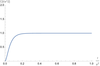
As a pedagogical guide, examples of the tree-level coefficient for two different regulators are shown in Fig. 7. One is a hard-momentum cutoff with the continuum dispersion relation, the second is the Wilson lattice gauge action for which is analytically calculable in terms of the Bessel function . For both, the coefficient approaches 1 in the limit .
For the exact FP action, the FP propagator is substituted into Eq. (8). At any finite lattice spacing, the gauge configuration can be connected back to an arbitrarily fine initial configuration through multiple RG transformations, where the propagator is also RG blocked. Although on the lattice the momenta are restricted to , the iterated RG transformations result in the FP propagator having poles at for all integers . Hence the momentum range is extended to and the exact FP propagator has the continuum dispersion relation. This results in , i.e., the exact FP action has no tree-level artifacts in the gradient flow. This new finding is in keeping with FP actions preserving classical properties exactly on the lattice, e.g., the continuum dispersion relation, exact classical (instanton) solutions and invariant topological charge under RG transformations, and chirality of FP fermions as a solution of the Ginsparg-Wilson relation [17, 18, 19].
5 Scaling of gradient-flow scales
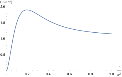
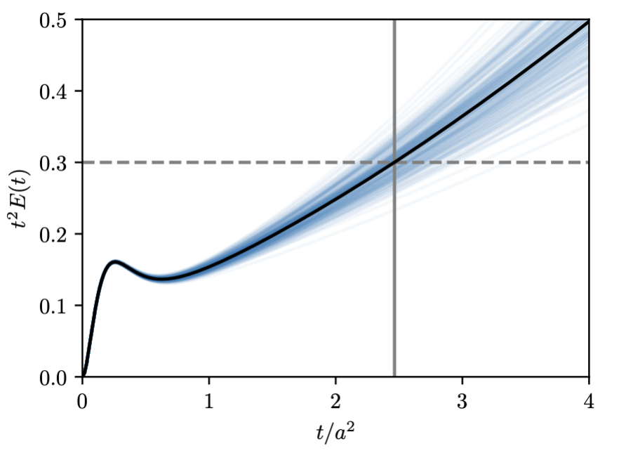
Having generated MC ensembles with the FP action, we integrate the flow equation on each configuration with the same FP action using a third-order Runge-Kutta scheme [12]. In the left plot of Fig. 8 we show the resulting flow of the action density for one FP gauge ensemble as an example. Physical reference scales are defined through the conditions [12, 20]
| (9) |
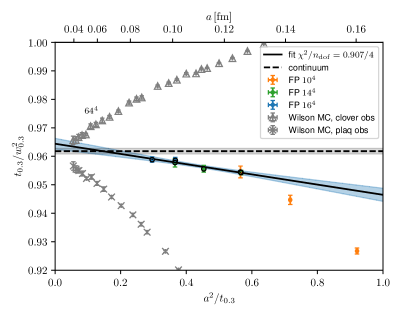
and we use the scaling of a dimensionless ratio of these scales to probe the FP action for any remaining lattice artifacts. With the classically perfect GF at hand, any such lattice artifacts are due either to an imperfect parameterization or to quantum effects. In the right plot of Fig. 8 we show the scaling of the ratio towards the continuum limit for the parameterized FP action and compare it with that of the Wilson gauge action using either the plaquette or clover discretization of the observable . We use fm [20] for a visual guide of the lattice spacing. Discretization effects in the parameterized FP action are very mild and an extrapolation of the data with fm is sufficient for a reliable continuum limit. This is in contrast to the Wilson gauge action which requires simulations at substantially smaller lattice spacings for an equally reliable extrapolation.
6 Conclusions and outlook
In this work, we have demonstrated how a fixed-point lattice gauge action can be parameterized using modern machine-learning tools, argued that the exact FP gradient flow is free of tree-level lattice artifacts, and presented preliminary results for a scaling test of the parameterized FP action through MC simulations and measurements of the gradient flow in four-dimensional SU(3) gauge theory. Lattice gauge-covariant convolutional neural networks (L-CNNs) are an essential element to achieve a superior parameterization of the FP action with exact gauge invariance. The initial results show that lattice artifacts in the parameterized FP action are much reduced, making it broadly useful for any gauge theory study, allowing continuum properties to be extracted from simulations on coarser lattices.
Acknowledgments
This work is supported in part by the Swiss National Science Foundation (SNSF) through grant No.200020208222. K.H. wishes to thank the AEC and ITP at the University of Bern for their support. A.I. and D.M. acknowledge funding from the Austrian Science Fund (FWF) projects P 32446, P 34455 and P 34764. K.H. acknowledges funding from the US National Science Foundation under grants 2014150 and 2412320. The computational results presented have been achieved in part using the Vienna Scientific Cluster (VSC) and LEONARDO at CINECA, Italy, via an AURELEO (Austrian Users at LEONARDO supercomputer) project, and UBELIX (http://www.id.unibe.ch/hpc), the HPC cluster at the University of Bern.
References
- [1] ALPHA collaboration, S. Schaefer, R. Sommer and F. Virotta, Critical slowing down and error analysis in lattice QCD simulations, Nucl. Phys. B 845 (2011) 93, [1009.5228].
- [2] K. Holland, A. Ipp, D. I. Müller and U. Wenger, Machine learning a fixed point action for SU(3) gauge theory with a gauge equivariant convolutional neural network, Phys. Rev. D 110 (2024) 074502, [2401.06481].
- [3] K. Holland, A. Ipp, D. I. Müller and U. Wenger, Fixed point actions from convolutional neural networks, PoS LATTICE2023 (2024) 038, [2311.17816].
- [4] P. Hasenfratz and F. Niedermayer, Perfect lattice action for asymptotically free theories, Nucl. Phys. B 414 (1994) 785, [hep-lat/9308004].
- [5] M. Favoni, A. Ipp, D. I. Müller and D. Schuh, Lattice Gauge Equivariant Convolutional Neural Networks, Phys. Rev. Lett. 128 (2022) 032003, [2012.12901].
- [6] M. Blatter and F. Niedermayer, New fixed point action for SU(3) lattice gauge theory, Nucl. Phys. B 482 (1996) 286, [hep-lat/9605017].
- [7] F. Niedermayer, P. Rufenacht and U. Wenger, Fixed point gauge actions with fat links: Scaling and glueballs, Nucl. Phys. B 597 (2001) 413, [hep-lat/0007007].
- [8] S. Duane, A. D. Kennedy, B. J. Pendleton and D. Roweth, Hybrid Monte Carlo, Phys. Lett. B 195 (1987) 216.
- [9] S. A. Gottlieb, W. Liu, D. Toussaint, R. L. Renken and R. L. Sugar, Hybrid Molecular Dynamics Algorithms for the Numerical Simulation of Quantum Chromodynamics, Phys. Rev. D 35 (1987) 2531.
- [10] T. Takaishi and P. de Forcrand, Testing and tuning new symplectic integrators for hybrid Monte Carlo algorithm in lattice QCD, Phys. Rev. E 73 (2006) 036706, [hep-lat/0505020].
- [11] I. P. Omelyan, I. M. Mryglod and R. Folk, Symplectic analytically integrable decomposition algorithms: classification, derivation, and application to molecular dynamics, quantum and celestial mechanics simulations, Comput. Phys. Commun. 151 (2003) 272.
- [12] M. Lüscher, Properties and uses of the Wilson flow in lattice QCD, JHEP 08 (2010) 071, [1006.4518].
- [13] M. Luscher and P. Weisz, Perturbative analysis of the gradient flow in non-abelian gauge theories, JHEP 02 (2011) 051, [1101.0963].
- [14] Z. Fodor, K. Holland, J. Kuti, D. Nogradi and C. H. Wong, A new method for the beta function in the chiral symmetry broken phase, EPJ Web Conf. 175 (2018) 08027, [1711.04833].
- [15] A. Hasenfratz and O. Witzel, Continuous renormalization group function from lattice simulations, Phys. Rev. D 101 (2020) 034514, [1910.06408].
- [16] Z. Fodor, K. Holland, J. Kuti, S. Mondal, D. Nogradi and C. H. Wong, The lattice gradient flow at tree-level and its improvement, JHEP 09 (2014) 018, [1406.0827].
- [17] T. A. DeGrand, A. Hasenfratz, P. Hasenfratz and F. Niedermayer, The Classically perfect fixed point action for SU(3) gauge theory, Nucl. Phys. B 454 (1995) 587, [hep-lat/9506030].
- [18] P. Hasenfratz, Lattice QCD without tuning, mixing and current renormalization, Nucl. Phys. B 525 (1998) 401, [hep-lat/9802007].
- [19] P. Hasenfratz, V. Laliena and F. Niedermayer, The Index theorem in QCD with a finite cutoff, Phys. Lett. B 427 (1998) 125, [hep-lat/9801021].
- [20] BMW collaboration, S. Borsányi, S. Dürr, Z. Fodor, C. Hoelbling, S. D. Katz, S. Krieg et al., High-precision scale setting in lattice QCD, JHEP 09 (2012) 010, [1203.4469].