Hypercyclicity of Toeplitz operators with smooth symbols
Abstract.
This paper is devoted to the study of the dynamics of Toeplitz operators with smooth symbols on the Hardy spaces of the unit disk , . Building on a model theory for Toeplitz operators on developed by Yakubovich in the 90’s, we carry out an in-depth study of hypercyclicity properties of such operators. Under some rather general smoothness assumptions on the symbol, we provide some necessary/sufficient/necessary and sufficient conditions for to be hypercyclic on . In particular, we extend previous results on the subject by Baranov-Lishanskii and Abakumov-Baranov-Charpentier-Lishanskii. We also study some other dynamical properties for this class of operators.
Key words and phrases:
Toeplitz operators, hypercyclicity, linear dynamics, eigenvectors of Toeplitz operators, model theory for Toeplitz operators, Smirnov spaces2010 Mathematics Subject Classification:
47B35, 47A16, 30H10, 30H151. Introduction and main results
Our aim in this paper is to investigate Toeplitz operators on the Hardy space of the open unit disk , where , from the point of view of linear dynamics.
Given a function , where denotes the unit circle in , the Toeplitz operator on is defined by
Here denotes the canonical (Riesz) projection from onto , and it is well-known that it is bounded when . Then the Toeplitz operator is bounded on , which we denote by . The class of Toeplitz operators plays a prominent role in operator theory, partly because of their numerous applications to various other domains such as complex analysis, theory of orthogonal polynomials, probability theory, information and control theory, mathematical physics, etc. We refer the reader to one of the references [BottcherSilbermann1990, Nikolski-2020, Hartmann-2016, Basor-Gohberg-1994, Brown-Halmos, Nikolski-2002-1, Nikolski-2002-2, Douglas-1972] for an in depth study of Toeplitz operators from various points of view. See also Appendix A for some useful reminders on Toeplitz operators and the Riesz projection .
Our focus here will be on the study of the hypercyclicity of Toeplitz operators on spaces, as well as of related properties such as chaos, frequent hypercyclicity, ergodicity… Definitions as well as related concepts will be presented in the forthcoming sections and in Appendix A. Any unexplained terminology pertaining to linear dynamics can be found in one the books [BayartMatheron2009] or [GrosseErdmannPeris2011], together with a thorough presentation of linear dynamical systems, both from the topological and from the measurable point of view. It may be useful to mention that the main difficulty when studying the dynamics of Toeplitz operators is that, in general, explicit formulas for the powers of the Toeplitz operator are not available, except when the symbol is analytic or anti-analytic.
Given a bounded operator acting on a (real or complex) separable Banach space , is said to be hypercyclic on if it admits a vector with a dense orbit . Such a vector is called a hypercyclic vector for . Hypercyclicity is clearly a reinforcement of the classical notion of cyclicity, where one requires the existence of a vector such that the linear space of its orbit is dense in . A hypercyclic operator satisfies the following spectral properties: every connected component of its spectrum intersects the unit circle, and the point spectrum of its adjoint is empty. In particular, it easily follows that a Toeplitz operator with an analytic symbol is never hypercyclic. On the other hand, many operators can be shown to be hypercyclic, based on the study of their eigenvectors. Indeed, a well-known criterion due to Godefroy and Shapiro [GodefroyShapiro1991] states the following:
Suppose that the two spaces
| (1.1) |
are equal to . Then is hypercyclic on .
This criterion will be used repeatedly in the paper to show that for large classes of symbols , the associated Toeplitz operator on is hypercyclic.
The study of Toeplitz operators from the point of view of linear dynamics began in the seminal work of Godefroy and Shapiro [GodefroyShapiro1991], where they gave a necessary and sufficient condition for the adjoint of a multiplication operator on to be hypercyclic, thus characterizing hypercyclic Toeplitz operators with anti-analytic symbols: if and is not constant, then is hypercyclic if and only if . The next step was done by Shkarin, who considered in [Shkarin2012] the case where
and proved that is hypercyclic on if and only if and the bounded component of intersects both and . Baranov and Lishanskii investigated next in [BaranovLishanskii2016] the more general case where has the form
where is an analytic polynomial and belongs to . They provided some necessary conditions (of a spectral kind) for to be hypercyclic on , as well as some sufficient conditions, based on the study of the eigenvectors of and on the Godefroy-Shapiro Criterion. The same line of approach was taken in the subsequent work [AbakumovBaranovCharpentierLishanskii2021] of Abakumov, Baranov, Charpentier and Lishanskii, where the authors extended results of [BaranovLishanskii2016] to the case of more general symbols of the form
where is a rational function without poles in and belongs to . The novel feature of the approach taken in [AbakumovBaranovCharpentierLishanskii2021] is the use of deep results of Solomyak [Solomyak1987] providing necessary and sufficient conditions for finite sets of functions in to be cyclic for some analytic Toeplitz operators on . Taken in combination with the description of some eigenvectors of , this yields substantial extensions of certain results from [BaranovLishanskii2016].
Our work is a further contribution to the study of hypercyclicity of Toeplitz operators. Our approach here is somewhat different from the ones taken in the previous works mentioned above, although we will use too properties of eigenvectors and the Godefroy-Shapiro Criterion in order to obtain sufficient conditions for to be hypercyclic. So as to exhibit suitable families of spanning eigenvectors for , we rely on deep constructions by Yakubovich of model operators for Toeplitz operators on with smooth symbol. It should be mentioned that the model theory for Toeplitz operators with smooth symbols has a rich history. See for instance [Clark-1980-1, Clark-1980-2, Clark-1981, Clark-1987, Clark-1990, Clark-Morrel-1978, Duren-1961, Peller-1986, Wang-1984]. In a series of papers culminating in the works [Yakubovich1991] and [Yakubovich1996] (see also [Yakubovich1989, Yakubovich1993]), Yakubovich showed that for a very large class of positively wound smooth symbols on , the operator is similar to a direct sum of multiplication operators by the independent variable on certain closed subspaces of Smirnov spaces , where the sets are suitable unions of connected components of . In the case where the symbol is negatively wound, in an analogous way is similar to the direct sum of the adjoints of these multiplication operators on these subspaces of the ’s. In particular, under these conditions, admits an functional calculus on the interior of the spectrum of . Moreover, using this model, Yakubovich proved in [Yakubovich1991] and [Yakubovich1996] that whenever is sufficiently smooth and negatively wound, is cyclic on . The proof of this last property relies on the fact that the eigenvectors of associated to eigenvalues span a dense subspace of .
It is not difficult to see (see Proposition 3.1 below) that, for smooth symbols at least, a necessary condition for the hypercyclicity of is that be negatively wound. We will suppose that it is the case in the rest of this introduction.
Thus, in order to decide whether the Godefroy-Shapiro Criterion can be applied to (proving then hypercyclicity), we need to find conditions on a subset of implying that the vector space
is dense in . In other words, given any (where is the conjugate exponent of ), we need to be able to decide wether as soon as is vanishes on the eigenspaces for all . An easy observation, based on the analyticity of the eigenvector fields and the Uniqueness Principle for analytic functions (see Proposition 2.5 for details), shows that if vanishes on for all , then vanishes on for all , where is any connected component of such that has an accumulation point in . Recall that we do know (as mentioned above, it is a consequence of results from [Yakubovich1991] and [Yakubovich1996]) that if for every connected component of and for every , vanishes on , then . So things boil down to the following kind of question, which we state here informally:
Question 1.1.
Let be a connected component of and let be such that
Let be another connected component of . Under which conditions on and is it true that
We will investigate this question in some depth, finding rather general conditions on pairs of connected components of implying an affirmative answer to 1.1. This will allow us to derive necessary and sufficient geometrical conditions implying the hypercyclicity of under fairly general conditions on the (negatively wound) symbol . Moreover, this approach allows us to treat the case where acts on rather than the Hilbertian case only.
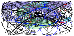
Our conditions are stated essentially in terms of smoothness of the symbol , which is at least required to belong to a class , for some suitable (see Section A.2 for the definition of ) and of geometrical properties of the set of connected components of . Rather than state here formally some of our results, which would require some preparation and notation, we prefer to present in an informal way some cases where we are able to characterize hypercyclicity of , along with a picture of a situation where we are in the case considered and is hypercyclic.
Let and its conjugate exponent, i.e. . Consider the following conditions on the symbol :
-
(H1)
belongs to the class for some , and its derivative does not vanish on ;
-
(H2)
the curve self-intersects a finite number of times, i.e. the unit circle can be partitioned into a finite number of closed arcs such that
-
(a)
is injective on the interior of each arc ;
-
(b)
for every , the sets and have disjoint interiors;
-
(a)
-
(H3)
for every , , where denotes the winding number of the curve around .
-
(H4)
for every , admits an analytic extension on a neighborhood of the closed subarc , where the arcs are given by 2.
When condition 2 is satisfied, denote by the set of all the images by of the extremities of the arcs . The set of self-intersection points of the curve is contained in , hence finite. By choosing the arcs in a suitable manner, it is possible to ensure that is exactly the set of self-intersection points of ; this is what we will assume in the forthcoming sections. Under assumption 2, the function admits an inverse defined on . Let us note that the results that we will obtain will depend only on the a.e. behaviour of the function on ; in particular, they do not depend on the specific form of the set induced by the choice of the arcs in assumption 2.
The smoothness and injectivity conditions 1 and 2 are those from [Yakubovich1991] in the case . A more general condition than 2, allowing the sets and to coincide for some indices , is provided in [Yakubovich1996]. Some of our results also hold under this weaker assumption, but for simplicity’s sake, we begin by restrict ourselves here to the case where 2 holds, i.e. to the case where the curve has only a finite number of auto-intersection points. The weaker assumptions of [Yakubovich1996] will be considered in Section 6. Let satisfies the first three assumptions 1, 2 and 3. Recall (see Lemma A.11) that in this case
We denote by the set of all connected components of . For every , let be the common value of We will prove (see Theorem 3.2) that a necessary condition for , acting on , to be hypercyclic, is that intersects every connected component of the interior of . Here are now some examples of necessary/sufficient/necessary and sufficient conditions that we obtain for the hypercyclicity of on :
-
Case 1:
If for every , then is hypercyclic on (Theorem 4.1). See Figure 1.
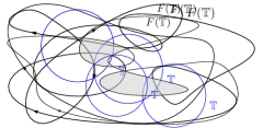
Figure 1. -
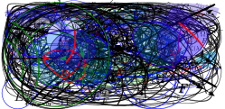
Case 2:
If has only one element, i.e. is connected, then is hypercyclic on if and only if (Theorem 5.1). See Figure 2.

Figure 2. -
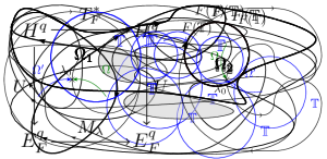
Case 3:
If is finite for all distinct elements of , then is hypercyclic on if and only if for every (Theorem 5.5). See Figure 3.
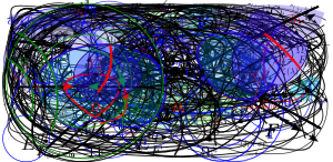
Figure 3. -
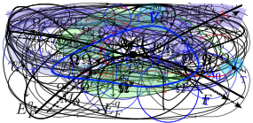
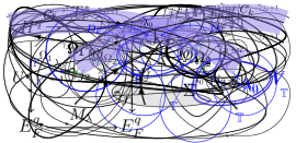
Case 4:
Say that is a maximal component of if the following holds: for every which is adjacent to , .
If intersects all the maximal components of , then is hypercyclic on (Theorem 5.6). See Figure 4.
Figure 4. -
Case 5:
Suppose that satisfies the additional assumption 4 and that the following holds: for every pair of adjacent connected components of with , one of the following properties holds:
-
(a)
there exists a self intersection point of the curve and an open neighborhood of such that: , belongs to , and the restriction of the function to cannot be extended continuously at the point ;
-
(b)
is a Jordan curve and there exists a closed arc of such that and has an analytic extension on a neighborhood of .
Then is hypercyclic on if and only if intersects every component of (Theorem 5.14). See Figure 5.

Figure 5. -
(a)
Our results allow us to retrieve and generalize previous results from [Shkarin2012], [BaranovLishanskii2016] and [AbakumovBaranovCharpentierLishanskii2021] on hypercyclicity of Toeplitz operators on , up to one important point: while our results apply to general smooth functions on , those of [AbakumovBaranovCharpentierLishanskii2021] apply to symbols of the form where is a rational function without poles in and belongs to the disk algebra , the space of functions which are analytic on and admit a continuous extension to . While the restriction of to is as smooth as we wish, that of is only continuous, so that the restriction of to may be only continuous. See Section 7 for details.
The paper is organized as follows: in Section 2, we first present Yakubovich’s results on models for Toeplitz operators with negatively wound symbols on , and state their extension to the setting that will be required in the sequel of the paper. In Section 3, we present some necessary conditions for the hypercyclicity of Toeplitz operators on . Sections 4 and 5 are devoted to the proofs of our main results, providing sufficient as well as necessary and sufficient conditions for the hypercyclicity of these operators. The more general case where the symbol is not necessarily required to be injective on the circle minus a finite number of points (i.e. the setting of [Yakubovich1996]) is discussed then in Section 6. In Section 7, we compare our results and approach to those taken by Abakumov, Baranov, Charpentier and Lishanskii in [AbakumovBaranovCharpentierLishanskii2021]. Section 8 contains some generalizations and further results, as well as some open questions arising from our study. In particular, we investigate in Section 8 other notions in linear dynamics such as supercyclicity, chaos, frequent hypercyclicity and ergodicity with respect to an invariant ergodic measure in the setting of Toeplitz operators.
The paper also contains two appendices: the first one, Appendix A, presents some reminders on topics and tools which are repeatedly used in the paper: basics on the Fredholm theory of Toeplitz operators, Carleson measure, Smirnov spaces, quasiconformal maps, Privalov’s type theorems, and, lastly, linear dynamics. The second one, Appendix B, contains a full proof of the extension to the case of the main results from [Yakubovich1991] on Toeplitz operators. Our approach follows closely that of [Yakubovich1991], and we do not make any claim for originality here. However, since these results are extremely beautiful, but not so easy to read in their original presentation, we thought it worthwhile to provide a detailed account of them, and of their extension to the setting.
Acknowledgments. We aall re grateful to Dmitry Yakubovich for stimulating discussions on the topic of this paper, and in particular for pointing out us the simplification in the proof of Proposition 4.8 given in Remark 4.10. We also thank Dmitry Khavinson for providing us with useful references on Smirnov spaces.
2. Model theory for Toeplitz operators on spaces with smooth symbols
In this section we present the notation, setting and main results from [Yakubovich1991] and [Yakubovich1996] (in the -case) which are crucial to our approach to hypercyclicity properties of Toeplitz operators on . We’ll restrict ourselves here to the bare essentials, see Appendix B for further details, explanations and proofs.
For , let denote the Hardy space of all analytic functions on the open unit disk such that
A function has non tangential boundary values almost everywhere on . We will often still denote this boundary value as . It is well-known that . The dual of is canonically identified to , where is the conjugate exponent of and the duality is given by the following formula:
| (2.1) |
where and . This duality bracket is linear on both sides; we keep this convention even when , so that in particular adjoints of operators on must be understood as Banach space adjoints, and not Hilbert space adjoints.
We denote by the Riesz projection from into defined by
2.1. Some spectral theory
Given , the Toeplitz operator on defined by , is bounded on . Suppose that is continuous on . Then is a Fredholm operator on if and only if ; in this case, its Fredholm index is equal to and we can describe the spectrum of as
where is the winding number of the curve with respect to the point . See Lemma A.11. Note that if is at least on (which is the case in the whole of this paper), the winding number is given by
By continuity of the winding number, the function is constant on each connected component of . We denote this common value by .
2.2. Eigenvectors
Suppose now that takes only non positive values on , i.e. that assumption 3 from the introduction is satisfied. It then follows from the version of the Coburn Theorem (Theorem A.12) and Lemma A.11 that, for every ,
Henceforward, we assume that satisfies assumptions 1, 2 and 3. In order to represent as the adjoint of a multiplication operator by on a certain space of analytic functions, Yakubovich provided in [Yakubovich1991] an explicit expression of a spanning family of elements of . Let , and consider the function defined on by
Since is and does not vanish on , and since , one can define a logarithm of on that is on , and set
| (2.2) |
More details on the construction on are contained in Appendix B. The functions and both belong to and for every connected component of and every , the map is analytic on and continuous on (see Lemma B.1 and Lemma B.9 for details).
Let and for each , let
| (2.3) |
be the set of points in where the (negative) winding number of is strictly less than . We have
and (which is the set of all ’s in such that is Fredholm) coincides with . Note also that
For every and every , set
| (2.4) |
These functions belong to , hence to , and it can be checked that for every . So, we have
for every (see Lemma B.4). Moreover, the map is analytic from into and, for a fixed , the function belongs to the Smirnov space , where is the conjugate exponent of (see Theorem B.15).
The reader may wonder why we normalize the eigenvectors in Equation 2.4 by the constant . In fact, in the construction of the model, we would like that the isomorphism which implements the model satisfies that (see Equation 2.7) and, since , this imposes this constant. With this property for , it turns out that one can obtain an explicit formulae for the inverse of . See [Yakubovich1991] for more explanations on this point.
2.3. Interior and exterior boundary values
Assumption 2 implies that the curve has only a finite number of points of self-intersection which is the set . Whenever is a subarc of containing no point of , is included in the boundary of exactly two connected components and of , and we have
If , we say that is the interior component and is the exterior component (with respect to ). Now, let be continuous on . For , let be a small subarc of containing . We define (when they exist) the following non-tangential limits, called respectively the interior and exterior boundary values of at :
where and are respectively the interior and exterior connected components with respect to . Functions in a Smirnov space of a domain of (with a rectifiable boundary ) admit non-tangential limits almost everywhere on (see Section A.5). If and are two adjacent domains along an arc , and if belongs to some Smirnov space , then the interior and exterior boundary values and exist almost everywhere on (see Figure 6).

With these notations, suppose that satisfies 1, 2 and 3. Since is invertible from onto , one can define the map on . In particular, is defined almost everywhere on . Then (see Corollary B.12) the eigenvectors of given by (2.4) satisfy the following relation: for every , we have
| (2.5) |
2.4. Boundary conditions in some Smirnov spaces
Let . On the direct sum , we consider the following norm:
Note that for each connected component of , the non-tangential limit of the function exists almost everywhere on the boundary of and that for every , the non tangential limits and exist almost everywhere on .
Let be the closed subspace of formed by the -tuples in satisfying, for all ,
| (2.6) |
Note that Equation 2.5 implies that for all , the -tuple belongs to . Note also that this subspace is an invariant subspace for the multiplication operator defined by
More generally let be a bounded analytic function on the interior of the spectrum of . Then the space is invariant by the multiplication operator on defined by , where for every . This means that is contained in the multiplier algebra of .
2.5. The main result of Yakubovich
After all this preparation, we are now ready to define the operator that gives as a model operator for .
Let , and let be the conjugate exponent of (i.e. ). Suppose that the symbol of the Toeplitz operator satisfies 1, 2 and 3. Let , , be given by (2.4). For every function , define by setting
| (2.7) |
Note that, since is an eigenvector of associated to the eigenvalue , we have for every and every that
In other words,
Since the functions , , form a basis of the eigenspace , it follows that
Fact 2.1.
For any , vanishes on if and only if for every .
We are now ready to give the version of the main result of Yakubovich in [Yakubovich1991].
Theorem 2.2.
The operator defined above is a linear isomorphism from onto . Moreover, we have
In other words, the following diagram commutes:
![[Uncaptioned image]](/html/2502.03303/assets/x7.png)
This model is built from eigenvectors of , and the relation means nothing else than this. See the introductions of the papers [Yakubovich1991, Yakubovich1993] for insightful comments on this construction. A detailed proof of Theorem 2.2 will be given in Appendix B.
We conclude this section with some important consequences of Theorem 2.2.
2.6. The functional calculus
Since is contained in the multiplier algebra of , a first important consequence of Theorem 2.2 is the existence of an functional calculus for on the interior of the spectrum of .
Corollary 2.3 (Yakubovich [Yakubovich1991]).
Indeed, let . By Theorem 2.2, we can set . This defines a functional calculus for on , and
See Theorem B.25. Set now for every ; this defines an functional calculus for on the interior of , and Corollary 2.3 follows.
2.7. Spanning eigenvectors
The second important consequence of Theorem 2.2 is that eigenvectors of span a dense subset of . Before we justify this statement, we set a notation which will be used repeatedly throughout this work.
Definition 2.4.
Let denote the set of all connected components of . For every , set
| (2.8) |
Here is now a result which will be crucial in the sequel.
Proposition 2.5.
Proof.
Given , observe that the functions , , are analytic on (they belong to ) and span a dense subspace of . Then the uniqueness principle for analytic functions yields (1). In order to prove (2), suppose that vanishes on all eigenspaces . Then we have, for every ,
This means exactly that , and since is injective by Theorem 2.2, . ∎
This consequence of Theorem 2.2 is used in [Yakubovich1991] to derive the cyclicity of under the assumptions 1, 2 and 3. Indeed, since for every , it follows from Proposition 2.5 and Lemma A.21 that is cyclic. In order to investigate the hypercyclicity of , an important part of our work will be to refine Proposition 2.5, to as to be able to conclude (under suitable conditions on the symbol ), that
These two properties will allow us to apply the Godefroy-Shapiro Criterion, and thus to deduce that is hypercyclic on . This will be the main goal of our Section 4. Applications will be presented in Section 5. Meanwhile, we present some necessary conditions (of a spectral nature) for the hypercyclicity of .
3. Necessary conditions for hypercyclicity of Toeplitz operators
3.1. A condition on the winding number
A first observation is that for a sufficiently smooth symbol , has to be negatively wound for to have a chance of being hypercyclic.
Proposition 3.1.
Let be continuous on and let . If there exists a point with , then is not hypercyclic on .
Proof.
Recall (see Lemma A.11) that, since , is a Fredholm operator, and its Fredholm index satisfies
Thus
Then is an eigenvalue for . But the adjoint of an hypercyclic operator must have empty point spectrum, and hence cannot be hypercyclic. ∎
Assumption 3 is thus natural in our context.
3.2. Intersection with connected components of the interior of the spectrum
It is also well-known (see Section A.6) that whenever is a hypercyclic operator on a complex separable Banach space , every connected component of the spectrum of must intersect the unit circle . It turns out that, in our current setting, a stronger property must hold.
Theorem 3.2.
For instance, in the situation represented in Figure 7, Theorem 3.2 states that for to be hypercyclic, the unit circle must intersect all the “petals” of the flower-like domain - which is much stronger that requiring that , which is connected here, intersects .

Theorem 3.2 follows immediately from Proposition 3.3 below, which has some independent interest, and the fact that under assumptions 1, 2 and 3, has an -functional calculus (Corollary 2.3).
Proposition 3.3.
Let be a complex separable Banach space, and let be hypercyclic. Suppose that admits an -functional calculus on a certain open subset of , and that all connected components of intersect . Then every connected component of intersects .
Proof.
Let be a connected component of , and let . Define a function on by setting if and if . Set . Then and are elements of . Set . The ’s are well-defined bounded projections on , with and . Denote by the range of . Then is a closed -invariant subspace of and . If has at least two connected component, intersects both and , , and then is a non-trivial projection. So and . If is connected, then and . Denote by the operator induced by on , . Then
Fact 3.4.
We have .
Proof of 3.4.
Since , we clearly have . If , define a function by setting , . Then , and the operator leaves invariant and satisfies for every . So is invertible on , and . Thus . Suppose now that . Then (because is open and ), and by the argument above . Since , necessarily , so that . Hence and this shows that . ∎
Moreover, since the operator admits an -functional calculus, admits an -functional calculus. Let . Then can be extended into a function by setting for . For , define
| (3.1) |
Then is a bounded operator on and we have
for a positive constant independent of . Then we easily see that Equation 3.1 defines an -functional calculus for . Since is a hypercyclic operator on , the operator is also hypercyclic on (see Lemma A.13).
Let us finally show that it is impossible to have nor . If , then
so that is a power-bounded operator on . This stands in contradiction with the hypercyclicity of . If now , then since , is invertible, and so is also hypercyclic (see Section A.6). Since , by the functional calculus again, we have that
contradicting the hypercyclicity of . So and , i.e. . ∎
4. Proving the hypercyclicity of : from a connected component to another
We remind the reader that denotes the set of all connected components of ; we also recall that the spaces and are defined in Equation 1.1, and the spaces for in Equation 2.8. Let us begin with the easiest case where can be shown to be hypercyclic.
Figure 8 illustrates an example of a situation where has two connected components and Theorem 4.1 applies:

Proof.
Theorem 4.1 is an immediate consequence of Proposition 2.5. Indeed, since for every , and both have accumulation points in for every and then, for every ,
Hence and for every . So by Proposition 2.5, we deduce that , and the conclusion follows from the Godefroy-Shapiro Criterion. ∎
What happens now if, in Figure 8, intersects only one of these two connected components and ? There are at least two kinds of situations which have to be considered.
-
Case a:
the case where intersects the component , but not the component as is Figure 9.
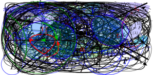
Figure 9. -
Case b:
the case where intersects but not as in Figure 10.

Figure 10.
In the first case, since has accumulation points in both and , according to Proposition 2.5, we have . However, we only know a priori, by Proposition 2.5 again, that contains the subspace , and in order to be able to conclude that , we would need to have also that
This would obviously be true provided that
and then Proposition 2.5 would imply that .
In the second case, the easy fact is that and it is true that . So what we would need in order to obtain that is that
Observe that one can also have a mix of these two situations, where the unit circle is contained in the boundary of both and as in Figure 11.

Going back to our general situation, let us say that two connected components are adjacent is there exists an arc with non-empty interior contained in . In this case, the winding numbers and differ by exactly. The main problem we are facing is the following:
Question 4.2.
Let and be two adjacent components of . When is it true that
As illustrated by the example in the next subsection, the difficulty of this question varies, depending on whether (meaning that is the interior component and is the exterior component with respect to ) or (meaning that is the interior component and is the exterior component).
In our study of 4.2, the boundary conditions in Equation 2.6 defining the subspace of (where is the operator defined in Section 2) will play a crucial role. As a consequence, we will often use the following uniqueness property of functions belonging to Smirnov spaces (which is also recalled in Section A.5):
Fact 4.3.
Let be a bounded simply connected domain and let . Let . Then admits a non-tangential limit almost everywhere on If on a subset of of positive measure, then on .
4.1. Example of two circles

Our aim here is to show, using the explicit expression of the function on which is available in this case, that is hypercyclic on .
Observe that
which is equivalent to say that
Observe now that . Hence, for , let be such that . We have , and since , we get that . So we deduce that
Let and write as , where and . Then and satisfy almost everywhere on (see Equation 2.6). Note that, with respect to , is the exterior component and is the interior component.
Suppose that vanishes on . Since , we have
So almost everywhere on , and thus the boundary relation becomes
Since and its non-tangential limit is zero on a subset of with positive measure, we deduce that on . This means that vanishes on . So vanishes on and , and by Proposition 2.5, we deduce that and that .
Suppose now that vanishes on . Since , vanishes on , i.e.
Then almost everywhere on and the boundary relation becomes
The function admits an analytic extension to , given by
| (4.2) |
where is an analytic branch of the logarithm with imaginary part in . Note that this extension is such that
| (4.3) |
Since is analytic and bounded on , the function belongs to , and since we have almost everywhere on , which is a subset of of positive measure, we deduce that on .
If we suppose now that is not identically zero on , there exists a point such that does not vanish on a neighborhood of . Thus
and this contradicts Equation 4.3. So on and thus on as well. This means that vanishes on , so and thus .
Hence we have shown that and, by the Godefroy-Shapiro Criterion, the operator is hypercyclic on .
This example highlights the fact that when we need to go from a connected component to an adjacent one with a lower winding number, the situation is quite simple, whereas going to an adjacent component with a higher winding number becomes substantially more difficult.
4.2. From the interior to the exterior
The easiest case is the first one, when is the exterior component of and is the interior one. In this case, 4.2 always admits an affirmative answer.
Theorem 4.4.
Proof.
Suppose that vanishes on , i.e. that for every and every . Set , so that . Denoting by the operator from Theorem 2.2 and setting with for , our assumption on can be rewritten as on for every .
The assumption means that is the interior component of and is the exterior one. It follows that
so that, for every , and almost everywhere on .
The functions satisfy the boundary relations
Since for every , it follows that and
so that almost everywhere on . Now is a subset of positive measure of and for every , so on for every . Since ,
i.e. vanishes on all the eigenspaces with . So vanishes on , and Theorem 4.4 is proved. ∎
4.3. From the exterior to the interior
Thus one can always “go up” from one component of to an adjacent one. We now need to “go down”, i.e. to deal with the case where . Here the situation is more intricate, and we are able to show that only under stronger assumptions, concerning both the smoothness of the function and a certain geometric property 1 of the boundaries of the domains and .
Let be two adjacent components of along an arc such that . We say that the pair satisfies the property 1 if the following holds:
-
(P)
there exists a self-intersection point of the curve and an open neighborhood of such that:
-
(i)
is the only adjacent component of in a neighborhood of the point , i.e. ;
-
(ii)
belongs to , and the restriction of the function to cannot be extended continuously at the point ;
-
(iii)
there exists a simple closed curve with such that separates into two connected components and admits a bounded analytic extension on .
-
(i)
The meaning of the geometric assumption 1 may be somewhat difficult to grasp. Let us first explain how one can see whether an intersection point on satisfies or not properties (i) and (ii) of 1. These two properties involve the behavior of in a neighborhood of . Recall that is constructed from (we have indeed on ), so in each direction of the curve near , admits a limit. For example, in Figure 13, in two different directions, the limits are , and in the other two directions, the limits are .
For to satisfy properties (i) and (ii) of 1, we require that on , it is possible to approach from two different directions, and that the limits in these two directions are not the same. As a result, it will not be possible to extend to in such a way that it is continuous at . This means that we are not in the situation of Figure 14(a). We also require that there is a neighborhood of such that , i.e. is the only adjacent component of in a neighborhood of . So, if for example the intersection at the point is simple, then we cannot be in the situation described in Figure 14(b). If the intersection at the point is not simple, then there is no component inside which would also have as a boundary point, i.e. we are not in the situation in Figure 14(c).

An intersection point on which satisfies the assumptions (i) and (ii) in 1 is a point where we have the type of situation represented in Figure 15.
Observe that when satisfies assumptions 1, 2 and 4, the property (iii) in 1 is automatically satisfied. Indeed, we have:
Fact 4.5.
Note that examples such as the ones considered in Section 4.1 satisfy the hypothesis 1, 2 and 4 and thus also (iii) of property 1.
Proof.
Let be closed arcs of , with disjoint interiors, covering the circle and which are given by assumption 2. Without loss of generality, each arc can be written as
where and . Since satisfies 4, there exists for every a neighborhood of the closed arc such that admits an analytic extension on . Since for every , for every point , and hence is a local biholomorphism at every point , including the extremities and of .
Let now , and let
For each , is an extremity of the two arcs and , with . Let and be open neighborhoods of and respectively such that and are biholomorphisms, with . We denote by and their respective inverses. We have for every and for every . Suppose now that , i.e. that for some . Since the restriction of to coincides with , we have . But , is injective on , and and both belong to , and thus . If follows that and coincide on . In the same way, and coincide on (see Figure 16).

Let now , which is an open neighborhood of . Let be a connected component of . Making smaller if necessary, we can assume that and that consists of two arcs intersecting at the point , as in Figure 16 above. Let be any simple closed curve (for instance a segment) with which separates in two components and intersects at the point only. Let now and with and be such that and . Then and coincide on , while and coincide on . It follows that the function defined on by setting
is a bounded analytic extension to of the restriction of to . ∎
In some circumstances, we are able to handle situations where 1 does not hold. We will get back to this at the end of this section, and also provide some examples in Section 5.
Theorem 4.6.
As a direct consequence of Theorems 4.6 and 4.4, we have the following result.
Corollary 4.7.
Proof of Theorem 4.6.
The beginning of the proof of Theorem 4.6 is the same as that of Theorem 4.4. Let which vanishes on Set and define with , . We know that Now the assumption means that is the interior component of and is the exterior component of . Let . Since , , and we have for every . So, according to Equation 2.6, we have
Now almost everywhere on for every , and hence
We would like to be able to deduce from this relation that on for every with . It is here that the assumptions 1 come into play. We state separately as Proposition 4.8 the result we will need in order to conclude the proof.
Proposition 4.8.
Let . Suppose that satisfies 1, 2 and 3, and let on . Fix . Suppose that there exists which is a point of self-intersection of the curve such that for every sufficiently small open neighborhood of , there exists a connected component of such that
-
(a)
the restriction of to cannot be extended continuously at the point ;
-
(b)
there exists a simple closed curve with such that separates into two connected components and admits a bounded analytic extension on .
Let , and let . If almost everywhere on , then
Note that the condition on in Proposition 4.8 implies that for every neighborhood of , we can find a connected component of such that cannot be written as the image by of exactly one arc in . Also note the following: if the assumptions of Theorem 4.6 are satisfied, if we set and if is any sufficiently small neighborhood of the point , then is always a connected set, so that the assumptions of Proposition 4.8 are satisfied with .
Taking Proposition 4.8 for granted, let us explain how we conclude the proof of Theorem 4.6. For every , the functions and belong to and respectively. Since for every , we have , and thus and both belong to . We apply Proposition 4.8 to , and given by the assumption 1, , and . We have almost everywhere on , hence almost everywhere on . Now by assumption 1, . So almost everywhere on . Proposition 4.8 applies, and yields that on .
We have proved that and vanish on for every , which is the conclusion we were looking for: vanishes on for every , and so . ∎
It remains to prove Proposition 4.8.
Proof of Proposition 4.8.
In agreement with assumption 2, let be closed arcs of with disjoint interiors which cover the circle. Without loss of generality, we can write each arc as
where and . We set , so that
The self-intersection points of the curve are to be found among the points . Whenever is a self intersection point of the curve, we set
Then contains at least two elements. If we enumerate as for some , where , then for each , belongs to the arcs and , where . See Figure 17.

Let and be given satisfying the assumptions of Proposition 4.8. We know that the restriction of the function to cannot be extended continuously at the point . Reducing if necessary, it follows that there exist two integers and such that
| (4.4) |
and What it means is best seen on a picture as in Figure 18 with for example and :

Since almost everywhere on , almost everywhere on . Let be a curve given by the hypothesis of Proposition 4.8 and containing the point , and let . Reducing again if necessary, we can assume that consists of two arcs intersecting at the point , that has exactly two components and that has a bounded analytic extension on . We denote by the component containing the set , and by the component containing the set . See Figure 19.

Since and is bounded on , . Our assumption that almost everywhere on implies that almost everywhere on , which is a subset of with positive measure. Hence on by the uniqueness property of Smirnov functions (see 4.3). In the same way, on . Let now
Fact 4.9.
is non empty and has no isolated point.
Proof.
First, we claim that is non-empty. Indeed, suppose that admits a bounded analytic extension to a neighborhood of . Since is analytic and bounded on and , admits an analytic and bounded extension to . Now contains a domain of the form , where is a disk of small radius centered at . Let . Then
and admits a continuous extension to the set . By (4.4), this extension satisfies
| (4.5) |
Moreover, the boundary of is a Jordan curve. By Theorem A.3, the two limits in (4.5) are necessarily equal. But so the two points and are distinct. We have reached a contradiction, and this proves that is non-empty.
Now, note that cannot have any isolated point in . Indeed, since the function is bounded on , it cannot have any isolated singularity on . ∎
We are now close to the conclusion of the proof of Proposition 4.8. Suppose that is not identically on and let . If , by the uniqueness principle for analytic functions, there exists such that for every , . But by 4.9, , So, replacing if necessary by any point of , we can assume that and . Since on , the function admits an analytic extension to a neighborhood of , defined by setting on a neighborhood of where does not vanish. So does not belong to , which is a contradiction.
Thus on and on as well. So and vanish on a non-empty open subset of , and thus on . Proposition 4.8 is proved. ∎
Remark 4.10.
It was kindly pointed out to us by D. Yakubovich that if satisfies 4 (and in particular if has an analytic extension on a neighborhood of ), the proof of Proposition 4.8 can be simplified, avoiding the use of Lindelöf’s Theorem. Indeed, let be the connected components of (we may assume that is the only point of which belongs to the two closed arcs , ). Then there exists a disk centered in and two analytic functions and on such that coincides with on and coincides with on (see the proof of 4.5). Let . Then and belong to , and so and belong to . Moreover, almost everywhere on and almost everywhere on . Since and are sub-arcs of with positive measure, we have on , so that on . Since it is supposed in Proposition 4.8 that the restriction of to cannot be extended continuously at the point , we have . Hence there exists such that for every , . It follows that on , and hence that on . By the uniqueness principle, on , which concludes the proof of Proposition 4.8 under the assumption 4.
We conclude this subsection with a modified version of Proposition 4.8 which is tailored to deal with the kind of configuration given in Figure 20, where Theorem 4.6 cannot be applied.

In Figure 20, for any open neighborhood of one of the two self intersection points and of the curve . When running through the proof of Theorem 4.6 for such an example, we arrive to the equation almost everywhere on . In order to be able to apply Proposition 4.8, we need to be able to ensure that almost everywhere on , and since , it may not be necessarily the case.
However, the following consequence of Proposition 4.8 will allow us to conclude that almost everywhere on .
Proposition 4.11.
Proof.
Let , be such that and let . For every open neighborhood of , is connected and the restriction of to cannot be extended continuously at the point . As in the proof of Proposition 4.8, we obtain an open neighborhood of and a closed simple curve with non empty interior having as one of its extremities such that has a bounded analytic extension to . Without loss of generality, we can also suppose that has exactly two points, which are the extremities of (see Figure 21 below).

Replacing if necessary by a smaller subset of with positive measure, we can assume that there exists a simply connected domain with and . Since the functions and both belong to , and have boundary limits which coincide on , which is a subset of of positive measure, on . It follows that on and hence almost everywhere on . Thus the assumption of Proposition 4.8 is satisfied. Hence and we are done. ∎
Note that if there is another self-intersection point on , then will have an analytic extension on , where is some neighborhood of . Then, we can transfer on the fact that from one side of to the other side. This observation will be used in Section 4.4 and is the key point of the proof of Theorem 4.14.
As a consequence, we obtain the following variation of Theorem 4.6:
Theorem 4.12.
As a direct consequence of this theorem and Theorem 4.4, we have the following result.
4.4. A case where the two components have the same winding number
Here is a last configuration that we are able to deal with. It is somewhat different from the preceding ones since the two connected components and involved are not adjacent.
Theorem 4.14.
Let . Suppose that satisfies 1, 2 and 3, and let be two connected components of with . Suppose that there exists a connected component with and a point such that
-
•
and are both adjacent to and and both contain an arc with non empty interior having as an extremity;
-
•
the restriction of the function to the boundary of admits an bounded analytic extension on a neighborhood of the point .
Then
Figure 22 illustrates a situation where Theorem 4.14 can be applied.

Proof.
Let be an open neighborhood of such that admits a bounded analytic extension to . Also, since and are both adjacent to and and both contain an arc with non empty interior having as an extremity, it follows that both and contain and have positive measure. Suppose that vanishes on . Writing with , we have on for every Since , , and thus
and almost everywhere on . So almost everywhere on . Now, the function belongs to and vanishes on , which is a subset of positive measure of the boundary of . Hence is identically zero on , and in particular almost everywhere on . Since almost everywhere on , this yields that almost everywhere on , which is a subset of positive measure of , and so on
This being true for every it follows that vanishes on . Hence . In the same way, , and Theorem 4.14 is proved. ∎
4.5. Applying Theorems 4.4 and 4.6
We conclude this section by outlining the kind of argument which will be used repeatedly in the proofs of our forthcoming results when applying our Theorems 4.4 and 4.6. Recall that , that , and that we have
| (4.6) |
by Proposition 2.5. Here is now the key argument which will be applied once we have managed to show, using either Theorem 4.4 or Theorem 4.6, that for two adjacent component and .
Proposition 4.15.
Let be two adjacent components. Suppose that
-
(1)
If then .
-
(2)
If then .
Proof.
If , then has an accumulation point in . Thus, by Proposition 2.5,
so that This proves assertion (1). The proof of assertion (2) is exactly similar. ∎
Suitable assumptions will ensure that we can apply Proposition 4.15 to pairs of components , where varies of all of . By Equation 4.6, this will yield that , and will enable us to apply the Godefroy-Shapiro Criterion.
5. Applications and examples
We already gave in Section 3 a necessary condition for the hypercyclicity of under assumptions 1, 2 and 3 on the symbol : the unit circle has to intersect every connected component of the interior of the spectrum of (Theorem 3.2). Then, at the beginning of Section 4, we stated a condition implying, in a rather straightforward manner, that is hypercyclic (Theorem 4.1): if for every , then is hypercyclic on . In this section, we explore more deeply sufficient conditions for hypercyclicity, the general philosophy being the following: if we only know that for some , can we deduce that is hypercyclic?
5.1. The one-component case
By Theorems 3.2 and 4.1, if is connected, we obtain immediately a necessary and sufficient condition for the hypercyclicity of .
Theorem 5.1.
Figure 23 illustrates a situation where Theorem 5.1 can be applied.
Theorem 5.1 allows us for instance to retrieve and extend to the setting the pioneering result of Shkarin, who characterized in [Shkarin2012] the symbols of the form , inducing a hypercyclic Toeplitz operator on .
Theorem 5.2.
Let with , and let . The following are equivalent:
-
(1)
is hypercyclic on
-
(2)
and , where is the interior of the (non-degenerate) elliptic curve
Proof.
Let us first show that (1)(2). Since , satisfies 1 and 2, and the curve is an ellipse with non-empty interior .
Fact 5.3.
We have when and when .
Proof.
Let and , and consider the map defined by . Then
In particular is the image of by an affine transformation, and thus these two curves have the same orientation. It is now easy to see geometrically how the orientation of the elliptic curve depends on and : note that , and is negatively oriented if and only if . Hence is negatively oriented (which is equivalent to the property that ) if and only if . ∎
By 5.3, Proposition 3.1 and Theorem 3.2, (2) is a necessary condition for the hypercyclicity of on . The converse implication is a direct consequence of Theorem 5.1. ∎
Remark 5.4.
When , it was observed by Shkarin in [Shkarin2012] that is a normal operator on , so that it cannot be hypercyclic on . Thus in the case where , the assumption that can be dispensed with in Theorem 5.2. This observation extends to the case where . Indeed, if were hypercyclic on , then it would be hypercyclic on as well (see Remark 8.17 for details). We do not know what happens in the case . Note that when , the curve is a segment and .
5.2. When there are no adjacent components
In this subsection, we obtain a characterization of the hypercyclicity of when has the kind of form given in Figure 24.

Here the interior of consists of the three disjoint connected components and of . Such symbols are called “symbols with loops” by Clark, and studied for instance in [Clark-1980-1, Clark-Toeplitz-2, Clark-quasisim]. In this kind of configuration, we have:
Theorem 5.5.
Proof.
Our assumption implies that every is a connected component of , so the implication (1)(2) is given by Theorem 3.2 and the implication (2)(1) follows immediately from Theorem 4.1. ∎
5.3. A result involving maximal components
Let satisfy 1, 2 and 3. We say that is a maximal component of if for every which is adjacent to , . In Figure 25 below, the maximal components are and , and while .
On the other hand, in Figure 24 above, the maximal components are because there are no adjacent components to any of them. Using Theorem 4.4, it is possible to weaken the assumptions of Theorem 4.1 by requiring only that every maximal component of intersects .
Theorem 5.6.
Proof.
Let . We claim:
Fact 5.7.
There exists a sequence of elements of such that:
-
•
;
-
•
for each , and are adjacent and ;
-
•
is a maximal component of .
Proof of 5.7.
Starting from , we choose, if possible, adjacent to such that . If there is no such , then is already a maximal component. In the opposite situation we choose, if possible, adjacent to such that , etc. The process stops after finitely many steps, since has a finite number of connected components. If the process stops after we have chosen , i.e. if there is no adjacent to with , this means that is a maximal component. ∎
Starting from a given component , let be given by 5.7. Since and are adjacent and , Theorem 4.4 applies and
In particular, . Since is a maximal component of , by hypothesis, , and thus by Proposition 4.15, we have
This being true for all connected components , it follows from Proposition 2.5 that . By the Godefroy-Shapiro Criterion, is hypercyclic on . ∎
When is connected to by a chain of adjacent components satisfying for every , we write
Note that when , then Theorem 4.4 implies that
| (5.1) |
In spirit, the proof of Theorem 5.6 can be summarized as follows: knowing that a certain function vanishes on a certain maximal component , we need to deduce that vanishes on another component with . Letting be an arc contained in the common boundaries of and , where is a chain of adjacent components connecting and , we thus see that the proof of Theorem 4.4 shows exactly the following: using the boundaries relations in Equation 2.6 of , the fact that vanishes on goes over from the interior component of (i.e. ) to its exterior component, , then from the interior component of (i.e. ) to its exterior component , etc. until we reach .
Example 5.8.
For instance, here is what the proof of Theorem 4.4 tells us in the situation described in Figure 26:

Note that and , and the maximal components are and . Starting from and , and knowing that on , we wish to deduce that is identically zero, using the boundary relation almost everywhere on . The proof of Theorem 4.4 goes as follows:
-
i)
since on , on ;
-
ii)
since on , on (alternatively, we could have used that since on , on );
-
iii)
since on , on .
Hence on , and we are done.
The assumptions of Theorem 5.6 can be weakened to yield the following result, which is similar in spirit to [AbakumovBaranovCharpentierLishanskii2021, Th. 1.5]; see also the forthcoming Theorem 7.6.
Theorem 5.9.
Note that when a maximal component satisfies , it is a connected component of the interior of , and so the condition is necessary for the hypercyclicity of by Theorem 3.2. Note also that, for a function satisfying assumptions 1, 2, 3 and 4, the condition of Theorem 5.9 is weaker than the condition of Theorem 5.6. Indeed, in Theorem 5.6, we require that every maximal connected component meets , and thus intersects both and . It is not the case in the situation described in Figure 27.
On this figure, we see that the maximal connected components are and and that . We have and . Thus the hypothesis of Theorem 5.9 are satisfied, because we can go up from each one of the non-maximal connected components to and via adjacent components, that is , .
Lastly, observe the following: whenever is a maximal component such that , there exists a self-intersection point such that assumption (a) in Proposition 4.8 is satisfied. Assumption 4 in Theorem 5.9 is here to ensure, by 4.5, that assumption (b) in Proposition 4.8 is also satisfied.
Proof.
Let vanish on , and let be a non-maximal component of . According to our hypothesis, there exists a maximal component such that and . Then, by Equation 5.1, and since by Proposition 2.5,
Thus vanishes on for every non-maximal component . Also, our hypothesis implies that vanishes on for all maximal component with .
Let , where is the operator defined in Section 2 and for every . This means that for every non-maximal such that , on , and moreover on for any maximal component with . It remains to prove that for every maximal component with and for every , we have on .
Let thus be a maximal component with . Then every adjacent component of is non-maximal. So for every and for every adjacent component of , on . The boundary conditions on the functions applied on imply that for every , enjoys the following property: for every adjacent component of , almost everywhere on . So almost everywhere on . By 4.5 and Proposition 4.8 applied to any self-intersection point where is discontinuous (such a point does exist since ), on . We have thus proved that vanishes on .
In conclusion, we have shown that vanishes on for all , and so by Proposition 2.5. Hence . Similarly, we have , and thus, by the Godefroy-Shapiro Criterion, is hypercyclic on . ∎
In the next subsection, we rely on Theorem 4.6 to present a general situation where it is possible to extend the nullity from the exterior component of a boundary arc to the interior component (which is harder than going from the interior component to the exterior component).
5.4. A case with a necessary and sufficient condition
Here is the main theorem of this section, which provides a necessary and sufficient condition for the hypercyclicity of under fairly general assumptions on . Recall that the function admits an inverse , defined on , where we recall that denotes the set of auto-intersection points of the curve. We also remind that if and are two adjacent connected components of with , then we say that the pair satisfies the property 1 if the following holds:
-
(P)
there exists a self-intersection point of the curve and an open neighborhood of such that:
-
(i)
is the only adjacent component of in a neighborhood of the point , i.e. ;
-
(ii)
belongs to , and the restriction of the function to cannot be extended continuously at the point ;
-
(iii)
there exists a simple closed curve with such that separates into two connected components and admits a bounded analytic extension on .
-
(i)
Theorem 5.10.
Let satisfy 1, 2 and 3, let on , and let . Suppose that every pair of adjacent connected component of with satisfies the property 1.
Then the following assertions are equivalent:
-
(1)
is hypercyclic on ;
-
(2)
for every connected component of .
Note that, apart from the regularity hypothesis on the function given by the assumption (iii) in 1, all the assumptions of this theorem are purely geometric. The following example illustrates how Theorem 5.10 can be applied in order to deduce the hypercyclicity (or non-hypercyclicity) of an operator whose symbol satisfies the assumption 1.
Example 5.11.

Then this function satisfies 1, and the intersection points that we use in 1 are for the pair , for the pair and for the pair . Since intersects , intersects which is connected in this case. So, by Theorem 5.10, is hypercyclic on for every .
Let us now get back to the proof of Theorem 5.10. As can be expected, the role of assumption 1 is to allow us to propagate a condition of the form “” from , which is the exterior component of a suitable arc , to its interior component , using the point and Theorem 4.6.
Proof of Theorem 5.10.
Thanks to Theorem 3.2, we only need to prove that (2)(1). Let be a connected component of .
Our strategy of proof will be to connect any two components with via a finite sequence of adjacent components of contained in . Given , we write if there exists a finite sequence of elements of with , such that , and is adjacent to for each .
Lemma 5.12.
For any with , we have .
Proof of Lemma 5.12.
Choose and . Since is a connected open subset of , it is path-wise connected (remind that is the finite set of auto-intersection points of ). Let be a continuous map such that and . Without loss of generality, we can suppose that the set
consists of finitely many points , and that for every . Set and . For every and for , the point remains in a given connected component of , which we call . Also , and , . Since contains the point , which is not a self-intersection point of the curve , and are adjacent for every . It follows that . ∎
The next step in the proof of Theorem 5.10 is
Lemma 5.13.
If with , then .
Proof of Lemma 5.13.
By Lemma 5.12, we have , so let a finite sequence of adjacent components such that and . For any , the pair satisfies the property 1, so by Corollary 4.7 we deduce that and thus
Since , there exists , , such that . Then, according to Proposition 2.5, . By Lemma 5.13, for every , , we have and thus
Since this reasoning applies to all connected components of , it follows from Proposition 2.5 that . In the same way, connecting any with to a fixed component such that , we obtain that . By the Godefroy-Shapiro Criterion, is hypercyclic on . ∎
There are some natural situations where the hypothesis of Theorem 5.10 are not satisfied, and where we need other tools in order to be able to decide whether the operator is hypercyclic or not. Figure 29 represents an example of a curve for which assumption 1 of Theorem 4.6 is not satisfied:

Indeed, in the situation of Figure 29, we cannot find a neighborhood of such that (and similarly for ), so that property (i) of 1 does not hold. Note however that for any continuous parametrization of the curve (given by Figure 29), the ellipse is the image of a single closed subarc of . So the following more general version of Theorem 5.10 solves cases like this one.
Theorem 5.14.
Let satisfy 1, 2 and 3, let on , and let . Suppose that, for every pair of adjacent connected components of with , one of the following properties holds:
-
(a)
the pair satisfies the condition 1.
-
(b)
is a Jordan curve and there exists a closed arc of such that and has an analytic extension on a neighborhood of .
Then the following assertions are equivalent:
-
(1)
is hypercyclic on ;
-
(2)
for every connected component of .
Proof.
The proof is exactly the same as that of Theorem 5.10, except in the proof of Lemma 5.13. To show that , we use either Corollary 4.7 if we are in case (a) or Corollary 4.13 if we are in case (b). ∎
Example 5.15.
As an illustration, we describe on Figure 30 below the connections between adjacent components which allow us to apply Theorem 5.14 in this case, and to show that is hypercyclic on .

Example 5.16.
Still, there are examples where the philosophy of Theorem 5.14 applies although its assumptions are not satisfied. For instance, consider a function satisfying 1, 2, 3 and analytic on a neighborhood of such that is represented as in Figure 31:

Because of the components and , a function such that has this representation does not satisfy the hypothesis of Theorem 5.14. Nonetheless, it is still true that is hypercyclic on if and only if intersects the interior of . Indeed, let and suppose for instance that vanishes on . Since the restriction of to has a continuous extension to the point , we can apply Theorem 4.14 to deduce that also vanishes on . We can now apply Proposition 4.8 to and , using the point . Indeed, let be the operator defined in Section 2 where , , and and write with
Since vanishes on , we know that on . Then, according to the boundary relation in Equation 2.6, we get
Applying Proposition 4.8 to the point yields that on , and thus vanishes on . Finally, since is a Jordan curve and the image by of a single closed subarc of , we can apply Theorem 4.12 and get that . Thus vanishes on . Hence vanishes on for every , and Proposition 2.5 implies that .
If at the beginning, vanishes on another space , using similar arguments as well as Theorem 4.4, we can also conclude that . Therefore one can conclude from the Godefroy-Shapiro Criterion that is hypercyclic on as soon as intersects the interior of , which is connected in this case.
5.5. The case where
In the case where , some of our results above take a simpler form.
Theorem 5.17.
Let , and let satisfy 1, 2 and 3. Suppose that and that for every with , is a Jordan arc which is the image by of a single closed subarc of and has an analytic extension on a neighborhood of . Then the following assertions are equivalent:
-
(1)
is hypercyclic on ;
-
(2)
for every connected component of .

Figure 32 illustrates a situation where Theorem 5.17 can be applied. Theorem 5.17 also applies to the case considered in Section 4.1, where consists of two tangent circles, the inner one being the unit circle (see Figure 12). We will get back to this example in Section 8. Note that Theorem 5.17 is an immediate consequence of Theorem 5.14 since any pair of elements of with is such that and , and then by hypothesis, is a Jordan curve which is the image by of a single closed subarc of . Hence we are in case (b) of Theorem 5.14.
Figure 33 illustrates situation where but Theorem 5.17 does not apply.
If does not intersect the component of with , but intersects only one of the other components with , we are unable to conclude that is hypercyclic. However if for instance and as in Figure 34, then is hypercyclic on .
Indeed, let vanish on . Then vanishes on and . Let where is the operator defined in Section 2. So on . Thanks to the boundary conditions given by Equation 2.6, we obtain that on (where is a small neighborhood of where ), and we can apply Proposition 4.8 to conclude that on . So is hypercyclic on .
6. An extension to a more general setting
In this section, we will extend some results of the previous sections, replacing 2 by a more general assumption 1 which allows the point to travel several times along certain portions of the curve . This weaker assumption is introduced by Yakubovich in the paper [Yakubovich1996], and a model theory for Toeplitz operators on is developed here, under assumptions 1, 1 and 3. We will not provide the full details of this approach here, and we will simply state the results from [Yakubovich1996] that will be needed in order to generalize some of the theorems from the previous sections to this more general setting. In particular, we will consider only the case of Toeplitz operators acting on in this section (although it can reasonably be conjectured that the results can be extended to the setting). We refer to the paper [Yakubovich1996] for all the details of the construction.
6.1. Yakubovich’s model theory for Toeplitz operators
-
(H2’)
Suppose that has a finite number of connected components, and that one can partition the unit circle into a finite number of closed arcs such that
-
(a)
the function is injective on the interior of each arc ;
-
(b)
for every , either or the sets and have disjoints interiors.
-
(a)
Denote by the set of all the image by of the extremities of the arcs . As in the previous sections, denotes the set of all connected components of . As with the assumption 2, the results that we will obtain under the assumption 1 do not depend on the specific form of the set (which depends on the choice of the extremities of the arcs ), but only on the behaviour of certain functions almost everywhere on subarc of . Figure 35 is a picture illustrating this assumption 1.

In order to develop a model theory for operators satisfying these weaker assumptions, it is required in [Yakubovich1996] that “the point does not travel too many times in one way along a portion of the curve ”. In order to explain precisely what is meant by this assumption, we recall some definitions and notations concerning the interior and exterior components with respect to a subarc of .
Let be a subarc of containing no point of . Suppose first that is included in the boundary of exactly two connected components and of . If , we say that is the interior component with respect to and is the exterior component. If , interior and exterior connected components can be chosen interchangeably. Recall that the interior and exterior boundary values of a function at , denoted by and , are the non-tangential limits of at through the interior and exterior component when these limits exist, i.e.
where and are respectively the interior and exterior connected components with respect to . When is included in the boundary of exactly one component , then we say that is both the interior and the exterior component. Now we need to define the interior and exterior boundary values at a point in this case: let be a neighborhood of such that has exactly two connected components and . Then we note
whenever these two non-tangential limits exist. The open sets and which are used to define and can be chosen interchangeably.
For every point , let be a non-trivial curve such that . Let and be respectively the interior and exterior components with respect to . Then set
The functions and are in fact respectively the interior and exterior limits of the function on the arc . As it is now allowed to travel the arc in both directions, let and denote the number of times that the point travels along the arc in each one of the two directions, in such a way that . Recall now the following geometrical interpretation of the winding number of a curve at a point. Adding to the winding number can be interpreted as turning one more time around the point while keeping it on the left. In other words, saying that we travel times in one direction and times in the other direction on the curve in the vicinity of the point is exactly equivalent to saying that we need to add and subtract to the winding number of one component (either interior of exterior) at the point in order to obtain the winding number of the other one; in other words,
| (6.1) |
or, equivalently,
| (6.2) |
We refer for instance to [Yger2001, p. 286] for this geometrical interpretation of the winding number of a curve at a point, which will be also used in the proof of Lemma B.8.
In this new situation it is also possible to define an operator in much the same way as in Section 2, but this time, the boundary condition induced by Remark B.13 depends of many functions and many functions . It turns out that the following additional assumption is needed [Yakubovich1996, Lemma 4.1]:
so that the ’s involved in the boundary relation induced by Remark B.13 are eigenvectors of . Under this additional assumption, Yakubovich is able to define in [Yakubovich1996] a model operator similar to the one obtained under the assumption 2 in [Yakubovich1991] (see Theorem 2.2). We do not state this result in detail, but restrict ourselves to a rather informal statement of what is precisely needed for our purposes:
Theorem 6.1 (Yakubovich [Yakubovich1996]).
Let satisfy the assumptions 1, 1 and 3, and suppose moreover that
| (6.3) |
Then the operator of Theorem 2.2 can be replaced by a bounded operator , defined on and taking values in a vector-valued (Hilbertian) Smirnov space of functions on the connected components of , satisfying similar properties to the ones of Theorem 2.2:
-
•
for every , we have . Also, if and only if vanishes on ;
-
•
the operator is invertible;
-
•
the image of is the subspace of the vector-valued Smirnov space of functions on the connected components of satisfying the boundary conditions of [Yakubovich1996, Eq. (2.1)].
6.2. A necessary condition for hypercyclicity
Theorem 6.1 implies in particular that, in the same way as what happened under the stronger assumption 2, the operator still has an functional calculus:
Corollary 6.2 (Yakubovich [Yakubovich1996]).
Let satisfy the assumptions of Theorem 6.1. Then admits an functional calculus on the interior of , and there exists a constant such that
for every function .
Since Corollary 6.2 provides us with an functional calculus in this more general situation, Theorem 3.2 can be extended to this context. We have:
Theorem 6.3.
Let satisfy the assumptions of Theorem 6.1. If is hypercyclic on , then every connected component of the interior of the spectrum of must intersect .
6.3. Sufficient conditions for hypercyclicity
In this subsection, we will not really work with the operator but rather with the operator constructed in Section 2.5, which satisfies similar properties to those proved when 2 holds under the more general hypothesis 1. The main difference between the two settings concerns the range of this operator, which is more difficult to describe and to use in the general case where only 1 is satisfied. Let us briefly recall the construction. In Section 2.5, we considered the operator defined as
where the functions defined by , for and , form a basis of the eigenspace . This construction remains valid when we replace 2 by 1. In this case, the operator satisfies similar properties to the ones that it enjoys under assumption 2. More precisely, we have the following:
Theorem 6.4.
Let satisfy the assumptions of Theorem 6.1. Then is a bounded and injective operator from into .
Proof.
The proof of the boundedness of under the hypothesis 1 is carried out in Theorem B.15. The injectivity of follows from the injectivity of . Indeed, since the functions , , form a basis of for every , we know that if and only if for every (see 2.1). According to Theorem 6.1, if and only if . Hence if , we also have , and then by Theorem 6.1. ∎
In particular, we have the following analogue of Proposition 2.5:
Proposition 6.5.
Let satisfy the assumptions of Theorem 6.1.
-
(1)
Let , and let be a subset of . If has an accumulation point in , then
-
(2)
We have
In the rest of this section, we give a version, under the assumption 1, of some of the results of Sections 3 and 5 which are also true in this context.
First, since Proposition 2.5 generalizes here into Proposition 6.5, we can extend Theorem 4.1 (which was a direct consequence of Proposition 2.5) to the case where only 1 is satisfied. This is the content of the next theorem:
Theorem 6.6.
Figure 36 illustrates a situation where Theorem 6.6 can be applied.

As already said, the difficulty when working with assumption 1 lies with the description of the range of . In Remark B.13, we show that when 1 holds, the eigenvectors satisfy a boundary equation of the following form:
for every , where the quantities and are defined by Equations B.21 and B.22 respectively. Now, using the boundedness of the operator (which is still true under hypothesis 1), we see that if, given , we write as , then the functions satisfy the boundary relations
| (6.5) |
for every .
A particular case of 1 where the assumption (6.3) of Theorem 6.1 is satisfied is when almost everywhere on , which means that the point travels over every subarc of in one direction only. Under this condition, Equation 6.5 implies that the range of is contained in a subspace of consisting of -tuples satisfying a boundary relation of the type
In particular, if vanishes on the interior component of an arc included in , then vanishes also on the exterior component of , and so Theorem 4.4 can be extended when satisfies 1, 1 and 3 and almost everywhere on . Thus Theorem 5.6 can be extended as follows:
Theorem 6.7.
Figure 37 gives an example of a function to which Theorem 6.7 applies but not Theorem 6.6.

Although going “from the interior component to the exterior component of a boundary arc” is still possible under assumption 1 combined with the hypothesis that almost everywhere on , we do not know of general conditions, possibly similar to those of Theorems 4.6 or 4.12, implying that one can go “from the exterior component to the interior component of a boundary arc”. Still, we are able to handle the following interesting example.
Example 6.8.
One of the simplest situations where we would need to go from the exterior component of a boundary arc to the interior, in order to conclude that is hypercyclic, is the one given by a curve as in Figure 38.
It is similar to the curve considered in Section 4.1, but the inner circle is traveled twice. Set
In this case, the boundary relations allow us to prove directly that is hypercyclic on . To this aim, we proceed in a similar fashion to what we did in Section 4.1: for every , there exist and such that
So let and . We have
Let . Then write , where and satisfy the following boundary relation:
| (6.6) |
Indeed, in this example, the polynomials in Equations B.21 and B.22 become
and then Equation 6.5 gives exactly Equation 6.6.
Suppose that is orthogonal to . Then, by Proposition 6.5, , so that on . Hence almost everywhere on and Equation 6.6 becomes
The functions and admit bounded analytic extensions to given by
which are such that for every ,
The functions , , and belong to and since vanishes on a subset of positive measure of the boundary of , we have on .
If either or is identically zero on , the same argument as in Section 4.1 shows that on as well. So henceforward, we suppose that and are not identically zero on . For all except possibly countably many, we have and . The function is continuous at the point (because ), and taking limits of and as , , we have
Hence so that
| (6.7) |
Set
and for every . Then , , and are analytic functions on . Using the uniqueness principle and Equation 6.7, we deduce that on . Now, since is not identically zero on , there exists with , and so admits an analytic extension to a neighborhood of . But this contradicts the fact that
So finally, we obtain that on , so that on . This means that , and so, by Proposition 6.5, . We finally deduce that .
Suppose, lastly, that is orthogonal to . Since , and , is orthogonal to and . So and . So is hypercyclic on .
6.4. An equivalence
When , Theorems 6.3 and 6.6 can be combined to provide a characterization of hypercyclicity. Observe that coincides with the interior of if and only if the condition is satisfied. We have the following theorem:
Theorem 6.9.
Let satisfy the assumptions of Theorem 6.1. Suppose that . Then the following assertions are equivalent:
-
(1)
is hypercyclic on ;
-
(2)
for every connected component of .
Figure 39 illustrates a situation where Theorem 6.9 can be applied.

Theorem 6.9 can be applied in particular when is a Jordan curve on which the point travels several times. We can also deal with the case where is connected:
Theorem 6.10.
Figure 40 illustrates a situation where Theorem 6.10 can be applied.

Proof.
Let us begin by observing the following fact: set . If , then . Since, in this case, , it follows that has to intersect also . The same argument yields that intersects . Since is connected, this implies that . We deduce that, under the hypothesis that is connected, the necessary condition for hypercyclicity in Theorem 6.3 and the sufficient condition in Theorem 6.6 are equivalent. We obtain thus the equivalence stated in Theorem 6.10. ∎
7. Comparison with results of Abakumov, Baranov, Charpentier and Lishanskii
In [AbakumovBaranovCharpentierLishanskii2021], the authors study the hypercyclicity on of Toeplitz operators with symbols which are meromorphic on and continuous up to the boundary . Our aim in this section will be to apply our previous results to this class of symbols, and thus to recover and extend some of the results of [AbakumovBaranovCharpentierLishanskii2021]. More precisely, in this whole section, we consider symbols of the following form:
| (7.1) |
where and is a rational function without poles in . In other words, the function can be written as
where is a polynomial of degree and the poles , of are distinct with respective multiplicities . We set . Then setting , we have . In other words, has exactly poles in , counted with multiplicity. We denote by the set of these poles, which consists of the points , plus the point if the polynomial is not constant.
7.1. Link with the setting of [AbakumovBaranovCharpentierLishanskii2021]
Since, for every , the function has no zero nor pole on , the argument principle implies that
| (7.2) |
where is defined for every as the number of solutions of the equation in , counted with multiplicity. This equality provides a relation between the orientation of the curve and the valence of . Observe that there is no conflict with the notation employed in Section 2: if is negatively wound, the integer is indeed the maximal value of when ranges over . If we consider the map as taking values in the Riemann sphere , then notice that for sufficiently large (and for ), we have and Equation 7.2 implies that the equation has exactly solutions in (and also exactly solutions in because is compact and thus bounded). In the rest of this section, we will implicitly view as taking values in .
If is a connected component of , we denote by the common value of the integers , . We have . If denotes the unbounded component of , then .
Let now be a subset of , and let be a positive integer. We say that is -valent on (resp. exactly -valent on ) if for any , the equation has at most (resp. exactly) solutions in , counted with multiplicity. Note that, taking (or ), the K-valence of on (which means by definition that for every ) is equivalent to the property for every , i.e. for every . Indeed, if for every , then there is no point such that : if it were the case, then by Rouché’s Theorem there would exist such that , a contradiction. So for every .
Recall that Proposition 3.1 asserts that if a Toeplitz operator with a continuous symbol is hypercyclic on for some , then is negatively wound, i.e. on . When is defined as in Equation 7.1, the relation between the winding number and the valence in Equation 7.2 together with Proposition 3.1 imply the following result:
Proposition 7.1.
Let be given by Equation 7.1, and let . If is hypercyclic on , then is N-valent on .
We observe that if is N-valent on , then Lemma A.11 and Equation 7.2 imply that
| (7.3) |
We finish this subsection by spelling out the link between the eigenvectors of , for and , and the eigenvectors used in [AbakumovBaranovCharpentierLishanskii2021].
For symbols of the form (7.1), satisfying assumptions 1, 2, and 3, and for (i.e belongs to a connected component such that ), the eigenvectors , , can be written as
| (7.4) |
where
and is a non-zero constant given by the value at of the function , which is analytic on . Indeed, write
and observe that the function belongs to and does not vanish on . In particular, one can define an analytic branch of its logarithm on , denoted by , which also belongs to . Moreover, since , we have
Observe now that for every , the function (where we choose here a suitable determination of the logarithm) belongs to , and thus the function belongs to , where . Define now
We have
Hence, according to Equation 2.2, we see that As the function belongs to for every , we have
Since belongs to ,
Finally,
Taking Equation 2.4 into account eventually yields Equation 7.4 for the eigenvectors . For any with , i.e. with , let
| (7.5) |
We have, for every and ,
Therefore we recover the eigenvectors obtained in [AbakumovBaranovCharpentierLishanskii2021, Section 4.1].
7.2. The case where is exactly N-valent
In this subsection, we consider a function defined by Equation 7.1, satisfying 1, and which is exactly -valent on . This means that for every , the equation has exactly solutions in . Moreover, for any , , and Equation 7.2 implies that satisfies 3. Note that the exact -valence of on (and not just on ) implies the following fact:
Fact 7.2.
For every , the solutions in of the equation belong to . Thus is a Jordan curve on which the point travels exactly times, and .
Proof.
Using Equation 6.1 which gives a link between the number of travels on the curve in both directions and the winding numbers of the exterior and interior components at a point of , we observe the following: for any point which belongs to the boundary of only two components of (so that in particular ), we have and . So the point travels on each curve included in exactly times, and only in one direction. Suppose now that there exists a point which belongs to the boundary of at least three different components of . Then such a point belongs to , and the equation would necessarily have strictly more than solutions in : indeed, the equation would have exactly solutions in coming, by continuity, from the solutions of the equation , for , plus at least one other solution coming from another part of the curve which meets the boundary of the spectrum at the point , as illustrated in Figure 41 with .

This contradicts the exact -valence of on . ∎
These arguments allow for a more precise description of the spectrum of in the following two cases : if is exactly N-valent on , it follows from Equations 7.2 and 7.3 combined with the fact that for any , either or , that
If is exactly N-valent on , then by 7.2, and thus
As we have already seen, if is exactly -valent on , then satisfies 3. Moreover, it follows from 7.2 that satisfies also 1. Finally, since by 7.2, is a Jordan curve and , the Jordan curve Theorem implies that is connected. Hence, applying Theorem 6.10, we deduce the following result:
Theorem 7.3.
Let be defined by Equation 7.1 and satisfy 1. Suppose that is exactly -valent on . Then the following assertions are equivalent
-
(1)
is hypercyclic on ;
-
(2)
.
The implication (2)(1) in Theorem 7.3 is proved in [AbakumovBaranovCharpentierLishanskii2021, Th. 1.3] without the additional condition 1 on the regularity on . Here we obtain, under assumption 1, a characterization of the hypercyclicity of on .
7.3. The Decreasing Valence Condition
In this subsection, we discuss some consequences of our Theorem 4.4 in the case where the symbol is of the form (7.1) and satisfies the three assumptions 1, 2 and 3. Recall that Theorem 4.4 asserts that if are two adjacent components of such that , then . When rewritten in terms of valence conditions, this statement becomes: let and be two adjacent components of . If , then .
Given two components and of , we write if there exists a sequence of adjacent components of such that , and for every . With the notation of Section 5.3, this is equivalent to requiring that .
In the present context, a connected component of satisfies if and only if . Moreover, by definition, belongs to if and only if . Hence the union of all connected components of such that is
| (7.6) |
Since is continuous, , and so the right hand term in Equation 7.6 coincides with . We have:
Theorem 7.4.
Under the assumptions of Theorem 7.4, the maximal components of are exactly the components of , i.e. the components of with . So Theorem 7.4 is a direct consequence of Theorem 5.6.
Remark 7.5.
Remark that when , the assumption 2 in Theorem 7.4 can be weakened into supposing that 1 holds, and that almost everywhere on . This follows directly from Theorem 6.7.
A result similar to Theorem 7.4 is implied by [AbakumovBaranovCharpentierLishanskii2021, Th. 1.5] under a weaker assumption, but under the additional condition 4 that has an analytic extension on a neighborhood of (see [AbakumovBaranovCharpentierLishanskii2021, Th. 1.5]). In order to fully retrieve [AbakumovBaranovCharpentierLishanskii2021, Th. 1.5], we have to impose also the condition 4 on . Recall that .
Theorem 7.6.
Note that our assumption in Theorem 7.6 on connected components of corresponds to what is called the Decreasing Valence Condition (DVC) in [AbakumovBaranovCharpentierLishanskii2021]. Note also that, under the assumptions of Theorem 7.6, the maximal components of are exactly the components of , i.e. the components of with . So the assumption implies that there is no maximal component with as winding number and thus Theorem 7.6 is a direct consequence of Theorem 5.9. If , then so there is no component of with . In this situation, every component of is maximal and has as winding number, so this case is solved by using Theorem 5.5.
7.4. About the Increasing Argument Condition
In [AbakumovBaranovCharpentierLishanskii2021], the authors consider symbols satisfying the so-called Increasing Argument Condition (IAC). Recall that the functions , were defined in (7.5).
-
(IAC)
There exists such that
-
the set is a finite union of Jordan arcs;
-
some continuous branch of the function is strictly increasing on .
-
This condition was considered by Solomyak in [Solomyak1987], in a study of cyclicity for Toeplitz operators with analytic symbols. When rewritten in terms of the function , the condition (IAC) becomes: there exists such that
-
the set is a finite union of Jordan arcs;
-
some continuous branch of the function is strictly decreasing on .
Suppose more generally that satisfies 1, 2, and
-
(DAC)
there exists with for which some continuous branch of the function is strictly decreasing on .
Figure 42 provides some examples of curves satisfying (DAC):

Suppose that assumptions 1, 2 and (DAC) are satisfied. For each , denote by the closed half-line having as an extremity, and making an angle with the half-line . For all except finitely many, the function is well-defined on ; as goes to infinity along the line , it takes first the value , then the value , …, until it reaches the value , then . All values , , are taken in decreasing order, and the jumps between two successive values take place when crosses the curve . There are such crossings. As a consequence, we have
Fact 7.7.
If we denote by the unique connected component of with , it follows that is the unique maximal component of . Applying Theorem 5.6, we thus obtain:
Theorem 7.8.
This result is obtained in [AbakumovBaranovCharpentierLishanskii2021, Th. 1.4] in the case and under the additional assumption that the curve is piecewise -smooth.
Remark 7.9.
When , the assumption 2 in Theorem 7.8 can be weakened into supposing that 1 holds. Indeed, the assumption that there exists such that some continuous branch of the argument is strictly decreasing on implies that almost everywhere on . Moreover, 7.7 remains true, since for all except finitely many, the function takes first the value , then some value strictly larger than , …, until it reaches the value . The jumps between two successive values take place when crosses the curve . There are such crossings, counted with multiplicities. It then suffices to apply Theorem 6.7 instead of Theorem 5.6.
8. Some further results and open questions
In this final section, we consider other important properties in linear dynamics in our context of Toeplitz operators. Since the results here follow, for the most part, in a straightforward manner from theorems already proved in the previous sections, we often skip the proofs. We refer to Section A.6 for all unexplained terminology.
8.1. Supercyclicity
Theorem A.15 in Appendix A allows us to immediately transpose our sufficient conditions for hypercyclicity into sufficient condition for supercyclicity of . It suffices to replace the unit circle by a circle for some in suitable places, and to keep otherwise the same assumptions. For instance Theorem 5.6 becomes:
Theorem 8.1.
In the case where is connected, is always supercyclic on . On the other hand, some work might be required in order to extend the necessary conditions of Section 3 to the supercyclicity setting. We still have:
Proposition 8.2.
Let be continuous on . If there exists such that , then is not supercyclic.
Proof.
The proof relies on the same kind of argument as that of Proposition 3.1: if for some , then for all , where is the unique element of containing . According to Lemma A.11, for all , we should have . Hence, every is an eigenvalue of . Since the point spectrum of the adjoint of a supercyclic operator can contain at most one element (see for instance [BayartMatheron2009, Prop 1.26]), cannot be supercyclic. ∎
An analogue of Theorem 3.2 still holds too.
Theorem 8.3.
Proof.
Proceeding as in the proof of [BayartMatheron2009, Th. 1.24], consider the finite set of connected components of the interior of . For each , let : this is a non empty open interval in . So we need to prove that when is supercyclic, the intersection of all intervals , is non-empty.
If this intersection is empty, then there exist and two disjoint connected components such that and . Indeed, write each interval as , . Then, if , we have . It follows that there exist such that , and hence . Taking for instance , we have indeed and . Observe that the fact that there are only finitely many components to be considered here is crucial to the argument, compared to what is done in [BayartMatheron2009, Lemma 1.25].
Let then . So and for , . Using the fact that admits an functional calculus on the interior of (see Corollary 2.3), there exist three non-trivial closed -invariant subspaces and of such that is the topological direct sum of , and , i.e. , and such that if we denote by the operator induced by on , then (see the proof of Proposition 3.3).
Since admits an functional calculus on , the operator admits an -functional calculus, so that in particular there exists a constant such that and for every .
Suppose now by contradiction that is supercyclic on , and let be a supercyclic vector for , with . Then each operator is supercyclic on , with supercyclic vector (see Lemma A.13). In particular, for every . The fact that is a supercyclic vector for implies that there exist a sequence of complex numbers and a sequence of positive integers such that
as . Then
Since for every , the sequence is bounded away from and hence as . But since the sequence is bounded, this implies that , which is not the case. Hence cannot be supercyclic on ∎
We can hence extend our necessary and sufficient conditions for hypercyclicity to the context of supercyclicity. For instance, we have:
Theorem 8.4.
Under the assumptions of Theorem 5.14, the following assertions are equivalent:
-
(1)
is supercyclic on ;
-
(2)
there exists such that for every connected component of .
We leave it to the reader to formulate the proper analogues of the other results of Section 5 for supercyclicity.
8.2. Chaos, frequent hypercyclicity and ergodicity
As explained in Section A.6, the notions of chaos, frequent hypercyclicity and ergodicity are most easily investigated via unimodular eigenvectors. And sometimes, the existence of suitably many unimodular eigenvectors is a prerequisite - this is the case for chaos, as well as for ergodicity with respect to a Gaussian measure with full support.
It follows from Theorem A.20 that many of our results can be extended to yield chaos, frequent hypercyclicity, and ergodicity. In the case considered in Theorem 5.2, where the symbol has the form , with , chaos and frequent hypercyclicity of the Toeplitz operator acting on have already been investigated in [chaos-Toeplitz].
Theorem 8.5.
The proof of Theorem 8.5 relies on the following consequence of Theorem A.20.
Proposition 8.6.
Proof.
Let . For every and every , define on by setting for every if , and for every if . This defines an analytic map . Moreover the closed linear span of the the vectors contains the subspace for every . Hence
So the assumptions of Theorem A.20 are satisfied and Proposition 8.6 follows. ∎
Proof of Theorem 8.5.
Under assumption (i), Theorem 8.5 is an immediate consequence of Proposition 8.6 and of the fact that in this case, has exactly one connected component – the interior of – which satisfies .
Under assumption (ii), we enumerate as the set of all maximal connected components of . The proof of Theorem 5.6 shows that , which concludes the proof in this case too. ∎
Theorem 8.5 can be viewed as a generalization of Theorems 5.1, 5.5 and 5.6 to the notions of chaos, frequent hypercyclicity and ergodicity. We do not include Theorems 5.10, 5.14 and 5.17 in the list above. Indeed, consider the following example:
Example 8.7.
Return to the example of two circles which is the object of Section 4.1, and consider the map defined in the following way:
Figure 43 provides a picture of the curve .
The assumptions of either Theorem 5.10,Theorem 5.14 or Theorem 5.17 are satisfied. Moreover, the interior of is the open disk centered at of radius , which obviously intersects . So is hypercyclic on for every . However, since is wholly contained in the boundary of , and (but satisfies the Godefroy-Shapiro Criterion; see Section 4.1 for details). So Theorem A.20 does not apply. It is not even clear that any is an eigenvalue of , so it may quite possibly happen that is hypercyclic, but not chaotic.
Question 8.8.
Let . Does the Toeplitz operator associated to the map defined in Example 8.7 have any eigenvalue of modulus ? Is chaotic? frequently hypercyclic?
If we knew that no is an eigenvalue of , then would provide the first known example of an operator satisfying the Godefroy-Shapiro Criterion, but having no unimodular eigenvalue. Such a situation would certainly be quite puzzling.
Going back to Theorems 5.14 and 5.17, we thus see that an additional assumption has to be required in order to obtain chaos, frequent hypercyclicity or ergodicity:
Theorem 8.9.
Suppose that the assumptions of either Theorem 5.14 or Theorem 5.17 are satisfied. Moreover, assume that for every connected component of the interior of , there exists a connected component of with such that . Then acting on is chaotic, frequently hypercyclic, and ergodic with respect to a Gaussian probability measure with full support.
Proof.
Denote by the connected component of . By assumption, for any , there exists a connected component of with and . Under the assumptions of either of Theorem 5.10 or Theorem 5.14, Lemma 5.13 shows that for every with , we have . Hence
and Proposition 2.5 implies that
We can now conclude using Proposition 8.6. ∎
8.3. From an exterior component to an interior component
One of the most obvious problems which arises from our work is the following: is it really necessary to add an assumption to be able to go from an exterior component to an interior component?
Question 8.10.
If 8.10 had an affirmative answer, then Theorems 5.10, 5.14 and 5.17 would hold in much greater generality. In this regard, here are two examples which give food for thought. Remark that the approach in Example 8.11 (resp. in Example 8.12) is very similar to that of the example discussed in Section 4.1 (resp. to Example 6.8).
Example 8.11.
The respective radii of the circles and are and . We have
Among the connected components of , intersects only . In order to prove that is hypercyclic (on , starting from and with on and the properties
-
(i)
almost everywhere on (since on , on )
-
(ii)
almost everywhere on
-
(iii)
almost everywhere on ,
we need to be able to deduce that and are identically zero. However, we can use neither Theorem 4.6 nor Theorem 4.12 to deduce that on , as neither of their assumptions are satisfied. Indeed, is not a Jordan curve and there does not exist an open neighborhood of (which is the only point of self-intersection of ) which satisfies . Nonetheless, working directly with the explicit expression of on , it is possible to infer what we want from (i), (ii) and (iii).
Let . In order to determine , we need to solve the equation
We obtain
and thus
So admits an analytic continuation on , hence in particular on , given by
where is the analytic determination of the logarithm with imaginary part in . Note that this extension is such that, for every we have
| (8.1) |
Since is bounded on , the function belongs to , and so . Since almost everywhere on , which is a subset of with positive measure, we deduce that on .
Suppose now that is not identically zero on . Then there exists such that . Hence admits an analytic extension to a neighborhood of in , given by for , where is small enough. But this contradicts Equation 8.1. Hence on and on too. By the same argument (or by invoking either Theorem 4.6 or Theorem 4.12), we deduce from (ii) and (iii) that on . So is indeed hypercyclic on .
Observe that our argument here depends in a crucial way of the fact that does not admit any continuous extension to the whole domain , which is ensured because the interval is not contained in . But what happens if ? We consider this situation in the next example.
Example 8.12.

Denoting by and the map on and respectively, we have:
and
So and admits analytic extensions to and respectively, given by
and
Moreover, for every , the limits
exist and are different, and similarly for every , the limits
exist and are different.
We proceed in the same way as in Example 8.11: starting from three analytic functions and with on and
-
(i)
almost everywhere on (as on )
-
(ii)
almost everywhere on
-
(iii)
almost everywhere on ,
we wish to deduce that , and are identically zero.
In this example, contrary to what happens in Example 8.11, the relation (i) does not imply that on , but only that on (since , the fact that vanishes on a subset of positive measure of the boundary of implies that it vanishes on ). So we have almost everywhere on . Using the relations (ii) and (iii), it follows that
and thus
Since and both admit analytic and bounded extensions to , this yields
-
(iv)
Suppose that is not identically zero on . Then for all except countably many, , and the function which satisfies is continuous at the point . Choose such an belonging to . Then is continuous at the point , but is not. Taking the limits of as , we obtain the equality
which yields that
Since (it is here that we use the fact that the limits of and as , , are distinct), we get . This being true for almost every , by uniqueness of the analytic extension this equality is true on . It follows that is an analytic extension of on minus the set of zeroes of . In particular, admits an analytic extension to a neighborhood of some points , and this is a contradiction. So on .
It then follows from equation (iv) and from a similar continuity argument that on . Then we deduce as usual that and vanish identically, and is hypercyclic on .
These two examples might point towards a positive answer to 8.10. In any case, it would be interesting to try to include the arguments used in Examples 8.11 and 8.12 into a more general framework.
8.4. Toeplitz operators and the Godefroy-Shapiro Criterion
It is a rather intriguing fact that all the Toeplitz operators which are known to be hypercyclic are shown to be so thanks to the Godefroy-Shapiro Criterion. In this short section, we highlight the following question:
Question 8.13.
If is a hypercyclic Toeplitz operator on , , does necessarily satisfy the Godefroy-Shapiro Criterion? Are there some hypercyclic Toeplitz operators which have no eigenvalue?
8.5. Identical curves with different parametrizations
An intriguing fact is that some of our sufficient conditions for the hypercyclicity of do not depend too precisely on the properties of the symbol , but rather on the geometric properties of (Theorems 5.6 and 5.5), while some others do (Theorems 5.10, 5.14 and 5.17). More precisely, if and satisfy 1, 2, 3 and are such that , then the assumptions of Theorem 5.6, for instance, are satisfied for if and only if they are satisfied for . This is certainly not true for Theorems 5.10, 5.14 and 5.17. Let us illustrate this on the following example.
Example 8.14.
Let be such that the curve looks like in Figure 46(a). The order in which the point travels the curve , as grows from to , is given by the numbers to in the picture. And let be such that is the same curve but with a different order for the travel of on as represented in Figure 46(b).

Suppose that intersects , and that and both have an analytic extension to a neighborhood of . Then is hypercyclic on by Proposition 4.11 and Theorem 4.4, while our arguments do not allow us to conclude that is hypercyclic.
So we ask:
Question 8.15.
With the notation above, is it true that and must be simultaneously hypercyclic or non-hypercyclic, on ?
A possible approach to this question would be via quasi-similarity. Indeed, if and are any two operators on a Banach space for which there exists with dense range such that , then is hypercyclic on as soon as is. So in particular, quasi-similar operators are simultaneously hypercyclic or non-hypercyclic (recall that are quasi-similar if there exist one-to-one with dense range such that and ).
Similarity of Toeplitz operators was investigated by Clark in a series of papers [Clark-1980-1, Clark-1980-2, Clark-Toeplitz-2], in the context of rational Toeplitz operators such that consists of a finite union of loops, intersecting at a finite number of points only. Quasi-similarity of operators in this class was studied again by Clark in [Clark-quasisim]. Yakubovich also obtained in [Yakubovich1991] a triangular representation for positively wound Toeplitz operators with smooth symbols, allowing him to show, in the case , that if and satisfy 1, 2 and 3 and if there exists an orientation-preserving diffeomorphism of such that (which is stronger than merely assuming that ), then there exists a bounded linear isomorphism of and a finite rank operator on such that
Unfortunately, we do not know if .
We conclude this subsection with this following observation: we have investigated dynamical properties of acting on the spaces : our results depend on only in a very mild way - namely, the regularity assumption 1 requires that be of class , with .
Question 8.16.
Under suitable smoothness assumptions on , is it true that for any , the operator is hypercyclic on if and only if it is hypercyclic on ?
Remark 8.17.
Observe that if , then is hypercyclic on as soon as is hypercyclic on . Indeed, we have and . If is a hypercyclic function for seen as a bounded operator on , then . Moreover, for any analytic polynomial and any , there exists an integer such that . It follows that . Since analytic polynomials are dense in , it follows that is a hypercyclic function for acting on . Our sufficient conditions for hypercyclicity thus carry over from to , , and our necessary conditions from to , .
8.6. Boundary values of quotients of inner functions
One of the simplest case where 8.15 is open is when consists of two tangent circles. So let be a function satisfying 1 such that is represented as in Figure 47.

In particular, also satisfies 2 and 3. In Section 4.1, we gave a parametrization of this curve for which became a hypercyclic Toeplitz operator. So 8.15 above asks whether is hypercyclic for any sufficiently smooth parametrization of the curve above. Let . When trying to answer this question in this particular case, the natural thing to do is to study whether, given two functions , the boundary condition almost everywhere on implies that . In this situation, note that and so . So let be such that almost everywhere on . Since almost everywhere on , one can suppose without loss of generality that the functions and are inner. Observe also that the function is -smooth and injective on the interval , with
This leads us to the following question concerning the boundary values of quotients of inner functions on the unit disk:
Question 8.18.
Do there exist two inner functions on the unit disk, and a function that is -smooth, injective (in particular, such that ) and such that
Quotients of inner functions have been investigated in depth, starting from the work [douglas-rudin] where it is shown that any unimodular function in can be uniformly approximated by quotients of inner functions. See for instance, among many others, the references [bourgain, sarason, axler]. Note that any answer to 8.18 would be interesting: if such functions do not exist, then, for every smooth parametrization of the curve above, the operator will satisfy the Godefroy-Shapiro Criterion, and thus be hypercyclic. This would also allow us, for example, to avoid the assumption regarding the existence of an analytic extension of on a neighborhood of in Theorem 4.12. In the case that the answer to 8.18 turns out to be negative, it would be interesting to investigate whether the answer remains negative when we require the function to be only piecewise -smooth on .
On the other hand, suppose that the answer to 8.18 is affirmative, and that such functions and do exist. Then, starting from , we can define a parametrization of the curve above by setting for every when the orientation of the curve is negative, and for every when the orientation of is positive. This defines on the subarc (resp. ) of . We then define on the whole of in a -smooth way, so that travels once over each part of the two tangent circles (except at the point ), and that the curve is negatively wound. In this way, we will obtain an operator that does not satisfy the Godefroy-Shapiro Criterion. Indeed, although is easily seen to be equal to , this is not the case for the subspace : supposing for instance that the orientation of is negative, define by setting on and on , and by setting on . The pair belongs to the range of the operator , and there exists such that . The function is non-zero because (recall that is inner). Now, there are two possible situations: if if hypercyclic, then provides an example of a Toeplitz operator which is hypercyclic but does not satisfy the Godefroy-Shapiro Criterion, thus answering 8.13. If is not hypercyclic, then this means that the answer of 8.15 is negative.
Appendix A Reminders
The aim of this first appendix is to recall some definitions and results which are required at various stages in the paper, either for the proofs of our main theorems or for the detailed proof of Yakubovich’s Theorem 2.2 which we provide in Appendix B. We begin with some reminders in complex analysis, then present some results due to Privalov concerning the regularity of the Riesz projection on spaces of smooth functions, as well as a few facts regarding the spectral theory of Toeplitz operators. A brief presentation of Smirnov spaces on bounded finitely connected domains follows. Lastly, we give a brief overview of some notions in linear dynamics that appear in our work.
A.1. Reminders in complex analysis
A.1.1. A consequence of Rouché’s Theorem
We first state a direct consequence of the Rouché Theorem, which is used in the proof of Lemma B.4. It is certainly well-known, but we provide a short proof for completeness’ sake.
Lemma A.1.
Let be an open subset of , let be an analytic map and let . Assume that the equation has solutions in , which are simple. Then there exist and one-to-one analytic maps defined on the disk , such that for every , the equation has exactly solutions in which are the points , .
Proof.
For every , let be a small disk centered at such that and for every with , . Let , and . Making smaller if necessary, we may assume (using Rouché’s Theorem) that for every , the set has exactly elements. Now, for every , every and every , we have
Thus Rouché’s Theorem implies that the equation has exactly one solution in , which we denote by . Moreover, it follows from the Residue Theorem that
so that the function is analytic on . ∎
A.1.2. Lindelöf’s Theorem
We recall in this section the following classical result due to Lindelöf (see for instance [Garnett2007, page 89] or [Lindelof]):
Theorem A.2.
Let , and . Let (that is, has a harmonic majorant on ), and suppose that
do exists. Then and
This result applies in particular when . We use several times in the proofs of our main results the following direct consequence of Lindelöf’s Theorem:
Theorem A.3.
Let be a bounded Jordan domain and let . Let and . Suppose that there exists a neighborhood of such that has a continuous extension to . Denote by and two disjoint sub-arcs of the boundary having as an extremity.
If the limit of as , exists as well as the limit of as , , then these two limits coincide. Denoting by their common value, we have
Proof.
Let be a conformal map from onto . Since is a Jordan domain, the Carathéodory Theorem (see [Rudin1987, Th. 14.19]) implies that extends into a homeomorphism from onto . Theorem A.3 is then a direct consequence of Theorem A.2 applied to the function . ∎
A.1.3. Quasiconformal maps
Quasiconformal functions appear naturally in the proof of Theorem 2.2 because of the following result of Dynkin (see [Dynkin, Th. 2] and [Dynkin2, Sec. 1.3]):
Theorem A.4.
Let , and let . There exists a function such that the restriction of to is equal to , and
| (A.1) |
where is a universal constant.
See Section A.2 for the definition of . Such a function which extends and satisfies the estimate of Theorem A.4 is called a pseudoanalytic extension of to .
We will apply Theorem A.4 to functions such that on , where the derivative of at a point of will be understood as the limit as , , of the quotients . According to Equation A.1, for every . Moreover, since does not vanish on , does not vanish on . Since it is continuous on , there exists an open neighborhood of such that
for every . In particular,
| (A.2) |
Recall that the Jacobian satisfies
| (A.3) |
Then for every . So is a local -diffeomorphism at every point of , and there exists, for every , an open neighborhood of and two positive constants and such that
| (A.4) |
Moreover preserves the orientation since . The inequality
| (A.5) |
where is a constant with , lies at the core of the theory of quasiconformal mappings. Indeed, if is a -diffeomorphism between two domains and of , the map is quasiconformal if and only if it satisfies Equation A.5 for some .
The proper setting for the definition of quasiconformal mappings is that of orientation-preserving homeomorphisms. As we will briefly need it below, we recall one of the many equivalent definitions (see for instance [Ahlfors2006, Ch. II, Def. B]). Let be an homeomorphism. Then is said to be quasiconformal if satisfies this two conditions:
-
(a)
is Absolutely Continuous on Lines (ACL) on ;
-
(b)
there exists such that
Absolute continuity on lines means that for any rectangle with , the function is absolutely continuous (i.e. has bounded variation) on for almost every , and the function is absolutely continuous on for almost every . Whenever is ACL on , the partial derivatives and exist almost everywhere on , so that (b) makes sense [LehtoVirtanen1973, Ch. III, Lemma 3.1]. Since is an homeomorphism, it follows that is differentiable almost everywhere on [LehtoVirtanen1973, Ch. III, Th. 3.1]. If (a) and (b) hold, it is even true that is regular at almost every point of , i.e. is differentiable at and its Jacobian does not vanish. See [LehtoVirtanen1973, Ch. IV, Th. 1.4] plus the explanation in [LehtoVirtanen1973, Ch. IV, Sec. 5.3] at the bottom of page 184. Since almost everywhere on with , we have
so that almost everywhere on . Hence almost everywhere on , and is an orientation-preserving homeomorphism (see [LehtoVirtanen1973, Ch. I, Sec. 1.4-1.6] for details). If is an homeomorphism which is besides of class , then is clearly ACL, and thus is quasiconformal if and only if (b) holds. Let us also mention here that if is quasiconformal, then is also quasiconformal, and that the composition of two quasiconformal mappings is quasiconformal.
Getting back to our pseudo-analytic extension of to , we see that it satisfies (a) and (b). It is tempting to deduce that it is quasiconformal, but since has no reason to be an homeomorphism from onto its image, it is only locally true: for every , the restriction of to is a quasiconformal mapping, where is a neighborhood of such that satisfies Equation A.4.
For reasons which will become clear later on in Appendix B, we will need to capture the global behavior of on , and for this we will need the notion of quasiconformal function. A function is said to be a quasiconformal function if it can be written as , where is a quasiconformal mapping (in particular an homeomorphism) from onto a domain of and is a non-constant analytic function. We refer to [Ahlfors2006] and [LehtoVirtanen1973] for a full study on quasiconformal maps and to [LehtoVirtanen1973, Ch. VI] for an introduction of quasiconformal functions. It easily follows from the definition that locally, quasiconformal functions preserve the orientation, as illustrated in Figure 48. It is a particularly useful property which will be used several times in Appendix B.
Now here is how one identifies quasiconformal functions [LehtoVirtanen1973, Ch. VI, Th. 2.2.]. Let be a non-constant function which is a generalized -solution on of an equation of the form
| (A.6) |
where is a measurable function on with . Then is a quasiconformal function on . That is a generalized -solution of Equation A.6 means that is ACL on (so that and exist almost everywhere on ) and that and are both integrable on any compact subset of with respect to the area measure (and, of course, that Equation A.6 is satisfied). Under these assumptions, almost everywhere on , where , i.e. Equation A.5 is true.
Suppose now that is a non-constant -smooth function satisfying Equation A.5: then is obviously ACL with partial derivatives which are measurable and square integrable on any compact subset of . Suppose moreover that almost everywhere on . Then Equation A.6 is obviously satisfied with
Thus one deduces from [LehtoVirtanen1973, Ch. IV, Th. 2.2] the following statement: if is a non-constant -smooth function such that almost everywhere on and if almost everywhere on , for some , then is a quasiconformal function on .
Getting back to our pseudo-analytic extension of to , we thus see, using Equations A.2 and A.3, that is a quasiconformal function on . So there exists a quasiconformal mapping from onto a domain of and a non-constant analytic function such that on . Moreover, we have for every , and is a -diffeomorphism, so that, in particular, is injective on . It follows that is injective on the domain , and is an analytic isomorphism. Hence, we can write as on , from which it follows that is a -diffeomorphism from onto . Since is already known to be an homeomorphism, we eventually obtain that is a -diffeomorphism from onto . We summarize our discussion in the following theorem, which we will use as such in Appendix B.
Theorem A.5.
Let , and let be such that on . There exists an open neighborhood of and a function such that:
-
(a)
the restriction of to is equal to ;
-
(b)
the function can be written as , where is a quasiconformal -diffeomorphism from onto a domain of , and is a non-constant analytic function on . In particular, both and are orientation preserving;
-
(c)
the Jacobian is positive at every point ; hence is an orientation preserving local -diffeomorphism at every point of , and there exist, for every , an open neighborhood of and two positive constants and such that
A.2. Properties of the Riesz projection
Given , let be its conjugate exponent, i.e. . Then the duality between and is given by the following duality bracket
| (A.7) |
where and . The Hardy space is defined by
and
As usual, we may identify with the space of analytic functions on the open unit disc such that
where , . We also may identify the dual of with with respect to the duality bracket (A.7).
For every , let be the Cauchy kernel defined by , . We have
Hence by Cauchy’s formula for functions, we have
| (A.8) |
The Riesz Theorem states that the Riesz projection defined by
is bounded whenever . Note that for every and every , we have
| (A.9) |
The Toeplitz operators that we consider are, as a general rule, associated to a -smooth symbol. So let us begin by recalling what this means, and by giving some useful properties related to this space of functions.
Let and . Let be a bounded subset of , endowed with the Euclidean norm , and let be a Banach space. A function is said to be of class , or -smooth, or simply is a function, if there exists a constant such that
We denote by the set of all such functions. When equipped with the norm
| (A.10) |
the space becomes a Banach space. Given an integer , we say that a function is of class on if is of class on . Note that we have the following result:
Lemma A.6.
Let , and let and be bounded subsets of . Let the function belong to the space . Write as , where . For every and , denote by and the functions and .
Then is a function of class from into , and is a function of class from into .
If and are two functions on a subset of taking non-negative values, we write if there exists a positive constant such that for every .
Proof.
For , we have
Observe that, since is , we have
and using the fact that is bounded, we get
Moreover,
Similarly, we have
Therefore,
But for every , whence it follows that
Thus we obtain that
which proves that is a function from into . The proof is similar for . ∎
It is a well-known result that is a well-defined and bounded operator on and :
Theorem A.7 (Privalov-Zygmund).
Let . Then
-
(1)
is a bounded map from into itself;
-
(2)
is a bounded map from into itself.
Assertion (1) is due to Privalov. See for instance [CimaMathesonRoss2006, Th. 3.1.1]. Assertion (2) is due to Zygmund. See [CimaMathesonRoss2006, Section 3.1, page 64] and [Zygmund].
A.3. Carleson measures for
Recall that a positive finite Borel measure on is called a Carleson measure if there is a constant such that
| (A.11) |
where
Let . A famous theorem of Carleson [Duren1970, Thm 9.3] states that there exists a constant such that
if and only if is a Carleson measure. In other words, we can embed continuously into if and only if satisfies Equation A.11. In the proof of the continuity of the isomorphism involved in the construction of the model in Appendix B, the following result will be needed. It is probably well-known, but we give a proof for completeness’ sake.
Proposition A.8.
Let be a curve included in which is the image of a bi-Lipschitz map defined on . Then the injection is continuous, that is, there exists a constant such that
Proof.
Let . We have
On the other hand, consider the Borel measure defined by setting
for every Borel subset of , i.e. is the length measure of the Borel subset of . Then, for every Borel set , we have
Then, by construction of the integral, for every positive measurable function on with respect to , we get
Thus it is sufficient to show that there exists a constant such that
| (A.12) |
According to Carleson’s theorem, we need to check that is a Carleson measure. The key point is the following fact.
Fact A.9.
There exists a constant such that, for every , we have , where is the length of the subarc of joining to .
Proof.
Since is a bi-Lipschitz map from onto , there exist two constants such that, for every , we have
Let . Then, for , we have
Hence for every , we have with . ∎
We now apply this fact to check that is a Carleson measure. Let and . If , then of course and Equation A.11 is satisfied. Otherwise let and . Then we have . Hence
the last inequality following from the fact that and both belong to . We conclude that is a Carleson measure, which implies Equation A.12 and then Proposition A.8. ∎
A.4. Toeplitz operators
Given , the Toeplitz operator with symbol is defined on the Hardy space , , by the formula
It is a well-known fact that is bounded from into itself with
where is the norm of the Riesz projection on . See [BottcherSilbermann1990, Th. 2.7]. It is easy to compute the adjoint of the operator with respect to the duality bracket (A.7):
Lemma A.10.
For any , define by setting for almost every . Let . Then the adjoint of the operator acting on is the operator acting on .
Proof.
The next lemma gathers some well-known results concerning spectral properties of Toeplitz operators with continuous symbols.
Lemma A.11.
Let be a continuous function on . Consider the associated Toeplitz operator , .
-
(i)
is a Fredholm operator if and only if does not vanish on , and in this case, its Fredholm index satisfies
-
(ii)
We have
For a proof of Lemma A.11, see for instance [BottcherSilbermann1990, Th. 2.42]. It relies on a classical theorem due to Coburn (see [BottcherSilbermann1990, Th. 2.38]) which states the following:
Theorem A.12.
If is not almost everywhere zero, then either or .
It should be noted that the duality pairing between and used in in [BottcherSilbermann1990] is given by the duality bracket
| (A.13) |
which is different from the one we use here. With respect to the duality bracket (A.13), the adjoint of is . But since , Theorems 2.42 and 2.38 from [BottcherSilbermann1990] remain valid when considering the pairing (2.1) rather than the pairing (A.13).
A.5. Smirnov spaces
We briefly discuss in this section some standard properties of Smirnov spaces that we use in our paper. We refer to [Duren1970, Khavinson1986, Priwalow1956, TumarkinHavinson1960] and the references therein for further details.
Let be a bounded simply connected domain of with a boundary which admits a piecewise parametrization . We assume that is positively oriented. Given , we say that an analytic function on belongs to the Smirnov space if there exists a sequence of rectifiable Jordan curves included in , tending to the boundary (in the sense that eventually surrounds each compact subdomain of ), and such that
| (A.14) |
With this definition, it is not clear that is a vector space. However, it can be proved (see [Duren1970, page 168-169]) that if is a conformal map from onto , and if is the image under of the circle , , then if and only if
| (A.15) |
Hence is a vector space and if and only if for some (all) conformal map from onto .
Moreover, since is a piecewise curve, each function has a non-tangential limit at the point for almost every . Note that if the point travels over a part of the curve in both directions (which is possible within the setting of assumption 1), the non-tangential limits of the function are taken with respect to the domain which remains on the left while travels over the curve (and these two limits can then be different). To simplify we still denote by the non-tangential limit. The notion of non-tangential limits when we travel the curve in both directions is illustrated in Figure 49.

Note that the non-tangential limit cannot vanish on a set of positive measure unless (see [Duren1970, Th. 10.3]). Furthermore, we have
and we can equip with the following norm
which turns into a Banach space. It is also known that each function admits a Cauchy representation
and that the integral above vanishes for all (see [Duren1970, Th. 10.4]).
If is a simply connected domain, is a conformal map from onto , and if , with , then we have
| (A.16) |
Indeed, we have seen that if belongs to , then the function belongs to . Moreover, for every . Thus Equation A.16 is nothing but the Blaschke condition on the sequence of zeroes of a non-zero function in .
When is a bounded finitely connected domain with connected components such that is piecewise , then an analytic function on is said to belong to if for every , the restriction of to belongs to . It can be equipped with the norm
| (A.17) |
where , . Then becomes a Banach space.
We will also need to consider more general simply connected domains within the extended complex plane . Let be such a simply connected domain with piecewise boundary such that . An analytic function on is said to belong to if , and there exists a sequence of rectifiable Jordan curves lying in , tending to , and such that
Fix and define a function by setting , . Then it is not difficult to prove that
where . Then is a bounded simply connected domain with rectifiable boundary. Using this, it can be proved that most of the previous properties of Smirnov spaces on bounded simply connected domain extend to the space . When is a finitely connected domain in , we can define as in the bounded case: the norm defined by Equation A.17 also turns it into a Banach space.
A.6. Linear dynamics
We briefly recall here the definitions of some important concepts in linear dynamics which are considered in this paper. The books [GrosseErdmannPeris2011] and [BayartMatheron2009] are excellent sources on linear dynamics.
A.6.1. Topological setting
Given a separable Banach space over or , a bounded operator on is said to be hypercyclic if there exists a vector whose orbit is dense in . Related weaker notions are those of supercyclicity and cyclicity: is supercyclic if there exists whose projective orbit is dense in , and is cyclic if there exists such that the linear space of the orbit of under the action of is dense in . Clearly, hypercyclicity implies supercyclicity, which in its turn implies cyclicity. Observe also that whenever is hypercyclic, is supercyclic for every scalar .
Obviously, a hypercyclic operator cannot be power bounded. More generally, hypercyclicity entails the following spectral restriction (see for instance [GrosseErdmannPeris2011, Th. 5.6]) : if is a hypercyclic operator on a complex Banach space , then every connected component of its spectrum meets the unit circle. Among straightforward necessary conditions for the hypercyclicity of , let us mention the fact that cannot have any eigenvalue. See [GrosseErdmannPeris2011, Ch. 5] for more necessary conditions for hypercyclicity. For instance, normal operators on a Hilbert space are never hypercyclic. Similar results hold for supercyclicity: if is supercyclic, then there exists such that intersects each connected component of the spectrum of (see [BayartMatheron2009, Th. 1.24]). Using the equivalence between hypercyclicity and topologically transitivity, it is not difficult to see that when is invertible, then is hypercyclic if and only if is hypercyclic (see [BayartMatheron2009, Cor. 1.3]).
We spell out the following simple fact as a Lemma.
Lemma A.13.
Let be a bounded operator on a Banach space , and suppose that is decomposed as a topological direct sum , where is a non-trivial closed -invariant subspace of , . Denote by the operator induced by on . Let , , . If is a hypercyclic (resp. supercyclic) vector for , then is a hypercyclic (resp. supercyclic) vector for , .
Proof.
Suppose that is hypercyclic. Then the set is dense in . Denoting by the bounded projection onto , it follows that the set is dense in . But for all , so that is a hypercyclic vector for . The case where is supercyclic is similar. ∎
One of the most useful tools for proving the hypercyclicity of some concrete classes of operators is the Godefroy-Shapiro Criterion, which requires the existence of a large supply of eigenvectors associated to eigenvalues of modulus smaller than and larger than , respectively. It is a straightforward consequence of the so-called Hypercyclicity Criterion (see for instance [GrosseErdmannPeris2011, Ch. 3]).
Theorem A.14.
Let be a complex separable Banach space and let . If the two subspaces
are equal to , then is hypercyclic.
The next statement provides a sufficient condition for supercyclicity in terms of eigenvectors.
Theorem A.15.
Let be a complex separable Banach space and let . If for some , the two subspaces
are equal to , then is supercyclic.
Theorem A.15 is a trivial consequence of Theorem A.14: under the assumption of Theorem A.15, the operator satisfies the assumptions of Theorem A.14, so is hypercyclic, and so is supercyclic.
Another important notion in linear dynamics is that of chaos: a bounded operator is said to be chaotic if is hypercyclic and has a dense set of periodic points (a vector is periodic for if there exists an integer such that ). Again, there is a very useful version of the Godefroy-Shapiro Criterion for chaos [GodefroyShapiro1991]:
Theorem A.16.
Let be a complex separable Banach space and let . If the three subspaces of given by and
are equal to , then is chaotic.
Since the set of periodic points for is the linear vector space spanned by the eigenvectors of associated to eigenvalues which are roots of unity, a necessary condition for the chaoticity of is that .
A.6.2. Measure-theoretic setting
The few basic results on hypercyclicity that we have presented above already highlight the importance of eigenvectors in the study of linear dynamics from the topological point of view. Eigenvectors are even more important in the measure-theoretic setting. An excellent reference for the concepts recalled in this subsection is [BayartMatheron2009, Ch. 5].
Given a (complex) separable Banach space and , the general aim of linear dynamics in the measure-theoretical setting is to endow with a -invariant Borel probability measure , and to study the properties of the measure-preserving dynamical system . Here denotes the -algebra of Borel subsets of . The measure is -invariant if for every , and is ergodic with respect to if the only sets such that are those with or . The study of the dynamics of with respect to a probability measure is especially interesting when has full (topological) support, i.e. when for every non-empty open subset of .
Gaussian measures play a specific role in the study of the dynamics of bounded operators from a measure-theoretical point of view. A Gaussian measure on is a Borel probability measure such that every functional , when considered as a complex random variable on , has symmetric complex Gaussian distribution.
In the Hilbertian setting, there is a very neat characterization of operators admitting an invariant ergodic measure with full support, given in terms of unimodular eigenvectors [Fl, BG]. Before we state this characterization as Theorem A.17, we recall that has perfectly spanning unimodular eigenvectors if the following holds:
for any countable subset of the unit circle ,
This property admits several equivalent formulations (see [G] for more details).
Theorem A.17.
Let be a complex separable Hilbert space, and let . The following assertions are equivalent:
-
(1)
admits a -invariant Gaussian probability measure with full support with respect to which is ergodic;
-
(2)
has perfectly spanning unimodular eigenvectors.
Outside the Hilbertian setting, the implication (2)(1) in Theorem A.17 remains true in full generality [BM2].
Theorem A.18.
Let be a complex separable space, and let . If has perfectly spanning unimodular eigenvectors, then admits an invariant Gaussian probability measure with full support with respect to which is ergodic.
One of the interests of such results is that whenever is ergodic with respect to an invariant probability-measure with full support, is frequently hypercyclic: there exists a vector (a frequently hypercyclic vector for ) such that for every non empty open subset of , the set
has positive lower density, i.e.
This follows from Birkhoff’s Pointwise Ergodic Theorem. Actually, -almost every vector is frequently hypercyclic for . Hence we have
Theorem A.19.
Let be a complex separable Banach space, and let . If has perfectly spanning unimodular eigenvectors, then is frequently hypercyclic.
We summarize some of the results presented above in a last statement, which provides us with a concrete criterion for proving chaos or ergodicity of large classes of operators.
Theorem A.20.
Let be a complex separable Banach space, and let . Suppose that there exist a open subset of and a finite or countable family of analytic maps from into such that
-
(a)
for every and every ;
-
(b)
;
-
(c)
every connected component of intersects the unit circle.
Then has the following properties:
-
(1)
admits an invariant Gaussian probability measure with full support with respect to which is ergodic;
-
(2)
is frequently hypercyclic, hence hypercyclic;
-
(3)
is chaotic.
Proof.
In order to prove assertions (1) and (2), it suffices by Theorem A.18 to show that has perfectly spanning unimodular eigenvectors. So let be a countable subset of . For each connected component of , let , which is a non-empty open subarc of by (c). Since has accumulation points in , the uniqueness principle for analytic functions implies that
Hence the closed subspace
contains the linear span of all the subspaces where varies over all connected components of . It follows from (b) that
and thus by (a),
Hence has perfectly spanning unimodular eigenvectors.
The strategy to show assertion (3) is exactly the same, observing that if denotes the set of all roots of unity in , has accumulation points in for every connected component of , so that
Hence , and has a dense set of periodic points. Since we already know, by (2), that is hypercyclic, this yields that is chaotic. ∎
We finish this section by recalling an important sufficient condition for the cyclicity of a bounded operator on a Banach space, which is crucial in the works [Yakubovich1991], [Yakubovich1993] and [Yakubovich1996] to show the cyclicity of certain Toeplitz operators. This condition originates from [Nikolski-OTAA89]. The brief proof that we present here is inspired from [Grivaux-JOT2005]. For each polynomial , we denote by the set of its roots.
Lemma A.21.
Let be a bounded operator on a complex separable Banach space , and let . Suppose that the vector space
is dense in . Then is cyclic.
In particular, if the linear span of the eigenspaces , , is dense in , then is cyclic.
Proof.
By the Baire Category Theorem, it suffices to show that for any non-empty open subsets of , there exists a polynomial such that . Let , and let be a non-zero polynomial such that . Since no root of belongs to , the operator has dense range. Given , for any , there exists a vector such that . Let now be such that the open ball is contained in , and let . Then . Let now . Then , and if we set , we have
So , so that if is sufficiently small. Hence , which is the result we were looking for. ∎
Appendix B Proof of the version of Yakubovich’s model theory for Toeplitz operators
In this appendix, we give a complete proof of the main result of Yakubovich [Yakubovich1991] in the setting. We also prove some results which are true in the more general framework of [Yakubovich1996].
Caution : In this Appendix B, the letter will denote a positively wound symbol, while in the previous sections it was mainly denoting a negatively wound symbol. This choice, which is of course questionable, is motivated by the fact that we preferred to stick to the notation of [Yakubovich1991], so as not confuse the reader. We will explain in Section B.6 how to connect the notations and results from Appendix B to those of the rest of the paper.
Let and let be its conjugate exponent i.e. . In the forthcoming appendix, we consider the Toeplitz operator , with symbol , defined on the Hardy space . We recall here the assumptions on the symbol that will be used in the sequel (which are almost the same as in Section 1).
-
(H1)
belongs to the class for some , and its derivative does not vanish on ;
-
(H2)
there exists a partition into a finite number of closed arcs such that
-
(a)
is injective on the interior of each arc ;
-
(b)
for every , the sets and have disjoints interiors
-
(a)
-
(H2’)
there exists a partition into a finite number of closed arcs such that
-
(a)
is injective on the interior of each arc ;
-
(b)
for every , or the sets and have disjoints interiors;
-
(a)
-
(H3’)
for every , , where denotes the winding number of the curve around .
Denote by the set of all the image by of the extremities of the arcs .
The derivative of at a point of will be understood as the limit as , of the quotients . Writing , , it could also be understood as the derivative at the point of the function defined on (the derivative of this last function is non-zero on if and only if is non-zero on ).
B.1. Some notations
We now set an important piece of notation which will be involved in the statement of the boundary relations for eigenvectors of . Let . We set
and
for every . We also define and . Observe that . The definition of is illustrated in Figure 50.

A word of caution is in order here: the set is defined as the boundary of the closure of the set (and not as the boundary of ). Suppose that assumption 2 is satisfied. A point belongs to if and only if its interior and exterior components and , defined in Section 6.1, are such that and . Hence is a connected component of and is a connected component of . We have
for every . Two different sets can intersect in a finite set of points at most, and
In other words the family , , is a partition of up to a finite set of points. We also define for
Note that .
Let and . Recall that for (where satisfies the assumptions of Section A.5), we still denote by its non-tangential limit on the boundary which exists almost everywhere (in the sense given in Section A.5). According to equation A.17, for , we have
| (B.1) |
When satisfies 2, this expression can be simplified a bit. Note that when we travel along the curve endowed with the parametrization , the set is on the left side, and when we travel along the curve , it is on the right side. So in order to have a positive orientation for , which is the union of and , we write as , where is the same curve as , but with the opposite orientation. See Figure 51.
On (still under hypothesis 2), recall that the interior and exterior boundary values, defined in Section 6.1, are such that, for almost every ,
| (B.2) |
This means that is the non-tangential limit on of and is the non-tangential limit on of .
Thus, under assumption 2, Equation B.1 can be rewritten as
| (B.3) | |||||
Finally, note that for every function , we have
| (B.4) |
B.2. Construction of eigenvectors
Let us now assume that satisfies the assumptions 1 and (H3’). Since is continuous, according to assertion of Lemma A.11, it follows that
Now, according to assertion of Lemma A.11, for every , we have
and then, by Coburn’s theorem,
In this section, we will construct a basis of eigenvectors for , with .
For and , let
Note that and that . Consider now the function defined on by
For every , the function is of class on , and for every , the function is analytic on . Moreover, (and is a continuous logarithm of on ). Define a function on by setting
| (B.5) |
Lemma B.1.
With the previous notation, we have
-
(1)
for all , ;
-
(2)
for all , the map is analytic on .
Proof.
According to Theorem A.7, the projection maps into itself, whence belongs to . Assertion (2) follows immediately from Equation B.5. ∎
For every , define the functions and on and respectively by setting
where . Note (this will be important later on) that the definition of does not depend on the choice of the continuous branch of the logarithm of that we make. The following equality holds on :
Moreover, belongs to and is analytic on . Observe also that belongs to (because belongs to and does not vanish on ).
Lemma B.2.
Let and set , . Then for all , we have .
Proof.
Set for every , so that on . Then and thus
Similarly, starting from the function defined on by with , we may construct functions and associated to , and then and , satisfying the following relations:
and
| (B.6) |
We thus obtain that
| (B.7) |
Recall that (see [Brown-Halmos]), if and only if or belongs to . In particular if , we have , for every . So Equation B.7 gives, taking into account the fact that and , the equality
| (B.8) |
Lemma B.3.
For every , we have
Proof.
Note that and for every . Then, according to Lemma B.2, for we have . Therefore, for every , we get
In other words, taking the definitions of and into account, we have
Observe now that , which gives
We have already mentioned the fact that and belong to . It follows immediately from Lemma B.3 that and belong to . Using this construction, we can now give an explicit description of the point spectra of both and . For all and , we introduce the functions defined on by
| (B.9) |
These functions belong to (indeed, they are in ). Observe that this definition of can be extended to any and any , but only the with and are eigenvectors of .
Proof.
For , let , where . Since , and we have
Hence we have for every . Since , this concludes the proof of Lemma B.4. ∎
Our aim in the next section is to provide another representation of (this is Lemma B.9 below), which will be crucial in order to obtain boundary relations for the eigenvectors of the operator .
B.3. Another representation of the functions
Assume that satisfies 1, 1 and (H3’). By Theorem A.5, the function can be extended to a -smooth function on an open neighborhood of , whose Jacobian is positive at every point , and which can be written as , where is a quasiconformal -diffeomorphism from onto a domain of , and is a non-constant analytic function on . Let be an open subset of such that , and denote by the open set . Note that because is an homeomorphism. Observe also that
| (B.10) |
Fix . The equation has a finite number of solutions , , in . Moreover, the function is locally a diffeomorphism on , and thus is locally injective on . It follows that is also locally injective on , and thus the solutions , , are simple. By Lemma A.1, there exist and one-to-one analytic maps on such that for every , the solutions of the equation in are exactly the points , . Define , . For every and every , we have then
Notation B.5.
For each , denote by the set , and denote by its cardinal.
If , taking smaller if necessary, we can assume that .
Moreover, for every , , so we can also assume that
| (B.11) |
Denote by the set of indices such that . Note that belongs to if and only if .
Remark B.6.
Let us point out the following consequence of these assumptions: suppose that is an “essential” self-intersection point of the curve , in the sense that whatever the choice of the arcs in assumption 2 (or 1), is the image by of one of the extremities of one of the arcs . If belongs to , then necessarily . Indeed, if , then the equation has strictly more solutions in than the equation (see the proof of 7.2). Hence there exists an index such that while , which is not possible.
Notation B.7.
We then define as the intersection of with the interior connected component with respect to the arc and as the intersection of with the exterior connected component with respect to (see Section 6.1 for the definition of the interior and exterior components). Note that if is included in the boundary of exactly one component of , this is both the interior and the exterior component. So, we denote by and the two connected components of . Let
and set also and .
In other words, we partition the set as follows:
In particular, we have
| (B.12) |
and
| (B.13) |
Lemma B.8.
Proof.
Since the functions are quasi-conformal, they preserve the orientation. Thus the integers and (as defined in B.7) can be linked to the number of crossings at in either direction along the curve . Indeed, since when traveling along the unit circle in the positive orientation, the disk is always located on the left side, it follows that if belongs to , then will remain on the left side of the portion of the curve , where is a small arc in centered at . In other words, corresponds to the number of times we cross while keeping the interior component on the left side (and the exterior component on the right side). Similarly, corresponds to the number of times we cross while keeping the exterior component on the left side (and the interior component on the right side). Figure 52 below gives an example where and .
Recall the geometrical interpretation of the winding number (mentioned for instance in [Yger2001]) that we also used in Section 6.1: adding to the winding number of a curve at a point can be interpreted as turning one more time around the point while keeping it on the left. So, we have
Since satisfies (H3’), we have that on , and thus, , proving that the two definitions of B.7 and Section 6 coincide.
Let us now prove the second assertion of Lemma B.8. Since is constant on connected components of and since, according to Equations B.12 and B.13, is constant on as well as on , it is sufficient to prove that given and , we have
| (B.15) |
By Equations B.12 and B.13, we have
Equation B.15 follows immediately by replacing and in Equation B.14. ∎
Let us now prove the key lemma of this section:
Lemma B.9.
Proof.
Let , where is any element of . Note that, by Lemma B.8, is well defined and does not depend of the point . Observe that for every and every , we have . In particular, . Now, define a function on by setting, for every
and
The function does not vanish on . Since the functions are of class on and is of class on , it is not difficult to check that the function is of class on . Observe also that for every . Indeed, for every , none of the points , , belongs to (since ), and thus
Now,
and hence
Now, by Lemma B.8, , and it follows that . This equality being true for every , it remains true for by continuity. Using this, one can construct as above a determination of the logarithm of , denoted by , which is on . For every , set . According to Lemma A.6, , and . Set
Recall that is a bounded map from into itself (see Theorem A.7). For every , we have
Therefore, we conclude that is of class from into , and so into by the Maximum Principle. Since does not vanish, the function is also from into .
Let . Then, for any , . So for every , we have
For and , let
Then the function is continuous on and
This implies that (as mentioned above, the definition of as does not depend of the continuous branch of the logarithm of on that we consider). Observe that for every , belongs to , whence it follows that . On the other hand, for every , belongs to , whence . Thus, for every ,
| (B.16) | |||||
| (B.17) |
which proves . ∎
Remark B.10.
It follows from Lemma B.9 that the function is bounded on .
B.4. Boundary relations for eigenvectors
Our aim here is to prove a boundary relation between the interior and exterior values of the eigenvectors. We start with the functions . See Section 6.1 for the definitions of the interior and exterior boundary values.
Lemma B.11.
In order to simplify the notation, we write rather than and rather than .
Proof.
Let . Since for and , we have and (see Equations B.12 and B.13), we can write
and similarly for ,
According to Lemma B.9, the function is continuous on as well as the functions . Hence, letting and tend to in the equalities above gives that, for almost all and all , we have
and
Comparing these two relations gives Equation B.18.
Now assume that satisfies 2, and let . In this case the set is reduced to one point, which we call , and while . Then and thus Equation B.18 implies Equation B.19.∎
Recalling that , we set
As a direct consequence of Lemma B.11, we obtain:
Corollary B.12.
Note that the definition of the by can be extended for every and every . Then Equation B.20 remains true for every and for every .
Proof.
Remark B.13.
Under the hypothesis 1, the functions also satisfy a boundary relation which can be written down rather explicitly. Indeed, we have as above
for almost every . But according to Equation B.18, we have
from which it follows that for almost every and every
Let us now introduce coefficients and such that
| (B.21) |
and
| (B.22) |
Using the fact that and for every , we obtain a boundary relation of the form
| (B.23) |
Proceeding in a similar way, we can show that the functions defined in Equation B.6 satisfy the boundary relation
| (B.24) |
In particular, when satisfies 2, we have for almost every that
| (B.25) |
B.5. The operators and
B.5.1. Definition and continuity of
Recall that , and let . Given a function , denote by the function defined on by
| (B.26) |
and set
The main concern of this section is to show that the operator is the isomorphism which implements the model for the operator (Theorem B.25). We first state a few elementary properties of .
Proposition B.14.
Proof.
A first consequence of Proposition B.14 is that the range of is included in ( being the set of analytic functions on ). Note that, by Lemma B.9, the function belongs to , for every connected component of and every (recall that is the space of analytic functions on with a continuous extension to ). In particular, for every , and every , the function belongs to . This means that for every , the -tuple lies in the space . In the next theorem, we prove that all of the range of is included in , and that is continuous from into this space.
Theorem B.15.
The strategy of the proof is to show first that the range of is included in , and then the continuity of will follow from the Closed Graph Theorem.
Proof.
Let . We wish to show that for every , the function belongs to . We know that it is analytic on . Going back to the definition of , we see that we need to show that for every connected component of contained in , there exists a sequence of rectifiable Jordan curves contained in and tending to such that
Observe that
Since , it is sufficient to check that whatever the choice of the function , the associated function belongs to . Namely, we need to show that for every connected component of contained in , there exists a sequence of rectifiable Jordan curves contained in and tending to such that
| (B.27) |
For every , there exists a real number such that Lemma B.9 is satisfied. Since is compact, there exists a finite set of points of and associated radii such that . Remark that by Remark B.6, the “essential” self-intersection points in must all be contained in the set . Let be a connected component of contained in , and let be a sequence of rectifiable Jordan curves in tending to , with the property that . For every and , denote by the set . In order to prove Equation B.27, it is sufficient to check that for every , we have
| (B.28) |
So fix and let be the functions defined in Section B.3 for the corresponding disk (the reader should pay attention to the fact that the ’s depend on ). Observe that the set is constant on . We will denote by this set and by its cardinal. Using a partial fraction decomposition, for every , we can write
where
| (B.29) |
Recall that . For every , we have
where is the function given by Lemma B.9. Define a function on by setting
Then, we have
where the last equation follows from Equation A.8 and the fact that for every . Then
Note that, by Lemma B.9, the function belongs to and is finite. Moreover, by Equations B.11 and B.29, there exists a constant such that for every and for every , we have . Hence there exist two positive constants and such that, for every ,
| (B.30) |
We state separately the next estimate needed to conclude the proof. Let us point out that it is here where the condition comes into play. The condition will in its turn be needed in the proof of Theorem B.18.
Fact B.16.
There exists a constant such that .
Proof.
Let be such that , and set . According to Lemma B.9, the function is of class from into . By Equation A.10, there exists such that
Hence we have, for every and for every ,
Thus, for every ,
It can be easily checked that for every and , we have , which gives
Define now, for every , a function on by setting
By [HedenmalmKorenblumZhu2000, Th. 1.7], is bounded on if . Take ; since , we have . Thus we get
where . This proves B.16. ∎
Getting back to our initial estimate of , by combining Equation B.30 and B.16, we obtain that, for every ,
Since
in order to prove Equation B.28 (and hence Equation B.27), it remains to show that
| (B.31) |
Write . Using the change of variable , or , (remind that is a diffeomorphism from onto its image), we have
It follows then from Equation B.10, that is finite, whence we get
Now, since tends to with respect to the Hausdorff measure on , we get that, as ,
Hence the proof of Equation B.31 and thus Equation B.27 will follow if we can prove that for every there exists a constant such that for every , we have
| (B.32) |
Let be a connected component of . There exists a closed arc of such that is injective on and . Then it follows that is the image of by the map
Since is a diffeomorphism from to and is a diffeomorphism from to , it follows that is a diffeomorphism from to and, in particular, is a bi-Lipschitz map from to . Hence by Proposition A.8, there exists a constant such that
If we now consider all the connected components of , we get
where , and this proves Equation B.32.
Finally, we can conclude that the function belongs to for every , and thus the -tuple belongs to for every .
It remains to prove that is a bounded operator from into . This is a consequence of the Closed Graph Theorem. Suppose that is a sequence of functions in such that in and in . Since convergence in implies pointwise convergence on , we have
But since in , we also have that , and thus for every and every . In other words, for every , ie. . By the Closed Graph Theorem, this proves that is bounded. ∎
Recall that for every and every , . Moreover, for every , the map is in . When assumption 2 holds, the functions satisfy the boundary relation of Equation B.20. Using the density of the linear span of the Cauchy kernels , , and the continuity of , we will now prove that the range of is contained in the subspace consisting of -tuples in satisfying the following boundary relations: for every , we have
| (B.33) |
where and for every (see Section B.1).
Proof.
(1) In order to prove that is closed in , consider a sequence of elements of which tends to in . Then, for every , we have , as , in .
According to Equation (B.3), recall that, for every , we have
In particular, for every , we have
Thus the sequence tends to in . In particular, taking a sub-sequence if necessary, we may assume that
But since belongs to , it follows that
which implies that belongs to .
(2) Let . Then, according to Proposition B.14, with
By Corollary B.12, we have
which means that
In other words, belongs to . The fact that follows now from the continuity of and the density in of the linear span of the functions , . ∎
The aim of the remaining sections is to show that under the hypothesis 2, the operator is an isomorphism from onto . We start by introducing another operator which will be useful to construct the inverse of . We will prove that this operator is also bounded under the more general hypothesis 1. Let us mention here that in the case where 1 holds, it is possible, using Equation B.23, to show that the range of is also included in some subspace of defined by some boundary relations.
B.5.2. Definition and continuity of
For every and every integer , let us define
| (B.34) |
Recall that . For every and every , denote by the function defined on by
and by the -tuple
It follows from Equation B.25 that when satisfies 2, we have
| (B.35) |
for every . Indeed, for every , , and for almost every , we have
and
Recall now that equation B.25 gives
from which it follows that, for every and for almost every
which proves Equation B.35.
Theorem B.18.
Proof.
The proof is quite similar to that of Theorem B.15. The assumption is necessary in the present proof for exactly the same reason as the assumption was needed in the proof of B.16. We leave the details to the reader. The only point which requires an additional explanation is the following: when showing that each function belongs to , we need to check that as . So let be such that . In particular, . Then for every , we have
So and we need to bound the quantities for in a suitable way.
We have , where
and
Since we have here , ,
Hence for and , we have
| (B.36) |
where the constant does not depend of .
Now, for and , denote by , . Then, for every and , we have
with
Since
we deduce that
and thus, by Equation B.36, we have
Now, the estimate yields that
| (B.37) |
In order to estimate the integral on the right-hand side, we consider separately the cases and . For , we have , whence
| (B.38) |
On the other hand, according to [CimaMathesonRoss2006, Lemma 1.12.3], there exists a constant independent of such that
whence it follows that
| (B.39) |
Therefore, putting together the estimates Equations B.38 and B.39, we get
We are now close to our goal. Observe that
and it follows from this estimate that
Finally, if we take , we see that for every , and every , we have
Therefore
where the constant is independent of . We thus get
from which we conclude that as . This terminates the proof of the boundedness of . ∎
B.5.3. Left invertibility of
In order to show that is left-invertible as an operator from into , we will embed the range of into the space and the range of into the space , where .
Given , we define a function on by setting
and similarly for , we define a function on by setting
The duality between and is given by
Lemma B.19.
Let . The operator is bounded from into and the operator is bounded from into . Moreover, we have
| (B.40) |
for every and every .
Proof.
Let . Note that according to Equation (B.3), we have
Thus we get
where the norm of is taken in the space . This shows that the operator is bounded. A similar argument shows that is bounded too.
Now, since is a partition of (up to a finite set of points) we have
which gives Equation B.40 and ends the proof of the lemma. ∎
Now we can prove that is left-invertible on .
Theorem B.20.
Proof.
Since , , and are bounded operators on their respective domains by Lemma B.19 and Theorems B.15 and B.18 respectively, it is sufficient to check Equation B.41 for two Cauchy kernels and (remember that the linear span of Cauchy kernels , , is dense both in and in ). So let and , where . By Equation A.8, we have with
and with
As already noted in Section B.1, the interior component at a point is a connected component of , and the exterior component is a connected component of . Thus we have and . By Equation B.40, we have
| (B.42) |
Recalling that the functions are defined for as , , we observe that this definition can in fact be extended to any (although the resulting functions are not eigenvectors of anymore) and they also satisfies the boundary relation LABEL:{eq:3434RDCS} almost everywhere also on .
Recall now, that for , we denote by the set
Since is locally constant on , the sets are open sets and they form a partition of . We can now define an analytic function on by setting
For and , according to Equation B.2, we have
and similarly
Observe that, for almost every , we have
whence
On the other hand, Equation B.35 gives that for almost every , we also have
Thus
and we obtain that
| (B.43) |
For , let now be a sequence of compact sets contained in such that converges to . Let , and consider the positive orientation on ; that is, when we travel along the curve , the compact set remains on the left side.
By Cauchy’s Theorem, since is analytic on , we have
Moreover, using Equation B.4 as , we have
whence
| (B.44) |
where the integral over should be replaced by when (recall that ). Plugging Equation B.43 into Equation B.44, we get that for every ,
Remarking that , we obtain
Summing over yields
| (B.45) |
Let us now compute the right-hand side integral in Equation B.45. Since the winding number of the curve at the point is equal to , the Residue Theorem implies that
where is the residue of at infinity. Let us now check that .
Going back to the definitions of the functions and , we see that can also be written as
Now, for sufficient large, using the definitions of and , we have
Hence we deduce that for sufficiently small,
| (B.46) |
Note now that
and that we have a similar formula for . Hence the function
is analytic in a neighborhood of zero and vanishes at zero. Therefore it follows from Equation B.46 that
Thus Equation B.45 reads now as
| (B.47) |
As already noted, for almost every , we have . On the other hand, according to Corollary B.12, we have , whence it follows that
Thus
by Equation B.47. Combining this with Equations B.42 and A.8, we can conclude that
which proves the result we were looking for. ∎
Theorem B.20 implies that when satisfies assumptions 1, 2 and (H3’), the operator is an isomorphism onto its range.
B.5.4. Right invertibility of
Recall that and that we proved in the previous subsection that is one to one from into . Our goal here is to prove that , i.e. that the operator is surjective from to . To prove this, we will check that the left-inverse of obtained in the previous subsection is also the right-inverse of . This statement is given by the following theorem.
In order to prove this theorem, the first step is to describe explicitly , which is done in the next result.
Lemma B.22.
For every and every , we have
Proof.
Fix . According to Equation A.8, we have
As we already observed in the proof of Theorem B.20, we have
Hence
In order to check that for every , we have , we need to introduce a family of polynomials orthogonal to eigenvectors of .
For every , and every integer , define
| (B.48) |
where we recall that is the function defined in Equation B.6. By Equations B.34 and B.8, we have for every
Fix . By Lemma B.3, we have
| (B.50) |
where we still denote by the function , , even in the case where . Since belongs to , we can expand as a series
where the sequence belongs to . Then
| (B.51) |
In particular, we see that for fixed and , the function is a polynomial of degree (observe that ).
Lemma B.23.
For every , every and every , we have
where if and if .
Observe that, according to Lemma B.1, for a fixed , the function is analytic on . Moreover, since
| (B.52) |
using Remark B.10 and Lebesgue’s dominated convergence theorem, we see that for each component of , the functions admit continuous extensions to .
According to Corollary B.12 (recall that satisfies 2), we have
Remark that this is exactly the boundary relation of Corollary B.12 written for , except for the fact that in Corollary B.12 it is valid on only. But extending to as we did above, we see that it is actually valid almost everywhere on .
Hence by Equation B.52, we have for every that
Plugging this equality into Equation B.51, we get
| (B.53) |
Moreover, since belongs to for every connected component of , Equation B.51 implies that for a fixed , the function lies in for every .
Since for every , we also have have
| (B.54) |
Proof.
Fix and . In order to simplify the notation, we write and (although these formula do not necessarily correspond to boundary values of functions in a Smirnov space)
Since , we have for every ,
and, according to Equation B.53,
Hence we have almost everywhere on
which gives
Let . Summing these equalities for , and remembering that , we obtain
that is
Denote by the integral
Then
Note that
Hence
Since , we have
Observe now that for . Then by Cauchy’s formula for functions in (see [Duren1970, Th. 10.4]), we get that
Hence
Now it remains to observe that a.e. (according to equation B.54), whence it follows that a.e.. Therefore, we conclude that
which is the equality we wanted to prove. ∎
We will now check the right invertibility of .
Proof of Theorem B.21.
Observe that, according to Lemma B.4, for every , for every , and every , we have
Hence, for , and , we get
the last equality following from Equation (B.5.4).
Let now be an element of . Write , with for every . By the definition of , we have
Now, observe that if we write , we have, by the definition of ,
Thus, for almost all , we have
which yields, by Lemma B.22, that
Observe that the function
belongs to (because it is actually a polynomial). Thus, by continuity of the bilinear form , we get
Now, it follows from Lemma B.24 that, for every and every , with , we have
Hence
Finally, Lemma B.23 implies that
In other words, for every , which means that , and we have shown that . ∎
We now have everything we need to prove the main result of [Yakubovich1991].
B.5.5. Summary
We denote by the multiplication by the independent variable on , that is, if , then
It is not difficult to see that is a bounded operator on . More generally, if is a bounded analytic function on the interior of the spectrum of , then the multiplication by is a bounded operator on satisfying . Indeed, if , then we obviously have and . Moreover, since , we get immediately that almost everywhere on , , and it is clear that satisfies the boundary conditions in Equation B.33. Thus we deduce that and
meaning that is bounded on with .
Theorem B.25.
Proof.
The fact that is an isomorphism from onto follows immediately from Theorems B.20 and B.21. The fact (2) has already been proved in Proposition B.14 (1). Now, given a bounded analytic function on , we can define . Then is well-defined on , and we have
It is then not difficult to check that defines an functional calculus. ∎
B.6. From Appendix B to Section 2
In this very last section, we explain the change of notation which allows us to go from the setting of Appendix B to the setting of Section 2.
Let be a symbol satisfying assumptions 1, 2 and 3 - in particular, is negatively wound; these are the standing assumptions in the first sections of the paper. Let be defined as . Then satisfies assumptions 1, 2 and (H3’). If is seen as acting on , then acts on . Theorem B.25 applies to , allowing us to define the operator from into , where is the set of -tuples of functions with satisfying the boundary relations
where on , denoting the set of self-intersection points of the curve (which is the same as the set of self-intersection points of the curve ). Since for every , , i.e. on (cf. the definition of at the end of Section 2.3). The space is denoted by in Section 2.
We have then , where is the multiplication operator by on , i.e. : this is exactly the relation given in Theorem 2.2.
The eigenvectors of defined by Equation 2.4 are exactly those given by Equation B.9, since the fonction from Section 2 plays the role of the function from Appendix B.
The same correspondence is in force when the symbol from Section 6 is supposed to satisfy assumption 1 rather than 2 (besides assumptions 1 and 3, of course).
References
- \ProcessBibTeXEntry \ProcessBibTeXEntry \ProcessBibTeXEntry \ProcessBibTeXEntry \ProcessBibTeXEntry \ProcessBibTeXEntry \ProcessBibTeXEntry \ProcessBibTeXEntry \ProcessBibTeXEntry \ProcessBibTeXEntry \ProcessBibTeXEntry \ProcessBibTeXEntry \ProcessBibTeXEntry \ProcessBibTeXEntry \ProcessBibTeXEntry \ProcessBibTeXEntry \ProcessBibTeXEntry \ProcessBibTeXEntry \ProcessBibTeXEntry \ProcessBibTeXEntry \ProcessBibTeXEntry \ProcessBibTeXEntry \ProcessBibTeXEntry \ProcessBibTeXEntry \ProcessBibTeXEntry \ProcessBibTeXEntry \ProcessBibTeXEntry \ProcessBibTeXEntry \ProcessBibTeXEntry \ProcessBibTeXEntry \ProcessBibTeXEntry \ProcessBibTeXEntry \ProcessBibTeXEntry \ProcessBibTeXEntry \ProcessBibTeXEntry \ProcessBibTeXEntry \ProcessBibTeXEntry \ProcessBibTeXEntry \ProcessBibTeXEntry \ProcessBibTeXEntry \ProcessBibTeXEntry \ProcessBibTeXEntry \ProcessBibTeXEntry \ProcessBibTeXEntry \ProcessBibTeXEntry \ProcessBibTeXEntry \ProcessBibTeXEntry \ProcessBibTeXEntry \ProcessBibTeXEntry \ProcessBibTeXEntry \ProcessBibTeXEntry \ProcessBibTeXEntry \ProcessBibTeXEntry \ProcessBibTeXEntry \ProcessBibTeXEntry \ProcessBibTeXEntry