ScNeuGM: Scalable Neural Graph Modeling for Coloring-Based Contention and Interference Management in Wi-Fi 7

Abstract

Carrier-sense multiple access with collision avoidance in Wi-Fi often leads to contention and interference, thereby increasing packet losses. These challenges have traditionally been modeled as a graph, with stations (STAs) represented as vertices and contention or interference as edges. Graph coloring assigns orthogonal transmission slots to STAs, managing contention and interference, e.g., using the restricted target wake time (RTWT) mechanism introduced in Wi-Fi 7 standards. However, legacy graph models lack flexibility in optimizing these assignments, often failing to minimize slot usage while maintaining reliable transmissions. To address this issue, we propose ScNeuGM, a neural graph modeling (NGM) framework that flexibly trains a neural network (NN) to construct optimal graph models whose coloring corresponds to optimal slot assignments. ScNeuGM is highly scalable to large Wi-Fi networks with massive STA pairs: 1) it utilizes an evolution strategy (ES) to directly optimize the NN parameters based on one network-wise reward signal, avoiding exhaustive edge-wise feedback estimations in all STA pairs; 2) ScNeuGM also leverages a deep hashing function (DHF) to group contending or interfering STA pairs and restricts NGM NN training and inference to pairs within these groups, significantly reducing complexity. Simulations show that the ES-trained NN in ScNeuGM returns near-optimal graphs 4–10 times more often than algorithms requiring edge-wise feedback and reduces 25% slots than legacy graph constructions. Furthermore, the DHF in ScNeuGM reduces the training and the inference time of NGM by 4 and 8 times, respectively, and the online slot assignment time by 3 times in large networks, and up to 30% fewer packet losses in dynamic scenarios due to the timely assignments.

I Introduction

With ever-increasing demands for wireless connectivity, Wi-Fi 802.11 networks have become a critical component of modern communication infrastructures [1, 2, 3]. The evolution of Wi-Fi technology is now driven by demands for connectivity in emerging Industrial Internet of Things (IIoT) applications, including automated guided vehicles, factory automation, and tactile controls [4, 5, 6]. Typical IIoT networks employ multiple stations (STAs) as sensors to periodically update their status to the access points (APs) via the uplink of Wi-Fi networks [7], as shown in Fig. 1. As delayed or lost sensor statuses can cause inaccurate control decisions and lead to accidents [8], the transmission of these status updates requires stringent quality-of-service (QoS) with low latency and high reliability.

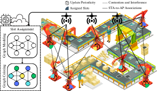
Figure 1: Illustration of a Wi-Fi network for IIoT applications.

In most 802.11 families [9], Wi-Fi devices operate using the carrier-sense multiple access with collision avoidance (CSMA/CA) scheme for channel access, where STAs contend for transmission opportunities [10]. Specifically, to avoid packet collisions with other STAs, an STA waits until the channel is free by sensing ongoing transmissions from other STAs and then backs off for a random time before transmitting its packet to avoid collisions with other STAs also waiting. However, CSMA/CA can cause packet delays and losses due to the following two issues [11]. First, an STA experiences significant backoff time when it senses transmissions from many other STAs, i.e., it contends with numerous surrounding STAs. Second, concurrent transmissions can occur if STAs cannot sense each other’s transmissions due to the large distance between them, which causes inter-STA interference and further decoding errors at the receiving APs. Note that neighboring STAs that trigger backoff or cause interference are referred to as the STA’s contending or hidden neighbors, respectively. Consequently, the native CSMA/CA scheme in Wi-Fi can hardly provide the stringent QoS required by IIoT services due to contention and interference [11].

Recent Wi-Fi 7 standards introduce the restricted target wake time (RTWT) mechanism [12, 13, 14], which allocates exclusive channel access to STAs during specified time slots (or service periods). This approach improves network performance and STAs’ QoS by eliminating contention and interference between STAs in different slots. When applying RTWT, STAs only need to synchronize slot boundaries and avoid frame transmissions across allocated slot boundaries [15]. Due to its relaxed synchronization requirements, RTWT is an attractive candidate for managing contention and interference across large Wi-Fi IIoT networks. Straightforwardly, each STA can be assigned a separate slot to eliminate all contention and interference in the network. However, such a scheme can cause significant delays in large networks, as each STA must wait for the slots of many other STAs to end. STAs can share a slot if their contention is unlikely to disrupt other STAs’ transmissions, or if the interference among them is negligible. Challenges arise in designing a slot assignment scheme that ensures transmission reliability while minimizing the number of slots needed to separate STAs.

I-A Related Works

Several approaches can model contention and interference and design slot assignment schemes in Wi-Fi 7 IIoT networks.

I-A1 Markov Model Approach

The CSMA/CA process in Wi-Fi STAs can be effectively modeled using Markov chains [10, 11], capturing the impact of contention and interference from neighboring STAs. QoS metrics for STAs, such as channel utilization [16] and energy efficiency [17], can be derived from the steady states of these models. However, these Markov models [10, 11] are non-linear and lack closed-form expressions for various STA transmission configurations [18], making them challenging to apply in optimizing slot assignments. Moreover, applying these models requires prior measurements of all contending and hidden STA pairs, resulting in significant network overhead. These limitations reduce the practicality of Markov models in Wi-Fi IIoT networks.

I-A2 Heuristic Graph Model Approach

STA-pairwise contention and interference information can be represented as edges between STAs, forming a graph with STAs as vertices. Slot assignment tasks can then be modeled as graph theory problems [19, 20, 21], such as graph cut [19] or graph coloring [20, 21]. These tasks divide STAs into different slots (either in time or frequency) by disconnecting edges between contending or interfering STA pairs. However, these methods construct graphs—for instance, by assigning edge values between STAs—based on fixed rules predefined according to human intuition about how contention and interference affect STAs’ QoS. As a result, these heuristic graph construction methods lack flexibility and cannot be optimized to meet specific STA QoS requirements.

I-A3 Neural Network Model Approach

In Wi-Fi networks, neural network (NN) models can be flexibly trained to make control decisions based on STAs’ QoS and network data, without requiring explicit contention and interference models [22]. Classic fully connected neural networks (FNNs) have pre-determined input and output dimensions, which limits their scalability to networks of varying sizes [23]. Instead, graph neural networks (GNNs) [24, 25], which are scalable to the graph or the network size, can be applied. GNNs can make decisions by repeatedly aggregating features (network states) of neighboring vertices (or STAs) without being constrained by network size. However, GNNs lose STA-pairwise information during the aggregation of neighboring STAs’ features. This limitation makes them ineffective for tasks where the correlation between each STA pair’s decisions is critical, such as separating STA pairs that are heavily contending or interfering [26, 27]. Additionally, since the minimum number of slots is unknown, it is challenging to design a GNN architecture capable of directly determining each STA’s slot [28, 29].

I-A4 Neural Graph Modeling Approach

NNs can be employed to generate graphs, retaining the graph structure as well as the flexibility to be trained [30, 31]. For example, the authors of [32, 33] use policy gradient (PG) [34] to train NNs that output graphs representing activated devices and transmission links in an integrated sensing and communication system and a cyber-physical power system, respectively, where devices and links are represented as vertices and edges. In Wi-Fi networks, the authors of [35] apply deterministic policy gradient (DPG) [36] to NNs that output a graph model representing STAs as vertices, with contention and interference impacts represented as weighted edges. The graph is cut based on edge weights to partition contending or interfering STAs into a fixed number of slots [35]. However, challenges remain in minimizing slot usage and ensuring reliability in Wi-Fi IIoT networks. Moreover, the above work [35] studies the Wi-Fi networks with limited numbers of devices, e.g., up to tens of devices. Note that the number of possible device pairs grows quadratically when the number of devices increases. How to design the neural graph modeling (NGM) scheme that models the edges in these massive pairs in large Wi-Fi networks requires future research.

I-B Our Contributions

This paper studies the scalable neural graph modeling (ScNeuGM) approach to assign RTWT slots in Wi-Fi 7 networks, e.g., serving periodic IIoT status updates. Our objective is to determine the optimal slot assignments that separate highly contending and interfering STAs, minimizing the number of slots required in each period while ensuring transmission reliability. The network state information used for slot assignments includes path losses from STAs to their nearby APs and the locations of the APs, requiring no additional measurement overheads between STAs. We model the Wi-Fi network as a binary-directed graph, where STAs are represented as vertices and the contention and interference impacts between STAs are represented as binary edges. The coloring scheme of this graph is mapped to the RTWT slot assignment, i.e., STAs are assigned to the same slot if they share the same color, and the chromatic number of the graph is the total number of slots (colors). We formulate the NGM task as training an NGM NN to generate the optimal graph model, i.e., defining the edges connecting STAs, whose coloring scheme minimizes the number of slots while ensuring STAs’ transmission reliability. Two fundamental challenges in the NGM are addressed in our ScNeuGM scheme for large Wi-Fi networks: 1) The absence of explicit STA-pairwise feedback on each generated edge, since the graph’s performance is measured STA-wise (STAs’ reliability) or network-wise (the number of slots); 2) The high computational complexity in the NGM when all STA pairs are processed in training and inference. To avoid acquiring STA-pairwise feedback, an evolution strategy (ES) [37, 38] algorithm is applied to directly adjust the NN parameters without evaluating individual edges. To reduce the complexity, a deep hashing function (DHF) [39] groups likely contending and hidden STA pairs, reducing the processed pairs.

This paper’s contributions are listed as follows.

• To the best of our knowledge, we are the first to formulate the slot minimization problem in the RTWT slot assignment as the NGM task. Unlike GNN models [24, 25], the STA-pairwise information is preserved on the modeled graph edges, indicating whether each STA pair will be separated or not. Moreover, unlike heuristic graph models [19, 20, 21] that construct edges using fixed rules, the proposed scheme flexibly trains NNs to model optimal graphs for specific STA QoS requirements. Further, unlike the previous NGM in Wi-Fi [35] that is only applicable for a fixed number of slots, the proposed one minimizes the number of slots needed to satisfy STA QoS.

• We apply the ES to optimize the NN to return the graph in the NGM in Wi-Fi networks. Existing works [32, 35] use the PG or the DPG to optimize NN parameters, applying the chain rule to compute the gradient of the graph’s performance w.r.t. the edge values, followed by the gradient of the edge values w.r.t. the NN parameters. Unlike these methods [32, 35], the proposed ES directly adjusts the NN parameters based on the graph’s performance, i.e., STAs’ reliability and the number of slots, without estimating edges’ gradient. The NN trained by the ES is $4$-$10$ times more likely to return near-optimal graphs compared to those trained by the PG or the DPG.

• Also, we apply the DHF to reduce the NGM complexity by focusing on the training and inference within contending or hidden STA pairs in Wi-Fi networks. To identify contending and hidden pairs, the DHF embeds each STA state into a hash code, where the bits of two STAs’ codes are likely equal if they form a contending or hidden pair. By querying random bits in the STAs’ codes, two STAs are grouped if their bits are likely equal, i.e., they are likely contending or hidden pairs. In large networks with $1000$ STAs, the DHF reduces the training and inference time of the NGM by up to $4$ and $8$ times, respectively, and the online slot assignment time by up to $3$ times.

• We implement and deploy the ScNeuGM scheme in a system-level, standard-compliant Wi-Fi simulation platform, NS-3 [40], with RTWT enabled. Simulation results show that the graph returned by the ES-trained NN reduces the number of slots by $25\%$ compared to heuristic graphs designed based on human intuition. Further, in scenarios with mobile STAs, the ScNeuGM achieves up to $30\%$ fewer packet losses by applying the DHF to efficiently group STA pairs, enabling timely graph regeneration to adapt to network dynamics compared to the scheme that processes all STA pairs non-selectively.

I-C Notation and Paper Organization

The $i$-th element of a vector $\mathbf{x}$ is denoted as $x_{i}$. The $j$-th element of the $i$-th row of a matrix $\mathbf{X}$ is denoted as $X_{i,j}$. We define the elements of $\mathbf{X}$ as $\mathbf{X}\triangleq[X_{i,j}\mid X_{i,j}=(\cdot)]$, where $(\cdot)$ represents the expression defining $\mathbf{X}$’s elements. $\operatorname{\bf diag}{\mathbf{X}}$ denotes the diagonal elements of $\mathbf{X}$. $\mathbf{1}_{\{\cdot\}}$ is an indicator that equals $1$ if $\{\cdot\}$ is true and $0$ otherwise. $\land$ is logical AND.

The rest of this paper is organized as follows. Section II presents the system model. Section III defines the NGM task for contention and interference management and explains the overall concept of the ScNeuGM framework. Sections IV and V present the ES and the DHF in the ScNeuGM, respectively. Finally, Section VI shows the simulations evaluating the proposed methods, and Section VII concludes this work.

II System Model

This section presents the system model of the Wi-Fi network, including the network configurations, the RTWT mechanism, and the network state information.

II-A Wi-Fi Network Configurations

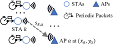
Figure 2: System model of the Wi-Fi IIoT network.

In the network, STAs are assumed to be sensors or monitors continuously collecting data to track critical information in IIoT applications, such as manufacturing systems, and transmitting the collected data samples to the APs via the uplink, as shown in Fig. 1. We consider a Wi-Fi network consisting of $K$ STAs and $A$ APs, as illustrated in Fig. 2. The APs are located in a two-dimensional space, and each AP’s location is known in advance as $\mathrm{loc}_{a}\triangleq(x_{a},y_{a})$, where $x_{a}$ and $y_{a}$ are the coordinates of AP $a$ along the $x$ and $y$ axes, respectively, with $a=1,\dots,A$. All STAs and APs are assumed to operate on the same channel with a bandwidth $B$ in Hertz (Hz). The transmission power of the STAs is $\mathbf{P}_{\mathrm{0}}$ in milliwatts (mW), and the noise power spectral density is $\mathbb{N}_{\mathrm{0}}$ in mW/Hz. The path loss from STA $k$ to AP $a$ is denoted as $s_{k,a}$ in dB, $\forall k,a$. Each STA is associated with the AP that has the minimum path loss to the STA, and the associated AP receives and collects the STA’s transmitted packets. We denote the associated AP of STA $k$ as $\hat{a}_{k}$, i.e.,

$$\hat{a}_{k}\triangleq\arg\min_{a}s_{k,a},\ \forall k.$$ (1)

We assume that the same data-collection mechanism is used in all STAs over time and that STAs encapsulate each collected data sample into a packet with a constant format, i.e., each STA has the same packet arrival process with a packet size of $L$ bits. Let $d_{k}$ (in seconds) denote the transmission duration of an $L$-bit packet for STA $k$, which depends on the modulation and coding scheme (MCS). Each STA’s MCS is configured to be the highest one for which the decoding error probability without interference, $\epsilon_{k}$, is below a threshold $\epsilon_{\max}=10^{-5}$. The decoding error probability $\epsilon_{k}$ for short packets can be approximated as [41]

$$\epsilon_{k}\approx f_{Q}\Bigg{(}\frac{-L\ln{2}+{d_{k}B}\ln(1+\phi_{k})}{\sqrt{d_{k}BV}}\Bigg{)},\ \forall k,$$ (2)

where $\phi_{k}=(\mathbf{P}_{\mathrm{0}}/s_{k,\hat{a}_{k}})/(\mathbb{N}_{\mathrm{0}}B)$ is the signal-to-noise-ratio (SNR) of STA $k$ without interference ($s_{k,\hat{a}_{k}}$ here is converted to the decimal scale). In (2), $f_{Q}$ is the tail distribution of the standard normal distribution, and $V$ is the channel dispersion as $V=1-{1}/{\big{[}1+\phi_{k}\big{]}^{2}}$ [41] in (2). Note that we assume that $\mathbf{P}_{\mathrm{0}}$, $\mathbb{N}_{\mathrm{0}}$, $B$, and $L$ in (2) are constants in the network, Thus, for each STA $k$, the packet durations $d_{k}$ only depends on the path loss to STAs’ associated APs, $s_{k,\hat{a}_{k}}$, $\forall k$.

II-B CSMA/CA with RTWT

We assume that all STAs and APs are synchronized in time, and the time is divided into slots indexed by $t$, where $t=1,2,\dots$. The duration of each slot is denoted as $\Delta_{\mathrm{0}}$ seconds. The network assigns a periodic slot $z_{k}$ to STA $k$ as its RTWT service period, where the same periodicity $Z$ is configured across all STAs in the network. The periodicity $Z$ directly affects the freshness of status updates from STAs. A higher value of $Z$ increases delays in status updates, whereas a lower value of $Z$ results in more STAs sharing the same slots, leading to contention and interference that can degrade transmission reliability. Specifically, STA $k$, for $k=1,\dots,K$, is scheduled to transmit exclusively during the periodic time slots $t=z_{k},z_{k}+Z,z_{k}+2Z,\dots$. Here, two STAs $i$ and $j$ transmit in the same slot if $z_{i}=z_{j}$, $\forall i,j$. For example, as shown in Fig. 3, three STAs ($K=3$) are assigned two slots within one RTWT period ($Z=2$). The illustrated case eliminates contention and interference between STAs $2$ and $1$ as well as between STAs $2$ and $3$, while contention and interference may occur between STAs $1$ and $3$.

In the allocated slot, each STA contends for channel access using CSMA/CA [9] when its assigned slots start periodically. In each assigned slot, the STA first checks whether any other STA is transmitting on the channel. If the channel is busy, the STA continues monitoring it until it becomes idle. Once the channel is idle, the STA initiates a random backoff period to further reduce the probability of collision with other STAs waiting to transmit. If the channel becomes busy during the backoff period, the countdown is paused and resumes once the channel is idle again. After the backoff period ends, the STA transmits one packet. If some STAs cannot sense this transmission (i.e., they are hidden from each other), simultaneous transmissions may occur, causing interference at the receiving AP and increasing the decoding error probability. The AP sends a negative acknowledgment if the packet transmission fails, triggering the STA to retransmit the same packet. Retransmission repeats until the maximum number of attempts is reached or an acknowledgment is received. Afterward, the STA waits for the next assigned slot in the subsequent period.

Due to contention from neighboring STAs, each STA may experience a significant backoff time, delaying the packet transmission to the later part of the slot. In this case, if transmitting the packet would occupy the channel beyond the ending time of the assigned slot, the STA skips the packet transmission in this slot and waits for the next assigned slot in the following period. Consequently, each STA contends and interferes only with those STAs that have the same assigned slots, while contention and interference are eliminated between STAs with different assigned slots.

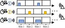
Figure 3: Illustration of the slot assignments for $K=3$ STAs with $Z=2$ slots, where STA $1$ and $3$ are assigned in the same slot, e.g., $z_{1}=z_{3}=1$, and STA $2$ is assigned with a different one, e.g., $z_{2}=2$.

II-C Wi-Fi Network States

We next explain the network state information that will be used in the proposed slot assignment scheme.

II-C1 Measured Network States

We assume that Wi-Fi devices have practical receiver sensitivities. In other words, if the path loss (in dB) between a STA and an AP exceeds a threshold $s_{\max}$ (in dB), the STA’s transmissions cannot be detected or received by the AP. Consequently, this path loss cannot be measured from the network. For a given $k$-th STA, where $k=1,\dots,K$, we collect and sort the APs that can detect the STA’s signal into a list as

$$\mathcal{A}_{k}\triangleq\{a_{k}(1),a_{k}(2),\dots,a_{k}(|\mathcal{A}_{k}|)\},\ \forall k\ ,$$ (3)

where $s_{k,a}\leq s_{\max},\ \forall a\in\mathcal{A}_{k}$, and $|\mathcal{A}_{k}|$ denotes the number of APs capable of detecting STA $k$’s signal. The APs in (3) are sorted in ascending order of path loss from STA $k$, such that $s_{k,a_{k}(i)}\leq s_{k,a_{k}(j)},\ \forall i<j$. Clearly, $a_{k}(1)=\hat{a}_{k}$, as $a_{k}(1)$ represents the AP with the minimum path loss to STA $k$, and STA $k$ is associated with this AP, as mentioned in Section II-A. We denote STA $k$’s path loss to an AP in the above list, along with the location of the AP, as a state vector:

$$\mathbf{s}_{k}(i)\triangleq[s_{k,a_{k}(i)},x_{a_{k}(i)},y_{a_{k}(i)}]^{\rm T},\ i=1,\dots,|\mathcal{A}_{k}|,\ \forall k.$$ (4)

The sequence of sorted STA $k$’s state vectors is written as

$$\mathcal{S}_{k}\triangleq\{\mathbf{s}_{k}(1),\mathbf{s}_{k}(2),\dots,\mathbf{s}_{k}(|\mathcal{A}_{k}|)\},\ \forall k,$$ (5)

Finally, the collection of all such sequences is defined as

$$\hat{\mathcal{S}}\triangleq\{\mathcal{S}_{1},\dots,\mathcal{S}_{K}\}.$$ (6)

We refer to $\hat{\mathcal{S}}$ as the network states and $\mathcal{S}_{k}$ as STA $k$’s state, where $k=1,\dots,K$. Note that the size of each STA’s state, $\mathcal{S}_{k}$, may vary since STAs can have different numbers of APs capable of detecting their signals, depending on the locations of the STAs and APs. Here, $\hat{\mathcal{S}}$ represents the measured network states and serves as the input to the proposed methods.

II-C2 Unmeasured Network States

Whether a pair of STAs is a contending or hidden pair significantly impacts their channel access and transmission reliability [11]. Contending and hidden STAs depend on the path losses between STA pairs, specifically on whether two STAs can detect each other. Measuring the path losses for all $K$ STAs requires approximately $\mathcal{O}(K^{2})$ measurements for all STA pairs, which introduces significant overhead to the network. Therefore, we assume that contending and hidden STA relationships are not measured during the online deployment of the proposed methods but are instead used as training information in offline simulations. Specifically, contending and hidden STA pairs are represented by binary indicators as

$$O^{\mathrm{C}}_{i,j}\triangleq\mathbf{1}_{\{l(i,j)\leq\hat{l}\}};\ O^{\mathrm{H}}_{i,j}\triangleq\mathbf{1}_{\{l(i,j)>\hat{l}\}}\land\mathbf{1}_{\{s_{i,\hat{a}_{j}}\leq s_{\max}\}},\ \forall i,j.$$ (7)

We set $O^{\mathrm{C}}_{i,j}=1$ if the distance $l(i,j)$ between STAs $i$ and $j$ is in the detectable range $\hat{l}$ of STA $j$, indicating STA $i$ is contending $j$, and set $O^{\mathrm{H}}_{i,j}=1$ if STA $i$ is not in the detectable range $\hat{l}$ of STA $j$ and STA $i$ interferes with STA $j$’s AP, i.e., STA $i$ is hidden from STA $j$. $O^{\mathrm{C}}_{i,j}+O^{\mathrm{H}}_{i,j}$ denotes that a STA pair $(i,j)$ is either contending or hidden STAs. We assume that if two STAs are neither contending nor hidden STAs, their transmissions do not affect each other.

III ScNeuGM Framework for Contention and Interference Management

This section begins by defining the QoS requirements of the STAs and formulating the RTWT slot assignment problem to manage contention and interference. Subsequently, the problem is transformed into a graph modeling task, where optimizing the edge values in the graph corresponds to optimizing its coloring scheme, which further optimizes the slot assignment. Finally, we present the ScNeuGM framework that trains the NN generating the optimal graph, highlighting the challenges posed in large networks.

III-A Contention and Interference Management Using RTWT

To improve QoS and reduce packet loss rates, we assign the slot choices of STAs $\mathbf{z}\triangleq[z_{1},\dots,z_{K}]$ in the period, where $z_{k}\in\{1,\dots,Z\}$ $\forall k$. Let $u_{k}(n)$ denote the number of packets successfully sent by STA $k$ during the $n$-th period, where $n=1,2,3,\dots$, and $u_{k}(n)\in\{0,1\}$ since each STA transmits only one packet per period, as mentioned in Section II. The reliability of each STA is defined as the successful packet transmission rate averaged over time as

$$r_{k} \triangleq\lim_{N\to\infty}\frac{1}{N}\sum_{n=1}^{N}u_{k}(n),\ \forall k.$$ (8)

Note that unsuccessful transmissions can occur due to insufficient transmission time in each assigned slot (e.g., caused by contention backoffs) or due to decoding errors (e.g., caused by interference). The QoS requirement is that each STA’s reliability must exceed a threshold $\hat{r}$. We express the expected value of the reliability of STA $k$ for given measured network states and slot assignment decisions as $\operatorname{\mathbb{E}}[r_{k}|\hat{\mathcal{S}},\mathbf{z}]$. The objective is to minimize the number of slots, $Z$, in the period or equivalently the transmission periodicity while ensuring transmission reliability as

$$\min_{\mathbf{z},Z}\ Z,\ \text{s.t. }\operatorname{\mathbb{E}}[r_{k}|\hat{\mathcal{S}},\mathbf{z}]\geq\hat{r},\ z_{k}\in\{1,\dots,Z\},\ \forall k.$$ (9)

The straightforward formulation in (9) is challenging to solve due to the lack of a clear structure for deriving the slot assignments and the minimum slot number from the network states. To address this issue, the problem is transformed into a graph modeling task, as described below.

III-B Problem Transformation to Graph Modeling Task

In Wi-Fi networks, contention and interference are pairwise interactions between STAs. To effectively represent these STA-pairwise interactions, we model the network as a binary-directed graph, $\mathcal{G}=(\mathcal{V},\mathcal{E})$, where the STAs are vertices $\mathcal{V}$ and each directed edge $(i,j)\in\mathcal{E}$ implies that STA $i$’s transmissions will cause a QoS violation for STA $j$’s transmissions if they are in the same slot. The adjacency matrix $\mathbf{E}$ of $\mathcal{G}$ is defined with binary edges as

$$\mathbf{E}\triangleq\big{[}E_{i,j}\big{|}E_{i,j}\in\{0,1\},\ \forall i\neq j;\ E_{k,k}=0,\ \forall k\big{]}.$$ (10)

Graph coloring is employed to assign colors to vertices (STAs) such that no two adjacent vertices share the same color. Each color represents a distinct group of STAs that can transmit simultaneously without causing QoS violations, i.e., they can be assigned to the same slot. If an edge $(i,j)$ exists (i.e., $E_{i,j}=1$), STAs $i$ and $j$ must be assigned different colors to avoid contention and interference. We denote the coloring scheme of the binary graph with adjacency matrix $\mathbf{E}$ as

$$\mathbf{z}^{\prime},Z^{\prime}=\chi(\mathbf{E}).$$ (11)

Here, $\mathbf{z}^{\prime}=[z^{\prime}_{1},\dots,z^{\prime}_{K}]^{\rm T}$ represents the proper color choices for STAs $1,\dots,K$ that satisfy the edge constraints on the graph, and $Z^{\prime}$ denotes the minimum number of colors required to color the graph (i.e., the graph’s chromatic number), where $z^{\prime}_{k}\in\{1,\dots,Z^{\prime}\}$ $\forall k$. The coloring scheme is mapped to the slot assignments as follows.

Proposition 1.

There exists an adjacency matrix $\mathbf{E}^{*}$ of the graph whose coloring scheme, $\mathbf{z}^{*},Z^{*}=\chi(\mathbf{E}^{*})$, solves the contention and interference management problem in (9). In other words, $\mathbf{z}^{*}$ and $Z^{*}$ represent the optimal slot assignments in (9), minimizing the number of slots while satisfying the STAs’ reliability constraints.

Proof.

The proof is in the appendix. ∎

Therefore, by optimizing the graph’s binary edge values and then coloring the graph, we can equivalently optimize the slot assignments in the problem (9). Based on this fact, we construct the following graph modeling optimization task as

$$\min_{E_{i,j}\in\{0,1\},\forall i\neq j}\ Z,\ \textrm{s.t.} \operatorname{\mathbb{E}}[r_{k}|\hat{\mathcal{S}},\mathbf{z}]\geq\hat{r},\ \forall k,$$ (12)

$$\mathbf{z},Z=\chi(\mathbf{E}),$$

where the graph coloring in (11) is embedded to decide the STAs’ slots and the edge values of the graph are optimized instead. Since there exists an optimal graph whose coloring scheme is the optimal slot assignment, as shown in Proposition 1, we can find the optimal slot assignments in (9) by solving the problem (12) instead. As a result, this formulation in (12) transforms the slot assignment problem into a graph modeling task that finds the optimal binary graph representing the impact of the contention and interference on STAs’ transmissions.

III-C Neural Graph Modeling

Note that the optimal graph model is unknown and is difficult to derive analytically due to the complex interactions among STAs. Therefore, we simplify the problem by assuming that each binary edge value in the optimal graph, $E^{*}_{i,j}$, is a function of the states of STA $i$ and STA $j$, $\mathcal{S}_{i}$ and $\mathcal{S}_{j}$, as

$$E^{*}_{i,j}\triangleq\mu^{*}(\mathcal{S}_{i},\mathcal{S}_{j}),\ \forall i\neq j,$$ (13)

where we refer to $\mu^{*}(\cdot)$ as the optimal graph modeling function, mapping each STA pair’s states to the optimal edge value between them. This assumption further transforms the slot assignment task into the problem of finding the optimal graph modeling function $\mu^{*}(\cdot)$. Note that such a function can be heuristically designed based on human intuition, e.g., using the network state information as $\mu^{*}(\mathcal{S}_{i},\mathcal{S}_{j})\approx\mathbf{1}_{\{\mathcal{A}_{i}\cap\mathcal{A}_{j}\neq\emptyset\}},\forall i,j$ [21], where $\mathcal{A}_{i},\forall i$ can be computed using $\mathcal{S}_{i}$ as (3). However, heuristic designs rely on a fixed function and therefore cannot be adjusted to optimally capture the impact of contention and interference on STAs’ reliability or minimize the number of slots. This issue can be addressed by approximating the unknown structure of $\mu^{*}(\cdot)$ using a NN [35], as

$$E_{i,j}=\mu(\mathcal{S}_{i},\mathcal{S}_{j}|\theta^{\mu})\approx\mu^{*}(\mathcal{S}_{i},\mathcal{S}_{j}),\ \forall i\neq j,$$ (14)

where $\theta^{\mu}$ denotes $\mu(\cdot)$’s parameters that can be flexibly trained using machine learning (ML). We refer to $\mu(\cdot|\theta^{\mu})$ as the NGM NN for Wi-Fi contention and interference management.

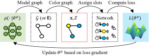
Figure 4: Iterative training of the NGM NN $\mu(\cdot|\theta^{\mu})$ for the contention and interference management problem in the Wi-Fi network.

Fig. 4 illustrates the iterative training of the NGM NN for managing contention and interference. The process begins with the NGM NN, $\mu(\cdot|\theta^{\mu})$, computing the edge values $\mathbf{E}$ between STA pairs to generate the binary graph model $\mathcal{G}$. This graph is then colored to obtain the slot assignment decision, $\mathbf{z}$ and $Z$. The network evaluates the performance of the decision and computes the loss, $L(\theta^{\mu})$, on the NN parameters $\theta^{\mu}$. Finally, the NN parameters $\theta^{\mu}$ are updated based on the loss value using the ML algorithm, and the workflow repeats until the NN is optimized. Note that graph coloring is an NP-hard task. To perform graph coloring efficiently with low complexity, we employ a greedy coloring scheme [42] that prioritizes STAs with higher degrees. Meanwhile, designing coloring algorithms is beyond the scope of this work.

III-D Overview of ScNeuGM Framework

When scaling the NGM to a large network with a significant number of Wi-Fi devices, several issues arise due to the massive amount of STA pairs, negatively impacting the NGM performance. The ScNeuGM framework addresses them accordingly as follows.

III-D1 Implicit Loss on Edge Values

In the iteration of the NGM training, the NN parameters $\theta^{\mu}$ are updated in the direction of minimizing the loss $L(\theta^{\mu})$, i.e., the gradient of the loss w.r.t. the parameters, $-\nabla_{\theta^{\mu}}L(\theta^{\mu})$. Typically, this gradient is estimated using the chain rule [32, 35], which decomposes into the gradient of the loss w.r.t. each edge value and the gradient of the edge value w.r.t. the NN parameters, e.g.,

$$-\nabla_{\theta^{\mu}}L(\theta^{\mu})=-\nabla_{\mathbf{E}}L(\theta^{\mu})\nabla_{\mathbf{\theta^{\mu}}}\mathbf{E}=-\sum_{i\neq j}\frac{\partial L(\theta^{\mu})}{\partial E_{i,j}}\nabla_{\mathbf{\theta^{\mu}}}E_{i,j}.$$ (15)

However, the partial derivative of the loss w.r.t. each edge value, $\partial L(\theta^{\mu})/\partial E_{i,j}$, can hardly be explicitly estimated. This is because the graph’s performance is measured either STA-wise (e.g., each STA’s reliability) or network-wide (e.g., the number of slots used), and there is no edge-wise (or STA-pairwise) feedback. Meanwhile, the graph’s performance is highly sensitive to individual edge values. For example, if an STA pair is heavily contending or interfering with each other but the NGM NN fails to set $1$ on the edge between them, the reliability constraints of the STAs could be violated. Conversely, if the NGM NN sets $1$ on edges between non-contending and non-hidden STAs, the chromatic number of the graph will increase, preventing the minimization of the number of slots. Due to the implicit nature of STA-pairwise feedback and the performance’s sensitivity to individual edge values, edge gradient estimation in (15) fails to provide efficient update directions for the NGM NN parameters. To address this issue, ScNeuGM uses the ES algorithm, an edge-feedback-free method, for estimating the update directions of the NGM NN in Section IV.

III-D2 Quadratic Complexity In Network Size

The number of possible STA pairs in the network grows quadratically with the number of STAs. For instance, in a network with one thousand STAs, there would be one million STA pairs. Simulating the interactions and computing the edges between all pairs will cause a significant computational load in large networks. The computation can be intuitively accelerated by computing edges only between contending or hidden STA pairs, which is formally stated as

Theorem 1.

For any optimal graph $\mathcal{G}^{*}$, the graph $\mathcal{G}^{\prime}$ with edges defined as $E^{\prime}_{i,j}=E^{*}_{i,j}\land(O^{\mathrm{C}}_{i,j}+O^{\mathrm{H}}_{i,j})$ is also optimal. Here, $O^{\mathrm{C}}_{i,j}+O^{\mathrm{H}}_{i,j}$ indicates whether STAs $i$ and $j$ are contending or hidden, as defined in Section II.

Proof.

The proof is in the appendix. ∎

The above statement implies that any optimal graph remains optimal if edges between non-contending and non-hidden STA pairs are removed. It further suggests that the NGM only needs to consider the edges for contending and hidden pairs, while the remaining edges can be ignored and set to $0$. However, since the indicators of contending and hidden pairs, $O^{\mathrm{C}}_{i,j}$ and $O^{\mathrm{H}}_{i,j}$ $\forall i,j$, are not measured, it is unknown which STA pairs require the NGM operations. To address this issue, ScNeuGM uses a low-complexity method based on the DHF to efficiently select the contending and hidden STA pairs in Section V.

IV Parameter Space Optimization of NGM NN Using Evolution Strategy

This section first presents the structure of the NGM NN, followed by the ES algorithm training the NN in the ScNeuGM.

IV-A Design of NGM NN Structure

The structure of the NGM NN $\mu(\cdot|\theta^{\mu})$ is shown in Fig. 5, consisting of 1) a state embedding that maps the STA state sequences in (3) into fixed-dimensional embedding vectors, 2) predictors that infer contention and interference between STA pairs, and 3) an edge generator that outputs the binary edge value. The design of each component is explained as follows.

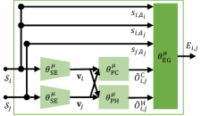
Figure 5: The structure of the NGM NN $\mu(\cdot|\theta^{\mu})$. Here, the state embedding with parameters $\theta^{\mu}_{\mathrm{SE}}$, the predictors with parameters $\theta^{\mu}_{\mathrm{PC}}$ and $\theta^{\mu}_{\mathrm{PH}}$ are trained using unsupervised/supervised learning in the appendix, and the edge generator with parameters $\theta^{\mu}_{\mathrm{EG}}$ are trained using the ES in Algorithm 2.

IV-A1 State Embedding

We design the state embedding NN (SENN) as an autoencoder [43] that embeds the STA state sequences into a vector. To embed the sequence, multi-layer long short-term memory (LSTM) NNs are employed to construct the encoder [44]. Specifically, the $\mathrm{SENN}(\cdot|\theta^{\mu}_{\mathrm{SE}})$, with parameters $\theta^{\mu}_{\mathrm{SE}}$, computes each STA’s embedding vector as

$$\mathbf{v}_{k}=\mathrm{SENN}(\mathcal{S}_{k}|\theta^{\mu}_{\mathrm{SE}}),\ \forall k,$$ (16)

where internally LSTMs generate the embedding vector as

$$\mathbf{h}_{a}^{(l)},\mathbf{c}_{a}^{(l)}=\mathrm{LSTM}^{(l)}(\mathbf{h}_{a}^{(l-1)},\mathbf{h}_{a-1}^{(l)},\mathbf{c}_{a-1}^{(l)}|\theta^{\mu}_{\mathrm{SE}}),\ \forall l,a.$$ (17)

where $l=1,\dots,\xi$ is the layer index and $a=1,\dots,|\mathcal{A}_{k}|$ is the position index in the sequence $\mathcal{S}_{k}$. Here, $\mathbf{h}_{a}^{(l)}$ and $\mathbf{c}_{a}^{(l)}$ are the hidden and cell vectors in the $(l,a)$-th LSTM block, $\forall l,a$. The initial hidden state is set as $\mathbf{h}_{0}^{(l)}=\mathbf{0}$ for $\forall l$. The input to the first layer, $\mathbf{h}_{a}^{(0)}=\mathbf{s}_{k}(a)$ for $a\geq 1$, represents the $a$-th AP information in $\mathcal{S}_{k}$. The embedding vector is defined as the hidden state vector of the last block in the last layer, i.e., $\mathbf{v}_{k}=\mathbf{h}_{|\mathcal{A}_{k}|}^{(\xi)}|_{\mathrm{SENN}(\mathcal{S}_{k}|\theta^{\mu}_{\mathrm{SE}})}$. Note that in the SENN, we use FNNs to embed the input and output. The notations of these FNNs are simplified from the above LSTM expressions, and their structures will be explained in Section VI.

IV-A2 Contention and Interference Predictors

Using STA embedding vectors, we can predict how likely each STA pair is contending or hidden using NNs, which assists in deciding edge values. For instance, we use two fully connected NNs, the PCNN and the PHNN, to predict the indicators of contenting and hidden pairs, $O^{\mathrm{C}}_{i,j}$ and $O^{\mathrm{H}}_{i,j}$, based on the embedding vectors $\mathbf{v}_{i}$ and $\mathbf{v}_{j}$ as

$$\tilde{O}^{\mathrm{C}}_{i,j}=\mathrm{PCNN}(\mathbf{v}_{i},\mathbf{v}_{j}|\theta^{\mu}_{\mathrm{PC}});\ \tilde{O}^{\mathrm{H}}_{i,j}=\mathrm{PHNN}(\mathbf{v}_{i},\mathbf{v}_{j}|\theta^{\mu}_{\mathrm{PH}}),$$ (18)

where $\tilde{O}^{\mathrm{C}}_{i,j}$ and $\tilde{O}^{\mathrm{H}}_{i,j}$ are the predicted values of $O^{\mathrm{C}}_{i,j}$ and $O^{\mathrm{H}}_{i,j}$, respectively, $\forall i\neq j$.

IV-A3 Edge Generator

We extract key information on contention and interference to assist the NGM NN in deciding edge values. Specifically, for a given STA pair $i$ and $j$ (where $i\neq j$), the edge value $E_{i,j}$ is generated based on the following information in $\mathcal{S}_{i}$ and $\mathcal{S}_{j}$, representing the negative impact of STA $i$’s transmissions on those of STA $j$ [35], as

• $s_{i,\hat{a}_{i}}$: Path loss from STA $i$ to its associated AP $\hat{a}_{i}$, which determines the packet duration of STA $i$, i.e., the interference duration caused by STA $i$. A smaller $s_{i,\hat{a}_{i}}$ results in shorter interference durations from STA $i$.

• $s_{i,\hat{a}_{j}}$: Path loss from STA $i$ to STA $j$’s AP $\hat{a}_{j}$. It indicates the interference power at the AP. A smaller $s_{i,\hat{a}_{j}}$ indicates higher interference from STA $i$ to STA $j$’s transmissions.

• $s_{j,\hat{a}_{j}}$: Path loss from STA $j$ to its associated AP $\hat{a}_{j}$. It determines STA $j$’s received signal power and packet duration. A smaller $s_{j,\hat{a}_{j}}$ indicates a shorter packet duration and a stronger signal, making STA $j$’s transmissions more robust against contention and interference.

• $\tilde{O}^{\mathrm{C}}_{i,j}$ and $\tilde{O}^{\mathrm{H}}_{i,j}$: Probabilities of the STA pair being contending or hidden, predicted based on their state embeddings. When determining $E_{i,j}$, edge value generation integrates these probabilities with $s_{i,\hat{a}_{i}}$, $s_{j,\hat{a}_{j}}$, and $s_{i,\hat{a}_{j}}$.

We design the edge generator NN (EGNN) based on the extracted contention and interference information as

$$E_{i,j}=\mathrm{EGNN}(s_{i,\hat{a}_{i}},s_{i,\hat{a}_{j}},s_{j,\hat{a}_{j}},\tilde{O}^{\mathrm{C}}_{i,j},\tilde{O}^{\mathrm{H}}_{i,j}|\theta^{\mu}_{\mathrm{EG}}),\ \forall i\neq j.$$ (19)

Note that the EGNN is configured to output a value in $[0,1]$, where the edge value is rounded to the nearest integer, $0$ or $1$, without explicit notation for simplicity.

In summary, the NGM NN parameters consist of the SENN parameters $\theta^{\mu}_{\mathrm{SE}}$, the predictor parameters $\theta^{\mu}_{\mathrm{PC}}$ and $\theta^{\mu}_{\mathrm{PH}}$, and the edge generator parameters $\theta^{\mu}_{\mathrm{EG}}$. When generating the edge for an STA pair $(i,j)$, $\forall i\neq j$, the NGM NN first embeds the STA states $\mathcal{S}_{i}$ and $\mathcal{S}_{j}$ using the SENN as in (16). It then predicts the contention and interference indicators based on the embeddings using the PCNN and the PHNN as in (18), and finally generates the edge using the EGNN as in (19).

IV-B Evolution Strategy for Training the NGM NN

Since the ES algorithm is a parameter space algorithm, we pre-train some parts of the NGM NN to reduce the number of parameters of the NN to be trained by the ES. Specifically, the state embedding and the predictors are pre-trained using unsupervised learning and supervised learning, respectively, as shown in the appendix. Consequently, these parameters in the NGM NN are fixed after pre-training, while only the parameters in the EGNN are updated by the ES. The detailed implementation of the ES is presented as follows.

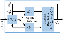
Figure 6: The ES algorithm that trains the EGNN in the NGM NN.

IV-B1 Reward Design

We aggregate the STAs’ reliability and the number of slots into one reward signal. Specifically, we augment the reliability definition as the number of packets transmitted within the minimum number of slots. For example, if the number of slots $Z$ obtained by coloring the graph exceeds the minimum $Z^{*}$, we can emulate an imaginary system that randomly selects STAs assigned to the $Z^{*}$ slots out of the total $Z$ slots to transmit, while STAs’ transmissions in other slots are discarded. Consequently, the augmented reliability is expressed in the log scale as

$$R=\begin{cases}\log(\frac{Z^{*}}{Z}),\ \text{if }r_{k}\geq\hat{r},\ \forall k\ ,\\ \log(\min\{\frac{Z^{*}}{Z},1\}\cdot\frac{1}{K}\sum_{k=1}^{K}\min\{\frac{r_{k}}{\hat{r}},1\}),\ \text{otherwise}.\end{cases}$$ (20)

If the reliability constraints are satisfied, the reward focuses on minimizing the number of slots; otherwise, the reward emphasizes satisfying the reliability constraints. The maximum reward signal in (20) is 0, and it is achieved if and only if the slot assignments minimize the number of slots while ensuring STA reliability. Note that the minimum number of slots $Z^{*}$ is unknown. Thus, we use the chromatic number of the contention and interference graph, with edges defined as $(O^{\mathrm{C}}_{i,j}+O^{\mathrm{H}}_{i,j})$ for $i\neq j$, as an approximation of $Z^{*}$. To normalize the reward signal, we measure the average reward over the iterations as $\bar{R}$ and aim to maximize the advantage [42, 45] of the reward with respect to the past average, as $R-\bar{R}$. Therefore, the loss of the EGNN parameters in the NGM is designed as

$$L(\theta^{\mu}_{\mathrm{EG}})=-\operatorname{\mathbb{E}}[R-\bar{R}].$$ (21)

IV-B2 Parameter Space Update

We optimize the EGNN parameters using a Gaussian ES algorithm [38]. In the ES algorithm, each parameter of the EGNN is assumed to be a Gaussian random variable, independent of each other, with the mean $m^{\mu}_{\mathrm{EG}}$ and the variance $\exp({\nu^{\mu}_{\mathrm{EG}}})$. Here, the exponential ensures the variance is always positive. The ES algorithm adjusts each parameter’s mean and variance to find the optimal values that maximize the reward signal, as shown in Fig. 6. Specifically, it first randomly samples parameters $\tilde{\theta}^{\mu}_{\mathrm{EG}}$ from the current distribution as

$$\tilde{\theta}^{\mu}_{\mathrm{EG}}\sim\mathcal{N}(m^{\mu}_{\mathrm{EG}},\exp({\nu^{\mu}_{\mathrm{EG}}})).$$ (22)

Using the sampled EGNN parameters $\tilde{\theta}^{\mu}_{\mathrm{EG}}$, the NGM NN generates the edges in the graph based on the network states $\hat{\mathcal{S}}$, as described in Section IV-A. The instant reward, $\dot{R}$, is then evaluated as (20) from the network based on the corresponding slot assignments by coloring the graph. The gradient of the loss function with respect to the parameterized distribution (the mean and the variance) of the EGNN parameters is

$$-\nabla_{m^{\mu}_{\mathrm{EG}},\nu^{\mu}_{\mathrm{EG}}}L(\theta^{\mu}_{\mathrm{EG}})=\nabla_{m^{\mu}_{\mathrm{EG}},\nu^{\mu}_{\mathrm{EG}}}\operatorname{\mathbb{E}}\big{[}R-\bar{R}\big{]}$$ (23)

$$\stackrel{{\scriptstyle\text{(a)}}}{{=}}\operatorname{\mathbb{E}}_{\theta^{\mu}_{\mathrm{EG}}\sim\mathcal{N}(m^{\mu}_{\mathrm{EG}},\exp({\nu^{\mu}_{\mathrm{EG}}}))}\big{[}(R-\bar{R})\nabla_{m^{\mu}_{\mathrm{EG}},\nu^{\mu}_{\mathrm{EG}}}\log p(\theta^{\mu}_{\mathrm{EG}})\big{]}$$

$$\stackrel{{\scriptstyle\text{(b)}}}{{\approx}}(\dot{R}-\bar{R})\nabla_{m^{\mu}_{\mathrm{EG}},\nu^{\mu}_{\mathrm{EG}}}\log p(\tilde{\theta}^{\mu}_{\mathrm{EG}})\ ,$$

where $p(\cdot)$ is the probability density function of the EGNN parameters, i.e., the Gaussian distribution with mean $m^{\mu}_{\mathrm{EG}}$ and variance $\exp({\nu^{\mu}_{\mathrm{EG}}})$. Here, (a) uses the log-derivative trick to move the gradient computation into the expectation [34], and (b) is the approximation of the expected gradient in the current iteration. By further substituting the expression for the Gaussian distribution’s probability density function, we have

$$-\nabla_{m^{\mu}_{\mathrm{EG}}}L(\theta^{\mu}_{\mathrm{EG}}) \approx(\dot{R}-\bar{R})\cdot\frac{\tilde{\theta}^{\mu}_{\mathrm{EG}}-m^{\mu}_{\mathrm{EG}}}{\exp({\nu^{\mu}_{\mathrm{EG}}})};$$ (24)

$$-\nabla_{\nu^{\mu}_{\mathrm{EG}}}L(\theta^{\mu}_{\mathrm{EG}}) \approx(\dot{R}-\bar{R})\cdot(\frac{(\tilde{\theta}^{\mu}_{\mathrm{EG}}-m^{\mu}_{\mathrm{EG}})^{2}}{2\exp({\nu^{\mu}_{\mathrm{EG}}})}-\frac{1}{2}).$$

The complete algorithm using the ES will be summarized in the next section, along with the application of the DHF.

V Accelerated Training and Inference of NGM NN Using DHF

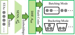
Figure 7: The batching mode and the bucketing model of the DHF, which selects a subset of contending and interfering STAs for the training and the inference of the NGM NN, respectively.

This section explains the DHF in the ScNeuGM that accelerates the NGM by focusing the training and inference of the NGM NN only in those contending and hidden STA pairs. We first explain the design of the DHF in Section V-A and then show the usage of the DHF in the training and the inference of the NGM NN in Sections V-B and V-C, respectively.

V-A Design of Deep Hashing Function

We use a DHF NN with parameters $\theta_{\mathrm{HF}}$ to compute each STA’s hash code based on the STA’s state embeddings as

$$\mathbf{b}_{k}\triangleq[b_{k}^{1},\dots,b_{k}^{\Lambda}]=\mathrm{DHF}(\mathbf{v}_{k}|\theta_{\mathrm{HF}}),\ \forall k,$$ (25)

where $b_{k}^{n}\in\{-1,1\}$ for $n=1,\dots,\Lambda$, and $\Lambda$ is the number of bits in each hash code. To train the DHF, part of the loss is designed to adjust the similarity between codes based on the contention and interference indicators $O^{\mathrm{C}}_{i,j}+O^{\mathrm{H}}_{i,j}$ as

$$L^{\prime}(\theta_{\mathrm{HF}})=\frac{1}{|\mathcal{E}|}\sum_{i\neq j}\big{[}\frac{1}{2\Lambda}(\sum_{n=1}^{\Lambda}b_{i}^{n}b_{j}^{n}+\Lambda)-(O^{\mathrm{C}}_{i,j}+O^{\mathrm{H}}_{i,j})\big{]}^{2},$$ (26)

where $\frac{1}{2\Lambda}(\sum_{n=1}^{\Lambda}b_{i}^{n}b_{j}^{n}+\Lambda)$ is the normalized Hamming distance between STAs $i$ and $j$’s hash codes. The loss in (26) reduces the Hamming distances between STAs’ codes if they are contending or hidden from each other, or otherwise increases the Hamming distances. Further, to ensure that each bit encodes different information about the STAs’ states, part of the loss is designed to reduce the correlation between bit positions in the hash codes as [39]

$$L^{\prime\prime}(\theta_{\mathrm{HF}})=\frac{1}{K^{2}}\|[\mathbf{b}_{1},\dots,\mathbf{b}_{K}][\mathbf{b}_{1},\dots,\mathbf{b}_{K}]^{\rm T}-\mathbb{I}^{K\times K}\|_{2}^{2},$$ (27)

where $[\mathbf{b}_{1},\dots,\mathbf{b}_{K}][\mathbf{b}_{1},\dots,\mathbf{b}_{K}]^{\rm T}$ is the matrix with off-diagonal elements that measure the correlations between bit positions. The total loss of the DHF is

$$L(\theta_{\mathrm{HF}})=L^{\prime}(\theta_{\mathrm{HF}})+\lambda L^{\prime\prime}(\theta_{\mathrm{HF}}).$$ (28)

where $\lambda>0$ is the weight of the correlation loss part in the total loss. The training of the DHF is outlined in Algorithm 1. The applications of the DHF are explained below.

Algorithm 1 Training of the DHF

1: Set training steps $M$ and the learning rate $\eta$.

2: Randomly initialize the DHF parameters, $\theta_{\mathrm{HF}}$.

3: for step $1,\dots,M$ do

4:  Randomly generate a network with $K$ STAs.

5:  Embed STA states using the trained SENN as (16).

6:  Compute the hash codes of STA embeddings as (25).

7:  Compute the losses $L(\theta_{\mathrm{HF}})$ as (26)(27)(28).

8:  Update the parameters of the DHF as    $\theta_{\mathrm{HF}}=\theta_{\mathrm{HF}}-\eta\nabla_{\theta_{\mathrm{HF}}}L(\theta_{\mathrm{HF}})$.

9: end for

10: return the trained DHF with $\theta_{\mathrm{HF}}$.

V-B STA Batching Mode of DHF

Based on the hash codes generated by the DHF, we can select a small subset of STAs with a high likelihood of contention and interference for the ES algorithm, reducing the training time.

V-B1 Design of Batching Mode

The batching mode starts by randomly choosing $\Psi$ positions in $n=1,\dots,\Lambda$ without replacement as $n^{\prime}_{1},\dots,n^{\prime}_{\Psi}$. Then, a $\Psi$-bit random binary query code is generated as $q_{1},\dots,q_{\Psi}$. STAs are selected if their hash codes at $n^{\prime}_{1},\dots,n^{\prime}_{\Psi}$ match the random query codes as

$$\mathcal{Q}\leftarrow\mathcal{Q}\cup\{k\in\mathcal{V}|[b_{k}^{n^{\prime}_{1}},\dots,b_{k}^{n^{\prime}_{\Psi}}]=[q_{1},\dots,q_{\Psi}]\},$$ (29)

where $\mathcal{Q}$ represents the selected STAs and is initialized as $\emptyset$. The above process is repeated with a new query code at new random positions in each iteration until $\mathcal{Q}$ contains $K^{\prime}$ STAs. We refer to $\mathcal{Q}$ as the batch of STAs and $K^{\prime}=|\mathcal{Q}|$ as the batch size. Since the DHF is trained to output the same bits in STA hash codes if STAs are contending or hidden, as explained in Section V-A, STAs that are likely contending with and hidden from each other will likely match the query codes and be batched together. This STA batching mode is used when the NGM NN is under training to select a subset of STAs, allowing the training algorithm to focus on those contending and hidden pairs, thereby increasing efficiency.

V-B2 ES with Batching Mode of DHF

To reduce the computing time of the training process of the ES, we design a curriculum learning method [46] using the batching mode of the DHF to gradually increase the number of STAs, i.e., raise the difficulty of the graph modeling task, until it reaches the total number of STAs. Specifically, as shown in Algorithm 2, the ES algorithm starts with a small number of STAs, $K^{\prime}$, and the total number of STAs, $K$. Here, the state embedding, the predictors, and the DHF are pre-trained. The distribution of the edge generator parameters is initialized with the mean $m^{\mu}_{\mathrm{EG}}=0$ and the variance $\exp({\nu^{\mu}_{\mathrm{EG}}})=\sigma^{2}_{\mathrm{0}}$. In each ES iteration, a random Wi-Fi network is simulated, and $K^{\prime}$ STAs are selected using the DHF’s batching mode. After that, the EGNN parameters are sampled from the parameterized distribution, as shown in (22), which constructs the NGM NN with the pre-trained state embedding and predictors, as shown in Fig. 5 of Section IV-A. For the given STA batch, the edges between them are generated using the NGM NN as (16), (18), and (19), forming the graph. Next, the graph is colored, and the slot assignments for the batched STAs are determined accordingly. The assignments are applied in the network, with only the batched STAs transmitting, where the transmission reliabilities are measured, and the reward is computed as in (20). Finally, the EGNN parameters’ distribution is updated in the direction indicated in (24), with $\eta$ as the learning rate. At the end of each iteration, the moving average of the previous rewards is measured as

$$\Omega\leftarrow\gamma\Omega+(1-\gamma)\mathbf{1}_{\{\dot{R}\geq 0\}},$$ (30)

where $\gamma$ is a smoothing factor less than 1. Since the graph’s performance is optimal when $\dot{R}\geq 0$ (or near-optimal, as an approximation of the minimum slots is used in (20)), we use $\mathbf{1}_{\{\dot{R}\geq 0\}}$ as an indicator of whether the NGM NN has satisfactory performance. In (30), if the averaged reward indicator $\Omega$ is greater than $\hat{\Omega}$, i.e., the NGM NN achieves an averaged satisfactory performance with the current number of STAs $K^{\prime}$, then the number of batched STAs $K^{\prime}$ increases by $K^{\prime\prime}$ in the next iteration; otherwise, the algorithm keeps the same number of STAs $K^{\prime}$. The algorithm terminates if it achieves an averaged satisfactory performance with $K$ STAs. The mean of the parameter distribution is returned as the trained EGNN parameters.

Algorithm 2 ES With Batching Mode of the DHF

1: Set the batch size $K^{\prime}$ and the total STA number $K$.

2: Set the learning rate $\eta$ and batch increment step $K^{\prime\prime}$.

3: Train $\theta^{\mu}_{\mathrm{SE}}$, $\theta^{\mu}_{\mathrm{PC}}$ and $\theta^{\mu}_{\mathrm{PH}}$ as the appendix.

4: Train $\theta_{\mathrm{HF}}$ as Algorithm 1.

5: Initialize $m^{\mu}_{\mathrm{EG}}=0$ and $\exp({\nu^{\mu}_{\mathrm{EG}}})=\sigma^{2}_{\mathrm{0}}$.

6: for step $1,2,\dots$ do

7:  Set up a Wi-Fi network with $K$ STAs.

8:  Select $K^{\prime}$ STAs using the batching mode of the DHF.

9:  Sample the EGNN parameters $\tilde{\theta}^{\mu}_{\mathrm{EG}}$ as (22).

10:  Generate edges in the batch as (16), (18) and (19).

11:  Color the graph using greedy coloring, $\mathbf{z},Z=\chi(\mathbf{E})$.

12:  Apply the slot assignments as $\mathbf{z}$ and $Z$.

13:  Measure reliabilities and obtain the reward $\dot{R}$ as (20).

14:  Estimate update directions of $m^{\mu}_{\mathrm{EG}}$ and $\nu^{\mu}_{\mathrm{EG}}$ in (24).

15:  Update $m^{\mu}_{\mathrm{EG}}$ and $\nu^{\mu}_{\mathrm{EG}}$ as  $m^{\mu}_{\mathrm{EG}}\leftarrow m^{\mu}_{\mathrm{EG}}-\eta\nabla_{m^{\mu}_{\mathrm{EG}}}L(\theta^{\mu}_{\mathrm{EG}})$;   $\nu^{\mu}_{\mathrm{EG}}\leftarrow\nu^{\mu}_{\mathrm{EG}}-\eta\nabla_{\nu^{\mu}_{\mathrm{EG}}}L(\theta^{\mu}_{\mathrm{EG}})$.

16:  Evaluate the reward performance indicator $\Omega$ as (30).

17:  if $\Omega\geq\hat{\Omega}$ then

18:   if $K^{\prime\prime}=K$ then break.

19:   else $K^{\prime}\leftarrow\min\{K^{\prime}+K^{\prime\prime},K\}$.

20:  end if

21: end for

22: return the trained EGNN with $\theta^{\mu}_{\mathrm{EG}}=m^{\mu}_{\mathrm{EG}}$.

V-C STA Bucketing Mode of DHF

Furthermore, we use the DHF to bucket those highly likely contending and hidden STA pairs and generate edges only between them to reduce the computing time of the inference of the trained NGM NN.

V-C1 Design of Bucketing Mode

The bucketing mode randomly chooses $\Psi$ positions in $n=1,\dots,\Lambda$ without replacement as $n^{\prime}_{1},\dots,n^{\prime}_{\Psi}$. A hash table is constructed based on STAs’ hash codes at the chosen positions. Let $\mathcal{C}$ be the set of all hash codes at the selected positions in the table as

$$\mathcal{C}\leftarrow\cup_{k}\{[b_{k}^{n^{\prime}_{1}},\dots,b_{k}^{n^{\prime}_{\Psi}}]\}.$$ (31)

Then, for every code in $\mathcal{C}$, a bucket of STAs is collected if they have the same codes in the selected positions as

$$\mathcal{B}(\mathbf{q})\leftarrow\{k\in\mathcal{V}|[b_{k}^{n^{\prime}_{1}},\dots,b_{k}^{n^{\prime}_{\Psi}}]=\mathbf{q}\},\ \forall\mathbf{q}\in\mathcal{C},$$ (32)

The above process in (31) and (32) is repeated to construct $\Upsilon$ hash tables, bucketing a sufficient number of STA pairs for edge generation as

$$\mathcal{P}\leftarrow\mathcal{P}\cup\left(\cup_{\mathbf{q}\in\mathcal{C}}\{(i,j)|i\in\mathcal{B}(\mathbf{q})\land j\in\mathcal{B}(\mathbf{q}),i\neq j\}\right),$$ (33)

where new random $\Psi$ positions are chosen in each repetition. Here, $\mathcal{P}$ represents the STA pairs requiring NGM NN operations and is initialized as $\emptyset$. The edges between STAs in the same bucket are generated using the NGM NN, as described in Section IV-A, while the edge values for those non-bucketed pairs are ignored and are set to $0$, as

$$E_{i,j}\leftarrow\mu(\mathcal{S}_{i},\mathcal{S}_{j}|\theta^{\mu}),\forall(i,j)\in\mathcal{P};\ E_{i,j}\leftarrow 0,\forall(i,j)\notin\mathcal{P}.$$ (34)

Since the hash codes of contending and hidden STAs are close, they are more likely to be grouped in the same bucket, and edges between them are processed, while edges between less likely contending or hidden STAs are ignored. This STA bucketing mode is used when the trained NGM NN is deployed online across the entire network to reduce the processed edges, i.e., to reduce the complexity of the inference of the NGM NN.

V-C2 Online Graph Modeling with Bucketing Model of DHF

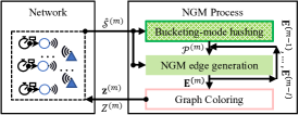
Figure 8: Illustration of the online graph modeling architecture.

We then present the online graph modeling architecture that deploys the NGM NN with the bucketing model of the DHF, as shown in Fig. 8. Note that we assume the NGM NN has been trained and its parameter is not updated further. In this architecture, the NGM process outputs the graph and slot assignments according to online-measured network states and runs in parallel with the network.

In the $m$-th round of the NGM process, $m=1,2,\dots$, the network measures the states $\hat{\mathcal{S}}^{(m)}$, e.g., based on the previous transmissions. Then, the NGM process uses the bucketing mode of the DHF to identify the STA pairs likely contending or interfering, indicated in $\mathcal{P}^{(m)}$, as shown in (33). Since the bucketing mode may miss some STA pairs, the process combines $\mathcal{P}^{(m)}$ with STA pairs that had edges generated in the previous $I$ rounds as

$$\mathcal{P}^{(m)}\leftarrow\mathcal{P}^{(m)}\cup\big{(}\cup_{m^{\prime}=1,\dots,I}\{(i,j)|E_{i,j}^{(m-m^{\prime})}=1\}\big{)}.$$ (35)

This is because previously generated edges are more likely to be generated in the following rounds. Here, $E_{i,j}^{(m-m^{\prime})}$ in (35) represents the edge value between STAs $i$ and $j$ in the $(m-m^{\prime})$-th round. The NGM then generates the edges between each of these pairs, forming the graph with the adjacency matrix $\mathbf{E}^{(m)}$. The slot assignments, $\mathbf{z}^{(m)}$ and $Z^{(m)}$, are determined by coloring this graph. The process takes a duration of $\tau^{(m)}$ milliseconds for the NGM process to perform the bucketing hashing, the graph modeling, and the slot assignments in total. Note that the network makes no transmissions during the first round of the NGM process, i.e., during the first $\tau^{(1)}$ milliseconds. After the slot assignments are returned from the NGM process to the network, the network starts STA transmissions with the assignments, and the NGM process begins the next round of assignments. The above process repeats until the network stops.

VI Simulation Results

This section evaluates our proposed methods in simulations.

VI-A Simulation Configurations

We use NS-3 [40] to simulate Wi-Fi networks with the RTWT mechanism. All devices are located in a 100m$\times$100m squared area centered at the coordinates $(50,50)$ meters, simulating a factory environment [47]. We assume the network has $A=100$ APs, and they are located at the grid in the simulated area, i.e., they are at the coordinates $(5+10x,5+10y)$ meters, where $(x,y)$ are the indices of APs in $x$ and $y$ axes, i.e., $x=1,\dots,10$ and $y=1,\dots,10$. Unless specified otherwise, STAs are static, and the total number of STAs is $K=1000$. Each STA is randomly distributed within the simulated area, with each coordinate selected randomly from a uniform distribution within the interval $[0,100]$ meters. The duration of a RTWT slot is $\Delta_{\mathrm{0}}=500$ microseconds. The channel bandwidth is $B=20$ MHz at a 5.8-GHz carrier frequency. The transmission power of STAs is $\mathbf{P}_{\mathrm{0}}=0$ dBm, and the noise power is set as $\mathbb{N}_{\mathrm{0}}B=-96$ dBm. The path losses between any two devices (including all APs and STAs) follow a log-distance path loss model [48] as $-28\log_{10}(l+1)-20\log_{10}(f/(1\text{MHz}))+12$ in decibel scale, where $f$ is the carrier frequency in MHz and $l$ is the distance between two devices in meters. The receiver sensitivity threshold is set (in decibel scale) to $\mathbf{P}_{\mathrm{0}}-s_{\max}=-95$ dBm. The packet size $L$ is 800 bits. The actual decoding error probability of each transmission is computed using the same equation in (2), where $\phi$ is the signal-to-interference-plus-noise of each transmission instead. This is implemented as a transmission error model in NS-3. The target reliability of each STA is $\hat{r}=0.99$.

The dimensions of the embedding vectors $\mathbf{v}_{k}$ $\forall k$ and the hash codes $\mathbf{b}_{k}$ $\forall k$ are $5$ and $30$, respectively. The configurations of all FNNs are listed in Table I, including the size of each layer, the hidden layer activation functions (HAFs), and the output activation functions (OAFs). Here, the FNNs at the input and output of the SENN are denoted as SENNI and SENNO, respectively. The number of LSTM layers in the state embedding and the decoder is $\xi=2$. The weight of the correlation loss in the DHF’s total loss is $\lambda=0.2$. The learning rate is $\eta=10^{-3}$ for training the state embedding, the predictors, and the DHF, and the corresponding training steps $M$ are $2000$, $2000$, and $10000$, respectively. For training of the EGNN using the ES, the smoothing factor in (30) is $\gamma=0.9$; the threshold for the reward performance to increase STAs is $\hat{\Omega}=0.9$; the number of STAs added in each increment is $K^{\prime\prime}=50$; the learning rate is $\eta=10^{-1}$. The initial variance of the EGNN parameters is $\sigma^{2}_{\mathrm{0}}=0.1$. Simulations are conducted on a MacBook with the M4 chip.

TABLE I: Configurations of All FNNs

NNs	Dimensions of layers	HAFs	OAFs
SENNI	$3,15,15,15$	$\mathrm{GELU}(\cdot)$	$\mathrm{GELU}(\cdot)$
SENNO	$15,5$	None	None
PCNN	$10,50,50,1$	$\mathrm{ReLU}(\cdot)$	$\mathrm{Sigmoid}(\cdot)$
PHNN	$10,50,50,1$	$\mathrm{ReLU}(\cdot)$	$\mathrm{Sigmoid}(\cdot)$
DHF	$5,30,30,30,30,30$	$\mathrm{GELU}(\cdot)$	$\mathrm{Tanh}(\cdot)$
EGNN	$5,50,50,1$	$\mathrm{ReLU}(\cdot)$	$\mathrm{Sigmoid}(\cdot)$

VI-B Baseline Methods

We explain the baseline methods, other than the proposed methods. Note that since contention and interference are not measured from the network, the Markov models can hardly estimate the STA QoS. Additionally, the GNN models can hardly provide useful slot assignment decisions in graph-coloring-structured problems based on previous observations in [35] and justifications in [26, 27]. Thus, we compare the remaining approaches reviewed in Section I-A, including heuristic graph models and the NGM with PG or DPG. Their detailed implementations are explained as follows.

VI-B1 Heuristic Graph Models (IFG, CHG)

We compare the heuristic graph models used to construct binary graphs with manually designed rules. The work in [21] connects two STAs if the same AP can detect them, i.e., $E_{i,j}=\mathbf{1}_{\{\mathcal{A}_{i}\cap\mathcal{A}_{j}\neq\emptyset\}}$ for all $i\neq j$, referred to as the “IFG” scheme. Since STAs’ transmissions are primarily affected by contention and interference in the network, we also compare the graph constructed using the contention and interference indicators, where $E_{i,j}=O^{\mathrm{C}}_{i,j}+O^{\mathrm{H}}_{i,j}$ for all $i\neq j$, referred to as the “CHG” scheme. Note that the CHG scheme is only applied for comparison and is impractical in real-world networks due to the unmeasured contention and interference indicators.

VI-B2 NGM Requiring Edge-Wise Feedback (PG, DPG)

We compare the designed ES algorithm with the PG [34] and DPG [36] algorithms when training the NGM NN. Specifically, the PG algorithm uses the log-derivative trick to estimate the gradient of the performance w.r.t. each edge value in (15) as

$$\frac{\partial L(\theta^{\mu})}{\partial E_{i,j}}=\frac{(\dot{R}-\bar{R})\partial\log E_{i,j}}{\partial E_{i,j}},\ \forall i\neq j,$$ (36)

where $E_{i,j}\in[0,1]$ is interpreted as the probability that an edge exists between STA $i$ and STA $j$. For the DPG, the gradient w.r.t. the edges are estimated based on the back-propagation on another NN that approximates the performance given edge values and STA states as

$$\frac{\partial L(\theta^{\mu})}{\partial E_{i,j}}=\frac{\partial Q(\mathbf{E},\hat{\mathcal{S}}|\theta^{Q})}{\partial E_{i,j}},\ \forall i\neq j,$$ (37)

where $Q(\cdot|\theta^{Q})$, referred to as the critic, is trained to minimize the difference between its output and the reward [35].

VI-C Training Convergence of SENN, PCNN, PHNN and DHF

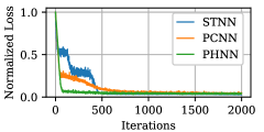
(a) Pre-training of the NGM NN components.

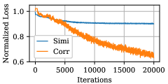
(b) Training of the DHF.

Figure 9: Normalized loss values during training processes of the SENN, the PCNN, the PHNN and the DHF.

We first show the loss values in the training process of the SENN, the PCNN and the PHNN in Fig. 9a, where the loss values are normalized against their initial values during training. Results show that the loss values decrease over the training steps and converge in less than 500 steps when training the NGM NN components, the state embedding and the predictors. Fig. 9b shows that the DHF’s losses, i.e., the similarity loss (with legend “Simi”) and the correlation loss (with legend “Corr”), converge over the iteration in Algorithm 1. Results imply that the NNs, including the state embedding, the predictors, and the DHF, are well-trained and used in the following simulations without further updates to their parameters.

VI-D Configurations of Batching/Bucketing Modes of DHF

Based on the trained DHF, we then test the batching and bucketing modes. First, for the batching mode, we run the ES algorithm with a fixed small number of STAs, $K^{\prime}=20$, selected (i.e., without curriculum learning). The reward performance is measured as the moving average of the indicator $\mathbf{1}_{\dot{R}\geq 0}$ at each step. Fig. 10a compares the performance of the batching mode when using different numbers of query bits, from $\Psi=0$ to $10$, where $\Psi=0$ means the STAs are chosen randomly without using the DHF. The results indicate that the ES algorithm struggles to converge when using fewer query bits, e.g., $\Psi=0,1,2$. This is because the selected STAs are independent of their contention and interference, and they are likely to have no contention or interference between them. As a result, the NGM NN finds it difficult to learn to separate contending or hidden STAs. The convergence improves when $\Psi=3,4$. This is because more query bits lead to a higher proportion of contending or interfering STA pairs in the selected batch, which enhances training efficiency. However, the convergence slows slightly when $\Psi>4$ because the batch becomes highly biased toward contending or hidden STA pairs, and the NGM NN struggles to learn when not to separate STA pairs within the batch. Second, for the bucketing mode, we measure the proportion of hashed STA pairs from all possible STA pairs (with legend “Pair Count”), and the proportion of hashed contending or hidden pairs from all contending or hidden pairs (with legend “Recall”). Fig. 10b compares the above metrics for different numbers of query bits, from $\Psi=1$ to $15$, and hash tables, from $\Upsilon=1$ to $30$. The results show that with fewer query bits and more hash tables, more STA pairs are hashed, and the recall rate is higher. Since we aim to reduce the number of hashed STA pairs while increasing the number of hashed contending or hidden pairs among all hashed pairs, we subtract “Pair Count” from “Recall” to measure the efficiency of the bucketing mode (with legend “Efficiency”). The results indicate that $\Psi\approx 7$ and $\Upsilon\geq 20$ achieve the best efficiency. In summary, we fix $\Psi=4$ in the batching mode and $\Psi=7$ and $\Upsilon=20$ in the bucketing mode in the rest of the simulations.

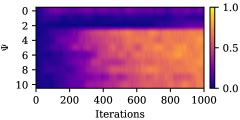
(a) The reward of the batching mode with different numbers of query bits, $\Psi$, when $K^{\prime}=20$.

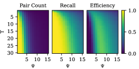
(b) The performance of the bucketing mode with different numbers of query bits, $\Psi$, and hash tables, $\Upsilon$.

Figure 10: The performance of the trained DHF.

VI-E Performance of ES with Batching Mode of DHF

Next, we illustrate the ES algorithm’s performance.

VI-E1 Comparison with PG and DPG

We compare the performance of the ES with the PG and the DPG when a fixed small number of STAs is selected using the batching mode of the DHF, i.e., $K^{\prime}=20$. The performance is measured based on the QoS violations, the ratio of approximated optimal slots to the number of used slots, and the averaged reward performance indicator. The results show that the proposed ES algorithm achieves the lowest QoS violation probability, the least number of slots, and the highest reward performance (approximately $4\sim 10$ times higher), while the PG and DPG algorithms struggle to converge to satisfactory performance. This is because the PG and DPG algorithms require STA-pairwise (or edge-wise) gradients, but no STA-pairwise feedback is available. In comparison, the ES algorithm directly applies the reward feedback in the parameter space to improve the NGM NN.

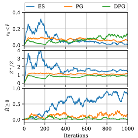
Figure 11: The performance of ES, PG and DPG for the NGM when $K^{\prime}=20$.

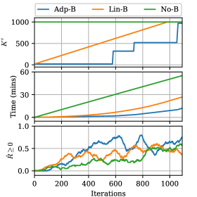
Figure 12: The performance of the ES with different batching schemes.

VI-E2 Performance of ES with Different Batching Schemes

We then show the performance of the ES algorithm with and without the batching mode of the DHF. Specifically, we consider 1) the proposed batching method that adaptively increases the number of STAs, $K^{\prime}$, based on the reward performance (with legend “Adp-B”), as shown in Algorithm 2; 2) a batching method that linearly increases $K^{\prime}$ by one in each step (with the legend “Lin-B”); and 3) a method that uses no batching but trains the NGM NN with the total number of STAs, $K=K^{\prime}$ (with the legend “No-B”). Fig. 12 measures the number of STAs, the training time, and the averaged reward performance indicator during the training steps. The results show that the proposed adaptive batching converges to the target number of STAs at approximately $1100$ steps. Additionally, the performance of all three compared methods is similar around $1100$ steps. However, the training time of the proposed adaptive batching method is approximately $4$ times and $2$ times shorter than that of the linear batching method and the no-batching method, respectively. In other words, the proposed method significantly reduces the training time for the NGM. In the remaining simulations, the trained NGM parameters are fixed as those from the last step of the proposed ES with the adaptive batching, without further updates.

VI-F Performance of NGM with Bucketing Mode of DHF

We evaluate the trained NGM NN online with the bucketing mode of DHF when there are $K=1000$ STAs.

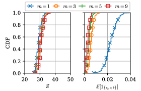
Figure 13: The NGM NN in the architecture when STAs are static.

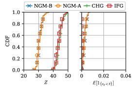
Figure 14: Comparison between the NGM and heuristic graph models.

VI-F1 Performance When STAs are Static

Fig. 13 shows the NGM NN’s performance in the cumulative distribution function (CDF) of the number of used slots and the number of QoS violated STAs when the NGM NN operates for different numbers of rounds, $m$, in the architecture. In this architecture, all STA pairs connected by edges in previous rounds are combined into the processing STA pairs for the current round, as shown in (35). The results show that across different rounds, the number of slots to color the generated graph remains consistent, around $30$ slots. It also shows that the NGM NN in the first round results in $2\%$ of STAs experiencing QoS violations. However, by running the NGM process for more rounds, the QoS violations are fewer than $1\%$. This improvement is due to the bucketing mode in each round, which can miss some contending and interfering STA pairs, as previous simulations in Section VI-D. By adding the previously connected pairs in the NGM process as (35), the likelihood of missing the processing of contending or interfering STA pairs is efficiently reduced.

Fig. 14 compares the number of slots and QoS violations achieved by the NGM with the DHF’s bucketing mode when the number of rounds $m$ is 9 (with legend “NGM-B”), the NGM with all STA pairs processed (with legend “NGM-A”), and the heuristic graph models (with legends “CHG” and “IFG”). The results show that the NGM achieves $25\%$ fewer slots than the heuristic graph models. This is because the NGM allows slot sharing among STA pairs that are not heavily contending or interfering with each other, while the heuristic graph models separate all contending or interfering pairs. Consequently, the heuristic graph models achieve fewer QoS violations but use more slots or cause higher delays in periodicity. The results also show that the scheme with partly processed STA pairs using the DHF’s bucketing mode achieves performance similar to the one where the NGM processes all STA pairs. This implies that only a subset of STA pairs, e.g., those likely to be contending or interfering, requires NGM processing, which further suggests that the DHF’s bucketing mode reduces the complexity when modeling the graph.

VI-F2 Performance When STAs are Mobile

We then show the NGM’s performance when STAs are mobile. Specifically, STAs move in a random direction within the simulated area, with speeds varying from $0$ to $5$ meters per second, approximately the typical walking speeds of mobile robots. Note that when STAs reach the boundary of the simulated area, they move in another random direction toward the inside of the area. We compare the following schemes: 1) the NGM using the DHF’s bucketing mode and combining previous rounds’ edges (the maximum rounds to combine is $I=20$) into the processed pairs (with legend “NGM-B”); 2) the NGM using the DHF’s bucketing mode without combining previous edges in the NGM processed pairs (with legend “No-Comb”); and 3) the NGM processing all edge pairs among STAs (with legend “NGM-A”). Fig. 15 measures the average number of slots and the average packet loss rates in the above schemes. The results show that the average number of slots is similar across all schemes (around $30$ slots), while the NGM-B and NGM-A schemes achieve lower packet loss rates. This is because the NGM-B and NGM-A schemes process more contending or hidden STA pairs than the No-Comb scheme. On the other hand, the NGM-B scheme has $30\%$ fewer packet losses than the NGM-A scheme when STAs have high mobility. This is because the DHF’s bucketing mode selectively processes contending or interfering STA pairs, making the NGM process with the DHF’s bucketing mode faster when modeling the graph. Consequently, it responds more timely to the varying locations of STAs. The detailed computing time of the NGM process is measured next.

VI-G Computational Complexity in Time

We discuss the computational complexity of the proposed methods in terms of the number of STAs, $K$. Training the state embedding (trained over STA-wise), the predictors (trained over STA-pairwise), and the DHF (also trained over STA-pairwise) incurs $\mathcal{O}(K)$, $\mathcal{O}(K^{2})$, and $\mathcal{O}(K^{2})$ complexity, respectively. The batching mode of the DHF requires a $\mathcal{O}(K)$ complexity to compare the random query and collect the batch. Training the EGNN in Algorithm 2 is also processed over STA-pairwise, resulting in an $\mathcal{O}(K^{2})$ complexity. The NGM complexity when modeling/processing the graph depends on the number of STA pairs collected using the bucketing mode of the DHF. Since it is difficult to analyze hash codes/tables generated by DHF, we instead measure the computing time of the NGM process quantitatively. Specifically, Fig. 16 compares the computing time of the NGM process when $K=1000$ in 1) the scheme where the NGM only processes STA pairs collected by the DHF bucketing mode (with legend “NGM-B”), and 2) the scheme where the NGM processes all STA pairs (with legend “NGM-A”). The results show that the DHF’s bucketing mode reduces the computing time for STA-pairwise operations, such as predictors and edge generation, by a factor of $8$, and the total computing time by a factor of $3$. This is because only the STA pairs in the buckets are processed, while the bucketing mode adds some additional computing time when collecting the STA pairs in the buckets/hash tables. Note that the current hash table construction is single-threaded on a central processing unit, while further time reduction can be achieved by an efficient parallelized implementation on a graphics processing unit.

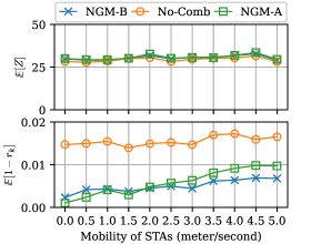
Figure 15: The NGM performance in online architecture when STAs are mobile.

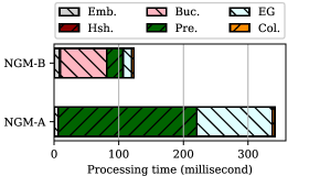
Figure 16: The computing time, $\operatorname{\mathbb{E}}[\tau^{(m)}]$, for the NGM process to model and color the graph, including the time spent by the state embedding (Emb.), the DHF’s hash code generation (Hsh.), the DHF’s bucketing mode (Buc.), the predictors (Pre.), edge/graph generation (EG) and the graph coloring (Col.)

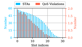
Figure 17: The STA and the QoS Violation counts in different slots.

VI-H Impact of Greedy Graph Coloring

Fig. 17 shows the number of STAs and QoS violations in different slots. The results show that most STAs are assigned to slots with lower indices. This is because the greedy coloring scheme used in this work iteratively assigns STAs to previously added slots (with lower indices), while recently added slots remain almost empty. As a result, more QoS violations occur in the slots with more STAs. An efficient and balanced graph coloring scheme could further improve the QoS [49].

VII Conclusion

This paper presented ScNeuGM for managing contention and interference in Wi-Fi 7 networks through coloring-based slot assignment. ScNeuGM utilized the ES algorithm, which eliminates the reliance on explicit STA-pairwise feedback in the NGM, offering a robust and scalable optimization approach. Furthermore, the ScNeuGM leveraged a DHF to group contending or hidden STAs and reduce the computational complexity of training and inference of the NGM NN. Extensive evaluation demonstrated the scalability and effectiveness of our methods in large Wi-Fi network scenarios. Future work could focus on further optimizing the graph coloring algorithm and accelerating the computation routines in the NGM. Additionally, research could be conducted to explore richer graph representations that integrate the application layer’s context, semantic, and task-oriented information, and to extend the framework to accommodate more heterogeneous network deployments.

Appendix: Proof of Proposition 1

Proof.

To prove this statement, we construct an example that satisfies it. Let $\hat{\mathbf{z}}$ and $\hat{Z}$ be an optimal solution of problem (9). In the adjacency matrix $\hat{\mathbf{E}}$, we set $\hat{E}_{i,j}=1$ for every STA pair $(i,j)$ with different colors and set $\hat{E}_{i,j}=0$ otherwise. In other words, $\hat{\mathbf{E}}$ represents a complete multipartite graph. The graph with $\hat{\mathbf{E}}$ has a unique coloring scheme $\hat{\mathbf{z}}$ and $\hat{Z}$ because any alternative coloring of STAs would cause violations of the edge constraints. Therefore, $\hat{\mathbf{z}},\hat{Z}=\chi(\hat{\mathbf{E}})$, which also solves the contention and interference management problem according to the definition of $\hat{\mathbf{z}}$ and $\hat{Z}$. By providing this example, we demonstrate that an optimal graph exists, thereby proving the statement. ∎

Appendix: Proof of Theorem 1

Proof.

Given the optimal graph $\mathcal{G}^{*}$ with the adjacency matrix $\mathbf{E}^{*}$ and its coloring scheme $\mathbf{z}^{*},Z^{*}=\chi(\mathbf{E}^{*})$, the coloring scheme of the optimal graph, $\mathbf{z}^{*}$ and $Z^{*}$, corresponds to the optimal slot assignment, where all STAs’ reliability constraints are satisfied, and the number of slots is minimized. Suppose we remove all edges between non-contending and non-hidden STAs in $\mathcal{G}^{*}$. This results in a new graph $\mathcal{G}^{\prime}$ with edge values $E^{\prime}_{i,j}=E^{*}_{i,j}\land(O^{\mathrm{C}}_{i,j}+O^{\mathrm{H}}_{i,j})$ for all $i\neq j$. By re-coloring $\mathcal{G}^{\prime}$, STAs in $\mathcal{G}^{\prime}$ will share the same color (or the same slot) if and only if they have no edges between them in $\mathcal{G}^{\prime}$, i.e., they are non-contending and non-hidden STAs, or they were in the same color in $\mathcal{G}^{*}$. In this new color scheme, i.e., $\mathbf{z}^{\prime},Z^{\prime}=\chi(\mathbf{E}^{\prime})$, each STA now shares the slot only with: 1) STAs that are neither contending with nor hidden from it, or 2) those STAs that were sharing slots in the previous optimal graph $\mathcal{G}^{*}$. Note that each STA’s transmissions are not affected by non-contending and non-hidden STAs, and the slot-sharing STAs in the previous graph $\mathcal{G}^{*}$ have reliable transmissions, according to the definition of its optimality. Therefore, the coloring scheme of the new graph $\mathcal{G}^{\prime}$, i.e., $\mathbf{z}^{\prime}$ and $Z^{\prime}$, ensures reliable transmissions, thus satisfying the constraints. Note that $\mathcal{G}^{\prime}$ is generated by edge removal from $\mathcal{G}^{*}$. Thus, their chromatic numbers satisfy $Z^{\prime}\leq Z^{*}$. Further, according to the optimality of $\mathcal{G}^{*}$, $Z^{*}$ is the minimum number of slots required to ensure reliability, implying that $Z^{\prime}$ is equal to $Z^{*}$. Therefore, the coloring scheme of $\mathcal{G}^{\prime}$, i.e., $\mathbf{z}^{\prime}$ and $Z^{\prime}$, ensures the reliability constraints and minimizes the number of slots. In other words, $\mathcal{G}^{\prime}$ is optimal, which proves the statement.

Appendix: Pre-training of NGM NN

The SENN is trained as an encoder NN that maps the STA state sequence into an embedding vector, along with a decoder NN to recover the sequence from the embedding vector. The decoder $\mathrm{DCNN}(\cdot|\theta^{\mu}_{\mathrm{DC}})$ has the same structure as the encoder but uses different parameters, $\theta^{\mu}_{\mathrm{DC}}$, and recovers the sequence from $\mathbf{v}_{k}$ as

$$\tilde{\mathcal{S}}_{k}\triangleq\{\tilde{\mathbf{s}}_{k}(1),\dots,\tilde{\mathbf{s}}_{k}(|\mathcal{A}_{k}|)\}=\mathrm{DCNN}(\mathbf{v}_{k}|\theta_{\mathrm{DC}}),\ \forall k,$$ (38)

where $\tilde{\mathcal{S}}_{k}$ is the recovered sequence. In the decoder, each LSTM block in the first layer takes $\mathbf{v}_{k}$ as input, and the recovered sequence is obtained as the collection of output gate vectors from the LSTM blocks in the last layer. The loss function of the SENN is designed to minimize the difference between the original and recovered state sequences using the mean squared error as

$$L(\theta^{\mu}_{\mathrm{SE}},\theta_{\mathrm{DC}})=\frac{1}{K}\sum_{k=1}^{K}\sum_{a=1}^{|\mathcal{A}_{k}|}\|\mathbf{s}_{k}(a)-\tilde{\mathbf{s}}_{k}(a)\|_{2}^{2}.$$ (39)

The SENN (the encoder NN) and the decoder NN are updated over the above loss functions using stochastic gradient descent with a learning rate $\eta$ for $M$ iterations. Note that only the SENN (the encoder) is used in the NGM NN to embed the state sequences, as shown in Fig. 5, while the decoder is not a component of the NGM NN.

The loss functions of the predictors are designed to minimize the difference between the true values and the predicted ones using binary cross-entropy as

$$L(\theta^{\mu}_{\mathrm{PC}}) =\sum_{i\neq j}O^{\mathrm{C}}_{i,j}\log_{2}\tilde{O}^{\mathrm{C}}_{i,j}+(1-O^{\mathrm{C}}_{i,j})\log_{2}(1-\tilde{O}^{\mathrm{C}}_{i,j});$$ (40)

$$L(\theta^{\mu}_{\mathrm{PH}}) =\sum_{i\neq j}O^{\mathrm{H}}_{i,j}\log_{2}\tilde{O}^{\mathrm{H}}_{i,j}+(1-O^{\mathrm{H}}_{i,j})\log_{2}(1-\tilde{O}^{\mathrm{H}}_{i,j}).$$

The predictors are updated using stochastic gradient descent over the above loss functions with a learning rate $\eta$ for $M$ iterations. Note that both predictor parameters, $\theta^{\mu}_{\mathrm{PC}}$ and $\theta^{\mu}_{\mathrm{PH}}$, are components of the NGM NN, as illustrated in Fig. 5.

∎

References

- [1] C. Deng, X. Fang, X. Han, X. Wang, L. Yan, R. He, Y. Long, and Y. Guo, “IEEE 802.11be Wi-Fi 7: New Challenges and Opportunities,” IEEE Communications Surveys & Tutorials, vol. 22, no. 4, pp. 2136–2166, 2020.
- [2] A. Garcia-Rodriguez, D. López-Pérez, L. Galati-Giordano, and G. Geraci, “IEEE 802.11be: Wi-Fi 7 Strikes Back,” IEEE Communications Magazine, vol. 59, no. 4, pp. 102–108, Apr. 2021.
- [3] L. Galati-Giordano, G. Geraci, M. Carrascosa, and B. Bellalta, “What will Wi-Fi 8 be? A primer on IEEE 802.11 bn ultra high reliability,” IEEE Communications Magazine, vol. 62, no. 8, pp. 126–132, 2024.
- [4] A. Nasrallah, A. S. Thyagaturu, Z. Alharbi, C. Wang, X. Shao, M. Reisslein, and H. ElBakoury, “Ultra-low latency (ULL) networks: The IEEE TSN and IETF DetNet standards and related 5G ULL research,” IEEE Communications Surveys & Tutorials, vol. 21, no. 1, pp. 88–145, 2018.
- [5] D. Cavalcanti, C. Cordeiro, M. Smith, and A. Regev, “WiFi TSN: Enabling Deterministic Wireless Connectivity over 802.11,” IEEE Communications Standards Magazine, vol. 6, no. 4, pp. 22–29, Dec. 2022.
- [6] K. Zanbouri, Md. Noor-A-Rahim, J. John, C. J. Sreenan, H. V. Poor, and D. Pesch, “A Comprehensive Survey of Wireless Time-Sensitive Networking (TSN): Architecture, Technologies, Applications, and Open Issues,” IEEE Communications Surveys & Tutorials, pp. 1–1, 2024.
- [7] A. Karamyshev, M. Liubogoshchev, A. Lyakhov, and E. Khorov, “Enabling Industrial Internet of Things With Wi-Fi 6: An Automated Factory Case Study,” IEEE Transactions on Industrial Informatics, pp. 1–11, 2024.
- [8] 3GPP, “Service requirements for cyber-physical control applications in vertical domains,” 3GPP, TS 22.104, 2018.
- [9] IEEE, “IEEE Standard for Information Technology–Telecommunications and Information Exchange between Systems - Local and Metropolitan Area Networks–Specific Requirements - Part 11: Wireless LAN Medium Access Control (MAC) and Physical Layer (PHY) Specifications,” IEEE Std 802.11-2020 (Revision of IEEE Std 802.11-2016), pp. 1–4379, Feb. 2021.
- [10] G. Bianchi, “Performance analysis of the IEEE 802.11 distributed coordination function,” IEEE Journal on Selected Areas in Communications, vol. 18, no. 3, pp. 535–547, Mar. 2000.
- [11] M. Garetto, T. Salonidis, and E. Knightly, “Modeling Per-Flow Throughput and Capturing Starvation in CSMA Multi-Hop Wireless Networks,” IEEE/ACM Transactions on Networking, vol. 16, no. 4, pp. 864–877, Aug. 2008.
- [12] M. Nurchis and B. Bellalta, “Target Wake Time: Scheduled Access in IEEE 802.11ax WLANs,” IEEE Wireless Communications, vol. 26, no. 2, pp. 142–150, Apr. 2019.
- [13] C. Yang, J. Lee, and S. Bahk, “Target Wake Time Scheduling Strategies for Uplink Transmission in IEEE 802.11ax Networks,” in 2021 IEEE Wireless Communications and Networking Conference (WCNC). Nanjing, China: IEEE, Mar. 2021, pp. 1–6.
- [14] J. Haxhibeqiri, X. Jiao, X. Shen, C. Pan, X. Jiang, J. Hoebeke, and I. Moerman, “Coordinated SR and Restricted TWT for Time Sensitive Applications in WiFi 7 Networks,” IEEE Communications Magazine, vol. 62, no. 8, pp. 118–124, Aug. 2024.
- [15] E. Khorov, A. Kiryanov, A. Lyakhov, and G. Bianchi, “A Tutorial on IEEE 802.11ax High Efficiency WLANs,” IEEE Communications Surveys & Tutorials, vol. 21, no. 1, pp. 197–216, 2019.
- [16] T.-C. Chang, C.-H. Lin, K. C.-J. Lin, and W.-T. Chen, “Traffic-aware sensor grouping for IEEE 802.11 ah networks: Regression based analysis and design,” IEEE Transactions on Mobile Computing, vol. 18, no. 3, pp. 674–687, 2018.
- [17] C. Kai, J. Zhang, X. Zhang, and W. Huang, “Energy-efficient sensor grouping for IEEE 802.11 ah networks with max-min fairness guarantees,” IEEE Access, vol. 7, pp. 102 284–102 294, 2019.
- [18] B. Nardelli and E. W. Knightly, “Closed-form throughput expressions for CSMA networks with collisions and hidden terminals,” in 2012 Proceedings IEEE INFOCOM. Orlando, FL, USA: IEEE, Mar. 2012, pp. 2309–2317.
- [19] A. Subramanian, H. Gupta, S. Das, and Jing Cao, “Minimum Interference Channel Assignment in Multiradio Wireless Mesh Networks,” IEEE Transactions on Mobile Computing, vol. 7, no. 12, pp. 1459–1473, Dec. 2008.
- [20] A. Mishra, S. Banerjee, and W. Arbaugh, “Weighted coloring based channel assignment for WLANs,” ACM SIGMOBILE Mobile Computing and Communications Review, vol. 9, no. 3, pp. 19–31, Jul. 2005.
- [21] Q. Chen, “An energy efficient channel access with target wake time scheduling for overlapping 802.11 ax basic service sets,” IEEE Internet of Things Journal, 2022.
- [22] S. Szott, K. Kosek-Szott, P. Gawłowicz, J. T. Gómez, B. Bellalta, A. Zubow, and F. Dressler, “Wi-Fi meets ML: A survey on improving IEEE 802.11 performance with machine learning,” IEEE Communications Surveys & Tutorials, vol. 24, no. 3, pp. 1843–1893, 2022.
- [23] Z. Gu, C. She, W. Hardjawana, S. Lumb, D. McKechnie, T. Essery, and B. Vucetic, “Knowledge-assisted deep reinforcement learning in 5G scheduler design: From theoretical framework to implementation,” IEEE Journal on Selected Areas in Communications, vol. 39, no. 7, pp. 2014–2028, 2021.
- [24] Y. Shen, Y. Shi, J. Zhang, and K. B. Letaief, “Graph neural networks for scalable radio resource management: Architecture design and theoretical analysis,” IEEE Journal on Selected Areas in Communications, vol. 39, no. 1, pp. 101–115, 2020.
- [25] M. Eisen and A. Ribeiro, “Optimal wireless resource allocation with random edge graph neural networks,” IEEE Transactions on Signal Processing, vol. 68, pp. 2977–2991, 2020.
- [26] K. Xu, W. Hu, J. Leskovec, and S. Jegelka, “How Powerful are Graph Neural Networks?” in International Conference on Learning Representations, Sep. 2018.
- [27] A. Loukas, “What graph neural networks cannot learn: Depth vs width,” in International Conference on Learning Representations, Sep. 2019.
- [28] H. Lemos, M. Prates, P. Avelar, and L. Lamb, “Graph colouring meets deep learning: Effective graph neural network models for combinatorial problems,” in 2019 IEEE 31st International Conference on Tools with Artificial Intelligence (ICTAI). IEEE, 2019, pp. 879–885.
- [29] M. J. A. Schuetz, J. K. Brubaker, Z. Zhu, and H. G. Katzgraber, “Graph coloring with physics-inspired graph neural networks,” Physical Review Research, vol. 4, no. 4, p. 043131, Nov. 2022.
- [30] X. Guo and L. Zhao, “A Systematic Survey on Deep Generative Models for Graph Generation,” IEEE Transactions on Pattern Analysis and Machine Intelligence, vol. 45, no. 5, pp. 5370–5390, May 2023.
- [31] X. Chen, Y. Wang, J. He, Y. Du, S. Hassoun, X. Xu, and L.-P. Liu, “Graph Generative Pre-trained Transformer,” arXiv e-prints, no. arXiv:2501.01073, Jan. 2025.
- [32] J. Wang, Y. Liu, H. Du, D. Niyato, J. Kang, H. Zhou, and D. I. Kim, “Empowering Wireless Networks with Artificial Intelligence Generated Graph,” arXiv e-prints, no. arXiv:2405.04907, May 2024.
- [33] C. Zhao, G. Liu, B. Xiang, D. Niyato, B. Delinchant, H. Du, and D. I. Kim, “Generative AI Enabled Robust Sensor Placement in Cyber-Physical Power Systems: A Graph Diffusion Approach,” arXiv e-prints, no. arXiv:2501.06756, Jan. 2025.
- [34] R. S. Sutton, D. McAllester, S. Singh, and Y. Mansour, “Policy Gradient Methods for Reinforcement Learning with Function Approximation,” in Advances in Neural Information Processing Systems, vol. 12. MIT Press, 1999.
- [35] Z. Gu, B. Vucetic, K. Chikkam, P. Aliberti, and W. Hardjawana, “Graph Representation Learning for Contention and Interference Management in Wireless Networks,” IEEE/ACM Transactions on Networking, vol. 32, no. 3, pp. 2479–2494, Jun. 2024.
- [36] T. P. Lillicrap, J. J. Hunt, A. Pritzel, N. Heess, T. Erez, Y. Tassa, D. Silver, and D. Wierstra, “Continuous control with deep reinforcement learning,” arXiv e-prints, no. arXiv:1509.02971, Jul. 2019.
- [37] D. Wierstra, T. Schaul, T. Glasmachers, Y. Sun, J. Peters, and J. Schmidhuber, “Natural evolution strategies,” The Journal of Machine Learning Research, vol. 15, no. 1, pp. 949–980, 2014.
- [38] T. Salimans, J. Ho, X. Chen, S. Sidor, and I. Sutskever, “Evolution Strategies as a Scalable Alternative to Reinforcement Learning,” arXiv e-prints, no. arXiv:1703.03864, Sep. 2017.
- [39] X. Luo, H. Wang, D. Wu, C. Chen, M. Deng, J. Huang, and X.-S. Hua, “A Survey on Deep Hashing Methods,” ACM Transactions on Knowledge Discovery from Data, vol. 17, no. 1, pp. 1–50, Feb. 2023.
- [40] NS-3, “Network Simulator 3,” https://www.nsnam.org/about, 2023.
- [41] W. Yang, G. Durisi, T. Koch, and Y. Polyanskiy, “Quasi-static multiple-antenna fading channels at finite blocklength,” IEEE Transactions on Information Theory, vol. 60, no. 7, pp. 4232–4265, 2014.
- [42] D. B. West et al., Introduction to graph theory. Prentice hall Upper Saddle River, 2001, vol. 2.
- [43] G. E. Hinton and R. R. Salakhutdinov, “Reducing the Dimensionality of Data with Neural Networks,” Science, vol. 313, no. 5786, pp. 504–507, Jul. 2006.
- [44] I. Sutskever, O. Vinyals, and Q. V. Le, “Sequence to Sequence Learning with Neural Networks,” in Advances in Neural Information Processing Systems, vol. 27. Curran Associates, Inc., 2014.
- [45] V. Mnih, A. P. Badia, M. Mirza, A. Graves, T. Lillicrap, T. Harley, D. Silver, and K. Kavukcuoglu, “Asynchronous Methods for Deep Reinforcement Learning,” in Proceedings of The 33rd International Conference on Machine Learning. PMLR, Jun. 2016, pp. 1928–1937.
- [46] X. Wang, Y. Chen, and W. Zhu, “A Survey on Curriculum Learning,” IEEE Transactions on Pattern Analysis and Machine Intelligence, vol. 44, no. 9, pp. 4555–4576, Sep. 2022.
- [47] 3GPP, “Study on NR industrial internet of things (IoT),” 3GPP, TS 38.825, 2019.
- [48] P. Series, “Propagation data and prediction methods for the planning of indoor radiocommunication systems and radio local area networks in the frequency range 300 MHz to 100 GHz,” Recommendation ITU-R, pp. 1238–8, 2015.
- [49] Z. Gu, J. Park, B. Vucetic, and J. Choi, “SIG-SDP: Sparse Interference Graph-Aided Semidefinite Programming for Large-Scale Wireless Time-Sensitive Networking,” arXiv e-prints, no. arXiv:2501.11307, Jan. 2025.