Efficient sampling approaches based on generalized Golub-Kahan methods for large-scale hierarchical Bayesian inverse problems

Abstract

Uncertainty quantification for large-scale inverse problems remains a challenging task. For linear inverse problems with additive Gaussian noise and Gaussian priors, the posterior is Gaussian but sampling can be challenging, especially for problems with a very large number of unknown parameters (e.g., dynamic inverse problems) and for problems where computation of the square root and inverse of the prior covariance matrix are not feasible. Moreover, for hierarchical problems where several hyperparameters that define the prior and the noise model must be estimated from the data, the posterior distribution may no longer be Gaussian, even if the forward operator is linear. Performing large-scale uncertainty quantification for these hierarchical settings requires new computational techniques. In this work, we consider a hierarchical Bayesian framework where both the noise and prior variance are modeled as hyperparameters. Our approach uses Metropolis-Hastings independence sampling within Gibbs where the proposal distribution is based on generalized Golub-Kahan based methods. We consider two proposal samplers, one that uses a low rank approximation to the conditional covariance matrix and another that uses a preconditioned Lanczos method. Numerical examples from seismic imaging, dynamic photoacoustic tomography, and atmospheric inverse modeling demonstrate the effectiveness of the described approaches.

MSC Classification]65F22, 65M32, 62F10

1 Introduction

Inverse problems arise in many scientific applications, where the main goal is to use collected measurements or observations to estimate some underlying unknown parameters of physical models. We focus on inverse problems in imaging, where the unknown parameters represent detailed spatial or spatiotemporal reconstructions of physical properties such as images of attenuation coefficients in X-ray tomography or spatiotemporal maps of greenhouse gas emission fluxes in atmospheric inverse modeling [1]. For example, in dynamic inverse problems, the unknown parameters can change over time, easily resulting in millions of unknown parameters. For example, in dynamic atmospheric inverse modeling, the goal is to estimate thousands of emission fluxes at 3-hourly time intervals over multiple months or years. Obtaining such estimates is computationally challenging, and recent works in the field of computational inverse problems have addressed various theoretical and computational advancements (e.g., developing improved reconstruction algorithms that enable faster reconstructions at higher resolutions with higher accuracy), e.g., [2, 3, 4]. Many of these approaches rely on sophisticated tools from optimization and numerical linear algebra for obtaining reconstructions. However, to provide quantification of uncertainty about the solutions of inverse problems, we follow a Bayesian interpretation of inverse problems.

In a Bayesian formulation, the parameters of interest and the observed data are modeled as random variables, and any prior knowledge or lack thereof (e.g., uncertainty in the parameters) is encoded in the prior distribution and any noise or measurement error is encoded in the likelihood function (along with the forward process). Contrary to deterministic approaches where a single solution is provided, the Bayesian approach provides a distribution of plausible solutions in the form of samples from a posterior probability distribution. Given the observation data, Bayes’ law allows full uncertainty quantification (UQ) via incorporation of prior knowledge about the unknown parameters (in the form of the prior) and the likelihood. Good references on Bayesian or statistical approaches to inverse problems and computational UQ include [5, 6].

However, there are various challenges that have hindered the extension of many of these approaches to the large-scale problems of interest. For hierarchical Bayesian approaches where the prior and/or likelihood distributions depend on additional (hyper-)parameters, hyperpriors must be incorporated. This usually results in complicated posterior distributions that do not have a closed form, thereby requiring expensive approximation techniques [7, 8]. Moreover, even when it is possible to derive a closed-form for the posterior distribution, drawing samples from the posterior distribution can become a computational nightmare. For hierarchical Bayesian inverse problems, there exists a wide range of methods and approaches, each of which has advantages and disadvantages. A full comparison is beyond the scope of this paper.

For sampling the posterior distribution in hierarchical Bayesian problems, we focus on Markov chain Monte Carlo (MCMC) methods, particularly Gibbs sampling and its variants. For large-scale inverse problems, the main computational bottleneck of these MCMC routines is the repeated sampling from high dimensional Gaussian random variables, which requires a symmetric factorization of a large, and often dense, covariance matrix that is changing at each iteration. We seek to reduce the computational burden of repeated sampling by using Metropolis-Hastings within Gibbs, with proposal samplers based on generalized Golub-Kahan methods. Similar to the approach described in [9], one approach we consider is to use a proposal distribution based on a low-rank approximation of the prior-preconditioned Hessian. Previous approaches have considered low-rank approximations that are obtained via randomization (e.g., the randomized SVD), but such methods can only provide good approximations for severely low-rank matrices. Instead, we exploit generalized Golub-Kahan approximations for independence sampling, where the added benefits are that more general prior covariance matrices can be included (since we only require matrix-vector multiplications with the prior covariance matrix) and more general inverse problems can be considered. A second approach that we consider for independence sampling incorporates a preconditioned Lanczos method. Similar approximation samplers were considered in [10], but not in the context of hierarchical problems. For these independence samplers, we derive explicit formulas for the acceptance rates and demonstrate the computational benefits of their use for hierarchical Bayesian inverse problems in a wide range of applications.

Overview of contributions

The paper is organized as follows. In Section 2, we describe a hierarchical Bayesian framework for a general linear inverse problem. We formulate the posterior density function and review various MCMC samplers for sampling the posterior. Then in Section 3 we provide an overview of generalized Golub-Kahan methods and describe two approaches for its use for independence sampling in Metropolis-Hastings within Gibbs. Numerical results for various large-scale image processing applications are provided in Section 4. Conclusions and future work are described in Section 5.

2 Hierarchical Bayesian Inverse Problem

Consider a linear inverse problem of the form

$${\bf b}={\bf A}{\bf x}+{\bf e}$$ (1)

where observation data ${\bf b}\in\mathbb{R}^{m}$ are corrupted by measurement error ${\bf e}\in\mathbb{R}^{m}$, ${\bf A}\in\mathbb{R}^{m\times n}$ represents the forward parameter-to-observable map, and ${\bf x}\in\mathbb{R}^{n}$ contains the unknown solution. In a deterministic inverse problem setting, the goal of the inverse problem is to compute a reconstruction of ${\bf x}$ (e.g., a point estimate), given ${\bf A}$ and ${\bf b}$. In a Bayesian setting, the goal is to fully characterize the posterior probability distribution (thereby quantifying uncertainty about the solutions), given assumptions or prior knowledge about the unknowns.

Given $\lambda,\delta>0$ and ${\bm{\mu}}\in\mathbb{R}^{n}$, we assume that ${\bf e}$ and ${\bf x}$ are independent Gaussian random variables such that

$${\bf e}\mid\lambda\sim\mathcal{N}\left({\bf 0},\lambda^{-1}{\bf R}\right)\quad\mbox{and}\quad{\bf x}\mid\delta\sim\mathcal{N}\left({\bm{\mu}},\delta^{-1}{\bf Q}\right)$$ (2)

where ${\bf Q}$ and ${\bf R}$ are symmetric positive definite (SPD) covariance matrices. With this model, ${\bf b}\mid{\bf x},\lambda\sim\mathcal{N}({\bf A}{\bf x},\lambda^{-1}{\bf R})$ so that the likelihood is given by

$$\pi({\bf b}\mid{\bf x},\lambda)\propto\lambda^{m/2}\exp\left(-\frac{\lambda}{2}({\bf b}-{\bf A}{\bf x})^{\top}{\bf R}^{-1}({\bf b}-{\bf A}{\bf x})\right)$$ (3)

and the prior is given by

$$\pi({\bf x}\mid\delta)\propto\delta^{n/2}\exp\left(-\frac{\delta}{2}({\bf x}-{\bm{\mu}})^{\top}{\bf Q}^{-1}({\bf x}-{\bm{\mu}})\right).$$ (4)

For fixed $\lambda$ and $\delta$, we get a conditional that is also Gaussian. That is, ${\bf x}\mid{\bf b},\lambda,\delta\sim\mathcal{N}({\bf x}_{\rm cond},{\bm{\Gamma}}_{\rm cond})$, where

$${\bm{\Gamma}}_{\rm cond}=(\lambda{\bf A}^{\top}{\bf R}^{-1}{\bf A}+\delta{\bf Q}^{-1})^{-1}\mbox{ and }{\bf x}_{\rm cond}={\bm{\Gamma}}_{\rm cond}(\lambda{\bf A}^{\top}{\bf R}^{-1}{\bf b}+\delta{\bf Q}^{-1}{\bm{\mu}}).$$ (5)

More specifically,

$$\pi({\bf x}\mid{\bf b},\lambda,\delta)\propto\exp\left(-\frac{\lambda}{2}({\bf b}-{\bf A}{\bf x})^{\top}{\bf R}^{-1}({\bf b}-{\bf A}{\bf x})-\frac{\delta}{2}({\bf x}-{\bm{\mu}})^{\top}{\bf Q}^{-1}({\bf x}-{\bm{\mu}})\right).$$ (6)

The conditional posterior mode is the minimizer of the negative log-likelihood and corresponds to a general-form Tikhonov problem,

$$\widehat{\bf x}=\operatorname*{arg\,max}_{\bf x}\pi({\bf x}\mid{\bf b},\lambda,\delta)=\operatorname*{arg\,min}_{\bf x}\frac{\lambda}{2}\|{\bf b}-{\bf A}{\bf x}\|_{{\bf R}^{-1}}^{2}+\frac{\delta}{2}\|{\bf x}-{\bm{\mu}}\|_{{\bf Q}^{-1}}^{2},$$ (7)

where $\left\|{\bf x}\right\|_{{\bf M}}=\sqrt{{\bf x}^{\top}{\bf M}{\bf x}}$ for SPD ${\bf M}$. For our problems, we assume that the inverse and square root of ${\bf R}$ are feasible, e.g, an identity or diagonal matrix. However, we do not make such assumptions for the prior covariance matrix ${\bf Q}$. We focus on problems where explicit computation of the square root and inverse of the covariance matrix ${\bf Q}$ are not feasible. This scenario often arises for large-scale problems where ${\bf Q}$ is highly structured or is constructed from covariance kernels. We focus on the Matérn class of covariance kernels and assume that matrix-vector multiplication with ${\bf Q}$ can be performed easily, e.g., in $\mathcal{O}(n\log n)$ time by exploiting fast Fourier transform if the solution is represented on a uniform equispaced grid. For such covariance matrices, a symmetric factorization of ${\bf Q}^{-1}={\bf L}^{\top}{\bf L}$ is not available, and thus it is not possible to reformulate the regularization term as $\|{\bf L}({\bf x}-{\bm{\mu}})\|_{2}^{2}$, which is common practice. Instead, we develop methods that work directly with ${\bf Q}$.

We assume that hyperparameters $\lambda$ and $\delta$ are unknown, and we assume that they are random variables distributed according to some hyperprior. For example, a common assumption is to use gamma hyper-priors defined by

$$\pi(\lambda)\propto\lambda^{\alpha_{\lambda}-1}\exp(-\beta_{\lambda}\lambda)\quad\mbox{and}\quad\pi(\delta)\propto\delta^{\alpha_{\delta}-1}\exp(-\beta_{\delta}\delta),$$ (8)

where $\alpha_{\lambda},\beta_{\lambda},\alpha_{\delta},$ and $\beta_{\delta}$ are given parameters defining the hyperpriors. Using Bayes’ theorem with assumptions (3), (4), and (8), the (non-Gaussian) joint posterior probability density is given by,

$$\pi({\bf x},\lambda,\delta\mid{\bf b})$$ (9)

$$\propto\lambda^{m/2}\delta^{n/2}\pi({\bf b}\mid{\bf x},\lambda)\pi({\bf x}\mid\delta)\pi(\delta)\pi(\lambda)$$ (10)

$$\propto\frac{\lambda^{m/2+\alpha_{\lambda}-1}\delta^{n/2+\alpha_{\delta}-1}}{\left((2\pi)^{n+m}|{\bf Q}||{\bf R}|\right)^{1/2}}\exp\left(-\frac{\lambda}{2}\left\|{\bf A}{\bf x}-{\bf b}\right\|_{{\bf R}^{-1}}^{2}-\frac{\delta}{2}\left\|{\bf x}-{\bm{\mu}}\right\|_{{\bf Q}^{-1}}^{2}-\beta_{\lambda}\lambda-\beta_{\delta}\delta\right)$$ (11)

where $\pi({\bf b}|{\bf x},\lambda)$ and $\pi({\bf x}\mid\delta)$ are the liklihood and prior density functions respectively and $|\cdot|$ denotes the determinant.

In a Bayesian framework, $\pi({\bf x},\lambda,\delta\mid{\bf b})$ is the solution to the inverse problem. However, since the full joint posterior (11) is non-Gaussian, exploring the posterior is more challenging especially for large-scale problems. There are various approaches. One idea is to compute point estimates such as the maximum a posteriori (MAP) estimate, corresponding to the maximum of the posterior density function. Obtaining this point estimate requires sophisticated nonlinear optimization techniques, e.g., computing the MAP requires solving

$$\min_{{\bf x},\lambda,\delta}\frac{\lambda}{2}\left\|{\bf A}{\bf x}-{\bf b}\right\|_{{\bf R}^{-1}}^{2}+\frac{\delta}{2}\left\|{\bf x}-{\bm{\mu}}\right\|_{{\bf Q}^{-1}}^{2}+\beta_{\lambda}\lambda+\beta_{\delta}\delta-(m/2+\alpha_{\lambda}-1)\log\lambda-(n/2+\alpha_{\delta}-1)\log\delta.$$ (12)

Moreover, these point estimates give no information regarding the uncertainties of our solution. Another common approach is to approximate (11) by a Gaussian distribution (e.g., by linearizing around the MAP estimate), but such approximations can be poor and yield unsatisfactory uncertainty estimates [11]. We consider an alternative approach, which is to use Monte Carlo methods for sampling from the posterior (11) and obtaining summary statistics (e.g., estimation of the posterior mean and variances).

A common type of MCMC algorithm is the standard block Gibbs approach. The main idea is to alternate sampling from the conditional distributions,

$$\lambda\mid{\bf b},{\bf x},\delta \sim\Gamma\big{(}m/2+\alpha_{\lambda},\frac{1}{2}\left\|{\bf A}{\bf x}-{\bf b}\right\|_{{\bf R}^{-1}}^{2}+\beta_{\lambda}\big{)},$$ (13)

$$\delta\mid{\bf b},{\bf x},\lambda \sim\Gamma\big{(}n/2+\alpha_{\delta},\frac{1}{2}\left\|{\bf x}-{\bm{\mu}}\right\|_{{\bf Q}^{-1}}^{2}+\beta_{\delta}\big{)},$$ (14)

$${\bf x}\mid{\bf b},\lambda,\delta \sim\mathcal{N}\left({\bf x}_{\rm cond},{\bm{\Gamma}}_{\rm cond}\right),$$ (15)

where ${\bm{\Gamma}}_{\rm cond}$ and ${\bf x}_{\rm cond}$

are the conditional covariance matrix and conditional mean defined in (5). The corresponding conditional densities are given by

$$\pi(\lambda\mid{\bf b},{\bf x},\delta) \propto\exp\left(\left[-\frac{1}{2}\left\|{\bf A}{\bf x}-{\bf b}\right\|_{{\bf R}^{-1}}^{2}-\beta_{\lambda}\right]\lambda\right),$$ (16)

$$\pi(\delta\mid{\bf b},{\bf x},\lambda) \propto\exp\left(\left[-\frac{1}{2}\left\|{\bf x}-{\bm{\mu}}\right\|_{{\bf Q}^{-1}}^{2}-\beta_{\delta}\right]\delta\right),$$ (17)

$$\pi({\bf x}\mid{\bf b},\lambda,\delta) \propto\exp\left(-\frac{1}{2}\left\|{\bf A}{\bf x}-{\bf b}\right\|_{{\bf R}^{-1}}^{2}-\frac{\delta}{2}\left\|{\bf x}-{\bm{\mu}}\right\|_{{\bf Q}^{-1}}^{2}\right)$$ (18)

respectively. Here, ${\bf x}$ is drawn separately from $\lambda$ and $\delta$ in order to exploit the conditionally conjugate Gaussian distribution (15). Oftentimes $\lambda$ and $\delta$ are drawn separately, but this is not necessary. A block Gibbs algorithm for sampling from (11) is outlined in Algorithm 1.

Algorithm 1 Block Gibbs algorithm for sampling the posterior density (11)

1:Number of samples $T$ and burn-in period $T_{b}$

2:Approximate samples from (11): $\left\{{\bf x}^{t},\lambda^{t},\delta^{t}\right\}_{t=T_{b}+1}^{T}$

3:Initialize ${\bf x}^{0},\ \lambda^{0},\ \delta^{0}$

4:for t = 1 to T do

5:  Compute $\lambda^{t}\sim\Gamma\big{(}m/2+\alpha_{\lambda},\frac{1}{2}\left\|{\bf A}{\bf x}^{t-1}-{\bf b}\right\|_{{\bf R}^{-1}}^{2}+\beta_{\lambda}\big{)}$

6:  Compute $\delta^{t}\sim\Gamma\big{(}n/2+\alpha_{\delta},\frac{1}{2}\left\|{\bf x}^{t-1}-{\bm{\mu}}\right\|_{{\bf Q}^{-1}}^{2}+\beta_{\delta}\big{)}$

7:  Compute ${\bf x}^{t}\sim\mathcal{N}({\bm{\Gamma}}_{\rm cond}^{t}(\lambda^{t}{\bf A}^{\top}{\bf R}^{-1}{\bf b}+\delta^{t}{\bf Q}^{-1}{\bm{\mu}}),{\bm{\Gamma}}_{\rm cond}^{t})$,

8:    where ${\bm{\Gamma}}_{\rm cond}^{t}=(\lambda^{t}{\bf A}^{\top}{\bf R}^{-1}{\bf A}+\delta^{t}{\bf Q}^{-1})^{-1}$

9:end for

The Gibbs sampler generates a Markov chain $\{{\bf x}^{t},\lambda^{t},\delta^{t}\}_{t=1}^{T}$ that converges in distribution to the posterior density $\pi({\bf x},\lambda,\delta\mid{\bf b})$ [6].

However, the computational cost of this Gibbs sampler is prohibitive for problems with large $n$. This is due to the fact that, even though the conditional distribution $\pi({\bf x}\mid{\bf b},\lambda,\delta)$ is Gaussian, drawing a sample requires the solution of an $n\times n$ linear system. Moreover, the number of Gibbs samples increases with $n$ since the integrated autocorrelation time of the MCMC chain tends to $\infty$ [12].

For large-scale problems, computing a sample from (15) is infeasible, so to address this, previous approaches substitute direct sampling with a Metropolis-Hastings independence sampler. That is, we replace the computation of ${\bf x}^{t}$ in line 5 of Algorithm 1 with an accept-reject step where a sample is drawn from a proposal distribution, $\hat{\pi}_{x}({\bf x}\mid\lambda,\delta,{\bf b})$, which is an approximation of the conditional distribution (18), and the sample is accepted with some probability. In [9], a proposal distribution based on a low-rank approximation of the prior-preconditioned Hessian was used, where randomized SVD techniques were used to compute a low-rank approximation. Such low-rank approximations were considered in [7] and were combined with marginalization based MCMC methods in [12]. In this paper, we are interested in low-rank independence samplers that are based on the generalized Golub-Kahan bidiagonalization. These will be discussed in section 3.

First, we provide an overview of independence sampling. Let ${\bf x}\in\mathbb{R}^{n}$ and denote the target density by $h({\bf x})$. The Metropolis-Hastings algorithm generates at iteration $t$ a sample ${\bf x}^{\star}$ from a proposal distribution, possibly conditioned on the current state ${\bf x}^{t-1}$, and sets ${\bf x}^{t}={\bf x}^{\star}$ with probability $\min(1,\alpha)$ where, for fixed $\lambda$ and $\delta$,

$$\alpha({\bf x}^{t-1},{\bf x}^{\star})=\frac{h({\bf x}^{\star})q({\bf x}^{t-1}\mid{\bf x}^{\star})}{h({\bf x}^{t-1})q({\bf x}^{\star}\mid{\bf x}^{t-1})}$$

where $q(\cdot\mid{\bf x}^{t-1})$ is the density of the proposal distribution. The algorithm generates a Markov chain $\{{\bf x}^{t}\}$ that converges to the target distribution [13].

An independence Metropolis-Hastings sampler generates proposal states from a density that is independent of the current state of the chain, i.e., the proposal density has the form $q({\bf x}^{\star}\mid{\bf x}^{t-1})=g({\bf x}^{\star})$, and the ratio can now be written as

$$\frac{h({\bf x}^{\star})g({\bf x}^{t-1})}{h({\bf x}^{t-1})g({\bf x}^{\star})}=\frac{w({\bf x}^{\star})}{w({\bf x}^{t-1})}$$ (19)

where $w({\bf x};\lambda,\delta)\propto\frac{h({\bf x})}{g({\bf x})}$. Let $h({\bf x})=\pi({\bf x}\mid{\bf b},\lambda,\delta)$ from (18) where the conditional variables have been dropped, and let $g({\bf x})$ be a proposal density function (to be defined later). An independence Metropolis-Hastings within Gibbs algorithm for sampling the posterior density (11) is described in Algorithm Algorithm 2.

Algorithm 2 Independence Metropolis-Hastings within Gibbs algorithm for sampling the posterior density (11)

1:Number of samples $T$ and burn-in period $T_{b}$

2:Approximate samples from (11): $\left\{{\bf x}^{t},\lambda^{t},\delta^{t}\right\}_{t=T_{b}+1}^{T}$

3:Initialize ${\bf x}^{0},\ \lambda^{0},\ \delta^{0}$

4:for t = 1 to T do

5:  Compute $\lambda^{t}\sim\pi(\lambda\mid{\bf b},{\bf x}^{t-1})$

6:  Compute $\delta^{t}\sim\pi(\delta\mid{\bf b},{\bf x}^{t-1})$

7:  Compute proposal sample ${\bf x}^{\star}\sim g({\bf x})$

8:  Accept ${\bf x}^{t}={\bf x}^{\star}$ with probability $\min(1,\alpha)$ where $\alpha=\frac{w({\bf x}^{\star})}{w({\bf x}^{t-1})}$

9:  Otherwise set ${\bf x}^{t}={\bf x}^{t-1}$

10:end for

3 Generalized Golub-Kahan Based Proposals for Independence Sampling

The target conditional Gaussian density function is given by

$$h({\bf x}):=\frac{1}{\sqrt{(2\pi)^{n}|{\bm{\Gamma}}_{\rm cond}|)}}\exp\left(-\frac{1}{2}({\bf x}-{\bf x}_{\rm cond})^{\top}{\bm{\Gamma}}_{\rm cond}^{-1}({\bf x}-{\bf x}_{\rm cond})\right),$$ (20)

and samples from the distribution $\mathcal{N}({\bf x}_{\rm cond},{\bm{\Gamma}}_{\rm cond})$ can be generated as ${\bf x}={\bf x}_{\rm cond}+{\bf G}{\bm{\epsilon}}$ where ${\bm{\Gamma}}_{\rm cond}={\bf G}{\bf G}^{\top}$ and ${\bm{\epsilon}}\sim\mathcal{N}({\bf 0},{\bf I})$. However, it is computationally expensive to compute ${\bf x}_{\rm cond}$ and the product ${\bf G}{\bm{\epsilon}}$. Works such as [9, 7] exploit low-rank structure of the forward operator ${\bf A}$ and rely on factorizations of the prior covariance ${\bf Q}^{-1}={\bf L}{\bf L}^{\top}$ to get efficient representations for ${\bm{\Gamma}}_{\rm cond}$ that can exploit the fast decay of singular values. These approaches are not always feasible. For example, in atmospheric emissions tomography, the forward model matrices are nowhere near low rank and, moreover, covariance kernels are defined using complicated prior covariance kernels. The approach we describe herein can handle these scenarios.

Specifically, we use a Krylov subspace method based on the generalized Golub-Kahan (genGK) bidiagonalization process to approximate ${\bf x}_{\rm cond}$. Then we consider two proposal distributions, one which uses the resulting genGK matrices to form an approximation of ${\bm{\Gamma}}_{\rm cond}$ and another which uses preconditioned Krylov sampling. Similar approximations were considered in [14, 15], but the main difference in this work is that we will use the genGK approximations to define a proposal distribution $g({\bf x})$ that approximates the target distribution (20). To the best of our knowledge, the use of genGK low-rank approximations within MCMC sampling approaches has not been explored. We begin in Section Section 3.1 with a brief overview of the genGK approach, followed by details of the genGK approximation to the target distribution in Section 3.2 and details regarding the Metropolis-Hastings within Gibbs algorithm with the genGK approximation used for the proposal distribution. For many problems, the genGK approximate distribution provides a computationally efficient approach for generating proposal samples. However, for problems where the genGK proposal distribution may require very large ranks to obtain a sufficient approximation, we propose in Section 3.3 an alternative proposal sampler that is based on efficient preconditioned Krylov methods and consider its use within MCMC sampling.

3.1 Generalized Golub-Kahan methods

The genGK bidiagonalization process is an iterative Krylov subspace projection method that was developed in [16] and can be used to efficiently compute general Tikhonov solutions (7) [17]. The genGK approach is well suited for problems where matvecs with ${\bf A},$ ${\bf A}^{\top}$, and ${\bf Q}$ can be done efficiently, but ${\bf Q}^{-1}$ or any factorization of ${\bf Q}$ is expensive.

The first step is to introduce a change of variables ${\bf y}={\bf Q}^{-1}({\bf x}-{\bm{\mu}})$ to avoid ${\bf Q}^{-1}$. The equivalent transformed problem is

$$\min_{{\bf y}}\frac{\lambda}{2}\left\|{\bf A}{\bf Q}{\bf y}-({\bf b}-{\bf A}{\bm{\mu}})\right\|_{{\bf R}^{-1}}^{2}+\frac{\delta}{2}\left\|{\bf y}\right\|_{{\bf Q}}^{2}.$$ (21)

Then, the transformed problem (21) is projected onto subspaces of increasing dimension in an iterative generalized Krylov projection process. That is, given matrices ${\bf A},{\bf R},$ and ${\bf Q}$ and vectors ${\bf b}$ and ${\bm{\mu}}$, we initialize the genGK bidiagonalization process with

$$\gamma_{1}{\bf u}_{1}={\bf b}-{\bf A}{\bm{\mu}}\quad\mbox{and}\quad\alpha_{1}{\bf v}_{1}={\bf A}^{\top}{\bf R}^{-1}{\bf u}_{1}.$$

At the $k$th iteration of the genGK process, we generate vectors ${\bf u}_{k+1}$ and ${\bf v}_{k+1}$ such that

$$\gamma_{k+1}{\bf u}_{k+1}={\bf A}{\bf Q}{\bf v}_{k}-\alpha_{k}{\bf u}_{k}\qquad\alpha_{k+1}{\bf v}_{k+1}={\bf A}^{\top}{\bf R}^{-1}{\bf u}_{k+1}-\gamma_{k+1}{\bf v}_{k},$$

where after $k$ iterations, we have matrices ${\bf U}_{k+1}=[{\bf u}_{1},\ldots,{\bf u}_{k+1}]$, ${\bf V}_{k+1}=[{\bf v}_{1},\ldots,{\bf v}_{k+1}]$, and $(k+1)\times k$ bidiagonal matrix

$${\bf B}_{k}=\begin{bmatrix}\alpha_{1}&&\\ \gamma_{2}&\ddots&\\ &\ddots&\alpha_{k}\\ &&\gamma_{k+1}\end{bmatrix}$$

that satisfy the following relationships, in exact arithmetic,

$${\bf A}{\bf Q}{\bf V}_{k}={\bf U}_{k+1}{\bf B}_{k}\quad\mbox{and}\quad{\bf A}^{\top}{\bf R}^{-1}{\bf U}_{k+1}={\bf V}_{k}{\bf B}_{k}^{\top}+\alpha_{k+1}{\bf v}_{k+1}{\bf e}_{k+1}^{\top},$$ (22)

with

$${\bf U}_{k+1}^{\top}{\bf R}^{-1}{\bf U}_{k+1}={\bf I}_{k+1}\quad\text{and}\quad{\bf V}_{k}^{\top}{\bf Q}{\bf V}_{k}={\bf I}_{k}.$$ (23)

The vector ${\bf e}_{i}$ is the $i$th column of the identity matrix of the appropriate size.

The genGK process constructs a basis for the Krylov subspaces,

$$\mathcal{R}({\bf V}_{k})=\mathcal{K}_{k}({\bf A}^{\top}{\bf R}^{-1}{\bf A}{\bf Q},{\bf A}^{\top}{\bf R}^{-1}{\bf b})$$

and

$$\mathcal{R}({\bf U}_{k})=\mathcal{K}_{k}({\bf A}{\bf Q}{\bf A}^{\top}{\bf R}^{-1},{\bf b})$$

where $\mathcal{K}_{k}({\bf M},{\bf g})=\text{Span}\left\{{\bf g},{\bf M}{\bf g},\ldots,{\bf M}^{k-1}{\bf g}\right\}$ and $\mathcal{R}$ denotes the column space.

At the $k$th iteration, we have an approximate solution for (7), given by ${\bf x}_{k}={\bm{\mu}}+{\bf Q}{\bf V}_{k}{\bf z}_{k}$, where ${\bf z}_{k}$ solves the projected problem. That is,

$$\min_{{\bf y}_{k}\in\mathcal{R}({\bf V}_{k})}\frac{\lambda}{2}\left\|{\bf A}{\bf Q}{\bf y}_{k}-({\bf b}-{\bf A}{\bm{\mu}})\right\|_{{\bf R}^{-1}}^{2}+\frac{\delta}{2}\left\|{\bf y}_{k}\right\|_{{\bf Q}}^{2}\quad\Longleftrightarrow\quad\min_{{\bf z}_{k}\in\mathbb{R}^{k}}\frac{\lambda}{2}\left\|{\bf B}_{k}{\bf z}_{k}-\gamma_{1}{\bf e}_{1}\right\|_{2}^{2}+\frac{\delta}{2}\left\|{\bf z}_{k}\right\|_{2}^{2}$$ (24)

or equivalently,

$$\min_{{\bf z}_{k}\in\mathbb{R}^{k}}\left\|\begin{bmatrix}\sqrt{\lambda}{\bf B}_{k}\\ \sqrt{\delta}{\bf I}\end{bmatrix}{\bf z}_{k}-\begin{bmatrix}\sqrt{\lambda}\gamma_{1}{\bf e}_{1}\\ \bf 0\end{bmatrix}\right\|_{2}^{2}.$$ (25)

Note that by using the genGK approach, we avoid the need for ${\bf Q}^{-1}$ and rely on projections of the original problem to obtain a reconstruction in $k$ iterations ($k\ll n$). Moreover, by using the genGK relations we can define oblique projectors

$${\bf P}_{{\bf V}_{k}}={\bf V}_{k}{\bf V}_{k}^{\top}{\bf Q}\qquad\mbox{and}\qquad{\bf P}_{{\bf U}_{k+1}}={\bf U}_{k+1}{\bf U}_{k+1}^{\top}{\bf R}^{-1},$$

and we can build a low-rank approximation for ${\bf A}$ as

$${\bf A}\approx{\bf A}{\bf P}_{{\bf V}_{k}}^{\top}={\bf U}_{k+1}{\bf B}_{k}{\bf V}_{k}^{\top}\equiv\widehat{\bf A}.$$

Such approximations were used in the context of hyperparameter estimation in [18]. Next we will use the genGK approximation to build a proposal distribution that can be used within a Metropolis-Hastings within Gibbs approach for sampling from (11). A key feature to note is that the genGK bidiagonalization process does not depend on $\lambda$ and $\delta$. That is, all of the resulting matrices ${\bf V}_{k},{\bf B}_{k},{\bf U}_{k+1}$ are independent of $\lambda$ and $\delta$ and can be reused for changing parameters. We will exploit this property in Section 3.2 for efficient sampling from the genGK proposal distribution and in Section 3.3 for efficient conditional mean estimation.

3.2 genGK approximation to the target distribution

Now consider the target conditional distribution (20) with conditional mean ${\bf x}_{\rm cond}$ and covariance matrix ${\bm{\Gamma}}_{\rm cond}$. Recall that after $k$ iterations of the genGK process, we have ${\bf x}_{k}\approx{\bf x}_{\rm cond}$ and matrices ${\bf U}_{k+1},\ {\bf V}_{k},$ and ${\bf B}_{k}$ that satisfy the relations in (22) and (23). Following a similar approach as in [14], we aim to use these matrices to approximate ${\bm{\Gamma}}^{1/2}$. Notice that one can factorize the covariance matrix as ${\bm{\Gamma}}_{\rm cond}={\bm{\Gamma}}_{\rm cond}^{1/2}{\bm{\Gamma}}_{\rm cond}^{1/2}$, where

$${\bm{\Gamma}}_{\rm cond}^{1/2}=\delta^{-1/2}{\bf Q}^{1/2}\left({\bf I}+\frac{\lambda}{\delta}{\bf Q}^{1/2}{\bf A}^{\top}{\bf R}^{-1}{\bf A}{\bf Q}^{1/2}\right)^{-1/2}$$ (26)

Notice that although we write out such a factorization for exposition purposes, we will not compute ${\bf Q}^{1/2}$ explicitly. We will use a Lanczos algorithm to access it in a matrix-free fashion, following the procedure outlined in appendix Appendix A, and it will be part of a preprocessing step (that is independent of MCMC sampling).

Prior to sampling, we compute the low-rank representation ${\bf Q}^{1/2}{\bf V}_{k}{\bf B}_{k}^{\top}{\bf B}_{k}{\bf V}_{k}^{\top}{\bf Q}^{1/2}={\bf Z}_{k}{\bm{\Theta}}_{k}{\bf Z}_{k}^{\top}$. Then using the genGK approximation ${\bf A}^{\top}{\bf R}^{-1}{\bf A}\approx\widehat{\bf A}^{\top}{\bf R}^{-1}\widehat{\bf A}={\bf V}_{k}{\bf B}_{k}^{\top}{\bf B}_{k}{\bf V}_{k}^{\top}$, we can define the matrix approximation

$$\widehat{\bm{\Gamma}}_{\rm cond} =(\lambda{\bf V}_{k}{\bf B}_{k}^{\top}{\bf B}_{k}{\bf V}_{k}^{\top}+\delta{\bf Q}^{-1})^{-1}$$

$$={\bf Q}^{1/2}(\lambda\underbrace{{\bf Q}^{1/2}{\bf V}_{k}{\bf B}_{k}^{\top}{\bf B}_{k}{\bf V}_{k}^{\top}{\bf Q}^{1/2}}_{{\bf Z}_{k}{\bm{\Theta}}_{k}{\bf Z}_{k}^{\top}}+\delta{\bf I})^{-1}{\bf Q}^{1/2}$$

Thus, the square root of the conditional covariance matrix can be approximated as,

$${\bm{\Gamma}}_{\rm cond}^{1/2} =\delta^{-1/2}{\bf Q}^{1/2}\left(\frac{\lambda}{\delta}{\bf Q}^{1/2}\underbrace{{\bf A}^{\top}{\bf R}^{-1}{\bf A}}_{\approx{\bf V}_{k}{\bf B}_{k}^{\top}{\bf B}_{k}{\bf V}_{k}^{\top}}{\bf Q}^{1/2}+{\bf I}\right)^{-1/2}$$

$$\approx\delta^{-1/2}{\bf Q}^{1/2}\left(\frac{\lambda}{\delta}\underbrace{{\bf Q}^{1/2}{\bf V}_{k}{\bf B}_{k}^{\top}{\bf B}_{k}{\bf V}_{k}^{\top}{\bf Q}^{1/2}}_{\approx{\bf Z}_{k}{\bm{\Theta}}_{k}{\bf Z}_{k}^{\top}}+{\bf I}\right)^{-1/2}$$

$$=\delta^{-1/2}{\bf Q}^{1/2}({\bf I}-{\bf Z}_{k}{\bf D}_{k}{\bf Z}_{k}^{\top})\equiv\widehat{{\bm{\Gamma}}}_{\rm cond}^{1/2}$$

where ${\bf D}_{k}\equiv{\bf I}_{k}-({\bf I}_{k}+\frac{\lambda}{\delta}\mathbf{\Theta}_{k})^{-1/2}$. Finally, we can define the proposal distribution $\mathcal{N}({\bf x}_{k},\widehat{\bm{\Gamma}}_{\rm cond})$, i.e.,

$$g_{1}({\bf x}):=\frac{1}{\sqrt{(2\pi)^{n}|\widehat{\bm{\Gamma}}_{\rm cond}|)}}\exp\left(-\frac{1}{2}({\bf x}-{\bf x}_{k})^{\top}\widehat{\bm{\Gamma}}_{\rm cond}^{-1}({\bf x}-{\bf x}_{k})\right),$$ (27)

and draw a sample,

$${\bf x}^{\star} ={\bf x}_{k}+\widehat{{\bm{\Gamma}}}_{\rm cond}^{1/2}{\bm{\xi}}$$ (28)

$$={\bm{\mu}}+{\bf Q}{\bf V}_{k}{\bf z}_{k}+\delta^{-1/2}{\bf Q}^{1/2}\left({\bf I}-{\bf Z}_{k}{\bf D}_{k}{\bf Z}_{k}^{\top}\right){\bm{\xi}}$$ (29)

for ${\bm{\xi}}\sim\mathcal{N}(\bf 0,{\bf I})$. Theoretical results regarding the accuracy of the approximate distribution to the true conditional distribution can be found in [14].

Next we incorporate the genGK approximation above as a proposal distribution within a Metropolis-Hastings within Gibbs approach to sample from (11). We need to investigate the acceptance ratio. Let ${\bf x}$ denote the current state of the chain and let ${\bf x}^{\star}$ denote the proposed state. Then from Proposition 1 of [9], we have that the acceptance ratio can be computed as $\alpha_{1}=\frac{w({\bf x}^{\star})}{w({\bf x})}$ where

$$w({\bf x})=\exp\left(-\frac{1}{2}{\bf x}^{\top}\left({\bm{\Gamma}}_{\rm cond}^{-1}-\widehat{\bm{\Gamma}}_{\rm cond}^{-1}\right){\bf x}\right).$$

Note that at each iteration, we have the weight from the previous iteration $w({\bf x}^{t-1})$ but we must compute the weight $w({\bf x}^{\star})$. An efficient implementation of this can be obtained by observing that

$$\log w({\bf z}) =-\frac{1}{2}{\bf z}^{\top}\left({\bm{\Gamma}}_{\rm cond}^{-1}-\widehat{\bm{\Gamma}}_{\rm cond}^{-1}\right){\bf z}$$ (30)

$$=-\frac{1}{2}{\bf z}^{\top}\left(\lambda{\bf A}^{\top}{\bf R}^{-1}{\bf A}+\delta{\bf Q}^{-1}-{\bf Q}^{-1/2}(\lambda{\bf Z}_{k}{\bm{\Theta}}_{k}{\bf Z}_{k}^{\top}+\delta{\bf I}){\bf Q}^{-1/2}\right){\bf z}$$ (31)

$$=-\frac{\lambda}{2}{\bf z}^{\top}\left({\bf A}^{\top}{\bf R}^{-1}{\bf A}-{\bf Q}^{-1/2}{\bf Z}_{k}{\bm{\Theta}}_{k}{\bf Z}_{k}^{\top}{\bf Q}^{-1/2}\right){\bf z}$$ (32)

Similarly, the quality of the low-rank approximation to the target distribution will be evident from the acceptance ratio. The MH within Gibbs algorithm with the genGK approximation used for proposal sampling is summarized in Algorithm Algorithm 3. Notice that mat-vecs with ${\bf A}$ and ${\bf A}^{\top}$ are required in the genGK process (i.e., $k$ multiplications with ${\bf A}$ and ${\bf A}^{\top}$) and again in the computation of the acceptance ratio. Also, for each new sample of $\lambda^{t}$ and $\delta^{t}$, ${\bf B}_{k}$ and ${\bf V}_{k}$ are reused for efficient computation of ${\bf x}_{k}$, and ${\bf Z}_{k}$ and ${\bm{\Theta}}_{k}$ are reused for the efficient computation of the proposal sample.

Algorithm 3 Metropolis-Hastings within Gibbs with genGK approximation

1:${\bf A},{\bf b},{\bf Q},{\bf R}$, number of genGK iterations $k$

2:Run $k$ iterations of genGK to get bidiagonal matrix ${\bf B}_{k}$ and basis vectors ${\bf V}_{k}$

3:Initialize $\lambda^{0},\delta^{0},$ and ${\bf x}^{0}$

4:Precompute ${\bf Z}_{k}$, ${\bm{\Theta}}_{k}$

5:for t = 1 to T do

6:  Compute $\lambda^{t}\sim\pi(\lambda\mid{\bf b},{\bf x}^{t-1})$

7:  Compute $\delta^{t}\sim\pi(\delta\mid{\bf b},{\bf x}^{t-1})$

8:  Compute ${\bf x}_{k}$ with fixed $\lambda^{t},\ \delta^{t}$

9:  Compute proposal sample ${\bf x}^{\star}\sim g_{1}({\bf x})$ as in (29)

10:  Accept ${\bf x}^{t}={\bf x}^{\star}$ with probability $\min(1,\alpha_{1})$ where $\alpha_{1}=\frac{w({\bf x}^{\star})}{w({\bf x}^{t-1})}$

11:  Otherwise set ${\bf x}^{t}={\bf x}^{t-1}$

12:end for

3.3 Proposal sampling using a preconditioned Lanczos method

Next we consider an alternative proposal distribution, where we generate an approximate sample from $\mathcal{N}({\bf x}_{k},{\bm{\Gamma}}_{\rm cond})$ by using a preconditioned Lanczos method. This approach follows that of Method 2 in [14]. First rewrite the covariance matrix as

$${\bm{\Gamma}}_{\rm cond}=\left(\delta{\bf Q}^{-1}+\lambda{\bf A}^{\top}{\bf R}^{-1}{\bf A}\right)^{-1}=\lambda{\bf Q}{\bf F}^{-1}{\bf Q}$$

where

$${\bf F}=\frac{\delta}{\lambda}{\bf Q}+{\bf Q}{\bf A}^{\top}{\bf R}^{-1}{\bf A}{\bf Q}.$$

Next define

$${\bf S}_{F}=\lambda^{-1/2}{\bf Q}{\bf F}^{-1/2}$$

which is a square root matrix of ${\bm{\Gamma}}_{\rm cond}$, that is ${\bm{\Gamma}}_{\rm cond}={\bf S}_{F}{\bf S}_{F}^{\top}$. Let ${\bf G}$ be a preconditioner satisfying ${\bf G}{\bf G}^{\top}\approx{\bf F}^{-1}$ which allows us to compute a square root of ${\bf F}$. Now we have the exact factorization

$${\bm{\Gamma}}_{\rm cond}={\bf S}_{F}{\bf S}_{F}^{\top}\qquad{\bf S}_{F}=\lambda^{-1/2}{\bf Q}{\bf G}^{\top}\left({\bf G}{\bf F}{\bf G}^{\top}\right)^{-1/2}.$$

Then we draw the sample as

$${\bf x}^{\star}={\bf x}_{k}+{\bf S}_{F}{\bm{\xi}}$$ (33)

for ${\bm{\xi}}\sim\mathcal{N}(\bf 0,{\bf I})$. It should be noted that while the factorization ${\bm{\Gamma}}_{\rm cond}={\bf S}_{F}{\bf S}_{F}^{\top}$ is exact, the mean ${\bf x}_{k}$ is the genGK solution computed after $k$ iterations. Thus, the sample drawn is not from the exact target conditional density function $h({\bf x})$ but a proposal distribution $\mathcal{N}({\bf x}_{k},{\bm{\Gamma}}_{\rm cond})$ with a probability density given by

$$g_{2}({\bf x}):=\frac{1}{\sqrt{(2\pi)^{n}|{\bm{\Gamma}}_{\rm cond}|)}}\exp\left(-\frac{1}{2}({\bf x}-{\bf x}_{k})^{\top}{\bm{\Gamma}}_{\rm cond}^{-1}({\bf x}-{\bf x}_{k})\right).$$

As shown in appendix Appendix C, the acceptance ratio for $g_{2}({\bf x})$ can be evaluated efficiently as

$$\alpha_{2}({\bf x}^{t-1},{\bf x}^{\star}) =\frac{h({\bf x}^{\star})g_{2}({\bf x}^{t-1})}{h({\bf x}^{t-1})g_{2}({\bf x}^{\star})}$$

$$=\exp\left(\left({\bf x}^{\star}-{\bf x}^{t-1}\right)^{\top}\left(\lambda\left(\gamma_{1}\alpha_{1}{\bf v}_{1}-{\bf V}_{k+1}\begin{bmatrix}{\bf B}_{k}^{\top}\\ \alpha_{k+1}{\bf e}_{k+1}^{\top}\end{bmatrix}{\bf B}_{k}{\bf z}_{k}\right)-\delta{\bf V}_{k}{\bf z}_{k}\right)\right).$$

Lastly, to draw the proposal sample (33), the matrix ${\bf S}_{F}$ is never actually formed. Instead applications of the matrix ${\bf G}^{\top}({\bf G}{\bf F}{\bf G}^{\top})^{-1/2}$ on a vector ${\bm{\xi}}$ are performed using a preconditioned Lanczos approach. Note that a mat-vec with ${\bf F}$ requires one mat-vec with ${\bf A}$ and ${\bf A}^{\top}$ and two mat-vecs with ${\bf Q}$. For computing the acceptance ratio, we can avoid further mat-vecs with ${\bf A}$ and ${\bf A}^{\top}$ by exploiting the gen-GK relationship. Although this approach can be more computationally expensive compared to using the approximation $\widehat{\bm{\Gamma}}_{\rm cond}$ as in Section 3.2, especially if the forward operator is very expensive, it serves as a good alternative in cases where very few good samples from the proposal density are needed.

Algorithm 4 Metropolis-Hastings within Gibbs with preconditioned Lanczos

1:${\bf A},{\bf b},{\bf Q},{\bf R},{\bf G}$, number of genGK iterations $k$

2:Run $k$ iterations of genGK to get bidiagonal matrix ${\bf B}_{k}$ and basis vectors ${\bf V}_{k}$

3:Initialize $\lambda^{0},\delta^{0},$ and ${\bf x}^{0}$

4:for t = 1 to T do

5:  Compute $\lambda^{t}\sim\pi(\lambda\mid{\bf b},{\bf x}^{t-1})$

6:  Compute $\delta^{t}\sim\pi(\delta\mid{\bf b},{\bf x}^{t-1})$

7:  Compute ${\bf x}_{k}$ with fixed $\lambda^{t},\ \delta^{t}$

8:  Compute proposal sample ${\bf x}^{\star}\sim g_{2}({\bf x})$ as in (33)

9:  Accept ${\bf x}^{t}={\bf x}^{\star}$ with probability $\min(1,\alpha_{2})$

10:  Otherwise set ${\bf x}^{t}={\bf x}^{t-1}$

11:end for

4 Numerical results

In this section, we provide multiple examples to demonstrate the effectiveness and applicability of the proposed sampling approaches. We begin in Section 4.1 with a seismic tomography example, where the problem is small enough so that comparisons to existing methods is feasible. Then in Section 4.2 we consider an atmospheric tomography example where comparisons to existing methods is not feasible, but the genGK approximation provides good proposal samples. Finally in Section 4.3 we consider a dynamic photoacoustic tomography problem, where the number of unknowns is very large and represents a spatialtemporal image. This is a highly underdetermined problem, so the prior is critical.

In all of the examples, we initialize Gibbs sampling using a wavelet based estimation of the noise covariance parameter $\lambda^{0}$ [19] and an initial regularization parameter $\delta^{0}$ computed using the genHyBR method [17] with the weighted GCV method on the projected problem.

To ensure there is no bias in the results, we remove samples from the initial stage of the MCMC chain. During this stage, called burn-in, the samples are moving from the starting position to a region that has a higher probability of being the target distribution [6]. For all examples, the first $10\%$ of samples from the initial burn-in stage are removed before any analysis is done on the mean and variance of $\{{\bf x}^{t}\}$ or the hyperparameter chains.

Next, to examine whether the MCMC chain is in equilibrium, we perform the Geweke test on the individual $\lambda$ and $\delta$ chains. Here we compare the mean of the first $10\%$ of samples, denoted $\mu_{10}$ to the mean of the last $50\%$, denoted $\mu_{50}$, and either accept or reject the null hypothesis, $H_{0}:\mu_{10}=\mu_{50}$. For $p$ values close to 1, there is strong evidence that the chain is in equilibrium.

Finally, we test the independence of the individual $\lambda$ and $\delta$ chains through autocorrelation functions (ACF), as described in [6]. If the ACF decays to 0 fast enough, this means that there is no correlation between the samples in the individual chains. Additionally, we compute the essential (or effective) sample size (ESS) of each chain to show the number of independent samples.

4.1 Seismic Tomography

In this example, we use the PRspherical test problem from IRTools [20] with default settings. The goal is to approximate ${\bf x}\in\mathbb{R}^{1,296}$, the vectorized $36\times 36$ true image shown in Figure 1, given measurements ${\bf b}\in\mathbb{R}^{1,800}$ and the forward model matrix ${\bf A}\in\mathbb{R}^{1,800\times 1,296}$ representing spherical means tomography. The observations contain $2\%$ Gaussian white additive noise, i.e., $\frac{\sigma\left\|{\bm{\xi}}\right\|_{2}}{\left\|{\bf A}{\bf x}_{\rm true}\right\|_{2}}=0.02$ where $\sigma$ is the standard deviation and ${\bm{\xi}}\sim\mathcal{N}\left(\bf 0,{\bf I}\right)$. Using this setup, the hyperparameter associated with the noise, $\lambda$, should be $\frac{1}{\sigma^{2}}\approx 7.11$. Additionally, the prior covariance matrix ${\bf Q}$ represents a Matérn kernel with $\nu=1/2$ and $\ell=1/4$.

We compute $T=500$ samples using the Metropolis-Hastings within Gibbs method with proposal sampling using the genGK approximation (Algorithm 3) with $k=$ 500, 750, and 1,000. In Table 1 we provide the number of accepted samples, the mean and variance images for reconstructions, and the distribution of computed hyperparameters $\lambda$ and $\delta$. We observe that as the rank of the approxiomation $\widehat{\bm{\Gamma}}_{\rm cond}$ increases, $g_{1}({\bf x})$ becomes closer to the target distribution $h({\bf x})$ and the acceptance rate approaches $100\%$. However, for this problem, the mean and variance are comparable regardless of the rank. In terms of the $\lambda$ chain, the distributions converge roughly to the true value with $95\%$ confidence intervals of $[7.02,\ 8.14],\ [7.03,\ 8.14]$, and $[7.03,\ 8.17]$ for $k=500,\ 750$ and $1,000$ respectively.

An analysis of the $\lambda$ and $\delta$ chains are provided in Table 2 and Table 3 respectively. For the $\lambda$ chain, each of the ACF quickly decays to 0 meaning there is little correlation between samples. Given the ESS for $\lambda$ with a rank $k=500$ approximation exceeds the number of samples accepted, this indicates not enough samples were drawn. However, for $k=750$ and $k=1,000$, the ESS shows that a majority of $\lambda$ samples are independent. Compared to $\lambda$, the $\delta$ chain has a significantly smaller ESS for each rank and requires a higher rank to exhibit a fast ACF decay. For both $\lambda,\ \delta$ chains, the $p$-values for the Geweke null hypothesis are greater than $.88$ for all ranks giving strong evidence the chains are in equilibrium.

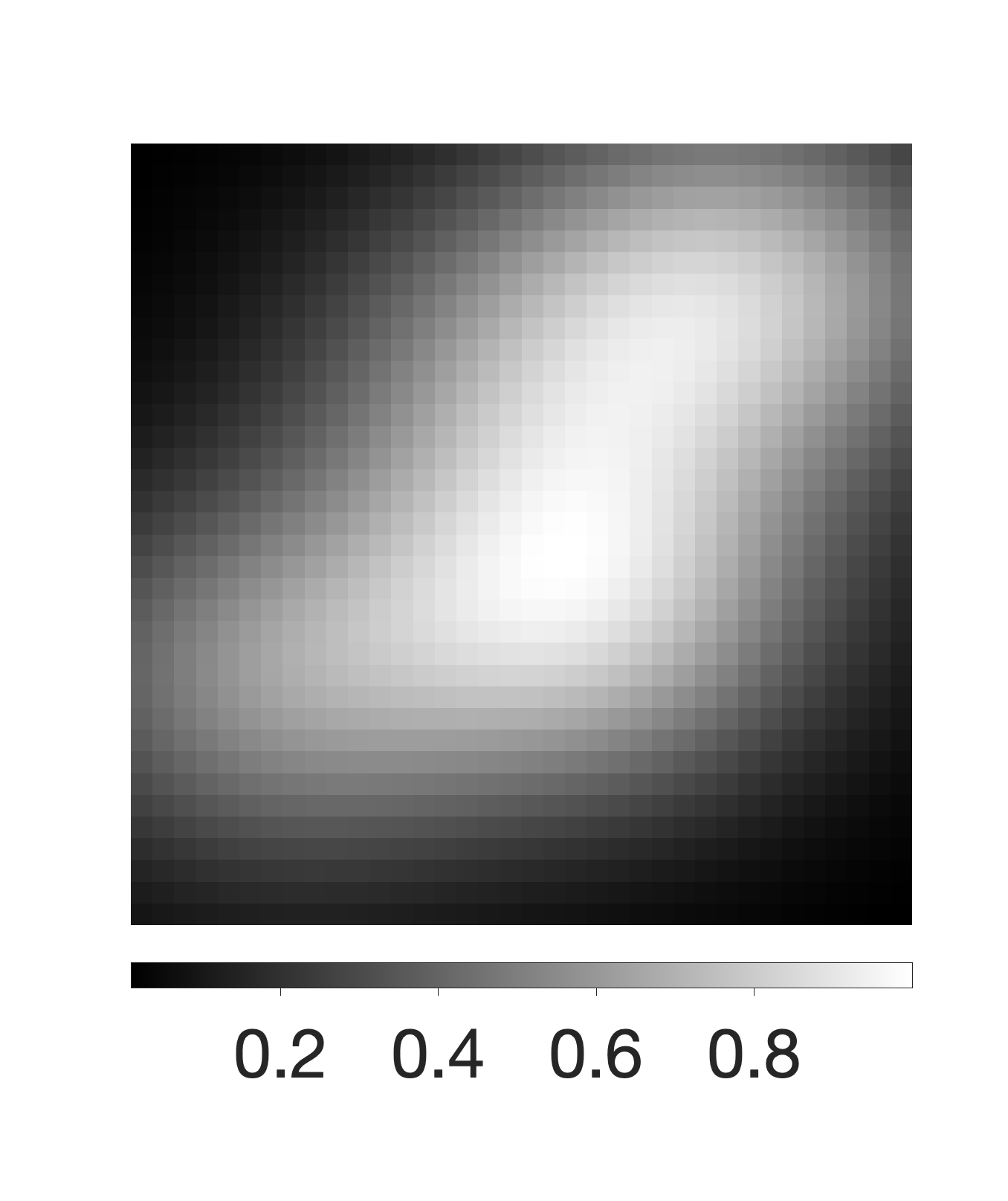
Figure 1: True reconstruction for $36\times 36$ PRspherical seismic tomography test problem

500 Samples using Metropolis-Hastings within Gibbs: genGK
$k$	acc.	Mean	Variance	$\lambda$	$\delta$
500	83
750	334
1,000	493

Table 1: Results for $T=500$ samples using Algorithm 3 on a PRspherical test problem.The proposed distribution $g_{1}({\bf x})$ uses genGK for the approximate covariance matrix ${\bm{\Gamma}}$. In column 1, $k$ denotes the rank of $\widehat{\bm{\Gamma}}$ and the second column provides the number of accepted samples. The mean and variance represent the mean and variance of all accepted samples after burn-in. The $\lambda$ and $\delta$ distributions contain all draws from $\pi_{\lambda}$ and $\pi_{\delta}$ after burn-in.

$\lambda$ Chain Analysis for 500 Samples using Metropolis-Hastings within Gibbs: genGK
$k$	p-value	ESS	$\lambda$ Samples	Autocorrelation
500	.98	193.23
750	.99	331.2
1,000	.99	338.48

Table 2: Analysis of $\lambda$ chain for $T=500$ samples using Algorithm 3 on a PRspherical test problem. Here, $k$ denotes the rank of $\widehat{\bm{\Gamma}}$, p-value gives the probablity of accepting or rejecting the Geweke null hypothesis and ESS provides essential sample size. Then, $\lambda$ Samples gives a plot of the sample value of $\lambda^{j}$ and the last column plots the autocorrelation function.

$\delta$ Chain Analysis for 500 Samples using Metropolis-Hastings within Gibbs: genGK
$k$	p-value	ESS	$\delta$ Samples	Autocorrelation
500	.91	11.63
750	.88	83.12
1,000	.96	94.21

Table 3: Analysis of $\delta$ chain for $T=500$ samples using Algorithm 3 on a PRspherical test problem. Here, $k$ denotes the rank of $\widehat{\bm{\Gamma}}$, p-value gives the probablity of accepting or rejecting the Geweke null hypothesis and ESS provides essential sample size. Then, $\delta$ Samples gives a plot of the sample value of $\delta^{j}$ and the last column plots the autocorrelation function.

Since this problem is small enough such that we can compute the singular value decomposition (SVD), we also compare to the Metropolis-Hastings within Gibbs method with low-rank proposal sampling given by truncated SVD (TSVD) and randomized SVD (rSVD) approximations with ranks of 500, 750, and 1,000. Details for using these alternative methods can be found in Appendix D. In Table 4 and Table 5 we provide the number of accepted samples, as well as the mean and variance image for ${\bf x}$ and the $\lambda$ and $\delta$ distributions using TSVD and rSVD approximations respectively. Compared with the results in Table 1, we observe that the number of accepted samples for genGK is higher than that for rSVD and slightly lower than that for SVD. However, the mean and variance image for ${\bf x}$ and the $\lambda$ and $\delta$ distributions are all very similar. In each experiment, 450 samples after burn-in are used to compute the means and variances.

500 Samples using Metropolis-Hastings within Gibbs: TSVD
$k$	acc.	Mean	Variance	$\lambda$	$\delta$
500	179
750	458
1,000	499

Table 4: Results for $T=500$ samples using Algorithm 2 on a PRspherical test problem. The proposed distribution $g_{1}({\bf x})$ uses the TSVD for the approximate covariance matrix ${\bm{\Gamma}}$. In column 1, $k$ denotes the rank of $\widehat{\bm{\Gamma}}$ and the second column provides the number of accepted samples. The mean and variance represent the mean and variance of all accepted samples after burn-in. The $\lambda$ and $\delta$ distributions contain all draws from $\pi_{\lambda}$ and $\pi_{\delta}$ after burn-in.

500 Samples using Metropolis-Hastings within Gibbs: rSVD
$k$	acc.	Mean	Variance	$\lambda$	$\delta$
500	15
750	217
1,000	462

Table 5: Results for $T=500$ samples using Algorithm 2 on a PRspherical test problem. The proposed distribution $g_{1}({\bf x})$ uses the rSVD for the approximate covariance matrix ${\bm{\Gamma}}$. In column 1, $k$ denotes the rank of $\widehat{\bm{\Gamma}}$ and the second column provides the number of accepted samples. The mean and variance represent the mean and variance of all accepted samples after burn-in. The $\lambda$ and $\delta$ distributions contain all draws from $\pi_{\lambda}$ and $\pi_{\delta}$ after burn-in.

4.2 Atmospheric Inverse Modeling

Now we consider an atmospheric transport problem where ${\bf A}\in\mathbb{R}^{98,880\times 3,222}$ represents a forward atmospheric transport model from NOAA’s CarbonTracker-Lagrange project [21, 22] modeling simulations from the weather research and forecasting stochastic time-inverted Lagrangian transport model [23, 24] sampled at 3,222 grid locations covering North America. The goal is to approximate ${\bf x}\in\mathbb{R}^{3,222}$, the vectorized true average fluxes at the grid locations. The observations ${\bf b}\in\mathbb{R}^{98,880}$ are sampled from OCO-2 during July through mid-August 2015. For this problem, we do not use realistic CO₂ emissions. Instead, ${\bf x}_{\rm true}$ is a randomly generated vectorized emission map that is used to produce the observations ${\bf b}$. We add Gaussian white noise corresponding to a $50\%$ noise level to the observations, i.e., $\frac{\sigma\left\|{\bm{\xi}}\right\|_{2}}{\left\|{\bf A}{\bf x}_{\rm true}\right\|_{2}}=0.50$ where $\sigma$ is the standard deviation and ${\bm{\xi}}\in\mathbb{R}^{98,880}\sim\mathcal{N}\left(\bf 0,{\bf I}\right)$. Using this setup, the hyperparameter associated with the noise, $\lambda$, should converge to $\frac{1}{\sigma^{2}}\approx 64.35$ for our generated ${\bm{\xi}}$.

Let ${\bf S}\in\{0,1\}^{3,222\times 11,900}$ be the sampling matrix that extracts the 3,222 grid locations over North America from the entire $11,900\times 11,900$ grid. Then, the prior covariance matrix ${\bf Q}\in\mathbb{R}^{3,222\times 3,222}$ can be created by sampling a Matérn kernel, ${\bf Q}_{M}^{11,900\times 11,900}$, with $\nu=2.5$ and $\ell=0.05$,

$${\bf Q}={\bf S}{\bf Q}_{M}{\bf S}^{\top}.$$ (34)

We compute $T=500$ samples using the Metropolis-Hastings within Gibbs method with proposal sampling using the genGK approximation (Algorithm 3) with rank $k=750$. In Figure 2 we provide the true image along with the mean and variance images of the 450 samples after burn-in and the distributions of computed hyperparameters $\lambda$ and $\delta$. It should be noted that when plotting the variance of the solution, the colorbar is set to have a maximum value of $0.07$ to give a better representation of the variance throughout the grid by excluding the high variances found only at the boundaries. This setup produced an acceptance rate of $63\%$ and it was found that the distribution of the $\lambda$ chain converges to the true value with a $95\%$ confidence interval of $[64.06,\ 65.22]$. In Table 6, an analysis of the $\lambda$ samples shows that the chain is in equilibrium given a $p$-value of $0.99$. The ACF for $\lambda$ gives evidence that there is little to no correlation in the chain and an ESS of 308 shows most all of the accepted samples are independent. However, the $\delta$ chain produced a smaller $p$-value and ESS than $\lambda$. Combined with a slower ACF decay, the $\delta$ samples from Algorithm 3 are more dependent and potentially out of equilibrium. This can be seen in the plot of $\delta$ samples which follows an upward trend.

True	Mean	Variance
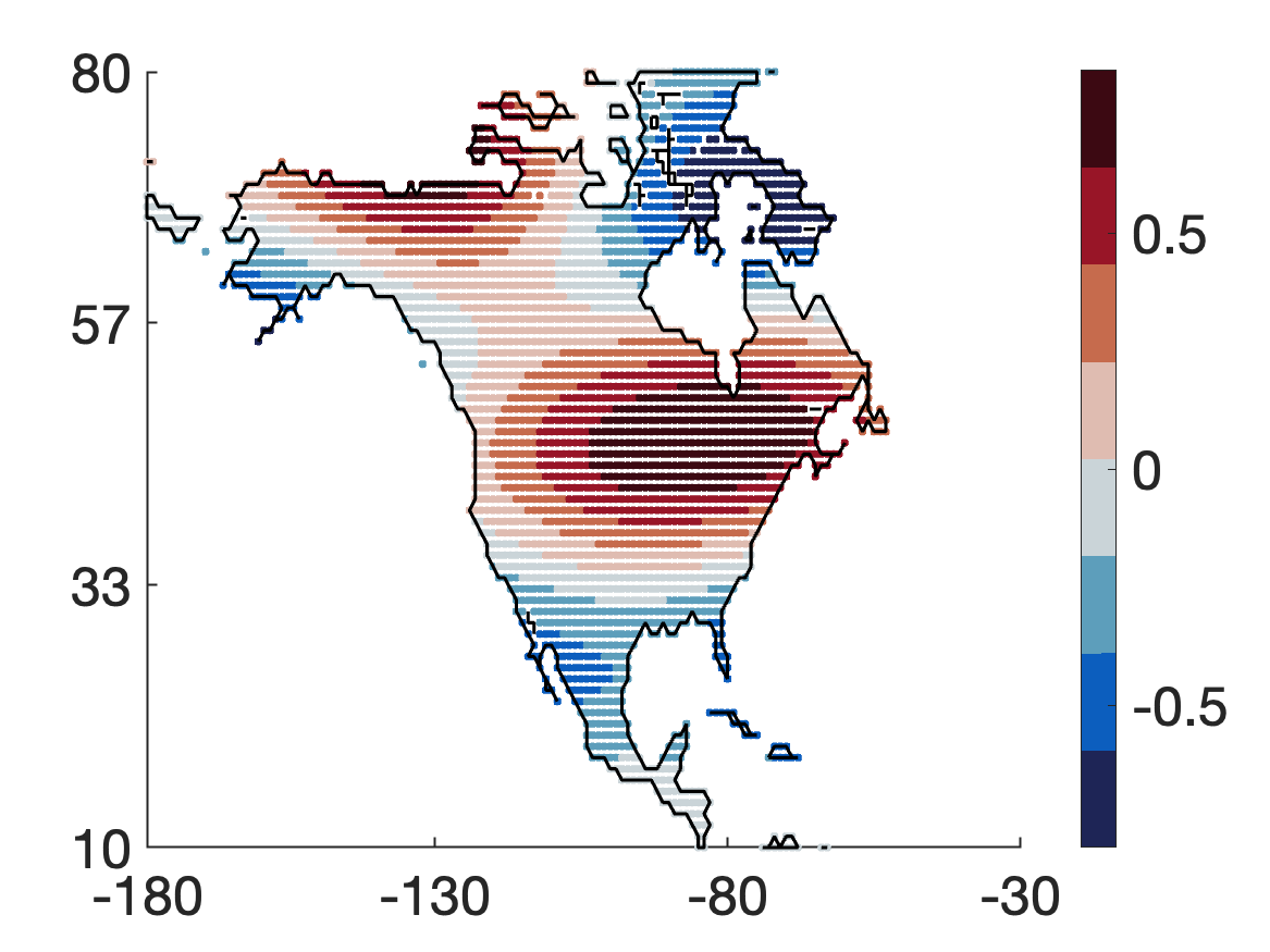
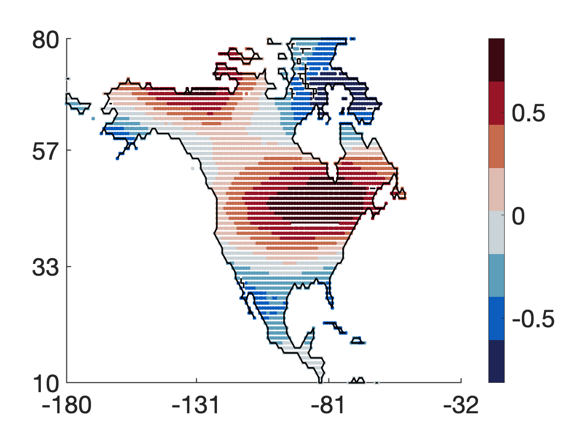
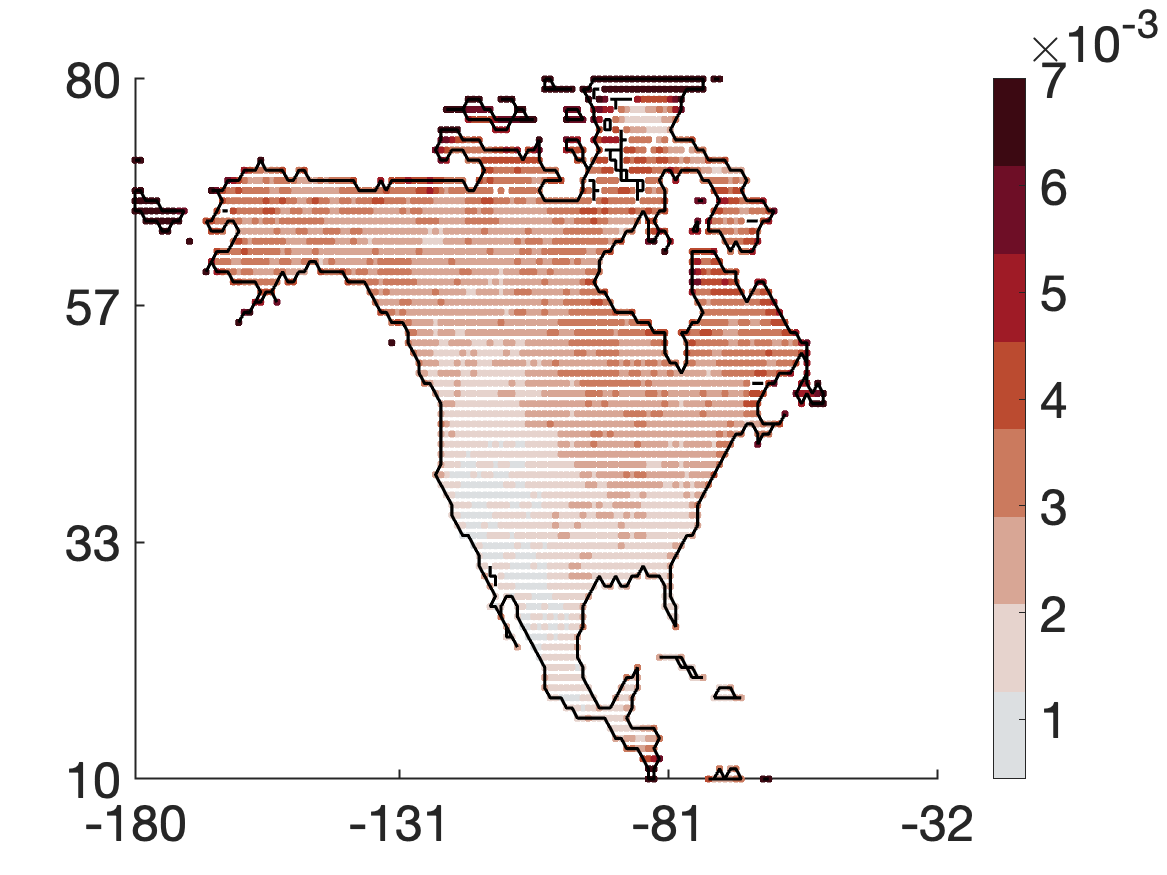
	$\lambda$ Distribution	$\delta$ Distribution

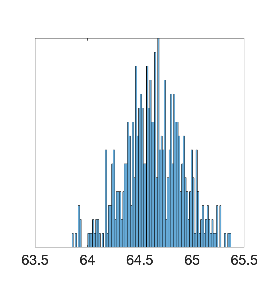
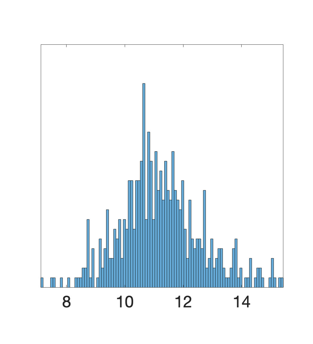
Figure 2: True atmospheric image and results for $T=500$ samples from Algorithm 3 for the atmospheric transport problem with an approximate covariance matrix of rank $k=750$. The mean and variance are taken over the 315/500 accepted samples after burn-in. The $\lambda$ and $\delta$ distributions are over all samples after burn-in.

Chain Analysis for 500 Samples using Metropolis-Hastings within Gibbs: genGK
Param.	p-value	ESS	Samples	Autocorrelation
$\lambda$	.99	308.76
$\delta$	.64	13.23

Table 6: Analysis of $\lambda$ and $\delta$ chain for $T=500$ samples using Algorithm 3 on the Atmospheric transport problem with a rank of $k=750$. Here, p-value gives the probablity of accepting or rejecting the Geweke null hypothesis and ESS provides essential sample size. Samples gives a plot of the hyperparameter values at the $j^{th}$ sample and the last column plots the autocorrelation function.

4.3 Dynamic Photoacoustic Tomography

Here we consider a dynamic photoacoustic tomography test problem, based on the PRspherical example in IRTools[20]. For this example, 20 $64\times 64$ true images were generated using two Gaussians moving in different directions. Such problems require a spatiotemporal prior, and we use a Kronecker product ${\bf Q}={\bf Q}_{t}\otimes{\bf Q}_{s}\in\mathbb{R}^{81,920\times 81,920}$ where ${\bf Q}_{t}\in\mathbb{R}^{20\times 20}$ and ${\bf Q}_{s}\in\mathbb{R}^{4,096\times 4,096}$ are temporal and spatial priors corresponding to Matérn kernels with $\nu=2.5,\ \ell=0.1$ and $\nu=0.5,\ \ell=0.25$ respectively. The linear problem can be formed by combining the subproblem at each time point $i$ as follows,

$${\bf x}=\begin{bmatrix}{\bf x}_{1}\\ \vdots\\ {\bf x}_{20}\end{bmatrix},\quad{\bf A}=\begin{bmatrix}{\bf A}_{1}&&\\ &\ddots&\\ &&{\bf A}_{20}\end{bmatrix},\quad\text{and}\quad{\bf b}=\begin{bmatrix}{\bf b}_{1}\\ \vdots\\ {\bf b}_{20}\end{bmatrix},$$

where ${\bf A}_{i}\in\mathbb{R}^{1,638\times 4,096}$ is a spherical projection matrix corresponding to 18 equally spaced angles between $i$ and $340+i$ for $i=1,\ldots,20$, ${\bf x}_{i}\in\mathbb{R}^{4,096}$ is the vectorized image at $i$, and ${\bf b}_{i}\in\mathbb{R}^{1,638}$ is the simulated projection data. We add Gaussian white noise corresponding to a $2\%$ noise level to the observations, i.e., $\frac{\sigma\left\|{\bm{\xi}}\right\|_{2}}{\left\|{\bf A}{\bf x}_{\rm true}\right\|_{2}}=0.02$ where $\sigma$ is the standard deviation and ${\bm{\xi}}\sim\mathcal{N}\left(\bf 0,{\bf I}\right)$. Using this setup, the hyperparameter associated with the noise, $\lambda$, should be $\frac{1}{\sigma^{2}}\approx 2.02\times 10^{4}$. Given the small size of ${\bf Q}_{t}$, we can obtain the Cholesky factorization ${\bf Q}_{t}^{-1}={\bf G}_{t}^{\top}{\bf G}_{t}$. Now we can define a preconditioner of the form ${\bf G}={\bf G}_{t}\otimes{\bf G}_{s}$ with ${\bf G}_{s}$ being the Cholesky factorization of $(-\Delta)^{\gamma}$ for $\gamma\geq 1$ where $\Delta$ the Laplacian operator discretized using finite difference.

The goal is this problem is to obtain a sequence of images from a sequence of projection datasets. Figure 3 contains the true image for 5 time points. We used a genGK approximation to the target distribution, but due to the large rank of this problem, the proposal failed to accept a sufficient number of samples without taking $k$ to be very large. Thus, we used the preconditioned Lanczos method from Algorithm 4. In Figure 4 we provide the results for $T=500$ samples. The approximate mean, ${\bf x}_{k}$, is obtained using $k=$1,000 genGK iterations. Additionally, the corresponding $\lambda$ and $\delta$ distributions are given in Figure 5. We also provide a sample from the prior. We observe that the method produced a $100\%$ acceptance rate. While this is higher than that of the previous examples, it is expected given an exact factorization of ${\bm{\Gamma}}_{\rm cond}$ is used. While the $\lambda$ distribution approaches the true value, it is outside the $95\%$ confidence interval of $[19,341.09,\ 20,057.78]$. This might be improved by increasing the rank of the approximate mean ${\bf x}_{k}$, but the magnitude of the hyperparameter could potentially make converging to the true value more difficult.

In Table 7 we provide an analysis of the $\lambda$ and $\delta$ chains and observe that Algorithm 4 produces samples of $\lambda$ and $\delta$ that have $p$-values of .99 providing strong evidence the chains are in equilibrium. The ACFs corresponding to both $\lambda$ and $\delta$ quickly decay to 0 so the chains are highly uncorrelated. Finally, from the ESS we see that a majority of the $\lambda$ and $\delta$ samples are independent. In comparison with the previous two examples, Algorithm 4 produced a better $\delta$ chain.

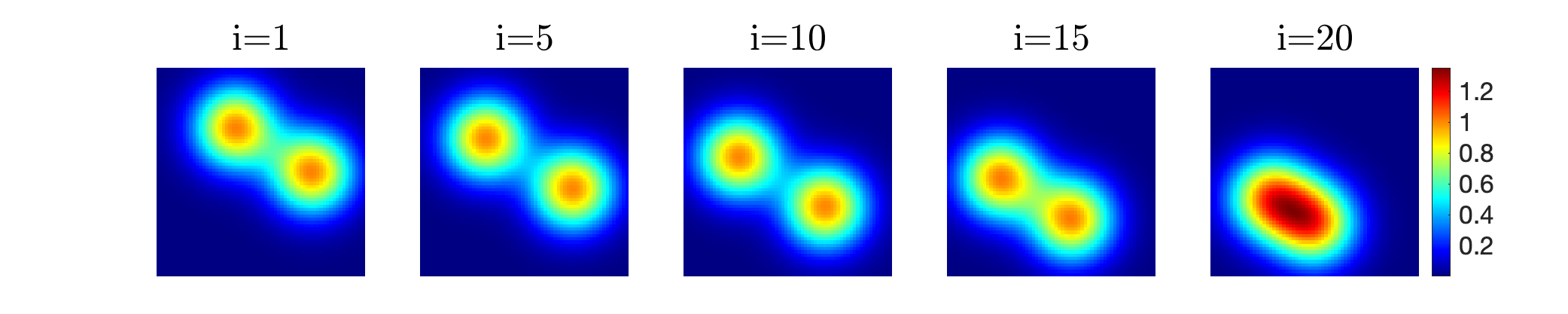
Figure 3: True $64\times 64$ images for the dynamic photoacoustic tomography problem at time points $i=1,5,10,15,\rm and\ 20$.

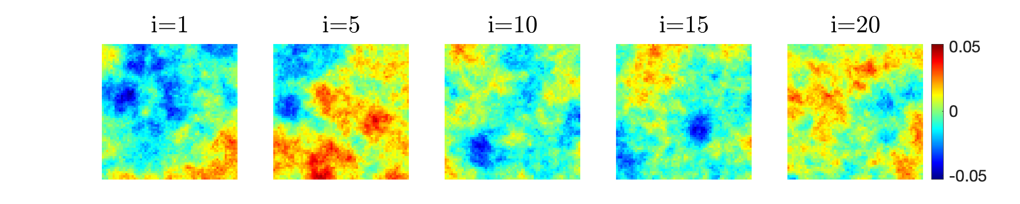
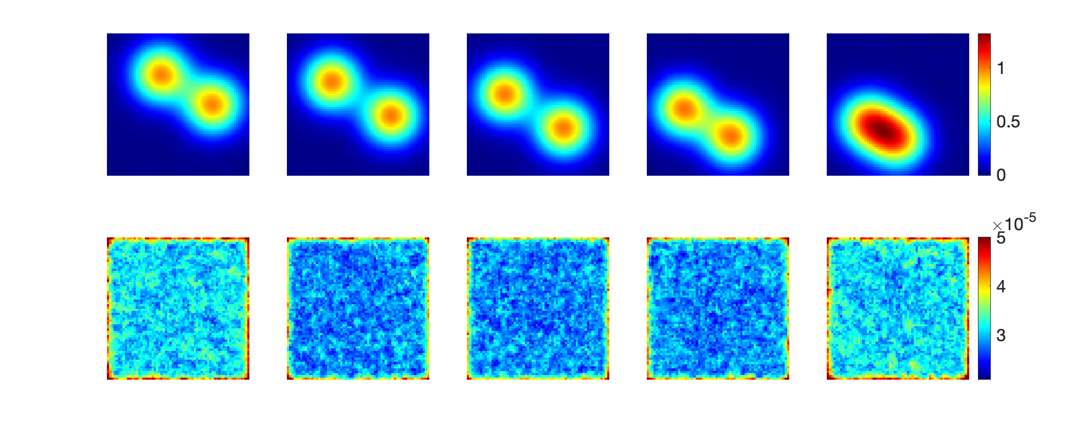
Figure 4: Results for 500/500 accepted samples from Algorithm 4 for the dynamic photoacoustic tomography test problem with an approximate mean with $k=1,000$ genGK iterations for time points $i=1,5,10,15,$ and $20$. Top: Random sample from the prior. Middle: Means of accepted samples after burn-in. Bottom: Variances of accepted samples after burn-in.

$\lambda$ Distribution	$\delta$ Distribution

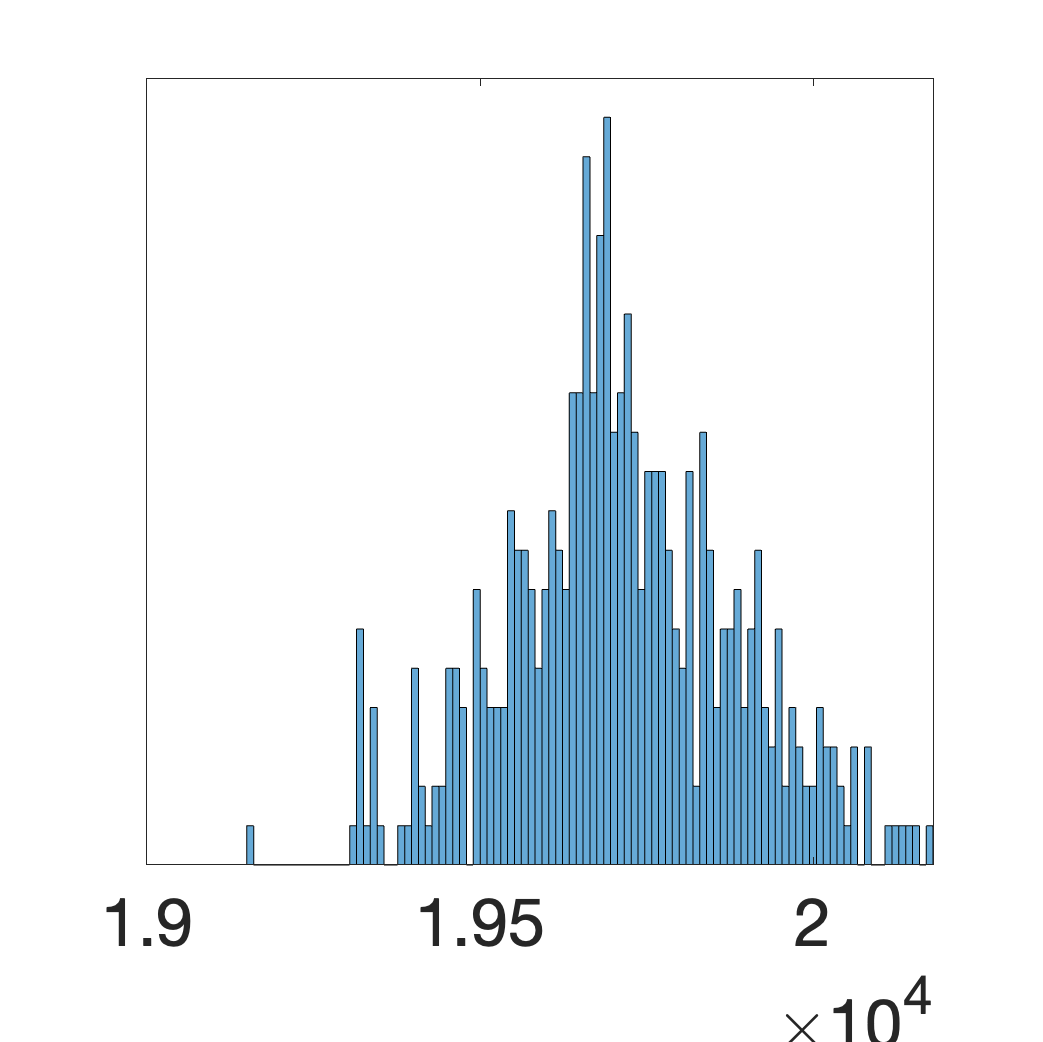
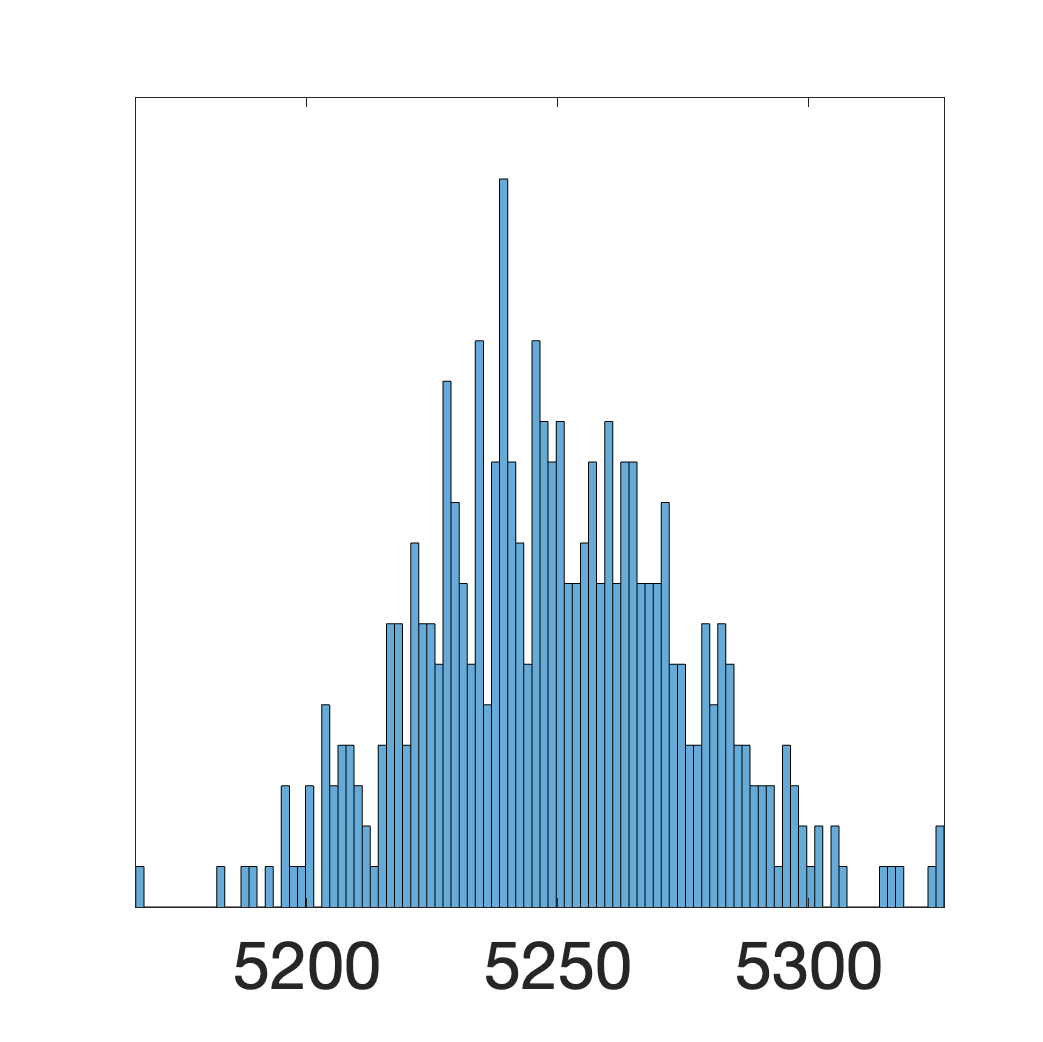
Figure 5: $\lambda$ and $\delta$ distributions of $T=500$ samples from Algorithm 4 for the dynamic photoacoustic tomography test problem with an approximate mean with $k=1,000$ genGK iterations

Chain Analysis for $500$ Samples using Metropolis-Hastings within Gibbs: genGK
Param.	p-value	ESS	Samples	Autocorrelation
$\lambda$	.99	292.77
$\delta$	.99	365.99

Table 7: Analysis of $\lambda$ and $\delta$ chain for $T=500$ samples using Algorithm 4 photoacoustic tomography test problem with an approximate mean using $k=1,000$ genGK iterations. Here, p-value gives the probablity of accepting or rejecting the Geweke null hypothesis and ESS provides essential sample size. Samples gives a plot of the hyperparameter values at the $j^{th}$ sample and the last column plots the autocorrelation function.

5 Conclusions

This paper provides an approach to perform uncertainty quantification for large-scale hierarchical Bayesian inverse problems, where Metropolis-Hastings independence sampling within Gibbs is used to overcome the limitations of Markov chain Monte Carlo methods. We consider two proposal distributions, both of which are based on generalized Golub-Kahan methods. First, using a genGK based approach to form an approximation of the distribution, we are able to reuse the genGK matrices to efficiently draw samples by forming a low-rank approximation to the conditional covariance matrix. Second, for matrices where a low-rank approximation is not sufficient, we describe a preconditioned Lanczos based method to efficiently perform computations with the square-root of the conditional covariance to draw proposal samples. In addition to comparisons with existing approaches for small problems, we demonstrate the performance of these methods on a variety of large-scale inverse problems, including atmospheric models and dynamic tomography problems.

Statements and Declarations

• Funding: This work was partially supported by the National Science Foundation program under grants DMS-2411197 and DMS-2038118. Any opinions, findings, conclusions or recommendations expressed in this material are those of the author(s) and do not necessarily reflect the views of the National Science Foundation.

• Conflict of interest/Competing interests: On behalf of all authors, the corresponding author states that there is no conflict of interest.

• Ethics approval and consent to participate: Not applicable

• Consent for publication: Not applicable

• Data availability: Not applicable

• Materials availability: Not applicable

• Code availability: Not applicable

• Author contribution: Both authors contributed equally to this work.

Appendix A Low-Rank Representation of Square-Root Covariance

First note that operations with the square-root matrix ${\bf Q}^{1/2}$ can be performed efficiently, using a Lanczos algorithm that only requires mat-vecs with ${\bf Q}$, see [14] and references therein. Next recall after $k$ iterations of the genGK bidiagonalization process, we have

$${\bf Q}^{1/2}{\bf A}^{\top}{\bf R}^{-1}{\bf A}{\bf Q}^{1/2}\approx{\bf Q}^{1/2}{\bf V}_{k}{\bf B}_{k}^{\top}{\bf B}_{k}{\bf V}_{k}^{\top}{\bf Q}^{1/2}.$$

Let ${\bf Q}^{(1)}{\bf R}^{(1)}={\bf B}_{k}$ and ${\bf Q}^{(2)}{\bf R}^{(2)}={\bf Q}^{1/2}{\bf V}_{k}({\bf R}^{(1)})^{\top}$ be QR decompositions, then

$${\bf Q}^{1/2}{\bf V}_{k}{\bf B}_{k}^{\top}{\bf B}_{k}{\bf V}_{k}^{\top}{\bf Q}^{1/2} ={\bf Q}^{(2)}{\bf R}^{(2)}({\bf R}^{(2)})^{\top}({\bf Q}^{(2)})^{\top}.$$

Taking the eigenvalue decomposition ${\bf R}^{(2)}({\bf R}^{(2)})^{\top}={\bf W}_{k}\mathbf{\Theta}_{k}{\bf W}_{k}^{\top}$ and assigning ${\bf Z}_{k}={\bf Q}^{(2)}{\bf W}_{k}$, we get the low-rank representation,

$${\bf Q}^{1/2}{\bf A}^{\top}{\bf R}^{-1}{\bf A}{\bf Q}^{1/2}\approx{\bf Z}_{k}\mathbf{\Theta}_{k}{\bf Z}_{k}\quad\text{where}\quad\mathbf{\Theta}_{k}={\rm diag\!}\left([\theta_{1},\ldots,\theta_{k}]\right).$$ (35)

To compute the inverse square-root $\left(\delta{\bf I}+\lambda{\bf Q}^{1/2}{\bf A}^{\top}{\bf R}^{-1}{\bf A}{\bf Q}^{1/2}\right)^{-1/2}$, following [7], we use the Woodbury identity to get

$$\left(\delta{\bf I}+\lambda{\bf Q}^{1/2}{\bf A}^{\top}{\bf R}^{-1}{\bf A}{\bf Q}^{1/2}\right)^{-1} =\delta^{-1}\left({\bf I}+{\bf Z}_{k}(\lambda/\delta)\mathbf{\Theta}_{k}{\bf Z}_{k}^{\top}\right)^{-1}$$

$$=\delta^{-1}\left({\bf I}-{\bf Z}_{k}\left({\bf I}_{k}+(\lambda/\delta)^{-1}\mathbf{\Theta}_{k}^{-1}\right)^{-1}{\bf Z}_{k}^{\top}\right).$$

Then we can compute a square-root matrix as

$$\delta^{-1/2}\left({\bf I}+{\bf Z}_{k}(\lambda/\delta)\mathbf{\Theta}_{k}{\bf Z}_{k}^{\top}\right)^{-1/2} =\delta^{-1/2}\left({\bf I}_{n}-{\bf Z}_{k}{\bf D}_{k}{\bf Z}_{k}^{\top}\right)$$ (36)

where ${\bf D}_{k}\equiv{\bf I}_{k}-\left((\lambda/\delta)\mathbf{\Theta}_{k}+{\bf I}_{k}\right)^{-1/2}$.

Appendix B Prior norm for genGK proposal

To evaluate $\left\|{\bf x}^{t-1}\right\|_{{\bf Q}^{-1}}^{2}$, we use an equivalent expression that avoids computations with ${\bf Q}^{-1}$. Let ${\bf x}_{k}={\bf Q}{\bf V}_{k}{\bf z}_{k}$ be the genGK approximation used as the mean of the distribution from which ${\bf x}^{t-1}$ was drawn and ${\bf D}_{k}$ be the matrix used to form the corresponding $\widehat{\bm{\Gamma}}_{\rm cond}^{1/2}$. Then, the norm can be written as

$$\left\|{\bf x}^{t-1}\right\|_{{\bf Q}^{-1}}^{2}$$

$$=\left({\bf x}^{t-1}\right)^{\top}{\bf Q}^{-1}\left({\bf x}^{t-1}\right)$$

$$=\left({\bf Q}{\bf V}_{k}{\bf z}_{k}+\frac{{\bf Q}^{1/2}}{\sqrt{\delta}}\left({\bf I}-{\bf Z}_{k}{\bf D}_{k}{\bf Z}_{k}^{\top}\right){\bm{\xi}}\right)^{\top}{\bf Q}^{-1}\left({\bf Q}{\bf V}_{k}{\bf z}_{k}+\frac{{\bf Q}^{1/2}}{\sqrt{\delta}}\left({\bf I}-{\bf Z}_{k}{\bf D}_{k}{\bf Z}_{k}^{\top}\right){\bm{\xi}}\right)$$

$$=\left({\bf Q}^{1/2}{\bf V}_{k}{\bf z}_{k}+\delta^{-1/2}\left({\bf I}-{\bf Z}_{k}{\bf D}_{k}{\bf Z}_{k}^{\top}\right){\bm{\xi}}\right)^{\top}\left({\bf Q}^{1/2}{\bf V}_{k}{\bf z}_{k}+\delta^{-1/2}\left({\bf I}-{\bf Z}_{k}{\bf D}_{k}{\bf Z}_{k}^{\top}\right){\bm{\xi}}\right)$$

$$=\left(({\bf V}_{k}{\bf z}_{k})^{\top}{\bf Q}^{1/2}+\delta^{-1/2}{\bm{\xi}}^{\top}\left({\bf I}-{\bf Z}_{k}{\bf D}_{k}{\bf Z}_{k}^{\top}\right)\right)\left({\bf Q}^{1/2}{\bf V}_{k}{\bf z}_{k}+\delta^{-1/2}\left({\bf I}-{\bf Z}_{k}{\bf D}_{k}{\bf Z}_{k}^{\top}\right){\bm{\xi}}\right)$$

so finally we have

$$\left\|{\bf x}^{t-1}\right\|_{{\bf Q}^{-1}}^{2}=\left({\bf V}_{k}{\bf z}_{k}\right)^{\top}({\bf x}_{k}+2\widehat{\bm{\Gamma}}_{\rm cond}^{1/2}{\bm{\xi}})+{\bm{\xi}}^{\top}\delta^{-1}\left({\bf I}-{\bf Z}_{k}\left(({\bf D}_{k})^{2}-2{\bf D}_{k}\right){\bf Z}_{k}^{\top}\right){\bm{\xi}}.$$ (37)

Appendix C Derivation of acceptance ratio and prior norm for Section 3.3

Let ${\bf x}_{k}$ be the genGK approximation used as the mean of the distribution from which ${\bf x}^{t-1}$ was drawn. Consider the log of the full acceptance ratio,

$$\log\alpha_{2}({\bf x}^{t-1},{\bf x}^{\star})$$

$$\quad=-\frac{1}{2}\Big{(}({\bf x}^{\star}-{\bf x}_{\rm cond})^{\top}{\bm{\Gamma}}_{\rm cond}^{-1}({\bf x}^{\star}-{\bf x}_{\rm cond})+({\bf x}^{t-1}-{\bf x}_{k})^{\top}{\bm{\Gamma}}_{\rm cond}^{-1}({\bf x}^{t-1}-{\bf x}_{k})$$

$$\qquad-({\bf x}^{t-1}-{\bf x}_{\rm cond})^{\top}{\bm{\Gamma}}_{\rm cond}^{-1}({\bf x}^{t-1}-{\bf x}_{\rm cond})+({\bf x}^{\star}-{\bf x}_{k})^{\top}{\bm{\Gamma}}_{\rm cond}^{-1}({\bf x}^{\star}-{\bf x}_{k})\Big{)}$$

$$\quad={\bf x}_{\rm cond}^{\top}{\bm{\Gamma}}_{\rm cond}^{-1}{\bf x}^{\star}+{\bf x}_{k}^{\top}{\bm{\Gamma}}_{\rm cond}^{-1}{\bf x}^{t-1}-{\bf x}_{\rm cond}^{\top}{\bm{\Gamma}}_{\rm cond}^{-1}{\bf x}^{t-1}-{\bf x}_{k}^{\top}{\bm{\Gamma}}_{\rm cond}^{-1}{\bf x}^{\star},$$

after expanding and canceling like terms. Using ${\bf x}_{\rm cond}=\lambda{\bm{\Gamma}}_{\rm cond}{\bf A}^{\top}{\bf R}^{-1}{\bf b}$, ${\bm{\Gamma}}_{\rm cond}^{-1}=\lambda{\bf A}^{\top}{\bf R}^{-1}{\bf A}+\delta{\bf Q}^{-1}$, and ${\bf x}_{k}={\bf Q}{\bf V}_{k}{\bf z}_{k}$, the equation reduces to

$$\log\alpha_{2}({\bf x}^{t-1},{\bf x}^{\star}) =\lambda({\bf A}^{\top}{\bf R}^{-1}{\bf b})^{\top}{\bf x}^{\star}+(\lambda{\bf x}_{k}^{\top}{\bf A}^{\top}{\bf R}^{-1}{\bf A}+\delta({\bf V}_{k}{\bf z}_{k})^{\top}){\bf x}^{t-1}$$

$$\quad-\lambda({\bf A}^{\top}{\bf R}^{-1}{\bf b})^{\top}{\bf x}^{t-1}-(\lambda{\bf x}_{k}^{\top}{\bf A}^{\top}{\bf R}^{-1}{\bf A}+\delta({\bf V}_{k}{\bf z}_{k})^{\top}){\bf x}^{\star}$$

$$=\left({\bf x}^{\star}-{\bf x}^{t-1}\right)^{\top}\left(\lambda{\bf A}^{\top}{\bf R}^{-1}\left({\bf b}-{\bf A}{\bf x}_{k}\right)-\delta{\bf V}_{k}{\bf z}_{k}\right)$$

$$=\left({\bf x}^{\star}-{\bf x}^{t-1}\right)^{\top}\left(\lambda\left(\gamma_{1}\alpha_{1}{\bf v}_{1}-{\bf V}_{k+1}\begin{bmatrix}{\bf B}_{k}^{\top}\\ \alpha_{k+1}{\bf e}_{k+1}^{\top}\end{bmatrix}{\bf B}_{k}{\bf z}_{k}\right)-\delta{\bf V}_{k}{\bf z}_{k}\right).$$

Note that

$${\bf V}_{k+1}\begin{bmatrix}{\bf B}_{k}^{\top}\\ \alpha_{k+1}{\bf e}_{k+1}^{\top}\end{bmatrix}{\bf B}_{k}{\bf z}_{k}={\bf V}_{k}{\bf b}_{k}^{\top}{\bf B}_{k}{\bf z}_{k}+\alpha_{k+1}\gamma_{k+1}\left({\bf e}_{k}^{\top}{\bf z}_{k}\right){\bf v}_{k+1}.$$ (38)

Next, to avoid ${\bf Q}^{-1}$ when computing $\left\|{\bf x}^{t-1}\right\|_{{\bf Q}^{-1}}^{2}$, notice that the norm can be equivalently written as

$$\left\|{\bf x}^{t-1}\right\|_{{\bf Q}^{-1}}^{2} =\left({\bf x}^{t-1}\right)^{\top}{\bf Q}^{-1}\left({\bf x}^{t-1}\right)$$

$$=\left({\bf x}^{t-1}\right)^{\top}{\bf Q}^{-1}\left({\bf x}_{k}+{\bf S}_{F}{\bm{\xi}}\right)$$

$$=\left({\bf x}^{t-1}\right)^{\top}{\bf Q}^{-1}\left({\bf Q}{\bf V}_{k}{\bf z}_{k}+\lambda^{-1/2}{\bf Q}{\bf G}^{\top}\left({\bf G}{\bf F}{\bf G}^{\top}\right)^{-1/2}{\bm{\xi}}\right)$$

where ${\bf F}=\frac{\delta}{\lambda}{\bf Q}+{\bf Q}{\bf A}^{\top}{\bf R}^{-1}{\bf A}{\bf Q}$. Distributing ${\bf Q}^{-1}$ results in

$$\left\|{\bf x}^{t-1}\right\|_{{\bf Q}^{-1}}^{2}=\left({\bf x}^{t-1}\right)^{\top}\left({\bf V}_{k}{\bf z}_{k}+\lambda^{-1/2}{\bf G}^{\top}\left({\bf G}{\bf F}{\bf G}^{\top}\right)^{-1/2}{\bm{\xi}}\right)$$ (39)

which reuses the previously computed ${\bf V}_{k}{\bf z}_{k}$ and ${\bf G}^{\top}\left({\bf G}{\bf F}{\bf G}^{\top}\right)^{-1/2}{\bm{\xi}}$.

Appendix D SVD and rSVD approximations of the conditional covariance matrix

Assume the factorization ${\bf Q}={\bf L}^{\top}{\bf L}$ is accessible. Then, for fixed $\lambda$ and $\delta$,

$${\bm{\Gamma}}_{\rm cond} =\left(\delta{\bf L}^{-1}{\bf L}^{-\top}+\lambda{\bf A}^{\top}{\bf R}^{-1}{\bf A}\right)^{-1}$$

$$={\bf L}^{\top}\left(\delta{\bf I}+\lambda{\bf L}{\bf A}^{\top}{\bf R}^{-1}{\bf A}{\bf L}^{\top}\right)^{-1}{\bf L}.$$

To form a low-rank approximation of ${\bf H}={\bf L}{\bf A}^{\top}{\bf R}^{-1}{\bf A}{\bf L}^{\top}$, we consider two approaches.

One approach is to use the truncated SVD (TSVD) where a rank $k$ approximation is formed by computing ${\bf R}^{-1/2}{\bf A}{\bf L}^{\top}\approx\widehat{\bf U}_{k}{\bm{\Sigma}}_{k}\widehat{\bf V}_{k}$ where $\widehat{\bf U}_{k}\in\mathbb{R}^{m\times k}$ and $\widehat{\bf V}_{k}\in\mathbb{R}^{n\times k}$ are orthonormal matrices containing the first $k$ left and right singular vectors of ${\bf R}^{-1/2}{\bf A}{\bf L}^{\top}$ respectively and ${\bm{\Sigma}}_{k}\in\mathbb{R}^{k\times k}$ is a diagonal matrix with the first $k$ largest singular values. Then ${\bf H}\approx\widehat{\bf V}_{k}{\bm{\Sigma}}^{2}_{k}\widehat{\bf V}_{k}^{\top}$.

Another approach is to use the randomized SVD (rSVD) algorithm which begins by using a random matrix ${\bm{\Omega}}\in\mathbb{R}^{n\times(k+p)}$ whose entries are realizations of i.i.d. standard Gaussian random variables to approximate the column space of ${\bf H}$, i.e., ${\bf Y}={\bf H}{\bm{\Omega}}$. Here $k$ is the target rank and $p$ is an oversampling parameter usually taken to be a small integer ($p=5$ or $p=10$). Compute a thin-QR factorization, ${\bf Y}=\widehat{\bf Q}\widehat{\bf R}$. Now an approximation of ${\bf H}$ is given by

$${\bf H}\approx\widehat{\bf Q}\widehat{\bf Q}^{\top}{\bf H}\widehat{\bf Q}\widehat{\bf Q}^{\top}=\widehat{\bf Q}\tilde{{\bf U}}\tilde{{\bm{\Sigma}}}\tilde{{\bf U}}^{\top}\widehat{\bf Q}^{\top}=\tilde{{\bf V}}\tilde{{\bm{\Sigma}}}\tilde{{\bf V}}^{\top}$$

where $\widehat{\bf Q}^{\top}{\bf H}\widehat{\bf Q}=\tilde{{\bf U}}\tilde{{\bm{\Sigma}}}\tilde{{\bf U}}^{\top}$ is an eigendecomposition and $\tilde{{\bf V}}=\widehat{\bf Q}\tilde{{\bf U}}$.

For both methods, the approximation of ${\bf H}$ can be used to form a low-rank representation of ${\bm{\Gamma}}_{\rm cond}$ following a similar approach to the one in Section 3.2. Using the rSVD approximation as a proposal sampler was considered in [25].

References

- \bibcommenthead
- Chung and Gazzola [2024] Chung, J., Gazzola, S.: Computational methods for large-scale inverse problems: a survey on hybrid projection methods. SIAM Review 66(2), 205–284 (2024)
- Cho et al. [2022] Cho, T., Chung, J., Miller, S.M., Saibaba, A.K.: Computationally efficient methods for large-scale atmospheric inverse modeling. Geoscientific Model Development 15(14), 5547–5565 (2022)
- Pasha et al. [2023] Pasha, M., Saibaba, A.K., Gazzola, S., Español, M.I., de Sturler, E.: A computational framework for edge-preserving regularization in dynamic inverse problems. Electronic Transactions on Numerical Analysis 58, 486–516 (2023)
- Chung et al. [2018] Chung, J., Saibaba, A.K., Brown, M., Westman, E.: Efficient generalized Golub–Kahan based methods for dynamic inverse problems. Inverse Problems 34(2), 024005 (2018)
- Calvetti and Somersalo [2007] Calvetti, D., Somersalo, E.: An Introduction to Bayesian Scientific Computing: Ten Lectures on Subjective Computing vol. 2. Springer, New York (2007)
- Bardsley [2018] Bardsley, J.M.: Computational Uncertainty Quantification for Inverse Problems vol. 19. SIAM, Philadelphia (2018)
- Bui-Thanh et al. [2013] Bui-Thanh, T., Ghattas, O., Martin, J., Stadler, G.: A computational framework for infinite-dimensional Bayesian inverse problems part i: The linearized case, with application to global seismic inversion. SIAM Journal on Scientific Computing 35(6), 2494–2523 (2013)
- Bui-Thanh and Ghattas [2014] Bui-Thanh, T., Ghattas, O.: An analysis of infinite dimensional Bayesian inverse shape acoustic scattering and its numerical approximation. SIAM/ASA Journal on Uncertainty Quantification 2(1), 203–222 (2014) https://doi.org/10.1137/120894877
- Brown et al. [2018] Brown, D.A., Saibaba, A., Vallélian, S.: Low-rank independence samplers in hierarchical Bayesian inverse problems. SIAM/ASA Journal on Uncertainty Quantification 6(3), 1076–1100 (2018)
- Saibaba et al. [2020] Saibaba, A.K., Chung, J., Petroske, K.: Efficient Krylov subspace methods for uncertainty quantification in large Bayesian linear inverse problems. Numerical Linear Algebra with Applications 27(5), 2325 (2020)
- Gelman et al. [2013] Gelman, A., Carlin, J.B., Stern, H.S., Dunson, D.B., Vehtari, A., Rubin, D.B.: Bayesian Data Analysis, Third Edition. Chapman & Hall/CRC Texts in Statistical Science. Taylor & Francis, Florida (2013). https://books.google.com/books?id=ZXL6AQAAQBAJ
- Saibaba et al. [2019] Saibaba, A.K., Bardsley, J., Brown, D.A., Alexanderian, A.: Efficient marginalization-based MCMC methods for hierarchical Bayesian inverse problems. SIAM/ASA Journal on Uncertainty Quantification 7(3), 1105–1131 (2019)
- Robert and Casella [2004] Robert, C.P., Casella, G.: Monte Carlo Statistical Methods, 2nd edn. Springer, New York (2004)
- Saibaba et al. [2020] Saibaba, A., Chung, J., Petroske, K.: Efficient Krylov subspace methods for uncertainty quantification in large bayesian linear inverse problems. Numerical Linear Algebra with Applications 27 (2020) https://doi.org/10.1002/nla.2325
- Chung et al. [2018] Chung, J., Saibaba, A.K., Brown, M., Westman, E.: Efficient generalized Golub–Kahan based methods for dynamic inverse problems. Inverse Problems 34(2), 024005 (2018)
- Arioli [2013] Arioli, M.: Generalized Golub–Kahan bidiagonalization and stopping criteria. SIAM Journal on Matrix Analysis and Applications 34(2), 571–592 (2013)
- Chung and Saibaba [2017] Chung, J., Saibaba, A.K.: Generalized hybrid iterative methods for large-scale Bayesian inverse problems. SIAM Journal on Scientific Computing 39(5), 24–46 (2017)
- Hall-Hooper et al. [2024] Hall-Hooper, K.A., Saibaba, A.K., Chung, J., Miller, S.M.: Efficient iterative methods for hyperparameter estimation in large-scale linear inverse problems. Advances in Computational Mathematics 50(6), 1–33 (2024)
- Donoho [1995] Donoho, D.L.: De-noising by soft-thresholding. IEEE Transactions on Information Theory 41(3), 613–627 (1995)
- Gazzola et al. [2019] Gazzola, S., Hansen, P.C., Nagy, J.G.: IR Tools: a MATLAB package of iterative regularization methods and large-scale test problems. Numerical Algorithms 81(3), 773–811 (2019)
- Miller et al. [2020] Miller, S.M., Saibaba, A.K., Trudeau, M.E., Mountain, M.E., Andrews, A.E.: Geostatistical inverse modeling with very large datasets: an example from the orbiting carbon observatory 2 (oco-2) satellite. Geoscientific Model Development 13(3), 1771–1785 (2020) https://doi.org/10.5194/gmd-13-1771-2020
- Liu et al. [2021] Liu, X., Weinbren, A.L., Chang, H., Tadić, J.M., Mountain, M.E., Trudeau, M.E., Andrews, A.E., Chen, Z., Miller, S.M.: Data reduction for inverse modeling: an adaptive approach v1.0. Geoscientific Model Development 14(7), 4683–4696 (2021) https://doi.org/10.5194/gmd-14-4683-2021
- Lin et al. [2003] Lin, J.C., Gerbig, C., Wofsy, S.C., Andrews, A.E., Daube, B.C., Davis, K.J., Grainger, C.A.: A near-field tool for simulating the upstream influence of atmospheric observations: The stochastic time-inverted lagrangian transport (stilt) model. Journal of Geophysical Research: Atmospheres 108(D16) (2003) https://doi.org/10.1029/2002JD003161 https://agupubs.onlinelibrary.wiley.com/doi/pdf/10.1029/2002JD003161
- Nehrkorn et al. [2010] Nehrkorn, T., Eluszkiewicz, J., Wofsy, S.C., Lin, J.C., Gerbig, C., Longo, M., Freitas, S.: Coupled weather research and forecasting–stochastic time-inverted lagrangian transport (wrf–stilt) model. Meteorology and Atmospheric Physics 107, 51–64 (2010) https://doi.org/%****␣main.bbl␣Line␣400␣****10.1007/s00703-010-0068-x
- Saibaba and Vallelian [2018] Saibaba, A.K., Vallelian, S.: Low-rank independence samplers in hierarchical Bayesian inverse problems. SIAM/ASA J. Uncertain. Quantification 6, 1076–1100 (2018)