Posterior SBC: Simulation-Based Calibration Checking Conditional on Data
Abstract
Simulation-based calibration checking (SBC) refers to the validation of an inference algorithm and model implementation through repeated inference on data simulated from a generative model. In the original and commonly used approach, the generative model uses parameters drawn from the prior, and thus the approach is testing whether the inference works for simulated data generated with parameter values plausible under that prior. This approach is natural and desirable when we want to test whether the inference works for a wide range of datasets we might observe. However, after observing data, we are interested in answering whether the inference works conditional on that particular data. In this paper, we propose posterior SBC and demonstrate how it can be used to validate the inference conditionally on observed data. We illustrate the utility of posterior SBC in three case studies: (1) A simple multilevel model; (2) a model that is governed by differential equations; and (3) a joint integrative neuroscience model which is approximated via amortized Bayesian inference with neural networks.
1 Introduction

To ensure trust on the results of the inference, different forms of calibration checking play important roles in the Bayesian workflow for model building. Simulation-based calibration checking (SBC) is one of these methods and validates the chosen posterior inference algorithm as well as checks for inconsistencies between the model implementation and a possibly separate implementation of the data generating process. As the software and algorithms for probabilistic modelling advance, the threshold for specifying increasingly complicated models gets lowered. However, as the complexity of the models increases, the probability of human error during the implementation of the model increases. In addition to such implementation mistakes, the inference algorithms used for obtaining posterior approximations can work well for one posterior, but suffer from computational difficulties for another. By simply changing the observed data, one may obtain vastly different posterior geometries, favoring one implementation or algorithm over another.
SBC validates both the implementation of the model and the inference algorithm, but it is limited to checking for calibration on the whole joint distribution of parameters and observations under the specified priors. Specifying prior distributions that accurately present the available prior information is often difficult. In some cases, the prior specifications result in SBC indicating issues, when in truth these issues are limited to a region of the prior space which is of no interest to the modeller. SBC also tends to be computationally expensive, as multiple model refits are required. One can choose to save computational resources by reducing the number of refits, but this in turn also reduces the power of the calibration checking procedure. When reducing the computational budget, SBC may fail to detect problems in the posterior inference if they are infrequent on data drawn from the full prior predictive distribution. After collecting data and running inference, these issues may be present in a large proportion of plausible parameter values.
In this paper, we introduce posterior SBC, a variant of SBC validating the inference algorithm and model implementation when conditioned on some fixed set of data. First, we introduce the method of simulation-based calibration as it has traditionally been operationalized. To emphasize the distinction between these methods, we denote this traditional implementation as prior SBC. Next, in Section 2, we introduce posterior SBC. In Section 3 we illustrate the differences between prior and posterior SBC through three case studies including a simple hierarchical model, Lotka-Volterra model, and a drift-diffusion model. Finally, in section 4 we summarize the contributions of the paper and provide an outlook for future research.
1.1 Simulation-based calibration checking
Cook et al., (2006) proposed a simulation-based calibration checking method for validating Bayesian inference software. The method is based on factoring the joint distribution of data and model parameters in two ways;
| (1) |
When considering two draws, , and data , the joint distribution is
| (2) |
Above, it’s easy to see that and have the same distribution conditionally on . If we use (1) to rewrite the joint distribution in (2) as
and still have the same distribution conditionally on .
We can sample from the joint distribution by first sampling and , which is usually easy for generative models. The last step is to sample from the conditional , which is usually not trivial and requires the use of some inference algorithm, such as Markov chain Monte Carlo (MCMC). We can validate the algorithm and its implementation for sampling by checking that, conditionally on , the samples obtained have the same distribution as .
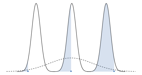
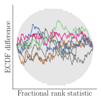
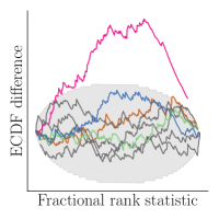
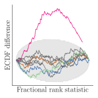
To assess whether and are from the same distribution conditional on , Cook et al., (2006) repeatedly draw parameter vectors from the prior , generate data from the observation model , and then use the algorithm to be validated to sample from the posterior . They then propose to compute empirical probability integral transform (PIT) values, , which prove to be uniformly distributed as . The process is repeated for and the empirical PIT values are used for testing. Figure 2 shows three iterations of prior draws and their respective PIT relative to the corresponding posterior distributions. Cook et al., (2006) further propose the use of the -test for the inverse of the normal cumulative distribution function (CDF) of the empirical PIT values.
Cook et al., (2006) did not take into account that the estimated PIT values are discrete when computed with finite sample size , and how the possible correlation in Markov chains affects the results (Gelman,, 2017; Talts et al.,, 2020). Talts et al., (2020) propose testing for the discrete uniformity of the empirical PIT values (see also Modrák et al.,, 2023, for improved theory and proofs). By thinning to remove possible autocorrelation, the uniformity of these discrete empirical PIT values can be tested with the approach presented in Säilynoja et al., (2022).
Instead of only assessing the uniformity of the ranks of individual parameters, Modrák et al., (2023) propose the use of the joint log-likelihood of the prior predictive sample as a test statistic for assessing the calibration. This has the additional power of detecting calibration issues rising from the model partially ignoring the data. Another advantage of this approach lies in modelling applications with high-dimensional parameter spaces, where modelers might not be particularly interested in gauging the calibration of individual parameters. Here, using the joint log-likelihood avoids the need of correcting for multiple comparisons from simultaneously assessing the calibration of all individual parameters.
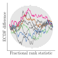
Performing SBC on the full prior parameter space has three fundamental drawbacks. First, as shown in the case study of Section 3.1, a region of calibration issues may have relatively small effect on prior SBC, but contain a relevant proportion of the posterior of some later observed dataset, thus making the results of prior SBC too optimistic for that dataset. Second, the time required for running the inference on each SBC iteration is often non-trivial and one quickly needs to consider the tradeoff between their computational budged and the power of the calibration checking. Third, as visualized in Figure 1, even with unlimited computational resources the result of prior SBC does not guarantee calibration within a specific subregion of the inspected parameter space. There can always be another region with an equally strong but reverse effect on the overall distribution of the PIT values. As proposed by Modrák et al., (2023), one solution to this last problem is to employ additional test quantities using functions of parameters and non-monotonic transformations (such as folded rank statistics), that might detect these problematic regions, but coming up with these test quantities can be difficult.
2 Posterior simulation-based calibration checking – SBC conditioned on observed data
Weakly informative priors are commonly used in Bayesian inference due to their desirable properties in real-life applications (Gelman et al.,, 2017). However, this class of priors can cause serious issues for interpreting the results of prior SBC. Even though a large portion of the prior mass may lie on a region of the parameter space where the inference works well, smaller regions may exist where the inference can fail. On the one hand, if large enough, these issues may be detected through prior SBC. The modeller could then try to modify the priors or the model to reduce the prior probability of the problematic parameter values. On the other hand, if one already has access to the data that the model will later be used to run inference on, the assessment of the inference algorithm could be focused on the region of the parameter space around the posterior. For inference on the given data, this is arguably the most important region to ensure proper calibration for.
Using the sequential Bayesian updating rule, one can view the posterior as the new prior and perform the entire SBC procedure conditional on the observed data . In other words, by conditioning the joint distribution in 2 on the observed data,
| (3) |
we see that a sample from the old posterior , and drawn from an augmented posterior, need to have the same distribution given a prediction . Thus, we operationalize the approach for data conditioned SBC by drawing , generating posterior predictions , and then using the inference algorithm to be validated to draw from the new posterior .
The validity of the algorithm can be assessed by testing the uniformity of PIT values, , this time computed for the original posterior draws, , with regard to the (thinned) augmented posterior draws, . We call this variant of SBC using posterior predictive draws posterior SBC.
When using prior SBC for validating the inference algorithm, drawing parameter values generatively from the prior is usually assumed to be trivial. In posterior SBC, we need to sample from two different posteriors, which would usually achieved using the same algorithm that is being evaluated. Although we don’t have exact draws from one of the posteriors, the consistency of Equation 3 does not hold if the evaluated algorithm is not successfully sampling from both posteriors, leading to non-uniform PIT values in posterior SBC.
3 Case studies
In this section, we present three case-studies demonstrating the differences of prior and posterior SBC. We demonstrate how posterior SBC is better suited for calibration assessment when the modeller is particularly interested in the trustworthiness of the inference with a given dataset. In this case, Prior SBC may be too computationally ineffective to detect calibration issues, or alert of issues that are not present after conditioning on the data.
In Section 3.1, we show an example where both of two alternative model implementations exhibit miscalibration. However, the problematic region is relatively small. Prior SBC does not imply calibration issues even with a large number of iterations, while posterior SBC is able to detect the issue.
In Section 3.2, we show an example where prior SBC indicates calibration issues with data plausible under prior beliefs of the parameter values. After conditioning the model on an observed dataset, these problems are no longer present. Additionally, in this example, the challenges caused by the chosen diffuse priors make the inference computationally heavy, and thus would make it impractical to iteratively improve the model.
Lastly, in Section 3.3, we illustrate the potential of posterior SBC in amortized Bayesian workflows. There, it can be employed as the default data-conditional diagnostic for assessing the trustworthiness of the learned neural posterior approximator with negligible computational overhead.
3.1 Simple hierarchical model – choice of model parameterization
This case study focuses on a situation where the best choice of model implementation to obtain trustworthy inference depends on the observed data. Hierarchical models often exhibit funnel shaped posterior geometries that are difficult to sample (Papaspiliopoulos et al.,, 2007). Depending on the observed data, the likelihood can contribute to the posterior in vastly different ways, making it near-impossible to choose a model parameterization before observing data.
Setup
We study a simple hierarchical model for a dataset with 50 groups each producing five observations,
where , and .
The standard normal prior for the population level mean , as well as the truncated standard normal priors for both the population level variance, , and the within group variance, , quantify relatively large prior uncertainty on both the similarity between the groups, and the similarity of the observations within any given group.
We first summarize the results of using prior SBC to investigate the calibration of the posterior inference with two alternative parametrizations of the joint likelihood: the centered parametrization shown above, and the mathematically equivalent non-centered parametrization:
The non-centered parameterization exhibits a more convenient posterior geometry in case of a weakly informative likelihood.
For posterior SBC, we assess the calibration of posterior inference conditional on two datasets, the first generated with and , and the second with and . These correspond to the 5th and 95th percentile of the truncated standard normal priors. The first case has a strong prior and a weak likelihood leading to a funnel shaped posterior with centered parameterization. The second case has a weak prior and a strong likelihood leading to a funnel shaped posterior with non-centered parameterization. The population mean was fixed at for both observations.
We implement this model with centered and non-centered parameterizations using the Stan probabilistic programming language (Stan Development Team,, 2023) and run the posterior inference with its default MCMC sampling algorithm, the no-U-turn sampler (Hoffman and Gelman,, 2014; Stan Development Team,, 2023). Despite the slower sampling, we raise the target acceptance ratio, called adapt delta, from to , to more reliably sample posteriors with highly varying curvature. In each iteration of both prior and posterior SBC, we sample four MCMC chains of 1000 warm-up draws and 1000 posterior draws.
Results
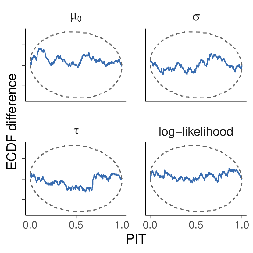
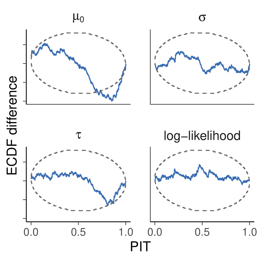
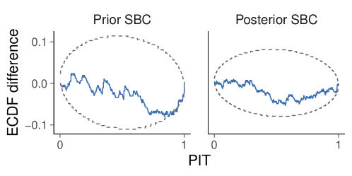
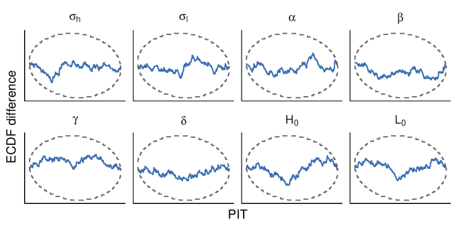
To assess the calibration of the inference, we inspect the uniformity of the PIT values of the joint log-likelihood, and of the parameters , , shared between the groups. We employ the graphical uniformity test introduced by Säilynoja et al., (2022), see e.g., Figure 3. The test shows 95% simultaneous central confidence bands for the empirical cumulative distribution function (ECDF) of the discrete PIT values under the assumption of calibration. The PIT values for a given quantity are obtained by transforming the quantity with respect to the corresponding posterior draws, see Figure 2. That is, for the population parameters, the prior draw is transformed with respect to the posterior draws. For the joint log-likelihood, we compare the log-likelihood of the sample, when evaluated with the known true parameter values, against the joint log-likelihood evaluated with the parameter posterior draws.
For prior SBC, Figure 3 shows no noticeable calibration issues in the inference with either parameterization. This would indicate to the modeller that everything is fine with either of these model implementations.
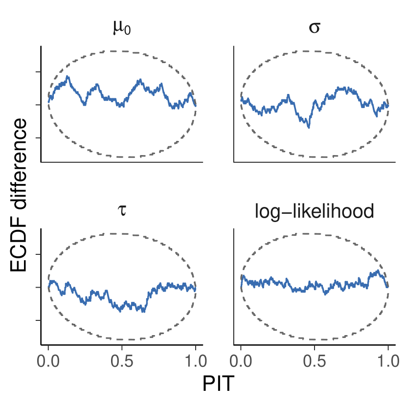
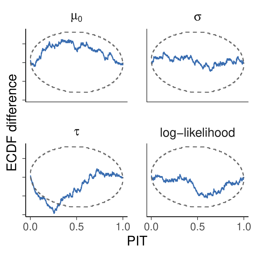
Next, we assess the calibration via posterior SBC by conditioning on the dataset with large and small . This corresponds to the weak population prior and strong likelihood case, implying a funnel shaped posterior with the non-centered parameterization. Running 500 iterations of posterior SBC reveals a very different story for the calibration of the two parameterizations. As shown in Figure 4, the centered parameterization shows excellent calibration, but the non-centered parameterization has calibration issues when evaluating the population level parameters and
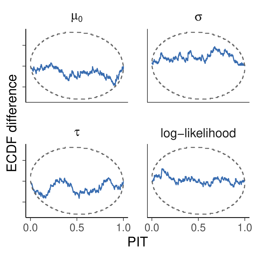
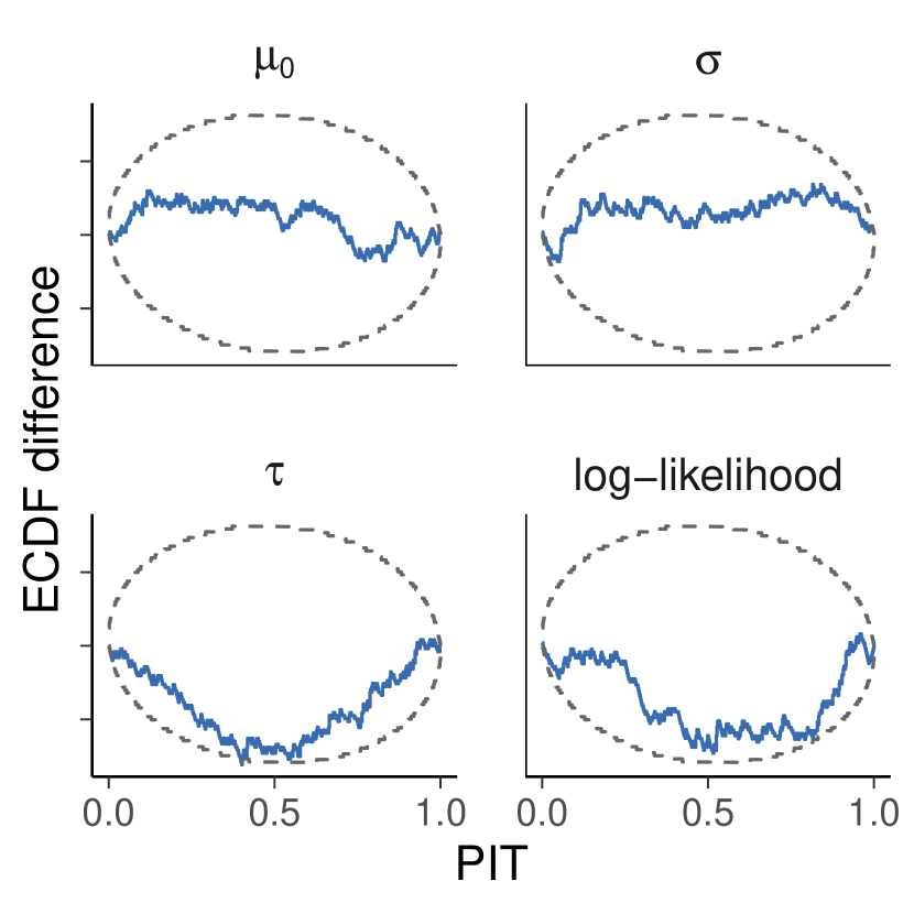
With the second dataset, generated with small and large corresponding to a case of strong population prior and weak likelihood, implying funnel shape for the posterior of the parameters in the model with centered parameterization. The posterior exhibits highly varying curvature, making it hard to explore for the inference algorithm. When we run posterior SBC conditional on this data, the presence of calibration issues with the centered parameterization of the model is confirmed. Figure 5 shows the calibration assessment of posterior SBC, revealing the clear calibration issues with the centered parameterization, but also showing possible overestimation of in the inference run with the non-centered parameterization. If we would like to inspect this effect more closely, we could run posterior SBC with more iterations to increase the sensitivity of the calibration checking.
To conclude, in this example, we showcased a model where prior SBC indicates no calibration issues with either of the candidate model implementations. In contrast, with posterior SBC, we observed that for both of the inspected datasets better calibration is achieved with one of the parameterizations, conditional on a given observed dataset.
In the presented cases, Stan interface conducted automated inference diagnostics, producing warnings for one or both of the parameterizations. In prior SBC both of the model parameterizations faced a considerable number of iterations with high values (Vehtari et al.,, 2021), implying bad mixing of the MCMC chains. Additionally, of the iterations of the centered parameterization model had one or more divergent transitions, implying possibly biased posterior inference. In posterior SBC, the first dataset with strong likelihood produced warnings for the non-centered parameterization, and the second dataset with weak likelihood was problematic for the centered parameterization. These warnings align with our findings with SBC by also indicating the inference problems. This is plausible since the issues are caused by the challenging posterior geometry. However, good diagnostics are not necessarily available for new inference methods, or as shown in Section 3.3, when the model complexity grows, the inference issues might be more subtle, but still have a strong impact on the posterior estimates and calibration.
3.2 Lotka-Volterra model – focusing computational efforts
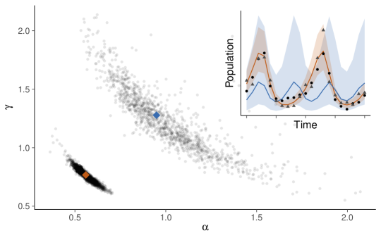
In this case study, we highlight how weakly informative priors can cause prior SBC to face computational issues, and how posterior SBC may provide substantial speed-ups for the calibration checking process. Additionally, we demonstrate a case where prior SBC indicates potential calibration issues for the model. However, these issues are not present in the parameter space explored by posterior SBC. Below, we show the results of performing both prior and posterior SBC for an inference task involving the Lotka-Volterra predator-prey model. We compare the findings of the calibration checking approaches, as well as the required computational efforts.
Setup
The Lotka-Volterra predator-prey model consist of a system of first order non-linear differential equations, and describes the population dynamics of an interacting pair of species, a predator and its prey. Here we model the number of snowshoe hare and Canada lynx pelts collected by the Hudson Bay Company between years 1900 and 1920 (Odum and Barrett,, 2005). The expectations of the number of pelts collected are modelled as the solutions to the Lotka-Volterra equations,
| (4) | ||||
| (5) |
where and are the populations of hares and lynxes respectively, is the rate at which the hare population would grow if no lynxes were present, and conversely is the death rate of lynxes without hares to hunt. The parameters and characterize the effect that the interaction between the species has on their populations – some hares get eaten, and the lynx population may grow. The signs in the equation system are chosen so that we expect each parameter to be positive.
We add an error term to model the measurement noise and the variation unexplained by the deterministic differential equation model. For both populations, the number of collected pelts is assumed to be log-normally distributed as
| (6) | |||
| (7) |
where and are the recorded numbers of pelts collected, and the latent true (trappable) populations of the species at that time, and and the error terms related to the species. All of these parameters are constrained to be positive. We don’t have strong intuition on the interactions between the Lotka-Volterra model parameters, so we assign them the following independent priors, used for example in the case study of Carpenter, (2018),
| (8) | ||||
| (9) |
These priors are set with the aim to inform on the magnitude of the parameters and to keep the year-to-year variation of the populations from being too extreme. For both of the measurement error terms, we set a weakly informative log-normal prior:
| (10) |
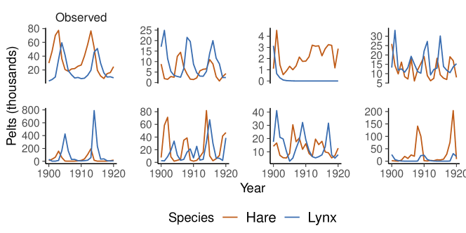
Figure 6 shows some prior predictive draws from the model together with the historical observations that will later use for posterior SBC. We describe these prior predictions more below, when discussing the results of the case study.
We implement the models using Stan and use NUTS for the posterior inference. This time, we initialize the Markov chains using the Pathfinder variational inference method (Zhang et al.,, 2022), which allows us to quickly obtain approximate draws close to the typical set of the posterior. This initialization step was added to the inference as the resulting posteriors are often multi-modal with a narrow high-probability mode corresponding to lower measurement error and a more informative likelihood for the ODE parameters, and a wider low-probability mode corresponding to high measurement error and low information on the ODE model parameters. With random initialization, some of the Markov-chains are prone to getting stuck on the low-probability mode, but Pathfinder can quickly find both modes and generate draws from the high-probability mode to be used as initial values for the Markov chains. Figure 7 shows an example of this posterior multimodality.
Results
We set out to run 250 iterations of both prior SBC and posterior SBC, but could extend posterior SBC to 500 iterations, as the runtime per iteration was over five times faster for posterior SBC. The process of running 250 iterations of prior SBC took 6.5 hours when using parallel processing for sampling the individual MCMC chains, but sequential model fitting. Conversely, after using 10 seconds to run the initial posterior inference on the historical pelt dataset published by Mahaffy, (2010), running 500 iterations of posterior SBC took only 2.5 hours.
In prior SBC, we observe some prior predictive draws resulting in posterior inference with severe convergence issues. When investigating the calibration of the inference, we look at the PIT-ECDF of the joint log-likelihood in Figure 8. There, we see some potential calibration issues manifesting as fewer than expected PIT values between 0.5 and 1. The calibration assessment for the individual parameters can be found in the appendix, but shows no calibration issues for the individual parameters before corrections for multiple testing.
Posterior SBC, in turn, indicates good calibration for the observed historical data. A graphical assessment of the uniformity of the PIT joint log-likelihood values is shown in Figure 8. The faster inference during the posterior SBC allowed us to iterate on the model and experiment on using Pathfinder for initializing the MCMC chains in the more desirable posterior mode. More details are shown in Appendix A.1.
To conclude, we have demonstrated a case, where the calibration issues indicated by prior SBC are not present once we condition on an observed dataset. Moreover, due to the problematic inference in prior SBC, posterior SBC turns out to be computationally less demanding and thus allows us to obtain more power on the calibration assessment while using a lower computational budget.
The observed inference problems during prior SBC are due to the independent weakly informative priors assigning a considerable prior probability to problematic parameter combinations, that are no longer plausible under the observation. Furthermore, when we inspect the prior predictive samples in Figure 6, we observe multiple samples that do not align with our expectations on the periodic nature of the data. We could try to improve the prior, but if the computation already works for the posterior it is not needed.
3.3 Posterior SBC in amortized Bayesian inference
In this case study, we show how posterior SBC can serve as a powerful diagnostic for amortized Bayesian inference workflows. Amortized Bayesian inference (see Zammit-Mangion et al.,, 2024, for an overview) constitutes a new wave of Bayesian inference methods, where neural networks learn a direct surrogate for the posterior distribution. Normalizing flows (Papamakarios et al.,, 2021) are arguably the most prominent neural density estimator for amortized inference, but other architectures have recently been explored as well, such as score-based diffusion models (Geffner et al.,, 2023; Sharrock et al.,, 2024), flow matching (Dax et al.,, 2023), and consistency models (Schmitt et al., 2023b, ).
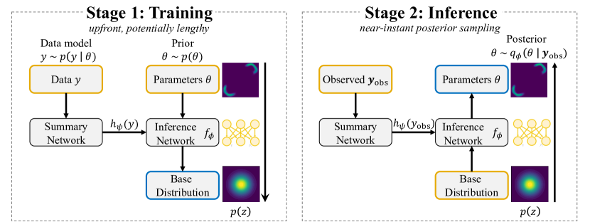
Amortized inference consists of two stages: (1) A training stage, where a generative neural network learns to distill relevant information from the probabilistic model based on synthetic data from the joint model; and (2) the inference stage, where the trained neural networks approximate the posterior distribution for an arbitrary new dataset . Amortized inference casts fitting a probabilistic model as a neural network prediction task, which typically takes well under a second. This achieves near-instant approximate posterior sampling and even direct posterior density evaluations for arbitrary parameter values .
In an effort to align amortized inference with the needs of common probabilistic modeling settings, there are two crucial extensions to the standard approach described above. First, in Bayesian inference, the data can be replaced by sufficient summary statistics without altering the posterior: . In amortized inference, neural networks are employed to learn embeddings of the data in tandem with the posterior approximator (Radev et al., 2020a, ; Radev et al., 2020b, ; Chen et al.,, 2021; Chan et al.,, 2018; Huang et al.,, 2023; Schmitt et al., 2023a, ). These summary networks are parameterized by learnable neural network weights and learn a fixed-length representation of the data which is approximately sufficient for posterior inference (not necessarily for reconstructing the data). Second, datasets can come with a varying number of observations . While the summary network learns to compress datasets of varying length to a fixed-length vector , the Bayesian posterior is influenced by the number of observations (e.g., as described by contraction). Hence, the neural network needs to be informed about the number of observations in the raw dataset, and we need to cover datasets with varying numbers of observations in the neural network training stage. Accordingly, we draw the number of observations in each simulated dataset from a distribution and condition the generative neural network on in addition to the learned summary statistics . In summary, the forward simulation process is formalized as
| (11) |
The resulting neural network training for a conditional normalizing flow with learned summary statistics and the number of observations as additional conditioning variable minimizes the maximum likelihood objective,
| (12) |
where the expectation is taken over the joint distribution .
However, there is no free lunch, and state-of-the-art amortized inference methods still lack the gold-standard guarantees from established algorithms like MCMC. The two most pressing issues of amortized neural posterior estimators are (1) the increased number of design choices from neural network architectures and training hyperparameters; and (2) the lack of performance guarantees under domain shifts between the simulated training data and the real data , for example resulting from model misspecification. As a consequence, there is a need for strong diagnostics to gauge the trustworthiness of amortized neural posterior approximators. In the context of non-amortized MCMC, one bottleneck of simulation-based calibration (both prior and posterior SBC) is the associated computational burden from repeated model re-fits on new simulated datasets. Yet, an amortized approximator can sample the required approximate posterior draws for new datasets in near-instant time, which reduces the runtime for SBC to only a few seconds. Therefore, posterior SBC naturally lends itself to amortized inference due to (1) the particular need for strong diagnostics; and (2) the stunningly quick runtime with an amortized approximator.
Setup
To improve our understanding of human cognition, researchers employ increasingly sophisticated statistical models to explore the neurological connections between cognitive processes and physical phenomena. From a mathematical perspective, human decision-making can be represented by a stochastic evidence accumulation process, specifically through a drift-diffusion model (DDM; Voss et al.,, 2004; Ratcliff and McKoon,, 2008). The DDM assumes that human decision-making is based on sequential integration of evidence over time until it reaches a threshold. The model is parameterized by an individual’s cognitive parameters (e.g., information uptake speed and decision thresholds). In its general form, a DDM is mathematically described by a differential equation,
| (13) |
where is the drift rate and controls the stochastic variance of the Wiener process . Simulation programs use a discretized version of the process,
| (14) |
where is Gaussian noise and controls the time resolution (5 milliseconds in our data model). The DDM is additionally parameterized by a decision threshold , an evidence starting point to represent biases, and a non-decision time to account for motor reaction times. We refer to Appendix A.2 for more details.
In a line of applied work, neurological research has identified neural markers that are associated with decision-making processes. In a recent paper, Ghaderi-Kangavari et al., (2023) propose a set of multiple statistical models that integrate both the cognitive drift-diffusion model and a compressed representation of neural measurements, as found in EEG or fMRI data. Such integrative models, which combine neural processes at the level of single experimental trials, represent the current state-of-the-art in cognitive modeling research. This case study implements two probabilistic models and , which correspond tomodels #2 and #6 from Ghaderi-Kangavari et al., (2023). We use deep neural networks to fit an amortized posterior approximator for each model. Detailed specifications of models and neural networks can be found in Appendix A.2. We showcase how posterior SBC can yield important information to compare the neural approximations of the candidate models conditional on two real datasets from another study (Georgie et al.,, 2018).
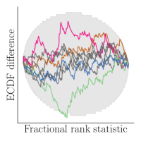
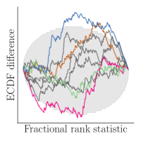
| Prior SBC, | Prior SBC, | Posterior SBC | Posterior SBC |
|---|---|---|---|
 |
 |
 |
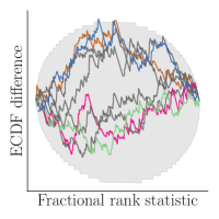 |
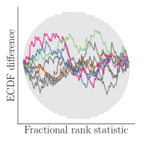
| Prior SBC, | Prior SBC, | Posterior SBC | Posterior SBC |
|---|---|---|---|
 |
 |
 |
 |
Results
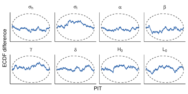
In the following, we summarize the main results of the case study and refer to Appendix A for additional details. In neural amortized inference, we must check the inference validity for different numbers of observations because the latter is passed as a conditioning variable to the inference network . To this end, we confirm that amortized inference on synthetic datasets simulated from the joint model can recover the ground-truth values of the model parameters that are identifiable for both and (see Appendix A). Further, we can confirm that prior SBC checking for datasets with as well as yields satisfactory results (see Figure 10). However, this conclusion drastically changes when we perform SBC checking conditional on the real datasets and . As shown in 10(a), posterior SBC indicates minor data-conditional calibration issues of model for the first observed dataset while calibration conditional on the second observed dataset is within the acceptance band. The second model , however, shows pathologically bad calibration of the mean visual encoding latency conditional on either observed dataset (see 10(b)). As a consequence, model might be refined according to the iterative Bayesian workflow (Gelman et al.,, 2020; Schad et al.,, 2020) with a particular focus on the mean visual encoding latency parameter . In this case study, posterior SBC could flag calibration issues of an amortized approximator that were not detectable with prior SBC, which illustrates its potential as a default data-conditional diagnostic in amortized Bayesian workflows (Radev et al.,, 2023; Schmitt et al.,, 2024).
4 Discussion
Prior SBC and posterior SBC have different roles in the Bayesian workflow. Posterior SBC can be used to diagnose whether the used inference algorithm is sampling faithfully from the posterior and the augmented posteriors, which are close to the original posterior. If there is a worry that the augmented posterior is too different from the original posterior having double data size, for it is possible to use part of the data for the first posterior and make the augmented data size to be more similar with the original data size.
Passing posterior SBC checking is a necessary but not sufficient condition to trust the posterior inference in the same way as most convergence diagnostics given finite computation time. If the common MCMC diagnostics like divergences and indicate big problems, it is good to first investigate the possible reasons before spending computation time for posterior SBC.
Posterior SBC is specifically useful when the usual diagnostics may have missed something, when the usual diagnostics may have false positive warnings, when using new algorithm implementations that are not yet trusted, or when using new inference algorithms which do not yet have faster diagnostics. Posterior SBC seems to be specifically useful for amortized inference, as the computational cost for repeated inference is low.
Data and code availability
Code to reproduce all experiments is available in the public repository at https://github.com/TeemuSailynoja/posterior-sbc.
Acknowledgments
We acknowledge the computational resources provided by the Aalto Science-IT project via the Triton compute cluster. TS and AV acknowledge the support by the Research Council of Finland Flagship programme: Finnish Center for Artificial Intelligence, and Research Council of Finland project (340721). MS and PCB acknowledge support of Cyber Valley Project CyVy-RF- 2021-16 and the DFG under Germany’s Excellence Strategy – EXC-2075 - 390740016 (the Stuttgart Cluster of Excellence SimTech). MS acknowledges the European Union’s Horizon 2020 research and innovation programme under grant agreements No 951847 (ELISE) and No 101070617 (ELSA), and the ELLIS PhD program. PCB acknowledges support of the DFG Collaborative Research Center 391 (Spatio-Temporal Statistics for the Transition of Energy and Transport) – 520388526.
References
- Carpenter, (2018) Carpenter, B. (2018). Predator-prey population dynamics: the Lotka-Volterra model in Stan. Technical report, Columbia University.
- Chan et al., (2018) Chan, J., Perrone, V., Spence, J., Jenkins, P., Mathieson, S., and Song, Y. (2018). A likelihood-free inference framework for population genetic data using exchangeable neural networks. Neural Information Processing Systems, 31.
- Chen et al., (2021) Chen, Y., Zhang, D., Gutmann, M. U., Courville, A., and Zhu, Z. (2021). Neural approximate sufficient statistics for implicit models. In International Conference on Learning Representations.
- Cook et al., (2006) Cook, S. R., Gelman, A., and Rubin, D. B. (2006). Validation of software for Bayesian models using posterior quantiles. Journal of Computational and Graphical Statistics, 15(3):675–692.
- Dax et al., (2023) Dax, M., Wildberger, J., Buchholz, S., Green, S. R., Macke, J. H., and Schölkopf, B. (2023). Flow matching for scalable simulation-based inference. In Neural Information Processing Systems.
- Drugowitsch et al., (2012) Drugowitsch, J., Moreno-Bote, R., Churchland, A. K., Shadlen, M. N., and Pouget, A. (2012). The cost of accumulating evidence in perceptual decision making. The Journal of Neuroscience, 32(11):3612–3628.
- Geffner et al., (2023) Geffner, T., Papamakarios, G., and Mnih, A. (2023). Compositional score modeling for simulation-based inference. In Krause, A., Brunskill, E., Cho, K., Engelhardt, B., Sabato, S., and Scarlett, J., editors, Proceedings of the 40th International Conference on Machine Learning, volume 202 of Proceedings of Machine Learning Research, pages 11098–11116. PMLR.
- Gelman, (2017) Gelman, A. (2017). Correction to Cook, Gelman, and Rubin (2006). Journal of Computational and Graphical Statistics, 26(4):940–940.
- Gelman et al., (2017) Gelman, A., Simpson, D., and Betancourt, M. (2017). The prior can often only be understood in the context of the likelihood. Entropy, 19(10):555.
- Gelman et al., (2020) Gelman, A., Vehtari, A., Simpson, D., Margossian, C. C., Carpenter, B., Yao, Y., Kennedy, L., Gabry, J., Bürkner, P.-C., and Modrák, M. (2020). Bayesian workflow. arXiv:2011.01808.
- Georgie et al., (2018) Georgie, Y. K., Porcaro, C., Mayhew, S. D., Bagshaw, A. P., and Ostwald, D. (2018). A perceptual decision making EEG/fMRI data set. bioRxiv 253047.
- Ghaderi-Kangavari et al., (2023) Ghaderi-Kangavari, A., Rad, J. A., and Nunez, M. D. (2023). A general integrative neurocognitive modeling framework to jointly describe EEG and decision-making on single trials. Computational Brain and Behavior, 6:317–376.
- Hawkins et al., (2015) Hawkins, G. E., Forstmann, B. U., Wagenmakers, E.-J., Ratcliff, R., and Brown, S. D. (2015). Revisiting the evidence for collapsing boundaries and urgency signals in perceptual decision-making. The Journal of Neuroscience, 35(6):2476–2484.
- Hoffman and Gelman, (2014) Hoffman, M. D. and Gelman, A. (2014). The No-U-turn sampler: adaptively setting path lengths in Hamiltonian Monte Carlo. Journal of Machine Learning Research, 15(1):1593–1623.
- Huang et al., (2023) Huang, D., Bharti, A., Souza, A. H., Acerbi, L., and Kaski, S. (2023). Learning robust statistics for simulation-based inference under model misspecification. In Neural Information Processing Systems.
- Mahaffy, (2010) Mahaffy, J. M. (2010). Math 636 - Mathematical Modeling Fall Semester, 2010 Lotka-Volterra Models. http://jmahaffy.sdsu.edu/courses/f09/math636/lectures/lotka/qualde2.html.
- Modrák et al., (2023) Modrák, M., Moon, A. H., Kim, S., Bürkner, P., Huurre, N., Faltejsková, K., Gelman, A., and Vehtari, A. (2023). Simulation-based calibration checking for Bayesian computation: The choice of test quantities shapes sensitivity. Bayesian Analysis.
- Odum and Barrett, (2005) Odum, E. P. and Barrett, G. W. (2005). Fundamentals of ecology. Thomson Brooks/Cole, Belmont, CA, 5th edition.
- Papamakarios et al., (2021) Papamakarios, G., Nalisnick, E., Rezende, D. J., Mohamed, S., and Lakshminarayanan, B. (2021). Normalizing flows for probabilistic modeling and inference. Journal of Machine Learning Research, 22(1).
- Papaspiliopoulos et al., (2007) Papaspiliopoulos, O., Roberts, G. O., and Sköld, M. (2007). A general framework for the parametrization of hierarchical models. Statistical Science, 22(1).
- (21) Radev, S. T., Mertens, U. K., Voss, A., Ardizzone, L., and Köthe, U. (2020a). BayesFlow: Learning complex stochastic models with invertible neural networks. IEEE Transactions on Neural Networks and Learning Systems.
- (22) Radev, S. T., Mertens, U. K., Voss, A., and Köthe, U. (2020b). Towards end-to-end likelihood-free inference with convolutional neural networks. British Journal of Mathematical and Statistical Psychology, 73(1):23–43.
- Radev et al., (2023) Radev, S. T., Schmitt, M., Schumacher, L., Elsemüller, L., Pratz, V., Schälte, Y., Köthe, U., and Bürkner, P.-C. (2023). BayesFlow: Amortized Bayesian workflows with neural networks. Journal of Open Source Software, 8(89):5702.
- Ratcliff and McKoon, (2008) Ratcliff, R. and McKoon, G. (2008). The diffusion decision model: Theory and data for two-choice decision tasks. Neural Computation, 20(4):873–922.
- Ratcliff et al., (2016) Ratcliff, R., Smith, P. L., Brown, S. D., and McKoon, G. (2016). Diffusion decision model: Current issues and history. Trends in Cognitive Sciences, 20(4):260–281.
- Schad et al., (2020) Schad, D. J., Betancourt, M., and Vasishth, S. (2020). Toward a principled Bayesian workflow in cognitive science. arXiv:1904.12765.
- (27) Schmitt, M., Bürkner, P.-C., Köthe, U., and Radev, S. T. (2023a). Detecting Model Misspecification in Amortized Bayesian Inference with Neural Networks. In 45th German Conference on Pattern Recognition (GCPR).
- Schmitt et al., (2024) Schmitt, M., Li, C., Vehtari, A., Acerbi, L., Bürkner, P.-C., and Radev, S. T. (2024). Amortized Bayesian workflow (extended abstract). In NeurIPS Workshop on Bayesian Decision-Making and Uncertainty.
- (29) Schmitt, M., Pratz, V., Köthe, U., Bürkner, P.-C., and Radev, S. T. (2023b). Consistency models for scalable and fast simulation-based inference. arXiv:2312.05440.
- Sharrock et al., (2024) Sharrock, L., Simons, J., Liu, S., and Beaumont, M. (2024). Sequential neural score estimation: Likelihood-free inference with conditional score based diffusion models. In Salakhutdinov, R., Kolter, Z., Heller, K., Weller, A., Oliver, N., Scarlett, J., and Berkenkamp, F., editors, Proceedings of the 41st International Conference on Machine Learning, volume 235 of Proceedings of Machine Learning Research, pages 44565–44602. PMLR.
- Stan Development Team, (2023) Stan Development Team (2023). Stan Users Guide and Reference Manual. https://mc-stan.org.
- Säilynoja et al., (2022) Säilynoja, T., Bürkner, P.-C., and Vehtari, A. (2022). Graphical test for discrete uniformity and its applications in goodness-of-fit evaluation and multiple sample comparison. Statistics and Computing, 32(2):32.
- Talts et al., (2020) Talts, S., Betancourt, M., Simpson, D., Vehtari, A., and Gelman, A. (2020). Validating Bayesian inference algorithms with simulation-based calibration. arXiv:1804.06788.
- Vehtari et al., (2021) Vehtari, A., Gelman, A., Simpson, D., Carpenter, B., and Bürkner, P.-C. (2021). Rank-normalization, folding, and localization: An improved for assessing convergence of MCMC (with discussion). Bayesian Analysis, 16(2):667–718.
- Voss et al., (2004) Voss, A., Rothermund, K., and Voss, J. (2004). Interpreting the parameters of the diffusion model: An empirical validation. Memory & Cognition, 32(7):1206–1220.
- Zaheer et al., (2017) Zaheer, M., Kottur, S., Ravanbhakhsh, S., Póczos, B., Salakhutdinov, R., and Smola, A. J. (2017). Deep sets. In Neural Information Processing Systems, page 3394–3404.
- Zammit-Mangion et al., (2024) Zammit-Mangion, A., Sainsbury-Dale, M., and Huser, R. (2024). Neural methods for amortised inference. arXiv:2404.12484.
- Zhang et al., (2022) Zhang, L., Carpenter, B., Gelman, A., and Vehtari, A. (2022). Pathfinder: Parallel quasi-Newton variational inference. Journal of Machine Learning Research, 23(306):1–49.
Appendix A Case studies: Details and additional results
This supplement provides details and additional results for the case studies of the main paper. The source code for reproducing these case studies is available at https://github.com/TeemuSailynoja/posterior-sbc.
A.1 Case study 2: Lotka-Volterra model
Below, we present calibration assessments, as well as parameter recovery results for the individual model parameters for both prior and posterior SBC of the Lotka-Volterra model implementation.
In Figure 11 we display the graphical calibration assessment of the individual parameters obtained with prior SBC for the Lotka-Volterra model. Even without correction for multiple comparison, the inference of the parameter posteriors looks well calibrated. In the parameter recovery plots for prior SBC, displayed in Figure 12, we see no systematic biases, but there are some cases where the posterior is very far from the ground truth. As discussed earlier in Section 3.2, these outliers are likely due to the posterior often having distinct modes corresponding to high and low measurement error. This leads to a high probability of one or more of the MCMC chains not properly exploring the full posterior.
Figure 13 and Figure 14 show the calibration assessment and recovery of the individual parameters once we condition the inference on the historical observations. Again, we observe no calibration issues. The parameter recovery also exhibits no outliers similar to those observed in prior SBC.
A.2 Case study 3: Posterior SBC checking in amortized Bayesian inference
In the following, we detail the full neural network settings as well as model specifications in case study 3, and present additional results concerning the parameter recovery of the amortized approximators.
Training setup and neural network settings
The prior distribution on the number of observations in the synthetic training datasets is an integer-valued uniform distribution . The summary network is a DeepSet (Zaheer et al.,, 2017) with mean-pooling, which combines equivariant and invariant neural network layers to extract a 32-dimensional summary vector from each dataset , where as specified above. The inference network is an affine coupling flow with 6 coupling layers. We train the neural network tandem for a total of 300 epochs with a batch size of 64, 1000 iterations per epochs, and determine the learning rate based on a cosine decay schedule with initial value of .
Model 1
The first probabilistic model corresponds to “model 2” in Ghaderi-Kangavari et al., (2023). It has the following data model,
| (15) | ||||
where denotes a Wiener drift-diffusion model with threshold , non-decision time , average drift rate , and initial bias . We use the following prior distributions from Ghaderi-Kangavari et al., (2023):
| (16) | ||||||||
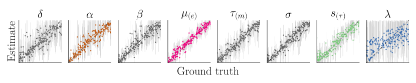
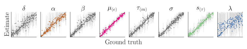
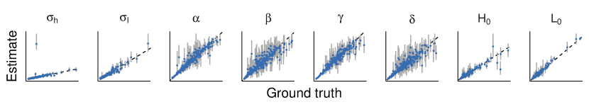
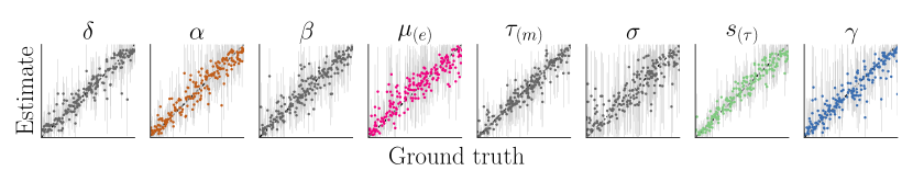
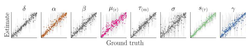
Figure 15 shows the parameter recovery of the amortized approximator across a range of settings. We observe that most parameters can be recovered with sufficiently high accuracy given the number of available observations in each dataset (see 15(a)). Further, the epistemic uncertainty in the parameter estimates shrinks as the number of observations grows (see 15(b)). Finally, errors in the posterior estimates propagate into the parameter recovery based on simulated data from the approximate posterior predictive distribution (see 15(c),15(d)). This evaluation follows the same principle as posterior SBC but reports the data-conditional parameter recovery rather than the data-conditional simulation-based calibration results. In summary, the patterns from the empirical parameter recovery match the results from (prior and posterior based) simulation-based calibration checking in Section 3.3.
Model 2
The second probabilistic model represents “model 6” by Ghaderi-Kangavari et al., (2023), which implements a drift-diffusion model with collapsing boundary (Drugowitsch et al.,, 2012; Hawkins et al.,, 2015; Ratcliff et al.,, 2016). The collapsing boundaries are formalized through a scaled Weibull cumulative distribution function,
| (17) | ||||
with upper threshold and lower threshold as a function of the time passed in the experiment. Again, we follow Ghaderi-Kangavari et al., (2023) and use the following prior distributions:
| (18) | ||||||||
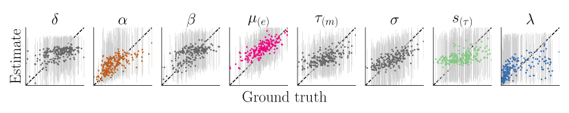
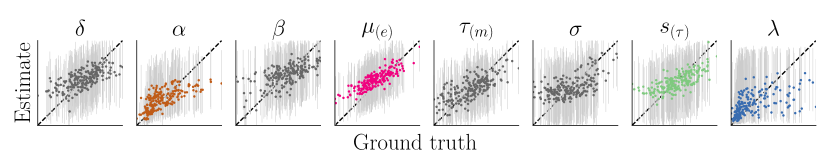
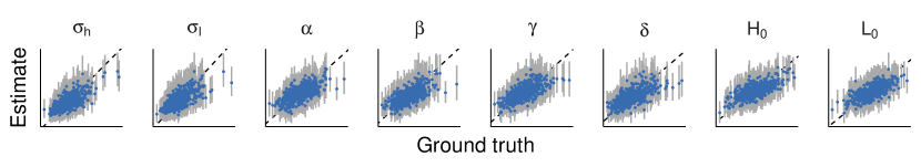
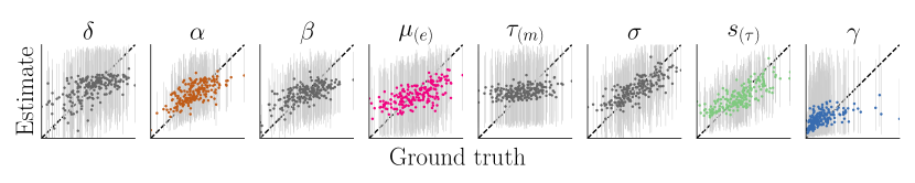
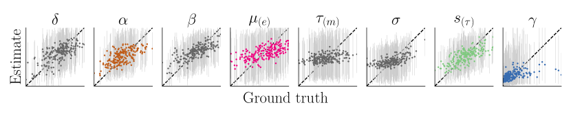
Paralleling the previous evaluation for model , Figure 16 reports the parameter recovery capabilities of the amortized approximator. Again, most parameters can be recovered with sufficiently high accuracy given the number of available observations in each dataset (see 16(a)), and the uncertainty shrinks when the datasets contain more observations (see 16(b)). The large epistemic uncertainty in the estimate of the boundary collapse parameter has previously been reported by Ghaderi-Kangavari et al., (2023). Furthermore, the parameter recovery patterns mirror the results from (prior and posterior based) simulation-based calibration checking in Section 3.3. Most notably, the previously reported data-conditional miscalibration in the parameter (10(b)) manifests in a biased data-conditional parameter recovery in 16(c),16(d).