Phase space analysis of CCDM cosmologies

Abstract

We perform a detailed investigation of the CCDM (creation of cold dark matter) cosmologies using the powerful techniques of qualitative analysis of dynamical systems. Considering a wide variety of the creation rates ranging from constant to dynamical, we examine the nature of critical points and their stability obtained from the individual scenario consisting of only cold dark matter, or cold dark matter plus a second fluid with constant equation of state. According to our analyses, these scenarios predict unstable dark matter dominated critical points, stable accelerating attractors dominated either by dark matter or the second fluid, scaling attractors in which both dark matter and the second fluid co-exist. Along with these critical points, these scenarios also indicate the possibility of decelerating attractors or decelerating scaling attractors in the future which are new results in this direction. These altogether suggest that CCDM cosmologies are viable alternatives to the mainstream cosmological models.

I Introduction

Accelerating expansion of the universe Riess et al. (1998); Perlmutter et al. (1999) is a major discovery of astrophysics and cosmology but the intrinsic mechanism behind this phenomenon is not clearly understood. Usually two well known approaches are considered in this regard: one is the introduction of some hypothetical dark energy (DE) fluid with sufficient negative pressure Caldwell et al. (1998); Caldwell (2002); Amendola (2000); Brax and Martin (2000); Astier (2001); Boyle et al. (2002); Kamenshchik et al. (2001); Linder (2003); Padmanabhan (2002); Debnath et al. (2004); Li (2004); Feng et al. (2006); Guo et al. (2005); Vikman (2005); Jassal et al. (2005); Gong (2004); Babichev et al. (2005); Chiba (2006); Cataldo et al. (2005); Zhang et al. (2006a, b); Zimdahl (2005); Scherrer (2006); Li et al. (2006); Guo et al. (2007); Cai (2007); Feng and Li (2009); Linder and Scherrer (2009); Li and Barrow (2009); Dutta et al. (2009); de Putter et al. (2010); Feng and Lu (2011); Ma and Zhang (2011); Solà and Gómez-Valent (2015); Das et al. (2018); Pan (2018); Pan et al. (2018); Yang et al. (2019); Almaraz et al. (2020); Yang et al. (2020); Saridakis (2020); Hernández-Almada et al. (2022); Yang et al. (2023); Kumar et al. (2023); Rezaei et al. (2024); Giarè et al. (2024) (also see Peebles and Ratra (2003); Copeland et al. (2006); Frieman et al. (2008); Li et al. (2011a, 2013a); Bamba et al. (2012a)) assuming that the Einstein’s General Relativity (GR) is the correct theory of gravity in the cosmological scales, and secondly, the modifications of the Einstein’s GR  Nojiri and Odintsov (2003); Nojiri et al. (2005); Nojiri and Odintsov (2005, 2006a); Amendola et al. (2007a); Li et al. (2007a); Brookfield et al. (2006); Nojiri and Odintsov (2007); Cognola et al. (2008); Amendola et al. (2007b); Li et al. (2007b); Tsujikawa (2008); Fay et al. (2007); Li et al. (2007c); de la Cruz-Dombriz et al. (2008); Brax et al. (2008); De Felice and Tsujikawa (2009); Thongkool et al. (2009); Zhou et al. (2009); Saridakis (2010); Miranda et al. (2009); Li et al. (2011b); Nojiri and Odintsov (2011); Li et al. (2011c); Paliathanasis et al. (2011); He et al. (2011); Geng et al. (2011); Li et al. (2011c); Harko et al. (2011); Li et al. (2013b); Chakraborty (2013); Bamba et al. (2012b); Odintsov and Sáez-Gómez (2013); He et al. (2013); Nojiri and Odintsov (2014); Thomas et al. (2015); Liu et al. (2016); Nunes et al. (2016); Paliathanasis et al. (2016); Nunes et al. (2017a); Kennedy et al. (2017); Nunes et al. (2017b); Hernández-Aguayo et al. (2019); Arnold et al. (2019); Atayde and Frusciante (2021); Lobato et al. (2021); Geng et al. (2022); Pan et al. (2021); dos Santos et al. (2022); Santos (2023); Davies et al. (2024) (known as Modified gravity, hereafter MG in short) can also explain this accelerating expansion (see the review articles in this direction Nojiri and Odintsov (2006b); De Felice and Tsujikawa (2010); Capozziello and De Laurentis (2011); Clifton et al. (2012); Koyama (2016); Cai et al. (2016); Nojiri et al. (2017); Akrami et al. (2021); Bahamonde et al. (2023)). Despite many efforts in constructing a variety of DE and MG models, an ultimate cosmological scenario consistent with all the observational datasets is still under the sea. Although the $\Lambda$-Cold Dark Matter ($\Lambda$CDM) model (constructed within the framework of GR) in which $\Lambda$ acts as DE, has been found to be quite successful with many astronomical probes, but the assumption of independent conservation of the cold dark matter (DM) and DE within this framework has no well founded explanation. It is well known that $\Lambda$CDM already faces many challenges, such as the cosmological constant problem Weinberg (1989), cosmic coincidence problem Zlatev and Steinhardt (1999), and cosmological tensions in recent times Di Valentino et al. (2021); Perivolaropoulos and Skara (2022); Abdalla et al. (2022). Thus, in principle, there is no reason to prefer any cosmological proposal over the other and new models are welcome provided they are found to be consistent with the observational data. An alternative scenario to both DE and MG approaches, namely, the theory of gravitationally induced adiabatic particle creation or matter creation was proposed in the literature Alcaniz and Lima (1999); Freaza et al. (2002); Steigman et al. (2009); Lima et al. (2010); Basilakos and Lima (2010); Lima et al. (2016) that can explain the late-time accelerating expansion of the universe. In fact, matter creation models can also explain the early inflationary era as well Abramo and Lima (1996); Gunzig et al. (1998) which is quite promising for a new cosmological scenario aiming to compete with existing cosmological proposals. The development of this theory started with a pioneering work by Prigogine, Geheniau, Gunzig and Nardone Prigogine et al. (1988) who established the link between the matter creation and the Einstein’s gravitational equations. In matter creation theory, the creation pressure caused by the produced particles plays the central role in driving the accelerating expansion of the universe. The creation pressure is directly linked with the rate of particle creation and the properties of the matter component from which the particles are created. As a result of which, without adding any hypothetical fluid or modifying the underlying gravitational theory, one can explain the accelerating phase of the universe. While looking at the large amount of works in the direction of DE (Refs. Caldwell et al. (1998); Caldwell (2002); Amendola (2000); Brax and Martin (2000); Astier (2001); Boyle et al. (2002); Kamenshchik et al. (2001); Linder (2003); Padmanabhan (2002); Debnath et al. (2004); Li (2004); Feng et al. (2006); Guo et al. (2005); Vikman (2005); Jassal et al. (2005); Gong (2004); Babichev et al. (2005); Chiba (2006); Cataldo et al. (2005); Zhang et al. (2006a, b); Zimdahl (2005); Scherrer (2006); Li et al. (2006); Guo et al. (2007); Cai (2007); Feng and Li (2009); Linder and Scherrer (2009); Li and Barrow (2009); Dutta et al. (2009); de Putter et al. (2010); Feng and Lu (2011); Ma and Zhang (2011); Solà and Gómez-Valent (2015); Das et al. (2018); Pan (2018); Pan et al. (2018); Yang et al. (2019); Almaraz et al. (2020); Yang et al. (2020); Saridakis (2020); Hernández-Almada et al. (2022); Yang et al. (2023); Kumar et al. (2023); Rezaei et al. (2024); Giarè et al. (2024)), and MG (Refs. Nojiri and Odintsov (2003); Nojiri et al. (2005); Nojiri and Odintsov (2005, 2006a); Amendola et al. (2007a); Li et al. (2007a); Brookfield et al. (2006); Nojiri and Odintsov (2007); Cognola et al. (2008); Amendola et al. (2007b); Li et al. (2007b); Tsujikawa (2008); Fay et al. (2007); Li et al. (2007c); de la Cruz-Dombriz et al. (2008); Brax et al. (2008); De Felice and Tsujikawa (2009); Thongkool et al. (2009); Zhou et al. (2009); Saridakis (2010); Miranda et al. (2009); Li et al. (2011b); Nojiri and Odintsov (2011); Li et al. (2011c); Paliathanasis et al. (2011); He et al. (2011); Geng et al. (2011); Li et al. (2011c); Harko et al. (2011); Li et al. (2013b); Chakraborty (2013); Bamba et al. (2012b); Odintsov and Sáez-Gómez (2013); He et al. (2013); Nojiri and Odintsov (2014); Thomas et al. (2015); Liu et al. (2016); Nunes et al. (2016); Paliathanasis et al. (2016); Nunes et al. (2017a); Kennedy et al. (2017); Nunes et al. (2017b); Hernández-Aguayo et al. (2019); Arnold et al. (2019); Atayde and Frusciante (2021); Lobato et al. (2021); Geng et al. (2022); Pan et al. (2021); dos Santos et al. (2022); Santos (2023); Davies et al. (2024)), it is fairly understood that even though the DE and MG models got massive popularity in the community compared to the models arising from the theory of particle creation, however, the matter creation models are equally compelling due to their simplicity and elegant nature, see also de Roany and Freitas Pacheco (2011); Lima et al. (2011); Jesus et al. (2011); Lima et al. (2012, 2014); Lima and Baranov (2014); Ramos et al. (2014); Fabris et al. (2014); Chakraborty et al. (2014); Baranov and Lima (2015); de Haro and Pan (2016); Pan et al. (2016); Paliathanasis et al. (2017); Biswas et al. (2017); Bhattacharya et al. (2018); Pan et al. (2019); Ivanov and Prodanov (2019a, b); Singh and Kaur (2019); Cárdenas et al. (2020a, b); Gohar and Salzano (2021); Kaur and Singh (2021); Cárdenas et al. (2021, 2022); Pinto et al. (2023); Trevisani and Lima (2023); Banerjee et al. (2024); Montani et al. (2024); Elizalde et al. (2024); Mandal and Biswas (2025); Cárdenas and Lepe (2025).

The heart of this theory is the matter creation rate $-$ the rate at which matter particles are created. For a given particle creation rate, one can in principle determine the dynamics of the universe. However, one of the limitations of matter creation theory is the unavailability of any fundamental theory which can evaluate the particle creation rate, hence, different choices for the particle creation rate are considered and the resulting cosmological scenario is tested with the observational data. This treatment is almost identical with the DE and MG gravity theories where a hypothetical fluid (in the context of GR) or an unknown modified gravity is considered at the beginning, and no fundamental principle is available so far that can correctly describe everything. Even though, for some specific phenomenological choices of $\Gamma$, see for instance Lima et al. (2010, 2016), one can mimic the $\Lambda$CDM-like cosmology, however, based on the ongoing debates in the scientific community Di Valentino et al. (2021); Perivolaropoulos and Skara (2022); Schöneberg et al. (2022); Abdalla et al. (2022); Kamionkowski and Riess (2023), $\Lambda$CDM is not the final destination of the universe, and most probably, new physics beyond $\Lambda$CDM is needed. Therefore, examining different matter creation rates is equally compelling and worth exploring given the fact that currently, the dynamics of the universe is still elusive.

Now under the assumption of any arbitrary matter creation rate, depending on its complexity, the gravitational field equations become complicated and finding the analytical solutions of the cosmological variables is not always possible. Even though one can always adopt the numerical techniques, however, in the present article, we have considered one of the potential tools in cosmology, namely, the qualitative analysis of dynamical systems which has been extensively used in the context of cosmological models. As far as we are concerned with the literature, the dynamical analysis of matter creating cosmologies did not get considerable attention to the community without any specific reason. In the present article, we have therefore performed a detailed phase space analysis of various matter creation scenarios using the techniques of dynamical analysis. According to our analysis, we found that the cosmological models endowed with matter creation are phenomenologically very rich and attractive.

The paper has been organized as follows. In section II, specifically in its first half, we describe the gravitational field equations for one fluid (section II.1) and two-fluid (section II.2) systems; and in the second half of this section, i.e. in section II.3 we present various matter creation models emerging from a general matter creation model. In section III we present the autonomous systems for the proposed matter creation models and examine the phase space analysis of the individual scenario. Finally, in section IV we conclude the present article with the main findings.

II Matter Creation Cosmology: One fluid and two-fluid systems

This section deals with the gravitational field equations of a matter creation cosmology. We consider two things to proceed with the matter creation cosmology. The first one is the validity of Einstein’s General Relativity in the cosmological scales and the second one is the homogeneous and isotropic universe which is well described by the spatially flat Friedmann-Lemaître-Robertson-Walker (FLRW) line element $ds^{2}=-{dt}^{2}+a^{2}(t)\left[dr^{2}+r^{2}\left(d\theta^{2}+\sin^{2}\theta d\phi^{2}\right)\right]$ in which $a(t)$ is the expansion scale factor of the universe. Now, let us assume a system having a volume $V$ attaining $N$ particles. In an open thermodynamical system, $N$ should be a function of time i.e. it changes with time. Thus, the conservation equation will transform to the form

$$N^{\mu}_{;\mu}\equiv\dot{n}+\Theta n=n\Gamma\Longleftrightarrow N^{\mu}_{,\mu}u^{\mu}=\Gamma N,$$ (1)

where $n=N/V$ is the particle density, $N^{\mu}=nu^{\mu}$ corresponds to the particle flow vector ($u^{\mu}$ represents the four velocity of the particle); ‘dot’ stands for the derivative with respect to the cosmic time $t$; $\Theta=u^{\mu}_{;\mu}$ is the expansion scalar of the fluid which in the FLRW universe becomes $3H$  ($H=\dot{a}(t)/a(t)$ is the Hubble rate of the FLRW universe), and $\Gamma$ is the rate of change of particle number. Here $\Gamma>0$ indicates the production of particles while $\Gamma<0$ indicates the reverse, that means particle annihilation. Now, using (1) in the Gibb’s equation Zimdahl (1996)

$$Tds=d\left(\frac{\rho}{n}\right)+pd\left(\frac{1}{n}\right),$$ (2)

where $T$ corresponds to the fluid temperature, $s$ indicates the specific entropy (or, the entropy per particle), $\rho$ denotes the total energy density and $p$ represents the total thermodynamic pressure, one appears with the following conservation equation

$$nT\dot{s}=\dot{\rho}+3H\left(1-\frac{\Gamma}{3H}\right)(\rho+p).$$ (3)

Considering an adiabatic (also known as isentropic) thermodynamic process where the rate of change of specific entropy vanishes (i.e. $\dot{s}=0$), eqn. (3) reduces to

$$\dot{\rho}+3H(\rho+p)=\Gamma(\rho+p),$$ (4)

which alternatively can be put as

$$\dot{\rho}+3H(\rho+p+p_{c})=0,$$ (5)

where the new term $p_{c}$ is termed as creation pressure due to the particle production and it takes the form

$$p_{c}=-\frac{\Gamma}{3H}(\rho+p).$$ (6)

This creation pressure has some interesting implications: if the fluid under consideration is a normal fluid, then for $\Gamma>0$, one can induce a negative creation pressure. As we shall explain in the following, this creation pressure can drive the accelerating phase of the universe and hence particle production scenario can be treated as a mirage of a DE. Now, concerning the matter sector, one can assume that i) the matter sector is comprised of only one fluid, for instance the pressure-less dark matter (DM), and this DM is endowed with gravitationally induced adiabatic matter creation Lima et al. (2010), or ii) the matter sector of the universe is comprised of $n$ arbitrary fluids and all of them can create gravitationally induced adiabatic matter particles Lima et al. (2016), or alternatively, ii) the matter sector is comprised of two mixed fluids where some fluids are able to create gravitationally induced adiabatic matter particles while the remaining fluids do not take part in the matter creation. Theoretically, all of the above possibilities are equally valid and appealing. In this work we shall consider two different matter creation cosmologies, namely, one fluid system in which the matter sector of the universe is comprised of only pressure-less DM sector blessed with gravitationally induced adiabatic matter creation, and secondly we shall consider a two-fluid system made of a pressure-less DM (responsible for the gravitationally induced adiabatic matter creation) and a general fluid with a barotropic equation of state which does not take part in the matter creation hypothesis; and in addition to that, both the fluids do not take part in an energy exchange mechanism, that means they are not interacting with each other. The introduction of the second fluid is motivated from the fact that the phase space structure of the matter creation cosmologies might be affected in presence of a second fluid which does not join in the matter creation process.

II.1 One fluid system

For the single fluid system, namely, pressure-less DM endowed with gravitationally induced adiabatic particle production, in the context of the FLRW background, the gravitational field equations become,

$$H^{2}=\frac{\kappa^{2}}{3}\;\rho_{\rm dm},$$ (7)

$$2\dot{H}+3H^{2}=-{\kappa}^{2}p_{c},$$ (8)

where $\kappa^{2}=8\pi G$ is the Einstein’s gravitational constant ($G$ is the Newton’s gravitational constant); $\rho_{\rm dm}$ is the energy density of the pressure-less DM, $p_{c}$ is the creation pressure which is related to the rate of particle production $\Gamma$ as Steigman et al. (2009); Lima et al. (2010); Basilakos and Lima (2010); de Haro and Pan (2016)

$$p_{c}=-\frac{\Gamma}{3H}\rho_{\rm dm}.$$ (9)

Here $\Gamma>0$ indicates the creation of particles and $\Gamma<0$ indicates the particle annihilation. It is interesting to note that the conservation equation of the pressure-less DM which follows from (7) and (8) is $\dot{\rho}_{\rm dm}+3H\left(1-\Gamma/3H\right)\rho_{\rm dm}=0$, is equivalent to the conservation equation of a non-cold DM fluid with variable equation of state of DM: $\dot{\rho}_{\rm dm}+3H(1+w_{\rm dm}(t))\rho_{\rm dm}$, where $w_{\rm dm}(t)=-\Gamma/3H$. Thus, the particle creation mechanism can be considered to be an equivalent prescription of the non-interacting cosmological scenario with a variable equation of state of the underlying fluid (here DM) responsible for this creation. Now, using (7), (8), and (9) one arrives at the acceleration equation

$$\frac{\ddot{a}}{a}=-\frac{\kappa^{2}}{6}\left(1-\frac{\Gamma}{H}\right)\rho_{\rm dm},$$ (10)

from which one can see that if $\Gamma<0$, then $\ddot{a}<0$ representing a decelerating phase of the universe. In order to realize an accelerating expansion of the universe, $\Gamma$ needs to satisfy $1-\Gamma/H<0$, which indicates that in an expanding universe (i.e. $H>0$), $\Gamma>H$. That means, the rate of particle creation should be positive.

II.2 Two-fluid system

In the two-fluid system, as already mentioned, one fluid is the pressure-less DM which is gifted with the gravitationally induced adiabatic matter creation and the second fluid does not take part in this matter creation process and both of them are independently conserved. The gravitational equations in the context of the FLRW universe become,

$$H^{2}=\frac{\kappa^{2}}{3}(\rho_{\rm dm}+\rho_{f}),$$ (11)

$$2\dot{H}+3H^{2}=-{\kappa}^{2}(p_{c}+p_{f}),$$ (12)

where $\rho_{f}$, $p_{f}$ are respectively the energy density and pressure of the second fluid; the creation pressure $p_{c}$ associated with the DM fluid is related to the particle creation or matter creation rate $\Gamma$ as in (9). The conservation equation of both the fluids become, $\dot{\rho}_{\rm dm}+3H(\rho_{\rm dm}+p_{c})=0$, and $\dot{\rho_{f}}+3H(1+w)\rho_{f}=0$, where $w=p_{f}/\rho_{f}$ is the barotropic equation-of-state of the second fluid and it could take any real number. Let us note that similar to the one-fluid system, the matter creating DM fluid is equivalent to a non-interacting DM fluid with variable equation of state. Now, concerning $w$, if it is a constant, then one can find the evolution of $\rho_{f}$ as, $\rho_{f}=\rho_{f0}(a/a_{0})^{-3(1+w)}$ where $\rho_{f0}$ is the present value of $\rho_{f}$ and $a_{0}$ is the scale factor at present time. If on the contrary, $w$ is dynamical, then depending on the nature of $w$, one can either solve $\rho_{f}$ analytically or numerically. However, the overall evolution of this matter creating cosmology depends on the matter creation rate $\Gamma$. In this work we focus on the constant $w$ in order to start with a simple scenario of matter creation cosmology. Finally, the accelerating equation in this case becomes,

$$\frac{\ddot{a}}{{a}}=-\frac{\kappa^{2}}{6}\left[\left(1-\frac{\Gamma}{H}\right)\rho_{\rm dm}+(1+3w)\rho_{f}\right].$$ (13)

From eqn. (13) one can clearly see that if we consider a normal fluid characterized by $w\geq 0$, then for $\Gamma<0$, we will never realize an accelerating expansion of the universe because in this case $\ddot{a}<0$, however, for $\Gamma>0$, it is possible to get $\ddot{a}>0$ provided the sum of the terms inside the third brace of the right hand side of eqn. (13) becomes negative. This can be obtained for some suitable choices of $\Gamma$. However, we further note that for $\Gamma<0$ it is not impossible to obtain the accelerating expansion of the universe, because in this case we need to allow $w<0$, that means particle annihilation alone cannot explain the accelerating expansion unless we add some hypothetical fluid from outside. This further strengthens the presence of a hypothetical fluid with negative pressure in the context of particle annihilation. While the focus of this work is not to consider some hypothetical fluid with negative pressure (i.e. $w<0$); we are mainly interested to investigate the effects of $\Gamma~(>0)$ on the accelerating expansion of the universe in presence of a normal fluid (i.e. $w\geq 0$). However, in the present article we shall allow both the non-negative and negative values of $w$ in order to compare the effects of $\Gamma$ on the resulting scenarios.

II.3 Models

Over the last couple of years, a variety of matter creation rates have been proposed in the literature Lima et al. (2011); Jesus et al. (2011); Lima et al. (2012, 2014); Lima and Baranov (2014); Chakraborty et al. (2014); Baranov and Lima (2015); de Haro and Pan (2016); Pan et al. (2016); Paliathanasis et al. (2017); Pan et al. (2019). In most of the cases, the choice of the matter creation rate $\Gamma$ is arbitrary since there is no fundamental guiding principle available yet in the literature, however, the resulting phenomenological scenarios become very appealing. A general choice of the matter creation follows

$$\Gamma=\sum_{j=1}^{\infty}\Gamma_{-j}(\mathcal{X})H^{-j}+\Gamma_{0}+\sum_{i=1}^{\infty}\Gamma_{i}(\mathcal{X})H^{i}$$ (14)

where $\mathcal{X}$ could be any cosmic variable, $\Gamma_{-j}(\mathcal{X})$’s, $\Gamma_{j}(\mathcal{X})$’s may not necessarily be dimensionless. We can only say that $\Gamma$ has the dimension of the Hubble rate. Thus, depending on the presence of $H^{i}$’s in the expression (14), the dimension of $\Gamma_{i}(\mathcal{X})$’s will be decided consequently. In order to proceed with the phase space analysis, a typical matter creation rate needs to be provided. Although one can start with a general matter creation rate from (14) which may involve the arbitrary powers of $H$, however, at the same time, the number of parameters will increase and understanding the phase space structure might be complicated. Thus, in the first half of the article we consider some simple choices of the matter creation rate as follows,

$$\Gamma=\Gamma_{0},$$ (15)

$$\Gamma=\Gamma_{0}H,\quad\Gamma=\Gamma_{0}H^{2},$$ (16)

$$\Gamma=\Gamma_{0}H^{-1},\quad\Gamma=\Gamma_{0}H^{-2},$$ (17)

and explain how different choices of the matter creation rate affects the phase space structure. In the second half of the article we consider various matter creation rates which are the linear combinations of $H$, $1/H$, $H^{2}$ and investigate the phase space analysis. We consider the following choices of the matter creation rate:

$$\Gamma=\Gamma_{0}+\Gamma_{1}H,$$ (18)

$$\Gamma=\Gamma_{0}+\Gamma_{3}H^{-1},$$ (19)

$$\Gamma=\Gamma_{0}+\Gamma_{2}H^{2},$$ (20)

$$\Gamma=\Gamma_{1}H+\Gamma_{2}H^{2},$$ (21)

$$\Gamma=\Gamma_{1}H+\Gamma_{3}H^{-1},$$ (22)

$$\Gamma=\Gamma_{0}+\Gamma_{1}H+\Gamma_{2}H^{2}.$$ (23)

With these matter creation models, one can cover a wide variety of models in the literature. As far as we are concerned with the literature, only a few models have been considered in the literature. Having these matter creation models, in the following we perform the phase space analysis of the individual model.

III Phase space Analysis

In order to proceed with the dynamical analysis, we introduce the following dimensionless variables

$$x=\frac{\kappa^{2}\rho_{\rm dm}}{3H^{2}},\quad\mbox{and}\quad z=\frac{H_{0}}{H_{0}+H},$$ (24)

where $H_{0}$ represents the present value of the Hubble rate. Now, using the dimensionless variables in (24), the gravitational equations for one fluid or two-fluid systems as described in section II can be converted into the autonomous systems. Considering the general matter creation rate $\Gamma$ in (14), the decelerating parameter, $q\equiv-1-\dot{H}/H^{2}$, for the one-fluid system reads

$$q=\frac{1}{2}\left(1-\frac{\Gamma}{H}\right),$$ (25)

and for two-fluid system in terms of the dimensionless variables in (24), takes the form

$$q=\frac{1}{2}\left[1+3w(1-x)-\frac{\Gamma}{H}x\right].$$ (26)

Therefore, given a particular model of $\Gamma$, one can determine the evolution of the deceleration parameter. In what follows, we present the autonomous systems for the proposed matter creation models and perform the stability of the critical points.

III.1 Model: $\Gamma=\Gamma_{0}$

In this section we shall discuss the effects of the constant particle creation rate $\Gamma=\Gamma_{0}$ considering a one fluid system and a two-fluid system.

III.1.1 One fluid system

From the first Friedmann eqn. (7), it is clear that the DM density parameter, $\Omega_{\rm dm}=\kappa^{2}\rho_{\rm dm}/3H^{2}$ always takes the value $1$. Thus, we are interested on the evolution of the $z$ variable. The dynamics of the matter creation model for $\Gamma=\Gamma_{0}$ can be described by the following one dimensional equation

$$z^{\prime}=\frac{3}{2}z\left(1-z-\frac{\alpha z}{3}\right),$$ (27)

where $\alpha=\Gamma_{0}/H_{0}>0$ is the dimensionless parameter and the prime denotes the derivative with respect to $N=\ln(a/a_{0})$. The decelerating parameter $q$ adopts the form $q=\frac{1}{2}\left(1-\frac{\alpha z}{1-z}\right)$ which at present time (i.e. at $z=\frac{1}{2}$) reduces to the form $q=\frac{1-\alpha}{2}$. Thus, at present time in order to realize an accelerating phase, the required condition is $\alpha>1$. The relevant critical points of the dynamical system (27) and their cosmological features are summarized in Table 1. In this case, we obtain only two critical points, namely, $A^{\prime}_{0},~A^{\prime}_{1}$ in which the first component corresponds to DM density parameter and second component represents the $z$ variable. Here $A^{\prime}_{0}$ is a DM dominated unstable point showing the decelerating phase, while $A^{\prime}_{1}$ is also a DM dominated stable critical point giving accelerating phase. The directions of the vector field involving in the system (27) are presented in the upper left plot of the Fig. 1 showing a transition of our universe from its past decelerating phase to the current accelerating one.

III.1.2 Two-fluid system

For the two-fluid system, considering the dimensionless variables, $x$, $z$ defined in eqn. (24), the constraint from the Friedmann equation (11) is, $\Omega_{\rm dm}+\Omega_{f}=1$ where $\Omega_{f}=\kappa^{2}\rho_{f}/(3H^{2})$. Now, using these dimensionless variables, one can write down the autonomous system as follows

$$x^{\prime}= x(1-x)\left(3w+\frac{\alpha z}{1-z}\right),$$ (28a)

$$z^{\prime}= \frac{3}{2}z(1-z)\left[1+w(1-x)-\frac{\alpha xz}{3(1-z)}\right],$$ (28b)

where $\alpha=\Gamma_{0}/H_{0}$ is a parameter which takes only positive values. For this model our physical region is a unit square and we define it as, $R_{1}=[0,1]^{2}$. The above autonomous system has a singularity at $z=1$, but we want access the phase space analysis of the points which correspond to $z=1$. So, we multiply the right hand sides of (28a), (28b) by the non-negative factor $(1-z)$ and regularize the autonomous system. Therefore, the reduced autonomous system can be read as:

$$x^{\prime}= x(1-x)\left(3w(1-z)+\alpha z\right),$$ (29a)

$$z^{\prime}= \frac{3}{2}z(1-z)\bigg{[}\bigg{(}1+w(1-x)\bigg{)}(1-z)-\frac{\alpha xz}{3}\bigg{]},$$ (29b)

From the above autonomous system, one can easily conclude that $x=0,~x=1,~z=0$ and $z=1$ are invariant manifolds which indicate that our physical region is positively invariant, i.e. if we take any orbit from $R_{1}$, it never leaves the domain. Here, the decelerating parameter defined in (26) is simplified to $q=\frac{1}{2}\left[1+3w(1-x)-\frac{\alpha xz}{1-z}\right]$. From this relation, one can quickly derive that in order to obtain the accelerating expansion at present time, i.e. at $z=1/2$, the viable orbits must satisfy the relation $(1-\alpha)x+(1+3w)(1-x)<0$.

Now, in order to understand the phase space dynamics of the autonomous system (29), we find the critical points and investigate their stability conditions. The critical points and their characteristics are summarized in Table 1. In this case, we find five discrete critical points ($A_{0}$, $A_{1}$, $A_{2}$, $A_{3}$, and $A_{4}$) and three critical lines ($A_{5}$, $A_{6}$ and $A_{7}$). Since the equation of state of the second fluid, $w$, is involved and as $w$ can take any value (either non-negative or negative), therefore, in order to understand how the nature of the second fluid affects the architecture of the phase space dynamics, we have paid special attention to the cases with $w\geq 0$ indicating the normal fluid and $w<0$ representing the hypothetical fluid. In the following we describe the qualitative features of the above dynamical system for different values of $w$.

		One fluid system
Critical point		Existence	Stability		$\Omega_{\rm dm}$	$q$	Acceleration
$A^{\prime}_{0}(1,0)$		Always	Always Unstable		1	$\frac{1}{2}$	No
$A^{\prime}_{1}\left(1,\frac{3}{3+\alpha}\right)$		$\alpha>0$	Always Stable		1	$-1$	Yes
		Two-fluid system
Critical point	Existence	Eigenvalue	Stability	$\Omega_{f}$	$\Omega_{\rm dm}$	$q$	Acceleration
$A_{0}(0,0)$	Always	$\left(3w,\frac{3}{2}(1+w)\right)$	Stable if $w<-1$;	1	0	$\frac{1}{2}(1+3w)$	$w<-\frac{1}{3}$
			Saddle if $-1<w<0$;
			Unstable if $w>0$
$A_{1}(1,0)$	Always	$\left(-3w,\frac{3}{2}\right)$	Saddle if $w>0$;	0	1	$\frac{1}{2}$	No
			Unstable if $w<0$
$A_{2}(0,1)$	Always	$(\alpha,0)$	Non-hyperbolic Saddle if $w>-1$	1	0	Undefined	Undetermined
			Unstable if $w<-1$
$A_{3}(1,1)$	Always	$\left(-\alpha,\frac{\alpha}{2}\right)$	Always Saddle	0	1	$-\infty$	Yes
$A_{4}\left(1,\frac{3}{3+\alpha}\right)$	$\alpha>0$	$\left(-\frac{3\alpha(1+w)}{3+\alpha},-\frac{3\alpha}{2(3+\alpha)}\right)$	Stable if $w>-1$	0	1	$-1$	Yes
			Saddle if $w<-1$
$A_{5}\left(0,z_{c}\right)$	$w=-1$	$\left((3+\alpha)z_{c}-3,0\right)$	Stable if $z_{c}<\frac{3}{3+\alpha}$;	$1$	$0$	$-1$	Yes
			Unstable if $z_{c}>\frac{3}{3+\alpha}$
$A_{6}\left(x_{c},\frac{3}{3+\alpha}\right)$	$w=-1$	$\left(0,-\frac{3\alpha x_{c}}{2(3+\alpha)}\right)$	Stable	$1-x_{c}$	$x_{c}$	$-1$	Yes
$A_{7}\left(x_{c},0\right)$	$w=0$	$\left(0,\frac{3}{2}\right)$	Unstable	$1-x_{c}$	$x_{c}$	$\frac{1}{2}$	No

Table 1: Summary of the critical points, their existence, stability and the values of the cosmological parameters at those points for the dynamical system (27) and (29) with the matter creation rate $\Gamma=\Gamma_{0}$.

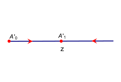
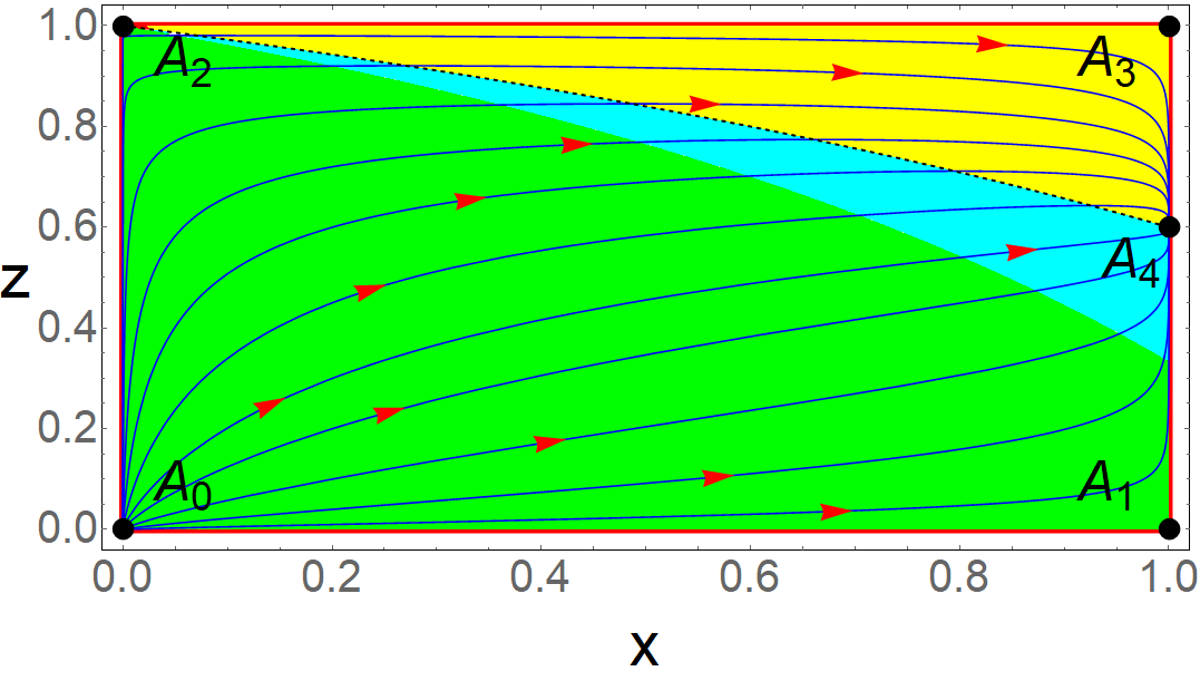
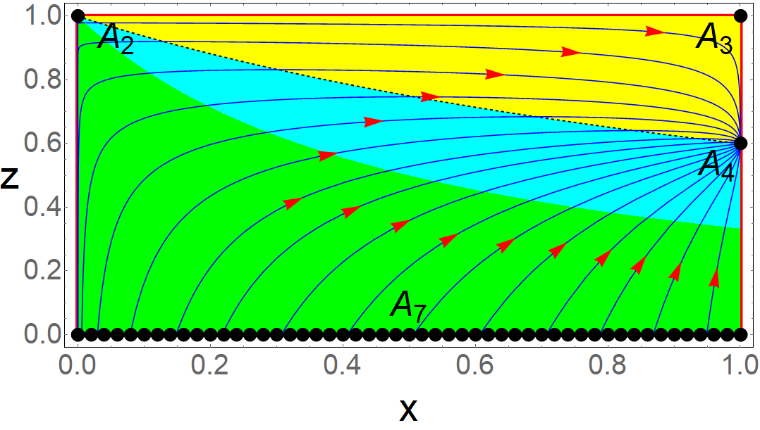
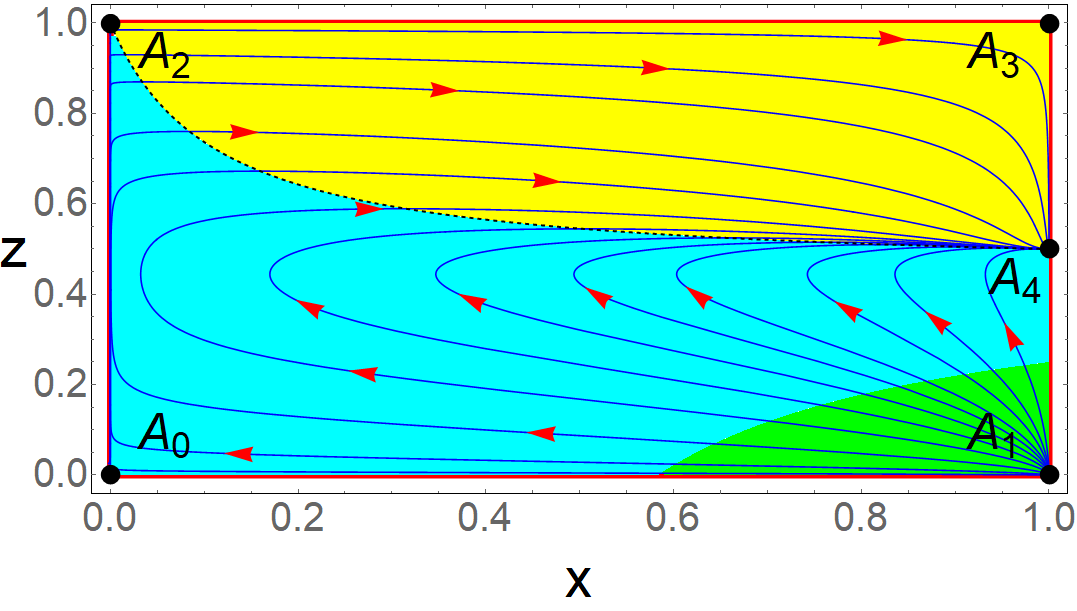
Figure 1: Description of the phase space of the matter creation scenarios (one fluid and two-fluid systems) in which the matter creation rate is constant, i.e. $\Gamma=\Gamma_{0}$. Upper Left Plot: This is the vector plot of the one dimensional system (27). Here, we adopt $\alpha=3$ but for other values of $\alpha>0$ similar type of plot can be found . Upper Right Plot: The phase plot of the system (29) when we have assumed $w=1.5$ and $\alpha=2$. For other values of $w>0$ and $\alpha>0$, we can also obtain similar phase space structure. Lower Left Plot: The phase space of the system (29) when the equation of state $w$ takes the value $0$. Here we use $\alpha=2$ but any positive value of $\alpha$ gives same type of phase portrait. Lower Right Plot: The phase plot of the system (29) considering $w=-0.8$ and $\alpha=3$. Also, we can get similar type of graphics for any positive value of $\alpha$ and negative value of $w$ in the interval $(-1,0)$. In all three two-dimensional plots, green region corresponds to the decelerating phase ($q>0$), cyan region represents the accelerating phase with $-1<q<0$ and the yellow region corresponds to the super accelerating phase (i.e. $q<-1$). The black dotted curve separating the cyan and yellow regions corresponds to $q=-1$.

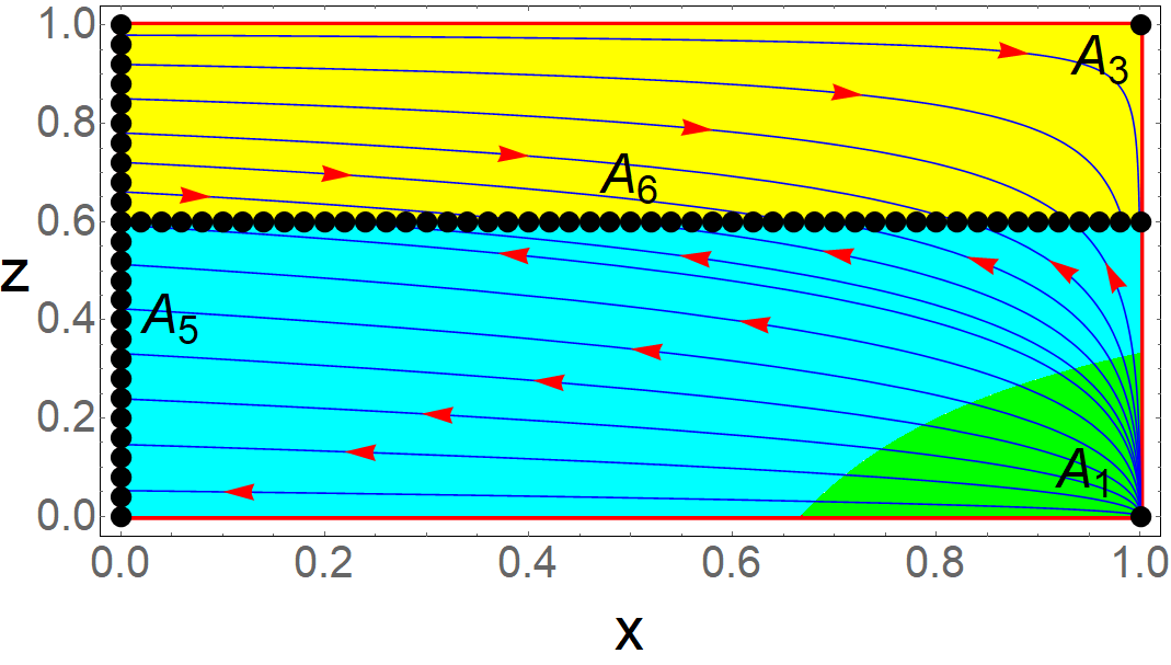
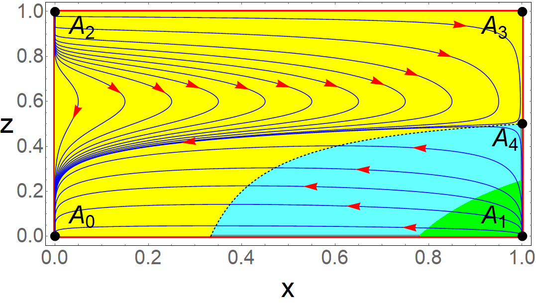
Figure 2: This figure depicts the phase space of the two-fluid system for the constant matter creation rate $\Gamma=\Gamma_{0}$ but here we consider the case with $w\leq-1$. Left Plot: The phase space of the system (29) when the equation of state $w$ takes the value $-1$. Here we use $\alpha=3$ but any positive value of $\alpha$ gives similar type of phase portrait. Right Plot: The phase plot of the system (29) when we assume $w=-1.5$ and $\alpha=3$. For other values of $w<-1$ and $\alpha>0$, we can also obtain similar graphics. In both the plots, green region corresponds to the decelerating phase ($q>0$), cyan region represents the accelerating phase with $-1<q<0$ and the yellow region corresponds to the super accelerating phase (i.e. $q<-1$). The black dotted curve separating the cyan and yellow regions (in the left plot, this separating curve is not visible because of the line of critical points) corresponds to $q=-1$.

1. When $w>0$: In this case, we obtain five critical points, namely, $A_{0}$, $A_{1}$, $A_{2}$, $A_{3}$ and $A_{4}$ which always exist in our region $R_{1}$. Eigenvalues evaluated at $A_{0}$ are $3w$, $\frac{3}{2}(1+w)$ which are positive, hence, this indicates that $A_{0}$ is an unstable critical point dominated by the normal fluid and it represents a decelerating phase of the universe. At $A_{1}$, the eigenvalues are $-3w$, $\frac{3}{2}$, that means one eigenvalue is positive while the other is negative (since $w>0$). So, the critical point $A_{1}$ is saddle in nature which corresponds to the DM dominated decelerating phase. The critical point $A_{2}$ has one eigenvalue $0$. So, we cannot say about stability by applying the linear stability theory and that is why we have applied the center manifold theory. The center manifold is $x=0$ which coincides with the eigenvector ($z$ axis) corresponding to a zero eigenvalue. Clearly, $z^{\prime}$ is positive along $z$ axis which gives $A_{2}$ another saddle point. As the decelerating parameter is undefined at $A_{2}$, hence, we are unable to predict whether this represents an accelerating phase or the reverse. Since, $A_{3}$ has two eigenvalues $-\alpha$, $\frac{\alpha}{2}$ and they are of opposite signs, we can conclude that it is a saddle point. This critical point is a DM dominated accelerated solution. The most interesting critical point is $A_{4}$ which has $\Omega_{dm}=1$ and $q=-1$, i.e. DM dominated accelerating solution. As both the eigenvalues are negative, the critical point $A_{4}$ is the only globally stable point in our domain which is shown in the upper right plot of Fig. 1 where all orbits leave the decelerating phase, then enter into an accelerating phase and finally end in a DM dominated accelerating phase $(q=-1)$. Besides these features we observe that a set of orbits crosses the $q=-1$ curve, enter into a super accelerating phase $(q<-1)$ and finally finish with $q=-1$ phase, which indicates the slowing down of the cosmic acceleration.

2. When $w=0$: In this scenario besides the three isolated critical points $A_{2},~A_{3}$ and $A_{4}$ given in Table 1, we find one critical line $A_{7}(x_{c},0)$ for which the critical points $A_{0}$, $A_{1}$ lie in this critical line. In the phase space $R_{1}$, one can obtain $z^{\prime}>0$ and $z^{\prime}<0$ for $z<\frac{3}{3+\alpha x}$ and for $z>\frac{3}{3+\alpha x}$ respectively, and $x^{\prime}$ takes always positive value (since $\alpha>0$). By the above argument, one can conclude that the critical line $A_{7}$ shows unstable nature, $A_{1},~A_{2}$ behave like saddle points and $A_{3}$ is the only globally stable point. Here, $A_{3},~A_{4}$ correspond to accelerating phase and $A_{7}$ gives decelerating phase, while decelerating parameter is undefined at $A_{2}$. The phase space diagram is highlighted in the lower left plot of the Fig. 1 where one can notice that the universe exits from its past decelerating phase and enters into the DM dominated accelerating phase. Along with these results, a set of orbits traverses the decelerating phase $(q>0)$, then enters into an accelerating phase with $-1<q<0$ but successively these orbits enter into a super accelerating phase $(q<-1)$, and finally the acceleration slows down and it continues with $q=-1$.

3. When $-\frac{1}{3}\leq w<0$: In this interval of $w$, the dynamical system (29) gives five critical points, namely, $A_{0},~A_{1},~A_{2},~A_{3}$ and $A_{4}$. Now we can conclude about the stability of the critical points via investigation of the sign of the eigenvalues and the direction of the flow on the boundary of the unit square. It is clear that $A_{0},~A_{2},~A_{3}$ are saddle by behavior and $A_{1}$ is unstable. Here, $A_{4}$ is the only globally stable point in the phase space. The critical points $A_{3},~A_{4}$ correspond to matter dominated accelerating phases, while $A_{1}$ represents the matter dominated decelerating phase. Note that, $A_{0},~A_{2}$ both are second fluid dominated critical points but again $A_{0}$ shows deceleration and we can not say about the acceleration at $A_{2}$. The phase space trajectories are similar to the lower right plot of the Fig. 1. In this case, the universe quits its past DM dominated decelerating phase and closes in accelerating DM dominated phase. Again, some special orbits tracing accelerating phase $(-1<q<0)$ and super accelerating phase $(q<-1)$, finish in the phase where $q=-1$. The slowing down of cosmic acceleration is also realized in this case.

4. When $-1<w<-\frac{1}{3}$: This case is similar to the above case where $w$ lies in the interval $\left[-\frac{1}{3},0\right)$. The only difference with the above case is in the decelerating parameter where in the above case we get $q\geq 0$ at $A_{0}$ but here, $q<0$ at $A_{0}$ which represents acceleration. The lower right plot of Fig. 1 exhibits the qualitative features of the critical points.

5. When $w=-1$: In this case, we have two critical lines $A_{5}(0,z_{c})$ and $A_{6}\left(x_{c},\frac{3}{3+\alpha}\right)$ along with the critical points $A_{0},~A_{1},~A_{2},~A_{3},~A_{4}$ depicted in the Table 1. Here, $A_{0},~A_{2}$ belong to the critical line $A_{5}$ and $A_{6}$ contains the point $A_{4}$. In the phase space above the $z=3/(3+\alpha)$ line, $x^{\prime}$, $z^{\prime}$ are positive and negative respectively, and below the line $z=3/(3+\alpha)$, $x$ and $z$ are decreasing and increasing respectively. Again, the separatrix $z=\frac{3}{\alpha}(1-z)\sqrt{1-x}$ connecting the critical points $A_{1}$ and $\left(0,3/(3+\alpha)\right)$ divide the phase space below the line $z=3/(3+\alpha)$ into two regions: the orbits below the separatrix converge to the part of the critical line $A_{5}$ where $z<\frac{3}{3+\alpha}$ and the orbits above the separatrix approach the critical line $A_{6}$. As a result, $A_{6}$ behaves like an accelerating late-time attractor where DM and DE both may co-exist. So, the critical point $A_{6}$ has the potentiality to alleviate the coincidence problem. Again, the critical line $A_{5}$ where $z>\frac{3}{3+\alpha}$ are unstable in nature but the part of the critical line $A_{5}$ with $z<\frac{3}{3+\alpha}$ represent late time accelerating attractor dominated by the DE only. The point $A_{3}$ is saddle which shows matter dominated accelerated phase, while $A_{1}$ corresponds to matter dominated decelerating unstable point. The qualitative behavior are highlighted in the left plot of Fig. 2. Here, we have two possibilities: one is, above the separatrix, our universe shows the transition from its past DM dominated decelerating phase to the accelerating scaling solutions and on the other hand, below the separatrix, the universe follows DM dominated decelerating phase to completely DE dominated accelerating phase.

6. When $w<-1$: If the equation of state $w$ of the second fluid lies in the phantom region, we again obtain five critical point which are shown in Table  1, i.e. $A_{0},~A_{1},~A_{2},~A_{3}$ and $A_{4}$. Since the eigenvalues are both negative at $A_{0}$, this is a stable point that exhibits dark-energy dominated accelerated universe. Being two eigenvalues, positive at $A_{1}$, this point is unstable which leads to the matter dominated decelerating phase of the universe. Clearly, the points $A_{0},~A_{2}$ properly describe the phase of the universe. Again, as eigenvalues are opposite in sign evaluated at $A_{3},~A_{4}$, these two critical points are saddle by nature representing acceleration with completely matter domination. Clearly, $A_{2}$, dark-energy dominated point is unstable because one can easily check that $x^{\prime}$, $z^{\prime}$ are both positive on $z=1$ and $x=0$, respectively. The right plot of Fig. 2 exhibits the phase space behavior where a class of orbits leave the decelerating phase and end in the super accelerating phase which is expected in the phantom cosmology.

III.2 Model: $\Gamma=\Gamma_{0}H$

Here, we consider the particle creation rate, $\Gamma=\Gamma_{0}H$ where $\Gamma_{0}$ is a positive constant. In the following we analyze its effects on the universe evolution for both the systems, i.e. one fluid system and two-fluid system.

III.2.1 One fluid system

This is a special matter creation rate in which the decelerating parameter, $q=\frac{1}{2}(1-\Gamma_{0})$ depends only on the free parameter $\Gamma_{0}$, and hence, one can see that universe experiences an accelerating phase for $\Gamma_{0}>1$ or a decelerating phase for $\Gamma_{0}<1$. Note that for any other matter creation model, $q$ will depend on the $z$ variable. Now, here only $z$ variable given in (24) leads to the one dimensional autonomous dynamical system in the form:

$$z^{\prime}=\frac{3}{2}z(1-z)\left(1-\frac{\Gamma_{0}}{3}\right).$$ (30)

Clearly we have two critical points, namely, $B^{\prime}_{0}(1,0)$ and $B^{\prime}_{1}(1,1)$, where first and second components of each critical point are related to DM density parameter and values of $z$ variable, respectively. It is obvious from the above dynamical system that $z$ is increasing and decreasing depending on the parameter $\Gamma_{0}<3$ and $\Gamma_{0}>3$, respectively. So, $B^{\prime}_{0}$ shows unstable nature if $\Gamma_{0}<3$ and stable nature if $\Gamma_{0}>3$, while $B^{\prime}_{1}$ gives stable character if $\Gamma_{0}<3$ and unstable character if $\Gamma_{0}>3$. Again, when $\Gamma_{0}=3$, all points in the phase space (i.e. closed interval $[0,1]$) are critical points showing acceleration. All the information about this model are depicted in Table 2 and the vector plots of the system (30) are exhibited in the Fig. 3. Here, both the critical points simultaneously lie either in the accelerating phase (for $\Gamma_{0}>1$) or decelerating phase $(0<\Gamma_{0}<1)$. For $\Gamma_{0}>3$ we also have physical solutions because $q$ is less than $-1$, and $B^{\prime}_{0}(H\longrightarrow+\infty)$ is stable and $B^{\prime}_{1}(H\longrightarrow 0)$ is unstable. Here we can only conclude that our universe ends in an accelerating phase or a decelerating phase for ($1<\Gamma_{0}$, $\Gamma_{0}\neq 3$) or $(0<\Gamma_{0}<1)$, respectively.

III.2.2 Two fluid system

For this model, using the cosmological equations and the dimensionless variables $x$, $z$ which are mentioned in (24), we obtain the autonomous dynamical system in terms of the dimensionless variables as

$$x^{\prime}= \left(3w+\Gamma_{0}\right)x(1-x),$$ (31a)

$$z^{\prime}= \frac{3}{2}z(1-z)\bigg{[}1+w(1-x)-\frac{\Gamma_{0}}{3}x\bigg{]},$$ (31b)

where $\Gamma_{0}$ is a positive constant. The dynamical system is free from singularity. One can clearly see that the above system has four invariant manifolds $x=0,~x=1,~z=0$ and $z=1$ which make the phase space domain, namely, $R_{2}=[0,1]^{2}$ positively invariant set. In this model the decelerating parameter takes the form $q=\frac{1}{2}\left[1+3w(1-x)-\Gamma_{0}x\right]$ which does not contain the $z$ variable, and for $\left(1-\Gamma_{0}\right)x+(1+3w)(1-x)<0$, the accelerating expansion of the universe is realized. In the Table 2, we properly present the inherent property of the dynamical system (31) (i.e. critical points and different values of the cosmological parameters at these critical points). Since the evolution of $x$ variable significantly depends on the factor $\left(3w+\Gamma_{0}\right)$ for which we carry out the phase space analysis in three possible ways, such as

1. When $3w+\Gamma_{0}<0$: In this case, one can notice from Table 2 that there are four isolated critical points $B_{0},~B_{1},~B_{2},~B_{3}$ and two critical lines $B_{4}$(if $w=-1$), $B_{5}$  (if $\Gamma_{0}=3$). Here, at late times, $x$ goes to zero, and then, at late times, we will have $z^{\prime}=\frac{3}{2}z(1-z)(1+w)$. Thus, the following sub-cases will appear:

   1. $w<-1:$

      1. $\Gamma_{0}\neq 3:$ In this situation, the system has only four isolated critical points, namely, $B_{0},~B_{1},~B_{2},~B_{3}$. At late times, $z$ goes to zero, concluding that $B_{0}$ is a global attractor. Again, examining the eigenvalues, one can conclude that $B_{1}$ is saddle for $\Gamma_{0}>3$ and unstable for $\Gamma_{0}<3$, $B_{2}$ is always saddle in nature, $B_{3}$ is unstable if $\Gamma_{0}>3$ and saddle by behavior if $\Gamma_{0}<3$. Here, $B_{0},~B_{2}$ always lie in the accelerated region while $B_{1},~B_{3}$ remain in the accelerated phase if $\Gamma_{0}>1$. So we can conclude that $B_{0}$ is the late time DE dominated accelerating global attractor and universe undergoes from decelerating to accelerating phase if we choose the model parameter $\Gamma_{0}<1$. This scenario is depicted in the lower right plot of the Fig. 4.

      2. $\Gamma_{0}=3:$ Along with two isolated critical points $B_{0},~B_{2}$, we have one critical line $B_{5}$, containing the critical points $B_{1},~B_{3}$. As one eigenvalue is positive and other is zero, $B_{5}$ behaves like unstable point. All the critical points and line are representing accelerating solutions. Once again, $B_{0}$ is the only late time DE dominated global attractor which we have seen in the previous paragraph.

   2. $w=-1:$ When the equation of state of the second fluid coincides with cosmological constant $(w=-1)$, one can get two critical points and one critical line, namely, $B_{1},~B_{3}$ and $B_{4}$. Now, we have $z^{\prime}=\frac{3}{2}z(1-z)x\left(1-\frac{\Gamma_{0}}{3}\right)$. Taking into account that $1-\frac{\Gamma_{0}}{3}>0$, we deduce that $z$ is an increasing function, concluding that $B_{4}$ behaves like stable in nature. The line $B_{4}$ is always accelerated while $B_{1},~B_{3}$ are accelerated for $\Gamma_{0}>1$ otherwise decelerated. Thus, one may conclude that the universe leaves early time matter dominated decelerated phase for $\Gamma_{0}<1$ and ends with completely DE dominated accelerated phase (see lower left plot of Fig. 4).

   3. $-1<w<0:$ In this interval of $w$, the system (31) provides four isolated critical points $B_{0},~B_{1},~B_{2}$ and $B_{3}$. In this situation, at late times, $z$ goes to $1$. Thus, $B_{2}$ is a global attractor. Here, one can deduce that $\Gamma_{0}<3$ for which, the nature of eigenvalues indicate that $B_{0}$ is saddle point, $B_{1}$ is unstable in $\Gamma_{0}<3$, and $B_{3}$ is saddle in $\Gamma_{0}<3$. The point $B_{0},~B_{2}$ correspond to accelerating epoch for $w<-1/3$ and $B_{1},~B_{3}$ represents accelerating epoch in $\Gamma_{0}>1$. If $w$ mimics the quintessential DE equation of state (i.e. $-1<w<-1/3$) with $\Gamma_{0}<1$, we obtain the proper evolution of the universe.

2. When $3w+\Gamma_{0}=0$: Now $x^{\prime}=0$, meaning that the trajectories are the straight lines $x=$ constant. The equation for $z$ becomes $z^{\prime}=\frac{3}{2}z(1-z)(1+w)$ and the decelerating parameter takes the form $q=(1+3w)/2$ which implies that all points in the phase space are accelerated for $w<-1/3$ and decelerated for $-1/3<w<0$.

   1. $w<-1:$ In this phantom region of $w$, we have extracted two critical lines, namely, $B_{6}$, $B_{7}$, where DE and DM coexist. Here, $z$ is decreasing, deducing that for $w<-1$, $z$ goes to $0$. Thus $B_{6}$ gives stable character and $B_{7}$ shows unstable qualitative behavior, which are verified using the eigenvalues (see Table 2).

   2. $w=-1:$ When $w=-1$ i.e. $\Gamma_{0}=3$, we we have $z^{\prime}=0$, that is, all the points of the phase space are critical points and they are accelerated.

   3. $-1<w<0:$ Finally when $w>-1$, once again we have found two critical lines $\left(B_{6},B_{7}\right)$, having both DE and DM. From the evolution of $z$, one can conclude, $z$ is increasing i.e. $z$ goes to $1$. Therefore, $B_{7},~B_{6}$ behave like an attractor and a repeller respectively. These are also checked by eigenvalues (see Table 2). The phase plot is shown in the upper right plot of the Fig. 4.

3. When $3w+\Gamma_{0}>0$: In that case, at late times, $x$ goes to $1$, and, at late times, the equation for $z$ will become: $z^{\prime}=\frac{3}{2}z(1-z)\left(1-\frac{\Gamma_{0}}{3}\right)$. Here, it will appear the following situations:

   1. $0<\Gamma_{0}<3:$ Here, one can verify that $w>-1$. In that case, the dynamical system (31) produces four critical points $B_{0},~B_{1},~B_{2},~B_{3}$. As $z^{\prime}>0$, $z$ goes to $1$, and thus, $B_{3}$ is a global attractor. Again, $B_{0}$ is unstable and $B_{1},~B_{2}$ are saddle by behavior. If $-1/3<w$ and $\Gamma_{0}>1$, the evolution scenario is at early phase, orbits leaves from second fluid dominated decelerating phase and ends in DM dominated accelerating phase (see upper left plot of Fig. 4).

   2. $\Gamma_{0}=3:$ Here, one can easily find two isolated critical points $B_{0},~B_{2}$ and one critical line $B_{5}$. Now, we will have $z^{\prime}=\frac{3}{2}z(1-z)(1+w)(1-x)$. Taking into account that, $w>-1$, we conclude that $B_{5}$ behaves like a global attractor. From the sign of eigenvalues, we can determine the stability of $B_{0},~B_{2}$ ($B_{0}$ is unstable and $B_{2}$ is saddle). Therefore, the final state of the universe is DM dominated accelerating phase.

   3. $\Gamma_{0}>3:$ In that case, once again, there are four critical points $B_{0},~B_{1},~B_{2},~B_{3}$ in the phase space. Since, $z$ goes to $0$, and thus, $B_{1}$ is a global attractor. From the point of view of the nature of eigenvalues, $B_{3}$ is always saddle, $B_{0}$ is unstable where $B_{2}$ is saddle, and $B_{2}$ is unstable where $B_{0}$ is saddle. Here, we can observe that $B_{0},~B_{2}$ for $w<-1/3$ and $B_{1},~B_{3}$ always, lie in the accelerating phase.

		One fluid system
Critical point		Existence	Stability		$\Omega_{\rm dm}$	$q$	Acceleration
$B^{\prime}_{0}(1,0)$		Always	Stable if $\Gamma_{0}>3$ and		1	$\frac{1}{2}(1-\Gamma_{0})$	$\Gamma_{0}>1$
			Unstable if $\Gamma_{0}<3$
$B^{\prime}_{1}\left(1,1\right)$		Always	Stable if $\Gamma_{0}<3$ and		1	$\frac{1}{2}(1-\Gamma_{0})$	$\Gamma_{0}>1$
			Unstable if $\Gamma_{0}>3$
$B^{\prime}_{2}\left(1,z_{c}\right)$		$\Gamma_{0}=3$	All are critical points		$1$	$-1$	Yes
		Two fluid system
Critical point	Existence	Eigenvalue	Stability	$\Omega_{f}$	$\Omega_{\rm dm}$	$q$	Acceleration
$B_{0}(0,0)$	Always	$\left(3w+\Gamma_{0},\frac{3}{2}(1+w)\right)$	Stable if $3w+\Gamma_{0}<0,~w\leq-1$	$1$	$0$	$\frac{1}{2}(1+3w)$	$w<-\frac{1}{3}$
			and if $3w+\Gamma_{0}=0,~w<-1$;
			Otherwise Unstable or Saddle
$B_{1}(1,0)$	Always	$\left(-(3w+\Gamma_{0}),\frac{3-\Gamma_{0}}{2}\right)$	Stable if $3w+\Gamma_{0}>0,~\Gamma_{0}\geq 3$	$0$	$1$	$\frac{1}{2}(1-\Gamma_{0})$	$\Gamma_{0}>1$
			and if $3w+\Gamma_{0}=0,~\Gamma_{0}>3$;
			Otherwise Unstable or Saddle
$B_{2}(0,1)$	Always	$\left(3w+\Gamma_{0},-\frac{3}{2}(1+w)\right)$	Stable if $3w+\Gamma_{0}<0,~w\geq-1$	$1$	$0$	$\frac{1}{2}(1+3w)$	$w<-\frac{1}{3}$
			and if $3w+\Gamma_{0}=0,~w>-1$;
			Otherwise Unstable or Saddle
$B_{3}(1,1)$	Always	$\left(-(3w+\Gamma_{0}),\frac{\Gamma_{0}-3}{2}\right)$	Stable if $3w+\Gamma_{0}>0,~\Gamma_{0}\leq 3$	$0$	$1$	$\frac{1}{2}(1-\Gamma_{0})$	$\Gamma_{0}>1$
			and if $3w+\Gamma_{0}=0,~\Gamma_{0}<3$;
			Otherwise Unstable or Saddle
$B_{4}\left(0,z_{c}\right)$	$w=-1$	$\left(\Gamma_{0}-3,0\right)$	Stable if $\Gamma_{0}<3$ and	$1$	$0$	$-1$	Yes
			Unstable if $\Gamma_{0}>3$
$B_{5}\left(1,z_{c}\right)$	$\Gamma_{0}=3$	$\left(-3(1+w),0\right)$	Stable if $w>-1$ and	$0$	$1$	$-1$	Yes
			Unstable if $w<-1$
$B_{6}\left(x_{c},0\right)$	$3w+\Gamma_{0}=0$	$\left(0,\frac{3-\Gamma_{0}}{2}\right)$	Stable if $\Gamma_{0}>3$ and	$1-x_{c}$	$x_{c}$	$\frac{1}{2}(1+3w)$	$w<-\frac{1}{3}$
			Unstable if $\Gamma_{0}<3$
$B_{7}\left(x_{c},1\right)$	$3w+\Gamma_{0}=0$	$\left(0,\frac{\Gamma_{0}-3}{2}\right)$	Stable if $\Gamma_{0}<3$ and	$1-x_{c}$	$x_{c}$	$\frac{1}{2}(1+3w)$	$w<-\frac{1}{3}$
			Unstable if $\Gamma_{0}>3$
$B_{8}\left(x_{c},z_{c}\right)$	$w=-1,~\Gamma_{0}=3$	$(0,0)$	All points in the phase	$1-x_{c}$	$x_{c}$	$-1$	Yes
			space are critical points

Table 2: Summary of the critical points, their existence, stability and the values of the cosmological parameters at those points for the dynamical system (30) and (31) with the matter creation rate $\Gamma=\Gamma_{0}H$.

Figure 3: Left Plot: This is the vector plot of the one dimensional system (30), i.e. for the model $\Gamma=\Gamma_{0}H$, considering positive $\Gamma_{0}$ with $\Gamma_{0}<3$. Right Plot: This is the vector plot of the one dimensional system (30) considering positive $\Gamma_{0}$ with $\Gamma_{0}>3$.

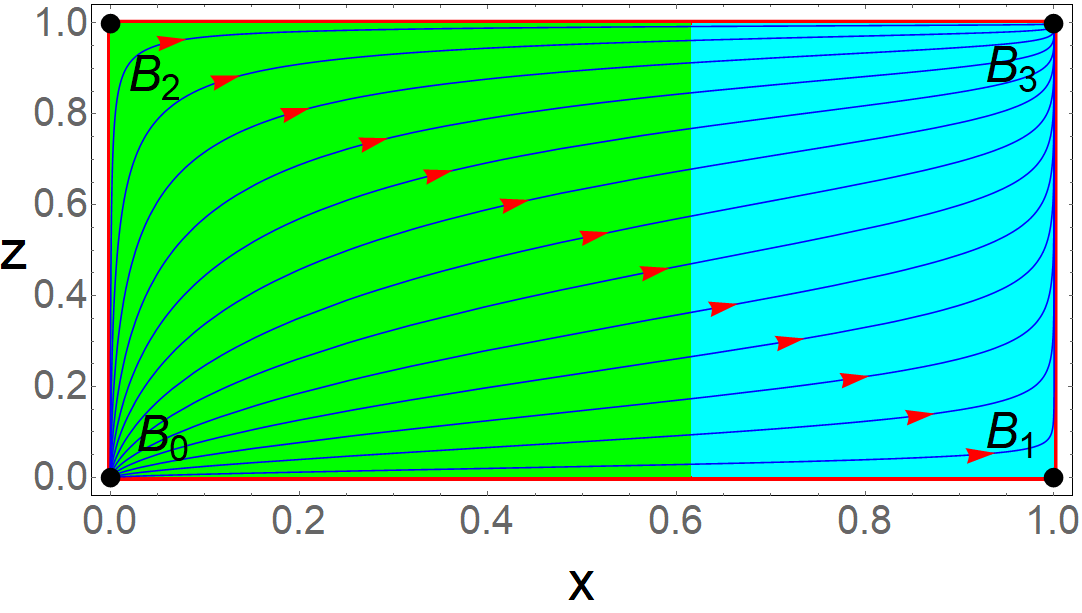
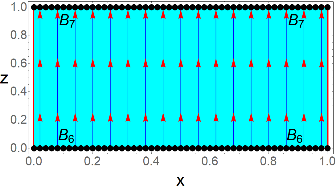
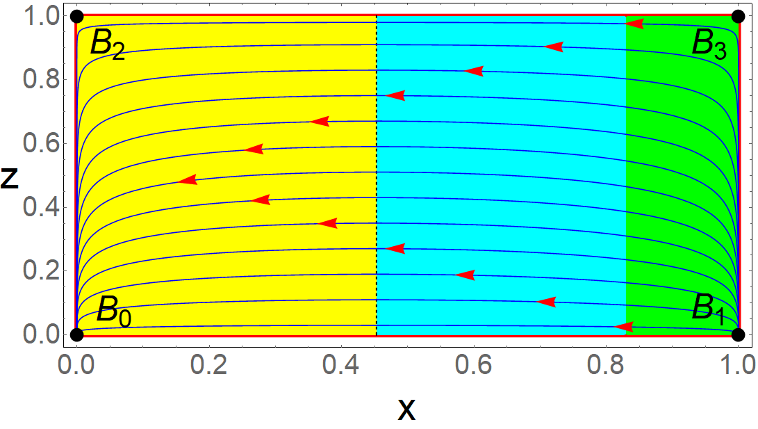
Figure 4: Description of the phase space of the two-fluid system for the matter creation rate $\Gamma=\Gamma_{0}H$. Upper Left Plot: The phase plot of the system (31) assuming $w=0.2$ and $\Gamma_{0}=2$. If we take any value of $w$ from $w>-1$ and $\Gamma_{0}$ in the region $0<\Gamma_{0}<3$, satisfying $3w+\Gamma_{0}>0$, we can get similar plot. Upper Right Plot: The phase plot of the system (31) for $-1<w<0$ satisfying $3w+\Gamma_{0}=0$. Here when we have assumed $w=-0.8$ and $\Gamma_{0}=2.4$, however, any value of $w$ lying in $(-1,0)$ and any positive value of $\Gamma_{0}$ satisfying the above condition will give similar plot. Lower Left Plot: The phase plot of the system (31) when the equation of state of the second fluid $w$ adopts the value $w=-1$. In this context, we choose $\Gamma_{0}=0.2$ but any positive value of $\Gamma_{0}$ satisfying $3w+\Gamma_{0}<0$ produces similar type of phase space diagram. Lower Right Plot: This is the phase plot of the system (31) for $w<-1$ satisfying $3w+\Gamma_{0}<0$. Here we use $w=-1.8$ and $\Gamma_{0}=0.1$ for drawing the graphics, however, any typical value of $w<-1$ and any positive value of $\Gamma_{0}$ $(\Gamma_{0}\neq 3)$ will give similar plot. Here the green region corresponds to the decelerating phase ($q>0$), cyan region represents the accelerating phase with $-1<q<0$ and the yellow region corresponds to the super accelerating phase ($q<-1$). In the lower right graph, the vertical black dotted line corresponds to $q=-1$.

III.3 Model: $\Gamma=\Gamma_{0}H^{2}$

In this case, we have constructed the model considering the particle creation rate $\Gamma=\Gamma_{0}H^{2}$ where $\Gamma_{0}$ is a constant having dimension of the inverse of the Hubble rate. We shall also discuss how $\Gamma$ influences the universe’s evolution for both the fluids.

III.3.1 One fluid system

Following the similar arguments as in the earlier cases with one-fluid system, for this model, the one dimensional autonomous system can be reads as:

$$z^{\prime}=\frac{3}{2}(1-z)\left(z-\frac{\beta(1-z)}{3}\right),$$ (32)

where $\beta=\Gamma_{0}H_{0}$ is the dimensionless constant and it takes positive values. If we solve the quadratic equation $z^{\prime}=0$, we get two critical points, namely, $C^{\prime}_{0}(1,1)$ and $C^{\prime}_{1}\left(1,\frac{\beta}{3+\beta}\right)$, where first and second component of the critical points correspond to dark-matter density parameter and the value of $z$ variable respectively. The point $C^{\prime}_{0}$ is always stable and represents decelerating phase of the universe. Again, $C^{\prime}_{1}$ corresponds to an accelerating phase of the universe whenever $C^{\prime}_{1}$ exists, i.e. $\beta>0$, and this point is always unstable. The directions of the vector field defined in (32) are given in the upper left plot of the Fig. 5. In this case $q=\frac{1}{2}\left(1-\frac{\beta(1-z)}{z}\right)$. Then, the critical point $C^{\prime}_{1}$ corresponds to $q=-1$ that is, a de Sitter solution. At the present time, which corresponds to $z=1/2$, we have $q=\frac{1}{2}(1-\beta)$. Then, to have an acceleration at the present time we need $\beta>1$. On the other hand, for $\beta<3$ we have $\frac{\beta}{\beta+3}<\frac{1}{2}$. Thus, in this situation, the universe passes from an accelerating phase to a decelerating one at the late time. On the contrary, when $\beta>3$, we have $\frac{\beta}{\beta+3}>\frac{1}{2}$, and thus, the universe is always accelerating. Note that when $\beta=3$, the critical point coincides with $1/2$, this means at the present time the universe is in a de Sitter phase. In fact, when $1<\beta<3$, because in this case the universe starts in a de Sitter phase and at the present time it accelerates (finally, at late times it decelerates) always in a non-phantom phase. On the contrary, for $\beta>3$ the universe is always in a phantom phase. This one-fluid system can predict a transition of our universe from the present (or past) accelerating era to future decelerating era.

III.3.2 Two fluid system

In this case, the autonomous system takes the form

$$x^{\prime}= x(1-x)\left(3w+\frac{\beta(1-z)}{z}\right),$$ (33a)

$$z^{\prime}= \frac{3}{2}z(1-z)\left[1+w(1-x)-\frac{\beta x(1-z)}{3z}\right],$$ (33b)

where $\beta=\Gamma_{0}H_{0}$ is a dimensionless and positive constant. The above system has singularity at $z=0$. We multiply to the right hand sides of (33) by $z$ to make the system regularised. After doing this, the regularized system becomes,

$$x^{\prime}= x(1-x)\left(3wz+\beta(1-z)\right),$$ (34a)

$$z^{\prime}= \frac{3}{2}z(1-z)\left[\left(1+w(1-x)\right)z-\frac{\beta x(1-z)}{3}\right].$$ (34b)

From eqn. (24), it is clear that our physical domain is $R_{3}=[0,1]^{2}$ and the dynamical system (34) gives $x=0,~x=1,~z=0,~z=1$ as the invariant manifolds which lead the domain $R_{3}$ to being a positively invariant set. Being $q=\frac{1}{2}\left[1+3w(1-x)-\frac{\beta x(1-z)}{z}\right]$ in this case, the requirement for realizing an accelerating phase at the present moment (i.e. $z=1/2$), the physical trajectories should satisfy the relation $(1-\beta)x+(1+3w)(1-x)<0$. In the following we describe the qualitative features of the above dynamical system for different values of $w$.

		One fluid system
Critical point		Existence	Stability		$\Omega_{\rm dm}$	$q$	Acceleration
$C^{\prime}_{0}(1,1)$		Always	Always Stable		1	$\frac{1}{2}$	No
$C^{\prime}_{1}\left(1,\frac{\beta}{3+\beta}\right)$		$\beta>0$	Always Unstable		1	$-1$	Yes
		Two fluid system
Critical point	Existence	Eigenvalue	Stability	$\Omega_{f}$	$\Omega_{\rm dm}$	$q$	Acceleration
$C_{0}(0,0)$	Always	$(\beta,0)$	Unstable if $w>-1$;	1	0	Undefined	Undetermined
			Non-hyperbolic Saddle if $w<-1$
$C_{1}(1,0)$	Always	$\left(-\beta,-\frac{\beta}{2}\right)$	Stable	0	1	$-\infty$	Yes
$C_{2}(0,1)$	Always	$\left(3w,-\frac{3}{2}(1+w)\right)$	Stable if $-1<w<0$;	1	0	$\frac{1}{2}(1+3w)$	$w<-\frac{1}{3}$
			Saddle if $w<-1$ and if $w>0$
$C_{3}(1,1)$	Always	$\left(-3w,-\frac{3}{2}\right)$	Stable if $w>0$;	0	1	$\frac{1}{2}$	No
			Saddle if $w<0$
$C_{4}\left(1,\frac{\beta}{\beta+3}\right)$	$\beta>0$	$\left(-\frac{3\beta(1+w)}{3+\beta},\frac{3\beta}{2(3+\beta)}\right)$	Saddle if $w>-1$	0	1	$-1$	Yes
			Unstable if $w<-1$
$C_{5}\left(0,z_{c}\right)$	$w=-1$	$\left(\beta-(\beta+3)z_{c},0\right)$	Stable if $z_{c}>\frac{\beta}{\beta+3}$	$1$	$0$	$-1$	Yes
			Unstable if $z_{c}<\frac{\beta}{\beta+3}$
$C_{6}\left(x_{c},\frac{\beta}{\beta+3}\right)$	$w=-1$	$\left(0,\frac{3\beta x_{c}}{2(3+\beta)}\right)$	Unstable	$1-x_{c}$	$x_{c}$	$-1$	Yes
$C_{7}\left(x_{c},1\right)$	$w=0$	$\left(0,-\frac{3}{2}\right)$	Stable	$1-x_{c}$	$x_{c}$	$\frac{1}{2}$	No

Table 3: Summary of the critical points, their existence, stability and the values of the cosmological parameters at those points for the dynamical system (32) and (34) with the matter creation rate $\Gamma=\Gamma_{0}H^{2}$.

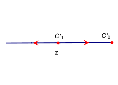
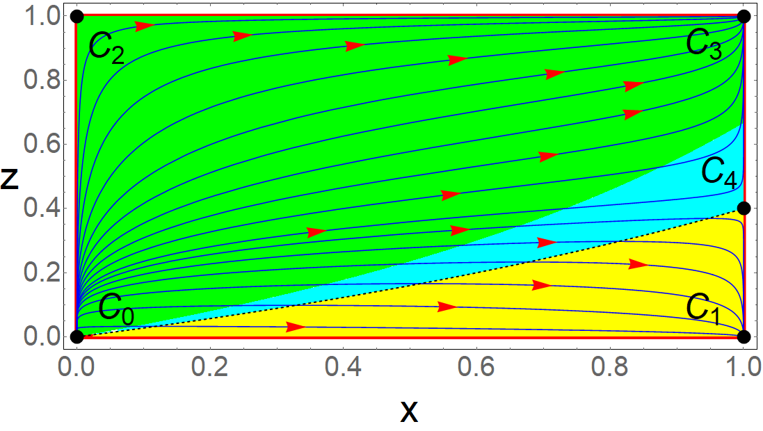
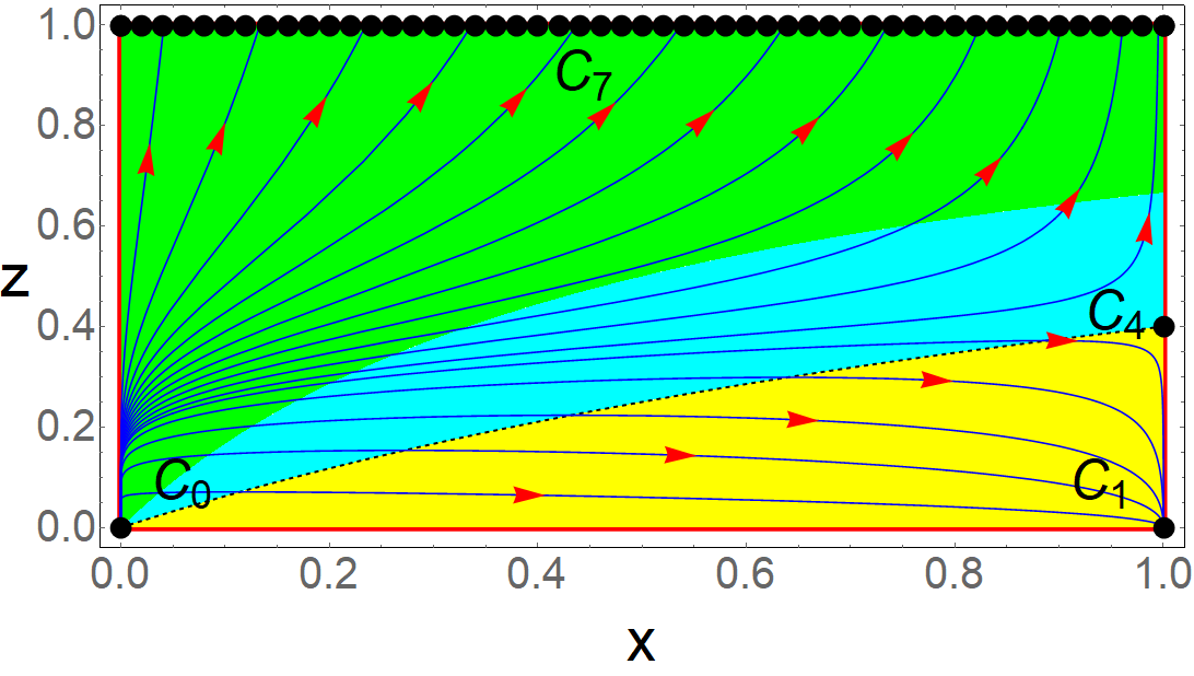
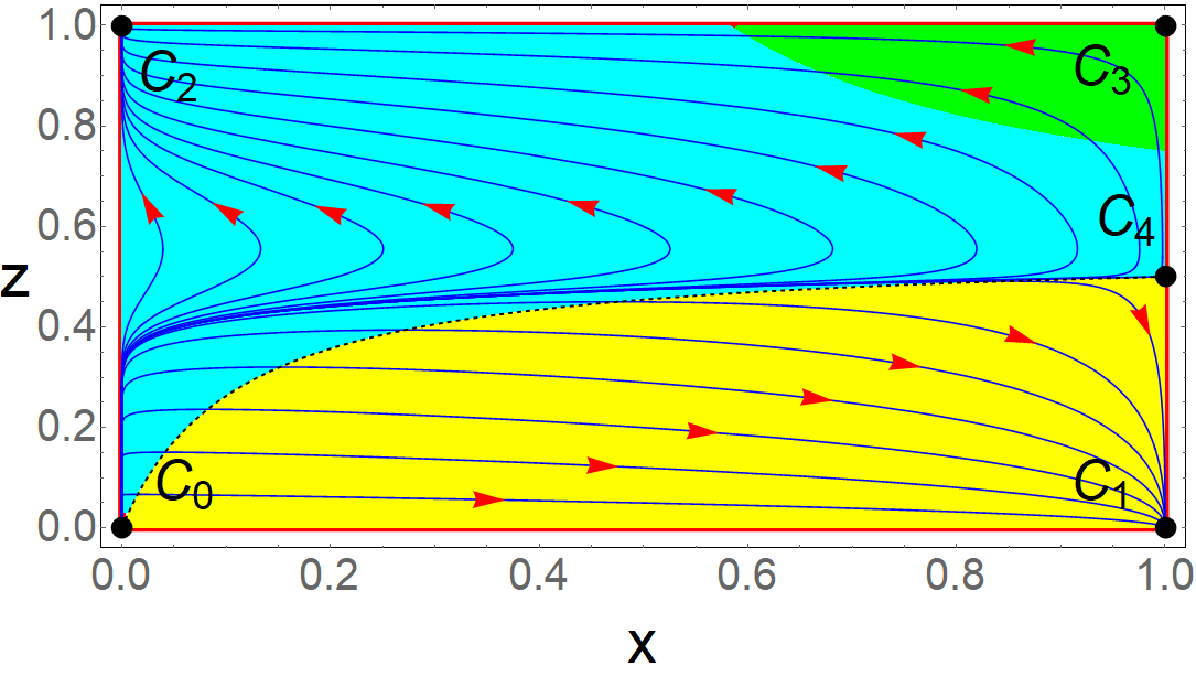
Figure 5: Description of the phase space of the one-fluid and two-fluid systems for the matter creation rate $\Gamma=\Gamma_{0}H^{2}$. Upper Left Plot: This is the vector plot of the one dimensional system (32). Here, we adopt $\beta=3$ but for other values of $\beta>0$ similar type of plot can be found . Upper Right Plot: The phase plot of the system (34) when we have assumed $w=1.5$ and $\beta=2$. For other values of $w>0$ and $\beta>0$, we can also obtain similar phase space structure. Lower Left Plot: The phase space of the system (34) when the equation of state $w$ takes the value $0$. Here we use $\beta=2$ but any positive value of $\beta$ gives same type of phase portrait. Lower Right Plot: The phase plot of the system (34) considering $w=-0.8$ and $\beta=3$. Also, we can get similar type of graphics for any positive value of $\beta$ and negative value of $w$ in the interval $(-1,0)$. Here the green region corresponds to the decelerating phase ($q>0$), cyan region represents the accelerating phase with $-1<q<0$ and the yellow region corresponds to the super accelerating phase (i.e. $q<-1$). In all three two-dimensional graphs, the black dotted curve separating the cyan and yellow regions corresponds to $q=-1$.

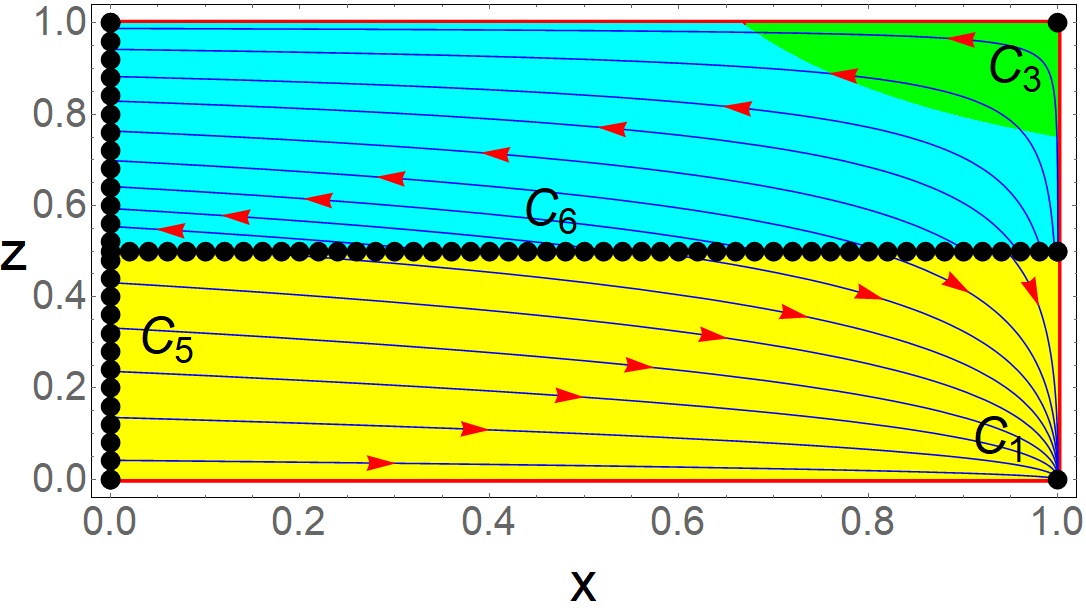
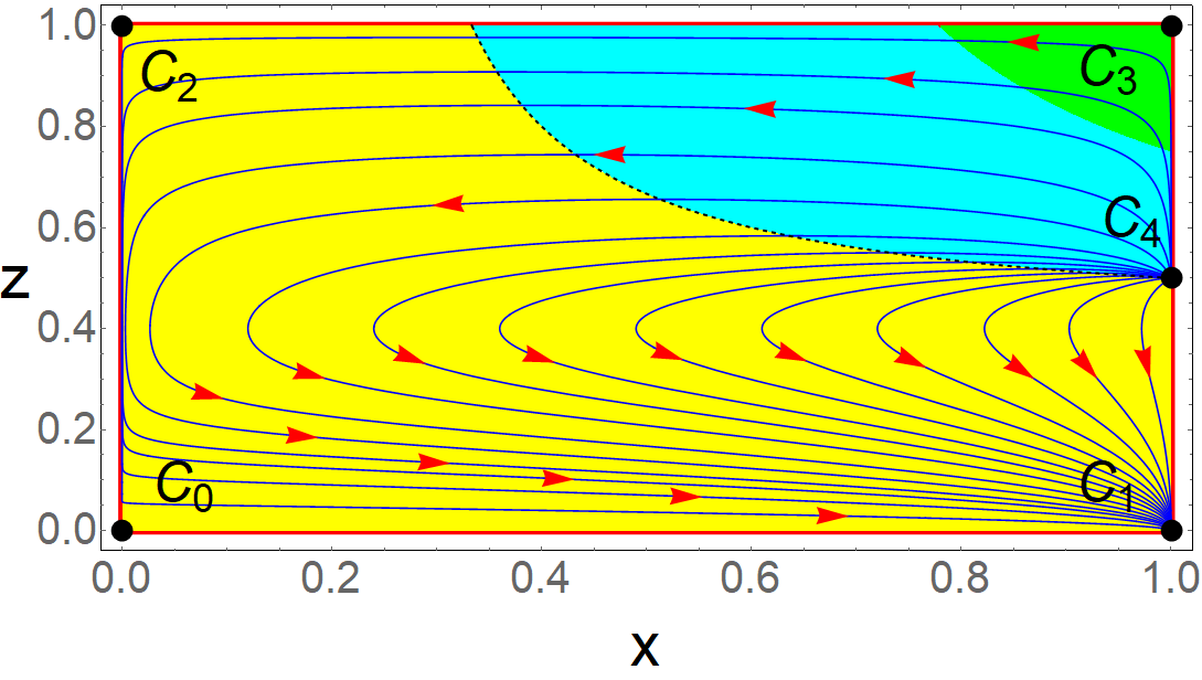
Figure 6: This figure also depicts the phase space of the two-fluid system driven by the matter creation rate $\Gamma=\Gamma_{0}H^{2}$ but here we consider the case when $w\leq-1$. Left Plot: The phase space of the system (34) when the equation of state $w$ takes the value $-1$. Here we use $\beta=3$ but any positive value of $\beta$ gives similar type of phase portrait. Right Plot: The phase plot of the system (34) when we assume $w=-1.5$ and $\beta=3$. For other values of $w<-1$ and $\beta>0$, we can also obtain similar graphics. Here the green region corresponds to the decelerating phase ($q>0$), the cyan region represents the accelerating phase with $-1<q<0$ and the yellow region corresponds to the super accelerating phase (i.e. $q<-1$). The black dotted curve (in the left graph this curve is not visible because of the presence of the critical line) separating the cyan and yellow regions corresponds to $q=-1$.

1. When $w>0$: Considering the equation of state ($w$) of the second fluid as positive, one can get five isolated critical points, namely, $C_{0},~C_{1},~C_{2},~C_{3},~C_{4}$ which are highlighted in the Table 3. Now investigation of eigenvalues assure that $C_{1},~C_{3}$ are stable points and $C_{2},~C_{4}$ are saddle points. Again, eigenvectors corresponding to the eigenvalues $\beta,~0$ at the point $C_{0}$ lie on $x$ and $z$ axis respectively. Since, $x$ is increasing on $z$ axis and $z$ is increasing on $x$ axis, $C_{0}$ behaves like an unstable point. Here, $C_{1},~C_{4}$ belong to the accelerating phase and $C_{2},~C_{3}$ belong to the decelerating phase, while decelerating parameter is undefined at $C_{0}$. Now, the condition to be a viable trajectories are the ones that at $z=1/2$ the deceleration parameter should be negative. This implies $x\left(1-{\beta}\right)+(1+3w)(1-x)<0\Longrightarrow x>\frac{1+3w}{\beta+3w}.$ The upper right plot of the Fig. 5 depicts the complete evolution of the phase space orbits. Here, note that one can trace a set of orbits for which the universe leaves the past decelerating phase, enters in the present (or at finite time) accelerating epoch and ends again in a DM dominated decelerating phase or a DM dominated super accelerating phase.

2. When $w=0$: If we assume the equation of state $w$ is zero, we obtain three isolated critical points $C_{0},~C_{1},~C_{4}$ which are mentioned earlier and one critical line $C_{7}(x_{c},1)$. Again, one can obtain $z^{\prime}>0$, $z^{\prime}<0$ and $x^{\prime}>0$ according to $z>\frac{\beta x}{3+\beta x}$, $z<\frac{\beta x}{3+\beta x}$ and on $z=0$ line, respectively if we choose $\beta$ as positive parameter. Therefore, the above arguments indicate that $C_{7}$ gives stable like nature, $C_{0}$ is unstable, $C_{1}$ is stable and $C_{4}$ is saddle point. Note that $C_{1},~C_{4}$ are accelerated points, but $C_{7}$ represents decelerating phase. The lower left plot of the Fig. 5 highlights the qualitative behavior of this model. It is also noted that the universe leaves its past decelerating phase and then it enters into the current (or at finite time) accelerating phase and finally it again enters into a decelerating phase admitting scaling solutions or a super accelerating phase dominated by DM.

3. When $-\frac{1}{3}\leq w<0$: For these values of $w$, five isolated critical points ($C_{0},~C_{1},~C_{2},~C_{3},~C_{4}$) always belong to our domain $R_{3}$. From the sign of the eigenvalues, one can conclude that $C_{1},~C_{2}$ act like stable points and $C_{3},~C_{4}$ are saddle by nature. As before with similar reason, $C_{0}$ shows unstable character. Depending on the decelerating parameter, $q$, the critical points $C_{1},~C_{4}$ lie in the accelerating phase and $C_{2},~C_{3}$ also lie in the decelerating phase, while we can say nothing about the acceleration of the point $C_{0}$. The phase plot is similar to the lower right plot of the Fig. 5.

   Thus, the final state of the universe is second fluid dominated decelerating phase or DM dominated super accelerating epoch.

4. When $-1<w<-\frac{1}{3}$: The qualitative behavior of the critical points given in the Table 3 are exactly similar to the above scenario where $w$ lies in $-\frac{1}{3}\leq w<0$, which are exhibited in the lower right plot of the Fig. 5. Note that, here the point $C_{2}$ represents acceleration. Here, the fate of the universe is completely DE dominated accelerating epoch or DM dominated super accelerating phase.

5. When $w=-1$: In this case, the dynamical system (33) gives two isolated critical points $C_{1}$, $C_{3}$ which are described in Table 3, and two extra critical lines, namely, $C_{5}(0,z_{c})$ and $C_{6}\left(x_{c},\frac{\beta}{\beta+3}\right)$. There are no restriction on existence of the critical points $C_{1},~C_{3}$ and the critical line $C_{5}$ but the critical line $C_{6}$ belongs to our domain $R_{3}$ only when $\beta$ is taken to be positive. If we look into the evolution of $z$, one can easily find that $z^{\prime}$ is positive and negative when we choose $z>\frac{\beta}{\beta+3}$ and $z<\frac{\beta}{\beta+3}$, respectively. Again, $x$ is increasing below the line $z=\frac{\beta}{\beta+3}$ and it is decreasing above the line $z=\frac{\beta}{\beta+3}$. As a result, $C_{1}$ is stable, $C_{3}$ is always saddle, $C_{6}$ gives unstable behavior, $C_{5}$ is stable for $z_{c}>\frac{\beta}{\beta+3}$ otherwise this line is unstable. Clearly, the critical point $C_{1}$ and the critical line $C_{5},~C_{6}$ lead to the accelerated solution, while $C_{3}$ gives decelerated solution. The phase space structure are clearly visible in the left plot of Fig. 6. Therefore, $C_{5}$ with $z_{c}>\frac{\beta}{\beta+3}$ represents completely DE dominated accelerating solution.

6. When $w<-1$: If we consider the second fluid as dark fluid whose equation of state lie in the phantom region, the critical points for the dynamical system (34) are $C_{0},~C_{1},~C_{2},~C_{3},~C_{4}$ which all are isolated. Inspection of the eigenvalues and the direction of the flow on the $x,~z$ axes, we can easily say that $C_{0},~C_{2},~C_{3}$ are saddle by behavior, $C_{4}$ is unstable and $C_{1}$ is the only globally stable point. Here, $C_{1},~C_{3},~C_{4}$ are matter dominated solutions and $C_{0},~C_{2}$ correspond to completely DE dominated solution. Again, $C_{1},~C_{2},~C_{4}$ are accelerated critical points and $C_{3}$ gives deceleration. The right plot of Fig. 6 shows the correct phase portrait. Although, we assume that the second fluid is phantom-like, however, we do not notice any DE dominated accelerating late time stable point, rather we find DM dominated super accelerating $(q<-1)$ late time stable point.

III.4 Model: $\Gamma=\Gamma_{0}H^{-1}$

In this series of matter creation models, one of the interesting matter creation rate is $\Gamma=\Gamma_{0}H^{-1}$, where $\Gamma_{0}$ is constant having dimension equal to the dimension of the square of the Hubble rate. In the following we describe the influence of this model on both one-fluid and two-fluid systems.

III.4.1 One fluid system

The dynamics of the matter creation model in the one-fluid system is described by the following differential equation

$$z^{\prime}=\frac{3}{2}z\left(1-z-\frac{\gamma z^{2}}{3(1-z)}\right)$$ (35)

where $\gamma=\Gamma_{0}/H_{0}^{2}$ is a positive dimensionless constant and as one can notice the above equation admits one singularity at $z=1$. Therefore, we regularize the above equation and after regularization, it becomes

$$z^{\prime}=\frac{3}{2}z\left((1-z)^{2}-\frac{\gamma z^{2}}{3}\right).$$ (36)

The decelerating parameter $q=\frac{1}{2}\left[1-\frac{\gamma z^{2}}{(1-z)^{2}}\right]$ at present epoch (i.e. $z=1/2)$ takes the form $q=\frac{1-\gamma}{2}$ from which one derives that at present time accelerating expansion of the universe needs $\gamma>1$. We evaluate the critical points of this one dimensional system and in Table 4 we present them along with their qualitative features. Each critical point represents an ordered pair where the first component denotes the DM density parameter and the second component is related to the $z$ variable. The critical point $D^{\prime}_{0}(1,0)$ is always unstable and it represents matter dominated decelerating phase. Again, $D^{\prime}_{1}\left(1,\frac{1}{1+\sqrt{\frac{\gamma}{3}}}\right)$ represents the matter dominated accelerating attractor. The one dimensional vector field involved in the equation (36) is displayed in the upper left plot of Fig. 7. This model gives the transition of our universe from its past $(H\longrightarrow+\infty)$ decelerating phase to the current (or at finite time where $H$ adopts finite value) accelerating phase.

III.4.2 Two fluid system

For this matter creation model, the two dimensional autonomous system becomes

$$x^{\prime}= x(1-x)\left(3w+\frac{\gamma z^{2}}{(1-z)^{2}}\right),$$ (37a)

$$z^{\prime}= \frac{3}{2}z(1-z)\left[1+w(1-x)-\frac{\gamma xz^{2}}{3(1-z)^{2}}\right],$$ (37b)

where $\gamma=\Gamma_{0}/H_{0}^{2}$ is again a dimensionless parameter and it is positive. As the system admits a singularity at $z=1$, hence, we regularize this system and after its regularization, it reduces to

$$x^{\prime}= x(1-x)\left(3w(1-z)^{2}+\gamma z^{2}\right),$$ (38a)

$$z^{\prime}= \frac{3}{2}z(1-z)\left[\left(1+w(1-x)\right)(1-z)^{2}-\frac{\gamma xz^{2}}{3}\right].$$ (38b)

The Friedmann constraint and the equation (24) ensure that the physical space is unit square, namely, $R_{4}=[0,1]^{2}$. If we look into the system (38), we find that $x=0,~x=1,~z=0,~z=1$ are invariant manifolds. So, the domain $R_{4}$ is positively invariant. For this model we obtain the decelerating parameter as $q=\frac{1}{2}\left[1+3w(1-x)-\frac{\gamma xz^{2}}{(1-z)^{2}}\right]$. Thus, at present time (i.e. $z=1/2$) to obtain an accelerating phase of the universe the viable orbits should maintain the relation $(1-\gamma)x+(1+3w)(1-x)<0$. The critical points and different cosmological parameter at these points are depicted in the Table 4. Now we shall analyze the qualitative features of the system (38) for different values of $w$.

		One fluid system
Critical point		Existence	Stability		$\Omega_{\rm dm}$	$q$	Acceleration
$D^{\prime}_{0}(1,0)$		Always	Always Unstable		1	$\frac{1}{2}$	No
$D^{\prime}_{1}\left(1,\frac{1}{1+\sqrt{\frac{\gamma}{3}}}\right)$		$\gamma>0$	Always Stable		1	$-1$	Yes
		Two fluid system
Critical point	Existence	Eigenvalue	Stability	$\Omega_{f}$	$\Omega_{\rm dm}$	$q$	Acceleration
$D_{0}(0,0)$	Always	$\left(3w,\frac{3}{2}(1+w)\right)$	Stable if $w<-1$;	1	0	$\frac{1}{2}(1+3w)$	$w<-\frac{1}{3}$
			Saddle if $-1<w<0$;
			Unstable if $w>0$
$D_{1}(1,0)$	Always	$\left(-3w,\frac{3}{2}\right)$	Saddle if $w>0$;	0	1	$\frac{1}{2}$	No
			Unstable if $w<0$
$D_{2}(0,1)$	Always	$(\gamma,0)$	Non-hyperbolic Saddle if $w>-1$;	1	0	Undefined	Undetermined
			Unstable if $w<-1$
$D_{3}(1,1)$	Always	$\left(-\gamma,\frac{\gamma}{2}\right)$	Always Saddle	0	1	$-\infty$	Yes
$D_{4}\left(1,\frac{1}{1+\sqrt{\frac{\gamma}{3}}}\right)$	$\gamma>0$	$\left(-\frac{\gamma(1+w)}{\left(1+\sqrt{\frac{\gamma}{3}}\right)^{2}},-\frac{\gamma}{\left(1+\sqrt{\frac{\gamma}{3}}\right)^{2}}\right)$	Stable if $w>-1$	0	1	$-1$	Yes
			Saddle if $w<-1$
$D_{5}\left(0,z_{c}\right)$	$w=-1$	$\left(\gamma z_{c}^{2}-3(1-z_{c})^{2},0\right)$	Stable if $z_{c}<\frac{1}{1+\sqrt{\frac{\gamma}{3}}}$	$1$	$0$	$-1$	Yes
			and Unstable if $z_{c}>\frac{1}{1+\sqrt{\frac{\gamma}{3}}}$
$D_{6}\left(x_{c},\frac{1}{1+\sqrt{\frac{\gamma}{3}}}\right)$	$w=-1$	$\left(0,-\frac{\gamma x_{c}}{\left(1+\sqrt{\frac{\gamma}{3}}\right)^{2}}\right)$	Stable	$1-x_{c}$	$x_{c}$	$-1$	Yes
$D_{7}\left(x_{c},0\right)$	$w=0$	$\left(0,\frac{3}{2}\right)$	Unstable	$1-x_{c}$	$x_{c}$	$\frac{1}{2}$	No

Table 4: Summary of the critical points, their existence, stability and the values of the cosmological parameters at those points for the dynamical system (36) and (38) with the matter creation rate $\Gamma=\Gamma_{0}H^{-1}$.

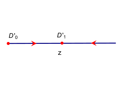
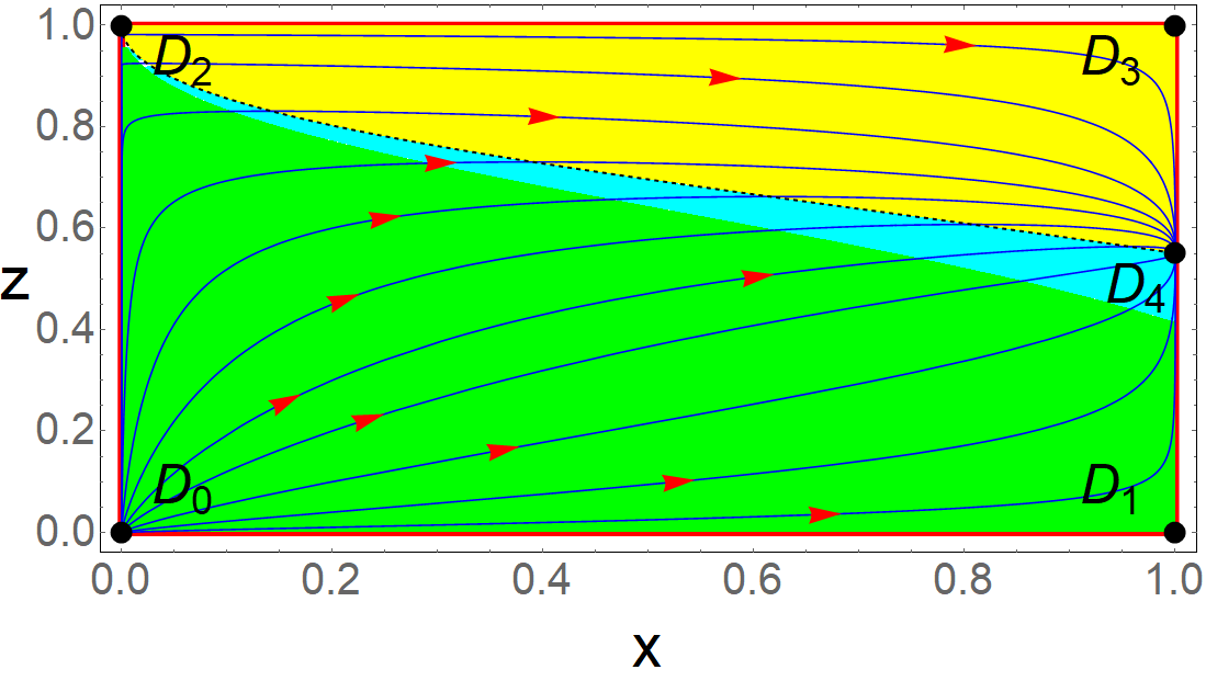
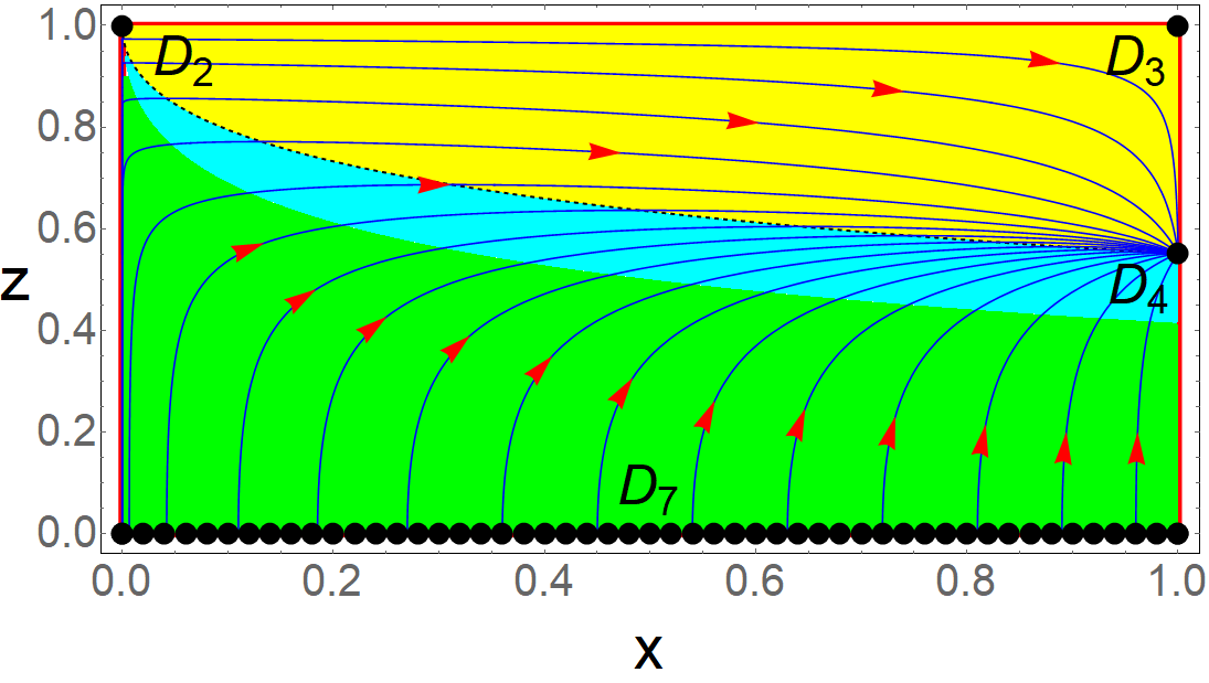
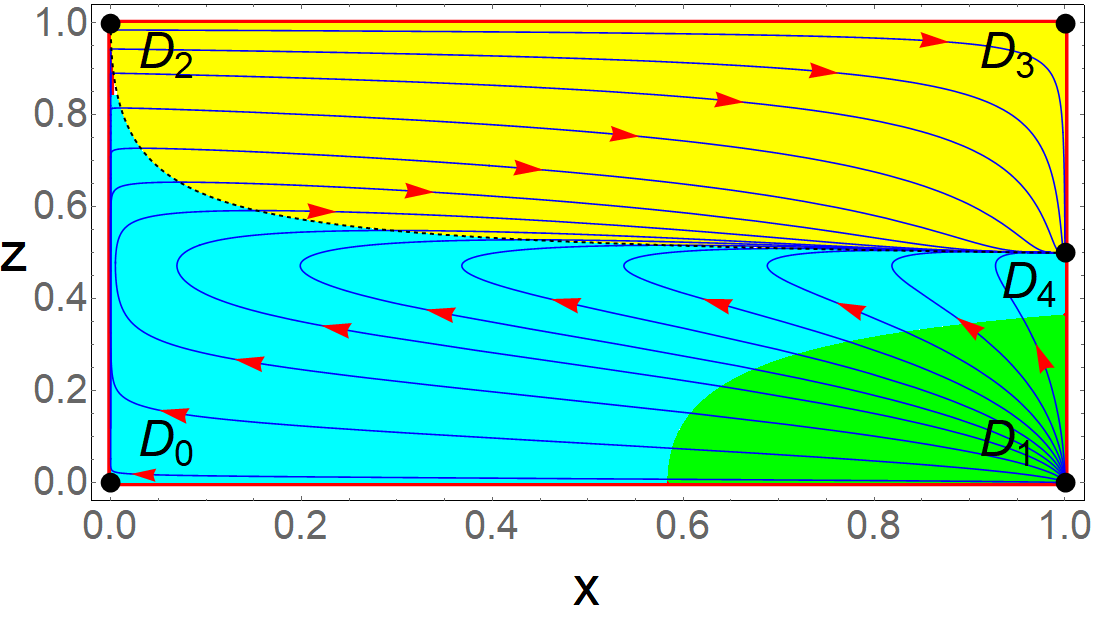
Figure 7: Description of the phase space controlled by the matter creation rate $\Gamma=\Gamma_{0}H^{-1}$, for both the one and two-fluid systems. Upper Left Plot: This is the vector plot of the one dimensional system (36) considering $\gamma=3$. However, for other positive values of $\gamma$, we can find similar type of plot. Upper Right Plot: The phase plot of the system (38) when we have assumed $w=1.5$ and $\gamma=2$. For other values of $w>0$ and $\gamma>0$, we can also obtain similar phase space structure. Lower Left Plot: The phase space of the system (38) when the equation of state $w$ takes the value $0$. Here we use $\gamma=2$ but any positive value of $\gamma$ gives same type of phase portrait. Lower Right Plot: The phase plot of the system (38) considering $w=-0.8$ and $\gamma=3$. Also, we can get similar type of graphics for any positive value of $\gamma$ and negative value of $w$ in the interval $(-1,0)$. Here the green region corresponds to the decelerating phase ($q>0$), the cyan region represents the accelerating phase with $-1<q<0$ and the yellow region corresponds to the super accelerating phase (i.e. $q<-1$). The black dotted curve separating the cyan and yellow regions corresponds to $q=-1$.

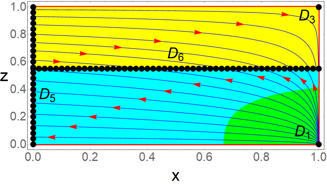
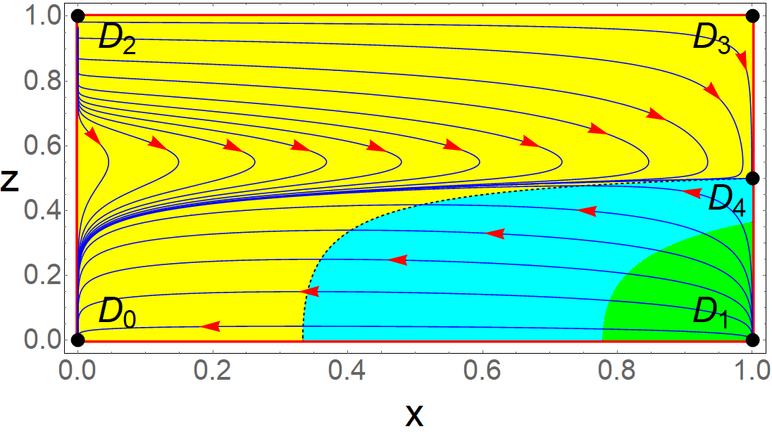
Figure 8: This figure also depicts the phase space of the two-fluid system driven by the matter creation rate $\Gamma=\Gamma_{0}H^{-1}$ but here we consider the case when $w\leq-1$. Left Plot: The phase space of the system (38) when the equation of state $w$ takes the value $-1$. Here we use $\gamma=2$ but any positive value of $\gamma$ gives similar type of phase portrait. Right Plot: The phase plot of the system (38) when we assume $w=-1.5$ and $\gamma=3$. For other values of $w<-1$ and $\gamma>0$, we can also obtain similar graphics. Here the green region corresponds to the decelerating phase ($q>0$), the cyan region represents the accelerating phase with $-1<q<0$ and the yellow region corresponds to the super accelerating phase (i.e. $q<-1$). The black dotted curve (in the left graph this curve is not visible because of the presence of the critical line) separating the cyan and yellow regions corresponds to $q=-1$.

1. When $w>0$: When the equation of state of the second fluid adopts positive values, we obtain five isolated critical points, namely, $D_{0},~D_{1},~D_{2},~D_{3}$ and $D_{4}$ in which $D_{0},~D_{2}$ are dominated by the second fluid only ($\Omega_{f}=1$) and $D_{1},~D_{3},~D_{4}$ are DM dominated points ($\Omega_{\rm dm}=1$). Inspecting the nature of eigenvalues from Table 4, according to the linear stability analysis, we find that $D_{0}$ is unstable, $D_{1},~D_{3}$ both are saddle by nature and $D_{4}$ is the only globally stable point. The critical point $D_{2}$ at which decelerating parameter is undefined, behaves like saddle point because along $z$ axis, $z$ is increasing and along $z=1$ line $x$ is increasing. Here, the points $D_{0},~D_{1}$ lie in the decelerating phase and $D_{3},D_{4}$ also belong to the accelerated phase of the universe. The phase space trajectories are highlighted in the upper right plot of the Fig. 7, indicating a transition of our universe from the second fluid dominated decelerating phase to a DM dominated accelerating phase where the slowing down of the cosmic acceleration is observed similar to what we have already seen for the two-fluid system of the Model $\Gamma=\Gamma_{0}$ with $w>0$, see section III.1.

2. When $w=0$: In this case, we obtain total three isolated critical points $D_{2},~D_{3},~D_{4}$ and one critical line $D_{7}(x_{c},0)$. In our phase space, $x^{\prime}$ is always positive and, $z$ is increasing for $z<\frac{1}{1+\sqrt{\frac{\gamma}{3}}\sqrt{x}}$ and it is decreasing for $z>\frac{1}{1+\sqrt{\frac{\gamma}{3}}\sqrt{x}}$. Therefore, $D_{7}$ where DM and DE coexist, is always unstable and $D_{2},~D_{3}$ give saddle type behavior. Since in our domain $D_{4}$ is the only stable point, we claim that it is a globally stable point. The accelerated phase includes $D_{3},~D_{4}$ and on the other side, the decelerated phase comprises the line $D_{7}$. The phase space orbits are depicted in the lower left plot of the Fig. 7, showing an alteration of the universe from the decelerating scaling solutions (DM and second fluid both exist in the picture) to DM dominated accelerating era where the slowing down of the cosmic acceleration is noted $-$ the same feature has been observed in the model $\Gamma=\Gamma_{0}$ with $w=0$, see section III.1.

3. When $-\frac{1}{3}\leq w<0$: In this interval of $w$, once again we can get five isolated critical points, namely, $D_{0},~D_{1},~D_{2},~D_{3}$ and $D_{4}$ by solving the autonomous system (38). Looking into the eigenvalues from the Table 3 and using the direction of the flow on the boundary of phase space, one can easily conclude about the stability of the critical points. Therefore, $D_{0},~D_{2}$ and $D_{3}$ give saddle type character, $D_{1}$ shows unstable nature and as before $D_{4}$ corresponds to matter dominated late time globally stable point. Here also, $D_{0}$, $D_{1}$ lie in the decelerating phase and $D_{3}$ belongs to the accelerating phase. The evolution of the solution curves are clearly observed in the lower right plot of the Fig. 7, highlighting the alteration from DM dominated decelerating epoch to DM dominated accelerating epoch with its slowing down nature, which one can meanwhile find in the Model III.1 with the case $-1/3<w<0$.

4. When $-1<w<-\frac{1}{3}$: This case properly replicates the above case where range of $w$ is $-\frac{1}{3}\leq w<0$. The only difference lie on the decelerating parameter at the point $D_{0}$ which shows acceleration. Thus the phase plot is the lower right plot of the Fig. 7.

5. When $w=-1$: Here, looking into the dynamical system (38), we can conclude that we have a set of critical points which contains two isolated critical points $D_{1},~D_{3}$ and two critical lines $D_{5}(0,z_{c})$, $D_{6}\left(x_{c},\frac{1}{1+\sqrt{\frac{\gamma}{3}}}\right)$. In the phase space above the line $z=\frac{1}{1+\sqrt{\frac{\gamma}{3}}}$, $x$ and $z$ show increasing and decreasing character, respectively, and below this line, $x$ is decreasing function while $z$ is increasing function. The equation of the separatrix joining the points $D_{1}$ and $\left(0,\frac{1}{\sqrt{\frac{\gamma}{3}}}\right)$ is $z=\sqrt{\frac{3}{\gamma}}(1-z)\sqrt{1-x}$ which separates the phase space below the line $z=\frac{1}{1+\sqrt{\frac{\gamma}{3}}}$ into two parts; one is below the separatrix and other one is the above the separatrix. In the first part, any trajectory approaches to the line $D_{5}$ and in the second part, trajectories converge to the line $D_{6}$. Therefore, $A_{6}$ where DM and DE coexist (except the end points), gives stable like nature. Here, $D_{1}$ and $D_{6}$ with $z>\frac{1}{1+\sqrt{\frac{\gamma}{3}}}$ show unstable nature and $D_{3}$ is a saddle point. The accelerating phase include $D_{3}$, $D_{5}$, $D_{6}$ and $D_{1}$ corresponds to deceleration. The part of the line $D_{5}$ below $z=\frac{1}{1+\sqrt{\frac{\gamma}{3}}}$ correspond to late time completely DE dominated stable points. On the other hand, the line $D_{6}$ has the ability to solve the coincidence problem. The phase space structure is properly presented in the left plot of the Fig. 8 which depicts two types of transitions: the first one is DM dominated decelerating phase to accelerating scaling solutions (DM and DE both exist) and the second one is DM dominated decelerating phase to completely DE dominated accelerating phase, that is similar to the case $w=-1$ of the Model III.1.

6. When $w<-1$: In the phantom region of $w$, we have again five critical points, namely, $D_{0},~D_{1},~D_{2},~D_{3},~D_{4}$ which lie on the boundary of the phase space region $R_{4}$. From the sign of the eigenvalues and the direction of the vector field on the boundary of the phase space, we can lead to the conclusion that $D_{1},~D_{2}$ are unstable critical points, $D_{3},~D_{4}$ give saddle type nature and $D_{0}$ is the only global stable critical point. Here, $D_{0},~D_{3},~D_{4}$ correspond to accelerating points and $D_{1}$ belong to deceleration phase. As a result $D_{1}$ is the past matter dominated unstable critical point and $D_{0}$ is the late time completely DE dominated late time stable critical point. The phase space orbits are exhibited in the right plot of Fig. 8, providing the transition from the DM dominated accelerating phase to the DE dominated super accelerating phase analogous to the case $w<-1$ of the Model III.1.

III.5 Model: $\Gamma=\Gamma_{0}H^{-2}$

In this series the last model is $\Gamma=\Gamma_{0}H^{-2}$ where $\Gamma_{0}$ is a constant with dimension equal to the dimension of the cube of the Hubble rate.

III.5.1 One fluid system

In the single fluid system, one dimensional autonomous system becomes,

$$z^{\prime}=\frac{3}{2}z\left(1-z-\frac{\mu z^{3}}{3(1-z)^{2}}\right),$$ (39)

which has the singularity at $z=1$ and $\mu=\frac{\Gamma_{0}}{H_{0}^{3}}$ is a parameter which always takes positive value. Removing this singularity by multiplying the positive factor $(1-z)^{2}$, the above system reduced to its regularized form:

$$z^{\prime}=\frac{3}{2}z\left((1-z)^{3}-\frac{\mu z^{3}}{3}\right).$$ (40)

Since, the decelerating parameter $q=\frac{1}{2}\left[1-\frac{\mu z^{3}}{(1-z)^{3}}\right]$ at present time (i.e. $z=1/2$) is $q=\frac{1-\mu}{2}$, hence, for the present time to have an accelerating phase of the universe, we should have $\mu>1$. This system has two critical points, namely $E^{\prime}_{0}$ and $E^{\prime}_{1}$ which are shown in Table 5. In $E^{\prime}_{0}$ and $E^{\prime}_{1}$, the first component corresponds to DM density parameter ($\Omega_{\rm dm}$), which always equals to $1$ and the second component stands for the $z$ variable. Both the critical points always represent matter dominated phase, but $E^{\prime}_{0}$ is an unstable point showing deceleration and $E^{\prime}_{1}$ gives acceleration with stable behavior. The stability behavior of the critical points are represented in the upper left plot of Fig. 9 by the direction of the vector field. The cosmological features are identical with the one-fluid system of the Models III.1 and III.4.

III.5.2 Two fluid system

The autonomous system in this case becomes,

$$x^{\prime}= x(1-x)\left(3w+\frac{\mu z^{3}}{(1-z)^{3}}\right),$$ (41a)

$$z^{\prime}= \frac{3}{2}z(1-z)\left[1+w(1-x)-\frac{\mu xz^{3}}{3(1-z)^{3}}\right],$$ (41b)

where $\mu=\frac{\Gamma_{0}}{H_{0}^{3}}$ is a dimensionless parameter adopting positive values. But as before, there is a singularity in the system at $z=1$ and we shall take aside this issue by regularization procedure using the positive factor $(1-z)^{3}$ and this leads to the following system

$$x^{\prime}= x(1-x)\left(3w(1-z)^{3}+\mu z^{3}\right),$$ (42a)

$$z^{\prime}= \frac{3}{2}z(1-z)\left[\left(1+w(1-x)\right)(1-z)^{3}-\frac{\mu xz^{3}}{3}\right].$$ (42b)

The Friedmann equation (11) and the dimensionless variables $x,~z$ defined in (24) gives our physical region which is again a unit square and we have named it as $R_{5}=[0,1]^{2}$. Here one can easily conclude that $R_{5}$ is a positively invariant set under the dynamical system (42) because boundaries of $R_{5}$ are invariant manifolds of (42). Here, $q=\frac{1}{2}\left[1+3w(1-x)-\frac{\mu xz^{3}}{(1-z)^{3}}\right]$. Therefore, at present time (i.e. $z=1/2$) for the accelerating expansion of the universe, the physical trajectories must follow the condition $(1-\mu)x+(1+3w)(1-x)<0$. The cosmological features that are obtained from the above system are briefly given in the Table 5. Now, we split the equation of state parameter in various parts and analyse the system (42) in each part of $w$, which have been described below:

		One fluid system
Critical point		Existence	Stability		$\Omega_{\rm dm}$	$q$	Acceleration
$E^{\prime}_{0}(1,0)$		Always	Always Unstable		1	$\frac{1}{2}$	No
$E^{\prime}_{1}\left(1,\frac{1}{1+\sqrt[3]{\frac{\mu}{3}}}\right)$		$\mu>0$	Always Stable		1	$-1$	Yes
		Two fluid system
Critical point	Existence	Eigenvalue	Stability	$\Omega_{f}$	$\Omega_{\rm dm}$	$q$	Acceleration
$E_{0}(0,0)$	Always	$\left(3w,\frac{3}{2}(1+w)\right)$	Stable if $w<-1$;	1	0	$\frac{1}{2}(1+3w)$	$w<-\frac{1}{3}$
			Saddle if $-1<w<0$;
			Unstable if $w>0$
$E_{1}(1,0)$	Always	$\left(-3w,\frac{3}{2}\right)$	Saddle if $w>0$;	0	1	$\frac{1}{2}$	No
			Unstable if $w<0$
$E_{2}(0,1)$	Always	$(\mu,0)$	Non-hyperbolic Saddle if $w>-1$;	1	0	Undefined	Undetermined
			Unstable if $w<-1$
$E_{3}(1,1)$	Always	$\left(-\mu,\frac{\mu}{2}\right)$	Always Saddle	0	1	$-\infty$	Yes
$E_{4}\left(1,\frac{1}{1+\sqrt[3]{\frac{\mu}{3}}}\right)$	$\mu>0$	$\left(-\frac{\mu(1+w)}{\left(1+\sqrt[3]{\frac{\mu}{3}}\right)^{3}},-\frac{3\mu}{2\left(1+\sqrt[3]{\frac{\mu}{3}}\right)^{3}}\right)$	Stable if $w>-1$	0	1	$-1$	Yes
			Saddle if $w<-1$
$E_{5}\left(0,z_{c}\right)$	$w=-1$	$\left(\mu z_{c}^{3}-3\left(1-z_{c}\right)^{3},0\right)$	Stable if $z_{c}<\frac{1}{1+\sqrt[3]{\frac{\mu}{3}}}$ and	$1$	$0$	$-1$	Yes
			Unstable if $z_{c}>\frac{1}{1+\sqrt[3]{\frac{\mu}{3}}}$
$E_{6}\left(x_{c},\frac{1}{1+\sqrt[3]{\frac{\mu}{3}}}\right)$	$w=-1$	$\left(0,-\frac{3\mu x_{c}}{2\left(1+\sqrt[3]{\frac{\mu}{3}}\right)^{3}}\right)$	Stable	$1-x_{c}$	$x_{c}$	$-1$	Yes
$E_{7}\left(x_{c},0\right)$	$w=0$	$\left(0,\frac{3}{2}\right)$	Unstable	$1-x_{c}$	$x_{c}$	$\frac{1}{2}$	No

Table 5: Summary of the critical points, their existence, stability and the values of the cosmological parameters at those points for the dynamical system (40) and (42) with the matter creation rate $\Gamma=\Gamma_{0}H^{-2}$.

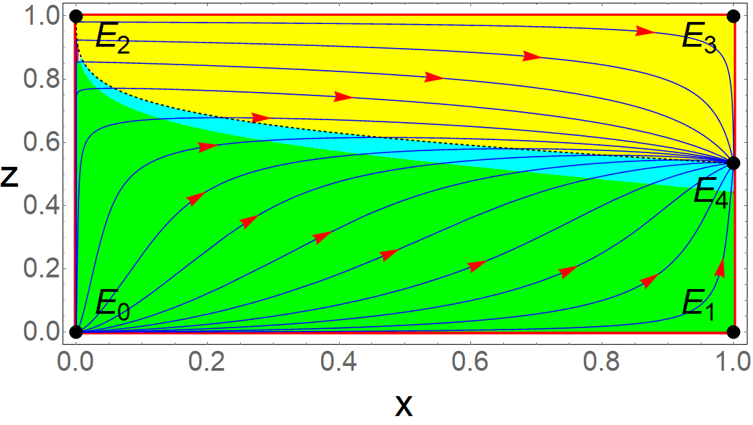
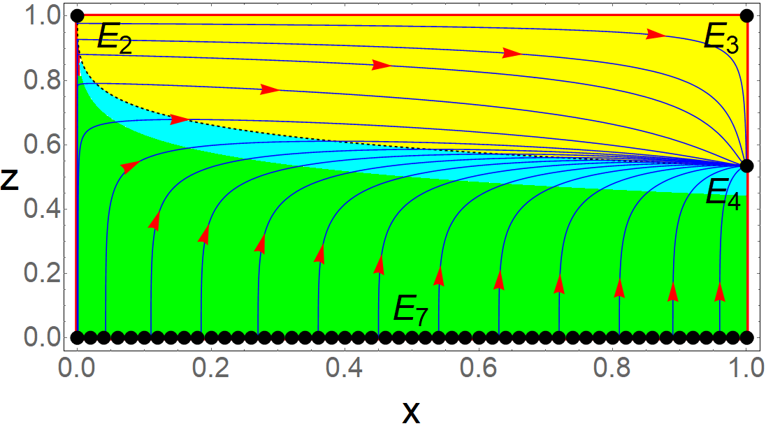
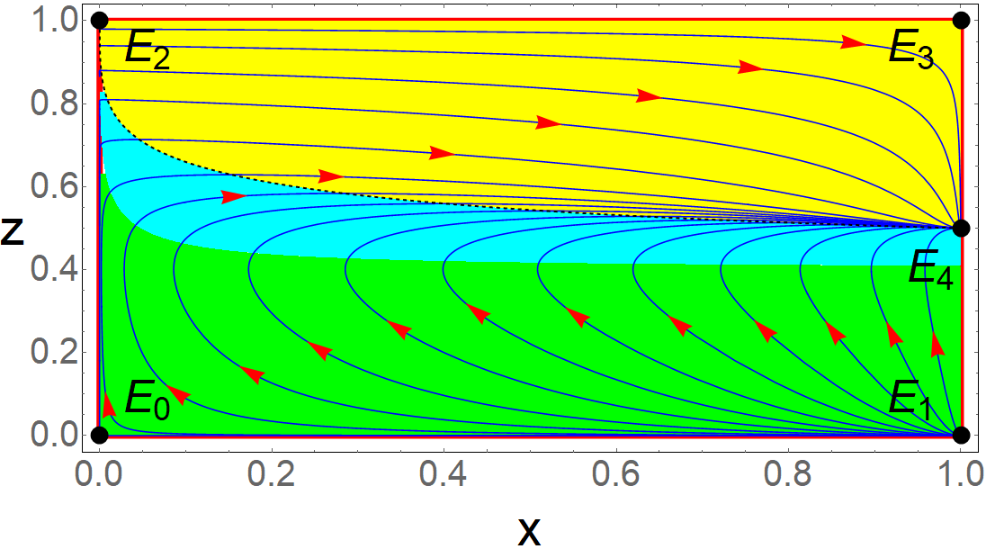
Figure 9: Description of the phase space structure of the one-fluid and two-fluid system for the matter creation rate $\Gamma=\Gamma_{0}H^{-2}$. Upper Left Plot: This is the vector plot of the one dimensional system (40) considering $\mu=3$. It is also noted that for other positive values of $\mu$, we can find similar type of plot. Upper Right Plot: The phase plot of the system (42) when we have assumed $w=0.5$ and $\mu=2$. For other values of $w>0$ and $\mu>0$, we can also obtain similar phase space structure. Lower Left Plot: The phase space of the system (42) when the equation of state $w$ takes the value $0$. Here we use $\mu=2$ but any positive value of $\mu$ gives same type of phase portrait. Lower Right Plot: The phase plot of the system (42) considering $w=-0.3$ and $\mu=3$. Also, we can get similar type of graphics for any positive value of $\mu$ and negative value of $w$ in the interval $(-1,0)$. Here the green region corresponds to the decelerating phase ($q>0$), the cyan region represents the accelerating phase with $-1<q<0$ and the yellow region corresponds to the super accelerating phase (i.e. $q<-1$). The black dotted curve separating the cyan and yellow regions corresponds to $q=-1$.

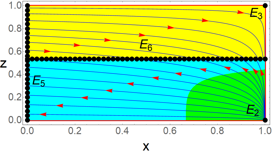
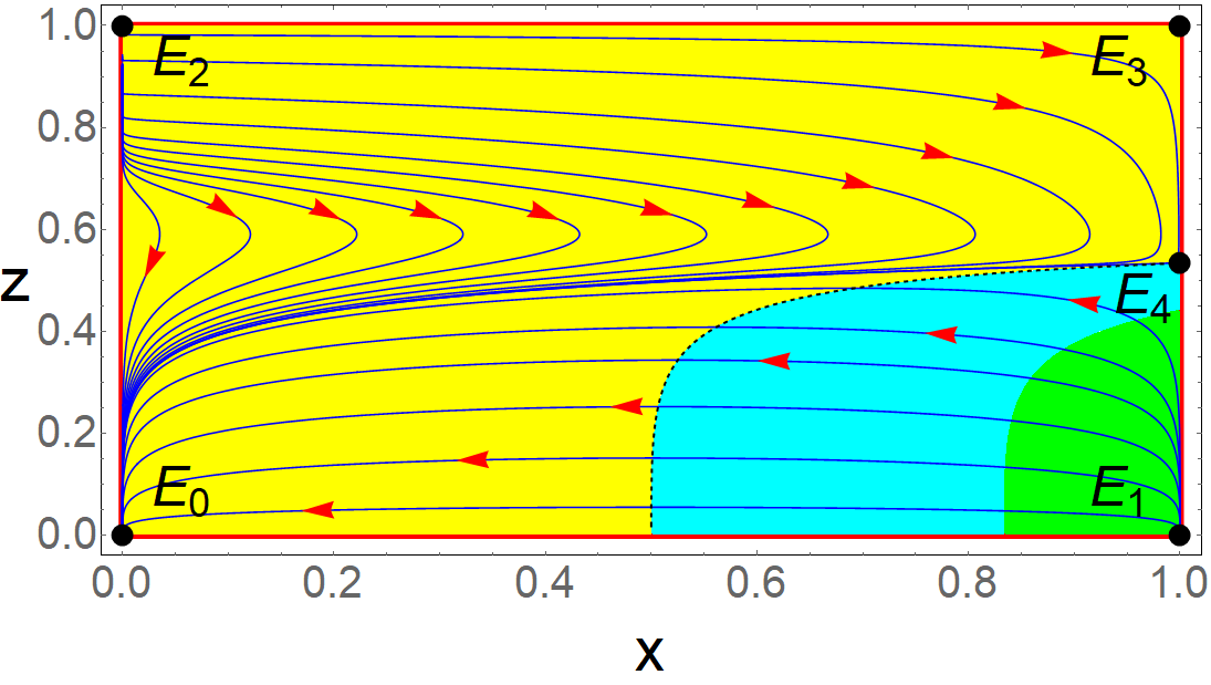
Figure 10: This figure depicts the phase space structure of the two-fluid system for the matter creation rate $\Gamma=\Gamma_{0}H^{-2}$ but here we consider the case when $w\leq-1$. Left Plot: The phase space of the system (42) when the equation of state $w$ takes the value $-1$. Here we use $\mu=2$ but any positive value of $\mu$ gives similar type of phase portrait. Right Plot: The phase plot of the system (42) when we assume $w=-2$ and $\mu=2$. For other values of $w<-1$ and $\mu>0$, we can also obtain similar graphics. Here the green region corresponds to the decelerating phase ($q>0$), the cyan region represents the accelerating phase with $-1<q<0$ and the yellow region corresponds to the super accelerating phase (i.e. $q<-1$). The black dotted curve separating the cyan and yellow regions (in the left graph this curve is not clear because of the critical line) corresponds to $q=-1$.

1. When $w>0$: For this part, the dynamical system (42) allows five critical points $E_{0},~E_{1},~E_{2},~E_{3}$ and $E_{4}$. Here, the accelerating phase includes the points $E_{3},~E_{4}$ and the decelerating phase contains the critical points $E_{0},~E_{1}$. Again, $E_{1},~E_{3},~E_{4}$ correspond to matter dominated solutions, while $E_{0},~E_{2}$ represent completely second fluid dominated points. One can easily conclude about stability from the direction of the vector field on the boundary of the phase space and signs of the eigenvalues. Therefore, $E_{0}$ is unstable, $E_{4}$ is the only globally stable point and $E_{1},~E_{2},~E_{3}$ are saddle by nature. Note that, $E_{4}$ is the DM dominated late time accelerating globally stable point. The upper right plot of Fig. 9 gives clear picture of the qualitative behavior of critical points. The inherent features of this plot are similar to the case $w>0$ of the Models III.1 and III.4.

2. When $w=0$: When the equation of state $w$ of the second fluid vanishes, we attain three isolated critical points $E_{2}(0,1),~E_{3}(1,1)$ and $E_{4}\left(1,\frac{1}{1+\sqrt[3]{\frac{\mu}{3}}}\right)$ along with one critical lines, namely, $E_{7}(x_{c},0)$. Now $x$ is always increasing and, $z$ is increasing and decreasing depending on $z$ variable chosen from $\left(0,\frac{1}{1+\sqrt[3]{\frac{\mu x}{3}}}\right)$ and $\left(\frac{1}{1+\sqrt[3]{\frac{\mu x}{3}}},1\right)$ respectively. Therefore $E_{2},~E_{3}$ are saddle, $E_{7}$ is unstable and $E_{4}$ is a globally stable critical point, which are obtained in the lower left plot of Fig. 9. Once again $E_{4}$ corresponds to DM dominated late time accelerated globally stable point. In this case, the cosmological characteristics are completely identical with the case $w=0$ of the Models III.1 and III.4.

3. When $-\frac{1}{3}\leq w<0$: Similar to the case where $w>0$, in this part of $w$, we acquire five isolated critical points which are depicted in the Table 5. From this table and the flow on the unit square, we can say that $E_{1}$ is unstable i.e. the DM dominated point $E_{1}$ leaves its decelerating phase, $E_{0},~E_{2},~E_{3}$ are saddle by behavior and once again, $E_{4}$ is the DM dominated accelerating globally stable point. Therefore, the universe ends with DM dominated accelerating phase. The orbits in the phase space are highlighted in the lower right plot of Fig. 9, providing the results which replicate the case $-1/3<w<0$ for the Models III.1 and III.4.

4. When $-1<w<-\frac{1}{3}$: This part of $w$ is analogous to the above case where $w$ lies in the interval $\left[-\frac{1}{3},0\right)$, except decelerating parameter at the critical point $E_{0}$ which belongs to the accelerating region in the phase space. Therefore, the phase plot is similar to the lower right plot of Fig. 9.

5. When $w=-1$: If the equation of state of non-matter creating fluid $w$ coincides with cosmological constant, we can obtain two isolated critical points $E_{1},~E_{3}$ which are mentioned in Table 5 and two critical lines, namely, $E_{5}(0,z_{c}),~E_{6}\left(x_{c},\frac{1}{1+\sqrt[3]{\frac{\mu}{3}}}\right)$. It is clear that $x^{\prime}$ is positive and negative respectively if we choose $z$ from the interval $\left(\frac{1}{1+\sqrt[3]{\frac{\mu}{3}}},1\right]$ and the interval $\left[0,\frac{1}{1+\sqrt[3]{\frac{\mu}{3}}}\right)$. Again $z$ is increasing and decreasing below and above the line $z=\frac{1}{1+\sqrt[3]{\frac{\mu}{3}}}$ respectively. In the phase space below the line $z=\frac{1}{1+\sqrt[3]{\frac{\mu}{3}}}$, the equation of the separatrix is $z=\sqrt[3]{\frac{3}{\mu}}(1-z)\sqrt{1-x}$ which connects the critical points $E_{1}$ and $\left(0,\frac{1}{1+\sqrt[3]{\frac{\mu}{3}}}\right)$. As a result, $E_{1}$ is unstable, $E_{3}$ is saddle, $E_{6}$ is stable and, $E_{5}$ is stable when $z_{c}<\frac{1}{1+\sqrt[3]{\frac{\mu}{3}}}$ and unstable when $z_{c}>\frac{1}{1+\sqrt[3]{\frac{\mu}{3}}}$. The left plot of Fig. 10 depicts qualitative features of the critical points. Here, $E_{5}$, lying in the accelerating phase, corresponds to completely DE domination and $E_{6}$, belonging also to the accelerating phase, represents the points where DM, DE coexist except the end points. Clearly, $E_{6}$ can solve cosmic coincidence problem. The key findings of this case are equivalent to the Models III.1 and III.4 with $w=-1$.

6. When $w<-1$: Here, one can get two unstable critical points $\left(E_{1},E_{2}\right)$, two saddle type critical points $\left(E_{3},E_{4}\right)$ and $E_{0}$ which is the only globally stable critical point. From Table 5, it is clear that, $E_{1}$ is the past decelerating DM dominated solution and point $E_{0}$ where the universe ends in the accelerating completely DE dominated phase. Also note that, $E_{3},~E_{4}$ lie in the accelerating phase and on the other hand, at $E_{2}$, acceleration can not be determined. The graphics in the right plot of Fig. 10 properly represents the stability character of the critical points, leading to the results which are very same as the case $w<-1$ for the Models III.1 and III.4.

	One-fluid system
Creation rate	Critical point	Existence	Stability	$\Omega_{dm}$	Acceleration
$\Gamma_{0}+\Gamma_{1}H$	$F^{\prime}_{1}(1,0)$	Always	Stable if $\beta\geq 3$ and Unstable if $\beta<3$	$1$	$q=(1-\beta)/2$, yes if $\beta>1$
	$F^{\prime}_{2}\left(1,\frac{3-\beta}{3-\beta+\alpha}\right)$	$\beta\leq 3$	Stable	$1$	$q=-1$, always yes
$\Gamma_{0}+\Gamma_{3}H^{-1}$	$G^{\prime}_{1}(1,0)$	Always	Unstable	$1$	$q=1/2$, no
	$G^{\prime}_{2}\left(1,\frac{6}{6+\alpha+\sqrt{\alpha^{2}+12\mu}}\right)$	Always	Stable	$1$	$q=-1$, always yes
$\Gamma_{0}+\Gamma_{2}H^{2}$	$I^{\prime}_{\pm}\left(1,\frac{3+2\gamma\pm\sqrt{9-4\alpha\gamma}}{2(3+\alpha+\gamma)}\right)$	$4\alpha\gamma\leq 9$	$I^{\prime}_{+}:$ Stable and $I^{\prime}_{-}:$ Unstable	$1$	$q=-1$, always yes
$\Gamma_{1}H+\Gamma_{2}H^{2}$	$J^{\prime}_{1}(1,1)$	Always	Unstable if $\beta\geq 3$ and Stable if $\beta<3$	$1$	$q=(1-\beta)/2$, yes if $\beta>1$
	$J^{\prime}_{2}\left(1,\frac{\gamma}{\gamma+3-\beta}\right)$	$\beta\leq 3$	Unstable	$1$	$q=-1$, always yes
$\Gamma_{1}H+\Gamma_{3}H^{-1}$	$L^{\prime}_{1}(1,0)$	Always	Unstable if $\beta<3$ and Stable if $\beta\geq 3$	$1$	$q=(1-\beta)/2$, yes if $\beta>1$
	$L^{\prime}_{2}\left(1,\frac{3-\beta-\sqrt{(3-\beta)\mu}}{3-\beta-\mu}\right)$	$\beta\leq 3,~\beta+\mu\neq 3$	Stable	$1$	$q=-1$, always yes
$\Gamma_{0}+\Gamma_{1}H+\Gamma_{2}H^{2}$	$M^{\prime}_{\pm}\left(1,\frac{3-\beta+2\gamma\pm\sqrt{(3-\beta)^{2}-4\alpha\gamma}}{2(3+\alpha-\beta+\gamma)}\right)$	$(3-\beta)^{2}-4\alpha\gamma\geq 0$,	$M^{\prime}_{+}:$ Stable	$1$	$q=-1$, always yes
		$3+2\alpha>\beta$,	and $M^{\prime}_{-}:$ Unstable
		$3+2\gamma>\beta$

Table 6: Properties of the critical points of the dynamical system (43), (47), (50), (53), (57) and (60) for the matter creation rate $\Gamma=\Gamma_{0}+\Gamma_{1}H,~\Gamma_{0}+\Gamma_{3}H^{-1},~\Gamma_{0}+\Gamma_{2}H^{2},~\Gamma_{1}H+\Gamma_{2}H^{2},~\Gamma_{1}H+\Gamma_{3}H^{-1}$ and $\Gamma_{0}+\Gamma_{1}H+\Gamma_{2}H^{2}$ respectively.

	Two-fluid system
Creation rate	Critical point	Existence	Stability	$\Omega_{dm}$	Acceleration
$\Gamma_{0}+\Gamma_{1}H$	$F_{0}(0,0)$	Always	Stable if $3w+\beta<0,~w<-1$;	$0$	Yes if $w<-1$
	$F_{1}(1,0)$	Always	Stable if $3w+\beta>0,~\beta\geq 3$;	$1$	Yes if $\beta>1$
	$F_{2}(0,1)$	Always	Unstable	$0$	Undetermined
	$F_{3}(1,1)$	Always	Always Saddle	$1$	Always yes
	$F_{4}\left(1,\frac{3-\beta}{3-\beta+\alpha}\right)$	$\beta\leq 3$	Stable if $w>-1$	$1$	Always yes
	$F_{5}\left(0,z_{c}\right)$	$w=-1$	Stable if $\beta-3+(3-\beta+\alpha)z_{c}>0$	$0$	Always yes
	$F_{6}\left(x_{c},\frac{3-\beta}{3-\beta+\alpha}\right)$	$w=-1,~\beta\leq 3$	Always Stable	$x_{c}$	Always yes
	$F_{7}\left(x_{c},0\right)$	$3w+\beta=0$	Stable if $w<-1$	$x_{c}$	Yes if $\beta>1$
$\Gamma_{0}+\Gamma_{3}H^{-1}$	$G_{0}(0,0)$	Always	Stable if $w<-1$;	$0$	Yes if $w<-\frac{1}{3}$
	$G_{1}(1,0)$	Always	Saddle if $w>0$, Unstable if $w<0$;	$1$	No
	$G_{2}(0,1)$	Always	Unstable/Saddle	$0$	Undetermined
	$G_{3}(1,1)$	Always	Saddle	$1$	Always yes
	$G_{4}\left(1,\frac{6}{6+\alpha+\sqrt{\alpha^{2}+12\mu}}\right)$	Always	Always Stable	$1$	Always yes
	$G_{5}\left(x_{c},0\right)$	$w=0$	Unstable	$x_{c}$	No
	$G_{6}\left(x_{c},\frac{6}{6+\alpha+\sqrt{\alpha^{2}+12\mu}}\right)$	$w=-1$	Always Stable	$x_{c}$	Always yes
	$G_{7}\left(0,z_{c}\right)$	$w=-1$	Stable if $z_{c}>(<)\frac{6}{6+\alpha+\sqrt{\alpha^{2}+12\mu}}$, $3+\alpha-\mu>(<)0$;	$0$	Always yes
			Unstable if $z_{c}<(>)\frac{6}{6+\alpha+\sqrt{\alpha^{2}+12\mu}}$, $3+\alpha-\mu>(<)0$
$\Gamma_{0}+\Gamma_{2}H^{2}$	$I_{0}(0,0)$	Always	Unstable/Saddle	$0$	Undetermined
	$I_{1}(1,0)$	Always	Always Stable	$1$	Always yes
	$I_{2}(0,1)$	Always	Unstable/Saddle	$0$	Undetermined
	$I_{3}(1,1)$	Always	Saddle	$1$	Always yes
	$I_{4\pm}\left(1,\frac{3+2\gamma\pm\sqrt{9-4\alpha\gamma}}{2(3+\alpha+\gamma)}\right)$	$4\alpha\gamma\leq 9$	$I_{4+}:$ Stable if $w>-1$, otherwise Saddle	$1$	Always yes
			$I_{4-}:$ Unstable/Saddle
	$I_{5\pm}\left(x_{c},\frac{3+2\gamma\pm\sqrt{9-4\alpha\gamma}}{2(3+\alpha+\gamma)}\right)$	$4\alpha\gamma\leq 9,~w=-1$	$I_{5+}:$ Stable; $I_{5-}:$ Unstable	$x_{c}$	Always yes
	$I_{6}\left(0,z_{c}\right)$	$w=-1$	Stable if $\frac{3+2\gamma-\sqrt{9-4\alpha\gamma}}{2(3+\alpha+\gamma)}<z_{c}<\frac{3+2\gamma+\sqrt{9-4\alpha\gamma}}{2(3+\alpha+\gamma)}$	$0$	Always yes
			Unstable if $z_{c}<\frac{3+2\gamma-\sqrt{9-4\alpha\gamma}}{2(3+\alpha+\gamma)}$ or $z_{c}>\frac{3+2\gamma-\sqrt{9-4\alpha\gamma}}{2(3+\alpha+\gamma)}$

Table 7: Properties of the critical points of the dynamical system (45), (49) and (52) for the matter creation rate $\Gamma=\Gamma_{0}+\Gamma_{1}H$, $\Gamma_{0}+\Gamma_{3}H^{-1}$ and $\Gamma_{0}+\Gamma_{2}H^{2}$ respectively.

	Two-fluid system
Creation rate	Critical point	Existence	Stability	$\Omega_{dm}$	Acceleration
$\Gamma_{1}H+\Gamma_{2}H^{2}$	$J_{0}(0,0)$	Always	Unstable/Saddle	$0$	Undetermined
	$J_{1}(1,0)$	Always	Always Stable	$1$	Always yes
	$J_{2}(0,1)$	Always	Stable if $w\leq-\frac{\beta}{3}$, $w>-1$	$0$	Yes if $w<-\frac{1}{3}$
	$J_{3}(1,1)$	Always	Stable if $w>-\frac{\beta}{3}$, $\beta<3$	$1$	Yes if $\beta>1$
	$J_{4}\left(1,\frac{\gamma}{\gamma+3-\beta}\right)$	$\beta\leq 3$	Saddle if $w>-1$; Unstable if $w<-1$	$1$	Always yes
	$J_{5}\left(x_{c},\frac{\gamma}{\gamma+3-\beta}\right)$	$w=-1,~\beta\leq 3$	Unstable	$x_{c}$	Always yes
	$J_{6}\left(0,z_{c}\right)$	$w=-1$	Stable if $\gamma-(\gamma+3-\beta)z_{c}<0$	$0$	Always yes
	$J_{7}\left(x_{c},1\right)$	$\beta+3w=0$	Stable if $\beta<3$	$x_{c}$	Yes if $\beta>1$
$\Gamma_{1}H+\Gamma_{3}H^{-1}$	$L_{0}(0,0)$	Always	Stable if $w\leq-\frac{\beta}{3},~w<-1$	$0$	Yes if $w<-\frac{1}{3}$
	$L_{1}(1,0)$	Always	Stable if $w>-\frac{\beta}{3},~\beta\geq 3$	$1$	Yes if $\beta>1$
	$L_{2}(0,1)$	Always	Unstable/Saddle	$0$	Undetermined
	$L_{3}(1,1)$	Always	Saddle	$1$	Always yes
	$L_{4}\left(1,\frac{3-\beta-\sqrt{(3-\beta)\mu}}{3-\beta-\mu}\right)$	$\beta\leq 3$	Stable if $w>-1,~\beta+\mu\neq 3$	$1$	Always yes
	$L_{5}\left(x_{c},\frac{3-\beta-\sqrt{(3-\beta)\mu}}{3-\beta-\mu}\right)$	$w=-1,~\beta\leq 3$	Stable if $\beta<3,~\beta+\mu\neq 3$	$x_{c}$	Always yes
	$L_{6}\left(0,z_{c}\right)$	$w=-1$	Stable if $z_{c}<\frac{3-\beta-\sqrt{(3-\beta)\mu}}{3-\beta-\mu}$; Unstable if $z_{c}>\frac{3-\beta-\sqrt{(3-\beta)\mu}}{3-\beta-\mu}$	$0$	Always yes
	$L_{7}\left(x_{c},0\right)$	$\beta+3w=0$	Stable if $\beta>3$	$x_{c}$	Yes if $\beta>1$
$\Gamma_{0}+\Gamma_{1}H+\Gamma_{2}H^{2}$	$M_{0}(0,0)$	Always	Unstable/Saddle	$0$	Undetermined
	$M_{1}(1,0)$	Always	Always Stable	$1$	Always yes
	$M_{2}(0,1)$	Always	Unstable/Saddle	$0$	Undetermined
	$M_{3}(1,1)$	Always	Saddle	$1$	Always yes
	$M_{4\pm}\left(1,\frac{3-\beta+2\gamma\pm\sqrt{(3-\beta)^{2}-4\alpha\gamma}}{2(3+\alpha-\beta+\gamma)}\right)$	$(3-\beta)^{2}-4\alpha\gamma\geq 0$,	$M_{4+}:$ Stable if $w>-1$, Saddle if $w<-1$	$1$	Always yes
		$3+2\alpha>\beta,~3+2\gamma>\beta$;	$M_{4-}:$ Unstable if $w<-1$, Saddle if $w>-1$
	$M_{5\pm}\left(x_{c},\frac{3-\beta+2\gamma\pm\sqrt{(3-\beta)^{2}-4\alpha\gamma}}{2(3+\alpha-\beta+\gamma)}\right)$	$(3-\beta)^{2}-4\alpha\gamma\geq 0,~w=-1$,	$M_{5+}:$ Stable; $M_{5-}:$ Unstable	$x_{c}$	Always yes
		$3+2\alpha>\beta,~3+2\gamma>\beta$;
	$M_{6}\left(0,z_{c}\right)$	$w=-1$	Stable if $\frac{3-\beta+2\gamma-\sqrt{(3-\beta)^{2}-4\alpha\gamma}}{2(3+\alpha-\beta+\gamma)}<z_{c}<\frac{3-\beta+2\gamma+\sqrt{(3-\beta)^{2}-4\alpha\gamma}}{2(3+\alpha-\beta+\gamma)}$,	$0$	Always yes
			$(3-\beta)^{2}-4\alpha\gamma\geq 0,~3+2\alpha>\beta,~3+2\gamma>\beta$;
			Unstable if $z_{c}<\frac{3-\beta+2\gamma-\sqrt{(3-\beta)^{2}-4\alpha\gamma}}{2(3+\alpha-\beta+\gamma)}$ or $z_{c}>\frac{3-\beta+2\gamma+\sqrt{(3-\beta)^{2}-4\alpha\gamma}}{2(3+\alpha-\beta+\gamma)}$,
			$(3-\beta)^{2}-4\alpha\gamma\geq 0,~3+2\alpha>\beta,~3+2\gamma>\beta$;

Table 8: Properties of the critical points of the dynamical system (55), (59) and (62) for the matter creation rate $\Gamma=\Gamma_{1}H+\Gamma_{2}H^{2}$, $\Gamma_{1}H+\Gamma_{3}H^{-1}$ and $\Gamma_{0}+\Gamma_{1}H+\Gamma_{2}H^{2}$ respectively.

III.6 Model: $\Gamma=\Gamma_{0}+\Gamma_{1}H$

We start with the matter creation model $\Gamma=\Gamma_{0}+\Gamma_{1}H$ which has two free parameters, namely, $\Gamma_{0}$ and $\Gamma_{1}$, and this model represents the linear combination of the matter creation models, namely, $\Gamma=\Gamma_{0}$ and $\Gamma\propto H$. For this model, the dynamics within the one fluid system is described by

$$z^{\prime}=\frac{1}{2}z\left[(3-\beta)(1-z)-\alpha z\right],$$ (43)

where $\alpha~(=\Gamma_{0}/H_{0})$ and $\beta~(=\Gamma_{1})$ are two dimensionless positive constants. In Table 6 we present the critical points and their nature. It is also noted that the results are already seen in the Model III.1 ($\Gamma=\Gamma_{0}$) and III.2 ($\Gamma=\Gamma_{0}H$) for one fluid system.

On the other hand, for the two-fluid system, the autonomous system reads

$$x^{\prime}= x(1-x)\left[3w+\frac{\alpha z}{1-z}+\beta\right],$$ (44a)

$$z^{\prime}= \frac{3}{2}z(1-z)\left[1+w(1-x)-\frac{x}{3}\left(\frac{\alpha z}{1-z}+\beta\right)\right],$$ (44b)

in which $\alpha~(=\Gamma_{0}/H_{0})$ and $\beta~(=\Gamma_{1})$ are the dimensionless positive parameters and after regularization, eqn. (44) becomes

$$x^{\prime}= x(1-x)\left[3w(1-z)+\alpha z+\beta(1-z)\right],$$ (45a)

$$z^{\prime}= \frac{3}{2}z(1-z)\Big{[}\left(1+w(1-x)\right)(1-z)$$

$$-\frac{x}{3}\left(\alpha z+\beta(1-z)\right)\Big{]}.$$ (45b)

In Table 7 we present the critical points for this model and their nature. The critical line $F_{7}$ where both the fluid share energy density, giving stable qualitative nature in the phantom region $(w<-1)$, represents acceleration if we choose $\beta>1$. Thus, there is a possibility to reduce the coincidence problem in the phantom region otherwise this model can offer the results which we have noticed for the Model III.1 ($\Gamma=\Gamma_{0}$) and III.2 ($\Gamma=\Gamma_{0}H$).

III.7 Model: $\Gamma=\Gamma_{0}+\Gamma_{3}H^{-1}$

We consider the second model in this series as $\Gamma=\Gamma_{0}+\Gamma_{3}H^{-1}$ having two parameters $\Gamma_{0}$ and $\Gamma_{3}$ and this model presents the linear combination of the models $\Gamma=\Gamma_{0}$ and $\Gamma\propto H^{-1}$. For the single fluid system, the dynamics of the model can be described by

$$z^{\prime}=\frac{3}{2}z\left[1-z-\frac{z(\alpha(1-z)+\mu z)}{3(1-z)}\right],$$ (46)

where $\alpha~(=\Gamma_{0}/H_{0}),~\mu~(=\Gamma_{3}/H_{0}^{2})$ are the dimensionless positive free parameters. However, this equation admits a singularity at $z=1$, hence, we regularize this system and it becomes,

$$z^{\prime}=\frac{3}{2}z\left[(1-z)^{2}-\frac{z(\alpha(1-z)+\mu z)}{3}\right].$$ (47)

In Table 6 we present the results in terms of the critical points and their stability. These results are completely identical with the Models III.1 ($\Gamma=\Gamma_{0}$), III.4 ($\Gamma=\Gamma_{0}H^{-1}$) and III.5 ($\Gamma=\Gamma_{0}H^{-2}$).

For the two-fluid system, the autonomous system reads

$$x^{\prime}= x(1-x)\left[3w+\frac{\alpha z(1-z)+\mu z^{2}}{(1-z)^{2}}\right],$$ (48a)

$$z^{\prime}= \frac{3}{2}z(1-z)\Big{[}1+w(1-x)$$

$$-\frac{x}{3}\left(\frac{\alpha z(1-z)+\mu z^{2}}{(1-z)^{2}}\right)\Big{]},$$ (48b)

where $\alpha~(=\Gamma_{0}/H_{0}),~\mu~(=\Gamma_{3}/H_{0}^{2})$ are the dimensionless positive free parameters. Similarly, this system admits a singularity at $z=1$. Thus, we regularize this system and after regularization, the system becomes,

$$x^{\prime}= x(1-x)\left[3w(1-z)^{2}+\alpha z(1-z)+\mu z^{2}\right],$$ (49a)

$$z^{\prime}= \frac{3}{2}z(1-z)\Big{[}\left(1+w(1-x)\right)(1-z)^{2}$$

$$-\frac{x}{3}\left(\alpha z(1-z)+\mu z^{2}\right)\Big{]}.$$ (49b)

In Table 7 we present the critical points and their corresponding analysis. Here, also cosmological implications are similar to the Models III.1 ($\Gamma=\Gamma_{0}$), III.4 ($\Gamma=\Gamma_{0}H^{-1}$) and III.5 ($\Gamma=\Gamma_{0}H^{-2}$).

III.8 Model: $\Gamma=\Gamma_{0}+\Gamma_{2}H^{2}$

We now consider the following model $\Gamma=\Gamma_{0}+\Gamma_{2}H^{2}$ with $\Gamma_{0}$ and $\Gamma_{2}$ as two free parameters. For the one fluid system, the dynamics of the model is described by

$$z^{\prime}=\frac{3}{2}\left[z(1-z)-\frac{\left(\alpha z^{2}+\gamma(1-z)^{2}\right)}{3}\right],$$ (50)

where we have introduced two dimensionless positive parameters, namely, $\alpha~(=\Gamma_{0}/H_{0})$ and $\gamma~(=\Gamma_{2}H_{0})$. Note that the above equation does not admit any singularity for any $z$. In Table 6 we present the results. These results are analogous to the results which the Model III.2 can offer.

For the two-fluid system, we get the following autonomous system

$$x^{\prime}= x(1-x)\left[3w+\frac{\alpha z^{2}+\gamma(1-z)^{2}}{z(1-z)}\right],$$ (51a)

$$z^{\prime}= \frac{3}{2}z(1-z)\Big{[}1+w(1-x)-\frac{x}{3}\left(\frac{\alpha z^{2}+\gamma(1-z)^{2}}{z(1-z)}\right)\Big{]},$$ (51b)

where $\alpha~(=\Gamma_{0}/H_{0})$ and $\gamma~(=\Gamma_{2}H_{0})$ are the dimensionless positive parameters. Notice that the system (51) has singularities at $z=0$ and $z=1$. We regularize the system (51) and this now reads

$$x^{\prime}= x(1-x)\left[3wz(1-z)+\alpha z^{2}+\gamma(1-z)^{2}\right],$$ (52a)

$$z^{\prime}= \frac{3}{2}z(1-z)\Big{[}\left(1+w(1-x)\right)z(1-z)$$

$$-\frac{x}{3}\left(\alpha z^{2}+\gamma(1-z)^{2}\right)\Big{]}.$$ (52b)

In Table 7 we present the results. The cosmological features are previously found in the Models III.1 ($\Gamma=\Gamma_{0}$) and III.3 ($\Gamma=\Gamma_{0}H^{2}$).

III.9 Model: $\Gamma=\Gamma_{1}H+\Gamma_{2}H^{2}$

We now consider the linear combination of the models $\Gamma\propto H$ and $\Gamma\propto H^{2}$, that means, $\Gamma=\Gamma_{1}H+\Gamma_{2}H^{2}$ where $\Gamma_{1}$ and $\Gamma_{2}$ are constants. For the one fluid system, the dynamics of the model is described by the following equation

$$z^{\prime}=\frac{3}{2}(1-z)\left[z-\frac{\left(\beta z+\gamma(1-z)\right)}{3}\right],$$ (53)

where $\beta=\Gamma_{1}$, $\gamma=\Gamma_{2}H_{0}$ are the dimensionless positive constants and the above equation has no singularity. The critical points and their nature are presented in Table 6. For this model, one can recover the results from the Models III.2 ($\Gamma=\Gamma_{0}H$) and III.3 ($\Gamma=\Gamma_{0}H^{2}$).

We now proceed to the two-fluid system for which the autonomous system reads

$$x^{\prime}= x(1-x)\left[3w+\frac{\beta z+\gamma(1-z)}{z}\right],$$ (54a)

$$z^{\prime}= \frac{3}{2}z(1-z)\Big{[}1+w(1-x)-\frac{x}{3}\left(\frac{\beta z+\gamma(1-z)}{z}\right)\Big{]},$$ (54b)

where $\beta=\Gamma_{1}$, $\gamma=\Gamma_{2}H_{0}$ are the dimensionless positive constants, and this system admits a singularity at $z=0$. After regularizing the system (54b) one arrives at

$$x^{\prime}= x(1-x)\left[3wz+\beta z+\gamma(1-z)\right],$$ (55a)

$$z^{\prime}= \frac{3}{2}z(1-z)\Big{[}\left(1+w(1-x)\right)z-\frac{x}{3}\left(\beta z+\gamma(1-z)\right)\Big{]}.$$ (55b)

We perform the phase space analysis for this system and in Table 8 we present the results. One can notice that the critical line $J_{7}$ alleviates cosmic coincidence problem for $-1<w<-\frac{1}{3}$ and the other consequences of this creation rate can be recovered from the Models III.2 ($\Gamma=\Gamma_{0}H$) and III.3 ($\Gamma=\Gamma_{0}H^{2}$).

III.10 Model: $\Gamma=\Gamma_{1}H+\Gamma_{3}H^{-1}$

Considering the linear combinations of the models, namely, $\Gamma\propto H$ and $\Gamma\propto H^{-1}$, we consider the following model $\Gamma=\Gamma_{1}H+\Gamma_{3}H^{-1}$ in which $\Gamma_{1}$ and $\Gamma_{3}$ are constants. The dynamics for the one fluid system is described by the following equation

$$z^{\prime}=\frac{3}{2}z\left[1-z-\frac{\left(\beta(1-z)^{2}+\mu z^{2}\right)}{3(1-z)}\right],$$ (56)

where $\beta~(=\Gamma_{1})$ and $\mu~(=\Gamma_{3}/H_{0}^{2})$ are dimensionless positive constants. We notice that the above equation has a singularity at $z=1$, thus, we regularize this one dimensional system leading to

$$z^{\prime}=\frac{3}{2}z\left[(1-z)^{2}-\frac{\left(\beta(1-z)^{2}+\mu z^{2}\right)}{3}\right].$$ (57)

In Table 6 we present the critical points and their stability. The different characteristics of the critical points can be observed from the Models III.2 ($\Gamma=\Gamma_{0}H$) and III.4 ($\Gamma=\Gamma_{0}H^{-1}$).

For the two-fluid system, we have the following autonomous system

$$x^{\prime}= x(1-x)\left[3w+\beta+\frac{\mu z^{2}}{(1-z)^{2}}\right],$$ (58a)

$$z^{\prime}= \frac{3}{2}z(1-z)\Big{[}1+w(1-x)-\frac{x}{3}\left(\beta+\frac{\mu z^{2}}{(1-z)^{2}}\right)\Big{]},$$ (58b)

where $\beta=\Gamma_{1}$ and $\mu=\Gamma_{3}/H_{0}^{2}$ are the dimensionless positive parameters. Notice that the system (58) has a singularity at $z=1$. We regularize the system (58) which finally reduces to

$$x^{\prime}= x(1-x)\left[(3w+\beta)(1-z)^{2}+\mu z^{2}\right],$$ (59a)

$$z^{\prime}= \frac{3}{2}z(1-z)\Big{[}\left(1+w(1-x)\right)(1-z)^{2}$$

$$-\frac{x}{3}\left(\beta(1-z)^{2}+\mu z^{2}\right)\Big{]}.$$ (59b)

In Table 8 we present the critical points and their stability. Here, in the phantom region $(w<-1)$, the critical point $L_{7}$ is a candidate of solving cosmic coincidence problem, otherwise the results which this model can offer, are already presented in the Models III.2 ($\Gamma=\Gamma_{0}H$) and III.4 ($\Gamma=\Gamma_{0}H^{-1}$).

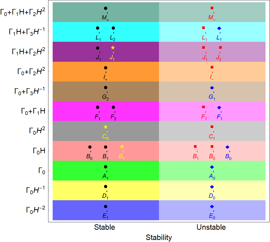
Figure 11: This is the summary diagram for the one-fluid system in terms of qualitative behavior of the critical points, i.e. unstable (solid square and diamond) and stable (solid circle and five-star). Here, the black solid circles (or the yellow solid five-stars) represent late-time accelerating (decelerating) solutions and the blue solid diamonds (or the red solid squares) indicate decelerating (accelerating) solutions.

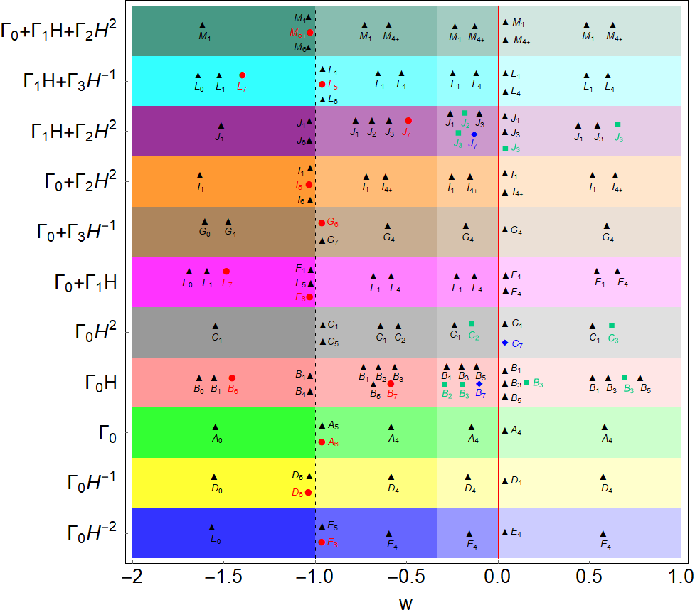
Figure 12: This is a summary picture for the two-fluid matter creating scenarios in terms of various critical points obtained for different regions of $w$. The critical points leading to accelerating attractors at late-time (black solid triangles), accelerating scaling attractors at late-time (red solid circles), decelerating attractors (green solid squares) and decelerating scaling attractors (blue solid diamonds) are displayed. The vertical solid red line corresponds to $w=0$ and the vertical black dashed line corresponds to $w=-1$. The figure emphasizes that all models admit accelerating attractors at late-time for $w\geq 0$, that means without any need of hypothetical fluid with negative pressure. It is also notable that some models can produce decelerating attractors for $w\geq-\frac{1}{3}$, that means our universe may enter in the decelerating phase and remain in this phase, while for $w<-\frac{1}{3}$, all the models can provide late-time accelerating attractors which may be DE dominated, scaling solutions (DE and DM both exist) or DM dominated.

III.11 Model: $\Gamma=\Gamma_{0}+\Gamma_{1}H+\Gamma_{2}H^{2}$

We now consider a three parameter matter creation model of the form $\Gamma=\Gamma_{0}+\Gamma_{1}H+\Gamma_{2}H^{2}$ where $\Gamma_{0}$, $\Gamma_{1}$ and $\Gamma_{2}$ are constants. For the one fluid system, the dynamics of the model can be described by the following one dimensional system

$$z^{\prime}=\frac{3}{2}\left[z(1-z)-\left(\frac{\alpha z^{2}+\beta z(1-z)+\gamma(1-z)^{2}}{3}\right)\right],$$ (60)

where $\alpha~(=\Gamma_{0}/H_{0}),~\beta~(=\Gamma_{1})$, $\gamma=\Gamma_{2}H_{0}$, are the dimensionless positive constants. Note that the above equation does not admit any singularity for any $z$. We perform the phase space analysis for this system and in Table 6 we present the critical points and their behavior. The Models III.1 ($\Gamma=\Gamma_{0}$), III.2 ($\Gamma=\Gamma_{0}H$) and III.3 ($\Gamma=\Gamma_{0}H^{2}$) also deliver the results which we have found in this context.

For the two fluid system, the autonomous system becomes,

$$x^{\prime}= x(1-x)\left[3w+\frac{\alpha z^{2}+\beta z(1-z)+\gamma(1-z)^{2}}{z(1-z)}\right],$$ (61a)

$$z^{\prime}= \frac{3}{2}z(1-z)\Big{[}1+w(1-x)$$

$$-\frac{x}{3}\left(\frac{\alpha z^{2}+\beta z(1-z)+\gamma(1-z)^{2}}{z(1-z)}\right)\Big{]},$$ (61b)

where $\alpha~(=\Gamma_{0}/H_{0}),~\beta~(=\Gamma_{1})$, $\gamma=\Gamma_{2}H_{0}$, are the dimensionless positive constants, however, the above system has two singularities, one at $z=0$ and the other at $z=1$. We regularize the system (61) and the final system reads

$$x^{\prime}= x(1-x)\Big{[}3wz(1-z)+\alpha z^{2}$$

$$+\beta z(1-z)+\gamma(1-z)^{2}\Big{]},$$ (62a)

$$z^{\prime}= \frac{3}{2}z(1-z)\Big{[}(1+w(1-x))z(1-z)$$

$$-\frac{x}{3}\left(\alpha z^{2}+\beta z(1-z)+\gamma(1-z)^{2}\right)\Big{]}.$$ (62b)

We perform the phase space analysis and in Table 8 we present the corresponding results. The cosmological results are not new in this context. Meanwhile, we have obtained this results for the Models III.1 ($\Gamma=\Gamma_{0}$), III.2 ($\Gamma=\Gamma_{0}H$) and III.3 ($\Gamma=\Gamma_{0}H^{2}$).

IV Summary and Conclusions

CCDM cosmology was proposed as an alternative to the DE and MG theories and because of this elegant nature, this came to the limelight of modern cosmology. In this article we have studied CCDM cosmologies by applying the powerful technique of dynamical analysis aiming to closely examine whether such cosmological scenarios can predict various phases of our universe’s evolution. We have considered two distinct cosmological scenarios, namely, a single fluid system consisting of a pressure-less DM endowed with matter production, and a two-fluid system consisting of a pressure-less DM responsible for the matter creation and a perfect fluid with constant equation of state $w$.

We have assumed various matter creation rates emerging from a general creation rate (14): $\Gamma=\sum_{j=1}^{\infty}\Gamma_{-j}(\mathcal{X})H^{-j}+\Gamma_{0}+\sum_{i=1}^{\infty}\Gamma_{i}(\mathcal{X})H^{i}$. We have initially started with the one parameter matter creation rates, and then extended the scenarios by including two-parameter and three-parameter matter creation rates. The results of individual scenario (one-fluid and two-fluid systems) in terms of the critical points of the dynamical systems, their stability and the values of various cosmological parameters (e.g. $\Omega_{\rm dm}$, $\Omega_{f}$, $q$ (when exists)) calculated at those critical points are summarized in Tables 1, 2, 3, 4, 5, 6, 7, 8. The graphical presentations are shown in Figs. 1, 2, 3, 4, 5, 6, 7, 8, 9, 10. These graphical descriptions quickly demonstrate the behavior of the critical points. Lastly, considering this large number of models and the wide varieties of the critical points, we have summarized the key outcomes in two compact summary pictures, namely, Fig. 11 (for the one fluid system) and Fig. 12 (for the two-fluid system only). For the one fluid system we have just shown the stable and unstable critical points for all the models, while for the two fluid system, we have considered the triplet ($w$, $\Gamma$, various critical points). In what follows we summarize the main findings.

• One fluid system: The CCDM models with just a single fluid can correctly predict an accelerating phase of the universe in recent time. In particularly, we obtain accelerating attractors which are quite relevant in the context of present universe and the existence of the decelerating repellers obtained in the past correctly traces the transition from the past decelerating phase to the current accelerating one. In addition to that, within some matter creation models, accelerating repellers obtained at $z\leq 1/2$ are found which might indicate that our universe may exit the present accelerating universe and finally enter into a decelerating universe as suggested by the decelerating attractors obtained in this context. The extension of the models to more than one parameter, does not add anything new, because as we have noticed, the qualitative nature of the resulting scenarios does not alter. In other words, matter creation models with more than one parameter do not add anything new over the models with just one free parameter, namely, $\Gamma_{0}$. This is an interesting observation in this context. The summary picture in Fig. 11 quickly describes the status of all the models in terms of the nature of the critical points.

• Two-fluid system: The main ingredient in this context is the equation of state of the second fluid, $w$, which plays a pivotal role in the dynamics of the models. Since the matter creation models were designed mainly for avoiding the need of DE characterized by negative pressure, equivalently, $w<0$, therefore, scenarios with $w\geq 0$ are appealing in this context. Whilst in order to be complete in this direction, we have also considered $w<0$. According to our results, for both $w\geq 0$ and $w<0$, we have obtained a variety of interesting critical points.

IV.0.1 $w\geq 0$

Considering the case with $w\geq 0$, we find that all the one parameter matter creation models correctly predict a transition of our universe from its past decelerating phase to the present accelerating universe, but the final state of the universe differs for different models. For $\Gamma=\Gamma_{0}$, $\Gamma_{0}H^{-1}$ and $\Gamma_{0}H^{-2}$, we see the following pattern of our universe: past decelerating phase (dominated by the second fluid or both the fluids) $\longrightarrow$ present accelerating universe with $-1\leq q<0$ $\longrightarrow$ a DM dominated accelerating phase with $q=-1$ . We note that before reaching the final state with $q=-1$, our universe can initially experience a super accelerating phase with $q<-1$ (see Figs. 1, 7 and 9) and then this acceleration slows down and ends up with $q=-1$. For $\Gamma=\Gamma_{0}H$, we only notice that our universe transits from its past decelerating phase dominated by the second fluid to the present accelerating phase with $-1<q<0$ and continues accelerating dominated only by DM. The model $\Gamma=\Gamma_{0}H^{2}$ gives some interesting results related to the final stage of the universe in the future. In this case the patter of the universe is as follows: past decelerating phase $\longrightarrow$ present accelerating phase with $-1<q<0$ $\longrightarrow$ DM dominated decelerating phase (i.e. $q>0$)/ scaling decelerating phase ($(\Omega_{\rm dm},\Omega_{f})\neq(0,0)$)/ DM dominated super accelerating phase (i.e. $q<-1$). In particularly, the variety of critical points obtained in these models are:

1. Globally stable critical points: The globally stable critical points obtained in the one parameter models are, $A_{4}$ (for $\Gamma=\Gamma_{0}$), $B_{1}$, $B_{3}$, $B_{5}$ (for $\Gamma=\Gamma_{0}H$), $D_{4}$ (for $\Gamma=\Gamma_{0}H^{-1}$), $E_{4}$ (for $\Gamma=\Gamma_{0}H^{-2}$), and also for many parameter matter creation models, e.g. $F_{1}$, $F_{4}$, $G_{4}$, $I_{1}$, $L_{1}$, $L_{4}$ and $M_{1}$.

2. Accelerating attractors: In all the one parameter matter creation models, one can obtain at least one accelerating attractor, i.e. where $\Omega_{\rm dm}=1$ (e.g. $A_{4}$, $B_{1}$, $B_{3}$, $B_{5}$, $C_{1}$, $D_{4}$, $E_{4}$). Moreover, other matter creation models containing more than one free parameter can also allow accelerating attractors, such as, $F_{1}$, $F_{4}$, $G_{4}$, $I_{1}$, $I_{4+}$, $J_{1}$, $J_{3}$, $L_{1}$, $L_{4}$, $M_{1}$, $M_{4+}$.

3. Decelerating attractors: Among all the matter creation models studied in this article, only model $\Gamma=\Gamma_{0}H^{2}$ (e.g. $C_{3}$), $\Gamma=\Gamma_{0}H$ (e.g. $B_{3}$) and $\Gamma=\Gamma_{1}H+\Gamma_{2}H^{2}$ (e.g. $J_{3}$) admit decelerating attractors where $\Omega_{\rm dm}=1$.

4. Decelerating scaling attractors: We find only one attractor, namely $C_{7}$ for model $\Gamma=\Gamma_{0}H^{2}$ in which $q>0$ and where ($\Omega_{\rm dm}$, $\Omega_{f}$) $\neq(0,0)$, that means, they both exist.

A similar trend is noticed when we consider the remaining matter creation models with more than one parameter. That means there is nothing new in the dynamics when we extend the one parameter models considered in this article. This is an important finding. The summary picture of Fig. 12 clearly shows these critical points obtained in various models explored here.

IV.0.2 $w<0$

It should be noted that $w<0$ can be divided into three parts as follows: $-1<w<0$, $w=-1$ (cosmological constant) and $w<-1$ (phantom regime).

When $-1<w<0$, we find that for the models $\Gamma=\Gamma_{0}$, $\Gamma_{0}H^{-1}$ and $\Gamma_{0}H^{-2}$, our universe transits from the past DM dominated decelerating phase $\longrightarrow$ present accelerating phase and finally it continues with an accelerating phase with $q=-1$. On the other hand, for the same region of $w$ (i.e. $-1<w<0$), for $\Gamma=\Gamma_{0}H$, our universe transits from its past decelerating phase dominated by the second fluid to the DM dominated accelerating universe.

When $w=-1$, we notice that for the models $\Gamma_{0}$, $\Gamma_{0}H^{-1}$, $\Gamma_{0}H^{-2}$, we have found two types of universe’s evolution. The first one is that the universe leaves its past DM dominated decelerating phase and ends in a completely DE dominated accelerating epoch (the same dynamics is also observed for the model with $\Gamma=\Gamma_{0}H$). In the second scenario, the universe exits its past DM dominated decelerating phase and finishes in a state where DM and DE both exist, i.e. $(\Omega_{\rm dm},\Omega_{f})\neq(0,0)$, concluding that the coincidence problem can be reduced without invoking the interaction in the dark sector Amendola (2000).

When $w<-1$, we find that for the models $\Gamma=\Gamma_{0}$, $\Gamma_{0}H$, $\Gamma_{0}H^{-1}$, $\Gamma_{0}H^{-2}$, our universe exits its past DM dominated decelerating phase and enters into the present accelerating phase with $-1<q<0$ and finally it ends in a DE dominated super accelerating phase (i.e. $q<-1$).

Concerning the models with more than one parameters, we notice that except the accelerating scaling attractors obtained either for $-1<w<0$, or $w<-1$, their dynamics is almost analogous to the one parameter models. In the following we summarize the critical points of various types obtained in all the models explored in this article (see Fig. 12 for a quick realization).

1. Globally stable critical points: All models admit at least one globally stable critical points. Here, these points are: $A_{0}$, $A_{4}$, $B_{0}$, $B_{1}$, $B_{2}$, $B_{3}$, $B_{4}$, $B_{5}$, $C_{1}$, $D_{0}$, $D_{4}$, $E_{0}$, $E_{4}$, $F_{0}$, $F_{1}$, $F_{4}$, $F_{7}$, $G_{4}$, $I_{1}$, $J_{1}$, $L_{0}$, $L_{1}$, $L_{4}$, $L_{7}$ and $M_{1}$.

2. Accelerating attractors: Accelerating attractors dominated either by DM only ($\Omega_{\rm dm}=1$) or by the second fluid only ($\Omega_{f}=1$) exist in all the models, such as,

   1. $A_{0}$, $A_{4}$, $A_{5}$ for $\Gamma=\Gamma_{0}$; $D_{0}$, $D_{4}$, $D_{5}$ for $\Gamma=\Gamma_{0}H^{-1}$; $E_{0}$, $E_{4}$, $E_{5}$ for $\Gamma=\Gamma_{0}H^{-2}$

   2. $B_{0}$, $B_{1}$, $B_{2}$, $B_{3}$, $B_{4}$, $B_{5}$ for $\Gamma=\Gamma_{0}H$; $C_{1}$, $C_{2}$, $C_{5}$ for $\Gamma=\Gamma_{0}H^{2}$

   3. $F_{0}$, $F_{1}$, $F_{4}$, $F_{5}$ for $\Gamma=\Gamma_{0}+\Gamma_{1}H$; $G_{0}$, $G_{4}$, $G_{7}$ for $\Gamma=\Gamma_{0}+\Gamma_{3}H^{-1}$

   4. $I_{1}$, $I_{4+}$, $I_{6}$ for $\Gamma=\Gamma_{0}+\Gamma_{2}H^{2}$; $J_{1}$, $J_{2}$, $J_{3}$, $J_{6}$ for $\Gamma=\Gamma_{1}H+\Gamma_{2}H^{2}$; $L_{0}$, $L_{1}$, $L_{4}$, $L_{6}$ for $\Gamma=\Gamma_{1}H+\Gamma_{3}H^{-1}$

   5. $M_{1}$, $M_{4+}$ and $M_{6}$ for $\Gamma=\Gamma_{0}+\Gamma_{1}H+\Gamma_{2}H^{2}$

3. Accelerating scaling attractors: Except for $\Gamma=\Gamma_{0}H^{2}$, all matter creation models allow accelerating scaling attractors, i.e. when ($\Omega_{\rm dm}$, $\Omega_{f}$) $\neq(0,0)$, such as $A_{6}$, $B_{6}$, $B_{7}$, $D_{6}$, $E_{6}$, $F_{6}$, $F_{7}$, $G_{6}$, $I_{5+}$, $J_{7}$, $L_{5}$, $L_{7}$ and $M_{5+}$.

4. Decelerating attractors: Among all the matter creation models considered in this work, only a few of them allow decelerating attractors dominated by one of the fluids only (i.e. either $\Omega_{\rm dm}=1$ or $\Omega_{f}=1$), such as, $B_{2}$, $B_{3}$ (for $\Gamma=\Gamma_{0}H$); $C_{2}$ (for $\Gamma=\Gamma_{0}H^{2}$); $J_{2}$ and $J_{3}$ (for $\Gamma=\Gamma_{1}H+\Gamma_{2}H^{2}$).

5. Decelerating scaling attractors: Critical points in which ($\Omega_{\rm dm}$, $\Omega_{f}$) $\neq(0,0)$ with a stable decelerating phase, are observed in two models, namely, $\Gamma=\Gamma_{0}H$ (e.g. $B_{7}$) and $\Gamma=\Gamma_{1}H+\Gamma_{2}H^{2}$ (e.g. $J_{7}$).

In summary, based on the results of the article, it is fairly clear that CCDM cosmologies are phenomenologically very rich and appealing. As far as we are concerned with the existing literature, phase space structures of the CCDM cosmologies in terms of a wide variety of the critical points, observed in this article, are very rich and undoubtedly, CCDM scenarios can be considered to be compelling alternatives to both DE and MG for understanding the evolution of the universe. The summary pictures, i.e. Fig. 11 and Fig. 12 speak in favor of our anticipation.

V Acknowledgments

SH acknowledges the financial support from the University Grants Commission (UGC), Govt. of India (NTA Ref. No: 201610019097). JdH is supported by the Spanish grants PID2021-123903NB-I00 and RED2022-134784-T funded by MCIN/AEI/10.13039/501100011033 and by ERDF “A way of making Europe”. SP and TS acknowledge the financial support from the Department of Science and Technology (DST), Govt. of India under the Scheme “Fund for Improvement of S&T Infrastructure (FIST)” (File No. SR/FST/MS-I/2019/41).

References

- Riess et al. (1998) A. G. Riess et al. (Supernova Search Team), Astron. J. 116, 1009 (1998), arXiv:astro-ph/9805201 .
- Perlmutter et al. (1999) S. Perlmutter et al. (Supernova Cosmology Project), Astrophys. J. 517, 565 (1999), arXiv:astro-ph/9812133 .
- Caldwell et al. (1998) R. R. Caldwell, R. Dave, and P. J. Steinhardt, Phys. Rev. Lett. 80, 1582 (1998), arXiv:astro-ph/9708069 .
- Caldwell (2002) R. R. Caldwell, Phys. Lett. B 545, 23 (2002), arXiv:astro-ph/9908168 .
- Amendola (2000) L. Amendola, Phys. Rev. D 62, 043511 (2000), arXiv:astro-ph/9908023 .
- Brax and Martin (2000) P. Brax and J. Martin, Phys. Rev. D 61, 103502 (2000), arXiv:astro-ph/9912046 .
- Astier (2001) P. Astier, Phys. Lett. B 500, 8 (2001), arXiv:astro-ph/0008306 .
- Boyle et al. (2002) L. A. Boyle, R. R. Caldwell, and M. Kamionkowski, Phys. Lett. B 545, 17 (2002), arXiv:astro-ph/0105318 .
- Kamenshchik et al. (2001) A. Y. Kamenshchik, U. Moschella, and V. Pasquier, Phys. Lett. B 511, 265 (2001), arXiv:gr-qc/0103004 .
- Linder (2003) E. V. Linder, Phys. Rev. Lett. 90, 091301 (2003), arXiv:astro-ph/0208512 .
- Padmanabhan (2002) T. Padmanabhan, Phys. Rev. D 66, 021301 (2002), arXiv:hep-th/0204150 .
- Debnath et al. (2004) U. Debnath, A. Banerjee, and S. Chakraborty, Class. Quant. Grav. 21, 5609 (2004), arXiv:gr-qc/0411015 .
- Li (2004) M. Li, Phys. Lett. B 603, 1 (2004), arXiv:hep-th/0403127 .
- Feng et al. (2006) B. Feng, M. Li, Y.-S. Piao, and X. Zhang, Phys. Lett. B 634, 101 (2006), arXiv:astro-ph/0407432 .
- Guo et al. (2005) Z.-K. Guo, Y.-S. Piao, X.-M. Zhang, and Y.-Z. Zhang, Phys. Lett. B 608, 177 (2005), arXiv:astro-ph/0410654 .
- Vikman (2005) A. Vikman, Phys. Rev. D 71, 023515 (2005), arXiv:astro-ph/0407107 .
- Jassal et al. (2005) H. K. Jassal, J. S. Bagla, and T. Padmanabhan, Mon. Not. Roy. Astron. Soc. 356, L11 (2005), arXiv:astro-ph/0404378 .
- Gong (2004) Y.-g. Gong, Phys. Rev. D 70, 064029 (2004), arXiv:hep-th/0404030 .
- Babichev et al. (2005) E. Babichev, V. Dokuchaev, and Y. Eroshenko, Class. Quant. Grav. 22, 143 (2005), arXiv:astro-ph/0407190 .
- Chiba (2006) T. Chiba, Phys. Rev. D 73, 063501 (2006), [Erratum: Phys.Rev.D 80, 129901 (2009)], arXiv:astro-ph/0510598 .
- Cataldo et al. (2005) M. Cataldo, N. Cruz, and S. Lepe, Phys. Lett. B 619, 5 (2005), arXiv:hep-th/0506153 .
- Zhang et al. (2006a) X. Zhang, F.-Q. Wu, and J. Zhang, JCAP 01, 003 (2006a), arXiv:astro-ph/0411221 .
- Zhang et al. (2006b) X.-F. Zhang, H. Li, Y.-S. Piao, and X.-M. Zhang, Mod. Phys. Lett. A 21, 231 (2006b), arXiv:astro-ph/0501652 .
- Zimdahl (2005) W. Zimdahl, Int. J. Mod. Phys. D 14, 2319 (2005), arXiv:gr-qc/0505056 .
- Scherrer (2006) R. J. Scherrer, Phys. Rev. D 73, 043502 (2006), arXiv:astro-ph/0509890 .
- Li et al. (2006) H. Li, Z.-K. Guo, and Y.-Z. Zhang, Int. J. Mod. Phys. D 15, 869 (2006), arXiv:astro-ph/0602521 .
- Guo et al. (2007) Z.-K. Guo, N. Ohta, and Y.-Z. Zhang, Mod. Phys. Lett. A 22, 883 (2007), arXiv:astro-ph/0603109 .
- Cai (2007) R.-G. Cai, Phys. Lett. B 657, 228 (2007), arXiv:0707.4049 [hep-th] .
- Feng and Li (2009) C.-J. Feng and X.-Z. Li, Phys. Lett. B 680, 355 (2009), arXiv:0905.0527 [astro-ph.CO] .
- Linder and Scherrer (2009) E. V. Linder and R. J. Scherrer, Phys. Rev. D 80, 023008 (2009), arXiv:0811.2797 [astro-ph] .
- Li and Barrow (2009) B. Li and J. D. Barrow, Phys. Rev. D 79, 103521 (2009), arXiv:0902.3163 [gr-qc] .
- Dutta et al. (2009) S. Dutta, E. N. Saridakis, and R. J. Scherrer, Phys. Rev. D 79, 103005 (2009), arXiv:0903.3412 [astro-ph.CO] .
- de Putter et al. (2010) R. de Putter, D. Huterer, and E. V. Linder, Phys. Rev. D 81, 103513 (2010), arXiv:1002.1311 [astro-ph.CO] .
- Feng and Lu (2011) L. Feng and T. Lu, JCAP 11, 034 (2011), arXiv:1203.1784 [astro-ph.CO] .
- Ma and Zhang (2011) J.-Z. Ma and X. Zhang, Phys. Lett. B 699, 233 (2011), arXiv:1102.2671 [astro-ph.CO] .
- Solà and Gómez-Valent (2015) J. Solà and A. Gómez-Valent, Int. J. Mod. Phys. D 24, 1541003 (2015), arXiv:1501.03832 [gr-qc] .
- Das et al. (2018) A. Das, A. Banerjee, S. Chakraborty, and S. Pan, Pramana 90, 19 (2018), arXiv:1706.08145 [gr-qc] .
- Pan (2018) S. Pan, Mod. Phys. Lett. A 33, 1850003 (2018), arXiv:1712.01215 [gr-qc] .
- Pan et al. (2018) S. Pan, E. N. Saridakis, and W. Yang, Phys. Rev. D 98, 063510 (2018), arXiv:1712.05746 [astro-ph.CO] .
- Yang et al. (2019) W. Yang, S. Pan, E. Di Valentino, E. N. Saridakis, and S. Chakraborty, Phys. Rev. D 99, 043543 (2019), arXiv:1810.05141 [astro-ph.CO] .
- Almaraz et al. (2020) E. Almaraz, B. Li, and A. de la Macorra, JCAP 03, 016 (2020), arXiv:1907.02616 [astro-ph.CO] .
- Yang et al. (2020) W. Yang, E. Di Valentino, S. Pan, S. Basilakos, and A. Paliathanasis, Phys. Rev. D 102, 063503 (2020), arXiv:2001.04307 [astro-ph.CO] .
- Saridakis (2020) E. N. Saridakis, Phys. Rev. D 102, 123525 (2020), arXiv:2005.04115 [gr-qc] .
- Hernández-Almada et al. (2022) A. Hernández-Almada, G. Leon, J. Magaña, M. A. García-Aspeitia, V. Motta, E. N. Saridakis, and K. Yesmakhanova, Mon. Not. Roy. Astron. Soc. 511, 4147 (2022), arXiv:2111.00558 [astro-ph.CO] .
- Yang et al. (2023) W. Yang, S. Pan, E. Di Valentino, C. Escamilla-Rivera, and A. Paliathanasis, Mon. Not. Roy. Astron. Soc. 520, 1146 (2023), arXiv:2301.03969 [astro-ph.CO] .
- Kumar et al. (2023) S. Kumar, R. C. Nunes, S. Pan, and P. Yadav, Phys. Dark Univ. 42, 101281 (2023), arXiv:2301.07897 [astro-ph.CO] .
- Rezaei et al. (2024) M. Rezaei, S. Pan, W. Yang, and D. F. Mota, JCAP 01, 052 (2024), arXiv:2305.18544 [astro-ph.CO] .
- Giarè et al. (2024) W. Giarè, M. Najafi, S. Pan, E. Di Valentino, and J. T. Firouzjaee, JCAP 10, 035 (2024), arXiv:2407.16689 [astro-ph.CO] .
- Peebles and Ratra (2003) P. J. E. Peebles and B. Ratra, Rev. Mod. Phys. 75, 559 (2003), arXiv:astro-ph/0207347 .
- Copeland et al. (2006) E. J. Copeland, M. Sami, and S. Tsujikawa, Int. J. Mod. Phys. D 15, 1753 (2006), arXiv:hep-th/0603057 .
- Frieman et al. (2008) J. Frieman, M. Turner, and D. Huterer, Ann. Rev. Astron. Astrophys. 46, 385 (2008), arXiv:0803.0982 [astro-ph] .
- Li et al. (2011a) M. Li, X.-D. Li, S. Wang, and Y. Wang, Commun. Theor. Phys. 56, 525 (2011a), arXiv:1103.5870 [astro-ph.CO] .
- Li et al. (2013a) M. Li, X.-D. Li, S. Wang, and Y. Wang, Front. Phys. (Beijing) 8, 828 (2013a), arXiv:1209.0922 [astro-ph.CO] .
- Bamba et al. (2012a) K. Bamba, S. Capozziello, S. Nojiri, and S. D. Odintsov, Astrophys. Space Sci. 342, 155 (2012a), arXiv:1205.3421 [gr-qc] .
- Nojiri and Odintsov (2003) S. Nojiri and S. D. Odintsov, Phys. Rev. D 68, 123512 (2003), arXiv:hep-th/0307288 .
- Nojiri et al. (2005) S. Nojiri, S. D. Odintsov, and M. Sasaki, Phys. Rev. D 71, 123509 (2005), arXiv:hep-th/0504052 .
- Nojiri and Odintsov (2005) S. Nojiri and S. D. Odintsov, Phys. Lett. B 631, 1 (2005), arXiv:hep-th/0508049 .
- Nojiri and Odintsov (2006a) S. Nojiri and S. D. Odintsov, Phys. Rev. D 74, 086005 (2006a), arXiv:hep-th/0608008 .
- Amendola et al. (2007a) L. Amendola, D. Polarski, and S. Tsujikawa, Phys. Rev. Lett. 98, 131302 (2007a), arXiv:astro-ph/0603703 .
- Li et al. (2007a) B. Li, K. C. Chan, and M. C. Chu, Phys. Rev. D 76, 024002 (2007a), arXiv:astro-ph/0610794 .
- Brookfield et al. (2006) A. W. Brookfield, C. van de Bruck, and L. M. H. Hall, Phys. Rev. D 74, 064028 (2006), arXiv:hep-th/0608015 .
- Nojiri and Odintsov (2007) S. Nojiri and S. D. Odintsov, Phys. Lett. B 657, 238 (2007), arXiv:0707.1941 [hep-th] .
- Cognola et al. (2008) G. Cognola, E. Elizalde, S. Nojiri, S. D. Odintsov, L. Sebastiani, and S. Zerbini, Phys. Rev. D 77, 046009 (2008), arXiv:0712.4017 [hep-th] .
- Amendola et al. (2007b) L. Amendola, R. Gannouji, D. Polarski, and S. Tsujikawa, Phys. Rev. D 75, 083504 (2007b), arXiv:gr-qc/0612180 .
- Li et al. (2007b) B. Li, J. D. Barrow, and D. F. Mota, Phys. Rev. D 76, 044027 (2007b), arXiv:0705.3795 [gr-qc] .
- Tsujikawa (2008) S. Tsujikawa, Phys. Rev. D 77, 023507 (2008), arXiv:0709.1391 [astro-ph] .
- Fay et al. (2007) S. Fay, S. Nesseris, and L. Perivolaropoulos, Phys. Rev. D 76, 063504 (2007), arXiv:gr-qc/0703006 .
- Li et al. (2007c) B. Li, J. D. Barrow, and D. F. Mota, Phys. Rev. D 76, 104047 (2007c), arXiv:0707.2664 [gr-qc] .
- de la Cruz-Dombriz et al. (2008) A. de la Cruz-Dombriz, A. Dobado, and A. L. Maroto, Phys. Rev. D 77, 123515 (2008), arXiv:0802.2999 [astro-ph] .
- Brax et al. (2008) P. Brax, C. van de Bruck, A.-C. Davis, and D. J. Shaw, Phys. Rev. D 78, 104021 (2008), arXiv:0806.3415 [astro-ph] .
- De Felice and Tsujikawa (2009) A. De Felice and S. Tsujikawa, Phys. Lett. B 675, 1 (2009), arXiv:0810.5712 [hep-th] .
- Thongkool et al. (2009) I. Thongkool, M. Sami, R. Gannouji, and S. Jhingan, Phys. Rev. D 80, 043523 (2009), arXiv:0906.2460 [hep-th] .
- Zhou et al. (2009) S.-Y. Zhou, E. J. Copeland, and P. M. Saffin, JCAP 07, 009 (2009), arXiv:0903.4610 [gr-qc] .
- Saridakis (2010) E. N. Saridakis, Eur. Phys. J. C 67, 229 (2010), arXiv:0905.3532 [hep-th] .
- Miranda et al. (2009) V. Miranda, S. E. Joras, I. Waga, and M. Quartin, Phys. Rev. Lett. 102, 221101 (2009), arXiv:0905.1941 [astro-ph.CO] .
- Li et al. (2011b) B. Li, T. P. Sotiriou, and J. D. Barrow, Phys. Rev. D 83, 064035 (2011b), arXiv:1010.1041 [gr-qc] .
- Nojiri and Odintsov (2011) S. Nojiri and S. D. Odintsov, Phys. Rept. 505, 59 (2011), arXiv:1011.0544 [gr-qc] .
- Li et al. (2011c) B. Li, T. P. Sotiriou, and J. D. Barrow, Phys. Rev. D 83, 104017 (2011c), arXiv:1103.2786 [astro-ph.CO] .
- Paliathanasis et al. (2011) A. Paliathanasis, M. Tsamparlis, and S. Basilakos, Phys. Rev. D 84, 123514 (2011), arXiv:1111.4547 [astro-ph.CO] .
- He et al. (2011) J.-H. He, B. Wang, and E. Abdalla, Phys. Rev. D 84, 123526 (2011), arXiv:1109.1730 [gr-qc] .
- Geng et al. (2011) C.-Q. Geng, C.-C. Lee, E. N. Saridakis, and Y.-P. Wu, Phys. Lett. B 704, 384 (2011), arXiv:1109.1092 [hep-th] .
- Harko et al. (2011) T. Harko, F. S. N. Lobo, S. Nojiri, and S. D. Odintsov, Phys. Rev. D 84, 024020 (2011), arXiv:1104.2669 [gr-qc] .
- Li et al. (2013b) B. Li, W. A. Hellwing, K. Koyama, G.-B. Zhao, E. Jennings, and C. M. Baugh, Mon. Not. Roy. Astron. Soc. 428, 743 (2013b), arXiv:1206.4317 [astro-ph.CO] .
- Chakraborty (2013) S. Chakraborty, Gen. Rel. Grav. 45, 2039 (2013), arXiv:1212.3050 [physics.gen-ph] .
- Bamba et al. (2012b) K. Bamba, R. Myrzakulov, S. Nojiri, and S. D. Odintsov, Phys. Rev. D 85, 104036 (2012b), arXiv:1202.4057 [gr-qc] .
- Odintsov and Sáez-Gómez (2013) S. D. Odintsov and D. Sáez-Gómez, Phys. Lett. B 725, 437 (2013), arXiv:1304.5411 [gr-qc] .
- He et al. (2013) J.-h. He, B. Li, and Y. P. Jing, Phys. Rev. D 88, 103507 (2013), arXiv:1305.7333 [astro-ph.CO] .
- Nojiri and Odintsov (2014) S. Nojiri and S. D. Odintsov, (2014), 10.1142/S0217732314502113, [Erratum: Mod.Phys.Lett.A 29, 1450211 (2014)], arXiv:1408.3561 [hep-th] .
- Thomas et al. (2015) D. B. Thomas, M. Bruni, K. Koyama, B. Li, and G.-B. Zhao, JCAP 07, 051 (2015), arXiv:1503.07204 [gr-qc] .
- Liu et al. (2016) X. Liu et al., Phys. Rev. Lett. 117, 051101 (2016), arXiv:1607.00184 [astro-ph.CO] .
- Nunes et al. (2016) R. C. Nunes, S. Pan, and E. N. Saridakis, JCAP 08, 011 (2016), arXiv:1606.04359 [gr-qc] .
- Paliathanasis et al. (2016) A. Paliathanasis, J. D. Barrow, and P. G. L. Leach, Phys. Rev. D 94, 023525 (2016), arXiv:1606.00659 [gr-qc] .
- Nunes et al. (2017a) R. C. Nunes, A. Bonilla, S. Pan, and E. N. Saridakis, Eur. Phys. J. C 77, 230 (2017a), arXiv:1608.01960 [gr-qc] .
- Kennedy et al. (2017) J. Kennedy, L. Lombriser, and A. Taylor, Phys. Rev. D 96, 084051 (2017), arXiv:1705.09290 [gr-qc] .
- Nunes et al. (2017b) R. C. Nunes, S. Pan, E. N. Saridakis, and E. M. C. Abreu, JCAP 01, 005 (2017b), arXiv:1610.07518 [astro-ph.CO] .
- Hernández-Aguayo et al. (2019) C. Hernández-Aguayo, J. Hou, B. Li, C. M. Baugh, and A. G. Sánchez, Mon. Not. Roy. Astron. Soc. 485, 2194 (2019), arXiv:1811.09197 [astro-ph.CO] .
- Arnold et al. (2019) C. Arnold, M. Leo, and B. Li, Nature Astron. 3, 945 (2019), arXiv:1907.02977 [astro-ph.CO] .
- Atayde and Frusciante (2021) L. Atayde and N. Frusciante, Phys. Rev. D 104, 064052 (2021), arXiv:2108.10832 [astro-ph.CO] .
- Lobato et al. (2021) J. a. C. Lobato, I. S. Matos, M. O. Calvão, and I. Waga, Phys. Rev. D 104, 124083 (2021), arXiv:2112.08404 [gr-qc] .
- Geng et al. (2022) C.-Q. Geng, Y.-T. Hsu, and J.-R. Lu, Astrophys. J. 926, 74 (2022), arXiv:2112.10041 [astro-ph.CO] .
- Pan et al. (2021) Y. Pan, Y. He, J. Qi, J. Li, S. Cao, T. Liu, and J. Wang, Astrophys. J. 911, 135 (2021), arXiv:2103.05212 [astro-ph.CO] .
- dos Santos et al. (2022) F. B. M. dos Santos, J. E. Gonzalez, and R. Silva, Eur. Phys. J. C 82, 823 (2022), arXiv:2112.15249 [astro-ph.CO] .
- Santos (2023) F. B. M. d. Santos, JCAP 06, 039 (2023), arXiv:2211.16370 [astro-ph.CO] .
- Davies et al. (2024) C. T. Davies, J. Harnois-Déraps, B. Li, B. Giblin, C. Hernández-Aguayo, and E. Paillas, Mon. Not. Roy. Astron. Soc. 533, 3546 (2024), arXiv:2406.11958 [astro-ph.CO] .
- Nojiri and Odintsov (2006b) S. Nojiri and S. D. Odintsov, eConf C0602061, 06 (2006b), arXiv:hep-th/0601213 .
- De Felice and Tsujikawa (2010) A. De Felice and S. Tsujikawa, Living Rev. Rel. 13, 3 (2010), arXiv:1002.4928 [gr-qc] .
- Capozziello and De Laurentis (2011) S. Capozziello and M. De Laurentis, Phys. Rept. 509, 167 (2011), arXiv:1108.6266 [gr-qc] .
- Clifton et al. (2012) T. Clifton, P. G. Ferreira, A. Padilla, and C. Skordis, Phys. Rept. 513, 1 (2012), arXiv:1106.2476 [astro-ph.CO] .
- Koyama (2016) K. Koyama, Rept. Prog. Phys. 79, 046902 (2016), arXiv:1504.04623 [astro-ph.CO] .
- Cai et al. (2016) Y.-F. Cai, S. Capozziello, M. De Laurentis, and E. N. Saridakis, Rept. Prog. Phys. 79, 106901 (2016), arXiv:1511.07586 [gr-qc] .
- Nojiri et al. (2017) S. Nojiri, S. D. Odintsov, and V. K. Oikonomou, Phys. Rept. 692, 1 (2017), arXiv:1705.11098 [gr-qc] .
- Akrami et al. (2021) Y. Akrami et al. (CANTATA), Modified Gravity and Cosmology. An Update by the CANTATA Network, edited by E. N. Saridakis, R. Lazkoz, V. Salzano, P. Vargas Moniz, S. Capozziello, J. Beltrán Jiménez, M. De Laurentis, and G. J. Olmo (Springer, 2021) arXiv:2105.12582 [gr-qc] .
- Bahamonde et al. (2023) S. Bahamonde, K. F. Dialektopoulos, C. Escamilla-Rivera, G. Farrugia, V. Gakis, M. Hendry, M. Hohmann, J. Levi Said, J. Mifsud, and E. Di Valentino, Rept. Prog. Phys. 86, 026901 (2023), arXiv:2106.13793 [gr-qc] .
- Weinberg (1989) S. Weinberg, Rev. Mod. Phys. 61, 1 (1989).
- Zlatev and Steinhardt (1999) I. Zlatev and P. J. Steinhardt, Phys. Lett. B 459, 570 (1999), arXiv:astro-ph/9906481 .
- Di Valentino et al. (2021) E. Di Valentino, O. Mena, S. Pan, L. Visinelli, W. Yang, A. Melchiorri, D. F. Mota, A. G. Riess, and J. Silk, Class. Quant. Grav. 38, 153001 (2021), arXiv:2103.01183 [astro-ph.CO] .
- Perivolaropoulos and Skara (2022) L. Perivolaropoulos and F. Skara, New Astron. Rev. 95, 101659 (2022), arXiv:2105.05208 [astro-ph.CO] .
- Abdalla et al. (2022) E. Abdalla et al., JHEAp 34, 49 (2022), arXiv:2203.06142 [astro-ph.CO] .
- Alcaniz and Lima (1999) J. S. Alcaniz and J. A. S. Lima, Astron. Astrophys. 349, 729 (1999), arXiv:astro-ph/9906410 .
- Freaza et al. (2002) M. P. Freaza, R. S. de Souza, and I. Waga, Phys. Rev. D 66, 103502 (2002).
- Steigman et al. (2009) G. Steigman, R. C. Santos, and J. A. S. Lima, JCAP 06, 033 (2009), arXiv:0812.3912 [astro-ph] .
- Lima et al. (2010) J. A. S. Lima, J. F. Jesus, and F. A. Oliveira, JCAP 11, 027 (2010), arXiv:0911.5727 [astro-ph.CO] .
- Basilakos and Lima (2010) S. Basilakos and J. A. S. Lima, Phys. Rev. D 82, 023504 (2010), arXiv:1003.5754 [astro-ph.CO] .
- Lima et al. (2016) J. A. S. Lima, R. C. Santos, and J. V. Cunha, JCAP 03, 027 (2016), arXiv:1508.07263 [gr-qc] .
- Abramo and Lima (1996) L. R. W. Abramo and J. A. S. Lima, Class. Quant. Grav. 13, 2953 (1996), arXiv:gr-qc/9606064 .
- Gunzig et al. (1998) E. Gunzig, R. Maartens, and A. V. Nesteruk, Class. Quant. Grav. 15, 923 (1998), arXiv:astro-ph/9703137 .
- Prigogine et al. (1988) I. Prigogine, J. Geheniau, E. Gunzig, and P. Nardone, Proc. Nat. Acad. Sci. 85, 7428 (1988).
- Calvao et al. (1992) M. O. Calvao, J. A. S. Lima, and I. Waga, Phys. Lett. A 162, 223 (1992).
- Lima and Germano (1992) J. A. S. Lima and A. S. M. Germano, Phys. Lett. A 170, 373 (1992).
- Zimdahl and Pavon (1994) W. Zimdahl and D. Pavon, Int. J. Mod. Phys. D 3, 327 (1994).
- Gariel and le Denmat (1995) J. Gariel and G. le Denmat, Phys. Lett. A 200, 11 (1995).
- Lima et al. (1996) J. A. S. Lima, A. S. M. Germano, and L. R. W. Abramo, Phys. Rev. D 53, 4287 (1996), arXiv:gr-qc/9511006 .
- Lima and Abramo (1999) J. A. S. Lima and L. R. W. Abramo, Phys. Lett. A 257, 123 (1999), arXiv:gr-qc/9606067 .
- Zimdahl (1996) W. Zimdahl, Phys. Rev. D 53, 5483 (1996), arXiv:astro-ph/9601189 .
- Fabris et al. (2006) J. C. Fabris, S. V. B. Goncalves, and R. de Sa Ribeiro, Gen. Rel. Grav. 38, 495 (2006), arXiv:astro-ph/0503362 .
- Colistete et al. (2007) R. Colistete, J. C. Fabris, J. Tossa, and W. Zimdahl, Phys. Rev. D 76, 103516 (2007), arXiv:0706.4086 [astro-ph] .
- de Roany and Freitas Pacheco (2011) A. de Roany and J. A. d. Freitas Pacheco, Gen. Rel. Grav. 43, 61 (2011), arXiv:1007.4546 [gr-qc] .
- Lima et al. (2011) J. A. S. Lima, J. F. Jesus, and F. A. Oliveira, Gen. Rel. Grav. 43, 1883 (2011), arXiv:1012.5069 [astro-ph.CO] .
- Jesus et al. (2011) J. F. Jesus, F. A. Oliveira, S. Basilakos, and J. A. S. Lima, Phys. Rev. D 84, 063511 (2011), arXiv:1105.1027 [astro-ph.CO] .
- Lima et al. (2012) J. A. S. Lima, S. Basilakos, and F. E. M. Costa, Phys. Rev. D 86, 103534 (2012), arXiv:1205.0868 [astro-ph.CO] .
- Lima et al. (2014) J. A. S. Lima, L. L. Graef, D. Pavon, and S. Basilakos, JCAP 10, 042 (2014), arXiv:1406.5538 [gr-qc] .
- Lima and Baranov (2014) J. A. S. Lima and I. Baranov, Phys. Rev. D 90, 043515 (2014), arXiv:1411.6589 [gr-qc] .
- Ramos et al. (2014) R. O. Ramos, M. Vargas dos Santos, and I. Waga, Phys. Rev. D 89, 083524 (2014), arXiv:1404.2604 [astro-ph.CO] .
- Fabris et al. (2014) J. C. Fabris, J. A. de Freitas Pacheco, and O. F. Piattella, JCAP 06, 038 (2014), arXiv:1405.6659 [astro-ph.CO] .
- Chakraborty et al. (2014) S. Chakraborty, S. Pan, and S. Saha, Phys. Lett. B 738, 424 (2014), arXiv:1411.0941 [gr-qc] .
- Baranov and Lima (2015) I. Baranov and J. A. S. Lima, Phys. Lett. B 751, 338 (2015), arXiv:1505.02743 [gr-qc] .
- de Haro and Pan (2016) J. de Haro and S. Pan, Class. Quant. Grav. 33, 165007 (2016), arXiv:1512.03100 [gr-qc] .
- Pan et al. (2016) S. Pan, J. de Haro, A. Paliathanasis, and R. J. Slagter, Mon. Not. Roy. Astron. Soc. 460, 1445 (2016), arXiv:1601.03955 [gr-qc] .
- Paliathanasis et al. (2017) A. Paliathanasis, J. D. Barrow, and S. Pan, Phys. Rev. D 95, 103516 (2017), arXiv:1610.02893 [gr-qc] .
- Biswas et al. (2017) S. K. Biswas, J. Dutta, and S. Chakraborty, Phys. Rev. D 95, 103009 (2017), arXiv:1604.07636 [gr-qc] .
- Bhattacharya et al. (2018) S. Bhattacharya, S. Halder, and S. Chakraborty, Annals Phys. 388, 443 (2018), arXiv:1711.08878 [gr-qc] .
- Pan et al. (2019) S. Pan, J. D. Barrow, and A. Paliathanasis, Eur. Phys. J. C 79, 115 (2019), arXiv:1812.05493 [gr-qc] .
- Ivanov and Prodanov (2019a) R. I. Ivanov and E. M. Prodanov, Phys. Rev. D 99, 063501 (2019a), arXiv:1911.04487 [gr-qc] .
- Ivanov and Prodanov (2019b) R. I. Ivanov and E. M. Prodanov, Eur. Phys. J. C 79, 973 (2019b), arXiv:1911.04380 [gr-qc] .
- Singh and Kaur (2019) C. P. Singh and S. Kaur, Phys. Rev. D 100, 084057 (2019).
- Cárdenas et al. (2020a) V. H. Cárdenas, M. Cruz, S. Lepe, S. Nojiri, and S. D. Odintsov, Phys. Rev. D 101, 083530 (2020a), arXiv:2004.02337 [gr-qc] .
- Cárdenas et al. (2020b) V. H. Cárdenas, M. Cruz, and S. Lepe, Phys. Rev. D 102, 123543 (2020b), arXiv:2008.12403 [gr-qc] .
- Gohar and Salzano (2021) H. Gohar and V. Salzano, Eur. Phys. J. C 81, 338 (2021), arXiv:2008.09635 [gr-qc] .
- Kaur and Singh (2021) S. Kaur and C. P. Singh, Phys. Dark Univ. 33, 100869 (2021).
- Cárdenas et al. (2021) V. H. Cárdenas, M. Cruz, and S. Lepe, Eur. Phys. J. C 81, 631 (2021), arXiv:2103.12319 [gr-qc] .
- Cárdenas et al. (2022) V. H. Cárdenas, M. Cruz, and S. Lepe, Phys. Dark Univ. 37, 101122 (2022), arXiv:2207.00643 [gr-qc] .
- Pinto et al. (2023) M. A. S. Pinto, T. Harko, and F. S. N. Lobo, Acta Phys. Polon. Supp. 16, 28 (2023).
- Trevisani and Lima (2023) S. R. G. Trevisani and J. A. S. Lima, Eur. Phys. J. C 83, 244 (2023), arXiv:2303.01974 [astro-ph.CO] .
- Banerjee et al. (2024) T. Banerjee, G. Mandal, A. Biswas, and S. K. Biswas, Mon. Not. Roy. Astron. Soc. 531, 1 (2024), arXiv:2308.00804 [gr-qc] .
- Montani et al. (2024) G. Montani, N. Carlevaro, and M. De Angelis, Entropy 26, 662 (2024), arXiv:2407.12409 [gr-qc] .
- Elizalde et al. (2024) E. Elizalde, M. Khurshudyan, and S. D. Odintsov, Eur. Phys. J. C 84, 782 (2024), arXiv:2407.20285 [gr-qc] .
- Mandal and Biswas (2025) G. Mandal and S. K. Biswas, Class. Quant. Grav. 42, 025025 (2025), arXiv:2403.13028 [gr-qc] .
- Cárdenas and Lepe (2025) V. H. Cárdenas and S. Lepe, (2025), arXiv:2501.14509 [astro-ph.CO] .
- Schöneberg et al. (2022) N. Schöneberg, G. Franco Abellán, A. Pérez Sánchez, S. J. Witte, V. Poulin, and J. Lesgourgues, Phys. Rept. 984, 1 (2022), arXiv:2107.10291 [astro-ph.CO] .
- Kamionkowski and Riess (2023) M. Kamionkowski and A. G. Riess, Ann. Rev. Nucl. Part. Sci. 73, 153 (2023), arXiv:2211.04492 [astro-ph.CO] .