Practical Introduction to FEM with GMSH: A MATLAB/Octave Perspective
Abstract
The Finite Element Method (FEM) is a powerful computational tool for solving partial differential equations (PDEs). Although commercial and open-source FEM software packages are widely available, an independent implementation of FEM provides significant educational value, provides a deeper understanding of the method, and enables the development of custom solutions tailored to specialized applications or integration with other solvers. This work introduces a 3D -element FEM implementation in MATLAB/Octave that is designed to balance educational clarity with computational efficiency. A key feature is its integration with GMSH, an open-source 3D mesh generator with CAD capabilities that streamlines mesh generation for complex geometries. By leveraging GMSH data structures, we provide a seamless connection between geometric modeling and numerical simulation. The implementation focuses on solving the general convection-diffusion-advection equation and serves as a flexible foundation for addressing advanced problems, including elasticity, mixed formulations, and integration with other numerical methods.
1 Introduction
The Finite Element Method (FEM) is a powerful computational technique widely used for the numerical solution of partial differential equations (PDEs), particularly for elliptic problems. Originally developed to address complex elasticity and structural modeling, FEM has become popular in many scientific and engineering disciplines. Starting from a variational formulation—where the solution minimizes an energy functional and/or satisfies specific integral test with sufficiently smooth functions—FEM is defined by restricting the test to a finite-dimensional subspace made from piecewise polynomial functions defined on a partition of the original domain. This partition is commonly referred to as the mesh in the finite element method. The error of the FEM solution is then proven, by Cea’s Lemma-like results, to be of the same order as the best approximation in this discrete space. These fundamentals of FEM are extensively covered in advanced graduate textbooks, including classical works as Ciarlet1978 as well as more recent contributions detailed in brenner_scott ; MR2050138 ; MR4242224 ; MR4269305 .
We emphasize that although commercial (e.g., ANSYS, Abaqus) and free (e.g., FreeFEM MR3043640 , FEniCS AlnaesEtal2015 ) FEM software options are available, implementing the Finite Element Method (FEM) offers significant advantages. These include educational benefits, such as gaining a comprehensive understanding of the operation of the method, its strengths and limitations, and the parameters that influence its behavior. Additionally, it allows for the creation of customized solutions for specialized applications, such as FEM-BEM coupling (cf. doi:https://doi.org/10.1002/9781119176817.ecm2008 and references therein).
As noted in introductory FEM implementation materials, the primary challenge is obtaining a mesh for the problem domain. While theoretically achievable for complex geometries, generating a mesh can be difficult, even for 2D cases. However, once a mesh is available—regardless of its simplicity or the limited geometric information it provides—the FEM can be implemented with just a few lines of code.
The choice of MATLAB as the programming language is deliberate for several compelling reasons. It is straightforward yet powerful, primarily when the code is written with the proper characteristics of this environment in mind. MATLAB offers a wide range of matrix-like operations, including structures for sparse matrix manipulation and efficiently implemented built-in functions, such as direct or iterative solvers. In addition, MATLAB’s robust graphical capabilities facilitate the visualization of meshes and solutions, making it an ideal tool for displaying meshes, computing FE solutions, and many other applications. MATLAB’s support for advanced programming features, including object-oriented programming (OOP), further enhances its flexibility, allowing programmers to incrementally increase the complexity of their code, starting with the essentials of the algorithms.
For example, we cite the pioneering work of MR1709562 , which demonstrates that a (linear) 2D FEM implementation for mixed boundary conditions of the Laplacian can be achieved in just 50 lines of MATLAB code. Works such as MR2194203 ; MR1935965 ; funken2011fem ; MR3674245 extend these goals, but with two additional features: writing more optimal code by using vectorization, which results in faster execution, and extending the implementation to more sophisticated FEM algorithms.
On the other hand, GNU Octave is another viable alternative to MATLAB. Most MATLAB code can be executed in Octave with no or minimal modification. Being open-source, Octave is developed, improved, and maintained by a community of developers and users contributing to its source code at no cost. This makes Octave an especially attractive option for those seeking a cost-effective solution with broad community support.
This work has two primary objectives: first, to develop a 3D -element FEM implementation in MATLAB/Octave that highlights algorithmic principles for educational purposes; and second, to ensure that the implementation is efficient enough to solve efficiently the general reaction-diffusion-advection equation as a first step towards more general problems (e.g., elasticity, evolution problems and mixed formulations), more sophisticated elements or getting its integrations with other numerical schemes. In essence, our efforts align with the goals of the works referenced in MR1709562 ; MR2194203 ; MR1935965 ; funken2011fem ; MR3674245 , as well as the aspirations of Pancho’s team, led by our dearly missed colleague and friend Francisco-Javier Sayas sayas2015fem ; sayas_fem_tools_3d (see teampancho for a comprehensive overview of his legacy). A significant novelty of this work is addressing the challenge of mesh construction by integrating our solver with GMSH cf. geuzaine2009GMSH , an open-source 3D FEM mesh generator equipped with a built-in CAD engine. GMSH streamlines the handling of complex geometries, facilitating the solution of realistic and challenging problems.
GMSH is a powerful tool renowned for its advanced mesh generation and geometric modeling capabilities. Although it is well-documented with extensive resources, its sophisticated features and broad functionality can present a steep learning curve for neophytes. However, the effort invested in mastering GMSH is often rewarded, as it provides precise and efficient tools for handling complex simulations. As a secondary goal, this work also aims to introduce GMSH, with a particular focus on the data structures used for mesh management and how this data structure can be enhanced to facilitate our FEM implementation.
This paper is structured as follows: In §2, we present the model problem considered for numerical solution, as well as its weak formulation—the first step toward applying FEM. In §3, we provide a sufficiently detailed introduction to 3D classical continuous Lagrange finite elements on tetrahedra. Then, §4 describes how GMSH defines and processes domains and meshes, and how this information can be read and handled within our own code. In §5, we revisit FEM and outline how the method reduces to the computation of a linear system of equations. We discuss the corresponding algorithms in Section 7 and briefly highlight the key features of our software package. Specifically, we demonstrate how mesh data obtained from GMSH can be efficiently preprocessed and how the method is implemented in a computationally efficient way—both tasks accomplished in a loop-free manner, which is essential for achieving this efficiency objective. Finally, in §8, we provide numerical experiments that demonstrate the capabilities of our code.
2 The (not-so) toy 3D elliptic boundary value problem
Let be a compact polygonal domain with boundary , disjoint, and outward unit normal vector (see Figure 1(a)). We consider the following boundary value problem: for given functions , (Dirichlet data) and (Robin data), find such that
| (1) |
Here, is a matrix function (the diffusion matrix), is a vector function (the velocity field) and and are scalar functions (the reaction term and the Robin coefficient respectively). Notice that the gradient is taken as a row operator and that the scalar product “” is defined in a standard manner for vectors, regardless of whether they are represented as column or row vectors.
Problem (1) is sufficiently general to include diffusion and advection equations, for which the matrix is symmetric and positive definite, Helmholtz equations, and, with minor modifications, linear elasticity problem.
The variational formulation for (1) is obtained by multiplying by sufficiently smooth functions and applying Stokes Theorem. Indeed, let
be the Sobolev space of order one. Then any solution of (1) solves
| (2) |
where
| (3) | ||||
The Finite Element Method (FEM), in a nutshell, begins with (2) by replacing the continuous infinite-dimensional space with a discrete, finite-dimensional function space. This approach, where the trial space for the solution essentially coincides with the test space, is known as a Galerkin scheme, unlike Petrov-Galerkin schemes, where trial and test spaces are distinct.
3 Finite element space
Finite element spaces typically comprise simple piecewise functions, often polynomials, defined over a suitable domain partition, referred to as the elements. This partition, known as the mesh, will be described using an approach similar to how GMSH defines and manages it.
This exposition focuses on tetrahedral meshes, which partition the domain into tetrahedra. While GMSH also supports other types of meshes—such as rectangular hexahedra, prisms, or pyramids—that can be useful in specific contexts (e.g., layered, structured geometries or wave equations), tetrahedral meshes generally provide greater flexibility for arbitrary domains. GMSH handles these alternative mesh types in a similar way, allowing readers to extend the principles discussed here to other mesh structures with relative ease.
3.1 Tetrahedral meshes
We denote
a partition of the original domain . Here is an (open) tetrahedron (3-simplex) for the discretization process, which forms the basis of the -finite element method. The number of tetrahedra in the resulting mesh is denoted henceforth by nTtrh.
Additional assumptions will be made for . Specifically, each pair of different tetrahedra and with must either share a vertex, one complete edge, one complete face or have an empty intersection. In other words, we only consider conformal meshes (see Figure 1(b)). We also assume that the mesh is non-degenerate, which means that for a given collection of meshes ,
where and are the diameter and inradius of . Constant is the so-called chunkiness parameter of the mesh brenner_scott , so that non-large values of this parameter ensure that regular (non-elongated or flat) tetrahedra are being used.
The parameter in the notation is weakly related to the size of the mesh, so we write for a collection of meshes to mean that the maximum of the diameters of tends to zero.
Finally, if an element has one face lying on the boundary , that face is entirely contained in either or . Although not necessary, it is often assumed that an element cannot have two or more faces on the boundary. The case of non-polygonal and smooth domains can also be considered using this method. In this case, an additional error occurs due to the approximation of the curved boundary.
3.2 The finite element space: General setting
The finite element space on , continuous in , is defined as:
where is the space of (trivariate) polynomials of degree less than or equal to . Hence, in this space, we consider continuous functions that are polynomials on each element in the mesh. This restriction is enough to ensure that .
Example 1
For simplicity, let us consider linear (first-degree) finite elements, i.e., , and denote
the set of vertices of an element . Next, consider the set of all different nNodes vertices of the tetrahedra in the mesh appropriately indexed:
Then (i) a linear function, polynomial of degree , in is uniquely determined by its value at four non co-planar points, and (ii) if it vanishes at three non co-linear points, respectively two different points, it also vanishes in the plane (and then the triangle) they determine resp. in the straight line (and then the edge) they define. Property (i) ensures that a polynomial function can be constructed on any provided the values at the vertices are known. Property (ii) guarantees that this piecewise polynomial construction, performed element by element, results in a continuous function across the mesh (since vertices are obviously not co-linear) and, therefore, an element of .
These conditions essentially constitute the classical definition of finite elements (see Ciarlet1978 ). Indeed, condition (i) defines a finite element: a domain , a finite-dimensional space , and a local interpolant—a way to determine ; in this case, interpolation at the vertices. Condition (ii) ensures that the global interpolant, constructed on a mesh by interpolating locally on each element is continuous, and its image, , is a continuous finite element space.
On the other hand, notice that we can construct
The function has its support on the union of elements that share the vertex . The set constitutes the Lagrange basis for the global interpolant, ensuring that for any , we have
As we will now show, higher-degree elements are defined by extending this construction. For any and we consider a set of nodes
satisfying the following assumptions:
-
(3.2.A)
Any polynomial of degree is uniquely determined by its values at .
-
(3.2.B)
For any , there exists a unique element such that
It is evident under such hypothesis that
We then distinguish two different indices for nodes: for , we have , the global index of the mesh , and , the local index as node in . Similarly, we have for any element the local basis of
which satisfies
Conversely,
3.3 Local polynomial interpolation
Lagrange finite elements (cf. Ciarlet1978 ) are typically defined using barycentric coordinates or, equivalently, by defining a reference element and applying an affine mapping. For the sake of simplicity, let us introduce the reference element
(see Figure 2 for a sketch) and the associated barycentric coordinates in the reference element by given by
| (4) | ||||||
The vertices of this element are given and indexed as follows:
| (5) | ||||||
We define the set of nodes for the interpolation problem on in as
| (6) |
for .
The sorting of nodes, specifically the local indexing of nodes (index ) within the reference tetrahedron, can undoubtedly be a subject for discussion. We adhere to the convention adopted in GMSH displayed in Figure 3 for and :
-
•
The nodes for , are indexed according to the numeration of the vertices in (5).
-
•
The nodes at the interior of the edges are indexed in the following order: first, the nodes along the edge from vertex to vertex ; then, the nodes along the edge from vertex to vertex ; next, the nodes along the edge from vertex to vertex . The remaining nodes are indexed starting from the vertex to all other vertices, starting from the edge shared with vertex , followed by the edge shared with vertex , and ending with the edge shared with vertex .
-
•
The nodes inside the faces of the tetrahedron are indexed such that the normal vector points outwards, following the right-hand rule.
-
•
The indexing of the internal nodes follows the convention of lower-order tetrahedral elements. For the finite element space , there is only one node in the interior of and its index is trivial. For , the internal nodes are distributed and indexed following the idea of the reference element.
To show the well-posedness of the interpolation problem, that is, that a polynomial of degree is uniquely determined by its value at this set of points, it suffices to construct the associated Lagrange basis . That is, th degree polynomials that vanish at all nodes except for one. For it is almost trivial: the associated Lagrange basis is
i.e., the barycentric coordinates themselves, since in this case, the vertices of are just the interpolating nodes (see (4)) and therefore
Consider now the case of higher degree polynomials, i.e. . Let be the th node with barycentric coordinates given by
From (6), the barycentric coordinates satisfy . The Lagrange function associated to this node is given by
| (7) |
These functions are commonly known as the shape functions associated to the set of nodes (cf. zienkiewicz_fem ). It is a simple exercise to check that is a polynomial of degree which vanishes at each node except at where it takes the value 1. In other words, is the Lagrange basis of the interpolation problem at this set of nodes. Therefore
| (8) |
Furthermore, for , , one of the four planes containing the faces of ,
| (9) |
In other words, is fully determined by the values the polynomial takes at the subset of nodes that lie in . A similar condition applies to the straight lines that contain the edges of the tetrahedron.
3.4 The Lagrange finite element space
Let be an arbitrary tetrahedron of vertices . The affine transformation defined as
| (10) |
is a bijection (see Figure 4) that maps a point in the reference element to a point inside , i.e., . Alternatively, we can write (3.4) as
| (11) |
which, in turn, shows that preserves the barycentric coordinates.
For any we construct as in (3.4). We then define
the (local) set of nodes in and, consequently, the nodes in the mesh.
Any polynomial with support in satisfies
Therefore, from (8):
That is, Condition (3.2.A) is automatically satisfied.
Besides, if we let be a node in the mesh, there exists a pair of local indices such that
That is, the set of local nodes on each element matches common faces and edges. Therefore, we have that for any pair of polynomials :
| (12) |
that is, the polynomials match at their interface if and only if they match at the nodes in the mesh in .
3.5 Lagrange -elements at the boundary
The treatment of the boundary conditions in the FEM, particularly Dirichlet but much more Robin conditions, will require a suitable description of the inherited partition of the boundary into triangles, which are the faces of the elements that lie on the boundary. This corresponds to a continuous 2D -finite element space on a triangular mesh, which is entirely analogous to the 3D case discussed in previous subsections. We will provide a quick and simple description of this space, including the local set of nodes and their relationship with the nodes in one of the faces in .
Let the reference triangle be defined as
with vertices
For any triangle with vertices , we define the affine mapping as
| (13) |
which can be recast as
Then
are the (2D) barycentric coordinates of both with respect to and with respect to .
If is a face (triangle) of an element (tetrahedra) of the mesh, we have the set of local nodes inherited from that of . Via it moves to the reference triangle and are given, similarly to (9), by (see Figure 5)
Once more, we must handle the ordering of the nodes, which can be indexed in different ways. We follow the GMSH convention as illustrated in Figure 6 for elements of degrees 1 through 4:
-
•
Firstly, the vertices are indexed using the same order as above.
-
•
Next, the nodes inside each edge of the triangle are indexed, starting from the edge lying on the axis and following a counterclockwise indexing.
-
•
Finally, the interior nodes are defined recursively, taking them from the definition of lower-order elements. For elements, the interior nodes are indexed following the rules for elements.
Finally we have the Lagrange basis for the interpolation problem , the (2D) counterpart of the functions in the tetrahedra (see (7)):
4 Node and Element Data Extraction from GMSH mesh files
We previously discussed the relationship between nodes in the reference element and their mapping to arbitrary elements. Note that the indexing is not unique, as the choice of the vertex is arbitrary even after imposing a positive determinant in . GMSH manages the meshing process and supplies the necessary data to define geometric and mesh properties. In version 4.1 (the latest version available at the time of this publication), the mesh file with extension *.msh contains relevant geometric and mesh information.
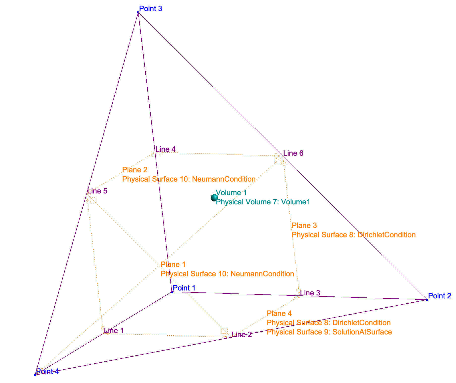
A general *.msh file contains much more information than we will discuss here. For more details, see the GMSH documentation. Here, we focus on the standard file obtained after generating (not so) simple geometries and meshes. We use the geometry shown in Figure 7 to illustrate the data arrangement in the mesh file and explain how to store the mesh information. The geometry is a tetrahedral domain with elements. During the *.msh storage, we chose the Save All options to store all the mesh information. For more detailed information, we refer the reader to duque2023integration and the official GMSH tutorial.
4.1 Physical Groups
During the geometry generation, it is possible to categorize the geometric entities used to construct by organizing them into physical groups. These groups allow us to associate the generated entities with specific material properties, boundary conditions, or other physical attributes important for simulation and post-processing. Figure 8 illustrates a typical example of this classification for the sample case. In the example considered, we observe that there are three 2D physical groups and only one 3D physical group.
$PhysicalNames
4
2 8 "DirichletCondition"
2 9 "SolutionAtSurface"
2 10 "NeumannCondition"
3 7 "Volume1"
$EndPhysicalNames
First, GMSH provides the number of Physical groups defined for a given geometry. Then it shows a list of the Physical groups, ordered by the dimension of the entities associated to the group and followed by both the numerical and string label. Naturally, it is also possible to set Physical group to zero- and one-dimensional entities, but this is not considered in our implementation.
4.2 Entities
This section list all geometric entities used to define the domain by using a boundary representation. Figure 9 illustrates the structure of this section for the sample case.
$Entities
4 6 4 1
1 0 0 0 0
2 1 0 0 0
3 0 1 0 0
4 0 0 1 0
1 0 0 0 0 0 1 0 2 1 -4
2 0 0 0 1 0 1 0 2 4 -2
3 0 0 0 1 0 0 0 2 2 -1
4 0 0 0 0 1 0 0 2 1 -3
5 0 0 0 0 1 1 0 2 3 -4
6 0 0 0 1 1 0 0 2 3 -2
1 0 0 0 1 1 1 1 10 3 5 2 -6
2 0 0 0 0 1 1 1 10 3 1 -5 -4
3 0 0 0 1 1 0 1 8 3 3 4 6
4 0 0 0 1 0 1 2 8 9 3 1 2 3
1 0 0 0 1 1 1 1 7 4 1 2 4 3
$EndEntities
The first row shows the number of entities for each dimension, starting from zero-dimensional to three-dimensional entities. The geometry consists of four points, six lines, four surfaces and one volume.
The entities are listed by dimension and their numerical label (first highlighted number on each row) as assigned during the geometry generation. In this example, the numerical indexing of the entities starts at one and is continuous, but this is not always the case. After the numerical label, it shows the minimum and maximum bounds for each coordinate.
The following highlighted numbers indicate the number of Physical Groups associated with an entity, followed by the numerical labels of the associated Physical Groups. In this example, all surfaces in the boundary and the volume have an associated Physical Group. Surfaces 1 and 2 are associated to NeumannCondition. Surface 3 and 4 are associated to DirichletCondition. Surface4 is also associated to SolutionAtSurface. Volume 1 is associated to Volume1.
The rest of the information in each row lists the entities of one dimension lower used to define the entity. The sign indicates whether the orientation of the embedded entity has been adjusted to match the orientation of the entity it is defining. If we refer back to Figure 7 and focus on Plane 2, we observe that this surface is constructed from three curves: Line 1, Line 4 and Line 5 (as can be seen in 3 1 -5 -4). Line 1 is an oriented segment from Point 1 to Point 4, Line 4 is oriented from Point 1 to Point 3 and Line 5 from Point 3 to Point 4 (see the respective rows). The orientation of the surface is defined following the direction of the first segment (in this case 1). The negative signs in the other lines are to match the orientation of Line 1 and achieve a coherent orientation in Surface 2. This definition for the orientation also applies for volumes using surfaces rather than curves.
4.3 Mesh
The mesh consists of nodes organized in elements (points, faces, edges and tetrahedra).
Nodes
The nodes within the mesh are given in Section Nodes. Figure 10 illustrates the structure of this section for the sample case.
$Nodes
15 7 1 7
0 1 0 1
1
0 0 0
0 2 0 1
2
1 0 0
0 3 0 1
3
0 1 0
0 4 0 1
4
0 0 1
1 1 0 0
1 2 0 1
5
0.5 0 0.5
1 3 0 0
1 4 0 0
1 5 0 1
6
0 0.5 0.5
1 6 0 1
7
0.5 0.5 0
2 1 0 0
2 2 0 0
2 3 0 0
2 4 0 0
3 1 0 0
$EndNodes
The first line details the number of entities that have stored data in this section, the total number of nodes in the mesh, and the minimum and maximum indices of those nodes. In this mesh, there are seven nodes, indexed from 1 to 7, organized into fifteen blocks. Each node uniquely appears within the interior of each entity. For each entity, there is a row that includes its dimension, numerical label, a parameter indicating whether the entity is parametric (which is always set to 0 for the cases of interest), and the number of associated nodes. Following this, the indices of all the nodes belonging to the entity are listed, one per row, along with their coordinates. For example, the nodes inside Line 5 are gathered in the block 1 5 0 1. This representation shows the entity dimensionality, its numerical label, and that it contains one node. The node is labeled with 6 and with coordinates .
In general, the indexing of the nodes is sparse. This can occur, for instance, when Save All is disabled, in which case nodes belonging to entities without an associated Physical Group are not stored, leading to missing nodes in the mesh file. To avoid this, we can enable Save All or add Physical Groups to all two- and three-dimensional entities. We redefine the indices so that the order is monotonic and there are no missing indices. The information of the coordinates of all nodes can then be stored in a matrix:
| (14) |
Elements
This section contains all the elements defined in the geometry and the nodes belonging to them. Figure 11 illustrates the structure of this section for the sample case.
$Elements
15 27 1 27
0 1 15 1
1 1
0 2 15 1
2 2
0 3 15 1
3 3
0 4 15 1
4 4
1 1 1 1
5 1 4
1 2 1 2
6 4 5
7 5 2
1 3 1 1
8 2 1
1 4 1 1
9 1 3
1 5 1 2
10 3 6
11 6 4
1 6 1 2
12 3 7
13 7 2
2 1 2 4
14 7 5 2
15 6 7 3
16 5 6 4
17 5 7 6
2 2 2 2
18 6 3 1
19 4 6 1
2 3 2 2
20 7 2 1
21 3 7 1
2 4 2 2
22 5 2 1
23 4 5 1
3 1 4 4
24 5 6 1 4
25 1 7 3 6
26 1 7 5 2
27 1 7 6 5
$EndElements
The first line specifies the number of element blocks (15), the total number of elements in the mesh (27), and the minimum (1) and maximum (27) indices of the elements in the mesh.
Each block represents an entity. It begins with a row that specifies the dimensions of the elements, the entity that contains these elements, the type of element, and the number of elements in the block.
We see four blocks containing elements of dimension 0 (with element type 15, according to GMSH). Each block contains a single element with indices 1 to 4, corresponding to nodes 1, 2, 3, and 4, respectively.
Following this are six consecutive blocks of dimension 1 (edges). These blocks contain 1, 2, 1, 1, 2, and 2 elements (with Element type 1), numbered from 5 to 13. Each block lists the nodes that define the edges. For example, the edges connect nodes 1 and 4, 4 and 5, 5 and 2, and so on.
Next, four blocks of dimension 2 (2D elements) are associated with the 2D entities with labels from 1 to 4. The first block contains four elements, while the remaining three contain two elements each. The elements are of type 2 (triangles), numbered from 14 to 23. The nodes defining each element are also provided. For instance, the first triangle is defined by nodes 7, 5, and 2, while the second is defined by nodes 6, 7, and 3.
Finally, a single block of dimension 3 is associated with the only three-dimensional entity, which contains four elements of type 4 (tetrahedra). The vertices defining these elements are also listed.
Triangular elements are oriented based on the orientation of the entities they belong to. To ensure that the elements are properly defined, the surfaces must be correctly oriented during the geometry generation. Our implementation assumes that this condition is met.
Even though the indexing of the elements can be sparse, we care about their order of appearance. We store the nodes belonging to each tetrahedral element in a matrix (for the case of tetrahedral elements):
| (15) |
such that for any given tetrahedron , the row contains the global indices of the nodes belonigng to the th tetrahedron.
Similarly, We can store the global indices for the triangles in the boundary in a matrix:
| (16) |
5 Finite Element Method
The Finite Element Method can be stated as follows
| (17) |
This discretizes the problem in the following sense: to solve (17), i.e., to find , we only need to determine the values of at the nodes outside the Dirichlet boundary. Thus, the number of unknowns is finite and is determined by requiring the solution to satisfy a test when multiplied by the elements of (a subspace of) , a finite-dimensional space. Indeed, let us define iD and inD to be the vectors containing the global indices of Dirichlet (where the exact solution is known) and non-Dirichlet (where it is not) nodes respectively. That is, iD and inD are a partition of the global indices,
and
Write as
The term is a discrete lifting of since for . Observe also that vanishes on . Therefore, with
FEM scheme becomes: (i) solve
| (18) |
and (ii) set next
The true unknowns are now
which determine and, by construction, the pointwise approximation of at the set of nodes of .
By linearity, we can restrict the test to the elements of any basis of , such as , resulting in the scheme
| (19) |
This means that the approximation of the solution via the Finite Element Method transforms the problem to the resolution of the linear system
| (20) |
where (see (17))
| (21) | ||||||
These terms are referred to as follows: in the first column, the stiffness matrix, the mass matrix, and the convection matrix. In the first term of the second column, the boundary mass matrix. The vectors in the second column are known as the load vector and the Robin vector, respectively.
6 Assembly
We next focus on the different vectors and matrices involved in the FEM, such as they are presented in (21), which can be computed.
6.1 Load vector. Why element-by-element implementation
Let us consider the load vector: for . Due to the linearity of the integral, we can decompose the integral over to the tetrahedra containing each node:
In other words, (cf. (15)), i.e., represents the local index of the node within the element .
The last integral can be computed or approximated by a quadrature rule. A possible implementation is given in Algorithm 1.
This approach requires two steps: first, searching for the elements to which node belongs, and then performing a loop to determine the local ordering of the node within . The first step is the most time-consuming, as it requires exploring all elements in the mesh for each node.
A more efficient method can be employed, assembling element by element. In essence, this approach can be understood as the result of interchanging the two loops in the initial version of the algorithm:
Line2 in Algorithm 2 serves as the foundation for the element-by-element computation by iterating through the rows of the element data ttrh. Line2 retrieves the global indices of the nodes associated with the th element. Due to the structure of the ttrh matrix, the second loop simplifies into a loop through its columns, allowing to obtain the global index simply as .
6.2 Robin vector
For the Robin vector we need to compute integrals
where is a triangle with vertices and edges () contained in the (Robin) boundary of the domain.
Clearly, unless for some . Then
| (22) | ||||
If ntrBR denotes the triangles on the Robin boundary, we have:
6.3 Mass matrices
Let us consider in this subsection the computation of the mass and Robin matrices
Any entry of the first matrix can be expressed as
| (23a) | |||
| where in the sum above | |||
| (23b) | |||
(Once again is the local index of the th global node in the element ). Similarly to the load and Robin vector, we identify in (23) three nested loops: the first two iterate over and , running on the nodes, and the third, the innermost one, is over , to locate the tetrahedron to which and belong. Using an element-by-element assembly, which effectively shifts the innermost loop to the outermost position, reorganizes these computations and simplifies the process, as demonstrated in the following algorithm
The Robin matrix can be handled in a very similar manner, reducing, after the change of variables, the assembly to compute the integrals element by element to
| (24) |
As a result, we obtain the following algorithm:
6.4 Stiffness Matrix
The assembly of the stiffness matrix is more involved as a consequence of combining the change of variable, which moves the computation to the reference element and the chain rule. Indeed, for a fixed and two nodes with indices , the stiffness matrix reduces to:
where
(That is, nodes and are the th and th in the local index of element ). The chain rule and the change of variables theorem yield then
Hence, denoting as usual the entries of the matrix function it holds
Therefore, the local stiffness matrix can be written in terms of nine local stiffness matrices
where
The assembly process is shown in Algorithm 6. The steps are now essentially the same. The only key difference is that more terms have to be computed for the assembly of the local matrix. The integrals are again computed using cubature rules.
6.5 Advection Matrix
Finally, we focus on the computation of
which is reduced, via the Change of Variables and the chain rule as:
where
The computation is then given:
Obviously, we are implicitly working with the local advection matrix that is written as
with
7 Key notes on FEM implementation in Matlab/Octave
This section deals with an implementation of the classical 3D -FEM algorithms with GMSH integration available in fem3d_gmsh . While a detailed discussion of the implementation is beyond the scope of this work, we refer the reader to duque2023integration for a more comprehensive explanation of the code.
7.1 Importing and preprocessing the mesh
We have implemented a function (importGMSH3D) to process a simple GMSH mesh exported in a *.msh file under the 4.1 version (as pointed out before, the latest version available at the time of this publication) in ASCII format. We also compute some other quantities that are used or can be used in the future for the FEM implementation. We will provide a brief commentary on these aspects.
Essential Boundary Conditions
Section 6 focuses on the computation of the matrices and vectors in (21) from where (5) can be easily constructed. Certainly, with
we obtain the system of equations:
C(inD, inD)u(inD) = d(inD) - C(inD, iD)u(iD),
where iD are the indices of Dirichlet nodes, for which the solution, i.e., , is known. We need to establish a structure to classify elements and nodes based on their boundary conditions. This classification is implemented as follows: a container structure is used, named, for instance, ComplementaryInformation, such that ComplementaryInformation("PhysicalName") retrieves a vector with the numerical labels of the entities belonging to the specified physical group.
The construction of this structure is straightforward. It involves storing the numerical and string labels of the Physical Groups mentioned in Section 4.1, looping through the entities (described in Section 4.2), and subsequently looping through the Physical Groups associated with each entity.
We then create the vector domain (resp. domBd) of size (resp. ), such that domain(m) (resp. domBd(m)) contains the numerical label of the entity to which the element belongs.
If we construct a Physical Group "Dirichlet" for the surface entities in , the triangular elements belonging to this boundary can be retrieved using
gammaD = ismember(domBd, ComplementaryInformation("Dirichlet"));
The indices of the Dirichlet nodes, iD, are obtained with
dirichletElements = trB(gammaD,:);
iD = unique(dirichletElements(:), :);
making the non-Dirichlet nodes available with
inD = setdiff(1:nNodes, iD);
Geometric mesh quantities
As detailed in the previous section, several (geometric) quantities of the mesh are used in the assembly of the different matrices and vectors (cf. (21)). We give a sketch of this procedure emphasizing the vectorized approach which gives rise to a free-loop fast code.
First the determinant of , i.e. the volume of the tetrahedra. This data is stored in a vector detBk so that . Matlab/Octave can compute all these quantities in a few lines by using the formula
as shown here: {programcode}Determinant in Matlab/Octave
v01 = coord(ttrh(:,2),:)-coord(ttrh(:,1),:);
v02 = coord(ttrh(:,3),:)-coord(ttrh(:,1),:);
v03 = coord(ttrh(:,4),:)-coord(ttrh(:,1),:);
detBk = dot(v01, cross(v02, v03, 2),2);
Let us briefly comment these lines. The matrix coord (see (14)) contains the coordinates of the all the nodes of the mesh, while ttrh(:,i+1) for returns the global indices of the vertices () as a column vector.
The first three lines compute matrices, where each row contains , , as described above. The functions dot and cross compute the dot and cross products of the row vectors of the matrices involved simultaneously, eliminating the need for explicit loops. Notice that the local indexing shown in Section 3.3 always makes the determinant positive.
A similar approach is followed for computing the non-normalized normal vectors to the triangles in the boundary and stores them in a matrix Bdnormal: {programcode}Normal vector to triangle in the boundary in Matlab/Octave
l1 = coord(trB(:,1),:) - coord(trB(:,2),:);
l2 = coord(trB(:,1),:) - coord(trB(:,3),:);
Bdnormal = cross(l1, l2, 2);
Precomputing these normal vectors rather than their modules allows us to extend the code to cases where the Robin/Neumann data is not the scalar field but a vector field such that (for example, scattering problems).
Faces and tetrahedra
Other geometric quantities, such as: (i) the faces (including inner faces) of the tetrahedra, (ii) the specific faces that form the tetrahedra, and (iii) the tetrahedra to which these faces belong, can be obtained by processing using commands like , , and . It is important to note that while this information is not utilized in our current implementation, it is necessary for calculating a posteriori FEM error estimates or for more advanced finite element methods, such as Discontinuous Galerkin schemes.
For illustrative purposes, the following code computes the faces (triangles) of the tetrahedra and store them in a matrix faces:
Computation of tetrahedron interfaces
indAux   = [2 3 4; 1 4 3; 1 2 4; 1 3 2];
faces  = [ttrh(:,indAux(1,:)); ...
          ttrh(:,indAux(2,:)); ...
          ttrh(:,indAux(3,:)); ...
          ttrh(:,indAux(4,:))];
facesAux = sort(faces(:,1:3),2);
[~,p1, p3]  = unique(facesAux,’rows’, ’first’);
faces     = faces(p1,:);
The variable indAux establishes an ordering for the vertices of all interfaces, ensuring that the normal vectors point outwards to the elements. We then define all faces in the mesh through their vertices. With this, it is just a matter of finding rows with a unique set of indices (up to permutation). We remove the permutation requirement by sorting out the index of the faces in a new variable facesAux. Finally, we find the first occurrence of all the interfaces to construct faces.
Next, the relation between tetrahedra and their faces and vice versa can be set with the following code:
Relationship between tetrahedrons and interfaces
ind = zeros(nTtrh,4); ind(:) = 1:numel(ttrh(:,1:4));
ttrh2faces  = p3(ind);
[~,p2]      = unique(facesAux,’rows’, ’last’);
p1  = mod(p1,nTtrh)    ; p1(p1==0) = nTtrh;
p2  = mod(p2,nTtrh)    ; p2(p2==0) = nTtrh;
faces2ttrh = [p1, p2];
ind = p1==p2;
faces2ttrh(ind,2) = nan;
We construct the matrix ttrh2faces and the matrix faces2ttrh. The former matrix contains, on each row, the indices of the four faces in faces belonging to a tetrahedron. The latter contains at each row the indices of the two tetrahedra (or one tetrahedron if the face lies in the boundary) in ttrh.
The variable ind enumerates the faces bounding every tetrahedron (ind(i,j) is the (i+j)-th row of facesAux, i.e., the j-th face belonging to the i-th tetrahedron). The index p3 defined in the previous computation contains the mapping of the indices of the unique faces in faces and all the faces. Hence we can construct ttrh2faces using p3(ind).
Notice that facesAux is a matrix. Each nTtrh block contains one of the faces of every tetrahedron in the mesh. With mod, we restore the index of the tetrahedron associated with that face (except for the special case of the last tetrahedron, which we readjust to nTtrh). The pair of tetrahedra containing each face are the indices of the first and last appearance of a face in facesAux. To make boundary faces easily accessible and avoid redundant information, we set the second value to nan by looking for the cases where the tetrahedron indices repeat in a row. We store this information in faces2ttrh.
7.2 Vector and matrix assembly
Let us consider the assembly of the load vector. To achieve this, we apply a quadrature formula using appropriate weights and nodes , provided in barycentric coordinates within the reference element , such that
(Notice that, for the sake of convenience, we have written in terms of barycentric coordinates instead of Cartesian variables, as they were originally introduced.) The computation of these terms in Matlab can be implemented as follows:
Quadrature formula approach for computing load vector
Nr = zeros(dofK, nQ);
for i = 1:dofK
    Nr(i,:) = Nj3D{i}(nodesQuad(1,:),nodesQuad(2,:),...
                            nodesQuad(3,:),nodesQuad(4,:));
end
px = coord(:,1); py = coord(:,2); pz = coord(:,3);
nodesX = px(ttrh(:,1:4))*nodesQuad;
nodesY = py(ttrh(:,1:4))*nodesQuad;
nodesZ = pz(ttrh(:,1:4))*nodesQuad;

val = f(nodesX, nodesY, nodesZ).*detBk;
Nr = repmat(Nr,nTtrh,1);
val = repelem(val,dofK,1);
val = val.*Nr;
val = val*weights(:)/6;
Let us describe the code briefly since it illustrates the techniques we use to assemble the right-hand-side vector.
To compute the integral, we need to evaluate both the shape functions and the source term at the quadrature nodes, which are specified in barycentric coordinates in the matrix nodesQuad. The shape functions have been previously stored in the cell structure Nj3D as four-variable functions of the barycentric coordinates. This evaluation is performed in the first four lines of the previous code.
To evaluate , we first compute the quadrature nodes for all elements of the mesh, i.e., the action of the affine mapping on the quadrature nodes in the reference element via (11) in Lines 6-9. The expression px(ttrh(:,1:4)) produces a matrix where each row contains the -coordinate of the vertices of all tetrahedra. As a result, nodesX is an matrix that stores, row by row, the -coordinate of the quadrature nodes within all elements. A similar structure applies to nodesY and nodesZ for the y- and z-coordinates, respectively.
Lines 11–14 evaluate at the quadrature nodes for each element . Note that a column-wise matrix-vector operation (".*") is applied twice: first, to incorporate into the values of , and second, to multiply these values by the values of all shape functions at the quadrature nodes.
The final line computes the action of the quadrature rule and stores the results in blocks, each of size . These blocks are then concatenated into a vector of length .
Let us emphasize that this code can be easily modified to handle functions with an extra (fourth) variable to indicate the physical group to which each element belongs. This facilitates the straightforward definition of piecewise-defined functions for the load vector.
The assembly of the load vector can be implemented in a vectorised way in just three lines: {programcode}Assembly of load vector
indi = T.ttrh’;
indi = indi(:);
b =  accumarray(indi, val, [nNodes, 1]);
The validity of these lines is far from trivial. The construction of indi is somewhat delicate, requiring careful attention to order the data stored in val. The function accumarray facilitates the construction of vectors by inserting val(i) (recall Matlab uses column-major order) at the position indi(i), adding up values in cases of repeating indices. These lines complete the computation of the inner loop in Algorithm 2 in a vectorized manner.
This process is extended to compute the matrices in the system of equations, following similar steps. For instance, for the mass matrix, we proceed as follows: (a) compute at the quadrature nodes and store the results in a matrix; (b) evaluate the function at the quadrature nodes for all tetrahedra and store the result in a vector precisely in the same manner as was evaluated in the previous code; (c) use repmat and repelem, column-wise product “” to construct a matrix, which is then multiplied by and to compute the action of the quadrature rule (this matrix contains the required quantities conveniently stored); (d) assemble the matrix using sparse (in place of accumarray) with suitable indices vector indi,indj.
We also need to compute for the stiffness and advection matrices. We can exploit vectorization using the following representation of the inverse matrix:
which results in {programcode}Computation of coefficients of inverse matrices
v01 = coord(ttrh(:,2),:)-coord(ttrh(:,1),:);
v02 = coord(ttrh(:,3),:)-coord(ttrh(:,1),:);
v03 = coord(ttrh(:,4),:)-coord(ttrh(:,1),:);
b1 = cross(v02,v03,2)./detBk;
b2 = cross(v03,v01,2)./detBk;
b3 = cross(v01,v02,2)./detBk;
Matrices b1, b2 and b3 contain, row-wise, the first, second, and third column of for all elements ,
7.3 Postprocessing of the FEM solution
After solving the linear system, we may want to evaluate the solution at arbitrary points. This requires, for each , identifying first the element containing and evaluating next the polynomial . The implementation follows these steps:
-
1.
Compute the barycentric coordinates for all elements (or a subset of them where is known to be).
-
2.
Find the element of nodes for which all barycentric coordinates are non-negative.
-
3.
Compute
Step three can be implemented as a dot-product as follows: Set the vector with
Then
For multiple points, such an evaluation can be performed by stacking these vectors into an matrix, . Note that is sparse. Once constructed, it can be reused to evaluate multiple solutions at the same points by simply performing the matrix-vector multiplication .
This approach can be implemented with manageable resource requirements for a modest number of points. However, if the solution needs to be evaluated at a large number of points, the memory requirements for performing this computation in a vectorized manner increase significantly. This challenge can be addressed if some a priori knowledge about the locations of the points is available.
8 Numerical examples
We present numerical examples across a range of different phenomena to demonstrate the implementation of our software fem3d_gmsh . The first two numerical simulations were performed on a MacBook Pro equipped with an Apple M3 chip, 16 GB of RAM, and running macOS Sonoma 14.5. The third experiment, however, was conducted on a Linux machine running CentOS Linux release 7.3.1611 with processors Intel(R) Xeon(R) CPU E5-2620 v4 @ 2.10GHz and 128 GB of RAM. All linear systems were solved using direct methods: either with the “\” command (mldivide), or, in the third experiment, through an factorization of the matrix (combined with suitable sorting algorithm to minimize the fill-in effect in the sparse matrix).
8.1 Heat equation
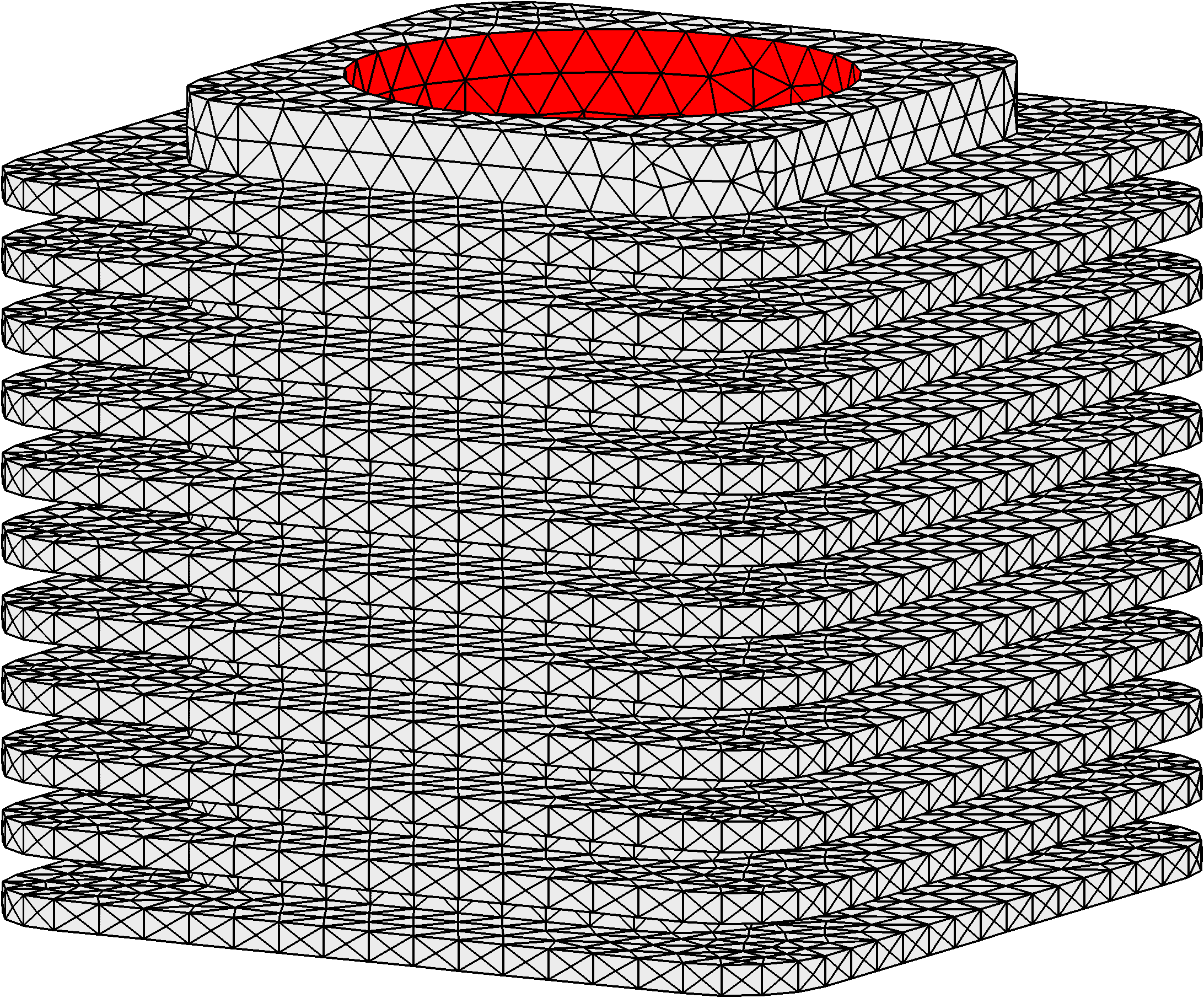
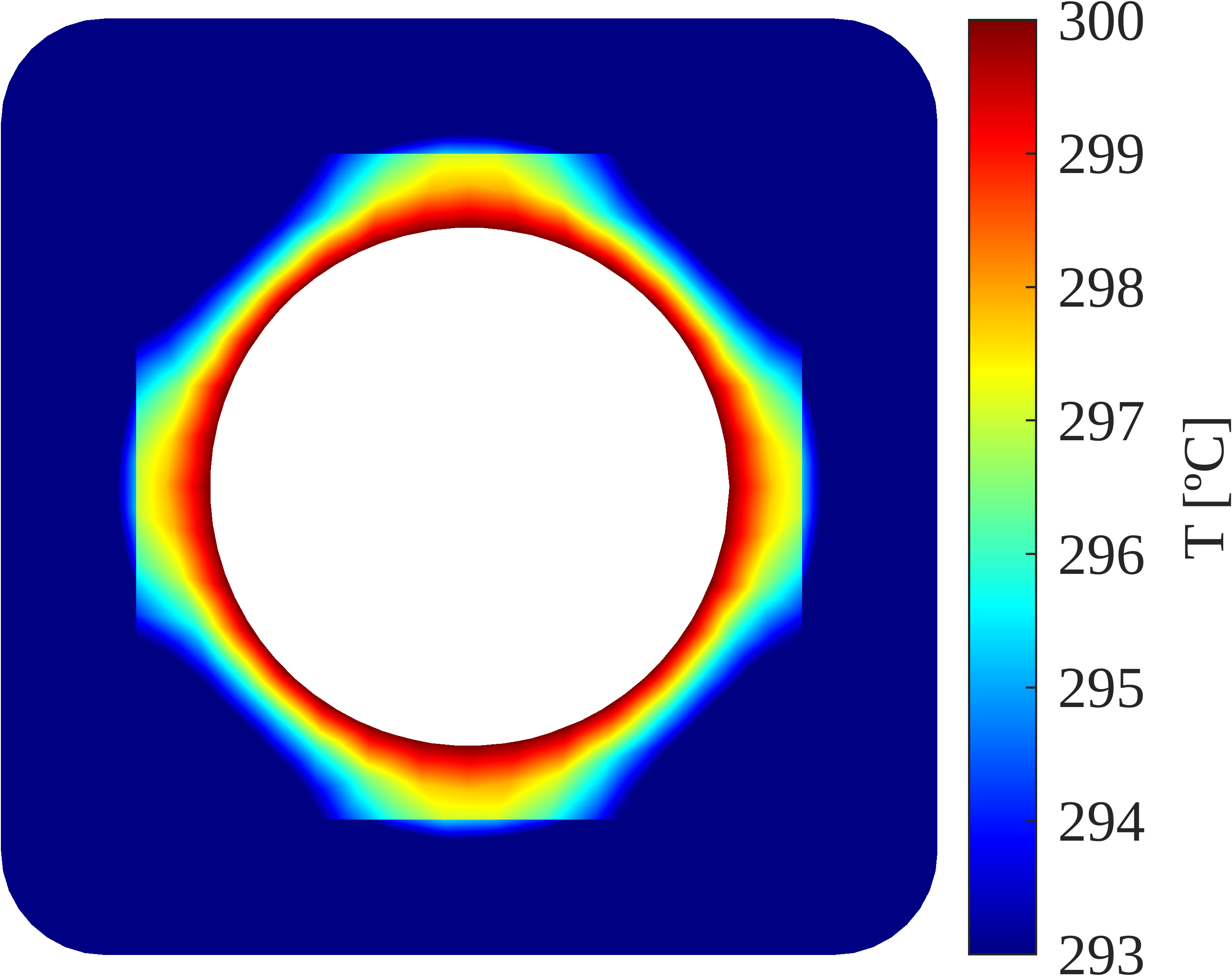
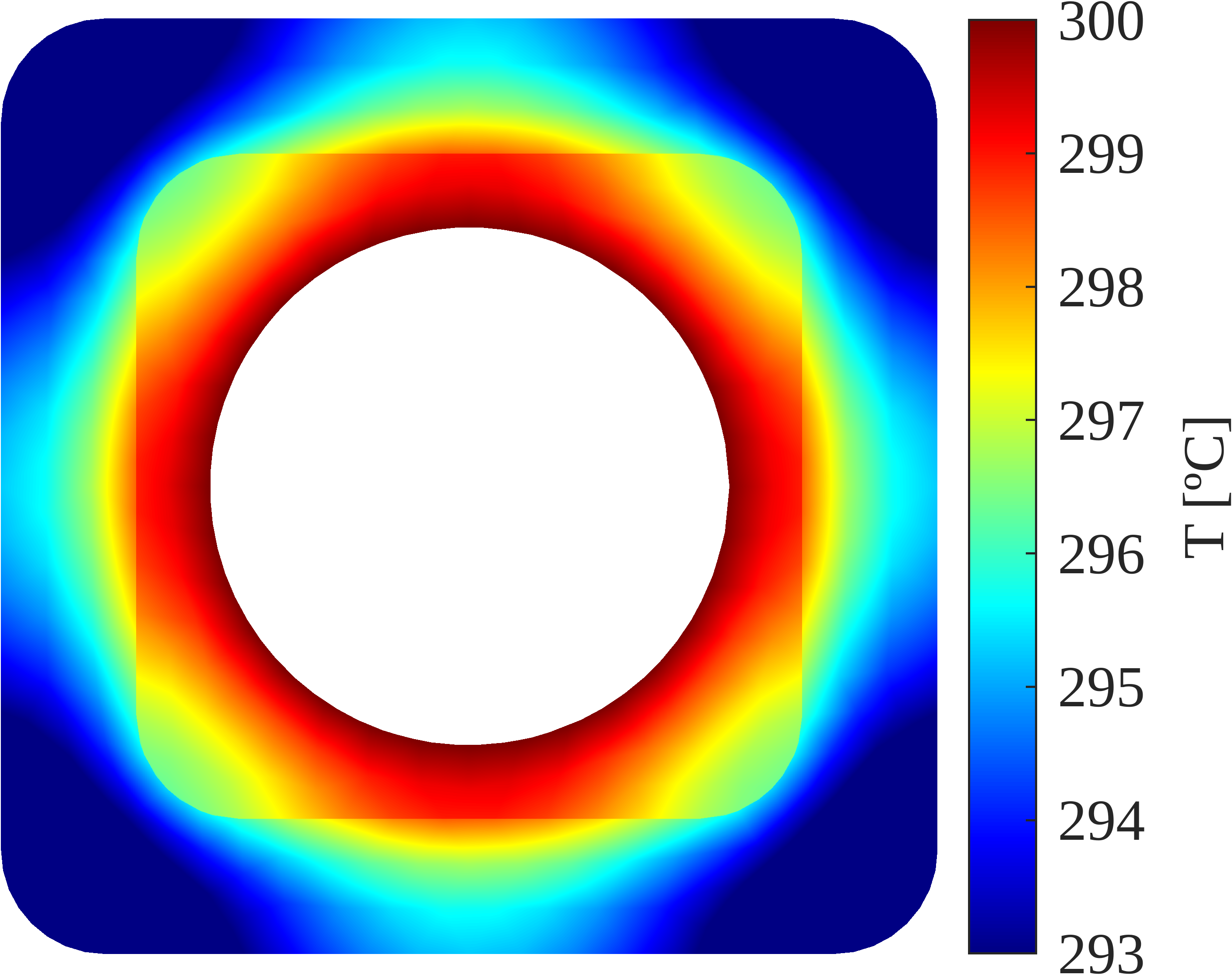
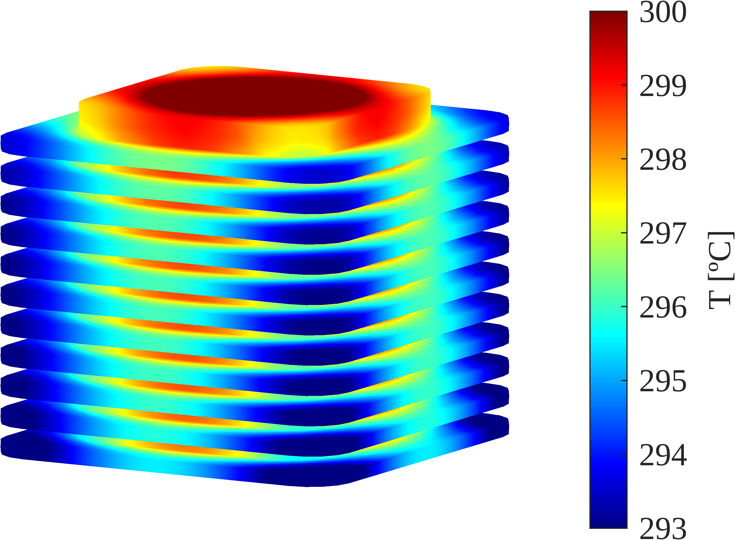
We first solve the heat equation
over an aluminum-finned engine cylinder (see Figure 12(a)). The properties of this material are: a density , heat capacity , and thermal conductivity .
Such a complex model has been constructed using free CAD software, FreeCAD freecad , exported in STL format, and processed in GMSH.
We use elements for this simulation. Constructing the entire data structure takes 0.82 seconds. The mesh comprises 28,979 tetrahedral elements, 17,322 triangular elements on the boundary, and 9,229 nodes. Given the entity-based structure of the *.msh file and the nature of the pre-processing computations, the cost of this function primarily depends on the number of elements. It is, therefore, remarkable how efficient vectorized code is in Matlab.
We consider an initial temperature over the whole body of C except for the Dirichlet condition (in red) with a constant temperature C. For the rest of the surfaces, we consider that there is dissipation due to convection:
where C is the temperature of the surrounding air and C is the convection coefficient. This is implemented as a Robin condition by equalizing this term with the heat flux at the Robin boundary.
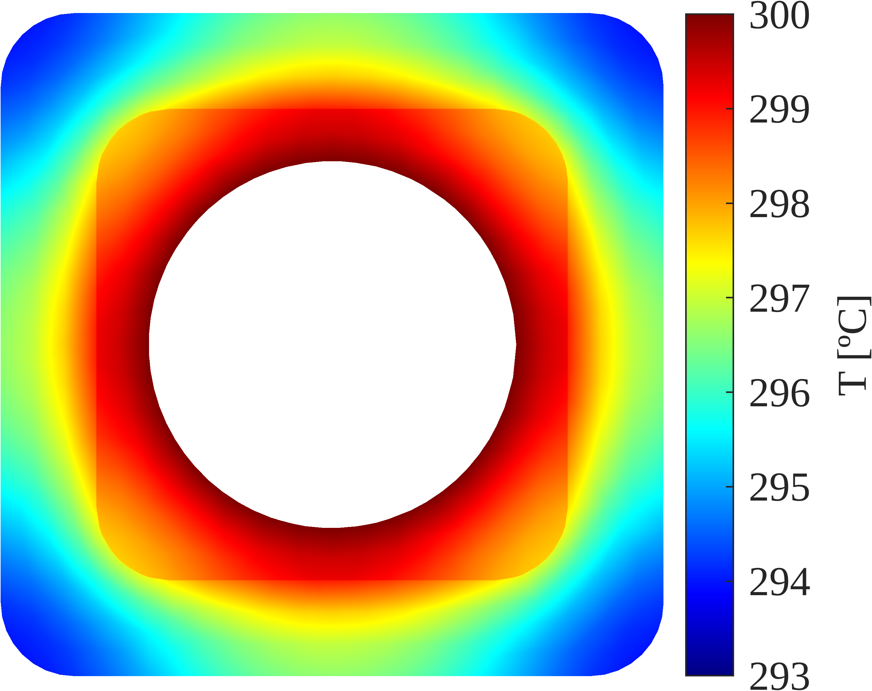
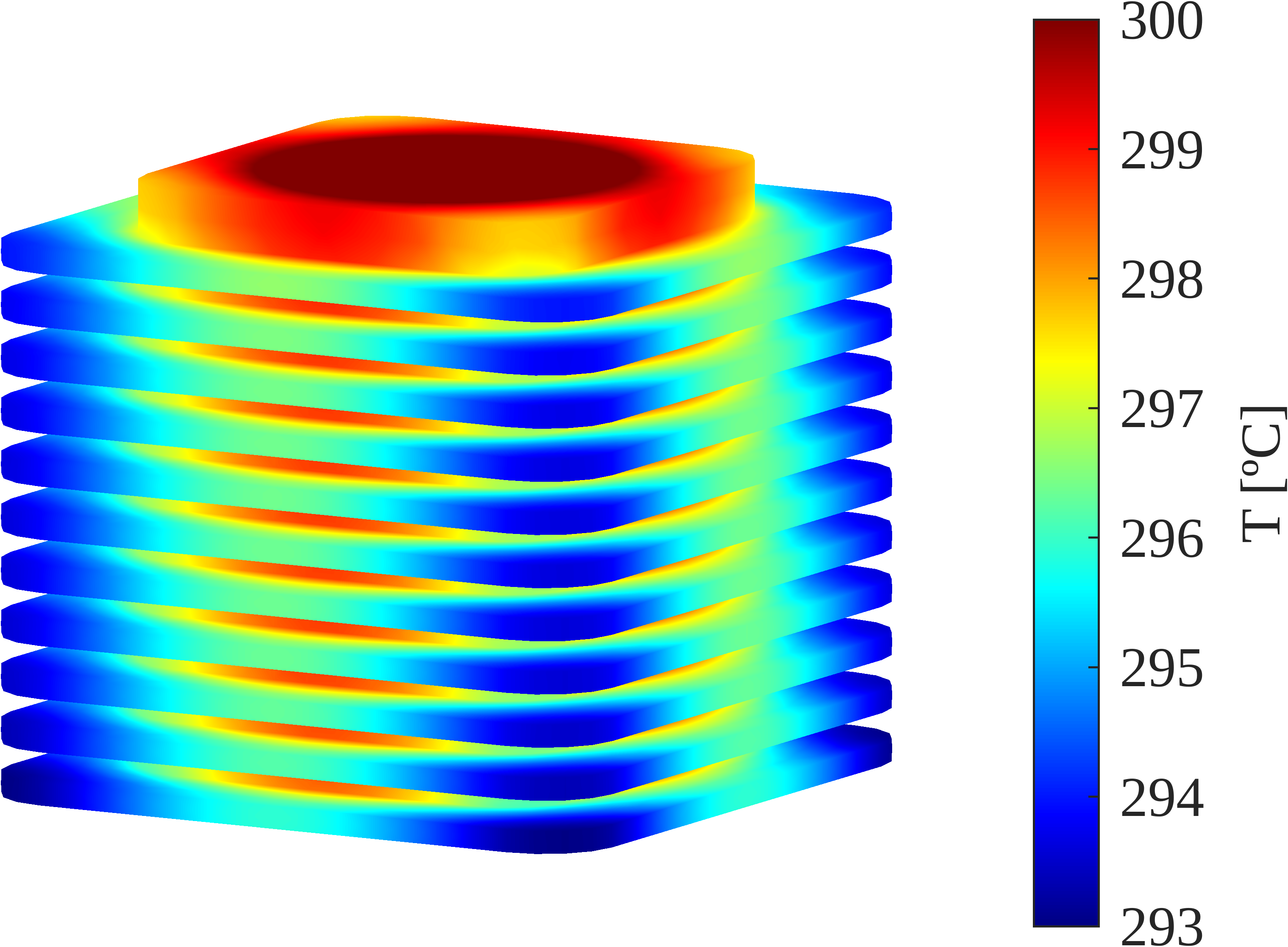
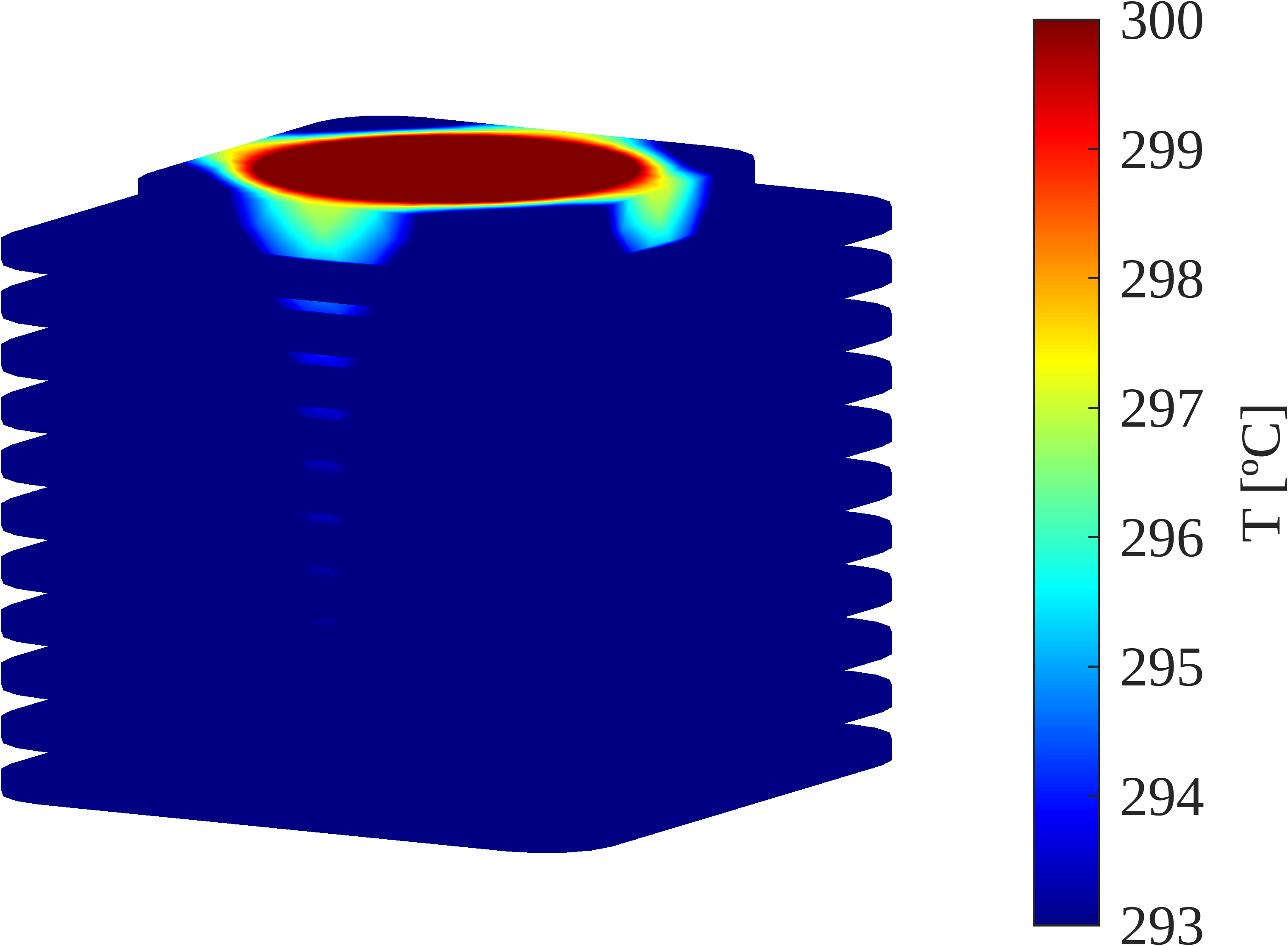
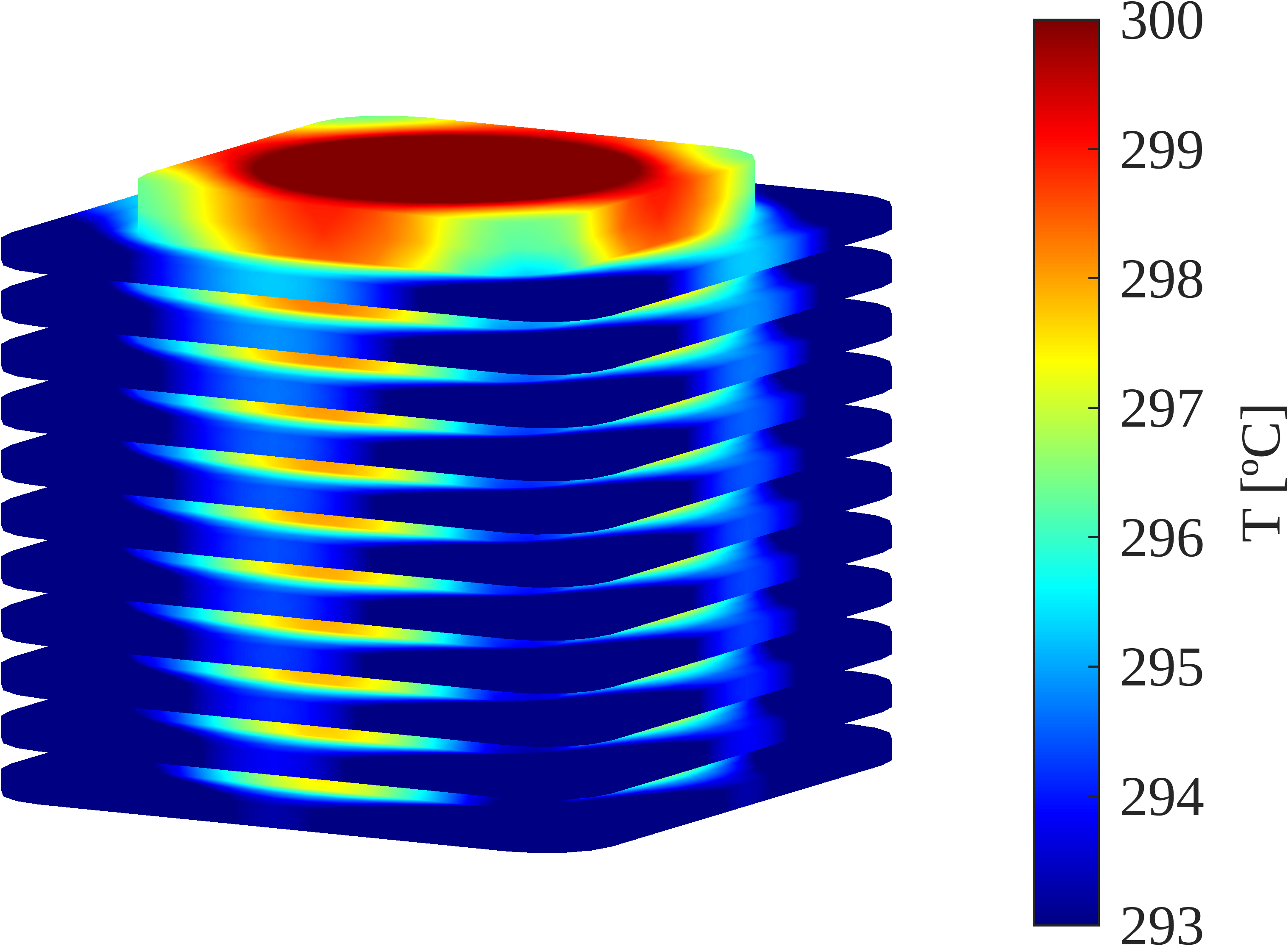
The stiffness matrix is computed exactly since is constant. The computation of the stiffness matrix and the Robin mass matrix and the Robin vector takes 0.03 s for their assembly. Figure 12b-c the solution to the steady state. In this case, we notice that neither and play a role in heat diffusion. All boils down to a balance of the diffusion term with the convection term at the boundary. With this solution, we see the importance of fins in bodies. They allow extending the heat flow region, hence reducing the overall maximum temperature by increasing the surface of contact with the surrounding air.
We also perform a transient simulation to see the evolution of the heat flow through the cylinder. The assembly of the mass matrix takes around 0.026 s. We integrate from to s. We use a Crank-Nicolson scheme to obtain the same second-order spatial and temporal discretization convergence. We choose a time step s. In total, it takes 4 minutes and 50 seconds to solve around 2400 time steps. The results of the numerical simulations are given in Figure 13.
s
s

s
s
s
s
The temperatures shown in the plots are bounded by the extreme values in the steady state to represent how each point in the cylinder reaches its steady state temperature.
8.2 Eigenvalue problem in elasticity
To demonstrate the capabilities and flexibility of this package, we also illustrate how it can be extended to other problems, such as the linear elasticity problem. This problem consist in finding the deformation field satisfying
where
is the stress tensor. Here, is the identity matrix, and are the Lamé constants and
is the linearised deformation tensor.
The basis used to describe the finite element space is given by , where , with the unit vector in the th direction. Ignoring the Dirichlet condition, and integrating by parts, the weak formulation can be written as
where denotes the usual Frobenius product. The solution is approximated as
We can easily show that for :
The discretized system of equations become
where is the stiffness matrix with diffusion matrix .
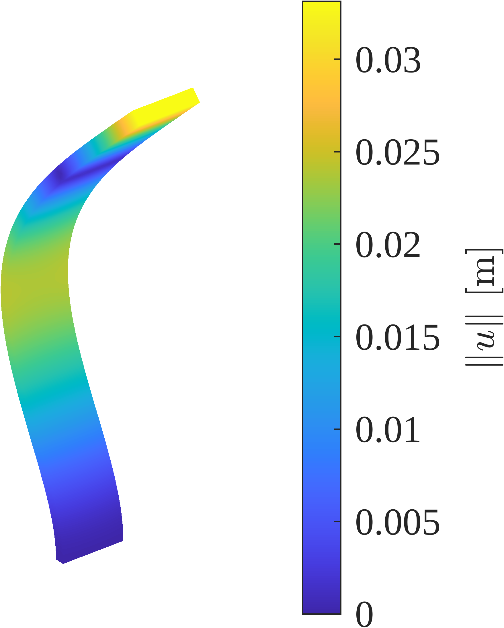
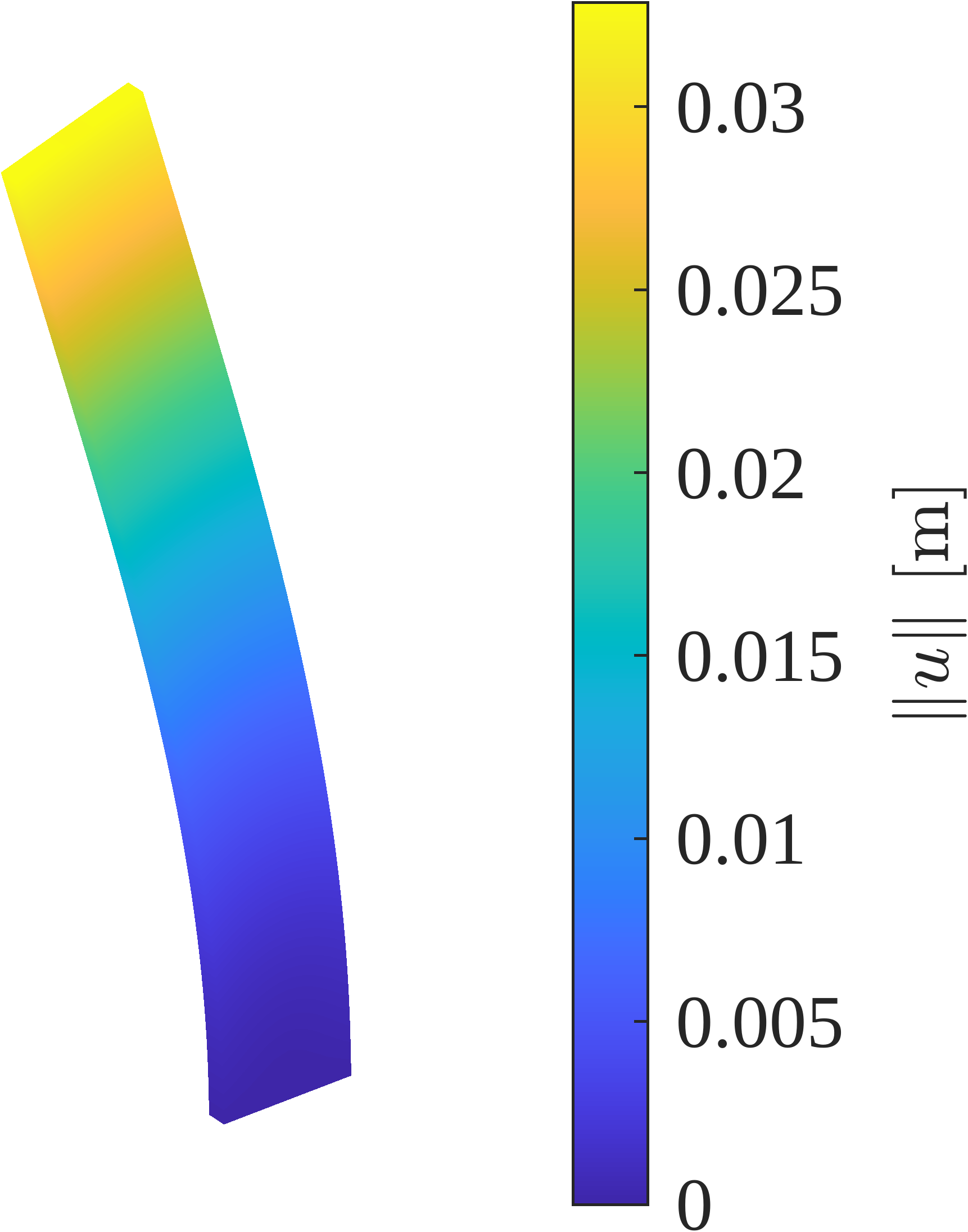
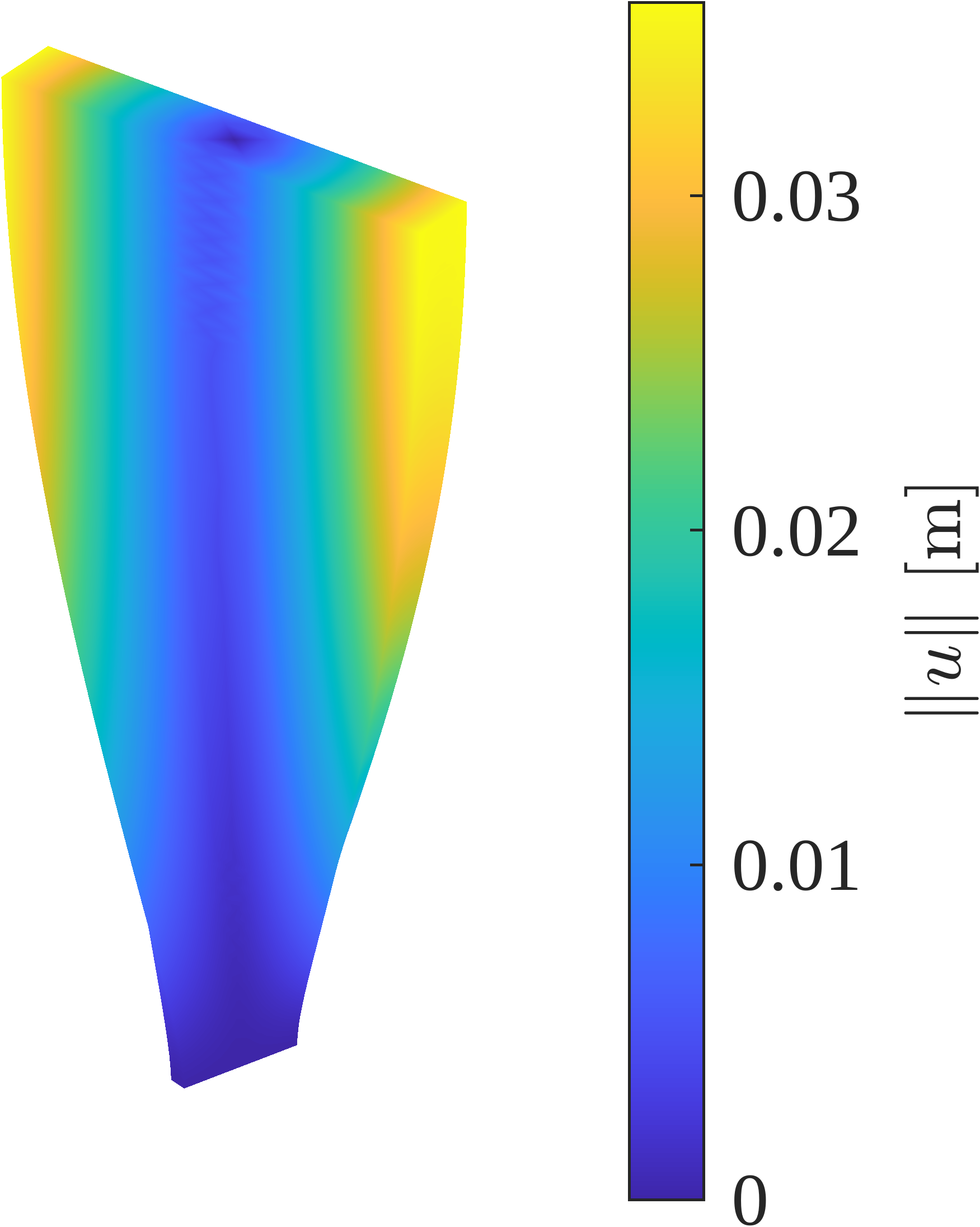
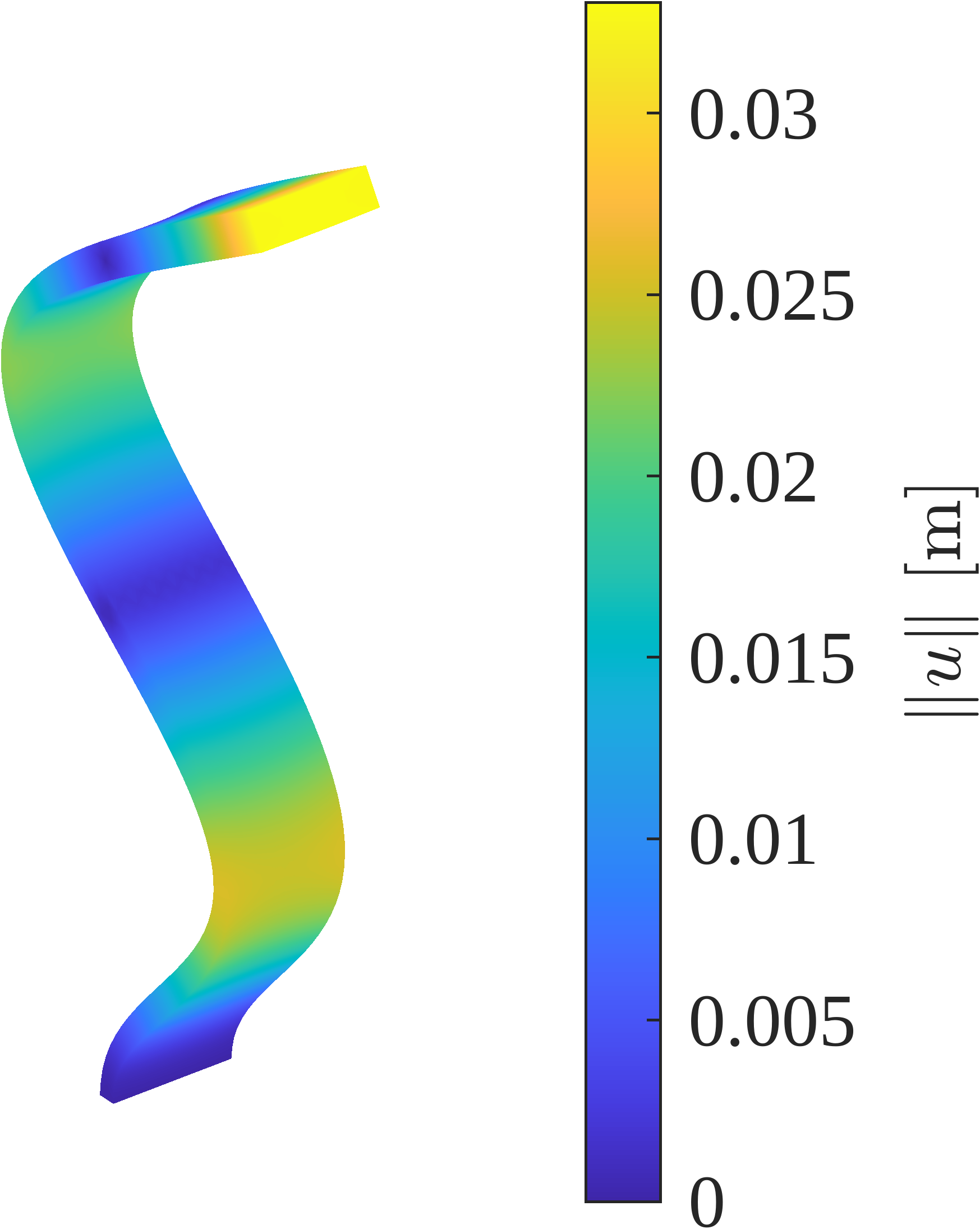
We solve the eigenvalue problem in elasticity. This corresponds to finding the natural frequencies of the geometry. We use -elements since FEM requires a large number of elements to see convergence.
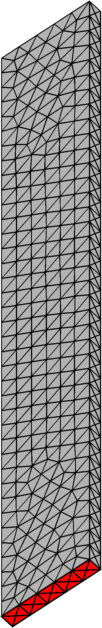
We consider a rectangular beam (see Figure 14(a)) with a length m, a width m, and thickness m. We fix one of the ends of the beam (highlighted in red). For material properties, we consider steel with density , Young modulus GPa, and poisson ratio . The Lamé parameters are determined from the relations
Therefore, GPa, which is not a very large value, makes using more sophisticated elements to address the locking phenomenon unnecessary.
The eigenvalue problem becomes finding such that
The right-hand side term adds a block-diagonal matrix with three mass matrices on each non-zero block term on the discretized problem. As usual in engineering applications, we compute the natural frequencies as
The mesh consists of 1,656 tetrahedra and 3,557 nodes. The computation of the stiffness matrix is more complex, as it now requires nine calls to the function that assembles the stiffness matrix in the scalar case. The assembly of the enlarged stiffness matrix takes 0.257 seconds, while the assembly of the enlarged mass matrix takes 0.012 seconds.
We compute the five lowest natural frequencies using the Matlab function eigs. The solutions are shown in Figures 14b-f. We see two bending modes parallel to the axis with the minimum moment of inertia (i.e., the width of the beam). In the third mode, a bending mode occurs along the perpendicular axis to the previous one (parallel to the thickness of the beam). A torsional mode is observed for the fourth mode. The increase in beam size arises from the inherent limitation of linear elasticity, which assumes small deformations and does not accurately model large rotations. Finally, the fifth mode represents another bending mode parallel to the width of the beam.
geometry

Hz
Hz
Hz
Hz
Hz
8.3 3D harmonic acoustic scattering
Let us consider the following acoustic scattering problem by a bounded domain in harmonic regimen:
| (25) |
Here is the wave-number, and is the so-called function of refractive index, with in the exterior . On the other hand, is a plane incident wave, a solution of the Helmholtz equation (with in the full space ). Therefore, is a unit vector indicating the direction of propagation of the incident wave, and is the so-called scattered wave.
This problem is naturally posed in the full domain, which makes the imposition of the boundary condition at infinity—that is, the radiation condition—challenging. Among several options, a very attractive choice is to combine the Finite Element Method (FEM) with Boundary Element Methods (BEMs). In BEM, the solution in the exterior of a bounded domain is expressed via an integral formula involving new unknowns defined only on the boundary. The radiation condition is then satisfied naturally. This BEM-FEM combination leverages the strengths of both methods: the flexibility of FEM for handling inhomogeneities and the capability of BEM for computing the solution sufficiently far away from the object , as well as for determining quantities of interest such as the far field, the asymptotic behavior of the scattered wave at infinity.
We do not intend to provide even a brief introduction to BEM-FEM coupling here. Instead, our goal is to illustrate how GMSH can handle complex domains, demonstrate the flexibility of our code in processing the returned meshes and show how our FEM solver can be integrated with available BEM codes. For details on the BEM solver used in this experiment, definition, implementation and convergence properties (which, under ideal conditions like those presented here, are superalgebraic) we refer to GaGr:2004 . The BEM-FEM coupling strategy followed in this experiment is detailed in DoGaSa:2020 .
Hence, consider the index refractive function given by
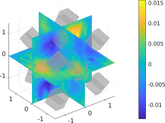
Here and are two halves (blue and red) of each of eleven cubes (so ) of edge 0.3. This configuration represents a simple model of what is known in the literature as a Janus particle: particles formed by two substances of the same shape glued together. The choice of these parameters is not accidental: 1.333 and 1.496 are, respectively, the refractive indices of water and toluene at 20∘C, which are commonly used in such particles. A schematic of the domains as well as an initial mesh (only on the boundary of the FEM domain) is sketched in Figure 15. For the incident wave we took and .
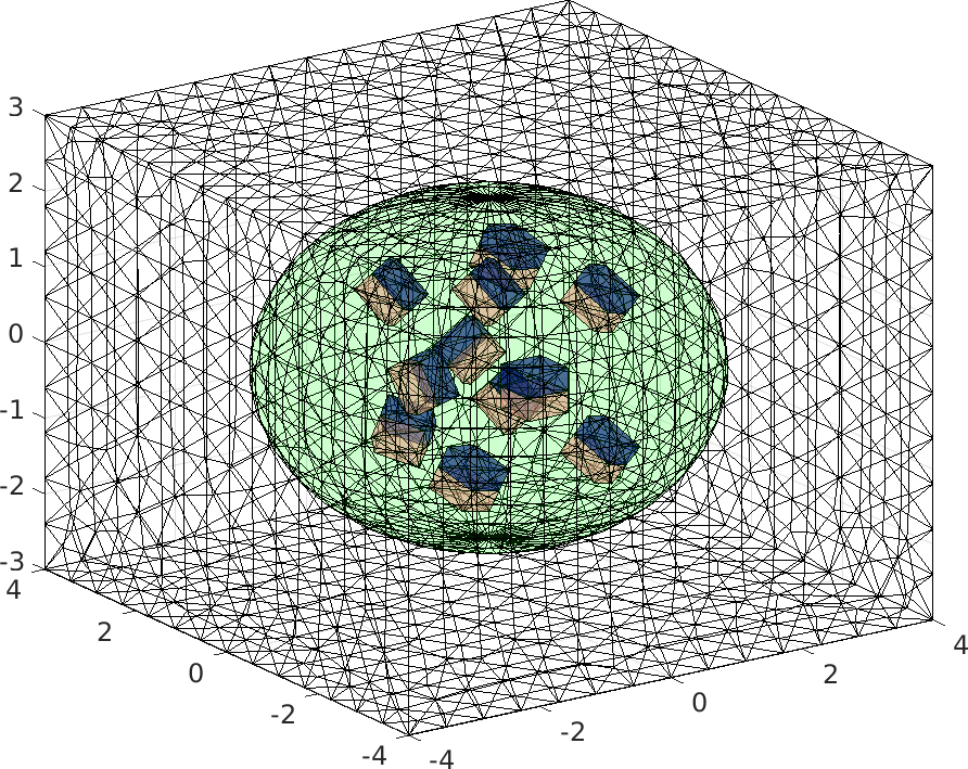 |
We used quartic elements (denoted as in our notation) for the FEM part and compared the solutions obtained at two consecutive levels of refinement to assess the quality of our numerical solution. To clarify, by ”consecutive refined meshes,” we mean the following:
In 3D, unlike in 2D, it is impossible to split a tetrahedron into eight or any arbitrary number of similar elements. Instead, in Gmsh, 3D mesh generators first create a mesh for the (2D) boundaries, which serves as the foundation for generating the corresponding 3D mesh. The process starts with the previous boundary (triangular) mesh for a refined mesh, refines it uniformly (using RGB refinement), and then constructs the next-level 3D mesh based on this refined boundary.
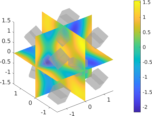
The number of elements is approximately 10,700 and 76,000 for the coarse and fine meshes, respectively, corresponding to around 124,000 and 845,000 nodes. The problem is large enough to require a machine with substantial memory capacity since the linear system in the FEM part is solved using a direct method, specifically factorization. The effect of the BEM scheme on convergence is negligible for two reasons: the fast convergence of the BEM scheme itself and the sufficiently large number of degrees of freedom.
The (real part of the) solution on the coarse mesh and the discrepancy between the FE solutions on the coarse and fine meshes is plotted on three conveniently chosen perpendicular planes, as shown in Figure 16. This visualization also demonstrates the evaluation and postprocessing of the solution, as discussed in subsection 7.3.
Acknowledgments
The first author thanks the support of projects “Adquisición de conocimiento y minería de datos, funciones especiales y métodos numéricos avanzados” from Universidad Pública de Navarra, Spain and “Técnicas innovadoras para la resolución de problemas evolutivos”, ref. PID2022-136441NB-I00 from Ministerio de Ciencia e Innovación, Gobierno de España, Spain. The second author thanks the support of the Basque Center of Applied Mathematics (BCAM) and the support of the project “Proyecto I+D+i 2019: Inversión de datos en tiempo real usando métodos de aprendizaje profundo (DEEPINVERSE)”, ref. PID2019-108111RB-I00 from Ministerio de Ciencia e Innovación, Gobierno de España, Spain.
References
- [1] J. Alberty, C. Carstensen, and S.A. Funken. Remarks around 50 lines of Matlab: short finite element implementation. Numer. Algorithms, 20(2-3):117–137, 1999.
- [2] M.S. Alnaes, J. Blechta, J. Hake, A. Johansson, B. Kehlet, A. Logg, C.N. Richardson, J. Ring, M.E. Rognes, and G.N. Wells. The FEniCS project version 1.5. Archive of Numerical Software, 3, 2015.
- [3] C. Bahriawati and C. Carstensen. Three MATLAB implementations of the lowest-order Raviart-Thomas MFEM with a posteriori error control. Comput. Methods Appl. Math., 5(4):333–361, 2005.
- [4] S.C. Brenner and L.R. Scott. The Mathematical Theory of Finite Element Methods, volume 15 of Texts in Applied Mathematics. Springer, 3rd edition, 2008. A comprehensive guide on the mathematical foundations of the finite element method.
- [5] C. Carstensen and R. Klose. Elastoviscoplastic finite element analysis in 100 lines of Matlab. J. Numer. Math., 10(3):157–192, 2002.
- [6] P.G. Ciarlet. The Finite Element Method for Elliptic Problems, volume 4 of Studies in Mathematics and its Applications. North-Holland, Amsterdam, 1978. A classic foundational text in finite element theory.
- [7] FreeCAD Community. FreeCAD: an open-source parametric 3d cad modeler, 2025.
- [8] V. Domínguez, M. Ganesh, and F. J. Sayas. An overlapping decomposition framework for wave propagation in heterogeneous and unbounded media: formulation, analysis, algorithm, and simulation. J. Comput. Phys., 403:109052, 20, 2020.
- [9] A. Duque-Salazar. FEM3D_GMSH: Finite Element Method with 3D meshes generated by GMSH. https://github.com/aleduques/FEM3D\_GMSH, 2023.
- [10] A. Duque-Salazar. Integration of the meshing tool gmsh with matlab/octave for the resolution of 3d boundary value problems with simplicial finite elements, 2023.
- [11] A. Ern and J.-L. Guermond. Theory and practice of finite elements, volume 159 of Applied Mathematical Sciences. Springer-Verlag, New York, 2004.
- [12] A. Ern and J.-L. Guermond. Finite elements I—Approximation and interpolation, volume 72 of Texts in Applied Mathematics. Springer, Cham, [2021] ©2021.
- [13] A. Ern and J.-L. Guermond. Finite elements II—Galerkin approximation, elliptic and mixed PDEs, volume 73 of Texts in Applied Mathematics. Springer, Cham, [2021] ©2021.
- [14] F.-J. Sayas et collaborators. Team pancho website, 2025. Accessed: 2025-01-17.
- [15] S.A. Funken, D. Praetorius, and L.K. Rüde. Efficient implementation of adaptive P1-FEM in Matlab. Comput. Methods Appl. Math., 11(4):460–490, 2011.
- [16] M. Ganesh and I. G. Graham. A high-order algorithm for obstacle scattering in three dimensions. J. Comput. Phys., 198(1):211–242, 2004.
- [17] C. Geuzaine and J.-F. Remacle. Gmsh: A 3-d finite element mesh generator with built-in pre- and post-processing facilities. International Journal for Numerical Methods in Engineering, 79(11):1309–1331, 2009. An open-source tool for finite element mesh generation and post-processing.
- [18] F. Hecht. New development in FreeFem++. J. Numer. Math., 20(3-4):251–265, 2012.
- [19] F.-J. Sayas. An introduction to the finite element method, 2015. Accessed: 2024-11-28.
- [20] F.-J. Sayas and collaborators. FEM tools in three dimensions. Unpublished document, personal communication, n.d.
- [21] E.P. Stephan. Coupling of Boundary Element Methods and Finite Element Methods, pages 1–40. John Wiley & Sons, Ltd, 2017.
- [22] O.J. Sutton. The virtual element method in 50 lines of MATLAB. Numer. Algorithms, 75(4):1141–1159, 2017.
- [23] O.C. Zienkiewicz and R.L. Taylor. The Finite Element Method: Its Basis and Fundamentals. Elsevier, 7th edition, 2013. A comprehensive introduction to FEM with a focus on fundamentals and applications.