On grid homology for diagonal knots

Abstract.

We partially determine grid homology for diagonal knots, a class of knots including Lorenz knots that can be represented by a good grid diagram in some sense. We compare diagonal knots to some class of knots such as positive braids, fibered positive knots, and $L$-space knots.

1. Introduction

Grid homology is a combinatorial invariant of knots in $S^{3}$ and is isomorphic to knot Floer homology [12]. Sarkar [21] gave a combinatorial proof of the Milnor conjecture [13] using grid homology. Sarkar observed that for torus knots, the tau invariant, a concordance invariant in knot Floer homology, can be easily calculated using grid diagrams as in Figure 1. Arndt-Jansen-McBurney-Vance [1] defined a diagonal knot as a knot represented by such a grid diagram.

Definition 1.1.

A grid diagram is diagonal if its $O$-markings are on the diagonal from top left to bottom right.

Definition 1.2 ([1, Definition 2.2]).

A knot is called diagonal if it is represented by a diagonal grid diagram.

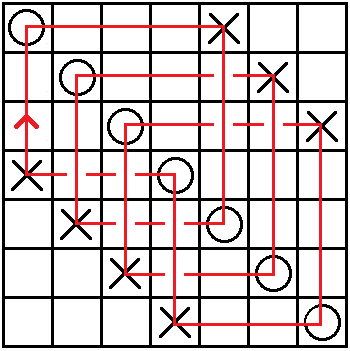
Figure 1. A torus knot $T(4,3)$ and a diagonal grid diagram representing it.

A knot is called positive if it admits a diagram consisting only of positive crossings. Arndt-Jansen-McBurney-Vance studied diagonal knots to prove the following.

Theorem 1.3 ([1, Theorem 3.3]).

Diagonal knots are positive.

It is easy to see that torus knots and connected sums of diagonal knots are diagonal. On the other hand, the following holds.

Theorem 1.4 ([1, Theorem 3.5]).

There is a diagonal knot which is neither a torus knot nor a connected sum of torus knots.

Arndt-Jansen-McBurney-Vance found such a knot represented by a diagonal grid diagram of size $11\times 11$. According to them, SnapPy says it is SnapPy census knot $m211$.

Razumovskiĭ [20, 19] also studied links represented by a diagonal grid diagram. Lorenz links are periodic orbits in the flow in $\mathbb{R}^{3}$ determined by the Lorenz differential equations, well-known differential equations as a chaotic dynamical system [4]. It is known that a Lorenz link has a braid representation as

$$(\sigma_{1}\cdots\sigma_{p_{1}-1})^{q_{1}}(\sigma_{1}\cdots\sigma_{p_{2}-1})^{q_{2}}\cdots(\sigma_{1}\cdots\sigma_{p_{k}-1})^{q_{k}},$$

for some $2\leq p_{1}<\dots<p_{k}$ and $q_{i}>0$ $(i=1,\dots,k)$ [3].

Theorem 1.5 ([20]).

Every Lorenz link is represented by a diagonal grid diagram.

Theorem 1.6 ([19]).

Diagonal knots are fibered.

Remark 1.7.

• Razumovskiĭ defined a diagonal link as a link represented by a diagonal grid diagram satisfying a certain condition and proved that diagonal links are equivalent to Lorenz links. Razumovskiĭ treated a diagonal grid diagram whose $O$-markings are on the diagonal from top right to bottom left, but it is equivalent to our diagram in the following sense: If a grid diagram $\mathbb{G}$ represents a link $L$, then the horizontal reflection $\mathbb{G}^{*}$ of $\mathbb{G}$ represents a mirror image $m(L)$, and there is a symmetry of grid homology under mirroring [18, Proposition 7.1.2].

• In [19], Razumovskiĭ proved fiberedness for not only diagonal knots but also some links represented by a diagonal grid diagram.

1.1. Main results

In this paper, we partially determine the grid homology of diagonal knots. Grid homology of a knot $K$ is a finite-dimensional bigraded $\mathbb{F}$-vector space

$$\widehat{GH}(K)=\bigoplus_{d,s\in\mathbb{Z}}\widehat{GH}_{d}(K,s),$$

where $d$ denotes the homological grading, $s$ is called the Alexander grading, and $\mathbb{F}=\mathbb{Z}/2\mathbb{Z}$. It is known that the maximum Alexander grading of grid homology equals the genus of a knot.

$$g(K)=\max\{s|\widehat{GH}_{*}(K,s)\neq 0\}.$$

See Section 2.2 for details of grid homology.

Theorem 1.8.

Let $K$ be a diagonal knot. Then there exists an integer $M$ such that

(1.1) $$\widehat{GH}_{*}(K,g(K))\cong\begin{cases}\mathbb{F}&*=M\\ 0&*\neq M,\end{cases}$$

and

(1.2) $$\widehat{GH}_{*}(K,g(K)-1)\cong\begin{cases}\mathbb{F}&*=M-1\\ 0&*\neq M-1.\end{cases}$$

Corollary 1.9.

For a diagonal knot $K$, the symmetrized Alexander polynomial $\Delta_{K}(t)$ is written as

(1.3) $$\Delta_{K}(K)=t^{g}-t^{g-1}\dots-t^{-g+1}+t^{-g},$$

where $g=g(K)$ is the genus of $K$.

Proof.

This is because grid homology is isomorphic to knot Floer homology [11] and they are categorifications of the Alexander polynomial [16]. ∎

Corollary 1.10.

Diagonal knots are fibered.

Proof.

This is followed by the fact that a knot $K$ is fibered if and only if the topmost part of $\widehat{HFK}(S^{3},K)\cong\widehat{GH}(K)$ is $\mathbb{F}$ ([6, 14]). ∎

Arndt-Jansen-McBurney-Vance gives a diagonal knot that is not a torus knot or a connected sum of torus knots. We give a family of such knots using Corollary 1.10.

Corollary 1.11.

There are infinitely many prime knots that are positive but not diagonal.

Proof.

The counterexamples are the pretzel knots $P(p,q,r)$ where $p$, $q$, and $r$ are negative odd integers. They are positive and have (symmetrized) Alexander polynomial

$$\Delta_{P(p,q,r)}(t)=\frac{1}{4t}\left((pq+qr+rp)(t^{2}-2t+1)+t^{2}+2t+1\right).$$

When $p$, $q$, and $r$ are negative odd integers, the coefficient of $t$ is more than one and the genus of $P(p,q,r)$ is one (and thus $P(p,q,r)$ is prime). Since a fibered knot had a monic Alexander polynomial and its genus is half of the degree of the Alexander polynomial, $P(p,q,r)$ is non-fibered. By Corollary 1.10, $P(p,q,r)$ is not diagonal. ∎

Theorem 1.12.

There are fibered positive knots that are not diagonal.

Proof.

KnotInfo [10] says that the fibered positive knots, up to $12$ crossings, whose second coefficient of the Alexander polynomial is not $-1$ are

$$10_{154},10_{161},11n_{183},12n_{m}\ (m=91,105,136,187,328,417,426,518,591,640,647,694,850).$$

∎

Remark 1.13.

By KnotInfo [10], for any fibered positive knot, up to $12$ crossings, whose Alexander polynomial is written as (1.3), Equations (1.1) and (1.2) hold.

1.2. Positive braids, Lorenz knots, and $L$-space knots

We compare diagonal knots to some classes of knots such as positive braids, Lorenz knots, and $L$-space knots.

A link is called positive braid if it is the closure of a positive braid. Positive braid knots are fibered positive [22]. Positive braid links contain Lorenz links. Related to Corollary 1.9, the top and next-to-top terms of the Alexander polynomial have been studied. Ito [8, Corollary 1.1] showed that the Alexander polynomial of a positive braid knot takes the same form as (1.3). We give diagonal grid diagrams for some positive braid knots in Appendix A.

Question 1.14.

Are Diagonal knots the same as positive braid knots?

Remark 1.15.

This question was suggested by Vance, one of the authors of [1].

An $L$-space $Y$ is a rational homology three-sphere such that

$$\dim{\widehat{HF}(Y)}=|H_{1}(Y;\mathbb{Z})|,$$

where $\widehat{HF}(Y)$ is Heegaard Floer homology of $Y$. A knot is called an $L$-space if it admits a positive Dehn surgery to an $L$-space. Torus knots are $L$-space knots. Theorem 1.8 reminds us $L$-space knots. It is known that $L$-space knots also satisfy (1.1) and (1.2).

Theorem 1.16 ([17, Theorem 1.2],[15, Theorem 1.1]).

Let $K$ be an $L$-space knot. Then there exists an integer $M$ such that

(1.4) $$\widehat{HFK}_{*}(S^{3},K,g(K))\cong\begin{cases}\mathbb{F}&*=M\\ 0&*\neq M,\end{cases}$$

and

(1.5) $$\widehat{HFK}_{*}(S^{3},K,g(K)-1)\cong\begin{cases}\mathbb{F}&*=M-1\\ 0&*\neq M-1.\end{cases}$$

However, the following is a counterexample.

Theorem 1.17.

The knot $13n_{4639}$ is an $L$-space knot but not diagonal.

Proof.

The knot $13n_{4639}$ is an $L$-space (by KnotInfo [10]) but not positive (prime positive knots up to $15$ crossings are available in [23]), and thus not diagonal. ∎

Remark 1.18.

• By KnotInfo [10], $L$-space knots up to $12$ crossings are torus knots or Lorenz knots. $L$-space knots with $13$ crossings are $13a_{4878}$, $13n_{4587}$, and $13n_{4639}$. Among them, the knot $13a_{4878}$ is a Lorenz knot and the others are not. A diagonal grid diagram representing $13n_{4587}$ is obtained from a grid diagram in KnotInfo [10] by applying row commutations two times (Interchanging the $6$-th row $\leftrightarrow$ the $7$-th row and the $8$-th row $\leftrightarrow$ the $9$-th row). On the other hand, as described above, $13n_{4639}$ is not diagonal.

• There are diagonal knots but not $L$-space, see Appendix A.

Now the situation is described below.

where SQP stands for strongly quasi-positive [7] and $X\Rightarrow Y$ means that $X$ is a proper subset of $Y$.

1.3. Outline of the paper.

In Section 2 we review the basics of grid homology. In Section 3, we prove Equation 1.1. In Section 4, we prove Equation 1.2. Finally, in Section A, we give diagonal grid diagrams for some positive braid knots.

1.4. Acknowledgement

I am grateful to my supervisor, Tetsuya Ito, for helpful discussions and corrections. I am also indebted to Katherine Vance for fruitful discussions and comments. This work was supported by JST, the establishment of university fellowships towards the creation of science technology innovation, Grant Number JPMJFS2123.

2. Preliminaries

In this section, we introduce grid diagrams and grid chain complexes. See [18] for details.

2.1. Grid diagrams

A (toroidal) grid diagram $\mathbb{G}$ is an $n\times n$ grid of squares on the torus some of which contain an $X$- or $O$- marking such that:

1. There is exactly one $O$-marking and $X$-marking on each row and column.

2. $O$-markings and $X$-markings do not share the same square.

A grid diagram determines an oriented link in $S^{3}$. Drawing oriented segments from the $O$-markings to the $X$-markings in each row and from the $X$-markings to the $O$-marking in each column. Assume that the vertical segments always cross above the horizontal segments. Then we obtain a link diagram. We think that every toroidal diagram is oriented naturally. The horizontal circles and vertical circles that separate the torus into $n\times n$ squares are denoted by $\boldsymbol{\alpha}=\{\alpha_{i}\}_{i=1}^{n}$ and $\boldsymbol{\beta}=\{\beta_{j}\}_{j=1}^{n}$ respectively.

Any link can be represented by (toroidal) grid diagrams. Two grid diagrams representing the same links are connected by a finite sequence of the following moves called grid moves [5]:

• Commutation (Figure 2) permuting two adjacent columns satisfying the following condition: The projections of the two segments connecting two markings in each column, into a single vertical circle $\beta_{j}$ are either disjoint, or one is contained in the interior of the other.

• (De-)stabilization (Figure 3) let $\mathbb{G}$ be an $n\times n$ grid diagram. Then $\mathbb{G}^{\prime}$ is called a stabilization of $\mathbb{G}$ if it is an $(n+1)\times(n+1)$ grid diagram obtained by the following procedure: Choose a marked square in $\mathbb{G}$, and remove the marking in that square, in the other marked square in its row, and in the other marked square in its column. Split the row and column in two. There are four ways to put markings in the two new columns and rows in the $(n+1)\times(n+1)$ grid to obtain a grid diagram. The inverse of a stabilization is called a destabilization.

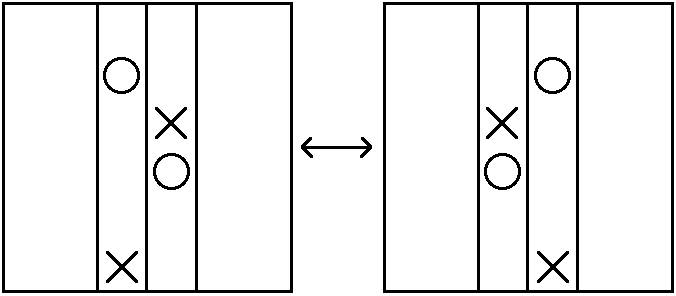
Figure 2. Commutation.

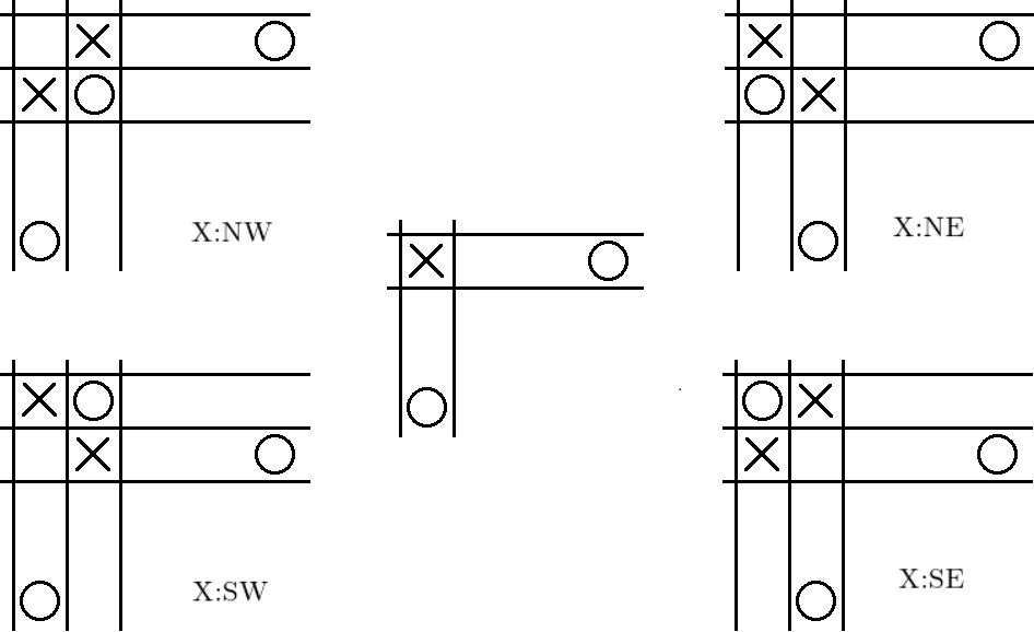
Figure 3. There are four types of stabilization.

In this paper, we only consider grid diagrams representing a knot.

2.2. Grid chain complexes

Let $\mathbb{G}$ be an $n\times n$ grid diagram. A state $\mathbf{x}$ of $\mathbb{G}$ is an $n$-tuple of points on the torus such that each horizontal circle $\alpha_{i}$ has exactly one point and each vertical circle $\beta_{j}$ has exactly one point of $\mathbf{x}$. We denote by $\mathbf{S}(\mathbb{G})$ the set of states of $\mathbb{G}$. For $\mathbf{x,y}\in\mathbf{S}(\mathbb{G})$, a domain $p$ from $\mathbf{x}$ to $\mathbf{y}$ is a formal linear combination of the closures of the squares in $\mathbb{G}\setminus(\boldsymbol{\alpha}\cup\boldsymbol{\beta})$ such that $\partial(\partial_{\alpha}p)=\mathbf{y}-\mathbf{x}$ and $\partial(\partial_{\beta}p)=\mathbf{x}-\mathbf{y}$, where $\partial_{\alpha}p$ is the portion of the boundary of $p$ in the horizontal circles $\alpha_{1}\cup\dots\cup\alpha_{n}$ and $\partial_{\beta}p$ is the portion of the boundary of $p$ in the vertical ones. A domain $p$ is positive if the coefficient of any square is nonnegative. In this paper, we always consider positive domains such that there is at least one square whose coefficient is zero for each row and column. We often call such a positive domain non-periodic. Let $\pi^{+}(\mathbf{x,y})$ denote the set of such domains from $\mathbf{x}$ to $\mathbf{y}$. For two states $\mathbf{x,y\in S}(\mathbb{G})$ with $|\mathbf{x\cap y}|=n-2$, an rectangle $r\in\pi^{+}(\mathbf{x},\mathbf{y})$ is a domain such that $\partial r$ is the union of four segments. Let $\mathrm{Rect}(\mathbf{x,y})$ be the set of rectangles from $\mathbf{x}$ to $\mathbf{y}$. A rectangle $r\in\mathrm{Rect}(\mathbf{x,y})$ is empty if $\mathbf{x}\cap\mathrm{Int}(r)=\mathbf{y}\cap\mathrm{Int}(r)=\emptyset$. Let $\mathrm{Rect}^{\circ}(\mathbf{x,y})$ be the set of empty rectangles from $\mathbf{x}$ to $\mathbf{y}$. If $|\mathbf{x\cap y}|\neq n-2$, then we define $\mathrm{Rect}^{\circ}(\mathbf{x,y})=\emptyset$. For two domains $p_{1}\in\pi(\mathbf{x,y})$ and $p_{2}\in\pi(\mathbf{y,z})$, the composite domain $p_{1}*p_{2}$ is the domain from $\mathbf{x}$ to $\mathbf{z}$ such that the coefficient of each square is the sum of the coefficient of the square of $p_{1}$ and $p_{2}$. In this paper, a rectangle is called a square if its width and height are the same.

We denote the set of $O$-markings by $\mathbb{O}$ and the set of $X$-markings by $\mathbb{X}$. We will use the labeling of markings as $\{O_{i}\}_{i=1}^{n}$ and $\{X_{j}\}_{j=1}^{n}$.

A planar realization of a toroidal diagram $\mathbb{G}$ is a planar figure obtained by cutting it along some $\alpha_{i}$ and $\beta_{j}$ and putting it on $[0,n)\times[0,n)\subset\mathbb{R}^{2}$ in a natural way.

For two points $(a_{1},a_{2}),(b_{1},b_{2})\in\mathbb{R}^{2}$, we say $(a_{1},a_{2})<(b_{1},b_{2})$ if $a_{1}<b_{1}$ and $a_{2}<b_{2}$. For two sets of finitely points $A,B\subset\mathbb{R}^{2}$, let $\mathcal{I}(A,B)$ be the number of pairs $a\in A,b\in B$ with $a<b$ and let $\mathcal{J}(A,B)=(\mathcal{I}(A,B)+\mathcal{I}(B,A))/2$. We consider that $n$ points of states are on lattice point on $\mathbb{R}^{2}$ and each $O$- and $X$-marking is located at $(l+\frac{1}{2},m+\frac{1}{2})$ for some $l,m\in\{0,1,\dots,n-1\}$. We regard a state $\mathbf{x}\in\mathbf{S}(\mathbb{G})$ as a set of $n$ lattice points in $[0,n)\times[0,n)\subset\mathbb{R}^{2}$.

Definition 2.1.

Take a planar realization of $\mathbb{G}$. For $\mathbf{x\in S}(\mathbb{G})$, the Maslov grading $M(\mathbf{x})$ and the Alexander grading $A(\mathbf{x})$ are defined by

(2.1) $$M(\mathbf{x}) =\mathcal{J}(\mathbf{x}-\mathbb{O},\mathbf{x}-\mathbb{O})+1,$$

(2.2) $$A(\mathbf{x}) =\mathcal{J}(\mathbf{x},\mathbb{X}-\mathbb{O})+\frac{1}{2}\mathcal{J}(\mathbb{O}+\mathbb{X},\mathbb{O}-\mathbb{X})-\frac{n-1}{2}.$$

Both the Maslov grading and the Alexander grading are well-defined as a toroidal diagram [12, Lemma 2.4].

For a positive domain $D\in\pi^{+}(\mathbf{x},\mathbf{y})$ and $i=1,\dots,n$, let $O_{i}(D)$ be the coefficient of the square containing $O_{i}$ and let

$$|D\cap\mathbb{O}|=\sum_{i=1}^{n}O_{i}(D).$$

We define $|D\cap\mathbb{X}|$ in the same way. The Alexander grading satisfies

(2.3) $$A(\mathbf{x})-A(\mathbf{y})=|D\cap\mathbb{X}|-|D\cap\mathbb{O}|.$$

for any $\mathbf{x,y\in S}(\mathbb{G})$ and $D\in\pi^{+}(\mathbf{x},\mathbf{y})$ [18, Proposition 4.3.3].

Definition 2.2.

Let $\widetilde{GC}_{d}(\mathbb{G},s)$ be the $\mathbb{F}$-vector space generated by the states whose the Maslov grading is $d$ and the Alexander grading is $s$. The (tilde) grid chain complex is the bigraded $\mathbb{F}$-vector space $\widetilde{GC}(\mathbb{G})=\bigoplus_{d,s\in\mathbb{Z}}\widetilde{GC}_{d}(\mathbb{G},s)$ whose differential is defined by

$$\partial(\mathbf{x})=\sum_{\mathbf{y}}\#\{\\ r\in\mathrm{Rect}^{\circ}(\mathbf{x},\mathbf{y})|r\cap\mathbb{O}=r\cap\mathbb{X}=\emptyset\}\cdot\mathbf{y},$$

where $\#\{\cdot\}$ counts modulo two. The homology of $\widetilde{GC}(\mathbb{G})$ is denoted by $\widetilde{GH}(\mathbb{G})$.

Proposition 2.3 ([12, Proposition 2.9]).

The grid chain complex $\widetilde{GC}(\mathbb{G})$ is a bigraded chain complex, i.e., the differential $\partial$ satisfies $\partial\circ\partial=0$, drops the Maslov grading by one, and preserves the Alexander grading.

Let $W$ be a two-dimensional graded vector space $W\cong\mathbb{F}_{0,0}\oplus\mathbb{F}_{-1,-1}$. For a bigraded $\mathbb{F}$-vector space $X$, the shift of $X$, denoted $X\llbracket a,b\rrbracket$, is the bigraded $\mathbb{F}$-vector space so that $X\llbracket a,b\rrbracket_{d,s}=X_{d+a,s+b}$. Then, we have

$$X\otimes W\cong X\oplus X\llbracket 1,1\rrbracket.$$

Theorem 2.4 ([12, Theorem 1.2, Proposition 2.15]).

For an $n\times n$ grid diagram representing a knot $K$, let $\widehat{GH}(\mathbb{G})$ be the bigraded vector space defined by

$$\widetilde{GH}(\mathbb{G})\cong\widehat{GH}(\mathbb{G})\otimes W^{\otimes(n-1)}.$$

Then $\widehat{GH}(\mathbb{G})$ is a knot invariant.

Remark 2.5.

Originally, the hat grid homology $\widehat{GH}(\mathbb{G})$ is defined in a different way. The minus grid chain complex $GC^{-}(\mathbb{G})$ is first defined and then the hat complex $\widehat{GC}(\mathbb{G})$ is defined as the quotient complex of $GC^{-}(\mathbb{G})$. See [12] or [18].

3. The top term of grid homology

Definition 3.1.

For an $n\times n$ grid diagram $\mathbb{G}$, let $\mathbf{x}_{0}(\mathbb{G})$ be the state of $\mathbb{G}$ consisting of northwest corners of the squares containing an $O$-marking (Figure 4).

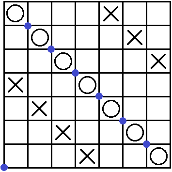
Figure 4. The state $\mathbf{x}_{0}(\mathbb{G})$

Proposition 3.2.

If $\mathbb{G}$ is a diagonal grid diagram representing a knot, then $A(\mathbf{x})<A(\mathbf{x}_{0}(\mathbb{G}))$ if $\mathbf{x}\neq\mathbf{x}_{0}(\mathbb{G})$.

We consider a planar realization of a $n\times n$ grid diagram $\mathbb{G}$ in $[0,n)\times[0,n)\subset\mathbb{R}^{2}$. The winding matrix of $\mathbb{G}$ is the $n\times n$ matrix $\mathbf{W}(\mathbb{G})=(a_{i\,j})$ where $a_{i\,j}$ is $(-1)$ times the winding number of the lattice point $c_{i\,j}=(j-1,n-i)$ (Figure 5), i.e.,

(3.1) $$a_{i\,j}=\mathcal{J}(\{c_{i\,j}\},\mathbb{X}-\mathbb{O}).$$

By (2.2), the Alexander grading of a state $\mathbf{x}=(x_{i})_{i=1}^{n}$ of $\mathbb{G}$ is the sum of $(-1)$ times the winding numbers of $x_{i}$’s and some constant $C=C(\mathbb{G})$.

Lemma 3.3.

Suppose that $\mathbb{G}$ is a diagonal grid diagram representing a knot $K$. Let $\mathbf{W}(\mathbb{G})=(a_{i\,j})$ be the winding matrix of $\mathbb{G}$. Then we have $a_{i\,j}\geq 0$ for any $i,j$ and $a_{i\,i+1}\geq 1$ for $i=1,\dots,n-1$.

Proof.

Since the entry $a_{i\,j}$ is $(-1)$ times the winding number of the lattice point $(j-1,n-i)\in[0,n)\times[0,n)$, $a_{i\,j}=0$ if $i=n$. If the lattice point corresponding to an entry $a_{i\,j}$ is above the line $y=-x+n$, consider the ray from the lattice point to the right. Since vertical segments (connecting an $O$-marking and an $X$-marking) that meet the ray are downward, we have $a_{i\,j}\geq 0$. If the lattice point corresponding to an entry $a_{i\,j}$ is below the line $y=-x+n$, draw the ray from the lattice point to the left. Then we have $a_{i\,j}\geq 0$ in the same way. Now we consider that the lattice point corresponding to $a_{i\,j}$ is on the line $y=-x+n$, in other words, $j=i+1$. Since the lattice point is sandwiched by the two $O$-markings and all of the $O$-markings are on the diagonal, Equation (3.1) is just

$$a_{i\,i+1} =\#\{X|X\text{ is on the right above the point }(i,n-i)\}$$

$$=\#\{X|X\text{ is lower left than the point }(i,n-i)\}.$$

The second equality is because the number of the $X$-markings under $a_{i\,i+1}$ and the number of the $X$-markings that are to the right of $a_{i\,i+1}$ are the same. If $a_{i\,i+1}=0$ and $i<n-1$, then obviously $\mathbb{G}$ represents a split link. If $a_{i\,i+1}=0$ and $i=n-1$, then $\mathbb{G}$ does not contain an $X$-marking in the rightmost column. Therefore $a_{i\,i+1}\geq 1$ for $i=1,\dots,n-1$ ∎

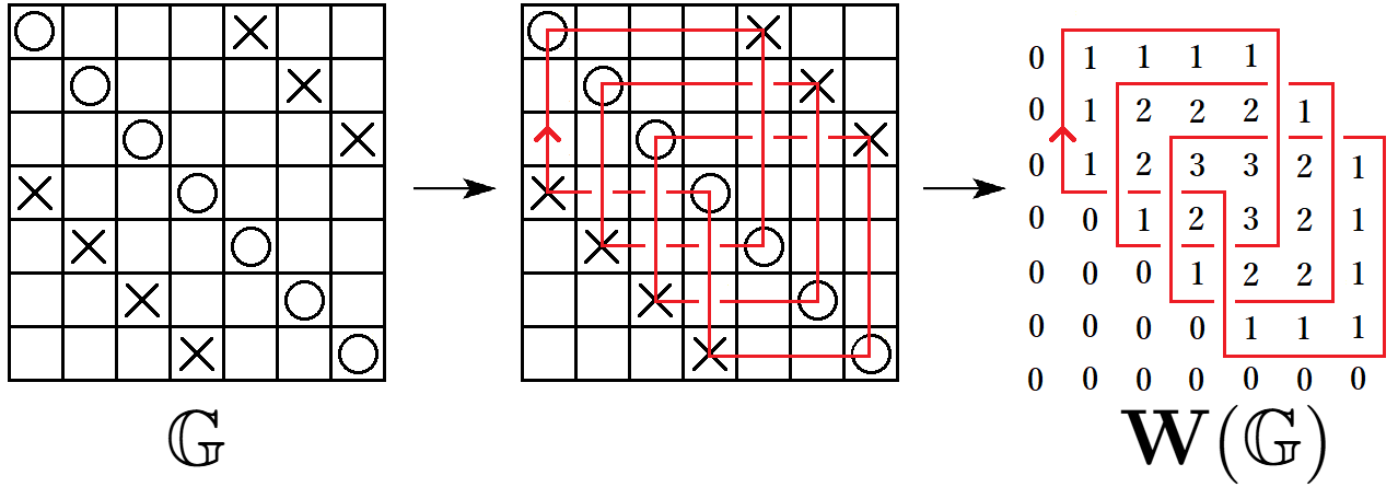
Figure 5. A grid diagram $\mathbb{G}$ and its winding matrix $\mathbf{W}(\mathbb{G})$.

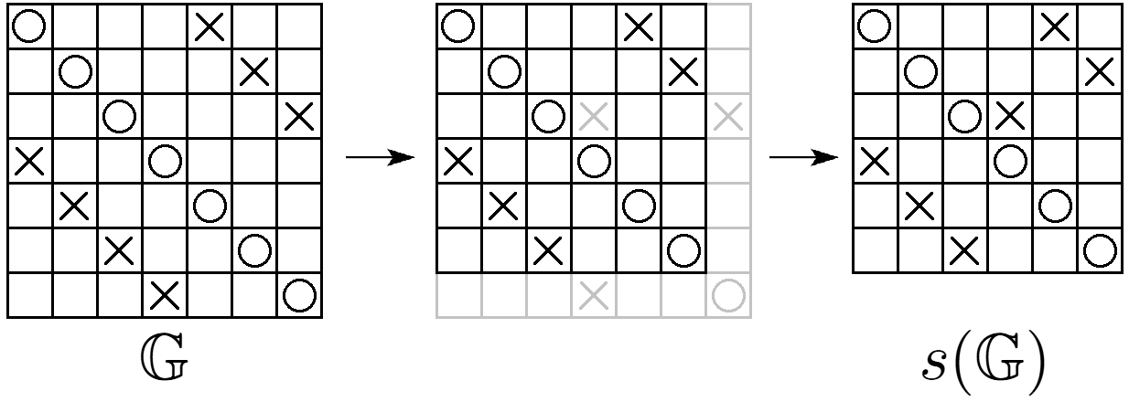
Figure 6. An example of $\mathbb{G}$ and $s(\mathbb{G})$.

$$\mathbf{W}(\mathbb{G})=\hskip 30.0pt \mathbf{W}^{\prime}(\mathbb{G})=\hskip 30.0pt \mathbf{W}(s(\mathbb{G}))=\hskip 20.0pt$$

(3.2) $$\begin{pmatrix}0&1&1&1&1&0&0\\ 0&1&2&2&2&1&0\\ 0&1&2&3&3&2&1\\ 0&0&1&2&3&2&1\\ 0&0&0&1&2&2&1\\ 0&0&0&0&1&1&1\\ 0&0&0&0&0&0&0\end{pmatrix} \longrightarrow \begin{pmatrix}0&1&1&1&1&0&0\\ 0&1&2&2&2&1&0\\ 0&1&2&3&{\color[rgb]{1,0,0}2}&{\color[rgb]{1,0,0}1}&{\color[rgb]{1,0,0}0}\\ 0&0&1&2&{\color[rgb]{1,0,0}2}&{\color[rgb]{1,0,0}1}&{\color[rgb]{1,0,0}0}\\ 0&0&0&1&{\color[rgb]{1,0,0}1}&{\color[rgb]{1,0,0}1}&{\color[rgb]{1,0,0}0}\\ 0&0&0&0&{\color[rgb]{1,0,0}0}&{\color[rgb]{1,0,0}0}&{\color[rgb]{1,0,0}0}\\ 0&0&0&0&0&0&0\end{pmatrix} \longrightarrow \begin{pmatrix}0&1&1&1&1&0\\ 0&1&2&2&2&1\\ 0&1&2&3&{\color[rgb]{1,0,0}2}&{\color[rgb]{1,0,0}1}\\ 0&0&1&2&{\color[rgb]{1,0,0}2}&{\color[rgb]{1,0,0}1}\\ 0&0&0&1&{\color[rgb]{1,0,0}1}&{\color[rgb]{1,0,0}1}\\ 0&0&0&0&0&0\\ \end{pmatrix}$$

Proof of Proposition 3.2.

We will prove by induction on the size of grid diagram $n$.

The case $n=2$ is easy.

Suppose that Proposition 3.2 holds for any $(n-1)\times(n-1)$ diagonal grid diagram representing a knot.

Let $\mathbb{G}$ be an $n\times n$ diagonal grid diagram representing a knot. We regard a state $\mathbf{x}$ as a set of $n$ lattice points $\mathbf{x}=\{x_{1},\dots,x_{n}\}$ in $[0,n)\times[0,n)$. Then we have that

$$A(\mathbf{x})>A(\mathbf{x}^{\prime})\text{ if and only if }\sum_{i}w(x_{i})>\sum_{i}w(x_{i}^{\prime}).$$

Let $A^{\prime}(\mathbf{x})=\sum_{i}w(x_{i})$. The winding number $w(x_{i})$ equals the entry of $\mathbf{W}(\mathbb{G})$ corresponding to the lattice point $x_{i}$.

Let $O_{n}$ be the $O$-marking in the rightmost column. Let $s(\mathbb{G})$ be the $(n-1)\times(n-1)$ grid diagram obtained from $\mathbb{G}$ by removing the row and column containing $O_{n}$ and adding an $X$-marking (Figure 6). If $\mathbb{G}$ is a diagonal grid diagram representing a knot, then so is $s(\mathbb{G})$. Let $X_{k}$ be the $X$-marking in the bottom row and $X_{n}$ be the $X$-marking in the rightmost column. Suppose that the $x$-coordinate of $X_{k}$ is $n_{x}-1/2$ and the $y$-coordinate of $X_{n}$ is $n_{y}-1/2$. Let $\mathbf{W}^{\prime}(\mathbb{G})$ is the $n\times n$ matrix obtained from $\mathbf{W}(\mathbb{G})$ by subtracting one from $a_{ij}$ for $j>n_{x}$ and $n-n_{y}<i<n$. Then the winding matrix $\mathbf{W}(s(\mathbb{G}))$ is obtained from $\mathbf{W}^{\prime}(\mathbb{G})$ by removing the rightmost column and the $(n-1)$-th row. Let $m=\min\{n-n_{x},n_{y}-1\}$. For example, if $\mathbb{G}$ is the $7\times 7$ grid diagram as in Figure 6, then $\mathbf{W}(\mathbb{G})$ is in the left of (3.2). Because the red area of $\mathbf{W}^{\prime}(\mathbb{G})$ has a width of $3$ and a height of $4$, we have $m=3$.

Write $\mathbf{W}(\mathbb{G})=(a_{i\,j})$, $\mathbf{W}^{\prime}(\mathbb{G})=(b_{i\,j})$, and $\mathbf{W}(s(\mathbb{G}))=(c_{i\,j})$. Then $A^{\prime}(\mathbf{x}_{0}(\mathbb{G}))=a_{n\,1}+a_{1\,2}+a_{2\,3}+\dots+a_{n-1\,n}$. By the relation between $\mathbf{W}(\mathbb{G})$ and $\mathbf{W}(s(\mathbb{G}))$, we have

(3.3) $$A^{\prime}(\mathbf{x}_{0}(s(\mathbb{G})))=A^{\prime}(\mathbf{x}_{0}(\mathbb{G}))-m.$$

Let $\mathbf{x}$ be a state of $\mathbb{G}$ such that $\mathbf{x}\neq\mathbf{x}_{0}(\mathbb{G})$. It is sufficient to prove $A^{\prime}(\mathbf{x})<A^{\prime}(\mathbf{x}_{0}(\mathbb{G}))$. Write $A^{\prime}(\mathbf{x})=a_{i_{1}\,1}+\dots+a_{i_{n}\,n}$. Then by the definition of $\mathbf{W}^{\prime}(\mathbb{G})$, we have

(3.4) $$A^{\prime}(\mathbf{x})-m\leq b_{i_{1}\,1}+\dots+b_{i_{n}\,n}.$$

We will consider the state of $s(\mathbb{G})$ determined by $\mathbf{x}$. There are two cases.

1. If $i_{n}=n-1$, let $i_{k}=n$. The state $\mathbf{x}$ naturally determines a state $s(\mathbf{x})\in\mathbf{S}(s(\mathbb{G}))$ by deleting $a_{i_{n}\,n}$. The entries $\{c_{i_{1}\,1},\dots,c_{i_{n-1}\,n-1}\}\cup\{c_{i_{k}-1\,k}\}\setminus\{c_{i_{k}\,k}\}$ of $\mathbf{W}(s(\mathbb{G}))$ correspond to $s(\mathbf{x})$. We have

   (3.5) $$c_{i_{1}\,1}+\dots+c_{i_{k-1}\,k-1}+c_{i_{k}-1\,k}+c_{i_{k+1}\,k+1}+\dots+c_{i_{n-1}\,n-1}=b_{i_{1}\,1}+\dots+b_{i_{n}\,n}.$$

   Obviously, $s(\mathbf{x})\neq\mathbf{x}_{0}(s(\mathbb{G}))$ (Figure 7). By the induction hypothesis, we have

   (3.6) $$c_{i_{1}\,1}+\dots+c_{i_{k-1}\,k-1}+c_{i_{k}-1\,k}+c_{i_{k+1}\,k+1}+\dots+c_{i_{n-1}\,n-1}<A^{\prime}(\mathbf{x}_{0}(s(\mathbb{G}))).$$

   Equations (3.3)-(3.6) imply $A^{\prime}(\mathbf{x})<A^{\prime}(\mathbf{x}_{0}(\mathbb{G}))$

2. If $i_{n}\neq n-1$, let $i_{k}=n$ and $i_{l}=n-1$. The state $s(\mathbf{x})\in\mathbf{S}(s(\mathbb{G}))$ is obtained from $\mathbf{x}$ by two steps: First, we take a new state of $\mathbb{G}$ containing $a_{n-1\,n}$ by deleting the entries $a_{n-1\,l}$ and $a_{i_{n}\,n}$ and adding $a_{i_{n}\,l}$ and $a_{n-1\,n}$. Then the same procedure as above gives $s(\mathbf{x})$. Then we have

   (3.7) $$c_{i_{1}\,1}+\dots+c_{i_{k}-1\,k}+\dots+c_{i_{n}\,l}+\dots+c_{i_{n-1}\,n-1}\geq b_{i_{1}\,1}+\dots+b_{i_{n}\,n}$$

   because of Lemma 3.3 and that $b_{i_{l}\,l}=b_{i_{n}\,n}=0$. The entries on the left side of (3.7) represent a state $s(\mathbf{x})$.

   1. If $s(\mathbf{x})\neq\mathbf{x}_{0}(s(\mathbb{G}))$, then the same argument as the previous case implies $A^{\prime}(\mathbf{x})<A^{\prime}(\mathbf{x}_{0}(\mathbb{G}))$ (Figure 8).

   2. If $s(\mathbf{x})=\mathbf{x}_{0}(s(\mathbb{G}))$, then (3.7) is modified as

      (3.8) $$c_{i_{1}\,1}+\dots+c_{i_{k}-1\,k}+\dots+c_{i_{n}\,l}+\dots+c_{i_{n-1}\,n-1}\geq b_{i_{1}\,1}+\dots+b_{i_{n}\,n}+1.$$

      because $b_{i_{l}\,l}=b_{i_{n}\,n}=b_{n-1\,n}=0$ and $b_{i_{n}\,l}\geq 1$ (Lemma 3.3). Furthermore, we have

      (3.9) $$c_{i_{1}\,1}+\dots+c_{i_{k}-1\,k}+\dots+c_{i_{n}\,l}+\dots+c_{i_{n-1}\,n-1}=A^{\prime}(\mathbf{x}_{0}(s(\mathbb{G})))$$

      since $s(\mathbf{x})=\mathbf{x}_{0}(s(\mathbb{G}))$ (Figure 9). Now we have $A^{\prime}(\mathbf{x})\leq A^{\prime}(\mathbf{x}_{0}(\mathbb{G}))-1$ and thus $A^{\prime}(\mathbf{x})<A^{\prime}(\mathbf{x}_{0}(\mathbb{G}))$.

∎

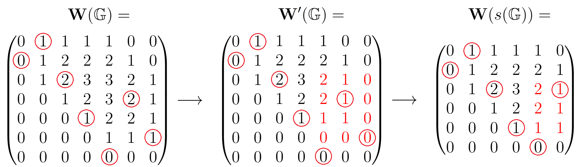
Figure 7. A process to obtain a state of $s(\mathbb{G})$ from a state of $\mathbb{G}$ in the case i.

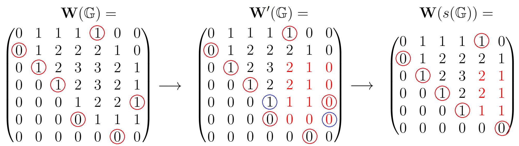
Figure 8. A process to obtain a state of $s(\mathbb{G})$ from a state of $\mathbb{G}$ in the case ii1.

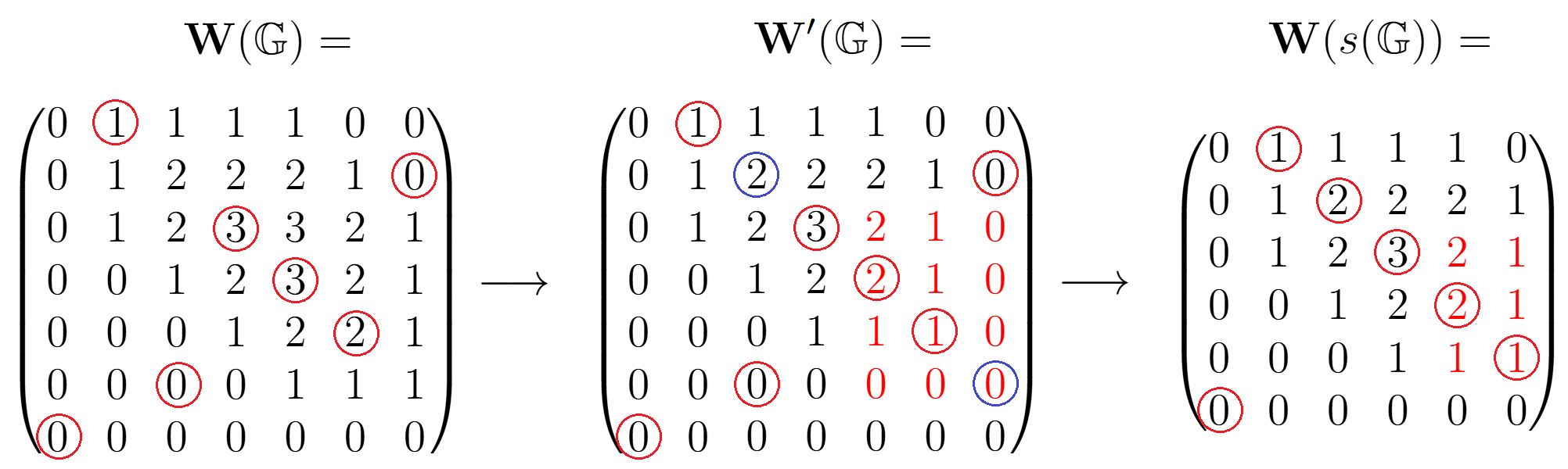
Figure 9. A process to obtain a state of $s(\mathbb{G})$ from a state of $\mathbb{G}$ in the case ii2.

Proof of Equation (1.1) in Theorem 1.8.

This follows from Proposition 3.2. ∎

4. The next-to-top term of grid homology

Proof of Equation (1.2) in Theorem 1.8.

Let $\mathbb{G}$ be an $n\times n$ diagonal grid diagram representing a prime diagonal knot $K$. By applying grid moves to $\mathbb{G}$, we can assume that

1. No square containing an $X$-marking share an edge with any square containing an $O$-marking, and

2. $\mathbb{G}$ is the smallest among diagonal grid diagrams representing $K$.

We recall that the state $\mathbf{x}_{0}=\mathbf{x}_{0}(\mathbb{G})$ (Definition 3.1) satisfies $A(\mathbf{x})<A(\mathbf{x}_{0})$ if $\mathbf{x}\neq\mathbf{x}_{0}$. Let $\mathbf{x}_{1},\dots,\mathbf{x}_{n}$ be the states obtained from $\mathbf{x}_{0}$ by switching the height of adjacent two points.

To prove the Theorem, we will see

$$(M(\mathbf{x}_{i}),A(\mathbf{x}_{i}))=(M(\mathbf{x}_{0})-1,A(\mathbf{x}_{0})-1)$$

for $i=1,\dots,n$, and $A(\mathbf{x})\leq A(\mathbf{x}_{0})-2$ if $\mathbf{x}\neq\mathbf{x}_{0},\mathbf{x}_{1},\dots,\mathbf{x}_{n}$. If this is verified, then the grid homology $\widetilde{GH}(\mathbb{G})$ with the Alexander grading $A(\mathbf{x}_{0})-1=g(K)-1$ is

$$\widetilde{GH}_{d}(\mathbb{G},g(K)-1)\cong\begin{cases}\mathbb{F}^{n}&d=M(\mathbf{x}_{0})-1\\ 0&d\neq M(\mathbf{x}_{0})-1.\end{cases}$$

Then Theorem 2.4 concludes the proof.

Let $\mathbf{x}$ be a state with $\mathbf{x}\neq\mathbf{x}_{0}$. There are positive domains from $\mathbf{x}$ to $\mathbf{x}_{0}$ that are non-periodic. Any such a domain $D\in\pi^{+}(\mathbf{x},\mathbf{x}_{0})$ satisfies (2.3). It is sufficient to prove that if $A(\mathbf{x})=A(\mathbf{x}_{0})-1$, the domain $D$ must be a single $1\times 1$ or $(n-1)\times(n-1)$ square. Let $m=\#(\mathbf{x}_{0}\cap D)$ be the number of $90^{\circ}$ or $270^{\circ}$ corners of $D$ coming from $\mathbf{x}_{0}$. A $90^{\circ}$ corner of $\mathbf{x}_{0}\cap D$ is the northwest or southeast corner of $D$.

First, we consider the case when $m=2$, in other words, the domain $D$ is a square (possibly larger than a $1\times 1$ square). We will see that for any square $D\in\pi^{+}(\mathbf{x},\mathbf{x}_{0})$ for some state $\mathbf{x}$, we have

(4.1) $$|D\cap\mathbb{O}|-|D\cap\mathbb{X}|=\begin{cases}1&\text{if $D$ is a $1\times 1$ or $(n-1)\times(n-1)$ square}\\ >1&\text{otherwise}.\end{cases}$$

Since there are exactly two squares $D$ and $D^{\prime}$ from $\mathbf{x}$ to $\mathbf{x}_{0}$ (both satisfy Equation (2.3)), we can assume that $D$ is the smaller one. Let $D$ be a $l\times l$ square.

1. If $l=1$, obviously we have $|D\cap\mathbb{O}|-|D\cap\mathbb{X}|=1$.

2. If $l=2$, by assumption (A), the square $D$ must contain two $O$-markings but no $X$-marking. Therefore we have $|D\cap\mathbb{O}|-|D\cap\mathbb{X}|=2$.

3. If $l=3$, suppose that $|D\cap\mathbb{O}|-|D\cap\mathbb{X}|=1$. By assumption (A), $\mathbb{G}$ represents a link with more than one component (Figure 10). This contradicts our assumption that $\mathbb{G}$ represents a knot.

4. If $l>3$, consider a new $(l+1)\times(l+1)$ diagonal grid diagram $\mathbb{G}(D)$ obtained from $D$ by adding one row and column and putting one $O$-marking and two $X$-markings (Figure 11). By assumption (B), the diagram $\mathbb{G}(D)$ does not represent the unknot. By the same argument, the $(n-l+1)\times(n-l+1)$ grid diagram $\mathbb{G}(D^{\prime})$ obtained from $D^{\prime}$ in the same way also does not represent the unknot. This contradicts our assumption that $\mathbb{G}$ represents a prime knot.

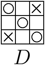
Figure 10. A $3\times 3$ square $D$ appearing in the case (3).

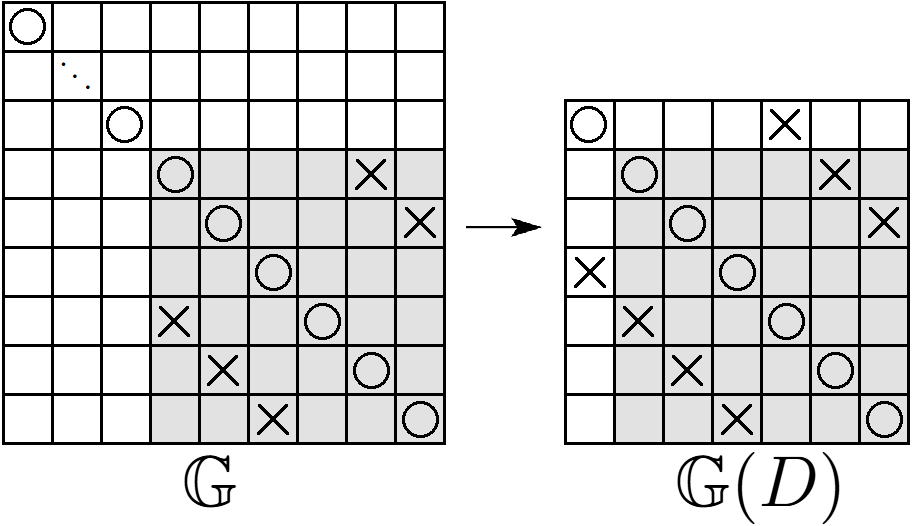
Figure 11. A square $D$ (gray area) in $\mathbb{G}$ and a resulting diagram $\mathbb{G}(D)$ in the case (4).

Next, we will consider the case $m>2$. For any domain $D\in\pi^{+}(\mathbf{x},\mathbf{x}_{0})$, there is a positive domain $E\in\pi^{+}(\mathbf{y},\mathbf{x})$ such that the composite domain $D^{\prime}=E*D$ is the sum of square domains two of whose corners are the points of $\mathbf{x}_{0}$ (Figure 12). Since $m>2$, $D^{\prime}$ consists of more than one square or is a square larger than $1\times 1$ and smaller than $(n-1)\times(n-1)$. Since the diagonal of each square consisting of $D^{\prime}$ is on the diagonal of $\mathbb{G}$, we can apply Equation (4.1) to $D^{\prime}$. Then we have

$$|D^{\prime}\cap\mathbb{O}|-|D^{\prime}\cap\mathbb{X}|>1.$$

By the construction of $D^{\prime}$, we have $|D\cap\mathbb{O}|=|D^{\prime}\cap\mathbb{O}|$ and $|D\cap\mathbb{X}|\leq|D^{\prime}\cap\mathbb{X}|$. Therefore we have

$$|D\cap\mathbb{O}|-|D\cap\mathbb{X}|\geq|D^{\prime}\cap\mathbb{O}|-|D^{\prime}\cap\mathbb{X}|>1.$$

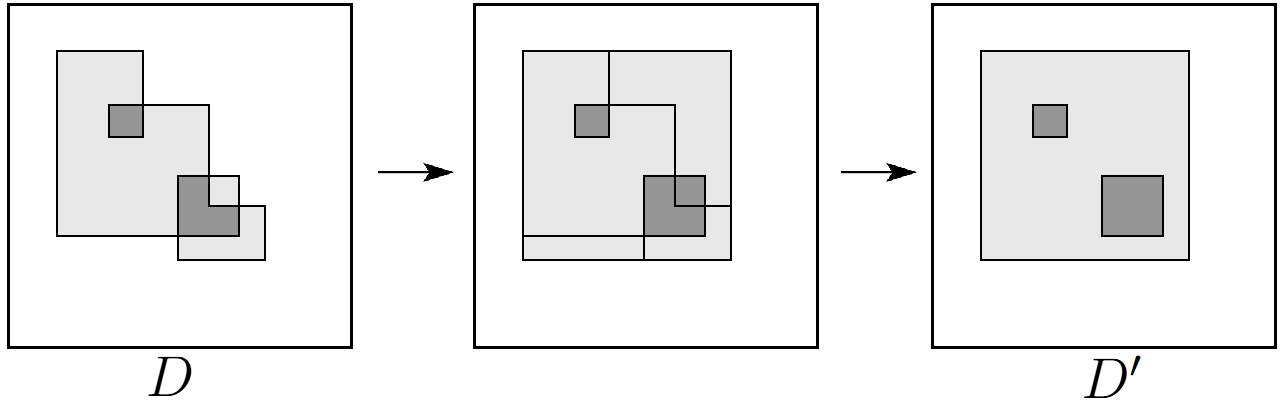
Figure 12. An example of domains $D$ and $D^{\prime}$. The coefficients of squares are one in light gray regions and two in gray regions.

∎

Appendix A Diagonal grid diagrams for some positive braids

We give diagonal grid diagrams for some positive braid knots. By rotating a braid $90^{\circ}$ clockwise, we can easily get a grid diagram representing the closure of a braid. We remark that if a grid diagram represents an oriented link $\vec{L}$, then its reflection across the diagonal represents $-\vec{L}$, where $-\vec{L}$ is the orientation reversing of $\vec{L}$. Figure 13 shows the procedure to obtain a diagonal grid diagram representing the knot $10_{139}$.

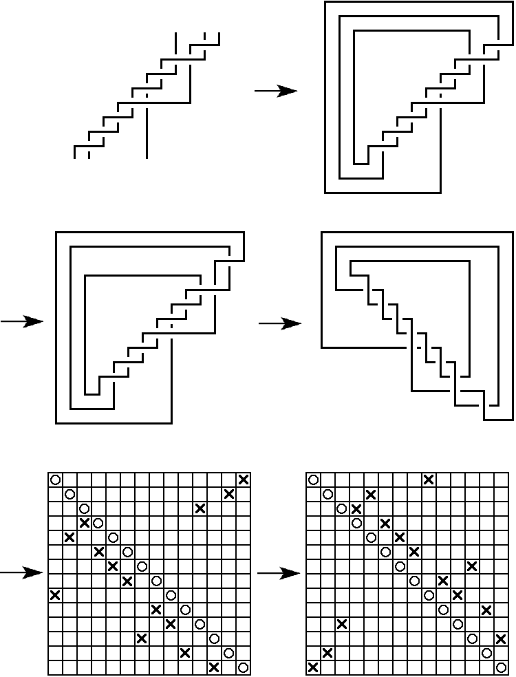
Figure 13. A diagonal grid diagram representing the knot $10_{139}$ which is the closure of the braid $\sigma_{1}^{4}\sigma_{2}\sigma_{1}^{3}\sigma_{2}^{2}$. The grid diagrams in the bottom left and bottom right represent $-10_{139}$ and $10_{139}$ respectively.

Proposition A.1.

Let $[m]=\sigma_{1}^{m}\sigma_{2}\in\mathcal{B}_{3}$ be the word of the braid group (Figure 14). If a link has a braid representation as $[m_{1}]\dots[m_{i}]\sigma_{2}^{l}$ for some positive integers $m_{1},\dots,m_{i}$ and non-negative integer $l$, then there exists a diagonal grid diagram representing it.

Proof.

This immediately follows from the idea of the above procedure (See Figure 15). ∎

By this Proposition, the knots

$$10_{139},12n_{i}\ (i=242,472,574,725),14n_{j}\ (j=6022,12201,15856,18079,21324,24551)$$

that are not torus knots are diagonal. Prime positive braid knots with the genus up to $6$ are in [9]. See also [2]. We remark that the knot $12n_{242}$ is an $L$-space knot and $12n_{472}$, $12n_{574}$, and $12n_{725}$ are not.

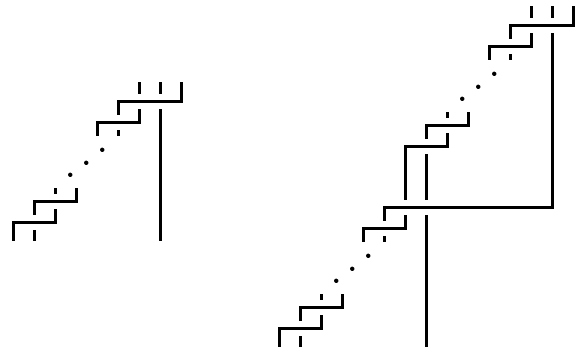
Figure 14. Left: the braid $[m]:=\sigma_{1}^{m}\sigma_{2}$. Right: the composite braid $[m][m^{\prime}]$.

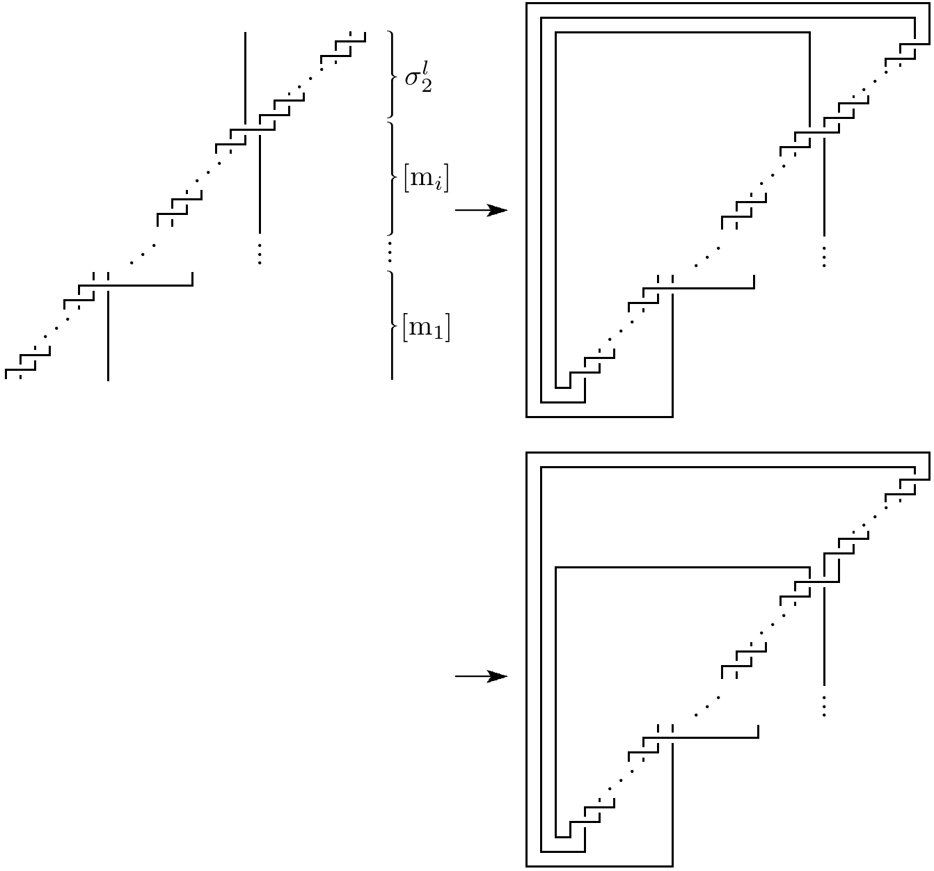
Figure 15. The positive braid $[m_{1}]\dots[m_{i}]\sigma_{2}^{l}$ and its closure $L$.

References

- [1] Jackson Arndt, Malia Jansen, Payton McBurney, and Katherine Vance, Diagonal knots and the tau invariant, arXiv:2412.13796, 2025.
- [2] Sebastian Baader, Lukas Lewark, and Livio Liechti, Checkerboard graph monodromies, Enseign. Math. 64 (2018), no. 1-2, 65–88. MR 3959848
- [3] Joan Birman and Ilya Kofman, A new twist on Lorenz links, J. Topol. 2 (2009), no. 2, 227–248. MR 2529294
- [4] Joan S. Birman, Lorenz knots, arXiv:1201.0214, 2011.
- [5] Peter R. Cromwell, Embedding knots and links in an open book. I. Basic properties, Topology Appl. 64 (1995), no. 1, 37–58. MR 1339757
- [6] Paolo Ghiggini, Knot Floer homology detects genus-one fibred knots, Amer. J. Math. 130 (2008), no. 5, 1151–1169. MR 2450204
- [7] Matthew Hedden, Notions of positivity and the Ozsváth-Szabó concordance invariant, J. Knot Theory Ramifications 19 (2010), no. 5, 617–629. MR 2646650
- [8] Tetsuya Ito, A note on HOMFLY polynomial of positive braid links, Internat. J. Math. 33 (2022), no. 4, Paper No. 2250031, 18. MR 4402791
- [9] Lukas Lewark, Lukas lewark, https://people.math.ethz.ch/~llewark/braids.php.
- [10] Charles Livingston and Allison H. Moore, Knotinfo: Table of knot invariants, https://knotinfo.math.indiana.edu/index.php.
- [11] Ciprian Manolescu, Peter Ozsváth, and Sucharit Sarkar, A combinatorial description of knot Floer homology, Ann. of Math. (2) 169 (2009), no. 2, 633–660. MR 2480614
- [12] Ciprian Manolescu, Peter Ozsváth, Zoltán Szabó, and Dylan Thurston, On combinatorial link Floer homology, Geom. Topol. 11 (2007), 2339–2412. MR 2372850
- [13] John Milnor, Singular points of complex hypersurfaces, Annals of Mathematics Studies, vol. No. 61, Princeton University Press, Princeton, NJ; University of Tokyo Press, Tokyo, 1968. MR 239612
- [14] Yi Ni, Knot Floer homology detects fibred knots, Invent. Math. 170 (2007), no. 3, 577–608. MR 2357503
- [15] by same author, The next-to-top term in knot Floer homology, Quantum Topol. 13 (2022), no. 3, 579–591. MR 4537314
- [16] Peter Ozsváth and Zoltán Szabó, Holomorphic disks and knot invariants, Adv. Math. 186 (2004), no. 1, 58–116. MR 2065507
- [17] Peter Ozsváth and Zoltán Szabó, On knot Floer homology and lens space surgeries, Topology 44 (2005), no. 6, 1281–1300. MR 2168576
- [18] Peter S. Ozsváth, András I. Stipsicz, and Zoltán Szabó, Grid homology for knots and links, Mathematical Surveys and Monographs, vol. 208, American Mathematical Society, Providence, RI, 2015. MR 3381987
- [19] R. V. Razumovskiĭ, Some classes of fibered links, Sibirsk. Mat. Zh. 55 (2014), no. 4, 840–850. MR 3242599
- [20] Roman Razumovsky, Grid diagrams of Lorenz links, J. Knot Theory Ramifications 19 (2010), no. 6, 843–847. MR 2665773
- [21] Sucharit Sarkar, Grid diagrams and the Ozsváth-Szabó tau-invariant, Math. Res. Lett. 18 (2011), no. 6, 1239–1257. MR 2915478
- [22] John R. Stallings, Constructions of fibred knots and links, Algebraic and geometric topology (Proc. Sympos. Pure Math., Stanford Univ., Stanford, Calif., 1976), Part 2, Proc. Sympos. Pure Math., vol. XXXII, Amer. Math. Soc., Providence, RI, 1978, pp. 55–60. MR 520522
- [23] Alexander Stoimenow, Knot data tables, http://stoimenov.net/stoimeno/homepage/ptab/.