Robust Reward Alignment via Hypothesis Space Batch Cutting

Abstract

Reward design for reinforcement learning and optimal control agents is challenging. Preference-based alignment addresses this by enabling agents to learn rewards from ranked trajectory pairs provided by humans. However, existing methods often struggle from poor robustness to unknown false human preferences. In this work, we propose a robust and efficient reward alignment method based on a novel and geometrically interpretable perspective: hypothesis space batched cutting. Our method iteratively refines the reward hypothesis space through “cuts” based on batches of human preferences. Within each batch, human preferences, queried based on disagreement, are grouped using a voting function to determine the appropriate cut, ensuring a bounded human query complexity. To handle unknown erroneous preferences, we introduce a conservative cutting method within each batch, preventing erroneous human preferences from making overly aggressive cuts to the hypothesis space. This guarantees provable robustness against false preferences. We evaluate our method in a model predictive control setting across diverse tasks, including DM-Control, dexterous in-hand manipulation, and locomotion. The results demonstrate that our framework achieves comparable or superior performance to state-of-the-art methods in error-free settings while significantly outperforming existing method when handling high percentage of erroneous human preferences.

1 Introduction

Reinforcement learning and optimal control have shown great success in generating intricate behavior of an agent/robot, such as dexterous manipulation (Qi et al., 2023; Handa et al., 2023; Yin et al., 2023) and agile locomotion (Radosavovic et al., 2024; Tsounis et al., 2020; Hoeller et al., 2024). In these applications, reward/cost functions are essential, as they dictate agent behavior by rewarding/penalizing different aspects of motion in a balanced manner. However, designing different reward terms and tuning their relative weights is nontrivial, often requiring extensive domain knowledge and laborious trial-and-error. This is further amplified in user-specific applications, where agent behavior must be tuned to align with individual user preferences.

Reward alignment automates reward design by enabling an agent to learn its reward function directly from intuitive human feedback (Casper et al., 2023). In preference-based feedback, a human ranks a pair of the agent’s motion trajectories, and then the agent infers a reward function that best aligns with human judgment. Numerous alignment methods have been proposed (Christiano et al., 2017; Ibarz et al., 2018; Hejna III & Sadigh, 2023), with most relying on the Bradley-Terry model (Bradley & Terry, 1952), which formalizes the rationality of human preferences. While effective, these models are vulnerable to false human preferences, where rankings may be irrational or inconsistent due to human errors, mistakes, malicious interference, or difficulty distinguishing between equally undesirable trajectories. When a significant portion of human feedback is erroneous, the learned reward function degrades substantially, leading to poor agent behavior.

In this paper, we propose a robust reward alignment framework based on a novel and interpretable perspective: hypothesis space batch cutting. We maintain a hypothesis space of reward models during learning, where each batch of human preferences introduces a nonlinear cut, removing portions of the hypothesis space. Within each batch, human preferences, queried based on disagreement over the current hypothesis space, are grouped using a proposed voting function to determine the appropriate cut. This process ensures a certifiable upper bound on the number of human preferences required. To tackle false human preferences, we introduce a conservative cutting method within each batch. This prevents false human preferences from making overly aggressive cuts to the hypothesis space and ensures provable robustness. Extensive experiments demonstrate that our framework achieves comparable or superior performance to state-of-the-art methods in error-free settings while significantly outperforming existing approaches when handling high rates of erroneous human preferences.

2 Related Works

2.1 Preference-Based Reward Learning

Learning rewards from preferences falls in the category of learning utility functions in Preference-based Reinforcement Learning (PbRL) (Wirth et al., 2017), and was early studied in (Zucker et al., 2010; Akrour et al., 2012, 2014). In those early works, typically a set of weights for linear features is learned. With neural network representations, a scalable PbRL framework of learning reward is developed in (Christiano et al., 2017), recently used for fine tuning large language models (Bakker et al., 2022; Achiam et al., 2023). In those works, human preference is modelled using Bradley-Terry formulation (Bradley & Terry, 1952). Numerous variants of this framework have been developed (Hejna III & Sadigh, 2023; Hejna et al., 2023; Myers et al., 2022, 2023) over time. Recently, progress has been made to improve human data complexity. PEBBLE (Lee et al., 2021b) used unsupervised pretraining and experience re-labelling to achieve better human query efficiency. SURF (Park et al., 2022) applied data augmentation and semi-supervised learning to get a more diverse preference dataset. RUNE (Liang et al., 2022) encourages agent exploration with an intrinsic reward measuring the uncertainty of reward prediction. MRN (Liu et al., 2022) jointly optimizes the reward network and the pair of Q/policy networks in a bi-level framework. Despite the above progress, most methods are vulnerable to erroneous human preference. As shown in (Lee et al., 2021a), PEBBLE suffers from a 20% downgrade when there exists a 10% error rate in preference data. In real-world applications of the PbRL, non-expert human users tend to make mistakes when providing feedback, due to human mistakes, malicious interference, or difficulty distinguishing between equally undesirable motions.

2.2 Robust Learning from Noisy Labels

To tackle erroneous human preferences, recent PbRL methods draw on the methods in robust deep learning (Yao et al., 2018; Lee et al., 2019; Lukasik et al., 2020; Zhang, 2017; Amid et al., 2019; Ma et al., 2020; Jiang et al., 2018; Zhou et al., 2020). For example, (Xue et al., 2023) uses an encoder-decoder structure within the reward network to mitigate the impact of preference outliers. (Cheng et al., 2024) trains a discriminator to differentiate between correct and false preference labels, filtering the data to create a cleaner dataset. However, these methods rely on prior knowledge of the correct human preference distribution for latent correction or require additional training. (Heo et al., 2025) proposes a robust learning approach based on the mixup technique (Zhang, 2017), which augments preference data by generating linear combinations of preferences. While this approach eliminates the need for additional training, false human preferences can propagate through the augmentation process, ultimately degrading learning performance.

The proposed method differs from existing methods in three key aspects: (1) it requires no prior distribution assumptions for correct or false human preferences, (2) it avoids additional classification training to filter false preferences, (3) without explicitly identifying unknown false preferences, it still ensures robust learning performance.

2.3 Active Learning in Hypothesis Space

Active learning based on Bayesian approaches has been extensively studied (Daniel et al., 2014; Biyik & Sadigh, 2018; Sadigh et al., 2017; Bıyık et al., 2020; Houlsby et al., 2011; Biyik et al., 2024), and many of these methods can be interpreted through the lens of hypothesis space removal. In particular, the works of (Sadigh et al., 2017; Biyik & Sadigh, 2018; Biyik et al., 2024) are closely related to ours. They iteratively update a reward hypothesis space using a Bayesian approach through (batches of) active preference queries. However, their methods are limited to reward functions that are linear combinations of preset features. More recently, (Jin et al., 2022; Xie et al., 2024) have explored learning reward or constraint functions via hypothesis space cutting, where the hypothesis space is represented as a convex polytope, and human feedback introduces linear cuts to this space. Still, these approaches are restricted to linear parameterizations of rewards.

In addition to their limitations to weight-feature parametric rewards, the aforementioned methods do not address robustness in the presence of erroneous human preference data. In this paper, we show that the absence of robust design makes these methods highly vulnerable to false preference data.

3 Problem Formulation

We formulate a reward-parametric Markov Decision Process (MDP) as follows $(S,A,r_{\boldsymbol{\theta}},P,p_{0})$, in which $S$ is the state space, $A$ is the action space, $r_{\boldsymbol{\theta}}:S\times A\times\Theta\rightarrow\mathbb{R}$ is a reward function parameterized by $\boldsymbol{\theta}\in\Theta$, $P:S\times A\rightarrow S$ is the dynamics and $p_{0}$ is the initial state distribution. The parametric reward $r_{\boldsymbol{\theta}}$ can be a neural network.

We call the entire parametric space of the reward function, ${\Theta}\subseteq\mathbb{R}^{r}$, the reward hypothesis space. Given any specific reward $\boldsymbol{\theta}\in{\Theta}$, the agent plans its action sequence $\{\boldsymbol{a}_{0:T-1}\}$ with a starting state $\boldsymbol{s}_{0}$ maximizes the cumulated reward

$$J_{\boldsymbol{\theta}}(\boldsymbol{a}_{0:T-1})=\mathbb{E}_{\boldsymbol{\xi}=\{\boldsymbol{s}_{0},\boldsymbol{a}_{0},\dots,\boldsymbol{s}_{T}\}}\sum\nolimits_{t=0}^{T-1}r_{\boldsymbol{\theta}}(\boldsymbol{s}_{t},\boldsymbol{a}_{t})$$ (1)

over a time horizon $T$. Here, the expectation is with respect to initial state distribution, probabilistic dynamics, etc. The action and the rollout state sequence forms an agent trajectory $\boldsymbol{\xi}=\{\boldsymbol{s}_{0},\boldsymbol{a}_{0},\dots,\boldsymbol{s}_{T}\}$. With a slight abuse of notation, we below denote the reward of trajectory $\boldsymbol{\xi}$ also as $J_{\boldsymbol{\theta}}(\boldsymbol{\xi})$.

Suppose a human user’s preference of agent behavior corresponds to an implicit reward function in the hypothesis space $\boldsymbol{\theta}_{H}\in\boldsymbol{\Theta}$. The agent does not know human reward $\boldsymbol{\theta}_{H}$, but can query for the human’s preference over a trajectory pair $(\boldsymbol{\xi}^{0},\boldsymbol{\xi}^{1})$. Human returns a preference label $y^{\text{true}}$ for $(\boldsymbol{\xi}^{0},\boldsymbol{\xi}^{1})$ base on the rationality assumption (Shivaswamy & Joachims, 2015; Christiano et al., 2017; Jin et al., 2022):

$$y^{\text{true}}=\begin{cases}1&J_{\boldsymbol{\theta}_{H}}(\boldsymbol{\xi}^{0})\leq J_{\boldsymbol{\theta}_{H}}(\boldsymbol{\xi}^{1})\\ 0&\text{otherwise}\end{cases}.$$ (2)

We call $(\boldsymbol{\xi}^{0},\boldsymbol{\xi}^{1},y^{\text{true}})$ a true human preference. Oftentimes, the human can give erroneous preference due to mistakes, errors, intentional attacks, or misjudgment of two trajectories that look very similar, this leads to a false human preference, defined as $(\boldsymbol{\xi}^{0},\boldsymbol{\xi}^{1},y^{\text{false}})$, where

$$y^{\text{false}}=\begin{cases}0&J_{\boldsymbol{\theta}_{H}}(\boldsymbol{\xi}^{0})\leq J_{\boldsymbol{\theta}_{H}}(\boldsymbol{\xi}^{1})\\ 1&\text{otherwise}\end{cases}.$$ (3)

Problem statement: We consider human preferences are queried and received incrementally, $(\boldsymbol{\xi}^{0}_{k},\boldsymbol{\xi}^{1}_{k},y_{k})$, $k=1,2,3,...K$, where $y_{k}=y_{k}^{\text{true}}$ or $y_{k}=y_{k}^{\text{false}}$ and $k$ is the human query time. We seek to answer two questions:

Q1: With all true human preferences, i.e., $y_{k}=y_{k}^{\text{true}}$ for $k=1,2,...$, how to develop a query-efficient learning process, such that the agent can quickly learn $\theta_{H}$ with a certifiable upper bound for human query count $K$?

Q2: When unknown false human preferences (3) are included, i.e., $y_{k}=y_{k}^{\text{true}}$ or $y_{k}^{\text{false}}$, $k=1,2,...$, how to establish a provably robust learning process, such that the agent can still learn $\theta_{H}$ regardless of false preferences?

4 Method of Hypothesis Space Batch Cutting

In this section, we present an overview of our proposed Hypothesis Space Batch Cutting (HSBC) method and address the question of Q1. The proofs for all lemmas and theorems can be found in Appendix D and E.

4.1 Overview

We start with first showing how a human preference leads to a cut to the hypothesis space. Given a true or false human preference $(\boldsymbol{\xi}^{0},\boldsymbol{\xi}^{1},y)$, we can always define the function

$$f(\boldsymbol{\theta},\boldsymbol{\xi}^{0},\boldsymbol{\xi}^{1},y)=(1-2y)\big{(}J_{\boldsymbol{\theta}}(\boldsymbol{\xi}^{0})-J_{\boldsymbol{\theta}}(\boldsymbol{\xi}^{1})\big{)}$$ (4)

For a true human preference $(\boldsymbol{\xi}^{0},\boldsymbol{\xi}^{1},y^{\text{true}})$, it is easy to verify that (2) will lead to the following constraints on $\boldsymbol{\theta}_{H}$

$$\boldsymbol{\theta}_{H}\in\{\boldsymbol{\theta}\in\Theta|f(\boldsymbol{\theta},\boldsymbol{\xi}^{0},\boldsymbol{\xi}^{1},y^{\text{true}})\geq 0\}$$ (5)

This means that a true human preference will result in a constraint (or a cut) in (5) on the hypothesis space $\Theta$, and the true human reward $\boldsymbol{\theta}_{H}$ satisfies such constraint.

With the above premises, we present the overview of the method of Hypothesis Space Batch Cutting (HSBC) below, including three key steps.

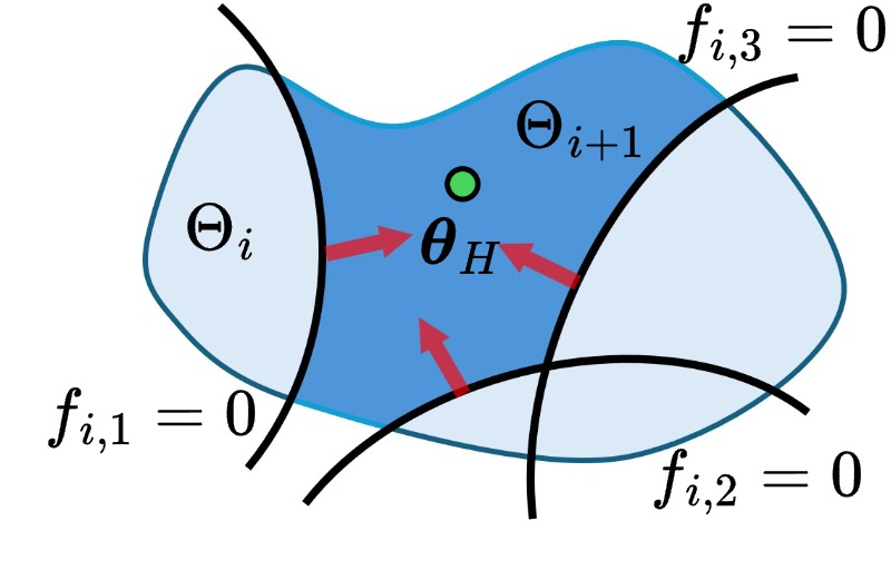
Figure 1: Illustration of one update from $\Theta_{i}$ to $\Theta_{i+1}$. Three constraints are induced from a human preference batch of size 3, with the simplified notation $f_{i,j}(\boldsymbol{\theta})=f(\boldsymbol{\theta},\boldsymbol{\xi}^{0}_{i,j},\boldsymbol{\xi}^{1}_{i,j},y_{i,j})$. Red arrows are the direction of the constraints, i.e., the $\boldsymbol{\theta}$ region satisfying $\{\boldsymbol{\theta}|f_{i,j}(\boldsymbol{\theta})\geq 0\}$. New $\Theta_{i+1}$ is the regions in $\Theta_{i}$ satisfying all constraints.

As shown in Fig. 1, the intuitive idea of the HSBC algorithm is to maintain and update a hypothesis space $\Theta_{i}$, starting from an initial set $\Theta_{0}$, based on batches of human preferences. Each batch of human preferences (Step 2) is actively queried. The human preference batch is turned into a batch cut (Step 3), removing portion of the current hypothesis space, leading to the next hypothesis space.

From (7) in (Step 3), it follows $\Theta_{0}\supseteq\Theta_{1}\supseteq\Theta_{2}\supseteq\dots$. This means that the hypothesis space is not increasing. More importantly, we have the following assertion, saying the human reward is always contained in the current hypothesis if all human preferences are true in a sense of (2).

Lemma 4.1.

If all human preferences are true, i.e., $y_{i,j}=y^{\text{true}}_{i,j},\ \forall i,j$ and $\boldsymbol{\theta}_{H}\in\Theta_{0}$, then following HSBC Algorithm, one has $\boldsymbol{\theta}_{H}\in\Theta_{i}$ for all $i=1,2,...,I$.

4.2 Voting Function for Human Preference Batch

In the HSBC algorithm, directly handling batch cut $\mathcal{C}_{i}$ and hypothesis space $\Theta_{i}$ can be computationally difficult, especially for high-dimensional parameter space e.g., neural networks. Thus, we will introduce a novel “voting function” to represent both.

Specifically, we define a voting function for a batch of human preferences $\mathcal{B}_{i}=\{{(\boldsymbol{\xi}^{0}_{i,j},\boldsymbol{\xi}^{1}_{i,j},y_{i,j})}\}^{N}_{j=1}$ as follows

$$V_{i}(\boldsymbol{\theta})=\sum\nolimits_{j=1}^{N}\mathrm{\mathbf{H}}(f(\boldsymbol{\theta},\boldsymbol{\xi}^{0}_{i,j},\boldsymbol{\xi}^{1}_{i,j},y_{i,j})),$$ (8)

where $H$ is the Heaviside step function defined as $\mathrm{\mathbf{H}}(x)=1$ if $x\geq 0$ and $\mathrm{\mathbf{H}}(x)=1$ otherwise. Intuitively, any point $\boldsymbol{\theta}\in\Theta$ in the hypothesis space will get a ”+1” vote if it satisfies $f(\boldsymbol{\theta},\boldsymbol{\xi}^{0}_{i,j},\boldsymbol{\xi}^{1}_{i,j},y_{i,j})\geq 0$ and “0” vote otherwise. Therefore, $V_{i}(\boldsymbol{\theta})$ represents the total votes of any point in the hypothesis space after the $i$th batch of human preferences.

Thus, $\boldsymbol{\theta}\in\mathcal{C}_{i}$ in (6) if and only if $V_{i}(\boldsymbol{\theta})=N$ because $\boldsymbol{\theta}$s need to satisfy all $N$ constraints $f(\boldsymbol{\theta},\boldsymbol{\xi}^{0}_{i,j},\boldsymbol{\xi}^{1}_{i,j},y_{i,j})\geq 0$ for $j=1,2,...,N$. As the number of votes in (8) only takes integers, the batch cut $\mathcal{C}_{i}$ can be equivalently written as:

$$\mathcal{C}_{i}=\{\boldsymbol{\theta}|V_{i}(\boldsymbol{\theta})\geq N-0.5\}.$$ (9)

Furthermore, the indicator of batch cut $\mathcal{C}_{i}$ can be written as:

$$\mathbbm{1}_{\mathcal{C}_{i}}(\boldsymbol{\theta})=\mathrm{\mathbf{H}}(V_{i}(\boldsymbol{\theta})-N+0.5).$$ (10)

Following (7) in the HSBC, since $\Theta_{i}=\Theta_{0}\cap\bigcap_{k=0}^{i-1}\mathcal{C}_{k}$, we can define the indicator function of the hypothesis space at $i$-th iteration:

$$\mathbbm{1}_{\Theta_{i}}(\boldsymbol{\theta})=\mathbbm{1}_{\Theta_{0}}(\boldsymbol{\theta})\prod\nolimits_{k=0}^{i-1}\mathbbm{1}_{\mathcal{C}_{k}}(\boldsymbol{\theta}),\quad i\geq 1$$ (11)

with $\mathbbm{1}_{\Theta_{0}}(\boldsymbol{\theta})$ be the indicator function of initial hypothesis space $\Theta_{0}$. With the indicator representation of $\Theta_{i}$ in (11), later we will show that $\boldsymbol{\theta}$ can be sampled from $\Theta_{i}$ as stated in (Step 1) in the HSBC algorithm.

4.3 Disagreement-Based Query and its Complexity

In the HSBC algorithm, not all batch cuts have similar effectiveness, i.e., some batch cut $\mathcal{C}_{i}$ can be redundant without removing any volume of hypothesis space, leading to an unnecessarily human query. To achieve effective cutting, each trajectory pair $(\boldsymbol{\xi}^{0}_{i,j},\boldsymbol{\xi}^{1}_{i,j},y_{i,j})$ should attain certain disagreement on the current hypothesis space $\Theta_{i}$, before sent to the human for preference query.

Specifically, in collecting human preference batch $\mathcal{B}_{i}$, we only query human preferences using trajectory pairs $(\boldsymbol{\xi}^{0}_{i,j},\boldsymbol{\xi}^{1}_{i,j},y_{i,j})$ that satisfy

$$\exists\,\,\boldsymbol{\theta}_{1},\boldsymbol{\theta}_{2}\in\Theta_{i},f(\boldsymbol{\theta}_{1},\boldsymbol{\xi}^{0}_{i,j},\boldsymbol{\xi}^{1}_{i,j},y_{i,j})\geq 0\\ \text{and}\ f(\boldsymbol{\theta}_{2},\boldsymbol{\xi}^{0}_{i,j},\boldsymbol{\xi}^{1}_{i,j},y_{i,j})\leq 0,\ \forall y_{i,j}$$ (12)

Intuitively, the disagreement-based query can ensure at least some portion of the hypothesis space is removed by the constraint $f(\boldsymbol{\theta},\boldsymbol{\xi}^{0}_{i,j},\boldsymbol{\xi}^{1}_{i,j},y_{i,j})\geq 0$ induced by $(\boldsymbol{\xi}^{0}_{i,j},\boldsymbol{\xi}^{1}_{i,j},y_{i,j})$, no matter what preference label $y_{i,j}$ human will provide. A geometric illustration is shown in Fig. LABEL:fig.cut_disagree, with the simplified notation $f_{i,j}(\boldsymbol{\theta})=f(\boldsymbol{\theta},\boldsymbol{\xi}^{0}_{i,j},\boldsymbol{\xi}^{1}_{i,j},y_{i,j})$. The above disagreement-based query strategies is also related to prior work (Christiano et al., 2017; Lee et al., 2021b).

With the disagreement-based preference query in each batch, the following assertion provides an upper bound on the total human query complexity of the HSBC algorithm given all true human preferences.

Theorem 4.2.

In the HSBC algorithm, suppose all true human preferences. Let $P(\boldsymbol{\xi}^{0},\boldsymbol{\xi}^{1},y^{\text{true}})$ be an unknown distribution of true human preferences. Define $\mathrm{err}(r_{\boldsymbol{\theta}})=P(f(\boldsymbol{\theta},\boldsymbol{\xi}^{0},\boldsymbol{\xi}^{1},y^{\text{true}})<0)$, which is the probability that $r_{\boldsymbol{\theta}}$ makes different predictions than human. For any $\epsilon,\delta$, the probability

$$P(\mathrm{err}(r_{\boldsymbol{\theta}})\leq\epsilon)\geq 1-\delta$$ (13)

holds with human query complexity:

$$K=NI\leq O(\zeta(d\log\zeta+\log\big{(}\log\frac{1}{\epsilon}/\delta\big{)})\log\frac{1}{\epsilon})$$ (14)

where $N$ and $I$ are the batch size and the iteration number,$\zeta$ is the disagreement coefficient related to the learning problem defined in Appendix E.2.3, and $d$ is the VC-dimension (Vapnik, 1998) of the reward model defined in Appendix E.1.

The above theorem shows that the proposed HSBC algorithm can achieve Probably Approximately Correct (PAC) learning of the human reward. The learned reward function $r_{\boldsymbol{\theta}}$ can make preference prediction with arbitrarily low error rate $\epsilon$ under arbitrary high probability $1-\delta$, under the human preference data complexity in (14).

5 Robust Alignment

In this section, we extend the HSBC algorithm to handle false human preference data. We will establish a provably robust learning process, such that the agent can still learn $\boldsymbol{\theta}_{H}$ regardless of the false human preference.

First, for a false human preference $(\boldsymbol{\xi}^{0},\boldsymbol{\xi}^{1},y^{\text{false}})$, it is easy to verify that (3) will lead to

$$\boldsymbol{\theta}_{H}\notin\{\boldsymbol{\theta}\in\Theta|f(\boldsymbol{\theta},\boldsymbol{\xi}^{0},\boldsymbol{\xi}^{1},y^{\text{false}})\geq 0\}$$ (15)

This means that a false human preference will also result in a constraint that $\boldsymbol{\theta}_{H}$ does not satisfy.

In the HSBC algorithm, suppose a batch $\mathcal{B}_{m}$ of human preference includes both true human preference labels and unknown false ones, i.e., $y_{m,j}$ is $y_{m,j}^{\text{true}}$ or $y_{m,j}^{\text{false}}$. We have the following lemma stating the failure of the method.

Lemma 5.1.

Following the HSBC Algorithm, if there exists one false preference in $m$-th batch $\mathcal{B}_{m}$ of human preferences, then $\boldsymbol{\theta}_{H}\notin\mathcal{C}_{m}$ and for all $i>m$, $\boldsymbol{\theta}_{H}\notin\Theta_{i}$.

Geometrically, Lemma 5.1 shows that any false human preference in preference batch $\mathcal{B}_{m}$ will make the batch cut $\mathcal{C}_{m}$ mistakenly “cut out” $\boldsymbol{\theta}_{H}$, i.e., $\boldsymbol{\theta}_{H}\in\mathcal{C}_{m}$. In the following, we show that the HSBC Algorithm will become provably robust by a slight modification of (6) or (9).

5.1 Cutting with Conservativeness Level $\gamma$

Our idea is to adopt a worst-case, conservative cut to handle unknown false human preferences in the HSBC algorithm. Specifically, let conservativeness level $\gamma\in[0,1]$ denote the ratio of the maximum number of false human preferences in a batch of $N$ human preferences. In other words, with $\gamma$, we suppose a preference batch has at most $\lceil\gamma N\rceil$ ($\lceil\cdot\rceil$ is the round-up operator) false preference. $\gamma$ is a worst-case or conservative estimate of false preference ratio and is not necessarily equal to the real error rate, which is unknown.

With the above conservativeness level $\gamma$, one can change (6) or (9) into following

$$\mathcal{C}_{i}=\{\boldsymbol{\theta}|V_{i}(\boldsymbol{\theta})>\lfloor(1-\gamma)N\rfloor-0.5\}$$ (16)

where $\lfloor\cdot\rfloor$ is the round-down operator, and the indicator function of the batch cut $\mathcal{C}_{i}$ thus can be expressed

$$\mathbbm{1}_{\mathcal{C}_{i}}(\boldsymbol{\theta})=\mathrm{\mathbf{H}}(V_{i}(\boldsymbol{\theta})-\lfloor(1-\gamma)N\rfloor+0.5)$$ (17)

The following important lemma states that only by the above modification of $\mathcal{C}_{i}$ without any other changes, the proposed HSBC algorithm can still achieve the provable robustness against false human preference.

Lemma 5.2.

With the conservativeness level $\gamma$ and replacing (6) with $\mathcal{C}_{i}$ in (16), the proposed HSBC Algorithm will have $\boldsymbol{\theta}_{H}\in\mathcal{C}_{i}$ and $\boldsymbol{\theta}_{H}\in\Theta_{i}$, i=1,2,3…I, regardless of false human preference.

The lemma means that by simply replacing expression (6) or (9) with $\eqref{equ.C_i_robust}$ while keeping other settings unchanged, the hypothesis cutting learning be performed in presence of the human false label. Actually, (9) is a special case of $\eqref{equ.C_i_robust}$ since when $\gamma=0$, $\lfloor(1-\gamma)N\rfloor=\lfloor N\rfloor=N$. A geometric interpretation of Lemma 5.2 is given below.

5.2 Geometric Interpretation

Fig. LABEL:fig.cuts shows a 2D geometric interpretation of the robust hypothesis cutting from $\Theta_{i}$ to $\Theta_{i+1}$ in the presence of false human preferences for batch $\mathcal{B}_{i}$. Suppose batch size $N=3$ and the third human preference $(\boldsymbol{\xi}^{0}_{i,3},\boldsymbol{\xi}^{1}_{i,3},y_{i,3}^{\text{false}})$ is false, while other two are true. Thus, we set $\gamma=1/3$ in (17).

As shown in Fig. LABEL:fig.cuts, since $(\boldsymbol{\xi}^{0}_{i,3},\boldsymbol{\xi}^{1}_{i,3},y_{i,3}^{\text{false}})$ is a false human preference, it will induce a constraint $f_{i,3}(\boldsymbol{\theta}):=f(\boldsymbol{\theta},\boldsymbol{\xi}^{0}_{i,3},\boldsymbol{\xi}^{1}_{i,3},y_{i,3}^{\text{false}})\geq 0$ which $\boldsymbol{\theta}_{H}$ does not satisfy. As a result, simply taking the intersection of all constraints $\{\boldsymbol{\theta}|f_{i,j}(\boldsymbol{\theta})\geq 0,j=1,2,3\}$ will rule out $\boldsymbol{\theta}_{H}$ by mistake. However, in this case, one can still perform a correct hypothesis space cutting (containing $\boldsymbol{\theta}_{H}$) using (17). Replacing $N=3$ and $\gamma=1/3$ in (17), the indicator function for the batched cut is $\mathbbm{1}_{\mathcal{C}_{i}}(\boldsymbol{\theta})=\mathrm{\mathbf{H}}(V_{i}(\boldsymbol{\theta})-1.5)$. This means by keeping the region in $\Theta_{i}$ with voting value $V_{i}(\boldsymbol{\theta})$ to be 2 or 3, $\boldsymbol{\theta}_{H}\in\Theta_{i+1}$.

6 Detailed Implementation

By viewing all true human preferences as a special case of robust cutting with conservativeness level $\gamma=0$, we present the implementation of the HSBC algorithm in Algorithm 1. The details are presented below.

Algorithm 1 Implementation for HSBC Algorithm

  Input: Batch size $N$, ensemble size $M$, conservativeness level $\gamma$, disagreement threshold $\eta$, segment count per trajectory $Z$.

  for $i=0$ to $I$ do   Sample an assemble $\mathcal{E}_{i}$ from current hypothesis space (if $i=0$, randomly initialize $\mathcal{E}_{0}$) with the method in Section 6.1. Filter and Densify $\mathcal{E}_{i}$ with the method in Section 6.2;   //Hypothesis Sampling   Based on $\mathcal{E}_{i}$, generate trajectory using sampling-based MPC (Section 6.3). Select trajectory pairs based on disagreement score, and acquire a preference batch $\mathcal{B}_{i}$ (Section 6.3);   //Disagreement-based human query   Update the sampling objective function with (20) and (21) using the new batch $\mathcal{B}_{i}$;   //Hypothesis space Cutting

  end for

  return $\mathcal{E}_{I}$

6.1 Hypothesis Space Sampling

The step of hypothesis space sampling is to sample an ensemble of $M$ parameters, $\mathcal{E}_{i}=\{\boldsymbol{\theta}^{k}_{i}\}_{k=1}^{M}$, from the current hypothesis space $\Theta_{i}$. We let the initial hypothesis space ${\Theta}_{0}=\mathbb{R}^{r}$, that is,

$$\mathbbm{1}_{\Theta_{0}}=1$$ (18)

which guarantees possible $\boldsymbol{\theta}_{H}$ is contained in $\Theta_{0}$. In our implementation, we use neural networks as our reward functions, thus $\mathcal{E}_{0}$ is randomly initialized common neural-network initialization distributions.

For $i>0$, sampling $\mathcal{E}_{i}$ can be reformulated as an optimization with the indicator function (11), i.e.,

$$\mathcal{E}_{i}\subseteq\arg\max_{\boldsymbol{\theta}}\mathbbm{1}_{\Theta_{i}}(\boldsymbol{\theta})=\arg\max_{\boldsymbol{\theta}}\prod\nolimits_{k=0}^{i-1}\mathbbm{1}_{\mathcal{C}_{k}}(\boldsymbol{\theta})$$ (19)

To use a gradient-based optimizer, (19) needs to be differentiable. Recall in (17) the only non-differentiable operation is $\mathrm{\mathbf{H}}$. Thus, we use the smooth sigmoid function $\mathrm{\mathbf{sig}}_{\rho}(\cdot)$ with temperature $\rho$ to approximate $\mathrm{\mathbf{H}}$. From (17), $\mathbbm{1}_{\mathcal{C}_{i}}$ will be replaced by the smooth approximation:

$$\hat{\mathbbm{1}}_{\mathcal{C}_{i}}(\boldsymbol{\theta})\approx\texttt{{sig}}_{\beta}\bigg{(}\sum_{j=1}^{N}\mathrm{\mathbf{sig}}_{\alpha}(f_{i,j}(\boldsymbol{\theta})){-}\nu(1{-}\gamma)N\bigg{)}$$ (20)

where $\alpha,\beta,\nu$ are the tunable learning parameters. Therefore, sampling $\mathcal{E}_{i}$ can be performed through

$$\mathcal{E}_{i}\subseteq\arg\max_{\boldsymbol{\theta}}\prod\nolimits_{k=0}^{i-1}\hat{\mathbbm{1}}_{\mathcal{C}_{k}}(\boldsymbol{\theta})$$ (21)

To get diverse $\boldsymbol{\theta}$ samples in $\mathcal{E}_{i}$, we optimize (21) in parallel with diverse initial guesses. For $i>0$, the optimization is warm-started using the previous $\mathcal{E}_{i-1}$ as initial values.

6.2 Sample Filtering and Densification

As ${\mathcal{E}_{i}}$ are solutions to a smoothed optimization (21), there is no guarantee that the samples are all in $\Theta_{i}$. Thus, we use the original indicator function $\mathbbm{1}_{\Theta_{i}}(\boldsymbol{\theta})$ to filter the collected samples: remove $\boldsymbol{\theta}$s that are not satisfying $\mathbbm{1}_{\Theta_{i}}(\boldsymbol{\theta})$. Since ${\mathcal{E}_{i}}$ after filtering may not have $M$ samples, we propose a densification step to duplicate some $\boldsymbol{\theta}$s (with also adding some noise) in ${\mathcal{E}_{i}}$ to maintain the same sample size $M$.

6.3 Reward Ensemble Trajectory Generation

With the ensemble $\mathcal{E}_{i}$ sampled from $\Theta_{i}$, the reward used for planning and control is defined by taking the mean value predicted of the reward ensemble, i.e.

$$r_{\mathcal{E}_{i}}(\boldsymbol{s},\boldsymbol{a})=\mathbb{E}_{\boldsymbol{\theta}\in\mathcal{E}_{i}}r_{\boldsymbol{\theta}}(\boldsymbol{s},\boldsymbol{a}).$$ (22)

In our implementation, we use sampling-based model predictive control (MPC) in the MJX simulator (Todorov et al., 2012) for trajectory generation. Half of the action plans generated from the MPC are perturbed with a decaying noise for exploration in the initial stage of learning. It is possible to using reinforcement learning for trajectory generation.

6.4 Disagreement Scoring and Query

In our algorithm, the generated trajectories are stored in a buffer. When a new trajectory is generated, we segment the new or each of the old trajectories (in the buffer) into $Z$ segments and randomly picking segment pairs $(\boldsymbol{\xi}^{0},\boldsymbol{\xi}^{1})$ for disagreement test. Here, $\boldsymbol{\xi}^{0}$ is from the new trajectory and $\boldsymbol{\xi}^{1}$ from the buffered trajectory.

For any segment pair $(\boldsymbol{\xi}^{0},\boldsymbol{\xi}^{1})$, we measure their disagreement on the current hypothesis space using the reward ensemble $\mathcal{E}_{i}$. We define the following disagreement score:

$$\texttt{{DIS}}_{\mathcal{E}_{i}}(\boldsymbol{\xi}^{0},\boldsymbol{\xi}^{1})={4n_{\mathcal{E}_{i}}^{+}n_{\mathcal{E}_{i}}^{-}}/{N^{2}}$$ (23)

where $n_{\mathcal{E}_{i}}^{+}$ is the number of $\boldsymbol{\theta}$s in $\mathcal{E}_{i}$ such that $J_{\boldsymbol{\theta}}(\boldsymbol{\xi}^{0})>J_{\boldsymbol{\theta}}(\boldsymbol{\xi}^{1})$ and $n_{\mathcal{E}_{i}}^{-}=N-n_{\mathcal{E}_{i}}^{+}$. When there is no disagreement in $\mathcal{E}_{i}$, i.e., $\boldsymbol{\theta}\in\mathcal{E}_{i}$ makes consensus judgment on $(\boldsymbol{\xi}^{0},\boldsymbol{\xi}^{1})$, $\texttt{{DIS}}_{\mathcal{E}_{i}}(\boldsymbol{\xi}^{0},\boldsymbol{\xi}^{1})=0$. When the disagreement is evenly split in , the score yields 1. In our implementation, a disagreement threshold $\eta\in(0,1)$ is defined to select valid disagreement pairs for human queries. A segment pair $(\boldsymbol{\xi}^{0},\boldsymbol{\xi}^{1})$ is rejected if $\texttt{{DIS}}_{\mathcal{E}_{i}}(\boldsymbol{\xi}^{0},\boldsymbol{\xi}^{1})\leq\eta$; otherwise, the human is queried for a preference label $y$ for $(\boldsymbol{\xi}^{0},\boldsymbol{\xi}^{1})$. Trajectory planning and the disagreement-based query are performed iteratively until $\mathcal{B}_{i}$ contains $N$ pairs.

7 Experiments

We test our method on 6 different tasks, as shown in Fig. LABEL:fig.tasks:

Cartpole
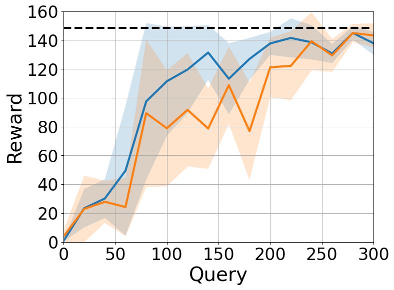
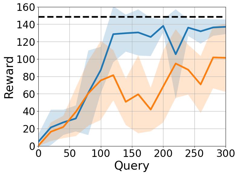
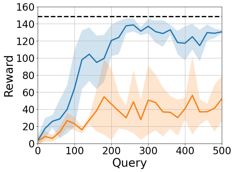
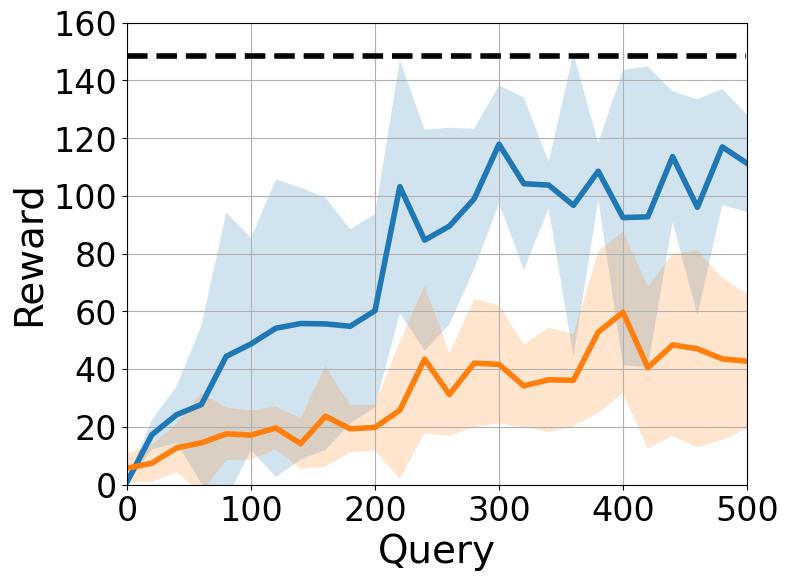
Walker
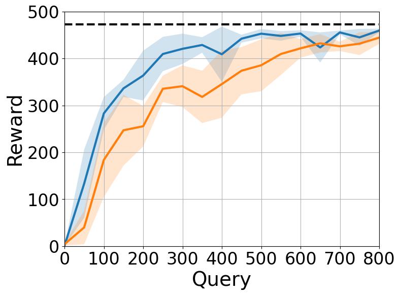
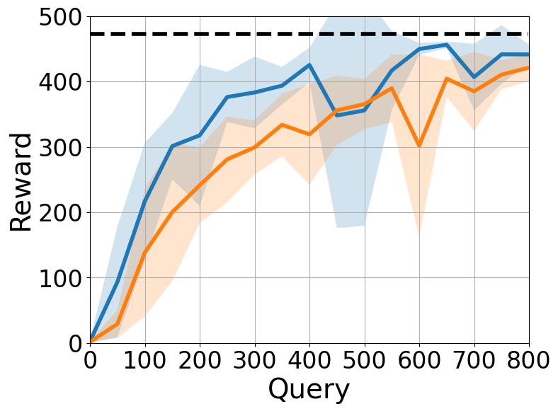
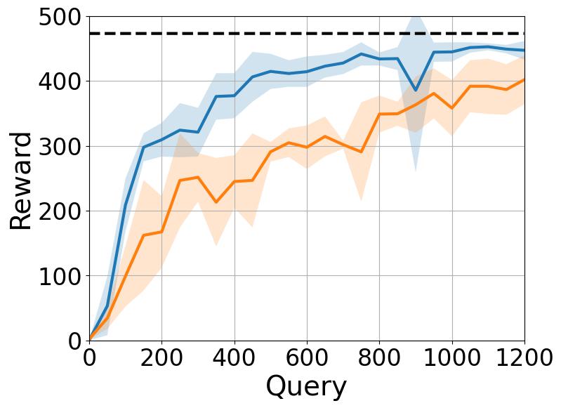
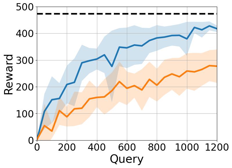
Humanoid

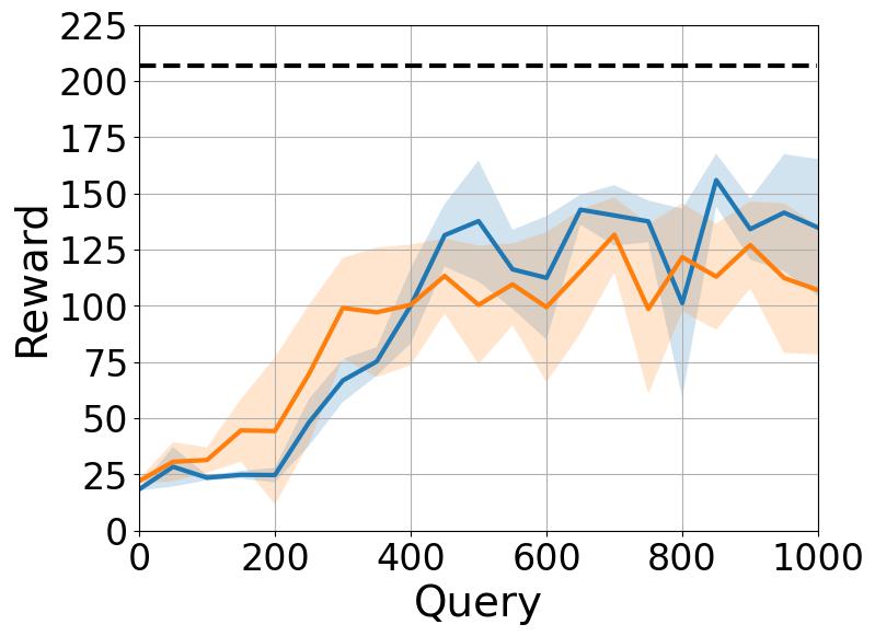
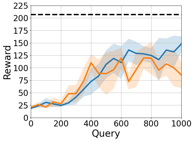
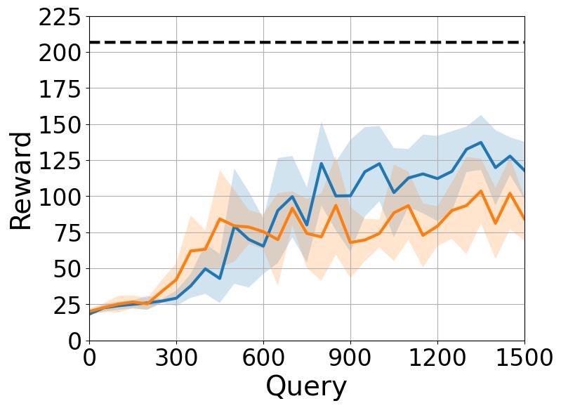
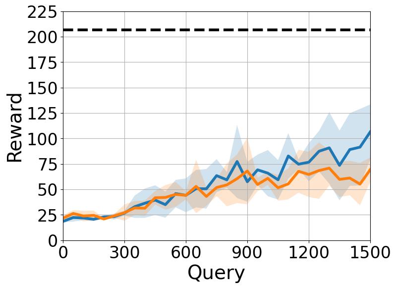
(a) False Rate $=0$       (b) False Rate $=10\%$     (c) False Rate $=20\%$     (d) False Rate $=30\%$

Figure 9: Learning curves of the dm-control tasks under different rates of false human preferences in different columns: (a) False Rate $=0$; (b) False Rate $=10\%$; (c) False Rate $=20\%$; (d) False Rate $=30\%$. The conservativeness level in HSBC algorithms is the same as the actual human false rate. All results are reported over 5 runs. The results show that our method significantly outperforms the baseline when the false rate is high, and has a comparable performance when the false rate is 0 (no false human preference).

DexMan-Cube
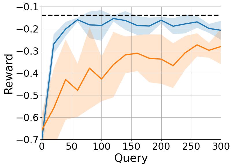
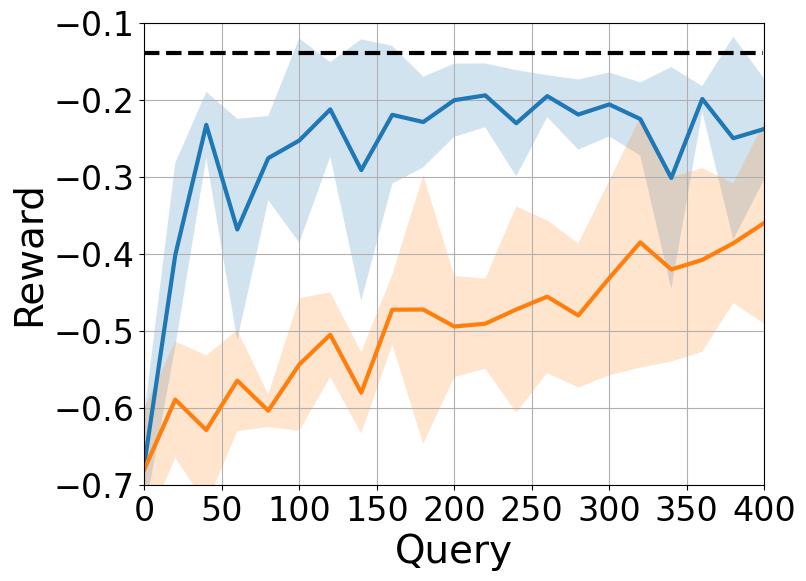
DexMan-Bunny
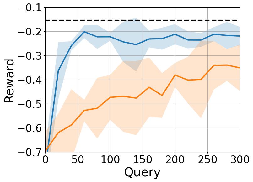
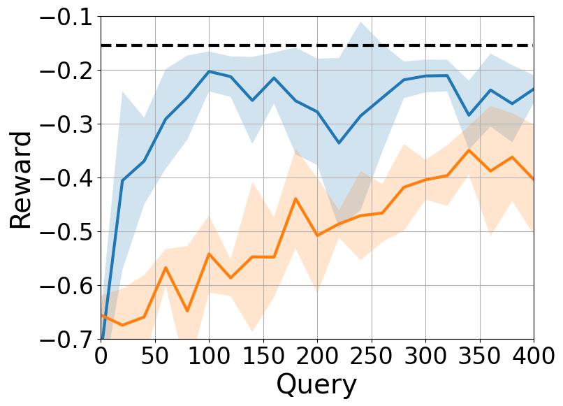
Go2-Standup

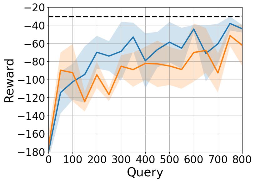
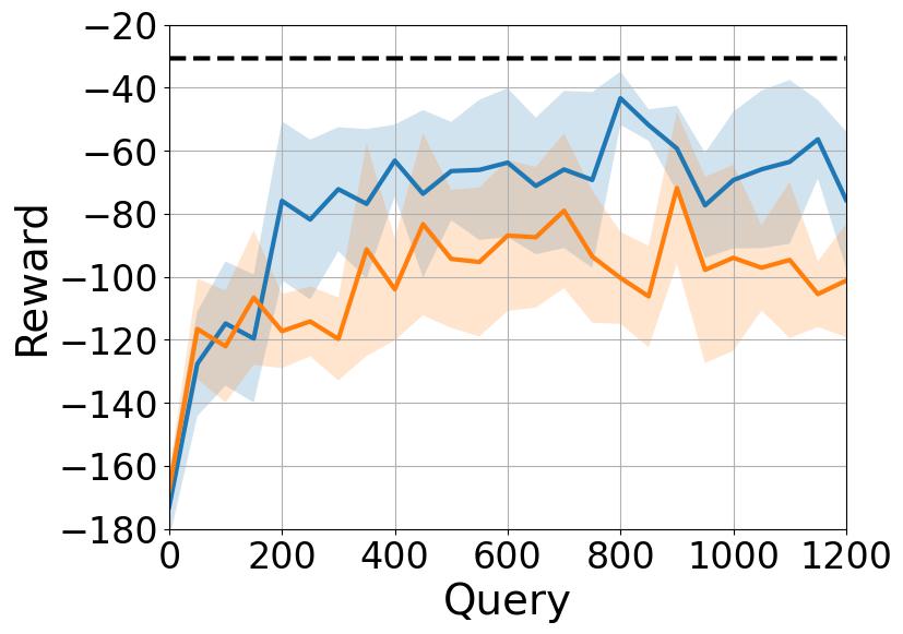
(a) False Rate $=0$       (b) False Rate $=20\%$

Figure 10: Learning curves for dexterous manipulation and locomotion tasks under different rates of false human preferences: (a) False Rate $=0$; (b) False Rate $=10\%$. The results are over 5 runs.

3 dm-control tasks: including Cartpole-Swingup, Walker-Walk, Humanoid-Standup.

2 in-hand dexterous manipulation tasks: An Allegro hand in-hand reorientate a cube and bunny object to any given target. The two objects demands different reward designs due to the geometry-dependent policy. We use DexMan-Cube and DexMan-Bunny to denote two tasks.

Quadruped robot stand-up task: A Go2 quadruped robot learns a reward to stand up with two back feet and raise the two front feet. We use Go2-Standup to denote the task.

More setting details are in Appendix B.3. Similar to MJPC (Howell et al., 2022) but to better support GPU-accelerated sampling-based MPC, we re-implemented all environments in MJX (Todorov et al., 2012) with MPPI (Williams et al., 2015) as MPC policy.

Table 1: Results on dm-control Tasks over 5 runs

Tasks		False Rate 0 %		False Rate 10%		False Rate 20%		False Rate 30%
	Oracle	Baseline	Ours	Baseline	Ours	Baseline	Ours	Baseline	Ours
Cartpole-Swingup	148.6	143.3 $\pm$8.3	137.8 $\pm$7.9	101.4 $\pm$39.2	137.0 $\pm$8.5	52.3 $\pm$26.8	130.7 $\pm$2.0	42.8 $\pm$23.3	111.3 $\pm$16.8
Walker-Walk	472.9	444.4 $\pm$13.4	459.4 $\pm$3.9	421.2 $\pm$20.6	441.4 $\pm$15.0	401.8 $\pm$37.6	447.1 $\pm$14.4	277.0 $\pm$62.3	417.2 $\pm$12.3
Humanoid-Standup	210.1	107.0 $\pm$28.6	134.7 $\pm$30.5	85.6 $\pm$25.9	148.0 $\pm$14.9	84.2 $\pm$15.2	117.9 $\pm$19.9	69.3 $\pm$12.0	106.5 $\pm$27.0

Table 2: Results on Dexterous Manipulation & Locomotion Tasks

Tasks		False Rate 0%		False Rate 20%
	Oracle	Baseline	Ours	Baseline	Ours
DexMan-Cube	-.14	-.28 $\pm$.08	-.20 $\pm$.04	-.36 $\pm$.13	-.24 $\pm$.06
DexMan-Bunny	-.16	-.35 $\pm$.09	-.22 $\pm$.04	-.40 $\pm$.10	-.24 $\pm$.03
Go2-Standup	-31	-62 $\pm$23	-44 $\pm$4	-101 $\pm$18	-76 $\pm$22

Simulated (false) human preference: Similar to (Lee et al., 2021b; Cheng et al., 2024), a “simulated human” is implemented as a computer program to provide preference for the reward learning. The simulated human uses the ground-truth reward $r_{\boldsymbol{\theta}_{H}}$ (see the ground truth reward of each task in Appendix B) to rank trajectory pairs. To simulate different rates of false human preferences, in each batch, a random selection of human preference labels is flipped.

Baseline Throughout the experiment, we compare our method against a baseline implemented using the reward learning approach from PEBBLE (details in Appendix A).

HSBC Algorithm settings: In all tasks, reward functions are MLP models. In our algorithm, unless specially mentioned, batch size $N=10$, ensemble size $M=16$, and disagreement threshold $\eta=0.75$. In dm-control tasks and Go2-Standup, trajectory pairs of the first few batches are generated by random policy for better exploration. Refer to Appendix C for other settings.

7.1 Results

For each task, we test our method and the baseline each for 5 independent runs with different random seeds. During the learning progress, the reward ensemble $\mathcal{E}_{i}$ at the checkpoint iteration $i$ is saved for evaluation. The evaluation involves using the saved reward ensemble $\mathcal{E}_{i}$ to generate a new trajectory, for which the performance is calculated using the ground-truth reward. Each evaluation is performed in 5 runs with different random seeds. Evaluation performance at different learning checkpoints will yield the learning curve. We show the learning curve in Fig. 9 for dm-control tasks, Fig. 10 for DexMan and Go2-Standup tasks. The mean and standard deviation across different runs are reported. To better show the human query complexity, we set the x-axis as the number of queries, and the y-axis is the performance of $\mathcal{E}_{i}$ control evaluated by ground-truth reward. Quantitatively, Table 1 and Table 2 show the evaluation reward results of the dm-control tasks and DexMan/Go2-Standup tasks.

From both Fig. 9 and Table 1, we observe a comparable performance of our proposed method and the baseline for zero false human preferences. Both methods successfully learn reward functions to complete different tasks. As the rate of false preference increases, from $10\%$ to $30\%$, we observe a significant performance drop of the baseline method. In contrast, the drop of the proposed method over a high rate of false human preference is not significant. These results demonstrate the robustness of the proposed method for reward learning against a high rate of false human preferences.

7.2 Ablation Study

Conservativeness level $\gamma$

Given a fixed rate of false human preference, We evaluate how different settings of conservativeness levels $\gamma=0,10\%,20\%,30\%$ affect the performance of the proposed method. Here, the actual human preferences have a fixed false rate of $20\%$. The ablation is tested for the Walker task, and the results over 5 runs are reported in Fig. LABEL:fig.ablation_gamma.

The results indicate that when $\gamma=0$ (i.e., the algorithm aggressively cuts the hypothesis space without conservatism), the learning performance drops significantly. Conversely, when the conservativeness level $\gamma=30\%$ exceeds the actual false rate ($20\%$) but remains within a reasonable range, it has little impact on learning performance. However, we postulate that, in general, a higher $\gamma$ increases query complexity, as less of the hypothesis space is cut per iteration.

Disagreement threshold $\eta$

We evaluate the performance of our algorithm under different disagreement thresholds $\eta$ given all true human preferences. The test is in Walker’s task. We set $\eta$ to 0, 0.5, 0.75 and show corresponding learning curves in Fig. LABEL:fig.ablation_eta. The results show that disagreement-based query can accelerate the learning convergence.

Batch size $N$

In Fig. LABEL:fig.ablation_M, we show the reward learning performance for the Walker task with different choices of preference batch sizes, $N=5,10,15,20$, under a fixed rate $20\%$ of false human preference. The results indicate a similar performance, suggesting that the learning performance is not sensitive to the setting of preference batch sizes.

8 Conclusion

In this paper, we propose the Hypothesis Space Batch Cutting (HSBC) method for robust reward alignment from human preference. Our method actively selects batches of preference data based on disagreement and uses them to constrain the reward function. Constraints in one batch are then grouped with a voting function, forming cuts to update the hypothesis space. To mitigate the false label in preference data, a conservative cutting method based on the voting function value is used to prevent overly aggressive cuts. HSBC is geometrically interpretable and provides a certifiable bound on query complexity. Tested across diverse control tasks, it matches baseline performance with clean data and outperforms it under high false preference rates.

Impact Statement

The HSBC method enhances interpretability and robustness in reward alignment by providing a geometric view of hypothesis updates and a certifiable bound on human query complexity. Its conservative cutting strategy ensures stable learning even in the presence of false preferences, making it resilient to noisy or adversarial data. These properties make HSBC particularly valuable in applications such as robotics, autonomous systems, and human-in-the-loop decision-making, where false data frequently present and reliable reward alignment with human intent is essential. By improving robustness while maintaining interpretability, HSBC offers a principled approach to preference-based learning in uncertain environments.

Appendix A Baseline Method for Comparison

We present the details of the baseline method used for comparison. It is inspired by the method of PEBBLE (Lee et al., 2021b) on training the reward model, while uses the same setting to plan the trajectories and collect the preferences. The only differences between the baseline and our method is the ensemble size and the objective function. An ensemble of 3 reward models is maintained. After $i$ batches of preference, the reward models are tuned to optimize the Bradley Terry loss function of all previous preferences:

$$\mathcal{L}=\sum_{k=0}^{i-1}\sum_{j=0}^{N-1}(1-y_{k,j})P_{\boldsymbol{\theta}}^{BT}(\boldsymbol{\xi}^{1}_{k,j}\succ\boldsymbol{\xi}^{0}_{k,j})+y_{k,j}P_{\boldsymbol{\theta}}^{BT}(\boldsymbol{\xi}^{1}_{k,j}\succ\boldsymbol{\xi}^{0}_{k,j})$$ (24)

where

$$P_{\boldsymbol{\theta}}^{BT}(\boldsymbol{\xi}^{0}\succ\boldsymbol{\xi}^{1})=\frac{\exp{\alpha_{base}J_{\boldsymbol{\theta}}(\boldsymbol{\xi}^{0})}}{\exp{\alpha_{base}J_{\boldsymbol{\theta}}(\boldsymbol{\xi}^{0})}+\exp{\alpha_{base}J_{\boldsymbol{\theta}}(\boldsymbol{\xi}^{1})}}$$ (25)

The parameter $\alpha_{base}$ is the temperature of the Bradley-Terry model. In the dexterous manipulation tasks, $\alpha_{base}=0.5$. In all other tasks, $\alpha_{base}=3$. In the experiments of cartpole swingup, $\alpha_{base}=10$. The preferences are selected with disagreement threshold $\eta=0.8$, which is similar to our approach.

Appendix B Detailed Description of the Tasks

B.1 DM-Control Tasks

We re-implemented three dm-control tasks in MJX to perform sampling-based MPC, similar to (Howell et al., 2022).

Cartpole

We directly use the environment xml file in dm-control, with the same state and action definition in original library. The goal is to swing up the pole to an upright position and balance the system in the middle of the trail. Use $\varphi,\dot{\varphi}$ to denote the angle and angular velocity of the pole, $x,\dot{x}$ to denote the horizontal position and velocity of the cart. The system is initialized with $x=0$ and $\varphi=\pi$, along with a normal noise with standard deviation 0.01 imposed on all joint positions and velocities. $\boldsymbol{s}=(x,\sin\varphi,\cos\varphi,\dot{x},\dot{\varphi})$ and $\boldsymbol{a}$ is a 1D control scalar signal for the horizontal force applied on the cart. We use a ground truth reward function:

$$r(\boldsymbol{s},\boldsymbol{a})=\mathrm{upright}(\boldsymbol{s})*\mathrm{middle}(\boldsymbol{s})*\mathrm{small\_ctrl}(\boldsymbol{a})*\mathrm{small\_vel}(\boldsymbol{s})$$ (26)

where $\mathrm{upright}(\boldsymbol{s})=(\cos\varphi+1)/2$, $\mathrm{middle}(\boldsymbol{s})=\exp(-x^{2})$, $\mathrm{small\_ctrl}(\boldsymbol{a})=(4+\exp(-4\boldsymbol{a}^{2}))/5$, $\mathrm{small\_vel}(\boldsymbol{s})=(1+\exp(-0.5\dot{x}^{2}))/2$.

Walker-Walk

We directly use the environment xml file in dm-control. The goal is to make the agent walk forward with a steady speed.The system is initialized at a standing position and a normal noise with standard deviation 0.01 is imposed on all joint positions and velocities. Use $z$ to denote the sum of $z-$coordinate of the torso and a bias $-1.2$, thus the value $z=0$ when the walker stands up-straight. $\varphi_{y}$ to denote the torso orientation in $xz-$plane, $q$ to denote all joints between links and $\dot{x}$ to denote the torso linear velocity on $x-$axis. $\boldsymbol{s}=(z,\varphi_{y},q,\dot{x},\dot{z},\dot{\varphi_{y}},\dot{q})$ and $\boldsymbol{a}\in[0,1]^{6}$ stands for torques applied on all joints. We use a ground truth reward function:

$$r(\boldsymbol{s},\boldsymbol{a})=\frac{3*\mathrm{standing}(\boldsymbol{s})+\mathrm{upright}(\boldsymbol{s})}{4}*\mathrm{move}(\boldsymbol{s})$$ (27)

where $\mathrm{standing}(\boldsymbol{s})=\mathrm{clip}(1-|z|,0,1)$, $\mathrm{upright}(\boldsymbol{s})=(\cos\varphi_{y}+1)/2$, $\mathrm{move}(\boldsymbol{s})=\mathrm{clip}(\dot{x},0,1)$.

Humanoid-Standup

We directly use the environment xml file in dm-control. The goal is to stand up from a lying position. The system is initialized at a lying position and a uniform noise between -0.01 and 0.01 is imposed on all joint positions and velocities. Use $z,quat$ to denote the $z-$coordinate and quaternion orientation of the humanoid torso. Use $v=[v_{x},v_{y},v_{z}],w=[w_{x},w_{y},w_{z}]$ to denote 3D linear and angular velocity of the torso. Use $q$ to denote all of the joints in humanoid agent. $\boldsymbol{s}=[z,quat,q,v,w,\dot{q}]$ and $\boldsymbol{a}\in[0,1]^{17}$ stands for torques applied on all joints. We use a ground truth reward function:

$$r(\boldsymbol{s},\boldsymbol{a})=\mathrm{standing}(\boldsymbol{a})*\mathrm{small\_vel}(\boldsymbol{s})$$ (28)

where $\mathrm{standing}(\boldsymbol{s})=\mathrm{clip}(z/1.2,0,1)$ and $\mathrm{small\_vel}(\boldsymbol{s})=\exp(-0.1*\sqrt{v_{x}^{2}+v_{y}^{2}}-0.3\left\lVert w\right\rVert)$.

B.2 In-hand Dexterous Manipulation

We mainly focus on Allegro robot in-hand re-orientation of two different objects, a cube and a bunny. An allegro hand and an object are simulated in the environment. The allegro hand is tilted with quaternion $[0.0,0.82,0.0,0.57]$. The objects has initial position of $[0.0,0.0,0.05]$ with quaternion $[0,0,0,1]$ In the beginning of every trajectory planning during training, a target orientation in the form of an axis-angle is randomly selected. The axis is uniformly randomly selected from $x,y,z$ axis and the angle is uniformly randomly selected from the set $\{\pm\frac{\pi}{4},\pm\frac{\pi}{2},\pm\frac{3\pi}{4},\pi\}$. This angle-axis rotation is then converted to target quaternion $q_{targ}$. The goal is to use the fingers of the robotic hand to rotate the object to the target orientation, as well as remain the object in the center of the hand. Use $q$ to denote the joint positions of the robot hand, $p$ to denote the object position, $\Delta quat$ to denote the quaternion different between current object pose and target pose ($\Delta quat=1-(q_{curr}^{T}q_{targ})^{2}$) and $ff_{tip},mf_{tip},rf_{tip},th_{tip}$ to denote the positions of four fingertips (forefinger, middle finger, ring finger and thumb). The object and fingertip positions are multiplied by 10 to balance the scale. $\boldsymbol{s}=[q,p,\Delta quat,ff_{tip},mf_{tip},rf_{tip},th_{tip}]$. $\boldsymbol{a}\in[0,1]^{12}$ is the delta-position command on all joints and is multiplied by 0.2 to generate actual control signals. The ground truth reward is designed to be:

$$r(\boldsymbol{s},\boldsymbol{a})=-\mathrm{cost\_quat}(\boldsymbol{s})-0.4\mathrm{cost\_pos}(\boldsymbol{s})-0.05\mathrm{cost\_contact}(\boldsymbol{s})$$ (29)

Where $\mathrm{cost\_quat}(\boldsymbol{s})=\Delta quat$, $\mathrm{cost\_pos}(\boldsymbol{s})=\left\lVert p-(0.0,0.0,0.01)*10\right\rVert^{2}$ and $\mathrm{cost\_contact}(\boldsymbol{s})=\left\lVert p-ff_{tip}\right\rVert^{2}+\left\lVert p-mf_{tip}\right\rVert^{2}+\left\lVert p-rf_{tip}\right\rVert^{2}+\left\lVert p-th_{tip}\right\rVert^{2}$.

In evaluation, 6 trajectories are planned by setting different target of $\pm\frac{\pi}{2}$ rotation on $x,y,z$ axis. The mean reward per trajectory per time step is calculated and recorded.

B.3 Go2-Standup

In this task, a go2 quadruped robot is simulated and the goal is to stand up on two back feet to keep the torso height on $0.6$, and raise two front feet to the height of $1.2$. The initial pose and the target pose is shown in Fig. LABEL:fig.Go2. The system is initialized at a standing position on four legs and a uniform noise between -0.01 and 0.01 is imposed on all joint positions and velocities. Use $z_{t},quat$ to denote the $z-$coordinate and quaternion orientation of the robot torso. Use $z_{ff},z_{rf}$ to denote $z-$coordinates of two front feet and two rear feet. To balance the scale, all features related to the $z$-coordinates are multiplied by 10. Use $v=[v_{x},v_{y},v_{z}],w=[w_{x},w_{y},w_{z}]$ to denote 3D linear and angular velocity of the torso. Use $q$ to denote all of the joint positions. $\boldsymbol{s}=[z_{t},quat,q,z_{ff},z_{rf},v,w,\dot{q}]$ and $\boldsymbol{a}\in[0,1]^{12}$ stands for the desired delta-position on all joints. We define the ground truth reward function as:

$$r(\boldsymbol{s},\boldsymbol{a})=-2.5\mathrm{height\_cost}(\boldsymbol{s})-0.5\mathrm{feet\_cost}(\boldsymbol{s})-10^{-6}\mathrm{ang\_vel\_cost}(\boldsymbol{s})-10^{-2}\mathrm{vel\_cost}(\boldsymbol{s})$$ (30)

where $\mathrm{height\_cost}(\boldsymbol{s})=(z-0.6)^{2}$, $\mathrm{feet\_cost}(\boldsymbol{s})=\left\lVert z_{ff}-1.2\right\rVert^{2}+\left\lVert z_{rf}\right\rVert^{2}$, $\mathrm{ang\_vel\_cost}(\boldsymbol{s})=\left\lVert w\right\rVert^{2}$ and $\mathrm{vel\_cost}(\boldsymbol{s})=\left\lVert v\right\rVert^{2}$.

Appendix C Model and Parameters in Experiment

Reward Neural Networks

For all tasks, we use an MLP with 3 hidden layers of 256 hidden units to parameterize reward functions. The activation function of the network is ReLU. In the dm-control tasks, the input is a concatenated vector of state $\boldsymbol{s}$ and action $\boldsymbol{a}$. In dexterous manipulation and quadruped locomotion tasks, the input is purely the state $\boldsymbol{s}$ to perform faster learning. The output scalar value of the reward is scaled to the interval $[-1,1]$ using the Tanh function. In particular, in the dexterous manipulation tasks, an intrinsic reward $-0.5\mathrm{cost\_contact}(\boldsymbol{s})$ is imposed to the network output, forming a predicted reward to encourage grasping the object and bootstrapping the learning.

Learning Settings

The parameters $\alpha,\beta,Z,I,T$, segment length $T_{seg}$ and evaluation trajectory length $T_{eval}$ slightly varies from the tasks, see Table 3. In the Table, the two number of batch number $K$ corresponds to the number with irrationality 0 and 20%. The Adam (Kingma, 2014) optimizer parameter is identical for all dm-control and Go2-Standup tasks, the learning rate is set to be 0.005 with a weight decay coefficient 0.001. In dexterous manipulation tasks, the learning rate is 0.002 with a weight decay coefficient 0.001.

Table 3: Learning Parameter in Different Tasks

Task	$\alpha$	$\beta$	$Z$	$I$	$T$	$T_{eval}$	$T_{seg}$
Cartpole-Swingup	10.0	3.0	2	50/80	100	200	50
Walker-Walk	5.0	3.0	2	80/120	150	500	50
Humanoid-Standup	5.0	3.0	3	100/150	200	300	50
DexMan-Cube	5.0	3.0	3	30/40	100	150	20
DexMan-Bunny	5.0	3.0	3	30/40	100	150	20
Go2-Standup	5.0	3.0	3	80/120	150	100	25

MPPI Parameter

The number of samples ($\mathrm{Num}$), planning horizon ($\mathrm{Hor}$), temperature ($\lambda$) and the standard deviation ($\mathrm{Std}$) of the normal sampling distribution determines the quality of trajectories planned by MPPI. These parameters varies from different tasks, see Table 4. In the table, two numbers on each entry denotes the different setting in training and evaluation stage.

Table 4: MPPI Parameter in Different Tasks

Task	$\mathrm{Num}$	$\mathrm{Hor}$	$\lambda$	$\mathrm{Std}$
Cartpole-Swingup	256/512	20/25	0.01/0.01	1.0/0.75
Walker-Walk	512/1024	25/30	0.01/0.01	1.0/0.75
Humanoid-Standup	1024/1024	25/25	0.01/0.01	1.2/0.75
DexMan-Cube	1024/1024	5/5	0.01/0.01	1.0/1.0
DexMan-Bunny	1024/1024	5/5	0.01/0.01	1.0/1.0
Go2-Standup	1024/1024	25/25	0.005/0.01	1.0/0.75

Appendix D Proof of the Lemmas

D.1 Proof of Lemma 4.1

Proof.

By the definition of $y^{\text{true}}$ in (2),

$$f(\boldsymbol{\theta},\boldsymbol{\xi}^{0}_{i,j},\boldsymbol{\xi}^{1}_{i,j},y^{\text{true}}_{i,j})\geq 0$$ (31)

combining the definition of $\mathcal{C}_{i}$ in (6), $\boldsymbol{\theta}_{H}\in\mathcal{C}_{i},\ \forall i$. Hypothesis space $\Theta_{i}=\Theta_{0}\cap\mathcal{C}_{0}\cap\cdots\cap\mathcal{C}_{i-1}$. Combining $\boldsymbol{\theta}_{H}\in\Theta_{0}$ and $\boldsymbol{\theta}_{H}\in\mathcal{C}_{i},\ \forall i$, $\boldsymbol{\theta}_{H}\in\Theta_{i},\ \forall i$. ∎

D.2 Proof of Lemma 5.1

Proof.

Without loss of generality, suppose $j$th preference in $m$th batch $(\xi^{(0)}_{m,j},\xi^{(1)}_{m,j},y^{\text{false}}_{m,j})$ has false label, Thus,

$$f_{m,j}(\boldsymbol{\theta}_{H})<0$$ (32)

Which means $\boldsymbol{\theta}_{H}\notin\mathcal{C}_{m}$. With definition of $\mathcal{C}_{m}$ and $\Theta_{i}$, for all $i>m$,

$$\Theta_{i}\subseteq\Theta_{m}\subseteq\mathcal{C}_{m}$$ (33)

that leads to $\boldsymbol{\theta}_{H}\notin\Theta_{i}$ for all $i>m$. ∎

D.3 Proof of Lemma 5.2

Proof.

With the definition of $\gamma$, there are at most $\lceil\gamma N\rceil$ incorrect labels and at least $\lfloor(1-\gamma)N\rfloor$ correct labels in one batch $\mathcal{B}_{i}$. For all $\boldsymbol{\theta}_{H}\in\Theta_{H}$, $f_{i,j}(\theta_{H})\geq 0$ holds for all tuples with correct labels $(\xi^{0}_{i,j},\xi^{1}_{i,j},y^{\text{true}}_{i,j})$. As a result, in the voting process of $V_{i}(\boldsymbol{\theta}_{H})$ shown in (8), there will be at least $\lfloor(1-\gamma)N\rfloor$ ”+1” votes and $V_{i}(\boldsymbol{\theta}_{H})\geq\lfloor(1-\gamma)N\rfloor$. With the modified definition of $\mathcal{C}_{i}$ in (16), $\boldsymbol{\theta}_{H}\in\mathcal{C}_{i}$ and we have $\boldsymbol{\theta}_{H}\in\Theta_{i}$ ∎

Appendix E Proof of the Theorem 4.2

The proof of the theorem follows the pipeline in Chapter 6 in (Settles, 2012). In order for the paper to be self-contained, we include the complete proof here.

E.1 Reward-Induced Classifier

The preference alignment can be viewed as a classification task. Use the new notation $x=(\boldsymbol{\xi}^{0},\boldsymbol{\xi}^{1})$ to denote a trajectory pair. This pair is fed to the classifier to predict a 0-1 label $y$ of which trajectory is better in human’s sense. For any parameterized reward model $r_{\boldsymbol{\theta}}$, a classifier $h_{\boldsymbol{\theta}}$ can be induced by defining:

$$h_{\theta}(x)=\begin{cases}0,J_{\boldsymbol{\theta}}(\boldsymbol{\xi}^{0})\geq J_{\boldsymbol{\theta}}(\boldsymbol{\xi}^{1})\\ 1,J_{\boldsymbol{\theta}}(\boldsymbol{\xi}^{0})<J_{\boldsymbol{\theta}}(\boldsymbol{\xi}^{1})\\ \end{cases}$$ (34)

Recall that function $g$ is used to calculate the average reward on any trajectory. All of the classifiers induced by $r_{\theta}$ parameterized by $\theta\in\Theta_{0}$ forms a concept class $\mathcal{H}=\{h_{\theta}|\theta\in\mathbb{R}^{r}\}$. We assume the VC dimension of $\mathcal{H}$ is a finite number $d$.

Specifically, there is a human classifier correspond to $r_{\boldsymbol{\theta}_{H}}$ which defines the label $y$ corresponds to $x$:

$$y=h_{H}(x)=\begin{cases}0,J_{\boldsymbol{\theta}_{H}}(\boldsymbol{\xi}^{0})\geq J_{\boldsymbol{\theta}_{H}}(\boldsymbol{\xi}^{1})\\ 1,J_{\boldsymbol{\theta}_{H}}(\boldsymbol{\xi}^{0})<J_{\boldsymbol{\theta}_{H}}(\boldsymbol{\xi}^{1})\\ \end{cases}$$ (35)

Using $P_{XY}$ to denote the data-label joint distribution and use $P_{X}$ to define the marginal distribution of $x$ for simplicity. There exists one aligned classifier $h^{*}\in\mathcal{H}$ such that:

$$\forall x,y\sim P_{XY},h^{*}(x)=y$$ (36)

Define the error rate of any $h\in\mathcal{H}$ as:

$$\mathrm{err}(h)=P_{X}(h(x)\neq h^{*}(x)),$$ (37)

it is equivalent to express the preference prediction error rate $\mathrm{err}(r_{\boldsymbol{\theta}})=P(f(\boldsymbol{\theta},\boldsymbol{\xi}^{0},\boldsymbol{\xi}^{1},y^{\text{true}})<0)$ in Theorem as $\mathrm{err}(r_{\boldsymbol{\theta}})=\mathrm{err}(h_{\boldsymbol{\theta}})$.

E.2 Definition of some Helper Functions, Sets and Coefficients

In this section we establish some definitions of helper functions, sets or coefficients, which are used in the main proof of Theorem 4.2.

E.2.1 Version Space

Similar to the definition of $\mathcal{H}$, the classifier set generated by every $\Theta_{i}$ can be notes as $\mathcal{V}_{i}=\{h_{\boldsymbol{\theta}}|{\boldsymbol{\theta}}\in\Theta_{i}\}$, which is typically called version space in the context of active learning. By the definition of $\Theta_{i}$, for all $h\in\mathcal{V}_{i}$, $h$ can make perfect classfication of all data $(x,y)$ formed by the trajectory pairs and labels in all previous batches $\mathcal{B}_{0},\dots\mathcal{B}_{i-1}$. Also, since $\Theta_{H}\subseteq\Theta_{i}$, $h^{*}\in\mathcal{V}_{i}$ for all the time. Because the hypothesis space for parameters is shrinking, i.e., $\Theta_{i}\supseteq\Theta_{i+1}$, the version space is also shrinking such that $\mathcal{V}_{i}\supseteq\mathcal{V}_{i+1}$.

E.2.2 Difference between Classifiers on $\Xi$ and Corresponding Balls

The data distribution provides straightforward measure between two classifiers $h_{1},h_{2}\in\mathcal{H}$, by directly examine the porpotion of data that they behaves differently. A difference $\Delta(h_{1},h_{2})$ can be defined as the probability of two classifiers behaves differently, under the data distribution $\Xi$:

$$\Delta(h_{1},h_{2})=P_{X}(h_{1}(x)\neq h_{2}(x))$$ (38)

With this different as a distance measure, an $\rho-$ball with radius $\rho$ and center $h_{c}$ can be defined as:

$$B(h_{c},\rho)=\{h\in\mathcal{H}|\Delta(h_{c},h)\leq\rho\}$$ (39)

E.2.3 Region of Disagreement and Disagreement Coefficient

For a given version space $\mathcal{V}$ and use $\mathcal{X}$ to denote the instance space of $x$, the region of disagreement is a subset of the instance space:

$$\mathrm{DIS}(\mathcal{V})=\{x\in\mathcal{X}|\exists h_{1},h_{2}\in\mathcal{V}:h_{1}(x)\neq h_{2}(x)\}$$ (40)

With the definition of the region of disagreement, a disagreement coefiicient was propose by (Hanneke, 2007) to characterize the difficulty of active learning, which is defined with the expression

$$\zeta=\sup_{\rho>0}\frac{P_{X}(\mathrm{DIS}(B(h^{*},\rho)))}{\rho}$$ (41)

The value $\zeta$ is determined by $\mathcal{H}$ and $\Xi$. The greater $\zeta$ is, the more the volume of the disagreement region of the $\rho-$ball around $h^{*}$ scales with $\rho$, which signified greater learning difficulty.

E.3 Passive PAC Sample Complexity Bound

Since the training set from the distribution $\Xi_{XY}$ is perfectly seperateble as in, using the famous probably approximately correct (PAC) bound for passive learning, with arbitary $\epsilon$ and $\delta$, $P(\mathrm{err}(h)\leq\epsilon)\geq 1-\delta$ can be achieved by perfectly fit training data with size $L_{PASS}$:

$$L_{PASS}\leq O(\frac{1}{\epsilon}(d\log(\frac{1}{\epsilon})+\log\frac{1}{\delta}))\simeq O(\frac{d}{\epsilon})$$ (42)

E.4 Formal Proof of Theorem 4.2

Proof.

For arbitary $\epsilon$ and $\delta$, define batch size $N$ to be:

$$N=\lceil c\zeta(d\log\zeta+\log\frac{1}{\delta^{\prime}})\rceil$$ (43)

with $c$ as a constant and a sepcialy chosen $\delta^{\prime}$ (the definition of which is shown later in the proof). With probability $1-\delta^{\prime}$ and for all $h\in\mathcal{V}_{i+1}$:

$$P_{X}(h(x)\neq h^{*}(x)|x\in\mathrm{DIS}(\mathcal{V}_{i}))\leq\frac{c^{\prime}}{N}(d\log\frac{N}{d}+\log\frac{1}{\delta^{\prime}})$$ (44)

This is because data batch $\mathcal{B}_{i}$ is selected by disagreement (12). By the definition of $\mathcal{V}_{i+1}$, all of the data $\mathcal{B}_{i}$ comes from the set $\mathrm{DIS}(\mathcal{V}_{i})$ and all of the classifiers in $\mathcal{V}_{i+1}$ perfectly fits this batch. By switching the PAC bound $L_{PASS}$ in Appendix E.3 with $M$ and solves for $\epsilon$ we get the RHS of the inequality.

With proper choice of $c,c^{\prime}$, $\log\frac{N}{d}\leq\log\zeta$ and the RHS of (44):

$$\frac{c^{\prime}}{N}(d\log\frac{N}{d}+\log\frac{1}{\delta^{\prime}})\leq\frac{c^{\prime}}{c\zeta}\leq\frac{1}{2\zeta}$$ (45)

As a result, for all $h\in\mathcal{V}_{i+1}$,

$$\mathrm{err}(h)= P_{X}(h(x)\neq h^{*}(x))$$ (46)

$$= P_{X}(h(x)\neq h^{*}(x)|x\in\mathrm{DIS}(\mathcal{V}_{i}))P_{X}(x\in\mathrm{DIS}(\mathcal{V}_{j}))+$$ (47)

$$P_{X}(h(x)\neq h^{*}(x)|x\notin\mathrm{DIS}(\mathcal{V}_{i}))P_{X}(x\notin\mathrm{DIS}(\mathcal{V}_{j}))$$ (48)

By the property $\mathcal{V}_{i+1}\subseteq\mathcal{V}_{i}$, $h\in\mathcal{V}_{i}$ and combining with $h^{*}\in\mathcal{V}_{i}$, $P_{X}(h(x)\neq h^{*}(x)|x\notin\mathrm{DIS}(\mathcal{V}_{i}))=0$ and

$$\mathrm{err}(h)\leq\frac{P_{X}(x\in\mathrm{DIS}(\mathcal{V}_{i}))}{2\zeta}=\frac{P_{X}(\mathrm{DIS}(\mathcal{V}_{i}))}{2\zeta}$$ (49)

This means $\mathcal{V}_{i+1}\subseteq B(h^{*},\frac{P_{X}(\mathrm{DIS}(\mathcal{V}_{i}))}{2\zeta})$, with the definition of the disagreement coefficient $\zeta$,

$$P_{X}(\mathrm{DIS}(\mathcal{V}_{i+1}))\leq P_{X}(\mathrm{DIS}(B(h^{*},\frac{P_{X}(\mathrm{DIS}(\mathcal{V}_{i}))}{2\zeta})))\leq\frac{P_{X}(\mathrm{DIS}(\mathcal{V}_{i}))}{2}$$ (50)

Thus, let $U_{0}=P_{X}(\mathrm{DIS}(\mathcal{V}_{0}))/2\zeta$, after $I=\log_{2}(U_{0}/\epsilon)$ batches of data and with $\delta^{\prime}=\delta/I$, for all $h\in\mathcal{V}_{I}$, The relationship

$$\mathrm{err}(h)\leq U_{0}2^{-I}=\epsilon$$ (51)

holds with a union bound probability $1-I\delta^{\prime}=1-\delta$. With the definition of $\mathcal{V}_{I}$, for all $\theta\in\Theta_{I}$, $\mathrm{err}(r_{\theta})=\mathrm{err}(h_{\theta}\in\mathcal{V}_{I})\leq\epsilon$. Thus, the total number of the quries to perform PAC alignment can be expressed as:

$$K=IN=O(\zeta(d\log\zeta+\log\frac{\log 1/\epsilon}{\delta})\log\frac{1}{\epsilon})$$ (52)

This is the bound shown in Theorem 4.2 and completes the proof. ∎

References

- Achiam et al. (2023) Achiam, J., Adler, S., Agarwal, S., Ahmad, L., Akkaya, I., Aleman, F. L., Almeida, D., Altenschmidt, J., Altman, S., Anadkat, S., et al. Gpt-4 technical report. arXiv preprint arXiv:2303.08774, 2023.
- Akrour et al. (2012) Akrour, R., Schoenauer, M., and Sebag, M. April: Active preference learning-based reinforcement learning. In Machine Learning and Knowledge Discovery in Databases: European Conference, ECML PKDD 2012, Bristol, UK, September 24-28, 2012. Proceedings, Part II 23, pp. 116–131. Springer, 2012.
- Akrour et al. (2014) Akrour, R., Schoenauer, M., Sebag, M., and Souplet, J.-C. Programming by feedback. In International Conference on Machine Learning, volume 32, pp. 1503–1511. JMLR. org, 2014.
- Amid et al. (2019) Amid, E., Warmuth, M. K., Anil, R., and Koren, T. Robust bi-tempered logistic loss based on bregman divergences. Advances in Neural Information Processing Systems, 32, 2019.
- Bakker et al. (2022) Bakker, M., Chadwick, M., Sheahan, H., Tessler, M., Campbell-Gillingham, L., Balaguer, J., McAleese, N., Glaese, A., Aslanides, J., Botvinick, M., et al. Fine-tuning language models to find agreement among humans with diverse preferences. Advances in Neural Information Processing Systems, 35:38176–38189, 2022.
- Biyik & Sadigh (2018) Biyik, E. and Sadigh, D. Batch active preference-based learning of reward functions. In Conference on robot learning, pp. 519–528. PMLR, 2018.
- Bıyık et al. (2020) Bıyık, E., Huynh, N., Kochenderfer, M. J., and Sadigh, D. Active preference-based gaussian process regression for reward learning. arXiv preprint arXiv:2005.02575, 2020.
- Biyik et al. (2024) Biyik, E., Anari, N., and Sadigh, D. Batch active learning of reward functions from human preferences. ACM Transactions on Human-Robot Interaction, 13(2):1–27, 2024.
- Bradley & Terry (1952) Bradley, R. A. and Terry, M. E. Rank analysis of incomplete block designs: I. the method of paired comparisons. Biometrika, 39(3/4):324–345, 1952.
- Casper et al. (2023) Casper, S., Davies, X., Shi, C., Gilbert, T. K., Scheurer, J., Rando, J., Freedman, R., Korbak, T., Lindner, D., Freire, P., et al. Open problems and fundamental limitations of reinforcement learning from human feedback. arXiv preprint arXiv:2307.15217, 2023.
- Cheng et al. (2024) Cheng, J., Xiong, G., Dai, X., Miao, Q., Lv, Y., and Wang, F.-Y. Rime: Robust preference-based reinforcement learning with noisy preferences. arXiv preprint arXiv:2402.17257, 2024.
- Christiano et al. (2017) Christiano, P. F., Leike, J., Brown, T., Martic, M., Legg, S., and Amodei, D. Deep reinforcement learning from human preferences. Advances in neural information processing systems, 30, 2017.
- Daniel et al. (2014) Daniel, C., Viering, M., Metz, J., Kroemer, O., and Peters, J. Active reward learning. In Robotics: Science and systems, volume 98, 2014.
- Handa et al. (2023) Handa, A., Allshire, A., Makoviychuk, V., Petrenko, A., Singh, R., Liu, J., Makoviichuk, D., Van Wyk, K., Zhurkevich, A., Sundaralingam, B., et al. Dextreme: Transfer of agile in-hand manipulation from simulation to reality. In 2023 IEEE International Conference on Robotics and Automation (ICRA), pp. 5977–5984. IEEE, 2023.
- Hanneke (2007) Hanneke, S. A bound on the label complexity of agnostic active learning. In Proceedings of the 24th international conference on Machine learning, pp. 353–360, 2007.
- Hejna et al. (2023) Hejna, J., Rafailov, R., Sikchi, H., Finn, C., Niekum, S., Knox, W. B., and Sadigh, D. Contrastive prefence learning: Learning from human feedback without rl. arXiv preprint arXiv:2310.13639, 2023.
- Hejna III & Sadigh (2023) Hejna III, D. J. and Sadigh, D. Few-shot preference learning for human-in-the-loop rl. In Conference on Robot Learning, pp. 2014–2025. PMLR, 2023.
- Heo et al. (2025) Heo, J., Lee, Y. J., Kim, J., Kwak, M. G., Park, Y. J., and Kim, S. B. Mixing corrupted preferences for robust and feedback-efficient preference-based reinforcement learning. Knowledge-Based Systems, 309:112824, 2025.
- Hoeller et al. (2024) Hoeller, D., Rudin, N., Sako, D., and Hutter, M. Anymal parkour: Learning agile navigation for quadrupedal robots. Science Robotics, 9(88):eadi7566, 2024.
- Houlsby et al. (2011) Houlsby, N., Huszár, F., Ghahramani, Z., and Lengyel, M. Bayesian active learning for classification and preference learning. arXiv preprint arXiv:1112.5745, 2011.
- Howell et al. (2022) Howell, T., Gileadi, N., Tunyasuvunakool, S., Zakka, K., Erez, T., and Tassa, Y. Predictive Sampling: Real-time Behaviour Synthesis with MuJoCo. dec 2022. doi: 10.48550/arXiv.2212.00541. URL https://arxiv.org/abs/2212.00541.
- Ibarz et al. (2018) Ibarz, B., Leike, J., Pohlen, T., Irving, G., Legg, S., and Amodei, D. Reward learning from human preferences and demonstrations in atari. Advances in neural information processing systems, 31, 2018.
- Jiang et al. (2018) Jiang, L., Zhou, Z., Leung, T., Li, L.-J., and Fei-Fei, L. Mentornet: Learning data-driven curriculum for very deep neural networks on corrupted labels. In International conference on machine learning, pp. 2304–2313. PMLR, 2018.
- Jin et al. (2022) Jin, W., Murphey, T. D., Lu, Z., and Mou, S. Learning from human directional corrections. IEEE Transactions on Robotics, 39(1):625–644, 2022.
- Kingma (2014) Kingma, D. P. Adam: A method for stochastic optimization. arXiv preprint arXiv:1412.6980, 2014.
- Langley (2000) Langley, P. Crafting papers on machine learning. In Langley, P. (ed.), Proceedings of the 17th International Conference on Machine Learning (ICML 2000), pp. 1207–1216, Stanford, CA, 2000. Morgan Kaufmann.
- Lee et al. (2019) Lee, K., Yun, S., Lee, K., Lee, H., Li, B., and Shin, J. Robust inference via generative classifiers for handling noisy labels. In International conference on machine learning, pp. 3763–3772. PMLR, 2019.
- Lee et al. (2021a) Lee, K., Smith, L., Dragan, A., and Abbeel, P. B-pref: Benchmarking preference-based reinforcement learning. arXiv preprint arXiv:2111.03026, 2021a.
- Lee et al. (2021b) Lee, K., Smith, L. M., and Abbeel, P. Pebble: Feedback-efficient interactive reinforcement learning via relabeling experience and unsupervised pre-training. In Meila, M. and Zhang, T. (eds.), Proceedings of the 38th International Conference on Machine Learning, volume 139 of Proceedings of Machine Learning Research, pp. 6152–6163. PMLR, 18–24 Jul 2021b.
- Liang et al. (2022) Liang, X., Shu, K., Lee, K., and Abbeel, P. Reward uncertainty for exploration in preference-based reinforcement learning. arXiv preprint arXiv:2205.12401, 2022.
- Liu et al. (2022) Liu, R., Bai, F., Du, Y., and Yang, Y. Meta-reward-net: Implicitly differentiable reward learning for preference-based reinforcement learning. Advances in Neural Information Processing Systems, 35:22270–22284, 2022.
- Lukasik et al. (2020) Lukasik, M., Bhojanapalli, S., Menon, A., and Kumar, S. Does label smoothing mitigate label noise? In International Conference on Machine Learning, pp. 6448–6458. PMLR, 2020.
- Ma et al. (2020) Ma, X., Huang, H., Wang, Y., Romano, S., Erfani, S., and Bailey, J. Normalized loss functions for deep learning with noisy labels. In International conference on machine learning, pp. 6543–6553. PMLR, 2020.
- Myers et al. (2022) Myers, V., Biyik, E., Anari, N., and Sadigh, D. Learning multimodal rewards from rankings. In Faust, A., Hsu, D., and Neumann, G. (eds.), Proceedings of the 5th Conference on Robot Learning, volume 164 of Proceedings of Machine Learning Research, pp. 342–352. PMLR, 08–11 Nov 2022.
- Myers et al. (2023) Myers, V., Bıyık, E., and Sadigh, D. Active reward learning from online preferences. In 2023 IEEE International Conference on Robotics and Automation (ICRA), pp. 7511–7518, 2023. doi: 10.1109/ICRA48891.2023.10160439.
- Park et al. (2022) Park, J., Seo, Y., Shin, J., Lee, H., Abbeel, P., and Lee, K. Surf: Semi-supervised reward learning with data augmentation for feedback-efficient preference-based reinforcement learning. arXiv preprint arXiv:2203.10050, 2022.
- Qi et al. (2023) Qi, H., Kumar, A., Calandra, R., Ma, Y., and Malik, J. In-hand object rotation via rapid motor adaptation. In Conference on Robot Learning, pp. 1722–1732. PMLR, 2023.
- Radosavovic et al. (2024) Radosavovic, I., Xiao, T., Zhang, B., Darrell, T., Malik, J., and Sreenath, K. Real-world humanoid locomotion with reinforcement learning. Science Robotics, 9(89):eadi9579, 2024.
- Sadigh et al. (2017) Sadigh, D., Dragan, A. D., Sastry, S. S., and Seshia, S. A. Active preference-based learning of reward functions. In Robotics: Science and Systems, 2017. URL https://api.semanticscholar.org/CorpusID:12226563.
- Settles (2012) Settles, B. Active Learning. Morgan & Claypool Publishers, 2012. ISBN 1608457257.
- Shivaswamy & Joachims (2015) Shivaswamy, P. and Joachims, T. Coactive learning. Journal of Artificial Intelligence Research, 53:1–40, 2015.
- Todorov et al. (2012) Todorov, E., Erez, T., and Tassa, Y. Mujoco: A physics engine for model-based control. In 2012 IEEE/RSJ International Conference on Intelligent Robots and Systems, pp. 5026–5033. IEEE, 2012. doi: 10.1109/IROS.2012.6386109.
- Tsounis et al. (2020) Tsounis, V., Alge, M., Lee, J., Farshidian, F., and Hutter, M. Deepgait: Planning and control of quadrupedal gaits using deep reinforcement learning. IEEE Robotics and Automation Letters, 5(2):3699–3706, 2020.
- Vapnik (1998) Vapnik, V. Statistical learning theory. John Wiley & Sons google schola, 2:831–842, 1998.
- Williams et al. (2015) Williams, G., Aldrich, A., and Theodorou, E. Model predictive path integral control using covariance variable importance sampling. arXiv preprint arXiv:1509.01149, 2015.
- Wirth et al. (2017) Wirth, C., Akrour, R., Neumann, G., and Fürnkranz, J. A survey of preference-based reinforcement learning methods. Journal of Machine Learning Research, 18(136):1–46, 2017.
- Xie et al. (2024) Xie, Z., Zhang, W., Ren, Y., Wang, Z., Pappas, G. J., and Jin, W. Safe mpc alignment with human directional feedback. arXiv preprint arXiv:2407.04216, 2024.
- Xue et al. (2023) Xue, W., An, B., Yan, S., and Xu, Z. Reinforcement learning from diverse human preferences. arXiv preprint arXiv:2301.11774, 2023.
- Yao et al. (2018) Yao, J., Wang, J., Tsang, I. W., Zhang, Y., Sun, J., Zhang, C., and Zhang, R. Deep learning from noisy image labels with quality embedding. IEEE Transactions on Image Processing, 28(4):1909–1922, 2018.
- Yin et al. (2023) Yin, Z.-H., Huang, B., Qin, Y., Chen, Q., and Wang, X. Rotating without seeing: Towards in-hand dexterity through touch. arXiv preprint arXiv:2303.10880, 2023.
- Zhang (2017) Zhang, H. mixup: Beyond empirical risk minimization. arXiv preprint arXiv:1710.09412, 2017.
- Zhou et al. (2020) Zhou, T., Wang, S., and Bilmes, J. Robust curriculum learning: from clean label detection to noisy label self-correction. In International Conference on Learning Representations, 2020.
- Zucker et al. (2010) Zucker, M., Bagnell, J. A., Atkeson, C. G., and Kuffner, J. An optimization approach to rough terrain locomotion. In 2010 IEEE International Conference on Robotics and Automation, pp. 3589–3595. IEEE, 2010.